Neural Computations Underlying Causal Structure Learning · Neural Computations Underlying Causal...
50
Neural Computations Underlying Causal Structure Learning Momchil S. Tomov 1 & Hayley M. Dorfman 1 & Samuel J. Gershman 1 1 Department of Psychology and Center for Brain Science, Harvard University, Cambridge, MA 02138, USA Abstract Behavioral evidence suggests that beliefs about causal structure constrain associative learning, determining which stimuli can enter into association, as well as the functional form of that association. Bayesian learning theory provides one mechanism by which structural beliefs can be acquired from experience, but the neural basis of this mechanism is unknown. A recent study (Gershman, 2017) proposed a unified account of the elusive role of “context” in animal learning based on Bayesian updating of beliefs about the structure of causal relationships between contexts and cues in the environment. The model predicts that the computations which arbitrate between these abstract causal structures are distinct from the computations which learn the associations between particular stimuli under a given structure. In this study, we used fMRI with male and female human subjects to interrogate the neural correlates of these two distinct forms of learning. We show that structure learning signals are encoded in rostrolateral prefrontal cortex and the angular gyrus, anatomically distinct from correlates of associative learning. Within-subject variability in the encoding of these learning signals predicted variability in behavioral performance. Moreover, representational similarity analysis suggests that some regions involved in both forms of learning, such as parts of the inferior frontal gyrus, may also encode the full probability distribution over causal structures. These results provide evidence for a neural architecture in which structure learning guides the formation of associations. 1 All rights reserved. No reuse allowed without permission. The copyright holder for this preprint (which was not peer-reviewed) is the author/funder. . https://doi.org/10.1101/228593 doi: bioRxiv preprint
Transcript of Neural Computations Underlying Causal Structure Learning · Neural Computations Underlying Causal...
Neural Computations Underlying Causal Structure Learning
Momchil S. Tomov1 & Hayley M. Dorfman1 & Samuel J. Gershman1
1Department of Psychology and Center for Brain Science, Harvard University, Cambridge, MA 02138, USA
Abstract
Behavioral evidence suggests that beliefs about causal structure constrain associative learning, determining which
stimuli can enter into association, as well as the functional form of that association. Bayesian learning theory provides
one mechanism by which structural beliefs can be acquired from experience, but the neural basis of this mechanism
is unknown. A recent study (Gershman, 2017) proposed a unified account of the elusive role of “context” in animal
learning based on Bayesian updating of beliefs about the structure of causal relationships between contexts and cues
in the environment. The model predicts that the computations which arbitrate between these abstract causal structures
are distinct from the computations which learn the associations between particular stimuli under a given structure. In
this study, we used fMRI with male and female human subjects to interrogate the neural correlates of these two distinct
forms of learning. We show that structure learning signals are encoded in rostrolateral prefrontal cortex and the angular
gyrus, anatomically distinct from correlates of associative learning. Within-subject variability in the encoding of
these learning signals predicted variability in behavioral performance. Moreover, representational similarity analysis
suggests that some regions involved in both forms of learning, such as parts of the inferior frontal gyrus, may also
encode the full probability distribution over causal structures. These results provide evidence for a neural architecture
in which structure learning guides the formation of associations.
1
All rights reserved. No reuse allowed without permission. The copyright holder for this preprint (which was not peer-reviewed) is the author/funder.. https://doi.org/10.1101/228593doi: bioRxiv preprint
Significance Statement
Animals are able to infer the hidden structure behind causal relations between stimuli in the environment, allowing
them to generalize this knowledge to stimuli they have never experienced before. A recently published computational
model based on this idea provided a parsimonious account of a wide range of phenomena reported in the animal
learning literature, suggesting that the neural mechanisms dedicated to learning this hidden structure are distinct from
those dedicated to acquiring particular associations between stimuli. Here we validate this model by measuring brain
activity during a task which dissociates structure learning from associative learning. We show that different brain
networks underlie the two forms of learning and that the neural signal corresponding to structure learning predicts
future behavioral performance.
2
All rights reserved. No reuse allowed without permission. The copyright holder for this preprint (which was not peer-reviewed) is the author/funder.. https://doi.org/10.1101/228593doi: bioRxiv preprint
Introduction
Classical learning theories posit that animals learn associations between sensory stimuli and rewarding outcomes
(Rescorla and Wagner, 1972; Pearce and Bouton, 2001). These theories have achieved remarkable success in explaining
a wide range of behaviors using simple mathematical rules. Yet numerous studies have challenged some of their
foundational premises (Miller et al., 1995; Gershman et al., 2015; Dunsmoor et al., 2015). One particularly longstanding
puzzle for these theories is the multifaceted role of contextual stimuli in associative learning. Some studies have shown
that the context in which learning takes place is largely irrelevant (Bouton and King, 1983; Lovibond et al., 1984;
Kaye et al., 1987; Bouton and Peck, 1989), whereas others have found that context plays the role of an “occasion
setter,” modulating cue-outcome associations without itself acquiring associative strength (Swartzentruber and Bouton,
1986; Grahame et al., 1990; Bouton and Bolles, 1993; Swartzentruber, 1995). Yet other studies suggest that context
acts like another punctate cue, entering into summation and cue competition with other stimuli (Balaz et al., 1981;
Grau and Rescorla, 1984). The multiplicity of such behavioral patterns defies explanation in terms of a single
associative structure, suggesting instead that different structures may come into play depending on the task and training
history.
Computational modeling has begun to unravel this puzzle, using the idea that structure is a latent variable inferred
from experience (Gershman, 2017). On this account, each structure corresponds to a causal model of the environment,
specifying the links between context, cues and outcomes, as well as their functional form (modulatory vs. additive).
The learner thus faces the joint problem of inferring both the structure and the strength of causal relationships, which
can be implemented computationally using Bayesian learning (Griffiths and Tenenbaum, 2005; Körding et al., 2007;
Meder et al., 2014). This account can explain why different tasks and training histories produce different forms of
context-dependence: variations across tasks induce different probabilistic beliefs about causal structure. For example,
Gershman (2017) showed that manipulations of context informativeness, outcome intensity, and number of training
trials have predictable effects on the functional role of context in animal learning experiments (Odling-Smee, 1978;
Preston et al., 1986).
3
All rights reserved. No reuse allowed without permission. The copyright holder for this preprint (which was not peer-reviewed) is the author/funder.. https://doi.org/10.1101/228593doi: bioRxiv preprint
If this account is correct, then we should expect to see separate neural signatures of structure learning and associative
learning that are systematically related to behavioral performance. However, there is currently little direct neural
evidence for structure learning (Collins et al., 2014; Tervo et al., 2016; Madarasz et al., 2016). In this study, we seek
to address this gap using human fMRI and an associative learning paradigm adapted from Gershman (2017). On
each block, subjects were trained on cue-context-outcome combinations that were consistent with a particular causal
interpretation. Subjects were then asked to make predictions about novel cues and contexts without feedback, revealing
the degree to which their beliefs conformed to a specific causal structure. We found that the structure learning model
developed by Gershman (2017) accounted for the subjects’ predictive judgments, which led us to hypothesize a neural
implementation of its computational components.
We found trial-by-trial signals tracking structure learning and associative learning in distinct neural systems. A
whole-brain analysis revealed a univariate signature of Bayesian updating of the probability distribution over causal
structures in parietal and prefrontal regions, while updating of associative weights recruited a more posterior network
of regions. Among these areas, the angular gyrus and the inferior frontal gyrus exhibited structure learning signals
that were predictive of subsequent generalization on test trials. Additionally, some of these areas were also implicated
in the representation of the full distribution over causal structures. Our results provide new insight into the neural
mechanisms of causal structure learning and how they constrain the acquisition of associations.
4
All rights reserved. No reuse allowed without permission. The copyright holder for this preprint (which was not peer-reviewed) is the author/funder.. https://doi.org/10.1101/228593doi: bioRxiv preprint
Materials and Methods
Subjects
Twenty-seven healthy subjects were enrolled in the fMRI portion of the study. Although we did not perform power
analysis to estimate the sample size, it is consistent with the size of the pilot group of subjects that showed a robust
behavioral effect (Figure 4, grey circles), as well as with sample sizes generally employed in the field (Desmond
and Glover, 2002). Prior to data analysis, seven subjects were excluded due to technical issues, insufficient data, or
excessive head motion. The remaining 20 subjects were used in the analysis (10 female, 10 male; 19-27 years of age;
mean age 20±2; all right handed with normal or corrected-to-normal vision). Additionally, 10 different subjects were
recruited for a behavioral pilot version of the study that was conducted prior to the fMRI portion. All subjects received
informed consent and the study was approved by the Harvard University Institutional Review Board. All subjects were
paid for their participation.
Experimental Design and Materials
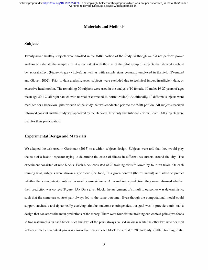
We adapted the task used in Gershman (2017) to a within-subjects design. Subjects were told that they would play
the role of a health inspector trying to determine the cause of illness in different restaurants around the city. The
experiment consisted of nine blocks. Each block consisted of 20 training trials followed by four test trials. On each
training trial, subjects were shown a given cue (the food) in a given context (the restaurant) and asked to predict
whether that cue-context combination would cause sickness. After making a prediction, they were informed whether
their prediction was correct (Figure 1A). On a given block, the assignment of stimuli to outcomes was deterministic,
such that the same cue-context pair always led to the same outcome. Even though the computational model could
support stochastic and dynamically evolving stimulus-outcome contingencies, our goal was to provide a minimalist
design that can assess the main predictions of the theory. There were four distinct training cue-context pairs (two foods
× two restaurants) on each block, such that two of the pairs always caused sickness while the other two never caused
sickness. Each cue-context pair was shown five times in each block for a total of 20 randomly shuffled training trials.
5
All rights reserved. No reuse allowed without permission. The copyright holder for this preprint (which was not peer-reviewed) is the author/funder.. https://doi.org/10.1101/228593doi: bioRxiv preprint
Cue/Choice(0-3 s = RT)
Feedback (1 s)
ITI (1-7 s + residual)
ISI (1 s)
Condition Trainingphase
Testphase
Irrelevant
x1c1+x2c1−x1c2+x2c2−
x1c1x1c3x3c1x3c3
Modulatory
x1c1+x2c1−x1c2−x2c2+
x1c1x1c3x3c1x3c3
Additive
x1c1+x2c1+x1c2−x2c2−
x1c1x1c3x3c1x3c3
A B
Figure 1. Experimental Design
(A) Timeline of events during a training trial. Subjects are shown a cue (food) and context (restaurant) and are asked
to predict whether the food will make a customer sick. They then see a line under the chosen option, and feedback
indicating a “Correct” or “Incorrect” response. ISI: interstimulus interval; ITI: intertrial interval.
(B) Stimulus-outcome contingencies in each condition. Cues denoted by (x1,x2,x3) and contexts denoted by
(c1,c2,c3). Outcome presentation denoted by “+” and no outcome denoted by “−”.
6
All rights reserved. No reuse allowed without permission. The copyright holder for this preprint (which was not peer-reviewed) is the author/funder.. https://doi.org/10.1101/228593doi: bioRxiv preprint
x r
c
x r
c
x r
c
cue outcome
context
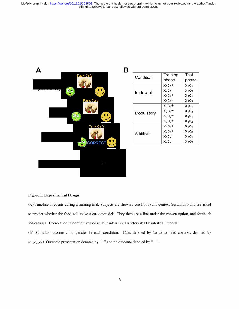
M1: irrelevant contextcue-outcome contingency is context-independent
M2: modulatory contextcue-outcome contingency is context-specific
M3: additive contextcontext acts like another cue
Figure 2. Hypothesis Space of Causal Structures
Each causal structure is depicted as a network where the nodes represent variables and the edges represent causal
connections. In M2, the context modulates the causal relationship between the cue and the outcome. Adapted from
Gershman (2017).
7
All rights reserved. No reuse allowed without permission. The copyright holder for this preprint (which was not peer-reviewed) is the author/funder.. https://doi.org/10.1101/228593doi: bioRxiv preprint
Crucially, the stimulus-outcome contingencies in each block were designed to promote a particular causal interpretation
of the environment (Figure 1B, Figure 2). On irrelevant context blocks, one cue caused sickness in both contexts,
while the other cue never caused sickness, thus rendering the contextual stimulus irrelevant for making correct
predictions. On modulatory context blocks, the cue-outcome contingency was reversed across contexts, such that
the same cue caused sickness in one context but not the other, and vice versa for the other cue. On these blocks,
context thus acted like an “occasion setter”, determining the sign of the cue-outcome association. Finally, on additive
context blocks, both cues caused sickness in one context but neither cue caused sickness in the other context, thus
favoring an interpretation of context acting as a punctate cue which sums together with other cues to determine the
outcome. There were no explicit instructions or other signals that indicated the different block conditions other than
the stimulus-outcome contingencies. While other interpretations of these contingencies are also possible (e.g., that
additive context sequences also match a causal structure in which cues are irrelevant), we sought to construct the
simplest stimulus-outcome relationships that distinguish between the three causal structures outlined in the Introduction.
These causal structures correspond to alternative hypotheses about the role of context in associative learning that have
been put forward in the animal learning literature (Balsam and Tomie, 1985). We based our experimental design on
the fact that a parsimonious model with these structures alone can capture a wide array of behavioral phenomena
(Gershman, 2017) and that the chosen stimuli-outcome contingencies establish a clear behavioral pattern that we can
build upon to explore the neural correlates of structure learning. The inherent asymmetry between cues and contexts is
justified by the a priori notion that foods (cues) are spatially and temporally confined focal stimuli, while restaurants
(contexts) often comprise spatially and temporally diffuse bundles of background stimuli.
Behavior was evaluated on four test trials during which subjects were similarly asked to make predictions, however
this time without receiving feedback. Subjects were presented with one novel cue and one novel context, resulting in
four (old cue vs. new cue) × (old context vs. new context) randomly shuffled test combinations (Figure 1B). The old
cue and the old context were always chosen such that their combination caused sickness during training. Importantly,
different causal structures predict different patterns of generalization on the remaining three trials which contain a new
cue and/or a new context. If context is deemed to be irrelevant, the old cue should always predict sickness, even when
8
All rights reserved. No reuse allowed without permission. The copyright holder for this preprint (which was not peer-reviewed) is the author/funder.. https://doi.org/10.1101/228593doi: bioRxiv preprint
presented in a new context. If a modulatory role of context is preferred, then no inferences can be made about any of
the three pairs that include a new cue or a new context. Finally, if context is interpreted as acting like another cue, then
both the old cue and the new cue should predict sickness in the old context but not in the new context.
Each block was assigned to one of the three conditions (irrelevant, modulatory, or additive) and each condition
appeared three times for each subject, for a total of nine blocks. The block order was randomized in groups of
three, such that the first three blocks covered all three conditions in a random order, and so did the next three blocks
and the final three blocks. We used nine sets of foods and restaurants corresponding to different cuisines (Chinese,
Japanese, Indian, Mexican, Greek, French, Italian, fast food and brunch). Each set consisted of three clipart food
images (cues) and three restaurant names (contexts). For each subject, blocks were randomly matched with cuisines,
such that subjects had to learn and generalize for a new set of stimuli on each block. The assignment of cuisines was
independent of the block condition. The valence of the stimuli was also randomized across subjects, such that the
same cue-context pair could predict sickness for some subjects but not others.
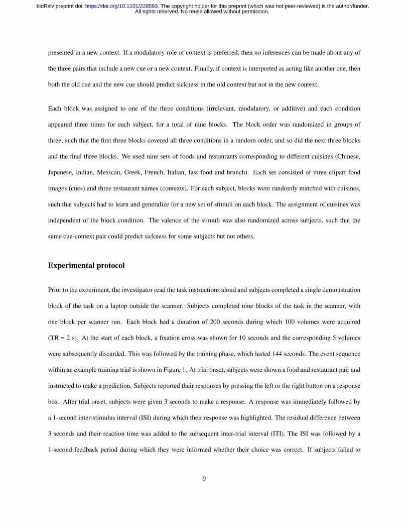
Experimental protocol
Prior to the experiment, the investigator read the task instructions aloud and subjects completed a single demonstration
block of the task on a laptop outside the scanner. Subjects completed nine blocks of the task in the scanner, with
one block per scanner run. Each block had a duration of 200 seconds during which 100 volumes were acquired
(TR = 2 s). At the start of each block, a fixation cross was shown for 10 seconds and the corresponding 5 volumes
were subsequently discarded. This was followed by the training phase, which lasted 144 seconds. The event sequence
within an example training trial is shown in Figure 1. At trial onset, subjects were shown a food and restaurant pair and
instructed to make a prediction. Subjects reported their responses by pressing the left or the right button on a response
box. After trial onset, subjects were given 3 seconds to make a response. A response was immediately followed by
a 1-second inter-stimulus interval (ISI) during which their response was highlighted. The residual difference between
3 seconds and their reaction time was added to the subsequent inter-trial interval (ITI). The ISI was followed by a
1-second feedback period during which they were informed whether their choice was correct. If subjects failed to
9
All rights reserved. No reuse allowed without permission. The copyright holder for this preprint (which was not peer-reviewed) is the author/funder.. https://doi.org/10.1101/228593doi: bioRxiv preprint
respond within 3 seconds of trial onset, no response was recorded and at feedback they were informed that they had
timed out. During the ITIs, a fixation cross was shown. The trial order and the jittered ITIs for the training phase were
generated using the optseq2 program (Greve, 2002) with ITIs between 1 and 12 seconds. The training phase was
followed by a 4 second message informing the subjects they are about to enter the test phase. The test phase lasted
36 seconds. Test trials had a similar structure as training trials, with the difference that subjects were given 6 seconds
to respond instead of 3 and there was no ISI nor feedback period. The ITIs after the first 3 test trials were 2, 4, and 6
seconds, randomly shuffled. The last training trial was followed by a 6-second fixation cross. The stimulus sequences
and ITIs were pre-generated for all subjects. The task was implemented using the PsychoPy2 package (Peirce, 2007).
The subjects in the behavioral pilot version of the study performed an identical version of the experiment, except that
it was conducted on a laptop.
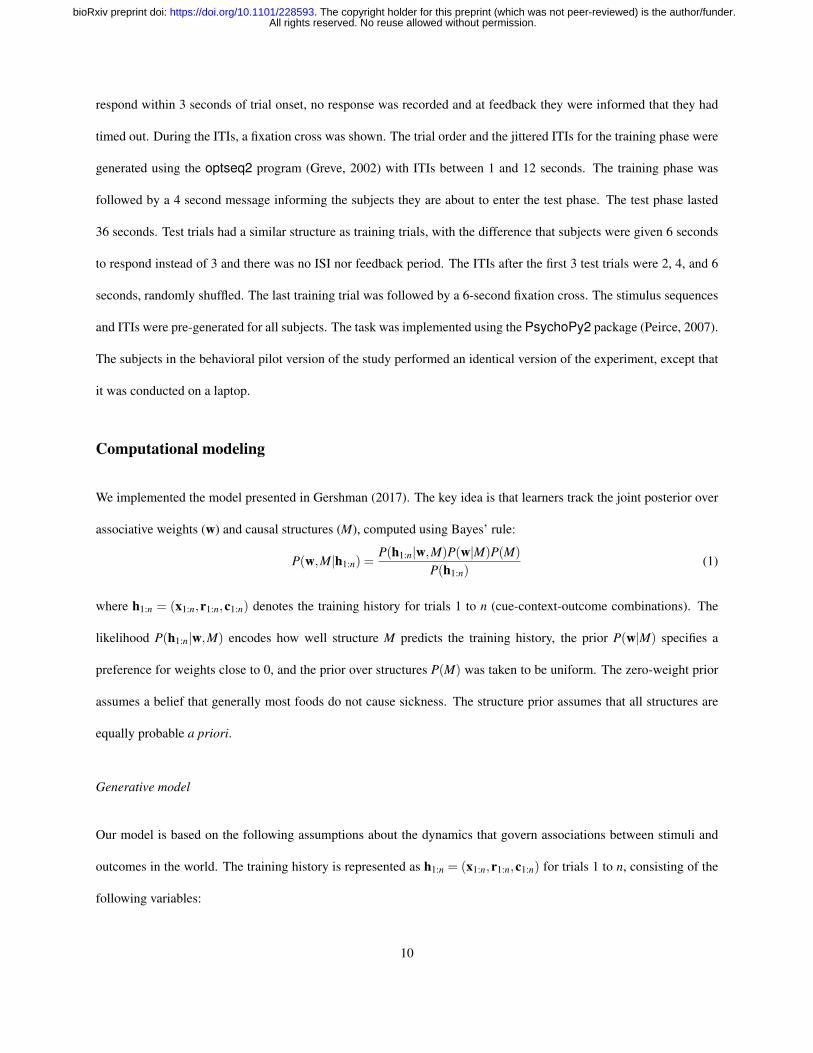
Computational modeling
We implemented the model presented in Gershman (2017). The key idea is that learners track the joint posterior over
associative weights (w) and causal structures (M), computed using Bayes’ rule:
P(w,M|h1:n) =P(h1:n|w,M)P(w|M)P(M)
P(h1:n)(1)
where h1:n = (x1:n,r1:n,c1:n) denotes the training history for trials 1 to n (cue-context-outcome combinations). The
likelihood P(h1:n|w,M) encodes how well structure M predicts the training history, the prior P(w|M) specifies a
preference for weights close to 0, and the prior over structures P(M) was taken to be uniform. The zero-weight prior
assumes a belief that generally most foods do not cause sickness. The structure prior assumes that all structures are
equally probable a priori.
Generative model
Our model is based on the following assumptions about the dynamics that govern associations between stimuli and
outcomes in the world. The training history is represented as h1:n = (x1:n,r1:n,c1:n) for trials 1 to n, consisting of the
following variables:
10
All rights reserved. No reuse allowed without permission. The copyright holder for this preprint (which was not peer-reviewed) is the author/funder.. https://doi.org/10.1101/228593doi: bioRxiv preprint
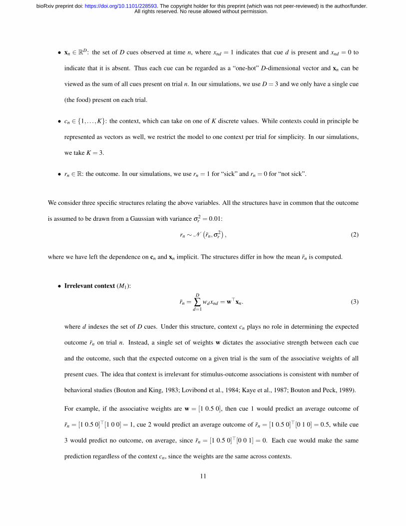
• xn ∈ RD: the set of D cues observed at time n, where xnd = 1 indicates that cue d is present and xnd = 0 to
indicate that it is absent. Thus each cue can be regarded as a “one-hot” D-dimensional vector and xn can be
viewed as the sum of all cues present on trial n. In our simulations, we use D = 3 and we only have a single cue
(the food) present on each trial.
• cn ∈ {1, . . . ,K}: the context, which can take on one of K discrete values. While contexts could in principle be
represented as vectors as well, we restrict the model to one context per trial for simplicity. In our simulations,
we take K = 3.
• rn ∈ R: the outcome. In our simulations, we use rn = 1 for “sick” and rn = 0 for “not sick”.
We consider three specific structures relating the above variables. All the structures have in common that the outcome
is assumed to be drawn from a Gaussian with variance σ2r = 0.01:
rn ∼N(rn,σ
2r), (2)
where we have left the dependence on cn and xn implicit. The structures differ in how the mean rn is computed.
• Irrelevant context (M1):
rn =D
∑d=1
wdxnd = w>xn. (3)
where d indexes the set of D cues. Under this structure, context cn plays no role in determining the expected
outcome rn on trial n. Instead, a single set of weights w dictates the associative strength between each cue
and the outcome, such that the expected outcome on a given trial is the sum of the associative weights of all
present cues. The idea that context is irrelevant for stimulus-outcome associations is consistent with number of
behavioral studies (Bouton and King, 1983; Lovibond et al., 1984; Kaye et al., 1987; Bouton and Peck, 1989).
For example, if the associative weights are w = [1 0.5 0], then cue 1 would predict an average outcome of
rn = [1 0.5 0]>[1 0 0] = 1, cue 2 would predict an average outcome of rn = [1 0.5 0]>[0 1 0] = 0.5, while cue
3 would predict no outcome, on average, since rn = [1 0.5 0]>[0 0 1] = 0. Each cue would make the same
prediction regardless of the context cn, since the weights are the same across contexts.
11
All rights reserved. No reuse allowed without permission. The copyright holder for this preprint (which was not peer-reviewed) is the author/funder.. https://doi.org/10.1101/228593doi: bioRxiv preprint
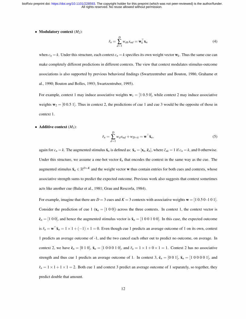
• Modulatory context (M2):
rn =D
∑d=1
wdkxnd = w>k xn (4)
when cn = k. Under this structure, each context cn = k specifies its own weight vector wk. Thus the same cue can
make completely different predictions in different contexts. The view that context modulates stimulus-outcome
associations is also supported by previous behavioral findings (Swartzentruber and Bouton, 1986; Grahame et
al., 1990; Bouton and Bolles, 1993; Swartzentruber, 1995).
For example, context 1 may induce associative weights w1 = [1 0.5 0], while context 2 may induce associative
weights w2 = [0 0.5 1]. Thus in context 2, the predictions of cue 1 and cue 3 would be the opposite of those in
context 1.
• Additive context (M3):
rn =D
∑d=1
wdxnd +wD+k = w>xn, (5)
again for cn = k. The augmented stimulus xn is defined as: xn = [xn, cn], where cnk = 1 if cn = k, and 0 otherwise.
Under this structure, we assume a one-hot vector cn that encodes the context in the same way as the cue. The
augmented stimulus xn ∈ RD+K and the weight vector w thus contain entries for both cues and contexts, whose
associative strength sums to predict the expected outcome. Previous work also suggests that context sometimes
acts like another cue (Balaz et al., 1981; Grau and Rescorla, 1984).
For example, imagine that there are D = 3 cues and K = 3 contexts with associative weights w = [1 0.5 0 -1 0 1].
Consider the prediction of cue 1 (xn = [1 0 0]) across the three contexts. In context 1, the context vector is
cn = [1 0 0], and hence the augmented stimulus vector is xn = [1 0 0 1 0 0]. In this case, the expected outcome
is rn = w>xn = 1×1+(−1)×1 = 0. Even though cue 1 predicts an average outcome of 1 on its own, context
1 predicts an average outcome of -1, and the two cancel each other out to predict no outcome, on average. In
context 2, we have cn = [0 1 0], xn = [1 0 0 0 1 0], and rn = 1× 1+ 0× 1 = 1. Context 2 has no associative
strength and thus cue 1 predicts an average outcome of 1. In context 3, cn = [0 0 1], xn = [1 0 0 0 0 1], and
rn = 1×1+1×1 = 2. Both cue 1 and context 3 predict an average outcome of 1 separately, so together, they
predict double that amount.
12
All rights reserved. No reuse allowed without permission. The copyright holder for this preprint (which was not peer-reviewed) is the author/funder.. https://doi.org/10.1101/228593doi: bioRxiv preprint
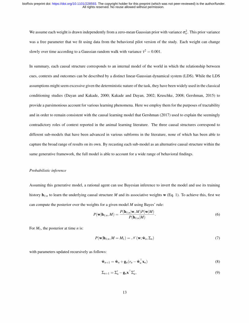
We assume each weight is drawn independently from a zero-mean Gaussian prior with variance σ2w. This prior variance
was a free parameter that we fit using data from the behavioral pilot version of the study. Each weight can change
slowly over time according to a Gaussian random walk with variance τ2 = 0.001.
In summary, each causal structure corresponds to an internal model of the world in which the relationship between
cues, contexts and outcomes can be described by a distinct linear-Gaussian dynamical system (LDS). While the LDS
assumptions might seem excessive given the deterministic nature of the task, they have been widely used in the classical
conditioning studies (Dayan and Kakade, 2000; Kakade and Dayan, 2002; Kruschke, 2008; Gershman, 2015) to
provide a parsimonious account for various learning phenomena. Here we employ them for the purposes of tractability
and in order to remain consistent with the causal learning model that Gershman (2017) used to explain the seemingly
contradictory roles of context reported in the animal learning literature. The three causal structures correspond to
different sub-models that have been advanced in various subforms in the literature, none of which has been able to
capture the broad range of results on its own. By recasting each sub-model as an alternative causal structure within the
same generative framework, the full model is able to account for a wide range of behavioral findings.
Probabilistic inference
Assuming this generative model, a rational agent can use Bayesian inference to invert the model and use its training
history h1:n to learn the underlying causal structure M and its associative weights w (Eq. 1). To achieve this, first we
can compute the posterior over the weights for a given model M using Bayes’ rule:
P(w|h1:n,M) =P(h1:n|w,M)P(w|M)
P(h1:n|M). (6)
For M1, the posterior at time n is:
P(w|h1:n,M = M1) = N (w; wn,Σn) (7)
with parameters updated recursively as follows:
wn+1 = wn +gn(rn− w>n xn) (8)
Σn+1 = Σ′n−gnx>Σ
′n, (9)
13
All rights reserved. No reuse allowed without permission. The copyright holder for this preprint (which was not peer-reviewed) is the author/funder.. https://doi.org/10.1101/228593doi: bioRxiv preprint
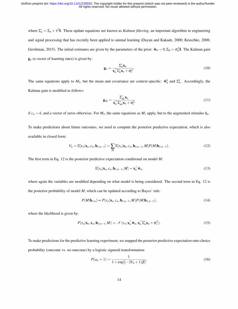
where Σ′n = Σn + τ2I. These update equations are known as Kalman filtering, an important algorithm in engineering
and signal processing that has recently been applied to animal learning (Dayan and Kakade, 2000; Kruschke, 2008;
Gershman, 2015). The initial estimates are given by the parameters of the prior: w0 = 0,Σ0 = σ2wI. The Kalman gain
gn (a vector of learning rates) is given by:
gn =Σ′nxn
x>n Σ′nxn +σ2r. (10)
The same equations apply to M2, but the mean and covariance are context-specific: wkn and Σk
n. Accordingly, the
Kalman gain is modified as follows:
gnk =Σ′nkxn
x>n Σ′nkxn +σ2r
(11)
if cn = k, and a vector of zeros otherwise. For M3, the same equations as M1 apply, but to the augmented stimulus xn.
To make predictions about future outcomes, we need to compute the posterior predictive expectation, which is also
available in closed form:
Vn = E[rn|xn,cn,h1:n−1] = ∑ME[rn|xn,cn,h1:n−1,M]P(M|h1:n−1). (12)
The first term in Eq. 12 is the posterior predictive expectation conditional on model M:
E[rn|xn,cn,h1:n−1,M] = x>n wn, (13)
where again the variables are modified depending on what model is being considered. The second term in Eq. 12 is
the posterior probability of model M, which can be updated according to Bayes’ rule:
P(M|h1:n) ∝ P(rn|xn,cn,h1:n−1,M)P(M|h1:n−1), (14)
where the likelihood is given by:
P(rn|xn,cn,h1:n−1,M) = N (rn;x>n wn,x>n Σ′nxn +σ
2r ). (15)
To make predictions for the predictive learning experiment, we mapped the posterior predictive expectation onto choice
probability (outcome vs. no outcome) by a logistic sigmoid transformation:
P(an = 1) =1
1+ exp[(−2Vn +1)β ], (16)
14
All rights reserved. No reuse allowed without permission. The copyright holder for this preprint (which was not peer-reviewed) is the author/funder.. https://doi.org/10.1101/228593doi: bioRxiv preprint

where an = 1 indicates a prediction that the outcome will occur, and an = 0 indicates a prediction that the outcome
will not occur. The free parameter β corresponds to the inverse softmax temperature and was fit based on data from
the behavioral pilot portion of the study.
In summary, we use standard Kalman filtering to infer the parameters of the LDS corresponding to each causal
structure. This yields a distribution over associative weights w for each causal structure M (Eq. 6), which we can
use in turn to compute a distribution over all three causal structures (Eq. 14). The joint distribution over weights and
causal structures is then used to predict the expected outcome Vn (Eq. 12) and the corresponding decision an (Eq. 16).
Our model thus makes predictions about computations at two levels of inference: at the level of causal structures
(Eq. 14) and at the level of associative weights for each structure (Eq. 6).
Parameter estimation
The model has two free parameters: the variance σ2w of the Gaussian prior from which the weights are assumed to
be drawn, and the inverse temperature β used in the logistic transformation from predictive posterior expectation to
choice probability. Intuitively, the former corresponds to the level of uncertainty in the initial estimate of the weights,
while the latter reflects choice stochasticity. We estimated a single set of parameters based on choice data from the
behavioral pilot version of the study using maximum log-likelihood estimation (Figure 4B, grey circles). We preferred
this approach over estimating a separate set of parameters for each subject as it tends to avoid overfitting, produces
more stable estimates, and has been frequently used in previous studies (Daw et al., 2006; Gershman et al., 2009;
Gläscher, 2009; Gläscher et al., 2010). Additionally, since none of these pilot subjects participated in the fMRI portion
of the study, this procedure ensured that the parameters used in the final analysis were not overfit to the choices of the
scanned subjects. For the purposes of fitting, the model was trained and tested over the same stimulus sequences as
the pilot subjects. Each block was simulated independently i.e. the parameters of the model were reset to their initial
values prior to the start of training. The likelihood of the subject’s response on a given trial was estimated according
to the choice probability given by the model on that trial. Maximum log-likelihood estimation was computed using
MATLAB’s fmincon function with 5 random initializations. The bounds on the parameters were σ2w ∈ [0,1] and
15
All rights reserved. No reuse allowed without permission. The copyright holder for this preprint (which was not peer-reviewed) is the author/funder.. https://doi.org/10.1101/228593doi: bioRxiv preprint
β ∈ [0,10].
The fitted values were σ2w = 0.12 and β = 2.01. All other parameters were set to the same values as described in
Gershman (2017). We used these parameters to simulate subjects from the fMRI experiment. For behavioral analysis,
we trained and tested the model on each block separately and reported the choice probabilities on test trials, averaged
across conditions. We used the probability distributions from these simulations to compute the parametric modulators
(the Kullback-Leibler divergence) in the GLM (Figure 5) and the representational dissimilarity matrices (Figure 6).
For model comparison, we similarly estimated parameters for versions of model constrained to use a single causal
structure (M1, M2, or M3). We used random effects Bayesian model selection (Rigoux et al., 2014) to compare the three
single-structure models and the full model, using -0.5 * BIC as an approximation of the log model evidence, where
BIC is the Bayesian information criterion. Models were compared based on their computed exceedance probabilities,
with a higher exceedance probability indicating a higher frequency of the given model in the population compared to
the other models.
fMRI data acquisition
Scanning was carried out on a 3T Siemens Magnetom Prisma MRI scanner with the vendor 32-channel head coil
(Siemens Healthcare, Erlangen, Germany) at the Harvard University Center for Brain Science Neuroimaging. A
T1-weighted
high-resolution multi-echo magnetization-prepared rapid-acquisition gradient echo (ME-MPRAGE) anatomical scan
(van der Kouwe et al., 2008) of the whole brain was acquired for each subject prior to any functional scanning (176
saggital slices, voxel size = 1.0 x 1.0 x 1.0 mm, TR = 2530 ms, TE = 1.69 - 7.27 ms, TI = 1100 ms, flip angle = 7◦, FOV
= 256 mm). Functional images were acquired using a T2*-weighted echo-planar imaging (EPI) pulse sequence that
employed multiband RF pulses and Simultaneous Multi-Slice (SMS) acquisition (Moeller et al., 2010; Feinberg et al.,
2010; Xu et al., 2013). In total, 9 functional runs were collected per subject, with each run corresponding to a single
task block (84 interleaved axial-oblique slices per whole brain volume, voxel size = 1.5 x 1.5 x 1.5 mm, TR = 2000
16
All rights reserved. No reuse allowed without permission. The copyright holder for this preprint (which was not peer-reviewed) is the author/funder.. https://doi.org/10.1101/228593doi: bioRxiv preprint
ms, TE = 30 ms, flip angle = 80◦, in-plane acceleration (GRAPPA) factor = 2, multi-band acceleration factor = 3, FOV
= 204 mm). The initial 5 TRs (10 seconds) were discarded as the scanner stabilized. Functional slices were oriented
to a 25 degree tilt towards coronal from AC-PC alignment. The SMS-EPI acquisitions used the CMRR-MB pulse
sequence from the University of Minnesota. Four subjects failed to complete all 9 functional runs due to technical
reasons and were excluded from the analyses. Three additional subjects were excluded due to excessive motion.
fMRI preprocessing
Functional images were preprocessed and analyzed using SPM12 (Wellcome Department of Imaging Neuroscience,
London, UK). Each functional scan was realigned to correct for small movements between scans, producing an
aligned set of images and a mean image for each subject. The high-resolution T1-weighted ME-MPRAGE images
were then co-registered to the mean realigned images and the gray matter was segmented out and normalized to the
gray matter of a standard Montreal Neurological Institute (MNI) reference brain. The functional images were then
normalized to the MNI template (resampled voxel size 2 mm isotropic), spatially smoothed with a 8 mm full-width at
half-maximum (FWHM) Gaussian kernel, high-pass filtered at 1/128 Hz, and corrected for temporal autocorrelations
using a first-order autoregressive model.
Univariate analysis
To analyze the fMRI data, we defined a GLM with four impulse regressors convolved with the canonical hemodynamic
response function (HRF): a regressor at trial onset for all training trials (the stimulus regressor); a regressor at feedback
onset for all training trials (the feedback regressor); a regressor at feedback onset for training trials on which the
subject produced the wrong response (the error regressor); and a regressor at feedback onset for training trials on
which the contextual stimulus differs from the contextual stimulus on the previous trial (the context regressor). The
context regressor was not included on the first training trial of each block. The feedback regressor had two parametric
modulators: the Kullback-Leibler (KL) divergence between the posterior and the prior probability distribution over
causal structures; and the KL divergence between the posterior and the prior probability distribution over the associative
weights for the causal structure corresponding to the condition of the given block. In particular, the causal structure
17
All rights reserved. No reuse allowed without permission. The copyright holder for this preprint (which was not peer-reviewed) is the author/funder.. https://doi.org/10.1101/228593doi: bioRxiv preprint
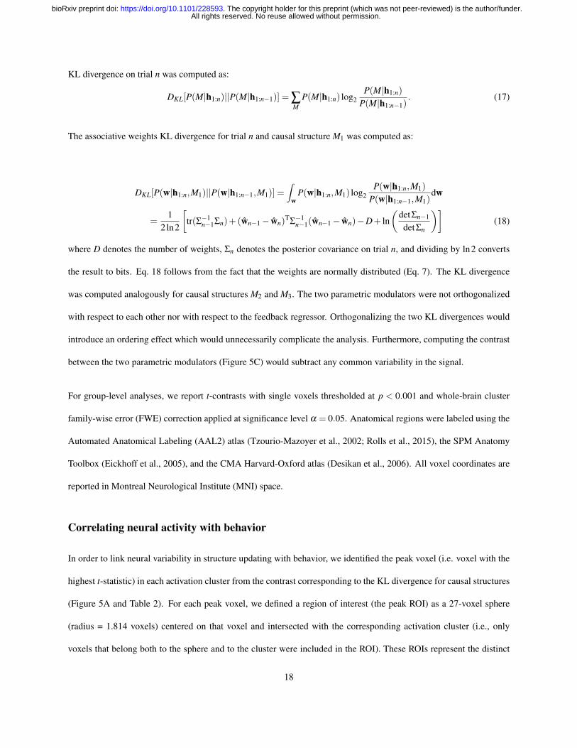
KL divergence on trial n was computed as:
DKL[P(M|h1:n)||P(M|h1:n−1)] = ∑M
P(M|h1:n) log2P(M|h1:n)
P(M|h1:n−1). (17)
The associative weights KL divergence for trial n and causal structure M1 was computed as:
DKL[P(w|h1:n,M1)||P(w|h1:n−1,M1)] =∫
wP(w|h1:n,M1) log2
P(w|h1:n,M1)
P(w|h1:n−1,M1)dw
=1
2ln2
[tr(Σ−1
n−1Σn)+(wn−1− wn)T
Σ−1n−1(wn−1− wn)−D+ ln
(detΣn−1
detΣn
)](18)
where D denotes the number of weights, Σn denotes the posterior covariance on trial n, and dividing by ln2 converts
the result to bits. Eq. 18 follows from the fact that the weights are normally distributed (Eq. 7). The KL divergence
was computed analogously for causal structures M2 and M3. The two parametric modulators were not orthogonalized
with respect to each other nor with respect to the feedback regressor. Orthogonalizing the two KL divergences would
introduce an ordering effect which would unnecessarily complicate the analysis. Furthermore, computing the contrast
between the two parametric modulators (Figure 5C) would subtract any common variability in the signal.
For group-level analyses, we report t-contrasts with single voxels thresholded at p < 0.001 and whole-brain cluster
family-wise error (FWE) correction applied at significance level α = 0.05. Anatomical regions were labeled using the
Automated Anatomical Labeling (AAL2) atlas (Tzourio-Mazoyer et al., 2002; Rolls et al., 2015), the SPM Anatomy
Toolbox (Eickhoff et al., 2005), and the CMA Harvard-Oxford atlas (Desikan et al., 2006). All voxel coordinates are
reported in Montreal Neurological Institute (MNI) space.
Correlating neural activity with behavior
In order to link neural variability in structure updating with behavior, we identified the peak voxel (i.e. voxel with the
highest t-statistic) in each activation cluster from the contrast corresponding to the KL divergence for causal structures
(Figure 5A and Table 2). For each peak voxel, we defined a region of interest (the peak ROI) as a 27-voxel sphere
(radius = 1.814 voxels) centered on that voxel and intersected with the corresponding activation cluster (i.e., only
voxels that belong both to the sphere and to the cluster were included in the ROI). These ROIs represent the distinct
18
All rights reserved. No reuse allowed without permission. The copyright holder for this preprint (which was not peer-reviewed) is the author/funder.. https://doi.org/10.1101/228593doi: bioRxiv preprint
brain areas that are most strongly correlated with causal structure updating. For each block and for each subject, we
then extracted the structure KL betas of the voxels in each ROI. Since the betas are computed for each block separately
as an intermediate step in fitting the GLM, we did not have to perform any additional analyses in order to obtain them.
For a given block, the structure KL beta of a particular voxel represents the degree to which BOLD activity in that
voxel tracks the causal structure KL divergence across all 20 training trials of the block. Even for voxels that are on
average highly correlated with the KL divergence (such as the peak voxels), there is block-to-block variability in the
strength of that relationship. If the activity of a given voxel represents updates about causal structures, a lower beta on
a particular block would suggest that the underlying computations deviated from Bayesian updating as predicted by
the model. Conversely, a high beta would indicate that the computations were consistent with the structure learning
account. Thus one would expect that performance on the test phase following a given block would be similar to the
predictions of the Bayesian model in the latter case but not in the former. We tested this idea by correlating the average
beta across all voxels in the peak ROI for a given training block with the average log likelihood of the subject’s choices
on the test trials following that block. This yielded a Pearson’s correlation coefficient (n = 9 blocks per subject) for
each subject. The resulting correlation coefficients were Fisher z-transformed and entered into a one-sample t-test
against 0. For each peak ROI, we report the average Fisher z-transformed r and the result from the t-test (Figure 5D).
Primary sensory, visual, and motor regions such as V1 and the cerebellum were a priori excluded from this analysis.
Negative activation clusters were also excluded. We chose spherical ROIs of this size in order to remain consistent
with our searchlight analysis and with previous studies (Chan et al., 2016). Similarity between the model predictions
and the subject’s behavior was computed as the mean log likelihood of their choices across test trials on which they
produced a response, 〈logP(cn)〉, where cn = 1 indicates that the subject predicted the outcome would occur on trial n,
cn = 0 indicates that they predicted the outcome would not occur, and the probability P(cn) is calculated as in Eq. 16.
Representational similarity analysis
We used representational similarity analysis (RSA) to identify candidate brain regions that might encode the full
probability distribution over causal structures in their multivariate activity patterns (Kriegeskorte et al., 2008; Xue et
19
All rights reserved. No reuse allowed without permission. The copyright holder for this preprint (which was not peer-reviewed) is the author/funder.. https://doi.org/10.1101/228593doi: bioRxiv preprint

al., 2010; Chan et al., 2016). On a given trial, we expected Bayesian updating to occur when the outcome of the
subject’s prediction is presented at feedback onset (i.e. whether they were correct or incorrect). We therefore expected
to find representations of the prior distribution at trial onset and representations of the posterior distribution at feedback
onset (which in turn corresponds to the prior distribution on the following trial). We describe how we performed RSA
for the prior; the analysis for the posterior proceeded in a similar fashion.
In order to identify regions with a high representational similarity match for the prior, we used an unbiased whole-brain
“searchlight” approach. For each voxel of the entire volume, we defined a 27-voxel spherical ROI (radius = 1.814
voxels) centered on that voxel, excluding voxels outside the brain. For each subject and each ROI, we computed a
180× 180 representational dissimilarity matrix R (the neural RDM) such that the entry in row i and column j is the
cosine distance between the neural activity patterns on training trial i and training trial j:
Ri j = R ji = 1− cosθi j = 1−ai ·a j
|ai| |a j|(19)
where θi j is the angle between the 27-dimensional vectors ai and a j which represent the instantaneous neural activity
patterns at trial onset on training trials i and j, respectively, in the given ROI for the given subject. Neural activations
entered into the RSA were obtained using a GLM with distinct impulse regressors convolved with the HRF at trial
onset and feedback onset on each trial (test trials had regressors at trial onset only). The neural activity of a given
voxel was thus simply its beta coefficient of the regressor for the corresponding trial and event. Since the matrix is
symmetric and Rii = 0, we only considered entries above the diagonal (i.e. i < j). The cosine distance is equal to 1
minus the normalized correlation (i.e. the cosine of the angle between the two vectors), which has been preferred over
other similarity measures as it better conforms to intuitions about similarity both for neural activity and for probability
distributions (Chan et al., 2016).
Similarly, we computed an RDM (the model RDM) such that the entry in row i and column j is the cosine distance
between the priors on training trial i and training trial j, as computed by model simulations using the stimulus
sequences experienced by the subject on the corresponding blocks.
20
All rights reserved. No reuse allowed without permission. The copyright holder for this preprint (which was not peer-reviewed) is the author/funder.. https://doi.org/10.1101/228593doi: bioRxiv preprint
If neural activity in the given ROI encodes the prior, then the neural RDM should resemble the model RDM: trials
on which the prior is similar should have similar neural representations (i.e. smaller cosine distances), while trials
on which the prior is dissimilar should have dissimilar neural representations (i.e. larger cosine distances). This
intuition can be formalized using Spearman’s rank correlation coefficient between the model RDM and the neural
RDM (n= 180×179/2= 16110 unique pairs of trials in each RDM). A high coefficient implies that pairs of trials with
similar priors tend show similar neural patterns while pairs of trials with dissimilar priors tend to show dissimilar neural
patterns. Spearman’s rank correlation is a preferred method for comparing RDMs over other correlation measures as
it does not assume a linear relationship between the RDMs (Kriegeskorte et al., 2008). Thus for each voxel and each
subject, we obtained a single Spearman’s ρ that reflects the representational similarity match between the prior and
the ROI around that voxel.
In order to aggregate these results across subjects, for each voxel we Fisher z-transformed the resulting Spearman’s ρ
from all 20 subjects and performed a t-test against 0. This yielded a group-level t-map, where the t-value of each voxel
indicates whether the representational similarity match for that voxel is significant across subjects. We thresholded
single voxels at p < 0.001 and corrected for multiple comparisons using whole-brain cluster FWE correction at
significance level α = 0.05. We report the surviving clusters and the t-values of the corresponding voxels (Figure 6A).
We used an identical procedure to obtain a t-map indicating which brain regions how a high representational similarity
match with the posterior (Figure 6B). The only difference was that we computed the neural RDMs using activity
patterns at feedback onset (rather than at trial onset) and we computed the model RDMs using the posterior (instead
of the prior).
Finally, since both the prior and the posterior tend to be similar on trials that are temporally close to each other, as well
as on trials from the same block, we computed two control RDMs: a “time RDM” in which the distance between trials
i and j is |ti− t j|, where ti is the difference between the onset of trial i and the start of its corresponding block; and a
“block RDM” in which the distance between trials i and j is 0 if they belong to the same block, and 1 otherwise. Each
Spearman’s ρ’s was then computed as a partial rank correlation coefficient between the neural RDM and the model
21
All rights reserved. No reuse allowed without permission. The copyright holder for this preprint (which was not peer-reviewed) is the author/funder.. https://doi.org/10.1101/228593doi: bioRxiv preprint

0 5 10 15 20trial #
0.4
0.5
0.6
0.7
0.8
0.9
1ac
cura
cyBehavioral pilotA
modelsubjects
0 5 10 15 20trial #
0.4
0.5
0.6
0.7
0.8
0.9
1
accu
racy
fMRIB
modelsubjects
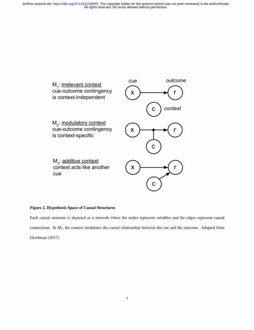
Figure 3. Learning curves during training
Performance during training for (A) behavioral pilot subjects (N = 10), and (B) fMRI subjects (N = 20), averaged
across subjects and blocks. The prior variance of the weights σ2w and the logistic inverse temperature β were fitted
using data only from the pilot version of the study.
RDM, controlling for the time RDM and the block RDM. This rules out the possibility that our RSA results reflect
within-block temporal autocorrelations that are unrelated to the prior or the posterior.
Results
Causal structure learning accounts for behavioral performance
The behavioral results replicated the findings of Gershman (2017) using a within-subject design. Subjects from both
the pilot and the fMRI portions of the study learned the correct stimulus-outcome associations relatively quickly, with
average performance plateauing around the middle of training (Figure 3). Average accuracy during the second half of
training was 91.2±2.5% (t9 = 16.8, p < 10−7, one-sample t-test against 50%) for the pilot subjects, and 92.7±1.7%
(t19 = 25.0, p < 10−15, one-sample t-test against 50%) for the scanned subjects, well above chance.
22
All rights reserved. No reuse allowed without permission. The copyright holder for this preprint (which was not peer-reviewed) is the author/funder.. https://doi.org/10.1101/228593doi: bioRxiv preprint
A
Irrelevant training Modulatory training Additive training0
0.2
0.4
0.6
0.8
1
Pos
terio
r pr
obab
ility
M1M2M3
B
Irrelevant training Modulatory training Additive training0
0.2
0.4
0.6
0.8
1
Cho
ice
prob
abili
ty
x1c1
x1c3
x3c1
x3c3
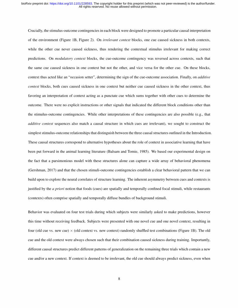
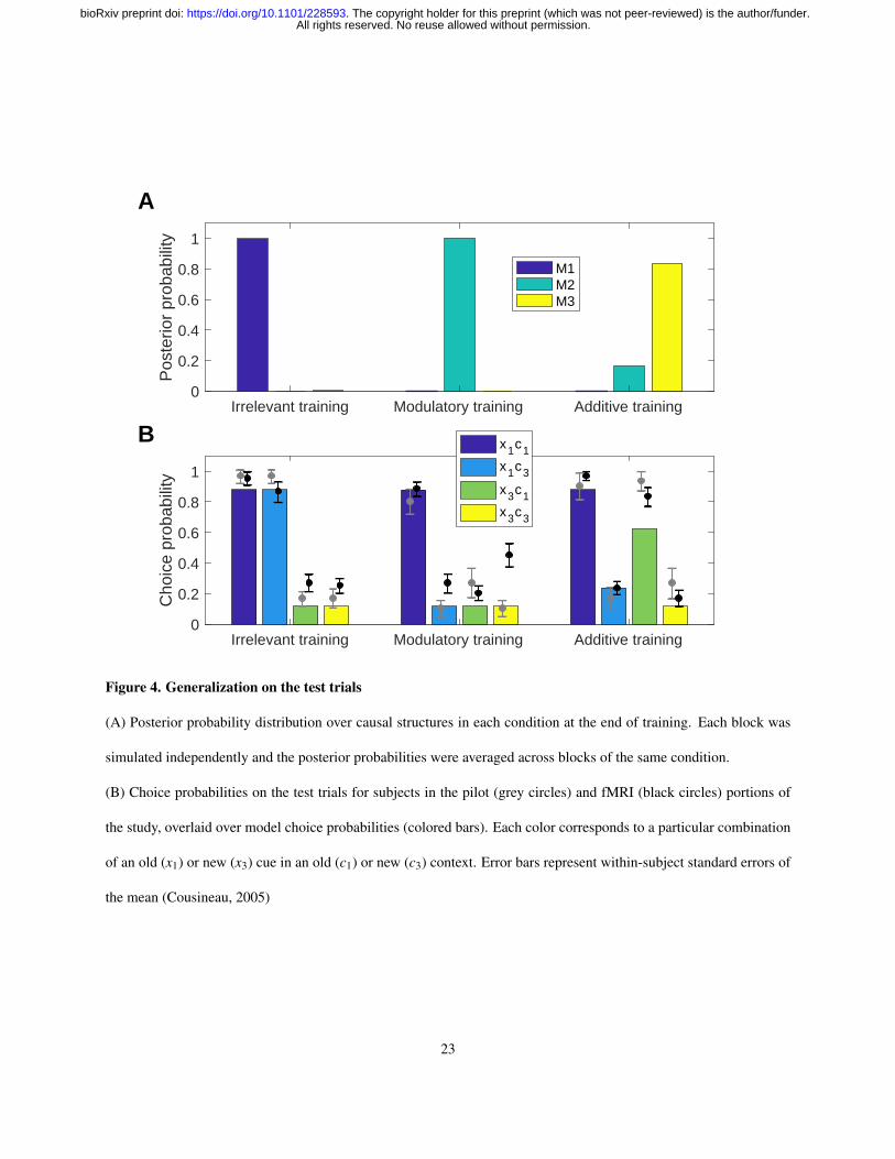
Figure 4. Generalization on the test trials
(A) Posterior probability distribution over causal structures in each condition at the end of training. Each block was
simulated independently and the posterior probabilities were averaged across blocks of the same condition.
(B) Choice probabilities on the test trials for subjects in the pilot (grey circles) and fMRI (black circles) portions of
the study, overlaid over model choice probabilities (colored bars). Each color corresponds to a particular combination
of an old (x1) or new (x3) cue in an old (c1) or new (c3) context. Error bars represent within-subject standard errors of
the mean (Cousineau, 2005)
23
All rights reserved. No reuse allowed without permission. The copyright holder for this preprint (which was not peer-reviewed) is the author/funder.. https://doi.org/10.1101/228593doi: bioRxiv preprint
Importantly, both groups exhibited distinct patterns of generalization on the test trials across the different conditions,
consistent with the results of Gershman (2017) (Figure 4B). Without taking the computational model into account,
these generalization patterns already suggest that subjects learned something beyond simple stimulus-response mappings.
On blocks during which context was irrelevant (Figure 4B, irrelevant training), subjects tended to predict that the old
cue x1, which caused sickness in both c1 and c2, would also cause sickness in the new context c3 (circle for x1c3),
even though they had never experienced c3 before. The new cue x3, on the other hand, was judged to be much less
predictive of sickness in either context (t38 = 9.51, p < 10−10, paired t-test). Conversely, on blocks during which
context acted like another cue (Figure 4B, additive training), subjects guessed that both cues would cause sickness in
the old context c1 (circle for x3c1), but not in the new context c3 (t38 = 11.1, p < 10−12, paired t-test). Generalization
in both of these conditions was different from what one would expect if subjects treated each cue-context pair as a
unique stimulus independent from the other pairs, which is similar to the generalization pattern on modulatory blocks
(Figure 4B, modulatory training). On these blocks, subjects judged that the old cue is predictive of sickness in the old
context significantly more compared to the remaining cue-context pairs (t38 = 9.01, p < 10−10, paired t-test).
These observations were consistent with the predictions of the computational model. Using parameters fit with data
from the behavioral pilot version of the study, the model quantitatively accounted for the generalization pattern on
the test trials choices of subjects in the fMRI portion of the study (Figure 4B; r = 0.96, p < 10−6). As expected, the
stimulus-outcome contingencies induced the model to infer a different causal structure in each of the three conditions
(Figure 4A), leading to the distinct response patterns on the simulated test trials. For comparison, we also ran versions
of the model using a single causal structure. Theories corresponding to each of these sub-models have been put forward
in the literature as explanations of the role of context during learning, however neither of them has been able to provide
a comprehensive account of the behavioral findings on its own. Accordingly, model performance was markedly worse
when the hypothesis space was restricted to a single causal structure: the correlation coefficients were r = 0.61 for the
irrelevant context structure (M1; p = 0.04), r = 0.73 for the modulatory context structure (M2; p < 0.01), and r = 0.91
for the additive context structure (M3; p < 0.0001). Bayesian model comparison confirmed the superiority of the full
structure learning model over the restricted variants (Table 1).
24
All rights reserved. No reuse allowed without permission. The copyright holder for this preprint (which was not peer-reviewed) is the author/funder.. https://doi.org/10.1101/228593doi: bioRxiv preprint

Hypotheses σ2w β BIC PXP Log lik Pearson’s r
M1,M2,M3 0.1249 2.0064 1670 0.3855 -1711 r = 0.96, p < 10−6
M1 0.0161 1.2323 2631 0.2048 -2687 r = 0.61, p = 0.036
M2 0.9997 1.7433 1828 0.2049 -1895 r = 0.73, p = 0.008
M3 0.0130 1.7508 2184 0.2048 -2180 r = 0.91, p = 0.00004
Table 1. Model comparison. Each model is represented by its corresponding hypothesis space of causal structures
(Figure 2). The free parameters σ2w and β were fit based on choice data from the pilot version of the study (Figure 4B,
grey circles). Log likelihood and Pearson’s r were computed based on choice data from the fMRI version of the study.
Bayesian information criterion (BIC) and protected exceedance probability (PXP) were computed on the pilot data.
Log lik, log likelihood.
Separate brain regions support structure learning and associative learning
We sought to identify brain regions in which the blood oxygenation level dependent (BOLD) signal tracks beliefs
about the underlying causal structure. In order to condense these multivariate distributions into scalars, we computed
the Kullback-Leibler (KL) divergence between the posterior and the prior distribution over causal structures on
each training trial, which measures the degree to which structural beliefs were revised after observing the outcome.
Specifically, we analyzed the fMRI data using a general linear model (GLM) which included the KL divergence as
a parametric modulator at feedback onset. We reasoned that activity in regions involved in learning causal structure
would correlate with the degree of belief revision.
A high KL divergence often implies that, before receiving feedback on the current trial, the agent had inferred the
wrong causal structure. Accordingly, we found that the KL divergence was relatively higher for trials on which subjects
produced an incorrect response (two-sample t-test, t3598 = 12.2, p < 10−30). To eliminate any confounds specifically
related to receiving negative feedback about incorrect responding, we included an error regressor at feedback onset
indicating trials on which subjects made an incorrect prediction. In addition, since the structures are sensitive to
25
All rights reserved. No reuse allowed without permission. The copyright holder for this preprint (which was not peer-reviewed) is the author/funder.. https://doi.org/10.1101/228593doi: bioRxiv preprint
Causal structure update Associative weights update
Causal structure update >associative weights update Structure updating predicts test choices
* **
IFG pars orbitalis (R)
Angular gyrus (R
)
IFG pars opercularis (R)
Frontal Pole (L
)
Angular gyrus (L
)
Middle orbital gyrus (R)
IFG pars opercularis (L)
Inferior temporal gyrus (R
)
Lingual gyrus (R)
-0.2
0
0.2
0.4
0.6F
ishe
r z-
tran
sfor
med
r
A B
C D
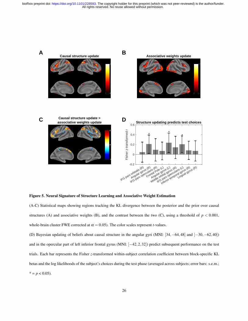
Figure 5. Neural Signature of Structure Learning and Associative Weight Estimation
(A-C) Statistical maps showing regions tracking the KL divergence between the posterior and the prior over causal
structures (A) and associative weights (B), and the contrast between the two (C), using a threshold of p < 0.001,
whole-brain cluster FWE corrected at α = 0.05). The color scales represent t-values.
(D) Bayesian updating of beliefs about causal structure in the angular gyri (MNI: [34,−64,48] and [−30,−62,40])
and in the opercular part of left inferior frontal gyrus (MNI: [−42,2,32]) predict subsequent performance on the test
trials. Each bar represents the Fisher z-transformed within-subject correlation coefficient between block-specific KL
betas and the log likelihoods of the subject’s choices during the test phase (averaged across subjects; error bars: s.e.m.;
* = p < 0.05).
26
All rights reserved. No reuse allowed without permission. The copyright holder for this preprint (which was not peer-reviewed) is the author/funder.. https://doi.org/10.1101/228593doi: bioRxiv preprint
contextual stimuli by design, the KL divergence tended to be higher when context changed from the previous trial
(two-sample t-test, t3418 = 6.53, p < 10−10). In order to account for potential effects of contextual tracking, we
thus included a regressor at feedback onset on trials on which the contextual stimulus differs from the previous
trial. Finally, since we were interested in regions that correlate with learning on the level of causal structures rather
than their associative weights, we included the KL divergence between the posterior and the prior distribution over
associative weights for the causal structure corresponding to the condition of the given block (e.g., only the weights
for the modulatory structure were analyzed on modulatory blocks). These weights encode the strength of causal
relationships between cues and outcomes (and additionally context, in the case of the additive structure). Including
this KL divergence as an additional parametric modulator at feedback onset would capture any variability in the signal
related to weight updating and allow us to isolate it from the signal related to structure updating.
We computed three group-level contrasts: the KL divergence for causal structures, the KL divergence for associative
weights, and the difference between the two. Activation clusters in all contrasts were identified by thresholding single
voxels at p < 0.001 and applying whole-brain cluster FWE correction at significance level α = 0.05. The first contrast
revealed several regions that were associated with updating of the posterior over causal structures (Figure 5A, and
Table 2). We observed bilateral parietal clusters with peak activations in the angular gyri. We also found bilateral
clusters in inferior frontal gyrus (IFG) spanning the opercular and the triangular parts of IFG. Bilateral activations
were also found in rostrolateral PFC, extending into the medial and anterior orbital gyri in the right hemisphere and
into the anterior insula and the orbital part of IFG in the left hemisphere. There was a cluster around the orbital
part of IFG in the right hemisphere as well. Significant activations were also found in bilateral cerebellum, bilateral
supplementary motor area (SMA), and in left inferior and middle temporal gyrus.
The second contrast revealed a more posterior network of brain regions that was correlated with the KL divergence
for associative weights (Figure 5B, and Table 3). We found a large cluster spanning visual cortex bilaterally and
extending into inferior parietal and inferior temporal cortex. We observed bilateral activations in IFG that were similar
to those observed in the causal structures KL contrast. There were also activations in the orbital part of bilateral IFG,
left middle temporal gyrus, and bilateral SMA. We also found subcortical activations in right thalamus and bilateral
27
All rights reserved. No reuse allowed without permission. The copyright holder for this preprint (which was not peer-reviewed) is the author/funder.. https://doi.org/10.1101/228593doi: bioRxiv preprint
ventral striatum.
In order to isolate regions that are specifically related to causal structure updating and not associative weight updating,
we computed the contrast between these two regressors (Figure 5C, and Table 4). Positive activations in this contrast
correspond to areas where the signal is more strongly correlated with the causal structures KL divergence than with
the associative weights KL divergence, while negative activations indicate the opposite relationship. This contrast
highlighted essentially the same areas as the single regressor contrast with the causal structures KL divergence
(Figure 5A, and Table 2), implying that the signal in these areas cannot be explained by associative learning alone
and suggesting a dissociable network of regions that might support structure learning. It is worth noting that the
regions which correlated more strongly with associative weight updating were in bilateral insula, bilateral precuneus,
and left supramarginal gyrus. Inspecting the single regressor contrasts revealed that these regions were either not
significantly correlated or were negatively correlated with both regressors. This suggests that their negative activation
here is due to a more negative correlation with the causal structures KL divergence, rather than to a positive correlation
with the associative weights KL divergence or a common representation of both types of updating.
Neural correlates of causal structure updating during training predict subsequent test performance
We hypothesized that if a neural signal correlates with updating beliefs about causal structure during training, it should
also be associated with variability in behavior during the test trials. For each block and for each subject, we computed
the average parameter estimate of the causal structure KL regressors across voxels in a 27-voxel spherical region of
interest (ROI) centered on the peak voxel from each activation cluster (i.e. the peak voxels from Table 2; see Materials
and Methods). Intuitively, these averaged betas (the KL betas) correspond to how strongly the voxels from a given
ROI correlate with the causal structure KL divergence during the training trials of a given block. If a particular region
mediates structure learning, then variability in its KL beta should predict variability in test phase behavior across
blocks. Accordingly, for each subject and each ROI, we correlated the KL beta across blocks with the log likelihood
of the subject’s responses on the test trials given the model predictions. The test log likelihood indicates how closely
the subject’s responses conform to the model predictions. For example, if on a particular block subjects are updating
28
All rights reserved. No reuse allowed without permission. The copyright holder for this preprint (which was not peer-reviewed) is the author/funder.. https://doi.org/10.1101/228593doi: bioRxiv preprint
Sign Brain region BA Extent t-value MNI coord.
Positive IFG pars orbitalis (R) 47 263 9.474 32 22 0
Angular gyrus (R) 39 1539 8.687 34 -64 48
IFG pars opercularis (R) 44 1411 7.483 48 20 32
Rostrolateral PFC (L) 10 1305 7.406 -40 56 6
Angular gyrus (L) 39 1500 7.343 -30 -62 40
Rostrolateral PFC (R) 10 789 7.296 36 54 0
IFG pars opercularis (L) 44 1560 6.999 -42 2 32
Supplementary motor area (L) 6 868 6.286 -6 8 52
Cerebelum (R) 660 6.217 18 -70 -24
Cerebelum (L) 1378 5.913 -6 -76 -28
Cerebelum (L) 207 5.646 -32 -68 -52
Inferior temporal gyrus (R) 20 159 5.533 62 -24 -22
Lingual gyrus (R) 19 225 5.364 12 -96 -8
Middle temporal gyrus (L) 21 187 4.367 -58 -36 -4
Negative Lateral ventricle (L) 425 -8.748 -26 -36 12
Insula (R) 13 1935 -7.211 46 -8 6
Insula (L) 13 300 -6.907 -42 -14 0
Precuneus (R) 7 443 -6.513 10 -40 52
Supramarginal gyrus (L) 40 455 -6.020 -66 -32 36
Precuneus (L) 7 368 -6.019 -12 -42 46
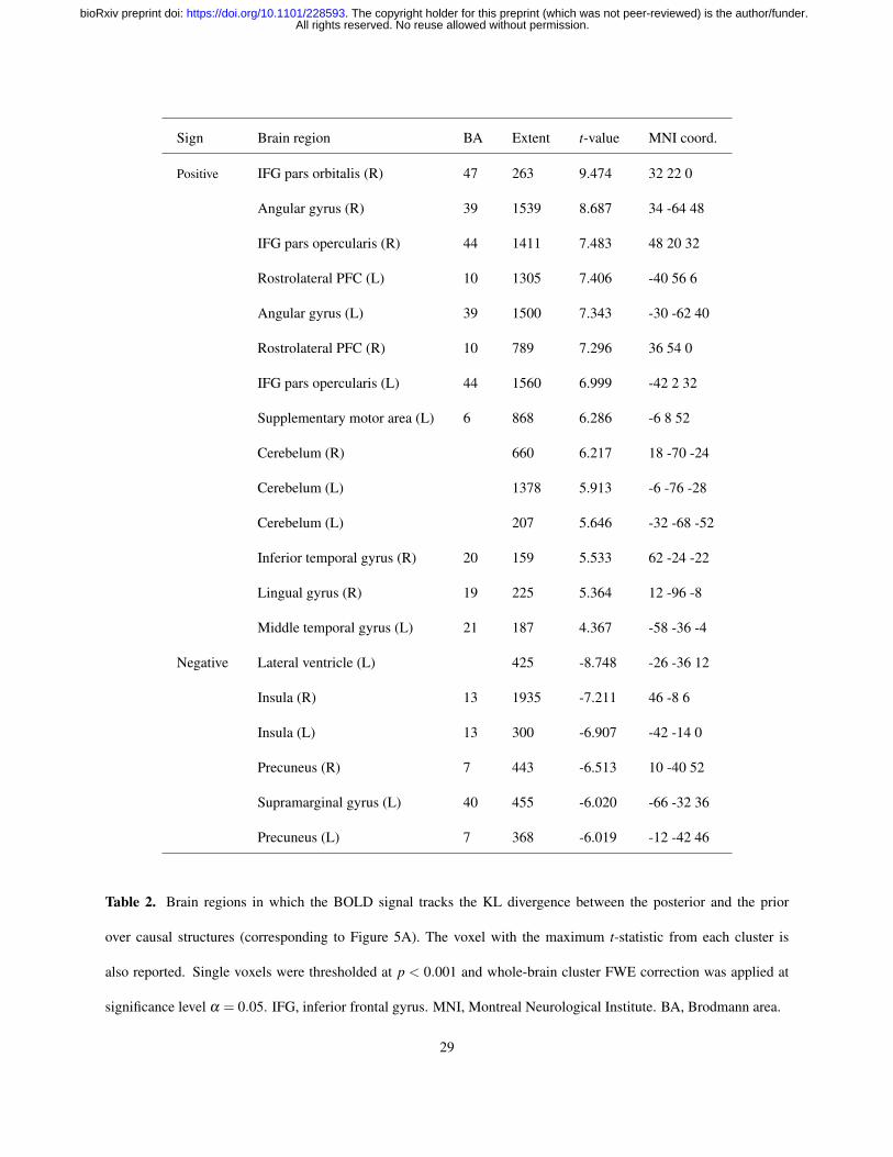
Table 2. Brain regions in which the BOLD signal tracks the KL divergence between the posterior and the prior
over causal structures (corresponding to Figure 5A). The voxel with the maximum t-statistic from each cluster is
also reported. Single voxels were thresholded at p < 0.001 and whole-brain cluster FWE correction was applied at
significance level α = 0.05. IFG, inferior frontal gyrus. MNI, Montreal Neurological Institute. BA, Brodmann area.
29
All rights reserved. No reuse allowed without permission. The copyright holder for this preprint (which was not peer-reviewed) is the author/funder.. https://doi.org/10.1101/228593doi: bioRxiv preprint
Sign Brain region BA Extent t-value MNI coord.
Positive Inferior temporal, parietal,
and occipital gyri (L) 12042 11.091 -50 -52 -16
IFG pars triangularis (R) 45 645 7.935 36 20 26
IFG pars opercularis (L) 44 1663 7.929 -42 6 26
Supplementary motor area (L) 6 1187 7.452 -8 10 50
IFG pars orbitalis 47 181 7.334 30 26 0
Middle temporal gyrus (L) 21 542 6.088 -52 -38 -2
Thalamus and Striatum (R) 421 6.009 12 -14 2
IFG pars orbitalis (L) 47 528 5.269 -40 20 -4
Negative Lateral ventricle (L) 314 -7.449 24 -46 16
Postcentral gyrus (R) 5 390 -6.962 26 -46 62
Lateral ventricle (R) 466 -6.786 -20 -46 12
Precuneus (L) 7 572 -6.261 -26 -48 66
Postcentral gyrus (R) 1 1293 -5.853 60 -12 34
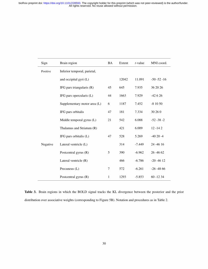
Table 3. Brain regions in which the BOLD signal tracks the KL divergence between the posterior and the prior
distribution over associative weights (corresponding to Figure 5B). Notation and procedures as in Table 2.
30
All rights reserved. No reuse allowed without permission. The copyright holder for this preprint (which was not peer-reviewed) is the author/funder.. https://doi.org/10.1101/228593doi: bioRxiv preprint

Sign Brain region BA Extent t-value MNI coord.
Positive IFG pars orbitalis (R) 47 263 9.474 32 22 0
Angular gyrus (R) 39 1539 8.687 34 -64 48
Rostrolateral PFC (R) 10 746 7.948 36 54 0
Rostrolateral PFC (L) 10 881 7.045 -40 56 6
Angular gyrus (L) 39 1500 7.343 -30 -62 40
Middle frontal gyrus (R) 9 1096 6.666 40 32 22
IFG pars opercularis (L) 44 1049 6.159 -38 14 26
Supplementary motor area (L) 6 543 5.758 -6 8 52
Cerebelum (R) 304 5.498 18 -70 -24
Cerebelum (L) 394 5.417 -8 -78 -30
Cerebelum (L) 165 5.194 -32 -68 -52
Fusiform gyrus (L) 37 206 4.705 -42 -52 -14
Negative Lateral ventricle (L) 327 -8.327 -26 -36 12
Insula (R) 13 937 -6.712 46 -8 6
Insula (L) 13 169 -6.290 -42 -14 0
Supramarginal gyrus (L) 40 298 -5.876 -66 -32 36
Precuneus (R) 7 182 -5.758 10 -40 52
Temporal pole (R) 38 200 -5.419 50 4 -14
Precuneus (L) 7 192 -5.381 -12 -42 46
Table 4. Brain regions in which the BOLD signal is better explained by the causal structures KL divergence than by
the associative weights KL divergence (corresponding to Figure 5C). Notation and procedures as in Table 2.
31
All rights reserved. No reuse allowed without permission. The copyright holder for this preprint (which was not peer-reviewed) is the author/funder.. https://doi.org/10.1101/228593doi: bioRxiv preprint
their structural beliefs, then their test phase performance should more closely resemble the predictions of the structure
learning model, which would be reflected in a high test log likelihood. Thus for a given ROI, a positive correlation
across subjects would indicate that the extent to which that region tracks Bayesian updating during training predicts
the extent to which test performance is consistent with causal structure learning. Importantly, since the KL betas were
estimated on the training trials preceding the test phase, this analysis would yield an unbiased assessment of the neural
predictions.
For each subject and each ROI, we thus obtained a within-subject Pearson correlation coefficient across blocks,
indicating how well the degree to which that ROI encodes structure updating predicts test choices for that subject.
For each ROI, we performed a one-sample t-test against 0 with the Fisher z-transformed Pearson’s r from all subjects
(Figure 5D). We found a significant positive relationship in right angular gyrus (t19 = 2.34, p = 0.03; mean z =
0.21±0.19; peak MNI coordinates [34 -64 48]), left angular gyrus (t19 = 2.53, p = 0.02, mean z = 0.24±0.20; peak
MNI coordinates [-30 -62 40]), and the opercular part of left IFG (t19 = 2.6, p = 0.02, mean z = 0.20± 0.17; peak
MNI coordinates [-42 2 32]). The other regions were not significant (p’s > 0.1). These results link neural variability in
correlates of Bayesian updating to individual variability in test phase choices, providing a more stringent criterion for
identifying the substrates underlying causal structure learning. We performed a similar analysis with the associative
weights KL regressor and found no significant relationship (all p’s > 0.1).
Multivariate representations of the posterior and prior distribution over causal structures
If the brain performs Bayesian inference over causal structures, as our data suggest, then we should be able to identify
regions that contain representations of the full probability distribution over causal structures before and after the
update. We thus performed a whole-brain “searchlight” representational similarity analysis (Kriegeskorte et al., 2008;
Xue et al., 2010; Chan et al., 2016) using 27-voxel spherical searchlights. For each subject, we centered the spherical
ROI on each voxel of the whole-brain volume and computed a representational dissimilarity matrix (RDM) using
the cosine distance between neural activity patterns at trial onset for all pairs of trials (see Materials and Methods).
Intuitively, this RDM reflects which pairs of trials look similar and which pairs of trials look different according to
32
All rights reserved. No reuse allowed without permission. The copyright holder for this preprint (which was not peer-reviewed) is the author/funder.. https://doi.org/10.1101/228593doi: bioRxiv preprint
the neural representations in the area around the given voxel. We then used Spearman’s rank correlation to compare
this neural RDM with a model RDM based on the prior distribution over causal structures. If a given ROI encodes the
prior, then pairs of trials on which the prior is similar would also show similar neural representations, while pairs of
trials on which the prior is different would show differing neural representations. This corresponds to a positive rank
correlation between the model and the neural RDMs.
For each subject and each voxel, we thus obtained a Spearman’s rank correlation coefficient, reflecting the similarity
between activity patterns around that voxel and the prior over causal structures (the representational similarity match).
For each voxel, we then performed a one-sample t-test against 0 with the Fisher z-transformed Spearman’s ρ from all
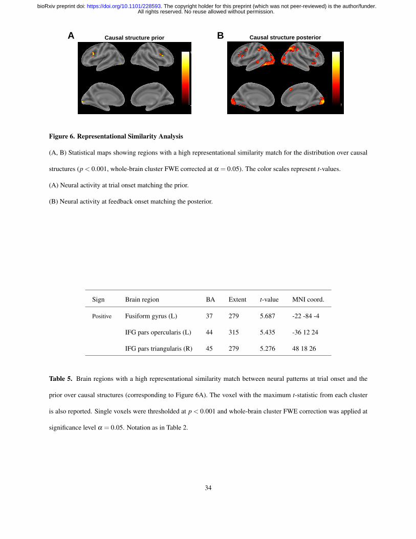
subjects. The resulting t-values from all voxels were used to construct a whole-brain t-map (Figure 6A and Table 5).
This revealed bilateral activations in PFC near the triangular and opercular parts of IFG, as well as a region in left
inferior temporal cortex, suggesting that these areas contain multivariate representations of the prior.
We performed the same analysis using neural activations at feedback onset and the posterior over causal structures
(Figure 6B and Table 6). This revealed a broader set of regions, including a large cluster in visual cortex that extended
bilaterally into inferior temporal cortex and the angular gyri, overlapping with the regions found in the univariate
analyses. We also found bilateral activations near the triangular and opercular parts of IFG, as well as a small cluster
around the orbital part of right IFG. Taken together, these results suggest that the brain maintains representations of
the full probability distribution over causal structures, which it updates in accordance with Bayesian inference on a
trial-by-trial basis as new evidence is accumulated.
33
All rights reserved. No reuse allowed without permission. The copyright holder for this preprint (which was not peer-reviewed) is the author/funder.. https://doi.org/10.1101/228593doi: bioRxiv preprint
Causal structure prior Causal structure posteriorA B
Figure 6. Representational Similarity Analysis
(A, B) Statistical maps showing regions with a high representational similarity match for the distribution over causal
structures (p < 0.001, whole-brain cluster FWE corrected at α = 0.05). The color scales represent t-values.
(A) Neural activity at trial onset matching the prior.
(B) Neural activity at feedback onset matching the posterior.
Sign Brain region BA Extent t-value MNI coord.
Positive Fusiform gyrus (L) 37 279 5.687 -22 -84 -4
IFG pars opercularis (L) 44 315 5.435 -36 12 24
IFG pars triangularis (R) 45 279 5.276 48 18 26
Table 5. Brain regions with a high representational similarity match between neural patterns at trial onset and the
prior over causal structures (corresponding to Figure 6A). The voxel with the maximum t-statistic from each cluster
is also reported. Single voxels were thresholded at p < 0.001 and whole-brain cluster FWE correction was applied at
significance level α = 0.05. Notation as in Table 2.
34
All rights reserved. No reuse allowed without permission. The copyright holder for this preprint (which was not peer-reviewed) is the author/funder.. https://doi.org/10.1101/228593doi: bioRxiv preprint
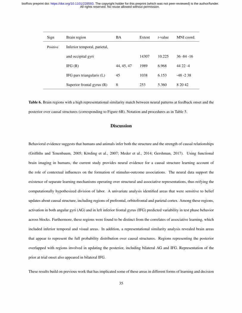
Sign Brain region BA Extent t-value MNI coord.
Positive Inferior temporal, parietal,
and occipital gyri 14307 10.225 36 -84 -16
IFG (R) 44, 45, 47 1989 6.968 44 22 -4
IFG pars triangularis (L) 45 1038 6.153 -48 -2 38
Superior frontal gyrus (R) 8 253 5.360 8 20 42
Table 6. Brain regions with a high representational similarity match between neural patterns at feedback onset and the
posterior over causal structures (corresponding to Figure 6B). Notation and procedures as in Table 5.
Discussion
Behavioral evidence suggests that humans and animals infer both the structure and the strength of causal relationships
(Griffiths and Tenenbaum, 2005; Körding et al., 2007; Meder et al., 2014; Gershman, 2017). Using functional
brain imaging in humans, the current study provides neural evidence for a causal structure learning account of
the role of contextual influences on the formation of stimulus-outcome associations. The neural data support the
existence of separate learning mechanisms operating over structural and associative representations, thus reifying the
computationally hypothesized division of labor. A univariate analysis identified areas that were sensitive to belief
updates about causal structure, including regions of prefrontal, orbitofrontal and parietal cortex. Among these regions,
activation in both angular gyri (AG) and in left inferior frontal gyrus (IFG) predicted variability in test phase behavior
across blocks. Furthermore, these regions were found to be distinct from the correlates of associative learning, which
included inferior temporal and visual areas. In addition, a representational similarity analysis revealed brain areas
that appear to represent the full probability distribution over causal structures. Regions representing the posterior
overlapped with regions involved in updating the posterior, including bilateral AG and IFG. Representation of the
prior at trial onset also appeared in bilateral IFG.
These results build on previous work that has implicated some of these areas in different forms of learning and decision
35
All rights reserved. No reuse allowed without permission. The copyright holder for this preprint (which was not peer-reviewed) is the author/funder.. https://doi.org/10.1101/228593doi: bioRxiv preprint
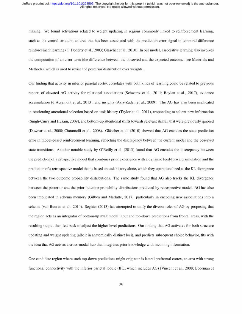
making. We found activations related to weight updating in regions commonly linked to reinforcement learning,
such as the ventral striatum, an area that has been associated with the prediction error signal in temporal difference
reinforcement learning (O’Doherty et al., 2003; Gläscher et al., 2010). In our model, associative learning also involves
the computation of an error term (the difference between the observed and the expected outcome; see Materials and
Methods), which is used to revise the posterior distribution over weights.
Our finding that activity in inferior parietal cortex correlates with both kinds of learning could be related to previous
reports of elevated AG activity for relational associations (Schwartz et al., 2011; Boylan et al., 2017), evidence
accumulation (d’Acremont et al., 2013), and insights (Aziz-Zadeh et al., 2009). The AG has also been implicated
in reorienting attentional selection based on task history (Taylor et al., 2011), responding to salient new information
(Singh-Curry and Husain, 2009), and bottom-up attentional shifts towards relevant stimuli that were previously ignored
(Downar et al., 2000; Ciaramelli et al., 2008). Gläscher et al. (2010) showed that AG encodes the state prediction
error in model-based reinforcement learning, reflecting the discrepancy between the current model and the observed
state transitions. Another notable study by O’Reilly et al. (2013) found that AG encodes the discrepancy between
the prediction of a prospective model that combines prior experience with a dynamic feed-forward simulation and the
prediction of a retrospective model that is based on task history alone, which they operationalized as the KL divergence
between the two outcome probability distributions. The same study found that AG also tracks the KL divergence
between the posterior and the prior outcome probability distributions predicted by retrospective model. AG has also
been implicated in schema memory (Gilboa and Marlatte, 2017), particularly in encoding new associations into a
schema (van Buuren et al., 2014). Seghier (2013) has attempted to unify the diverse roles of AG by proposing that
the region acts as an integrator of bottom-up multimodal input and top-down predictions from frontal areas, with the
resulting output then fed back to adjust the higher-level predictions. Our finding that AG activates for both structure
updating and weight updating (albeit in anatomically distinct loci), and predicts subsequent choice behavior, fits with
the idea that AG acts as a cross-modal hub that integrates prior knowledge with incoming information.
One candidate region where such top-down predictions might originate is lateral prefrontal cortex, an area with strong
functional connectivity with the inferior parietal lobule (IPL, which includes AG) (Vincent et al., 2008; Boorman et
36
All rights reserved. No reuse allowed without permission. The copyright holder for this preprint (which was not peer-reviewed) is the author/funder.. https://doi.org/10.1101/228593doi: bioRxiv preprint
al., 2009). Previous studies on cognitive control (Koechlin et al., 2003; Koechlin and Summerfield, 2007; Badre and
D’Esposito, 2007) have proposed the existence of a functional gradient in lateral PFC, with more anterior regions
encoding representations of progressively higher levels of abstraction, culminating in rlPFC. Donoso et al. (2014)
found evidence that rlPFC performs inference over multiple counterfactual strategies by tracking their reliability,
while the triangular part of IFG is responsible for switching to one of those strategies if the current one is deemed
unreliable. If causal structures are likened to alternative strategies, then these results may relate to our finding
that rlPFC tracks structure updating, while IFG tracks both structure and weight updating. These updates can be
interpreted as discrepancies indicating that the current causal structure and/or its associative weights are unreliable,
thus warranting a revision of the weights or a switch to an alternative causal structure.
Our results also resonate with follow-up work on hierarchical reinforcement learning (Badre et al., 2010; Frank and
Badre, 2012), which extends the notion of a functional hierarchy in lateral PFC to the acquisition of abstract latent
rules that guide stimulus-outcome associations. Frank and Badre (2012) proposed a Bayesian mixture of experts
(MoE) model which arbitrates between hypotheses about stimulus features that are relevant for predicting the outcome,
assigning greater weight to experts that make better predictions. Most pertinent to our study is a model developed by
Collins and Frank (2016) that groups different mappings between stimulus features and responses into distinct task
sets. Different contextual stimuli can elicit different task sets, akin to the occasion-setting function of modulatory
context in our study.
Despite the apparent similarities, there are several notable distinctions between our theoretical framework and those
previous modeling efforts. The term “structure” is used with a different meaning in those studies, either referring to the
hierarchical structure of the hypothesis space (Frank and Badre, 2012), or to the mapping between contextual stimuli
and task sets (Collins and Frank, 2016). While the model of Collins and Frank (2016) can support an infinite number
of task sets, it does not model summation across cues, and therefore cannot represent the additive causal structure
from our study. Some form of summation is widely believed to be important for capturing classic animal learning
phenomena such as blocking, overshadowing, and overexpectation (Rescorla and Wagner, 1972; Soto et al., 2014).
37
All rights reserved. No reuse allowed without permission. The copyright holder for this preprint (which was not peer-reviewed) is the author/funder.. https://doi.org/10.1101/228593doi: bioRxiv preprint

Our results point to potential avenues for future research that could further interrogate the functional role of the regions
we identified. For example, if AG supports causal structure updating, as our data suggest, then temporarily disrupting
it during the first half of training (e.g., using transcranial magnetic stimulation) should result in the same response
pattern on the test trials across all conditions, since subjects would not be able to update their structural beliefs and to
infer different causal structures in the different task conditions. On the other hand, disrupting AG during the second
half of training should have little impact on test responses, as learning has usually plateaued by then. Conversely, if
the areas identified in lateral PFC maintain the full distribution over causal structures, then disrupting them during the
first half of training may slow down learning but would not necessarily result in uniform test responding, as subjects
would still be able to catch up during the second half of training. However, disrupting those regions during the second
half of training could affect the learned distribution over causal structures and result in uniform test response patterns
across all conditions.
An important question that remains open is how structure learning might be implemented in biologically realistic
neural circuits. Tervo et al. (2016) noted the parallels between the hierarchical architecture of cortical circuits and the
hierarchical nature of structure learning, with empirical evidence suggesting that different layers of the hierarchy tend
to be associated with separate cortical circuits. If the brain indeed performs Bayesian inference over causal structures,
this raises the more fundamental question of how ensembles of neurons could represent and perform operations on
probability distributions. Different theories have been put forward, ranging from probabilistic population codes to
Monte Carlo sampling (Pouget et al., 2013). Teasing apart the different possible mechanisms would require developing
behavioral frameworks that lend themselves to computational modeling and quantitative predictions about the inferred
probability distributions (Tervo et al., 2016). We believe this study is an important step in that direction.
In summary, we used a combination of behavioral, neural and computational techniques to tease apart the neural
substrates of structure learning and associative learning. Inference over the space of causal structures recruited
prefrontal regions that have been previously implicated in higher-order reasoning and state representations (rlPFC and
OFC), whereas learning the associative weights activated regions that have been implicated in reward-based learning
(ventral striatum). Both forms of learning elicited bilateral activations in IFG and AG, a region involved in integrating
38
All rights reserved. No reuse allowed without permission. The copyright holder for this preprint (which was not peer-reviewed) is the author/funder.. https://doi.org/10.1101/228593doi: bioRxiv preprint
multimodal sensory input with top-down predictions. Moreover, activity in the voxels that correlated most strongly
with causal structure updating in AG and IFG predicted the similarity between subsequent subject behavior and the
predictions of the causal structure learning model. Finally, representational similarity analysis revealed regions that
encode the full distribution over causal structures: a multivariate signature of the prior was found in IFG, while the
posterior was associated with a broader set of brain areas, including IFG, AG, and inferior temporal cortex. Together,
these results provide strong support for the idea that the brain performs probabilistic inference over latent structures in
the environment, enabling inductive leaps that go beyond the given observations.
Acknowledgements
This research was supported by the National Institutes of Health, award number 1R01MH109177. This work involved
the use of instrumentation supported by the NIH Shared Instrumentation Grant Program grant number S10OD020039.
We acknowledge the University of Minnesota Center for Magnetic Resonance Research for use of the multiband-EPI
pulse sequences. We are grateful to Erik Kastman and Katie Insel for helping to design the experiment and collect the
data.
39
All rights reserved. No reuse allowed without permission. The copyright holder for this preprint (which was not peer-reviewed) is the author/funder.. https://doi.org/10.1101/228593doi: bioRxiv preprint
References
Amiez C, Joseph JP, Procyk E (2005) Anterior cingulate error-related activity is modulated by predicted reward.
European Journal of Neuroscience 21:3447–3452.
Amiez C, Sallet J, Procyk E, Petrides M (2012) Modulation of feedback related activity in the rostral anterior
cingulate cortex during trial and error exploration. NeuroImage 63:1078 – 1090.
Aziz-Zadeh L, Kaplan JT, Iacoboni M (2009) “aha!”: The neural correlates of verbal insight solutions. Human Brain
Mapping 30:908–916.
Badre D, D’Esposito M (2007) Functional magnetic resonance imaging evidence for a hierarchical organization of
the prefrontal cortex. Journal of Cognitive Neuroscience 19:2082–2099.
Badre D, Doll BB, Long NM, Frank MJ (2012) Rostrolateral prefrontal cortex and individual differences in
uncertainty-driven exploration. Neuron 73:595 – 607.
Badre D, Kayser AS, D’Esposito M (2010) Frontal cortex and the discovery of abstract action rules.
Neuron 66:315–326.
Balaz MA, Capra S, Hartl P, Miller RR (1981) Contextual potentiation of acquired behavior after devaluing direct
context-us associations. Learning and Motivation 12:383–397.
Balsam P, Tomie A (1985) Context and Learning Psychology Press.
Bell A, Summerfield C, Morin E, Malecek N, Ungerleider L (2016) Encoding of stimulus probability in macaque
inferior temporal cortex. Current Biology 26:2280–2290.
Boorman ED, Behrens TE, Rushworth MF (2011) Counterfactual choice and learning in a neural network centered
on human lateral frontopolar cortex. PLoS Biol 9:e1001093 PBIOLOGY-D-10-00233[PII].
Boorman ED, Behrens TE, Woolrich MW, Rushworth MF (2009) How green is the grass on the other side?
frontopolar cortex and the evidence in favor of alternative courses of action. Neuron 62:733 – 743.
40
All rights reserved. No reuse allowed without permission. The copyright holder for this preprint (which was not peer-reviewed) is the author/funder.. https://doi.org/10.1101/228593doi: bioRxiv preprint
Bouton ME, Bolles R (1993) Contextual control of the extinction of conditioned fear. Learning and
Motivation 10:445–466.
Bouton ME, King DA (1983) Contextual control of the extinction of conditioned fear: Tests for the associative value
of the context. Journal of Experimental Psychology: Animal Behavior Processes 9:248–265.
Bouton ME, Peck CA (1989) Context effects on conditioning, extinction, and reinstatement in an appetitive
conditioning preparation. Animal Learning & Behavior 17:188–198.
Boylan C, Trueswell JC, Thompson-Schill SL (2017) Relational vs. attributive interpretation of nominal compounds
differentially engages angular gyrus and anterior temporal lobe. Brain and Language 169:8 – 21.
Braun DA, Mehring C, Wolpert DM (2010) Structure learning in action. Behavioural Brain Research 206:157 – 165.
Brown JW, Braver TS (2005) Learned predictions of error likelihood in the anterior cingulate cortex.
Science 307:1118–1121.
Bush G, Vogt BA, Holmes J, Dale AM, Greve D, Jenike MA, Rosen BR (2002) Dorsal anterior cingulate cortex: A
role in reward-based decision making. Proceedings of the National Academy of Sciences 99:523–528.
Chan SCY, Niv Y, Norman KA (2016) A probability distribution over latent causes, in the orbitofrontal cortex.
Journal of Neuroscience 36:7817–7828.
Christoff K, Keramatian K, Gordon AM, Smith R, Mädler B (2009) Prefrontal organization of cognitive control
according to levels of abstraction. Brain Research 1286:94 – 105.
Christoff K, Prabhakaran V, Dorfman J, Zhao Z, Kroger JK, Holyoak KJ, Gabrieli JD (2001) Rostrolateral prefrontal
cortex involvement in relational integration during reasoning. NeuroImage 14:1136 – 1149.
Ciaramelli E, Grady CL, Moscovitch M (2008) Top-down and bottom-up attention to memory: A hypothesis (atom)
on the role of the posterior parietal cortex in memory retrieval. Neuropsychologia 46:1828 – 1851 Part Special Issue:
What is the Parietal Lobe Contribution to Human Memory?
41
All rights reserved. No reuse allowed without permission. The copyright holder for this preprint (which was not peer-reviewed) is the author/funder.. https://doi.org/10.1101/228593doi: bioRxiv preprint

Collins AGE, Frank MJ (2016) Motor demands constrain cognitive rule structures. PLOS Computational
Biology 12:1–17.
Collins AG, Cavanagh JF, Frank MJ (2014) Human eeg uncovers latent generalizable rule structure during learning.
Journal of Neuroscience 34:4677–4685.
Cousineau D (2005) Confidence intervals in within-subject designs: A simpler solution to loftus and masson?s
method. Tutorials in Quantitative Methods for Psychology 1:42 – 45.
Crone EA, Wendelken C, Van Leijenhorst L, Honomichl RD, Christoff K, Bunge SA (2009) Neurocognitive
development of relational reasoning. Developmental Science 12:55–66.
d’Acremont M, Fornari E, Bossaerts P (2013) Activity in inferior parietal and medial prefrontal cortex
signals the accumulation of evidence in a probability learning task. PLoS Comput Biol 9:e1002895
PCOMPBIOL-D-12-01046[PII].
Davis T, Goldwater M, Giron J (2017) From concrete examples to abstract relations: The rostrolateral prefrontal
cortex integrates novel examples into relational categories. Cerebral Cortex 27:2652.
Daw ND, O’Doherty JP, Dayan P, Seymour B, Dolan RJ (2006) Cortical substrates for exploratory decisions in
humans. Nature 441:876–879.
Dayan P, Kakade S (2000) Explaining away in weight space In Proceedings of the 13th International Conference on
Neural Information Processing Systems, NIPS’00, pp. 430–436, Cambridge, MA, USA. MIT Press.
Desikan RS, Ségonne F, Fischl B, Quinn BT, Dickerson BC, Blacker D, Buckner RL, Dale AM, Maguire RP, Hyman
BT, Albert MS, Killiany RJ (2006) An automated labeling system for subdividing the human cerebral cortex on mri
scans into gyral based regions of interest. NeuroImage 31:968 – 980.
Desmond JE, Glover GH (2002) Estimating sample size in functional mri (fmri) neuroimaging studies: Statistical
power analyses. Journal of Neuroscience Methods 118:115 – 128.
42
All rights reserved. No reuse allowed without permission. The copyright holder for this preprint (which was not peer-reviewed) is the author/funder.. https://doi.org/10.1101/228593doi: bioRxiv preprint

Dickinson A (2001) The 28th bartlett memorial lecture causal learning: An associative analysis. The Quarterly
Journal of Experimental Psychology Section B 54:3–25 PMID: 11216300.
Domenech P, Koechlin E (2015) Executive control and decision-making in the prefrontal cortex. Current Opinion in
Behavioral Sciences 1:101 – 106 Cognitive control.
Donoso M, Collins AGE, Koechlin E (2014) Foundations of human reasoning in the prefrontal cortex.
Science 344:1481–1486.
Downar J, Crawley AP, Mikulis DJ, Davis KD (2000) A multimodal cortical network for the detection of changes in
the sensory environment. Nat Neurosci 3:277–283.
Dunsmoor JE, Niv Y, Daw N, Phelps EA (2015) Rethinking extinction. Neuron 88:47–63.
Eickhoff SB, Stephan KE, Mohlberg H, Grefkes C, Fink GR, Amunts K, Zilles K (2005) A new spm toolbox for
combining probabilistic cytoarchitectonic maps and functional imaging data. NeuroImage 25:1325 – 1335.
Feinberg DA, Moeller S, Smith SM, Auerbach E, Ramanna S, Gunther M, Glasser MF, Miller KL, Ugurbil K,
Yacoub E (2010) Multiplexed echo planar imaging for sub-second whole brain FMRI and fast diffusion imaging.
PLoS ONE 5:e15710.
Fletcher PC, Anderson JM, Shanks DR, Honey R, Carpenter TA, Donovan T, Papadakis N, Bullmore ET (2001)
Responses of human frontal cortex to surprising events are predicted by formal associative learning theory. Nat
Neurosci 4:1043–1048.
Frank MJ, Badre D (2012) Mechanisms of hierarchical reinforcement learning in corticostriatal circuits 1:
Computational analysis. Cerebral Cortex 22:509–526.
Gershman SJ (2015) A unifying probabilistic view of associative learning. PLoS Comput Biol 11:e1004567
PCOMPBIOL-D-15-00974[PII].
Gershman SJ (2017) Context-dependent learning and causal structure. Psychonomic Bulletin and
Review 24:557–565.
43
All rights reserved. No reuse allowed without permission. The copyright holder for this preprint (which was not peer-reviewed) is the author/funder.. https://doi.org/10.1101/228593doi: bioRxiv preprint
Gershman SJ, Niv Y (2010) Learning latent structure: Carving nature at its joints. Curr Opin Neurobiol 20:251–256
20227271[pmid].
Gershman SJ, Norman KA, Niv Y (2015) Discovering latent causes in reinforcement learning. Current Opinion in
Behavioral Sciences 5:43 – 50 Neuroeconomics.
Gershman SJ, Pesaran B, Daw ND (2009) Human reinforcement learning subdivides structured action spaces by
learning effector-specific values. Journal of Neuroscience 29:13524–13531.
Gilboa A, Marlatte H (2017) Neurobiology of schemas and schema-mediated memory. Trends in Cognitive Sciences .
Gläscher J (2009) Visualization of group inference data in functional neuroimaging. Neuroinformatics 7:73–82.
Gläscher J, Daw N, Dayan P, O’Doherty JP (2010) States versus rewards: Dissociable neural prediction error signals
underlying model-based and model-free reinforcement learning. Neuron 66:585 – 595.
Goodman N, Ullman T, Tenenbaum J (2011) Learning a theory of causality. Psychological Review 118:110–119.
Grahame NJ, Hallam SC, Geier L, Miller RR (1990) Context as an occasion setter following either cs acquisition
and extinction or cs acquisition alone. Learning and Motivation 21:237–265.
Grau JW, Rescorla RA (1984) Role of context in autoshaping. Journal of Experimental Psychology: Animal Behavior
Processes 10:324–332.
Greve DN (2002) Optseq2 home page.
Griffiths TL, Tenenbaum JB (2005) Structure and strength in causal induction. Cognitive Psychology 51:334 – 384.
Holroyd CB, Coles MGH (2002) The neural basis of human error processing: Reinforcement learning, dopamine,
and the error-related negativity. Psychological Review 109:679–709.
Hung CP, Kreiman G, Poggio T, DiCarlo JJ (2005) Fast readout of object identity from macaque inferior temporal
cortex. Science 310:863–866.
44
All rights reserved. No reuse allowed without permission. The copyright holder for this preprint (which was not peer-reviewed) is the author/funder.. https://doi.org/10.1101/228593doi: bioRxiv preprint
Jackson SAW, Horst NK, Pears A, Robbins TW, Roberts AC (2016) Role of the perigenual anterior cingulate and
orbitofrontal cortex in contingency learning in the marmoset. Cereb Cortex 26:3273–3284 bhw067[PII].
Kakade S, Dayan P (2002) Acquisition and extinction in autoshaping. Psychological review 109:533–44.
Kaye H, Preston GC, Szabo L, Druiff H, Mackintosh NJ (1987) Context specificity of conditioning and latent
inhibition: Evidence for a dissociation of latent inhibition and associative interference. The Quarterly Journal of
Experimental Psychology Section B 39:127–145.
Kemp C, Perfors A, Tenenbaum JB (2007) Learning overhypotheses with hierarchical bayesian models.
Developmental Science 10:307–321.
Kennerley SW, Walton ME, Behrens TEJ, Buckley MJ, Rushworth MFS (2006) Optimal decision making and the
anterior cingulate cortex. Nat Neurosci 9:940–947.
Koechlin E, Ody C, Kouneiher F (2003) The architecture of cognitive control in the human prefrontal cortex.
Science 302:1181–1185.
Koechlin E, Summerfield C (2007) An information theoretical approach to prefrontal executive function. Trends in
Cognitive Sciences 11:229–235.
Körding KP, Beierholm U, Ma WJ, Quartz S, Tenenbaum JB, Shams L (2007) Causal inference in multisensory
perception. PLoS One 2:e943.
Kriegeskorte N, Mur M, Bandettini P (2008) Representational similarity analysis – connecting the branches of
systems neuroscience. Frontiers in Systems Neuroscience 2.
Kruschke JK (2008) Bayesian approaches to associative learning: From passive to active learning. Learning &
Behavior 36:210–226.
Lovibond PF, Preston G, Mackintosh N (1984) Context specificity of conditioning, extinction, and latent inhibition.
Journal of Experimental Psychology: Animal Behavior Processes 10:360–375.
45
All rights reserved. No reuse allowed without permission. The copyright holder for this preprint (which was not peer-reviewed) is the author/funder.. https://doi.org/10.1101/228593doi: bioRxiv preprint
MacDonald AW, Cohen JD, Stenger VA, Carter CS (2000) Dissociating the role of the dorsolateral prefrontal and
anterior cingulate cortex in cognitive control. Science 288:1835–1838.
Madarasz TJ, Diaz-Mataix L, Akhand O, Ycu EA, LeDoux JE, Johansen JP (2016) Evaluation of ambiguous
associations in the amygdala by learning the structure of the environment. Nature Neuroscience 19:965–972.
Meder B, Mayrhofer R, Waldmann MR (2014) Structure induction in diagnostic causal reasoning. Psychological
Review 121:277–301.
Meyer T, Olson CR (2011) Statistical learning of visual transitions in monkey inferotemporal cortex. Proceedings of
the National Academy of Sciences 108:19401–19406.
Meyers EM, Freedman DJ, Kreiman G, Miller EK, Poggio T (2008) Dynamic population coding of category
information in inferior temporal and prefrontal cortex. Journal of Neurophysiology 100:1407–1419.
Miller RR, Barnet RC, Grahame NJ (1995) Assessment of the Rescorla-Wagner model. Psychological
Bulletin 117:363–386.
Moeller S, Yacoub E, Olman CA, Auerbach E, Strupp J, Harel N, U?urbil K (2010) Multiband multislice GE-EPI
at 7 tesla, with 16-fold acceleration using partial parallel imaging with application to high spatial and temporal
whole-brain fMRI. Magn Reson Med 63:1144–1153.
Nogueira R, Abolafia JM, Drugowitsch J, Balaguer-Ballester E, Sanchez-Vives MV, Moreno-Bote R (2017) Lateral
orbitofrontal cortex anticipates choices and integrates prior with current information. Nature 8:14823 EP – Article.
Noonan MP, Kolling N, Walton ME, Rushworth MFS (2012) Re-evaluating the role of the orbitofrontal cortex in
reward and reinforcement. European Journal of Neuroscience 35:997–1010.
Noonan MP, Mars RB, Rushworth MFS (2011) Distinct roles of three frontal cortical areas in reward-guided behavior.
Journal of Neuroscience 31:14399–14412.
46
All rights reserved. No reuse allowed without permission. The copyright holder for this preprint (which was not peer-reviewed) is the author/funder.. https://doi.org/10.1101/228593doi: bioRxiv preprint
Noonan MP, Walton ME, Behrens TEJ, Sallet J, Buckley MJ, Rushworth MFS (2010) Separate value comparison
and learning mechanisms in macaque medial and lateral orbitofrontal cortex. Proceedings of the National Academy
of Sciences 107:20547–20552.
Odling-Smee F (1978) The overshadowing of background stimuli: some effects of varying amounts of training and
UCS intensity. The Quarterly Journal of Experimental Psychology 30:737–746.
O’Doherty JP, Dayan P, Friston K, Critchley H, Dolan RJ (2003) Temporal difference models and reward-related
learning in the human brain. Neuron 38:329 – 337.
O’Reilly JX, Jbabdi S, Rushworth MFS, Behrens TEJ (2013) Brain systems for probabilistic and dynamic prediction:
Computational specificity and integration. PLoS Biol 11:e1001662 PBIOLOGY-D-13-01872[PII].
Pearce JM, Bouton ME (2001) Theories of associative learning in animals. Annual Review of Psychology 52:111–139.
Peirce JW (2007) Psychopy-psychophysics software in python. Journal of Neuroscience Methods 162:8 – 13.
Pouget A, Beck JM, Ma WJ, Latham PE (2013) Probabilistic brains: knowns and unknowns. Nat
Neurosci 16:1170–1178 Review.
Prabhakaran V, Smith JA, Desmond JE, Glover GH, Gabrieli JD (1997) Neural substrates of fluid reasoning:
An fmri study of neocortical activation during performance of the raven’s progressive matrices test. Cognitive
Psychology 33:43 – 63.
Preston G, Dickinson A, Mackintosh N (1986) Contextual conditional discriminations. The Quarterly Journal of
Experimental Psychology 38:217–237.
Rescorla RA, Wagner AR (1972) A theory of Pavlovian conditioning: Variations on the effectiveness of
reinforcement and non-reinforcement In Black AH, Prokasy WF, editors, Classical conditioning II: Current research
and theory, pp. 64–99. Appleton-Century-Crofts, New York.
Rigoux L, Stephan K, Friston K, Daunizeau J (2014) Bayesian model selection for group studies - revisited.
NeuroImage 84:971 – 985.
47
All rights reserved. No reuse allowed without permission. The copyright holder for this preprint (which was not peer-reviewed) is the author/funder.. https://doi.org/10.1101/228593doi: bioRxiv preprint
Rolls ET, Joliot M, Tzourio-Mazoyer N (2015) Implementation of a new parcellation of the orbitofrontal cortex in
the automated anatomical labeling atlas. NeuroImage 122:1 – 5.
Rudebeck PH, Murray EA (2011a) Balkanizing the primate orbitofrontal cortex: distinct subregions for comparing
and contrasting values. Annals of the New York Academy of Sciences 1239:1–13.
Rudebeck PH, Murray EA (2011b) Dissociable effects of subtotal lesions within the macaque orbital prefrontal
cortex on reward-guided behavior. Journal of Neuroscience 31:10569–10578.
Schuck NW, Cai MB, Wilson RC, Niv Y (2016) Human orbitofrontal cortex represents a cognitive map of state
space. Neuron 91:1402–1412.
Schultz W, Dayan P, Montague PR (1997) A neural substrate of prediction and reward. Science 275:1593–1599.
Schwartz MF, Kimberg DY, Walker GM, Brecher A, Faseyitan OK, Dell GS, Mirman D, Coslett HB (2011)
Neuroanatomical dissociation for taxonomic and thematic knowledge in the human brain. Proc Natl Acad Sci U
S A 108:8520–8524 201014935[PII].
Schwarz G (1978) Estimating the dimension of a model. Ann. Statist. 6:461–464.
Seghier ML (2013) The angular gyrus. The Neuroscientist 19:43–61 PMID: 22547530.
Shenhav A, Cohen JD, Botvinick MM (2016) Dorsal anterior cingulate cortex and the value of control. Nat
Neurosci 19:1286–1291 Perspective.
Silvetti M, Vassena E, Verguts T (2017) Dorsal anterior cingulate-midbrain ensemble as a reinforcement meta-learner.
bioRxiv .
Singh-Curry V, Husain M (2009) The functional role of the inferior parietal lobe in the dorsal and ventral stream
dichotomy. Neuropsychologia 47:1434 – 1448 Perception and Action.
Soto FA, Gershman SJ, Niv Y (2014) Explaining compound generalization in associative and causal learning through
rational principles of dimensional generalization. Psychological Review 121:526–558.
48
All rights reserved. No reuse allowed without permission. The copyright holder for this preprint (which was not peer-reviewed) is the author/funder.. https://doi.org/10.1101/228593doi: bioRxiv preprint
Sul JH, Kim H, Huh N, Lee D, Jung MW (2010) Distinct roles of rodent orbitofrontal and medial prefrontal cortex
in decision making. Neuron 66:449–460.
Swartzentruber D (1995) Modulatory mechanisms in pavlovian conditioning. Animal Learning &
Behavior 23:123–143.
Swartzentruber D, Bouton ME (1986) Analysis of the associative and occasion setting properties of
contexts participating in a pavlovian discrimination. Journal of Experimental Psychology: Animal Behavior
Processes 12:333–350.
Takenouchi K, Nishijo H, Uwano T, Tamura R, Takigawa M, Ono T (1999) Emotional and behavioral correlates of
the anterior cingulate cortex during associative learning in rats. Neuroscience 93:1271 – 1287.
Taylor PCJ, Muggleton NG, Kalla R, Walsh V, Eimer M (2011) Tms of the right angular gyrus modulates priming
of pop-out in visual search: combined tms-erp evidence. Journal of Neurophysiology 106:3001–3009.
Tervo DG, Hwang BY, Viswanathan S, Gaj T, Lavzin M, Ritola K, Lindo S, Michael S, Kuleshova E, Ojala D, Huang
CC, Gerfen C, Schiller J, Dudman J, Hantman A, Looger L, Schaffer D, Karpova A (2017) A designer aav variant
permits efficient retrograde access to projection neurons. Neuron 92:372–382.
Tervo DGR, Tenenbaum JB, Gershman SJ (2016) Toward the neural implementation of structure learning. Current
Opinion in Neurobiology 37:99 – 105 Neurobiology of cognitive behavior.
Tzourio-Mazoyer N, Landeau B, Papathanassiou D, Crivello F, Etard O, Delcroix N, Mazoyer B, Joliot M (2002)
Automated anatomical labeling of activations in spm using a macroscopic anatomical parcellation of the mni mri
single-subject brain. NeuroImage 15:273 – 289.
van Buuren M, Kroes MC, Wagner IC, Genzel L, Morris RG, Fernández G (2014) Initial investigation
of the effects of an experimentally learned schema on spatial associative memory in humans. Journal of
Neuroscience 34:16662–16670.
van der Kouwe AJ, Benner T, Salat DH, Fischl B (2008) Brain morphometry with multiecho mprage.
NeuroImage 40:559 – 569.
49
All rights reserved. No reuse allowed without permission. The copyright holder for this preprint (which was not peer-reviewed) is the author/funder.. https://doi.org/10.1101/228593doi: bioRxiv preprint
Vincent JL, Kahn I, Snyder AZ, Raichle ME, Buckner RL (2008) Evidence for a frontoparietal control system
revealed by intrinsic functional connectivity. Journal of Neurophysiology 100:3328–3342.
Wendelken C, Bunge SA (2010) Transitive inference: Distinct contributions of rostrolateral prefrontal cortex and the
hippocampus. Journal of Cognitive Neuroscience 22:837–847 PMID: 19320546.
Wendelken C, Chung D, Bunge SA (2012) Rostrolateral prefrontal cortex: Domain-general or domain-sensitive?
Human Brain Mapping 33:1952–1963.
Wendelken C, Nakhabenko D, Donohue SE, Carter CS, Bunge SA (2008) “brain is to thought as stomach is
to ??”: Investigating the role of rostrolateral prefrontal cortex in relational reasoning. Journal of Cognitive
Neuroscience 20:682–693.
Wendelken C, O’Hare ED, Whitaker KJ, Ferrer E, Bunge SA (2011) Increased functional selectivity over
development in rostrolateral prefrontal cortex. Journal of Neuroscience 31:17260–17268.
Wilson R, Takahashi Y, Schoenbaum G, Niv Y (2013) Orbitofrontal cortex as a cognitive map of task space.
Neuron 81:267–279.
Xu J, Moeller S, Auerbach EJ, Strupp J, Smith SM, Feinberg DA, Yacoub E, U?urbil K (2013) Evaluation of slice
accelerations using multiband echo planar imaging at 3 T. Neuroimage 83:991–1001.
Xue G, Dong Q, Chen C, Lu Z, Mumford JA, Poldrack RA (2010) Greater neural pattern similarity across repetitions
is associated with better memory. Science 330:97–101.
Zajkowski WK, Kossut M, Wilson RC (2017) A causal role for right frontopolar cortex in directed, but not random,
exploration. bioRxiv .
50
All rights reserved. No reuse allowed without permission. The copyright holder for this preprint (which was not peer-reviewed) is the author/funder.. https://doi.org/10.1101/228593doi: bioRxiv preprint


![Conceptual Confusions and Causal Dynamics Lo Presti, Patrizio · PATrIzIO LO PrESTI and that “recording […] is the principle underlying social normativity as a whole” (2018,](https://static.fdocuments.net/doc/165x107/5f625b5fe936e5079c6f951b/conceptual-confusions-and-causal-dynamics-lo-presti-patrizio-patrizio-lo-presti.jpg)