Neural coding and feature extraction of time-varying signals
243
Neural coding and feature extraction of time-varying signals Thesis by Gabriel Kreiman In partial fulfillment of the requirements for the degree of (Master of Science) California Institute of Technology Pasadena, California 2002
Transcript of Neural coding and feature extraction of time-varying signals
Neural coding and feature extraction
of time-varying signals
Thesis by
Gabriel Kreiman
In partial fulfillment of the requirements
for the degree of
(Master of Science)
California Institute of Technology
Pasadena, California
2002

ii
To Tobias Shlomo Kreiman
iii
Abstract
What are the neuronal codes that the brain uses to represent information? This
constitutes one of the most fascinating and challenging questions in Neuroscience. Here
we report the results of our investigations about the mechanisms of stimulus encoding
and feature extraction using the weakly electric fish Eigenmannia as a model. In many
circumstances, sensory systems are subject to natural stimuli that are constantly
changing. Therefore we decided to study the representation of time varying signals.
Eigenmannia constitutes an ideal system to combine neurophysiological and
computational techniques to study neural coding. We have characterized the variability of
neuronal responses with a new approach by using parameterized distances between spike
trains defined by Victor and Purpura. This measure of variability is widely applicable to
neuronal responses, irrespective of the type of stimuli used (deterministic versus random)
or the reliability of the recorded spike trains. We also quantitatively defined and
evaluated the robustness of the neural code to spike time jittering, spike failures and
spontaneous spikes. Our data show that the intrinsic variability of single spike trains lies
outside of the range where it might degrade the information conveyed, yet still allows for
improvement in coding by averaging across multiple afferent fibers. We also built a
phenomenological model of P-receptor afferents incorporating both their linear transfer
properties and the variability of their spike trains. We then studied the extraction of
features from the time varying signal by bursts of spikes of multiple pyramidal cells, the
next stage of information processing. To address the question of whether correlated
responses of nearby neurons within topographic sensory maps are merely a sign of

iv
redundancy or carry additional information we recorded simultaneously from pairs of
electrosensory pyramidal cells with overlapping receptive fields in the hindbrain of
weakly electric fish. We found that nearby pyramidal cells exhibit strong stimulus-
induced correlations. The detailed stimulus encoding by pairs of pyramidal cells was
inferior to that from single primary afferents. However, the detection of coincident bursts
of activity could significantly enhance the extraction of upstrokes and downstrokes in the
stimulus amplitude. Our investigations reveal mechanisms by which the nervous system
can accurately and robustly transduce a time-varying signal into a digital spike train and
then extract behaviorally relevant features.

v
Acknowledgments
All the work described in the following pages would not have been possible
without the collaboration and help from an encouraging group of friends and colleagues.
Fabrizio Gabbiani has had the kindness and patience to guide me through the first steps in
the quantitative study of spike trains and how action potentials encode information. He
was the pioneer on the theoretical side of the explorations of neural coding in the electric
fish and all the work here described constitutes his legacy. He has been a constant source
of wisdom and encouragement.
None of the work described in these pages would have been feasible without the
laborious and rigorous enterprise of Walter Metzner and Rüdiger Krahe. From the warm
realm of Riverside and more recently from UCLA they have bred the fish, designed the
experiments, inserted the electrodes and chased the neurons. This has been a marvelous
collaborative effort where experimentalists and theoreticians could join, speak the same
language and work together towards a common goal. Walter Metzner and Rüdiger Krahe
have been patient and attentive when I repeatedly and eagerly asked for more data and
they have encouraged and prompted me to look at the results in different ways, to pose
new and distinct questions and to sit on the side of the fish to try to understand what is
going on.
A number of people have been very kind in providing us with excellent feedback,
and reading and reviewing our drafts including Amit Manwani, Mark Stopfer, Mark
Konishi, Mariela Zirlinger and Len Maler. Len Maler has been a constant source of

vi
advice; in particular, his advice was very helpful to carry out the histological procedure
described in Chapter 3.
I would also like to acknowledge the constant help from my family including
Raul, Lidia, Lauri, Mariela, Tobias, Elias, Haydee, Dora, Machi and Mati. While I am
quite sure that they still do not comprehend what researching the neural codes in electric
fish means, their continuous support has been fundamental for the completion of all this
work.
My advisor, Christof Koch, has been extremely kind and encouraging throughout
these years. Every single conversation with him has left my mind with a myriad of new
questions and new paths to explore. His enthusiasm and scientific curiosity is contagious
and imparts everyone around him with a strong momentum to pursue original and
challenging problems. He has constantly shown me new ways to look at the experiments,
the theories, and the big picture behind the scenes of how the brain works.

Gabriel Kreiman Thesis vii
Table of Contents
Abstract .............................................................................................................................. iii
Acknowledgments............................................................................................................... v
Table of Contents.............................................................................................................. vii
List of Figures .................................................................................................................... xi
List of Tables ................................................................................................................... xiv
List of Tables ................................................................................................................... xiv
1 The investigation of neuronal codes ................................................................................ 1
1.1 What is a neuronal code? .......................................................................................... 1
1.2 Organization of the Thesis........................................................................................ 2
1.3 Brief history of inquires into neural coding.............................................................. 5
1.4 Eigenmannia as a model ........................................................................................... 7
1.5 Introduction to some of the methods ...................................................................... 10
1.5.1 Stimulus ........................................................................................................... 11
1.5.2 Electrophysiological recordings....................................................................... 12
1.5.3 Stimulus reconstruction ................................................................................... 14
1.5.4 Feature extraction............................................................................................. 20
1.5.5 Bursting............................................................................................................ 23
1.6 What would it mean to understand the neuronal code? .......................................... 24
1.7 Figure legends......................................................................................................... 26
2 Robustness, Variability and Modeling of P-receptor afferents spike trains .................. 34
2.1 Overview................................................................................................................. 34

Gabriel Kreiman Thesis viii
2.2 Introduction............................................................................................................. 35
2.3 Methods .................................................................................................................. 38
2.3.1 Preparation and electrophysiology................................................................... 38
2.3.2 Stimulation....................................................................................................... 38
2.3.3 Characterization of spike train variability........................................................ 40
2.3.4 Stimulus estimation........................................................................................ 46
2.3.5 Robustness of RAM encoding to spike time jitter, and random spike additions
or deletions................................................................................................................ 48
2.3.6 Modeling of P-receptor afferent spike trains ................................................... 50
2.4 Results..................................................................................................................... 53
2.4.1 Responses of P-receptors to repeated presentations of identical RAMs.......... 53
2.4.2 Quantification of response variability.............................................................. 54
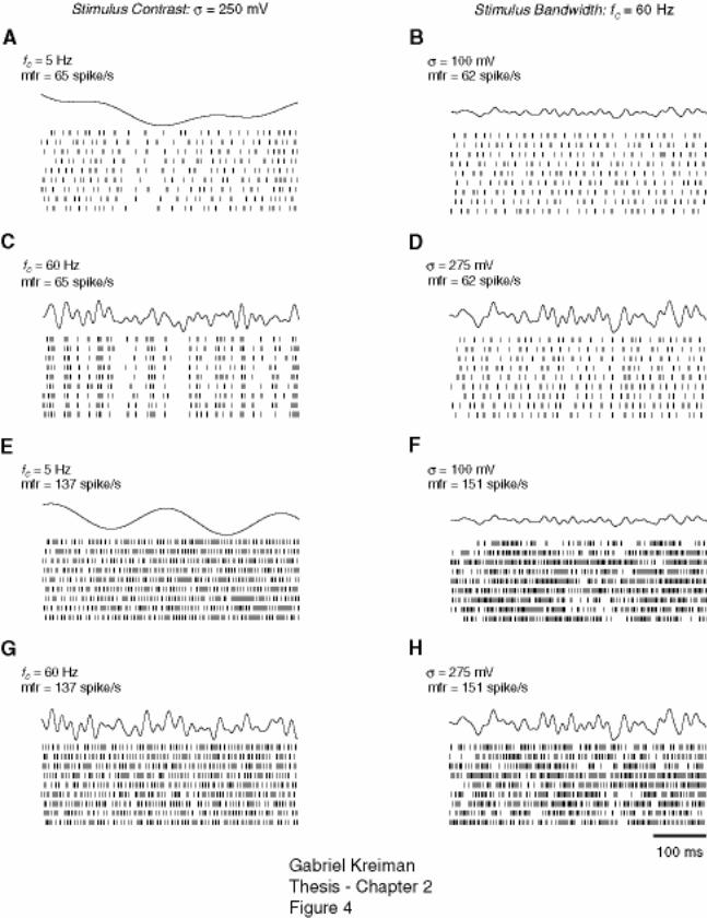
2.4.3 Dependence of temporal jitter on stimulus cut-off frequency ......................... 59
2.4.4 Variability and stimulus contrast ..................................................................... 60
2.4.5 Robustness of stimulus encoding..................................................................... 61
2.4.6 Modeling of P-receptor afferent variability and linear transfer properties ...... 62
2.5 Discussion............................................................................................................... 64
2.5.1 Quantification of spike train variability ........................................................... 64
2.5.2 Variability under various stimulus conditions ................................................. 67
2.5.3 Variability and robustness of encoding............................................................ 68
2.5.4 Variability and the processing of amplitude modulations in the ELL ............. 69
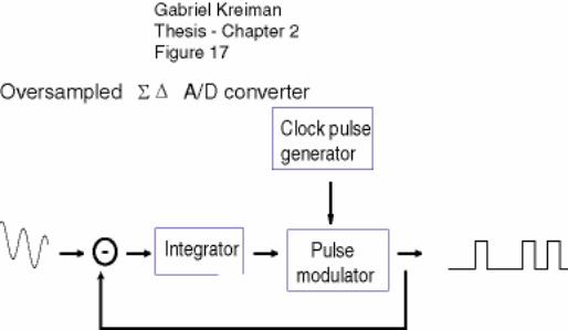
2.5.5 Encoding of biological signals and analog to digital conversion..................... 71
2.6 Tables...................................................................................................................... 73

Gabriel Kreiman Thesis ix
2.7 Figure legends......................................................................................................... 74
3 Stimulus encoding and feature extraction by multiple sensory neurons...................... 100
3.1 Overview............................................................................................................... 100
3.2 Introduction........................................................................................................... 101
3.3 Methods ................................................................................................................ 103
3.3.1 Preparation and electrophysiology................................................................. 103
3.3.2 Anatomy......................................................................................................... 104
3.3.3 Stimulation..................................................................................................... 105
3.3.4 Cross-correlations .......................................................................................... 106
3.3.5 Stimulus reconstruction ................................................................................. 108
3.3.6 Feature extraction........................................................................................... 110
3.4 Results................................................................................................................... 113
3.4.1 Characteristics of correlated activity in ELL pyramidal cells........................ 114
3.4.2 Encoding of the time course of RAMs........................................................... 116
3.4.3 Feature extraction by multiple pyramidal cells.............................................. 118
3.4.4 Terminal spread of single primary afferents .................................................. 120
3.5 Discussion............................................................................................................. 121
3.5.1 Source of correlated activity .......................................................................... 121
3.5.2 Encoding of stimulus time course.................................................................. 124
3.5.3 Extraction of stimulus features by “distributed bursts” ................................. 127
3.6 Figure legends....................................................................................................... 130
4 In search of attentional modulation in the ELL ........................................................... 146
4.1 Scope and motivation of the project ..................................................................... 146

Gabriel Kreiman Thesis x
4.2 Methodological procedures................................................................................... 148
4.2.1 Stimulation..................................................................................................... 148
4.2.2 Electrophysiology .......................................................................................... 150
4.2.3 Data analysis .................................................................................................. 150
4.3 Preliminary results ................................................................................................ 150
4.3.1 Neuronal response, example .......................................................................... 151
4.3.2 Summary of results ........................................................................................ 153
4.4 Feature extraction by E vs. I type pyramidal cells under different stimulation
conditions.................................................................................................................... 154
4.5 Discussion............................................................................................................. 155
4.6 Figure legends....................................................................................................... 159
5 Conclusions and future directions................................................................................ 171
5.1 Neural coding and feature extraction.................................................................... 171
5.1.1 Coding principles ........................................................................................... 171
5.1.2 Σ-∆ A/D converters ........................................................................................ 175
5.1.3 Logan's theorem and stimulus reconstruction................................................ 176
5.2 How might this relevant to the electric fish? ........................................................ 178
5.3 Future directions ................................................................................................... 180
6 References.................................................................................................................... 184

Gabriel Kreiman Thesis xi
List of Figures
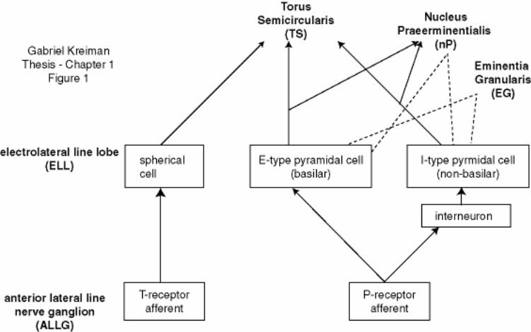
Figure 1-1: Schematic of the initial stages of the amplitude sensory pathway in
Eigenmannia ............................................................................................................. 26
Figure 1-2: Stimulus .................................................................................................... 26
Figure 1-3: Wiener-Kolmogorov filtering ................................................................... 27
Figure 1-4: Feature extraction...................................................................................... 27
Figure 1-5: Bursting neurons ....................................................................................... 28
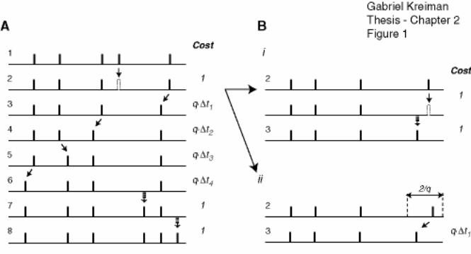
Figure 2-1: Computation of spike train distances........................................................ 74
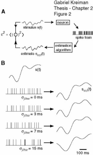
Figure 2-2: Quantification of stimulus encoding and of its robustness to spike time
jittering. 74
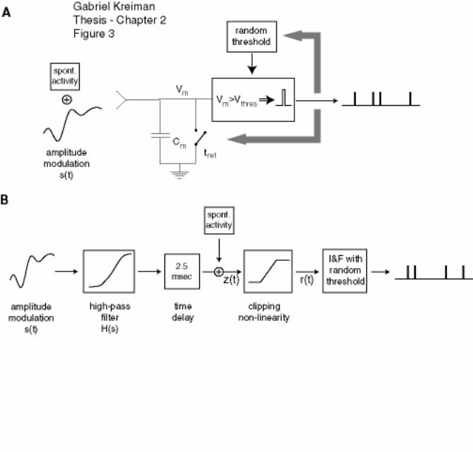
Figure 2-3: Comparison of P-receptor afferent spike trains to integrate-and-fire
models. 75
Figure 2-4: P-receptor afferent responses to RAMs exhibit a broad range of
variability. ................................................................................................................. 75
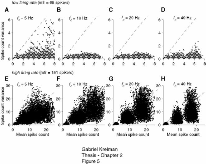
Figure 2-5: Scalloping of the variance vs. mean spike count relation is not a predictor
of spike timing variability. ........................................................................................ 76
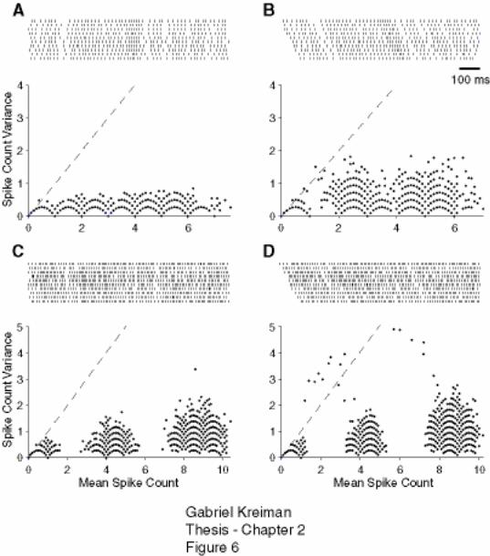
Figure 2-6: Scalloping of the variance vs. mean spike count relation measured across
trials is preserved even after large shifts in the timing of individual spike trains..... 77
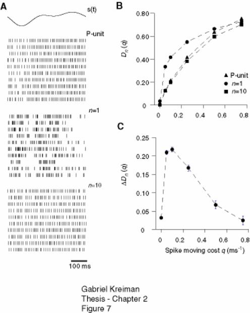
Figure 2-7: Spike train distances of P-receptor afferents match those of gamma
integrate-and-fire neurons with order n in the 3-10 range. ....................................... 77
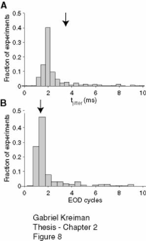
Figure 2-8: Distribution of mean spike time jitter in 69 P-receptor afferents
(corresponding to 508 different RAM stimulations)................................................. 78
Gabriel Kreiman Thesis xii
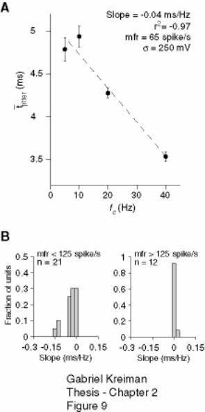
Figure 2-9: The timing jitter decreases with stimulus cut-off frequency at low but not
at high firing rates. .................................................................................................... 78
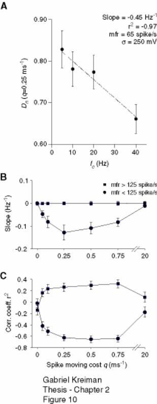
Figure 2-10: Increase in timing precision with stimulus cut-off frequency at low but not
at high firing rate is observed across a broad range of spike moving costs. ............. 79
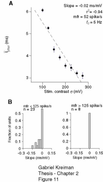
Figure 2-11: The timing jitter decreases with increasing stimulus contrast at low but not
at high firing rates. .................................................................................................... 79
Figure 2-12: Increase in timing precision as a function of stimulus contrast is observed
at low but not at high firing rates across a broad range of spike moving costs. ....... 79
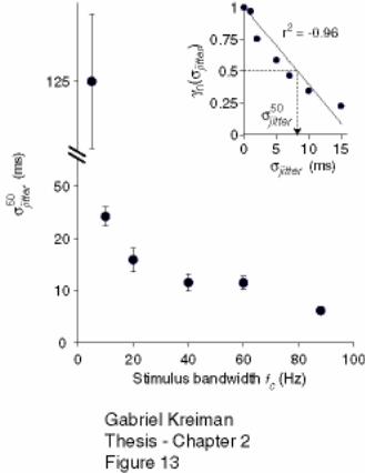
Figure 2-13: Robustness of RAM encoding decreases with stimulus bandwidth. ........ 80
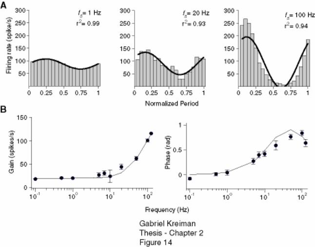
Figure 2-14: Fit of linear transfer function properties of a P-receptor afferent by a first
order high-pass filter. ................................................................................................ 80
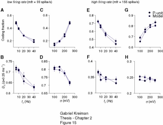
Figure 2-15: Comparison of spike train distances and stimulus encoding properties of
P-receptor afferents and model. ................................................................................ 81
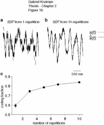
Figure 2-16: Stimulus reconstruction from the spike density function ......................... 81
Figure 2-17: Schematic of an oversampled Σ∆ converter ............................................. 82
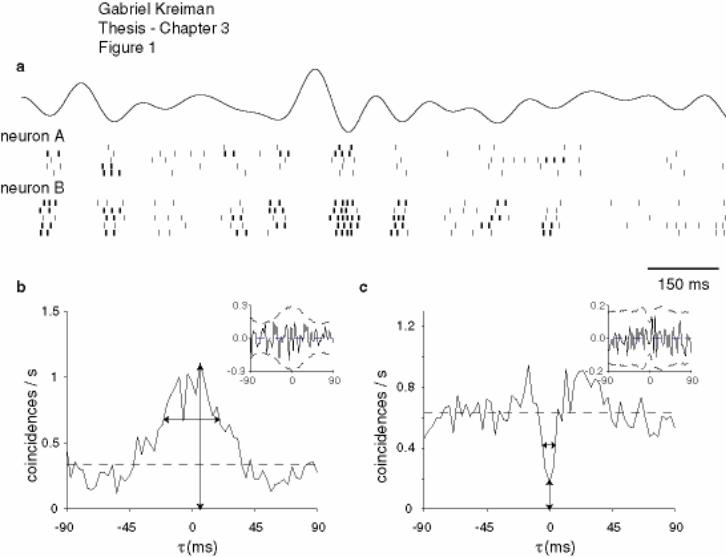
Figure 3-1 Correlated activity of simultaneously recorded pyramidal cells............. 130
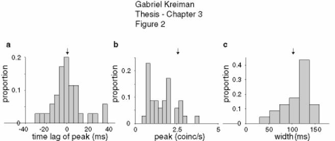
Figure 3-2 Properties of the cross-correlograms for pairs of units of the same type 131
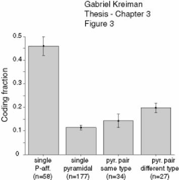
Figure 3-3 Summarized results of stimulus estimation ............................................ 131
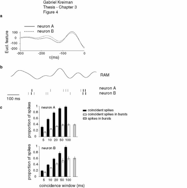
Figure 3-4 Euclidian features and coincident spikes ................................................ 131
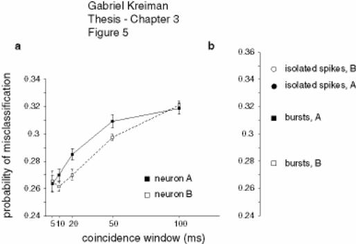
Figure 3-5 Feature extraction for pyramidal cell pairs ............................................. 132
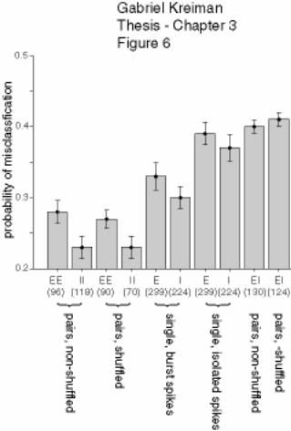
Figure 3-6 Summary diagram of feature extraction performance by ELL pyramidal
cells. 132
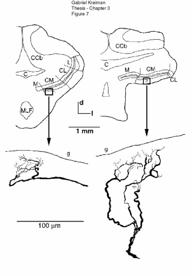
Figure 3-7 Terminal spread of P-receptor afferents ................................................. 133

Gabriel Kreiman Thesis xiii
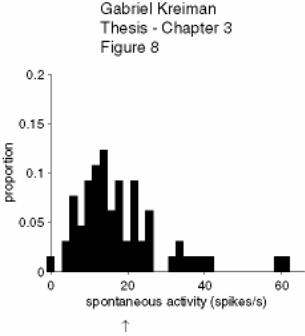
Figure 3-8: Spontaneous activity of pyramidal cells ................................................. 134
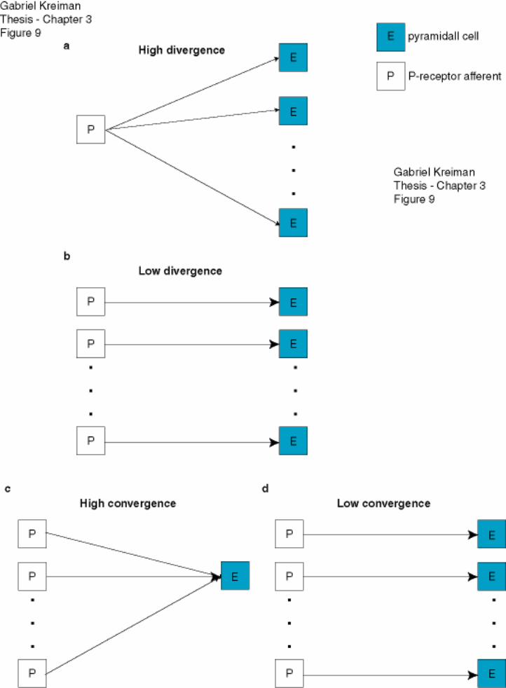
Figure 3-9: Schematic of different anatomical configurations for the P-receptor to
ELL projection ........................................................................................................ 134
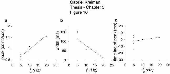
Figure 3-10: Change in correlogram properties with the stimulus bandwidth ............ 135
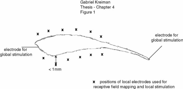
Figure 4-1: Schematic of stimulation procedure........................................................ 159
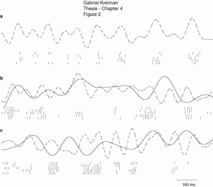
Figure 4-2: Pyramidal neuron activity, raster plot example ...................................... 159
Figure 4-3: Example of global versus local stimulation ............................................ 159
Figure 4-4: Pyramidal neuronal trial-to-trial firing variability .................................. 160
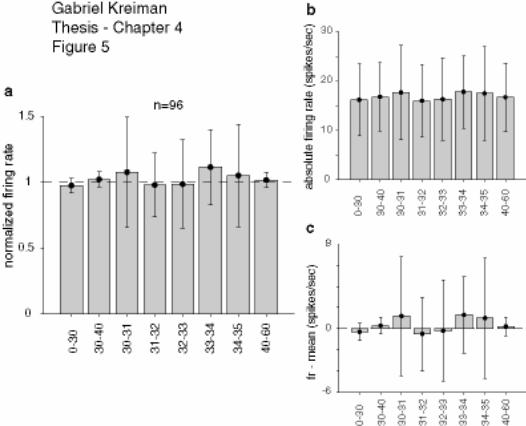
Figure 4-5: Changes in firing rate, summary............................................................. 160
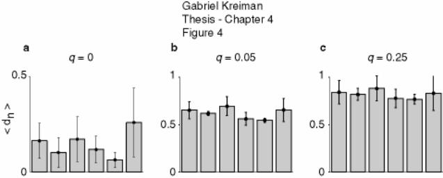
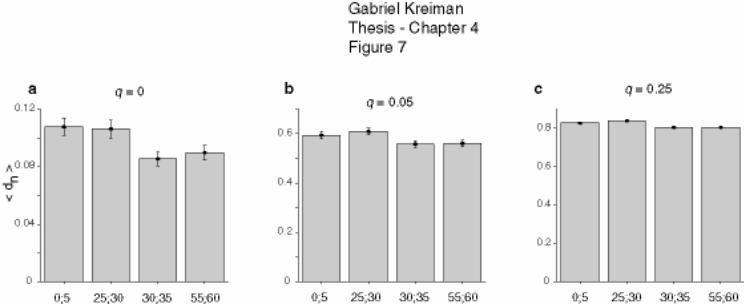
Figure 4-6: Changes in probability of misclassification, summary........................... 161
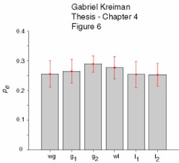
Figure 4-7: Changes in neuronal response variability, summary .............................. 161
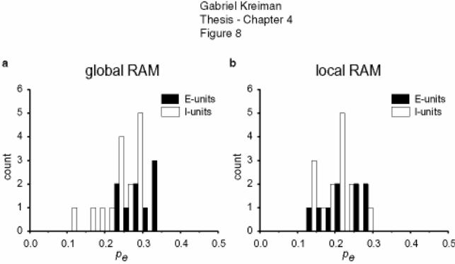
Figure 4-8: Comparison of E versus I pyramidal cells under different stimulation
conditions ................................................................................................................ 161

Gabriel Kreiman Thesis xiv
List of Tables
Table 2-1: Robustness to spike time jittering, and random spike additions or
deletions. 73
Gabriel Kreiman Thesis - Chapter 1 1
1 The investigation of neuronal codes
1.1 What is a neuronal code?
Signals from the environment are transduced by the senses into electrochemical
changes that can be interpreted by the brain. Neurons process the incoming information
and can direct the muscles to produce some output movement accordingly. The activity
of neurons in the brain must therefore represent somehow the input. The nature of this
representation is still unclear in most sensory systems and modalities and constitutes at
the time of writing this Thesis an extensively debated and fascinating problem that will
prove fundamental in trying to understand how the brain processes information.
An analogy may be useful. A photograph may be digitally stored in a computer. A
series of zeros and ones (in a binary computer) thus represents the given picture at a
given spatial and color resolution. This encoding is not unique (there are, for example,
different possible formats such as JPEG, GIF, TIFF and so on.) In the case of digital
pictures, we know perfectly well how to encode and decode the information so that given
a picture, we can convert it to, for example, a JPEG file and given a JPEG file, we can
display the picture in the computer. We can also predict how the series of zeros and ones
would change upon altering the image and how the picture would be distorted if we
corrupted the representation in the computer. This is not so trivial in the brain. The work

Gabriel Kreiman Thesis - Chapter 1 2
in the current Thesis is aimed towards understanding the representation of time-varying
signals by single neurons using the electric fish as an ideal model system to combine
neurophysiological exploration and computational analysis.
1.2 Organization of the Thesis1
This Thesis is subdivided into five separate but related Chapters. The current
Chapter describes some of the background and methodological procedures that are used
throughout the work. First, I will describe the experimental model that we have used in
our electrophysiological explorations: the Eigenmannia weakly electric fish. I will give a
brief overview of the history of some investigations about electric fish. I will describe
what is known about their Neuroanatomy, as well as their Neurophysiology as related to
our discussions in the current work. I will give an introduction to some of the theoretical
and empirical ideas and models that have been proposed for the mechanisms of
information encoding in the central nervous system. I will explain some of the
experimental and theoretical tools that are used in the subsequent Chapters including
Wiener-Kolmogorov stimulus reconstruction and feature extraction.
1 Part of the work described in the current Thesis has already been published in the form of a manuscript or is currently in press (Kreiman et al., 2000b, Krahe et al., 2002). Chapter 2 describes our results published in the Journal of Neurophysiology (Kreiman et al., 2000b) while Chapter 3 describes our results published in the Journal of Neuroscience. While part of the text is a repetition of the content of those manuscripts, there are several additional details, discussions, figures and comments that did not form part of the publications. The content of the other Chapters has not been published yet. Therefore, I hope the reader will find the current text interesting and worth reading even if he has already read the manuscripts. The converse is also true: other research projects that I worked on during my five years at Caltech are not covered in the current Thesis (see for example Kreiman et al., 2000a, Kreiman et al., 2000c, Kreiman et al., 2001). In particular, it is worth noting that the contents of this Thesis show no overlap with those reported in my other Thesis on the responses of individual neurons in the human brain (Kreiman et al., 2001).
Gabriel Kreiman Thesis - Chapter 1 3
In Chapter 2, I will describe our explorations of the robustness and variability of
the neural code by the primary amplitude-coding sensory afferents. We have applied a
novel spike metric developed by Victor and Purpura (Victor and Purpura, 1997) to
characterize the variability in neuronal recordings and used this measure to show that P-
receptor afferents can show reliable spiking responses with small time jitter on the order
of a few ms. This level of jitter depended on the temporal characteristics of the stimulus.
Furthermore, we quantitatively defined the robustness of the code to spike time jittering,
spike deletions and additions. We combined the data about the variability and robustness
to show that the degree of trial-to-trial variability occurs within a range that does not
significantly degrade the quality of information conveyed by P-units. Finally, we built a
simple model that incorporated the filtering properties of P-units and could account for
the encoding, variability and robustness of the experimentally recorded spike trains.
In Chapter 3, I will describe our study of the characterization of the stimulus
reconstruction and feature extraction by pairs of pyramidal cells recorded using two
electrodes. We explored whether highly correlated responses of nearby neurons within
topographic sensory maps are merely a sign of redundant information transmission or
whether they carry relevant information. For this purpose, we recorded simultaneously
from pairs of electrosensory pyramidal cells in a somatotopic map in the electrosensory
lateral line lobe of the weakly electric fish, Eigenmannia, while randomly modulating the
amplitude of a mimic of the animal's electric field. Previous work had shown that single
pyramidal cells encode the stimulus time course only poorly. Instead, they extract
upstrokes and downstrokes in stimulus amplitude by firing short bursts of spikes that
reliably indicate the presence of behaviorally relevant stimulus features. Extending these
Gabriel Kreiman Thesis - Chapter 1 4
approaches to pairs of pyramidal cells with overlapping receptive fields, we found that:
(1) pyramidal cell-pairs exhibit strong correlations on a time scale of several tens of
milliseconds, mainly due to time-locking of spikes to the stimulus and not to common
synaptic input. (2) This was corroborated by Neurobiotin-labeling of primary afferent
fibers, yielding an estimated divergence of one afferent fiber onto only 3-8 pyramidal
cells. (3) In a feature-extraction task, pyramidal cell-pairs perform significantly better
than single pyramidal cells. Thus, our results demonstrate that while the occurrence of
stimulus features can be reliably indicated by spike bursts of single pyramidal cells, this
reliability significantly increases by considering stimulus-induced coincident activity
across multiple neurons, i.e. by evaluating "distributed bursts" of spikes.
In Chapter 4, I will briefly discuss two other experiments that we carried out. The
first one involves our preliminary attempts to explore what I consider to be a very
interesting question. Attention has been shown to play a fundamental role in the
processing of sensory information, particularly in the visual system (see for example
(Fries et al., 2001, Resnik et al., 1997, Desimone and Duncan, 1995, Julesz, 1991,
Steinmetz et al., 2000, McAdams and Maunsell, 1999).) The Eigenmannia electric fish
constitute an ideal model for the study of how sensory information can be gated due to
attention and saliency. Furthermore, feedback from higher order brain structures has been
hypothesized to play a fundamental role in biasing the competition between different
stimuli and can be readily manipulated pharmacologically in the electric fish. I will
describe our first attempts to define attention and saliency within the electric modality
and our so far unsuccessful exploration of the neurophysiological changes that could
accompany the appearance of salient stimuli. The second experiment that I will describe

Gabriel Kreiman Thesis - Chapter 1 5
in this Chapter involves a detailed comparison of the responses of the two types of
pyramidal cells, the E and I cells, under global and local stimulation conditions. The
original report of Fabrizio Gabbiani and Walter Metzner showed that I cells perform
better at feature extraction than E cells (Metzner et al., 1998, see also our results in
Chapter 3). Our data show that this difference seems to be smaller for local stimulation.
Finally, in Chapter 5 I briefly summarize our observations and I discuss our
conclusions in the general context of other current investigations of the types of neuronal
codes used by the brain.
1.3 Brief history of inquires into neural coding
As in many other scientific fields, one of the main limitations is the kind of
experimental observations that can be acquired. The extracellular electrical spiking
activity of neurons constitutes one of the most readily accessible variables from an
experimental point of view. Thus, this has been and continues to be the most important
experimental variable used in the search for a correlation between neuronal activity and
behavior or perception.
The development of a method to detect and amplify small electrical signals was
provided in the beginning of the twentieth century with the invention of the vacuum tube.
Using these new instruments, Lucas at Cambridge University built new devices that
allowed recording signals of amplitude in the order of microvolts. Adrian and Hartline
laid the foundations of neuroelectrophysiology in the 1920s. One of the important
observations that Adrian made was that in response to a static stimulus the rate of spiking
Gabriel Kreiman Thesis - Chapter 1 6
increases as the stimulus becomes larger. This was done by increasing the load on a
stretch receptor. This has lead to the interpretation that the number of spikes in a fixed
time window after stimulus onset can represent the intensity or some other quality of the
stimulus. This hypothesis, typically called nowadays the "rate coding hypothesis", has
pervaded the history of neurophysiologic exploration ever since. Hartline independently
made similar observations studying the responses of single neurons in the compound eyes
of the horseshoe crab. Several decades later, Perkel and Bullock presented an overview of
different possible strategies for the encoding of information by neurons in different
systems (Perkel and Bullock, 1968).
The last decade of the last millennium saw a resurgence of interest in different
possibilities that individual neurons or groups of neurons may use to represent
information from the environment or to direct movements. While a large fraction of
neurophysiologists still utilize the spike count in relatively long windows to study the
neuronal activity, several papers have been reported that convey the picture that, at least
under certain specific conditions, neurons can show remarkable precision, that
coincidence detection can play a fundamental role and that synchronous activity could be
involved in encoding mechanisms. Furthermore, the study of time varying signals
showed that individual neurons could convey a large number of bits per second, in some
cases even close to the physical limits to information transmission.
At the time of writing this Thesis, several aspects of the encoding mechanism are
still under continuous and fascinating debate. The question of whether the relevant
variable is the spike count in long time windows of several hundred ms or the precise
timing of spikes at the ms level has been converted into a more precise and quantitative

Gabriel Kreiman Thesis - Chapter 1 7
formulation that centers around what are the relevant widths of the time windows. The
rate coding versus time coding debate are two extremes in a continuum and the exact
answer could depend on the type of stimuli (static versus time-varying) but also on the
precise parameters of stimulation. In addition to this question (but clearly related to it), a
pressing debate is centered on the issue of how ensembles of neurons encode information
and the role of synchrony and correlated activity. Technological advances have made it
possible to record the simultaneous activity of several neurons through tetrodes and
multiple electrode arrays over the last two decades, yielding new data to investigate this
problem. This will be discussed in Chapter 3.
1.4 Eigenmannia as a model
The Eigenmannia electric fish has proven to be a fascinating model to investigate
questions related to how neurons encode information. This is at least partly due to the
possibility of combining computational and electrophysiological approaches but also
because of the wealth of available information about the anatomy as well as behavior of
the fish. We know enough about the fish to be able to make progress without starting
from scratch and at the same time there is a sufficient number of open questions to make
research worthwhile.
There is a very long history of investigations concerning electric fish ranging
from their putative healing powers as ascribed by the Egyptians to the first

Gabriel Kreiman Thesis - Chapter 1 8
demonstrations of electrical conduction in biological tissue2. Two groups of tropical
freshwater fish, one South American and one African, send and receive weak electric
signals that are used in social communication and for electrolocation. Electric
communication is a highly evolved system with many functions that include sex and
species recognition, courtship behavior, mate assessment, territoriality and other forms of
spatial behavior, appeasement alarm and aggression. Six philogenetically diverse groups
of fishes evolved electric organs but only the South American Gymnotiformes and the
African Mormyriformes developed the use of these organs for communication. Electric
organ discharges (EOD) in these groups are characterized by a stereotyped waveform
fixed by the anatomy and physiology of the electric organ in the fish's tail. EODs do not
appear to be modulated under voluntary control. In addition to these discharges, the fish
can emit sequences of pulse discharges (SPIs) that make up the widely varying repertoire
of social signals. The fish that we have used as a model throughout this Thesis belong to
the Eigenmannia family. These weakly electric knife-fish can generate quasi-sinusoidal
continuous discharges by periodically discharging their electric organ at rates between
200 and 600 Hz (see Chapter 2).
2 The Egyptians and Greeks already knew about the shocking powers of some of the Nile fish and the electric ray. Galen turned to the use of electricity generated by fish for therapeutic purposes. He mostly recurred to the strong output of the electric rays for headaches, pain and even for epileptic seizures. This use of electricity generated by fish continued for several centuries afterwards and, given the difficulty of obtaining electric rays, stimulated the construction of "friction machines" to be able to generate electricity. Electrotherapy became extremely popular in the eighteenth century in Europe and North America. These observations lead to the idea that electricity may constitute the essential "fluid of the nerves". It was John Walsh who first demonstrated during the 1770s that electric fish can discharge electricity that could be transmitted through wires. He also studied the fine structure of the ray's electrical organs. The notion that the discharges originated in this specific organs showed that there was some form of insulation so that electricity could not disseminate into surrounding tissues, which was one of the key arguments against the notion of electrical fluids within nerves. The brilliant experiments of John Walsh paved the way to the notion of electrical activity in living animals as a major way of conveying signals. Skeptics, however, still argued that this was an extravagance of specialized fish that did not generalize to other animals like frogs or even humans. It was Luigi Galvani's revolutionary work that settled this argument at the end of the eighteenth century with his famous muscle nerve preparation in frogs (Galvani, 1953 (1791), Finger, 2000).
Gabriel Kreiman Thesis - Chapter 1 9
Arrays of receptors on the body surface monitor distortions of the amplitude and
phase of the electric field for electrolocation and communication purposes (for review see
(Heiligenberg, 1991)). The pattern of these distortions represents the electric image of
objects. The presence of an object in the water near the fish affects the amplitude and
phase of the signal. Although all ancestral forms of fish appear to have been
electroreceptive, this sensory modality was lost with the evolution of the teleost fishes.
This loss is as much a puzzle as its apparent reappearance in some groups of teleosts. The
original types of electroreceptors were ampullary organs and are most sensitive to low
frequency signals. These organs detect weak electric fields of geophysical, chemical or
biological origin and enable fish to orient and navigate in reference to large-scale fields in
oceans and river waters. In addition to these, Eigenmannia possess tuberous rectors that
are most sensitive in the range of the dominant spectral frequency of the animal's EODs.
These serve in electrolocation and communication. Electric fish have assumed a
dominant role in the nightly waters of the tropics by exploiting electrical cues. However,
EODs are limited to short distances.
Eigenmannia has two types of tuberous electroreceptors, P-type and T-type. The
somata of their primary afferents are located in the anterior lateral line nerve ganglion. P-
receptor afferents fire intermittently and increase their rate of firing with a rise in
stimulus amplitude. In contrast, T units fire one spike on each cycle of the stimulus and
the action potentials are phase locked with little jitter to the zero-crossings of the signal.
A schematic diagram illustrating the anatomy of the initial part of the electrosensory
system is shown in Figure 1-1. The information on amplitude and phase is relayed from
the electroreceptors embedded in the skin to the electrosensory lateral line lobe (ELL) in
Gabriel Kreiman Thesis - Chapter 1 10
the hindbrain, forming three somatotopic maps. A subset of primary sensory fibers, the P-
receptor afferents, encodes changes in the electric-field amplitude by firing in a
probabilistic manner (Scheich et al., 1973). P-receptor afferents synapse on E-type
pyramidal cells, which respond with excitation to increases in stimulus amplitude, and,
via interneurons, inhibit I-type pyramidal cells, which consequently fire spikes in
response to decreases in stimulus amplitude (Bastian, 1981, Maler et al., 1981). E- and I-
units are therefore analogous to ON and OFF cells in other sensory systems.
It is interesting to note that there is a strong parallel between the processing of
changes in the electric field, particularly for a specific behavior called the jamming
avoidance response (Heiligenberg and Partridge, 1981, Heiligenberg and Bastian, 1984,
Metzner and Juranek, 1997b), in the weakly electric fish and the neural algorithms for
sound localization in the owl's brain (Konishi, 1971, Konishi, 1991, Konishi, 1993,
Konishi, 1995).
1.5 Introduction to some of the methods
All the experimental work described in the current Thesis was carried out by
Rüdiger Krahe and Walter Metzner of the University of California at Riverside. Here I
will describe some of the general methodological procedures that are relevant for the
experiments and analyses detailed in the next Chapters. Specific details about the
methodology for each experiment are given within the context of Chapters 2, 3 and 4.
Gabriel Kreiman Thesis - Chapter 1 11
1.5.1 Stimulus
The electric field was established by a pair of carbon rod electrodes, one placed in
front or in the mouth of the animal and the other one behind the tail of the fish. Prior to
the experiment, the EOD frequency (fEOD) of the fish was determined. A sinusoidal
carrier signal with a frequency close to the fish's own EOD was generated by a function
generator (Exact 519, Hillsboro, OR) coupled to the electrodes. Electric field amplitude
modulations (AM) were synthesized and stored digitally (at either 2 kHz or 5 kHz) for
playback using commercial software (Signal Engineering Design, Belmong, MA and
LabView, National Instruments, Austin, TX). This allowed for repeated presentations of
the same stimulus (see Chapter 2). The AM and the carrier were gated by the same
trigger signal and were therefore phase locked to each other. The mean stimulus
amplitude, measured at the side fin perpendicular to the body axis, ranged from 1 to 5
mV/cm. To avoid under-driving the afferents, it was adjusted individually for each P-
receptor to stimulate it at 10 to 15 dB above threshold. The voltage generating the electric
stimulus, V(t), had a mean amplitude A0, and a carrier frequency fcarrier and was
modulated according to:
)2cos()](1[)( 0 tftsAtV carrierπ+= 1.1
A sample of the electric field presented to the fish including the carrier signal and the
amplitude modulation is illustrated in Figure 1-2a. The signal s(t) (Figure 1-2a and b)
constitutes the modulation of the electric field and the main matter of this Thesis will be
to try to understand how s(t) is represented by the activity of neurons in the fish nervous
system. For most of the experiments to be described here, s(t) was a random, zero-mean
signal with a flat power spectrum (white noise) up to a given cut-off frequency (fc) and
Gabriel Kreiman Thesis - Chapter 1 12
with a standard deviation σ (Figure 1-2c)3. A gaussian signal was generated in
MATLAB4. The signal was then low-pass filtered using a 4-pole Butterworth filter. The
stimulation caused a doubling of the carrier signal for s(t) = 1 V and a reduction to zero at
s(t) = -1 V. The values of fc and σ were varied from one repetition to another. The values
of fc used in the experiments were 5, 10, 20, 40 and 60 Hz. The contrast of the stimulus,
given by σ, was varied between 10 and 30% of the mean electric field amplitude (σ=100,
150, 200, 250, 275 and 300 mV). Consequently, amplitudes varied over a range of -20 to
-10 dB of the mean stimulus amplitude.
1.5.2 Electrophysiological recordings
Adult specimens of Eigenmannia, typically 15-20 cm long, were either bred and
raised in the laboratory or acquired from tropical fish wholesaler dealers (Bailey's, San
Diego, CA) under the commercial name of glass knife fish. Fish are maintained at 25 °C
in aquarium water. The water is adjusted for conductivity to a value of 10-20 kΩ/cm, pH
of 7 and 26-28 °C. After measuring the natural frequency of the fish electric organ
discharge, the animal is injected intramuscularly with Flaxedil (<5 µg/gm body weight;
gallamine thriethiodide, Sigma, St. Louis, MO) to paralyze the fish and also to block the
myogenic EOD. The fish is gently held on its side by a foam-lined clamp and ventilation
was provided by a stream of aerated water led into the animal's mouth through a glass
3 In some experiments a sinusoidal amplitude modulation was used to characterize the frequency responses function of P-receptor afferents (see Chapter 2). Also, in some experiments a band-pass random amplitude modulation signal was used. 4 The random number generator of MATLAB's 5.0 version allows to generate more than 1012 random independent values (see MATLAB reference manual and (Press et al., 1996)). The exact number of points in the signals that we used depends on the length of the signal and the digitization frequency but in no case was it larger than 106 (in most cases it was approximately 105). For each signal that was generated, a separate seed was used depending on the system time.
Gabriel Kreiman Thesis - Chapter 1 13
tube. Only the dorsal surface of its head protrudes above the water surface. A small
plexiglass rod was glued to the parietal bone under local anesthesia (2% lidocaine;
Western Medical Supplies, Arcadia, CA) to further stabilize the fish. The experimental
tank was situated on a vibration isolation table (Newport, Fountain Valley, CA). A
residual EOD-related signal (amplitude of 50 µV to 1 mV) locked to the spinal command
neurons could still be detected with a pair of wire electrodes placed next to the tail in
spite of the Flaxedil treatment. The curarization procedure, however, reduced the EOD
amplitude below the threshold level of the electroreceptors. .
To record the activity of single afferent units from electroreceptor organs located
on the animal's trunk, the posterior branch of the anterior lateral line nerve was exposed
just rostral to the operculum. This allowed for the extracellular recording of the activity
of single P-type afferents. Recordings were made with the use of 1M KCl-filled glass
electrodes (with 1kHz impedances around 40-60 MΩ) and an amplifier (WPI M707A,
Sarasota, FL). The indifferent electrode was a silver wire placed around the recording
electrode like a small ring. The afferent recordings were stored on tape (sampling rate 20
kHz, Vetter Instruments 300A, Redersburg, PA) and later A-D converted (sampling rate
10 kHz, Datawave, Denver, CO). Electroreceptor afferents were identified as P-type and
included in the study reported in Chapter 2 if:
1) the probability of firing per period of the EOC was <1 in the physiological
range of the electric field amplitude
2) the spontaneous activity was irregular (as opposed to bursting, characteristic of
T-type units).
Gabriel Kreiman Thesis - Chapter 1 14
3) the units phase-locked with large jitter (as opposed to small jitter for the T-type
units)
Animal handling and all surgical procedures were in accordance with NIH
guidelines and were approved by the local Institutional Animal Care and Use Committee
1.5.3 Stimulus reconstruction
Here I briefly review one of the main analytical tools that we have used
throughout this Thesis, namely, the linear reconstruction of amplitude modulations from
a spike train. This is a particular case derived from the general study of signal processing
theory where an attempt is made to estimate a particular signal from observations or
experimental measurements that can be subject to noise (Poor, 1994, Oppenheim et al.,
1997) and also draws extensively from the principles of information theory developed by
Shanon (Shannon and Weaver, 1949, Rieke et al., 1997). The quantitative exploration of
the amount of information conveyed by a spike train about a time-varying stimulus was
introduced into Neuroscience by Bill Bialek (Bialek et al., 1991) and has been applied in
several different systems including the fly visual motion system, the electric fish, the
retina and the cricket cercal system (Wessel et al., 1996, Theunissen et al., 1996,
Gabbiani and Koch, 1996, Warland et al., 1997, Stanley et al., 1999, Dan et al., 1998).
Excellent overviews of these analytical techniques have been written by Rieke et al
(Rieke et al., 1997) and Fabrizio Gabbiani (Gabbiani and Koch, 1998).
Let s(t) represent the zero-mean stimulus (in our case this will correspond to the
random amplitude modulation of the electric field and has been described in more detail
in Section 1.5.1). Let us represent the spike train by:
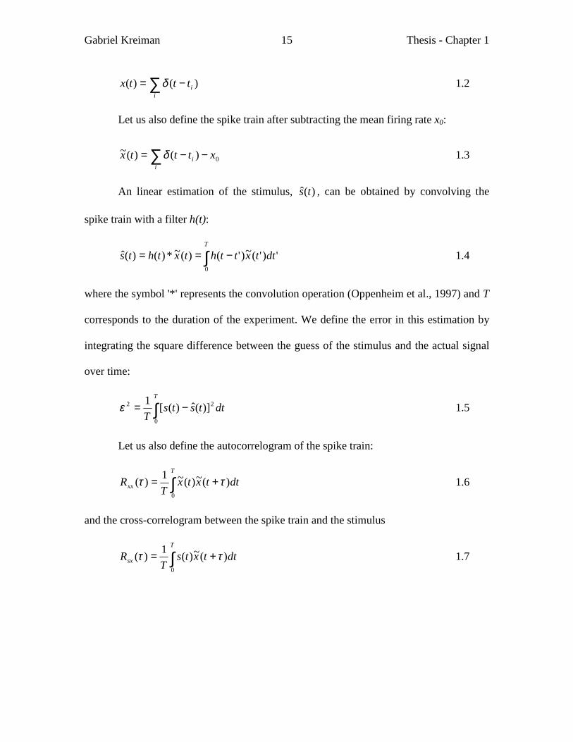
Gabriel Kreiman Thesis - Chapter 1 15
)()( ∑ −=i
itttx δ 1.2
Let us also define the spike train after subtracting the mean firing rate x0:
∑ −−=i
i xtttx 0)()(~ δ 1.3
An linear estimation of the stimulus, )(ˆ ts , can be obtained by convolving the
spike train with a filter h(t):
∫ −==T
dttxtthtxthts0
')'(~)'()(~*)()(ˆ 1.4
where the symbol '*' represents the convolution operation (Oppenheim et al., 1997) and T
corresponds to the duration of the experiment. We define the error in this estimation by
integrating the square difference between the guess of the stimulus and the actual signal
over time:
∫ −=T
dttstsT 0
22 )](ˆ)([1ε 1.5
Let us also define the autocorrelogram of the spike train:
∫ +=T
xx dttxtxT
R0
)(~)(~1)( ττ 1.6
and the cross-correlogram between the spike train and the stimulus
∫ +=T
sx dttxtsT
R0
)(~)(1)( ττ 1.7

Gabriel Kreiman Thesis - Chapter 1 16
After Fourier transformation, these are known in the frequency domain as the
power spectrum of the spike train, )(ωxxS , and the cross-spectrum between stimulus and
spike train, )(ωsxS (with ω=2πf) 5.
The error in the estimation will generally depend on the choice of the filter h(t).
The Wiener-Kolmogorov filter minimizes the square error and can be easily obtained
from the orthogonality condition (Poor, 1994, Gabbiani and Koch, 1996, Gabbiani,
1996). The shape of this filter is illustrated in one case of reconstruction in Figure 1-3a.
The resulting expressions for the filter in the time and frequency domains are:
∫−
−−=
c
c
f
f
ift
xx
sx dfefSfSth π2
)()(
)( 1.8
)()(
)(fSfS
fHxx
sx −= 1.9
Let us also define the noise as a function of time given by the difference between
the stimulus and its estimate:
)()(ˆ)( tststn −= 1.10
Then the square error can be expressed as: ∫>==< ωωπ
ε dStn nn )(21|)(| 22 where "|x|"
denotes the absolute value of variable x, the "<x>"
indicates time average and Snn is the power spectrum of the noise. From the definition of
the noise it is evident that: )()(|)(|
)()(2
ωω
ωωω stimxx
sxstimnn S
SS
SS ≤−= where Sstim(ω) is the
5 ∫= πττ 2/)()( if
xxxx eRfS and ∫= πττ 2/)()( ifsxsx eRfS

Gabriel Kreiman Thesis - Chapter 1 17
power spectrum of the stimulus. Therefore, if we define the signal-to-noise ratio (SNR)6
as:
)()(
)(ωω
ωnn
stim
SS
SNR = 1.11
The SNR as a function of frequency is shown in Figure 1-3b and shows for the
current example that there is an enhanced signal reconstructed above the noise (SNR>1)
up to the stimulus bandwidth. We may rewrite the expression for the mean square error
as:
ωωω
πε
ω
ω
dSNRSc
c
stim∫−
=)()(
212 1.12
This allows us to evaluate the quality of the reconstruction in specific frequency
bands (see for example Chapter 4). If the spike train is completely uncorrelated with the
signal, then SNR(ω)=1 for all frequencies within the stimulus band. In this case, the mean
square error is the integral of the power spectrum of the stimulus which is the variance of
the stimulus, σ2.
1)( =ωSNR cωω ≤∀ || ⇒ 22 )( σωωε ∫ == dSstim 1.13
Since the magnitude of ε2 can vary from one system to another and also from one
experiment to another, it is convenient to express the accuracy of the estimation in a
dimensionless variable, the coding fraction, which we will define as:
σεγ −=1 1.14
6 Note that SNR(ω)≥1
Gabriel Kreiman Thesis - Chapter 1 18
where σ is the standard deviation of the stimulus. It follows from equations 1.12-13 that
the error is bounded by σ and therefore 0 ≤ γ ≤ 1. An example of a RAM stimulus and its
estimation is shown in Figure 1-3c-e. Although, the estimated stimulus clearly does not
perfectly match the original signal, the similarity between the two signals is quite striking
particularly if we consider that this is obtained from linear reconstruction using a single
spike train.
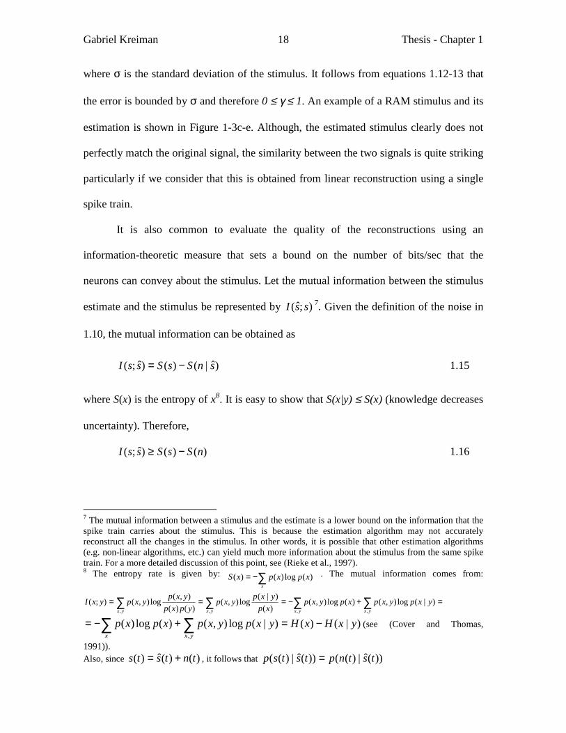
It is also common to evaluate the quality of the reconstructions using an
information-theoretic measure that sets a bound on the number of bits/sec that the
neurons can convey about the stimulus. Let the mutual information between the stimulus
estimate and the stimulus be represented by );ˆ( ssI 7. Given the definition of the noise in
1.10, the mutual information can be obtained as
)ˆ|()()ˆ;( snSsSssI −= 1.15
where S(x) is the entropy of x8. It is easy to show that S(x|y) ≤ S(x) (knowledge decreases
uncertainty). Therefore,
)()()ˆ;( nSsSssI −≥ 1.16
7 The mutual information between a stimulus and the estimate is a lower bound on the information that the spike train carries about the stimulus. This is because the estimation algorithm may not accurately reconstruct all the changes in the stimulus. In other words, it is possible that other estimation algorithms (e.g. non-linear algorithms, etc.) can yield much more information about the stimulus from the same spike train. For a more detailed discussion of this point, see (Rieke et al., 1997). 8 The entropy rate is given by: ∑−=
xxpxpxS )(log)()( . The mutual information comes from:
∑ ∑ ∑ ∑ =+−===yx yx yx yx
yxpyxpxpyxpxp
yxpyxpypxp
yxpyxpyxI, , , ,
)|(log),()(log),()(
)|(log),()()(
),(log),();(
)|()()|(log),()(log)(,
yxHxHyxpyxpxpxpx yx
∑ ∑ −=+−= (see (Cover and Thomas,
1991)). Also, since )()(ˆ)( tntsts += , it follows that ))(ˆ|)(())(ˆ|)(( tstnptstsp =

Gabriel Kreiman Thesis - Chapter 1 19
It can be shown that the entropy rate of a stationary process is always smaller than the
entropy rate of the corresponding stationary gaussian process (having the same
covariance as n) (Cover and Thomas, 1991): )()( nSnS G ≥ . Therefore,
LBG InSsSssI ≡−≥ )()()ˆ;( 1.17
A lower bound on the mutual information conveyed by )(ˆ ts about the stimulus, ILB, is
given by:
ωωπ
dSNRIc
c
w
wLB ∫
−
= )](log[)2log(4
1 1.18
(in bits per second.) It is clear from Equation 1.13 that no information is conveyed within
the frequency bands in which SNR(ω)=1. It is of interest to compare this lower bound
with the absolute lower bound or epsilon entropy that can be estimated for a bandwidth
limited white noise stimulus by:
−
=σε
ε log)2log(
cfI 1.19
and can be shown to be smaller or equal to ILB (Gabbiani, 1996). While there is in general
a monotonic relation between the coding fraction and the information rate, this is not
necessarily a linear one. A direct comparison of the two measures of stimulus
reconstruction can be found in (Gabbiani and Koch, 1996, Gabbiani, 1996, Wessel et al.,
1996). Throughout this Thesis, I will use the coding fraction to assess the quality of the
reconstructed stimulus. This is a dimensionless measure that can be readily interpreted
and compared in different systems.
Gabriel Kreiman Thesis - Chapter 1 20
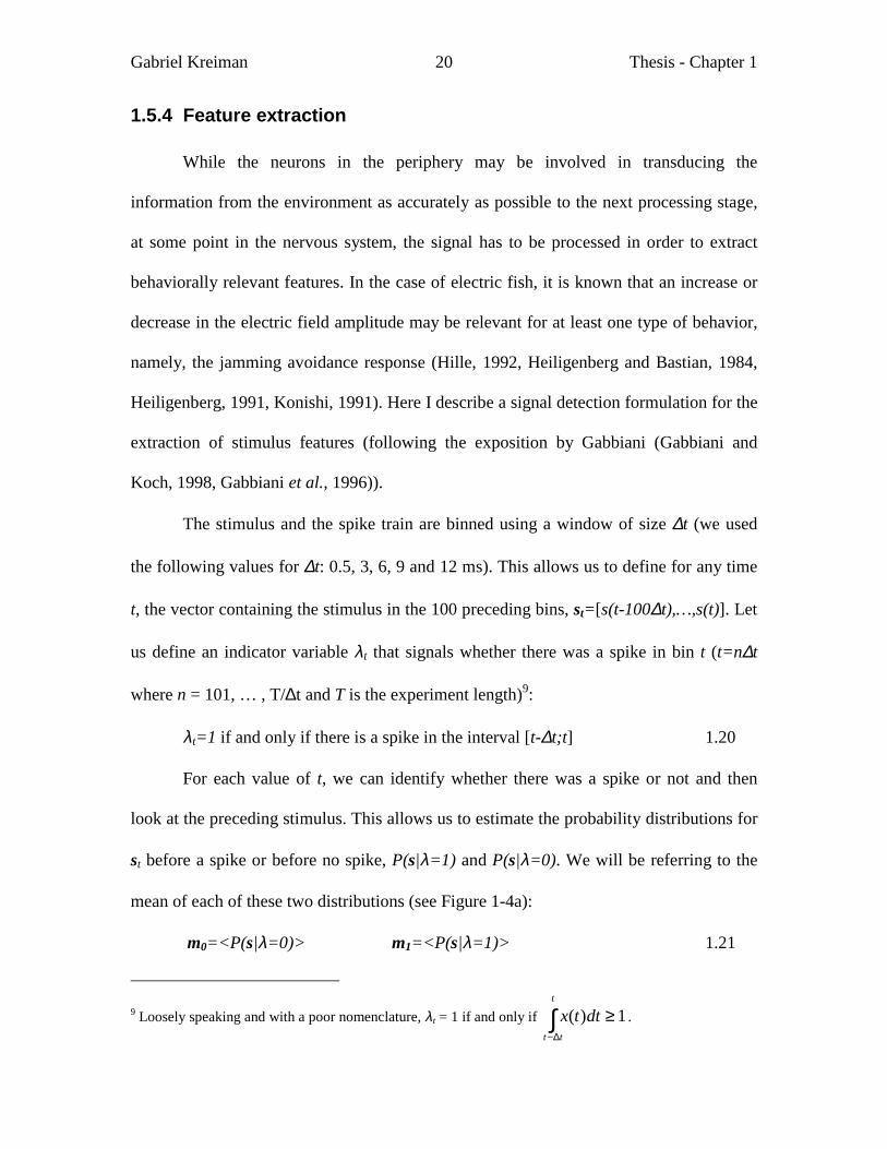
1.5.4 Feature extraction
While the neurons in the periphery may be involved in transducing the
information from the environment as accurately as possible to the next processing stage,
at some point in the nervous system, the signal has to be processed in order to extract
behaviorally relevant features. In the case of electric fish, it is known that an increase or
decrease in the electric field amplitude may be relevant for at least one type of behavior,
namely, the jamming avoidance response (Hille, 1992, Heiligenberg and Bastian, 1984,
Heiligenberg, 1991, Konishi, 1991). Here I describe a signal detection formulation for the
extraction of stimulus features (following the exposition by Gabbiani (Gabbiani and
Koch, 1998, Gabbiani et al., 1996)).
The stimulus and the spike train are binned using a window of size ∆t (we used
the following values for ∆t: 0.5, 3, 6, 9 and 12 ms). This allows us to define for any time
t, the vector containing the stimulus in the 100 preceding bins, st=[s(t-100∆t),…,s(t)]. Let
us define an indicator variable λt that signals whether there was a spike in bin t (t=n∆t
where n = 101, … , T/∆t and T is the experiment length)9:
λt=1 if and only if there is a spike in the interval [t-∆t;t] 1.20
For each value of t, we can identify whether there was a spike or not and then
look at the preceding stimulus. This allows us to estimate the probability distributions for
st before a spike or before no spike, P(s|λ=1) and P(s|λ=0). We will be referring to the
mean of each of these two distributions (see Figure 1-4a):
m0=<P(s|λ=0)> m1=<P(s|λ=1)> 1.21
9 Loosely speaking and with a poor nomenclature, λt = 1 if and only if ∫∆−
≥t
tt
dttx 1)( .
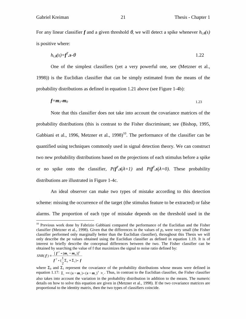
Gabriel Kreiman Thesis - Chapter 1 21
For any linear classifier f and a given threshold θ, we will detect a spike whenever ht,θ(s)
is positive where:
ht,θ(s)=fT.s-θ 1.22
One of the simplest classifiers (yet a very powerful one, see (Metzner et al.,
1998)) is the Euclidian classifier that can be simply estimated from the means of the
probability distributions as defined in equation 1.21 above (see Figure 1-4b):
f=m1-m0 1.23
Note that this classifier does not take into account the covariance matrices of the
probability distributions (this is contrast to the Fisher discriminant; see (Bishop, 1995,
Gabbiani et al., 1996, Metzner et al., 1998)10. The performance of the classifier can be
quantified using techniques commonly used in signal detection theory. We can construct
two new probability distributions based on the projections of each stimulus before a spike
or no spike onto the classifier, P(fT.s|λ=1) and P(fT.s|λ=0). These probability
distributions are illustrated in Figure 1-4c.
An ideal observer can make two types of mistake according to this detection
scheme: missing the occurrence of the target (the stimulus feature to be extracted) or false
alarms. The proportion of each type of mistake depends on the threshold used in the 10 Previous work done by Fabrizio Gabbiani compared the performance of the Euclidian and the Fisher classifier (Metzner et al., 1998). Given that the differences in the values of pe were very small (the Fisher classifier performed only marginally better than the Euclidian classifier), throughout this Thesis we will only describe the pe values obtained using the Euclidian classifier as defined in equation 1.19. It is of interest to briefly describe the conceptual differences between the two. The Fisher classifier can be obtained by searching the value of f that maximizes the signal to noise ratio defined by:
ff
mmff••
•
Σ+Σ
−=
)21(
)]([)(
10
201
T
T
SNR
where Σ0 and Σ1 represent the covariance of the probability distributions whose means were defined in equation 1.17:
iT
iii >−−=<Σ • )()( msms . Thus, in contrast to the Euclidian classifier, the Fisher classifier also takes into account the variation in the probability distribution in addition to the means. The numeric details on how to solve this equation are given in (Metzner et al., 1998). If the two covariance matrices are proportional to the identity matrix, then the two types of classifiers coincide.
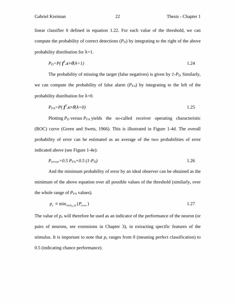
Gabriel Kreiman Thesis - Chapter 1 22
linear classifier h defined in equation 1.22. For each value of the threshold, we can
compute the probability of correct detections (PD) by integrating to the right of the above
probability distribution for λ=1.
PD=P( fT.s>θ|λ=1) 1.24
The probability of missing the target (false negatives) is given by 1-PD. Similarly,
we can compute the probability of false alarm (PFA) by integrating to the left of the
probability distribution for λ=0.
PFA=P( fT.s>θ|λ=0) 1.25
Plotting PD versus PFA yields the so-called receiver operating characteristic
(ROC) curve (Green and Swets, 1966). This is illustrated in Figure 1-4d. The overall
probability of error can be estimated as an average of the two probabilities of error
indicated above (see Figure 1-4e):
Perrror=0.5 PFA+0.5 (1-PD) 1.26
And the minimum probability of error by an ideal observer can be obtained as the
minimum of the above equation over all possible values of the threshold (similarly, over
the whole range of PFA values).
)(min 10 errorPe PpFA ≤≤= 1.27
The value of pe will therefore be used as an indicator of the performance of the neuron (or
pairs of neurons, see extensions in Chapter 3), in extracting specific features of the
stimulus. It is important to note that pe ranges from 0 (meaning perfect classification) to
0.5 (indicating chance performance).
Gabriel Kreiman Thesis - Chapter 1 23
1.5.5 Bursting
In spite of the laborious effort that involves recording the spiking activity of
individual neurons, it is important to keep in mind that the message conveyed by many
action potentials does not reach the post-synaptic neuron. This is due to several factors
that include failure in action potential propagation, stochastic nature of neurotransmitter
release given an action potential and variability in post-synaptic response. One important
determinant of the efficacy of action potentials in being conveyed seems to be the
occurrence of several spikes within a short time interval. Many neurons seem to show
this bursting type of behavior (see (Steriade, 2001, Sherman, 2001, Guido et al., 1995,
Larkum et al., 1999, Bair et al., 1994, Lisman, 1997, Metzner et al., 1998, Bastian and
Nguyenkim, 2001, Martinez-Conde et al., 2000, Reinagel et al., 1999) and Figure 1-5).
We separately considered the performance of isolated spikes and spike bursts in the
feature extraction task outlined in the previous Section. The maximum interspike interval
that defined spikes belonging to a burst was taken from the first inflexion of the
interspike interval distribution (see Figure 1-5)11. As reported previously (Gabbiani et al.,
1996, Metzner et al., 1998), we observed that there was a strong enhancement in feature
extraction (both for I and E type pyramidal cells) when comparing spikes within bursts to
all spikes or isolated spikes. The results are described in Chapter 3.
11 We also compared this method of discriminating bursts with the direct comparison with a Poisson process as described by (Abeles, 1982, Bastian and Nguyenkim, 2001). The autocorrelogram of a Poisson process is flat and it is easy to compute confidence intervals to assess the statistical significance of departures from this null hypothesis. Both procedures gave similar results.
Gabriel Kreiman Thesis - Chapter 1 24
1.6 What would it mean to understand the neuronal code?
I define here two simple conditions that should be met if we wish to imply that we
understand the neuronal representation for a particular model by analogy with the
encoding of images in computers that we have just briefly described. Given the neuronal
response r we should be able to accurately estimate which stimulus s the system was
subject to. Conversely, given the stimulus, we should be able to predict the neuronal
response. This also implies that we would be able to predict what kind of changes in r
could be expected by specific alterations in s. We can go one step further; if the neuronal
response r indeed represents in a non-redundant way the information about s, altering r
should lead to changes in the system's internal representation of s and then potentially in
its behavior.
While it may seem easy to write these short lines in a piece of paper, empirically
assessing this correlation between the neuronal response and the stimulus can be quite
challenging. It should be noted that the neuronal response r in the previous paragraph
does not necessarily mean a single unit response. Registering the activity of large
numbers of individual neurons in a network is not an easy task, though. In other cases,
the stimulus set that is presented to a neuron could only represent a very small subset of
the possible set of stimuli the animal can experience. Thus, models may only be based on
a limited amount of information about the neuronal response. At least partly for this
reason, many models have been built that can account for available data but have a very
reduced power of extrapolation. Finally, proving in a convincing that altering the

Gabriel Kreiman Thesis - Chapter 1 25
neuronal response leads to a change in the animal's interpretation of the stimulus can also
be quite complicated from an experimental point of view.
Here we explore the first two stages of processing of information about a time-
continuous varying signal. We will argue that we have a relatively good understanding by
now of the first stage of transducing the stimulus from the environment into the spike
train of the sensory afferents. The stimulus can be quite accurately estimated given the
spike train and we have built a model that can predict the encoding, variability and
robustness of the neuronal responses. We also venture some conjectures about how small
groups of neurons can precisely transmit the information from the environment to the
next processing stage. At the next stage of processing, the detailed encoding of
information at the level of the primary sensory neurons gives rise to the possibility of
extracting behaviorally relevant features about the stimulus. More work will be required
to understand the biophysical mechanisms by which this feature extraction process can
take place. Eigenmannia offers a fascinating model for the detailed study of these
questions.
Gabriel Kreiman Thesis - Chapter 1 26
1.7 Figure legends
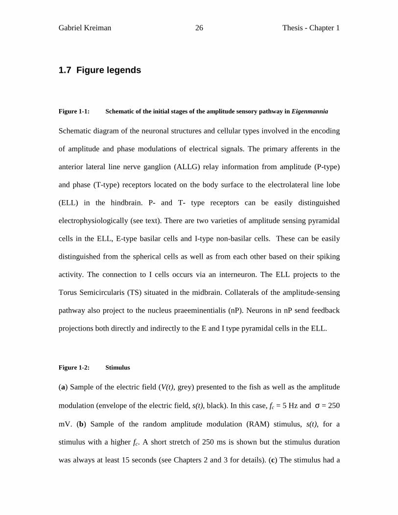
Figure 1-1: Schematic of the initial stages of the amplitude sensory pathway in Eigenmannia
Schematic diagram of the neuronal structures and cellular types involved in the encoding
of amplitude and phase modulations of electrical signals. The primary afferents in the
anterior lateral line nerve ganglion (ALLG) relay information from amplitude (P-type)
and phase (T-type) receptors located on the body surface to the electrolateral line lobe
(ELL) in the hindbrain. P- and T- type receptors can be easily distinguished
electrophysiologically (see text). There are two varieties of amplitude sensing pyramidal
cells in the ELL, E-type basilar cells and I-type non-basilar cells. These can be easily
distinguished from the spherical cells as well as from each other based on their spiking
activity. The connection to I cells occurs via an interneuron. The ELL projects to the
Torus Semicircularis (TS) situated in the midbrain. Collaterals of the amplitude-sensing
pathway also project to the nucleus praeeminentialis (nP). Neurons in nP send feedback
projections both directly and indirectly to the E and I type pyramidal cells in the ELL.
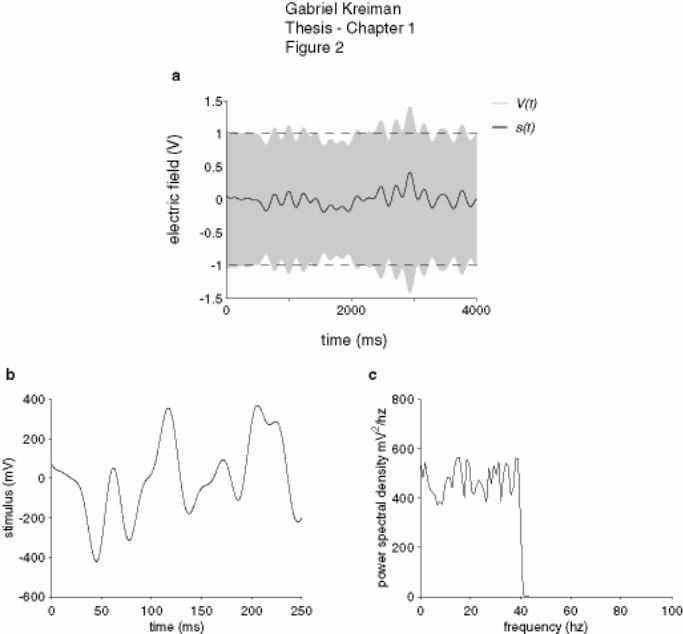
Figure 1-2: Stimulus
(a) Sample of the electric field (V(t), grey) presented to the fish as well as the amplitude
modulation (envelope of the electric field, s(t), black). In this case, fc = 5 Hz and σ = 250
mV. (b) Sample of the random amplitude modulation (RAM) stimulus, s(t), for a
stimulus with a higher fc. A short stretch of 250 ms is shown but the stimulus duration
was always at least 15 seconds (see Chapters 2 and 3 for details). (c) The stimulus had a
Gabriel Kreiman Thesis - Chapter 1 27
flat power spectrum up to a cut-off frequency fc (in this case fc = 40 Hz). The signal was
generated by using a 4-pole Butterworth filter (Oppenheim et al., 1997). The standard
deviation of the zero-mean stimulus depicted in this case was 200 mV.
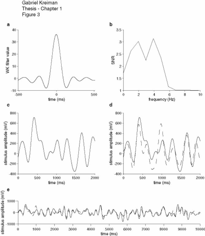
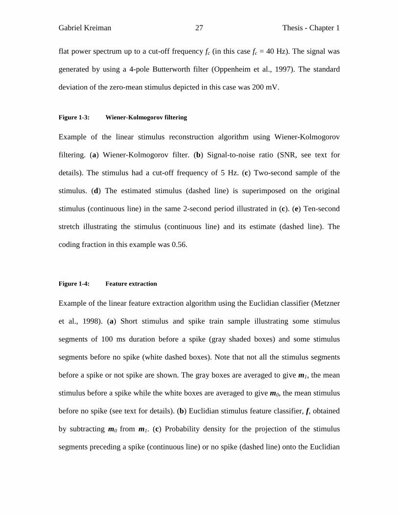
Figure 1-3: Wiener-Kolmogorov filtering
Example of the linear stimulus reconstruction algorithm using Wiener-Kolmogorov
filtering. (a) Wiener-Kolmogorov filter. (b) Signal-to-noise ratio (SNR, see text for
details). The stimulus had a cut-off frequency of 5 Hz. (c) Two-second sample of the
stimulus. (d) The estimated stimulus (dashed line) is superimposed on the original
stimulus (continuous line) in the same 2-second period illustrated in (c). (e) Ten-second
stretch illustrating the stimulus (continuous line) and its estimate (dashed line). The
coding fraction in this example was 0.56.
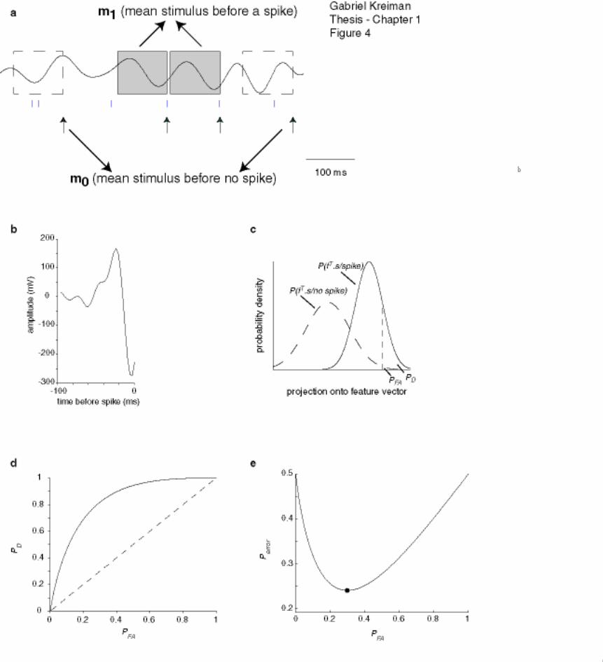
Figure 1-4: Feature extraction
Example of the linear feature extraction algorithm using the Euclidian classifier (Metzner
et al., 1998). (a) Short stimulus and spike train sample illustrating some stimulus
segments of 100 ms duration before a spike (gray shaded boxes) and some stimulus
segments before no spike (white dashed boxes). Note that not all the stimulus segments
before a spike or not spike are shown. The gray boxes are averaged to give m1, the mean
stimulus before a spike while the white boxes are averaged to give m0, the mean stimulus
before no spike (see text for details). (b) Euclidian stimulus feature classifier, f, obtained
by subtracting m0 from m1. (c) Probability density for the projection of the stimulus
segments preceding a spike (continuous line) or no spike (dashed line) onto the Euclidian
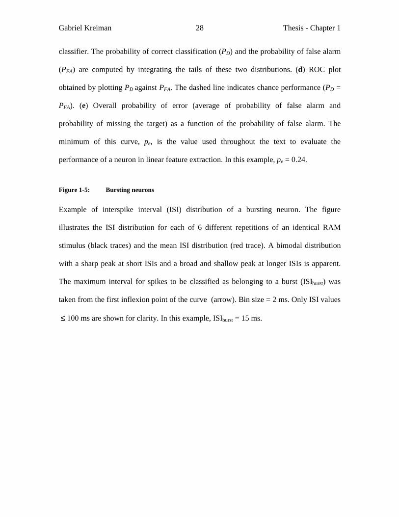
Gabriel Kreiman Thesis - Chapter 1 28
classifier. The probability of correct classification (PD) and the probability of false alarm
(PFA) are computed by integrating the tails of these two distributions. (d) ROC plot
obtained by plotting PD against PFA. The dashed line indicates chance performance (PD =
PFA). (e) Overall probability of error (average of probability of false alarm and
probability of missing the target) as a function of the probability of false alarm. The
minimum of this curve, pe, is the value used throughout the text to evaluate the
performance of a neuron in linear feature extraction. In this example, pe = 0.24.
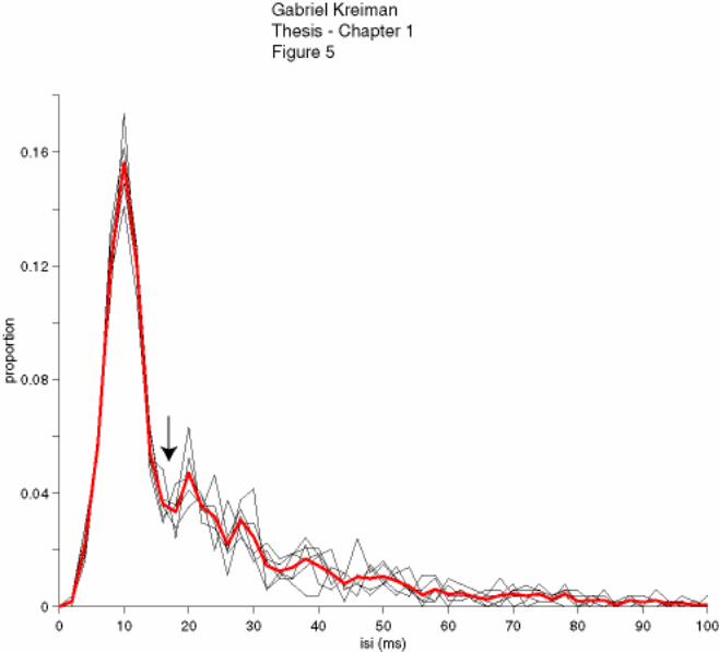
Figure 1-5: Bursting neurons
Example of interspike interval (ISI) distribution of a bursting neuron. The figure
illustrates the ISI distribution for each of 6 different repetitions of an identical RAM
stimulus (black traces) and the mean ISI distribution (red trace). A bimodal distribution
with a sharp peak at short ISIs and a broad and shallow peak at longer ISIs is apparent.
The maximum interval for spikes to be classified as belonging to a burst (ISIburst) was
taken from the first inflexion point of the curve (arrow). Bin size = 2 ms. Only ISI values
≤ 100 ms are shown for clarity. In this example, ISIburst = 15 ms.

Gabriel Kreiman Thesis - Chapter 2
34
2 Robustness, Variability and Modeling of P-receptor
afferents spike trains
2.1 Overview
We investigated the variability of P-receptor afferent spike trains in the weakly
electric fish, Eigenmannia, to repeated presentations of random electric field amplitude
modulations (RAMs) and quantified its impact on the encoding of time-varying stimuli.
A new measure of spike timing jitter was developed using the notion of spike train
distances recently introduced by Victor and Purpura (Victor and Purpura, 1996, Victor
and Purpura, 1997). This measure of variability is widely applicable to neuronal
responses, irrespective of the type of stimuli used (deterministic vs. random) or the
reliability of the recorded spike trains. In our data, the mean spike count and its variance
measured in short time windows were poorly correlated with the reliability of P-receptor
afferent spike trains, implying that such measures provide unreliable indices of trial-to-
trial variability. P-receptor afferent spike trains were considerably less variable than those
of Poisson model neurons. The average timing jitter of spikes lay within 1-2 cycles of the
electric organ discharge (EOD). At low, but not at high firing rates, the timing jitter was
dependent on the cut-off frequency of the stimulus and, to a lesser extent, on its contrast.
When spikes were artificially manipulated to increase jitter, information conveyed by P-
receptor afferents was degraded only for average jitters considerably larger than those
Gabriel Kreiman Thesis - Chapter 2
35
observed experimentally. This suggests that the intrinsic variability of single spike trains
lies outside of the range where it might degrade the information conveyed, yet still allows
for improvement in coding by averaging across multiple afferent fibers. Our results were
summarized in a phenomenological model of P-receptor afferents, incorporating both
their linear transfer properties and the variability of their spike trains. This model
complements an earlier one proposed by Nelson et al. (Nelson et al., 1997) for P-receptor
afferents of Apteronotus. Because of their relatively high precision with respect to the
EOD cycle frequency, P-receptor afferent spike trains possess the temporal resolution
necessary to support coincidence detection operations at the next stage in the amplitude-
coding pathway. The results described in the current Chapter were already reported
previously (Kreiman et al., 2000b).
2.2 Introduction
Variability has long attracted neurophysiologists as a tool to investigate the
biophysical mechanisms of sensory processing, the integrative properties of nerve cells
and the encoding schemes used in various parts of the nervous system (Baylor et al.,
1979, Hecht et al., 1942, Shadlen et al., 1996, Softky and Koch, 1993). Until recently,
most work has focused on characterizing the response variability of nerve cells to static
stimuli, in part because simple measures such as the variance of the number of spikes
recorded in long time windows provide universal and effective ways to quantify
variability under such conditions (Parker and Newsome, 1998).
Gabriel Kreiman Thesis - Chapter 2
36
Most biologically relevant stimuli, however, are not static. Therefore, more
recently investigators have started to characterize the trial-to-trial variability of responses
to time-varying, dynamic stimuli in vivo and in vitro (Bair and Koch, 1996, Berry et al.,
1997, Mainen and Sejnowski, 1995, Mechler et al., 1998, Stevens and Zador, 1998, van
Steveninck et al., 1997, Warzecha et al., 1998, Reich et al., 1997). When temporal
variations are sufficiently strong to induce locking of spikes to stimulus transients,
measures such as the standard deviation in the spike occurrence times following those
transients or the probability of spike occurrence within a given time window from trial to
trial may be used to provide a characterization of variability (Bair and Koch, 1996,
Mainen and Sejnowski, 1995). However, these measures are not likely to carry over to
more general stimulation conditions, when locking to stimulus transients is absent or less
pronounced. An alternative approach consists of extrapolating from the study of static
stimuli and to use the variance in the number of spikes observed in short time windows as
a measure of variability (referred to as the spike count variance; (Berry et al., 1997, van
Steveninck et al., 1997, Warzecha and Egelhaaf, 1999). Two goals of the present work
are to clarify the limits of the spike count variance as a measure of short term variability,
and to introduce a new measure of spike time jitter based on recent work by Victor and
Purpura (Victor and Purpura, 1996, Victor and Purpura, 1997) that should be applicable
to a wide range of stimuli, independent of the integrative properties of the investigated
neurons.
Eigenmannia is a weakly electric gymnotiform fish of wave type that discharges
its electric organ at regular intervals 200-600 times per second. Two types of tuberous
sensory afferent nerve fibers convey information about the resulting electrical
Gabriel Kreiman Thesis - Chapter 2
37
environment to the brain (Scheich et al., 1973). T-type afferent fibers provide the first
stage of a pathway specialized to process phase information, called the timing pathway
(Heiligenberg and Partridge, 1981). They fire one spike per electric organ discharge
(EOD) cycle, each tightly phase-locked to the zero crossings of the EOD and thus signal
phase modulations of the electric field. P-type afferents, on the other hand, fire at most
one spike per EOD cycle with loose phase locking to the EOD and a probability that
increases in direct proportion to the mean amplitude of the field. They thus convey
information about amplitude changes of the electric field to higher order neurons in the
brain.
While it is well known that the timing jitter of P-receptor afferent spikes is greater
than that of T-type afferents (Scheich et al., 1973), variability in the amplitude pathway
has received little quantitative attention. In contrast, variability in the timing pathway has
been characterized in considerable detail, revealing the high precision of neurons in
encoding phase shifts of the EOD. T-type fibers are able to fire spikes with a precision of
approximately 30 µs (Carr et al., 1986). This precision increases at higher stages of
electrosensory processing because of the pooling and averaging of T-type activity across
the body surface (Rose and Heiligenberg, 1985). Here, we focus on the variability of P-
type afferents and show that their firing is approximately 100 times less precise.
Nevertheless, our results demonstrate that the jitter in P-receptor afferent spike trains lies
within the appropriate range to efficiently convey amplitude information to the
electrosensory lateral line lobe, the hindbrain nucleus that forms the first central stage of
the amplitude coding pathway.
Gabriel Kreiman Thesis - Chapter 2
38
The results described in the current Chapter have been summarized previously in
abstract form in (Kreiman et al., 1998) and in journal form in (Kreiman et al., 2000b).
2.3 Methods
2.3.1 Preparation and electrophysiology
The methods for preparation of the fish and electrophysiological recordings were
described in Chapter 1. Signals from P-receptor afferents were recorded extracellularly
from the anterior lateral nerve ganglion. Most of the data were digitized using the
Datawave data acquisition system as described in Chapter 1; a few recordings were
acquired and digitized using LabView (National Instruments, Austin, TX). Data
corresponding to one point in Figure 13 (for the cut-off frequency fc = 88 Hz, see Section
2.3.2 below for a complete description) was obtained in a previous study (Wessel et al.,
1996).
2.3.2 Stimulation
P-receptor afferents were stimulated as described in Chapter 1. The main
difference with earlier work on P-receptor afferent recordings was that electric field
amplitude modulations were synthesized and stored digitally for playback using
commercial software (Signal Engineering Design, Belmont, MA; sampling rate: 2 kHz).
This allowed for repeated presentations of identical stimuli to explore the trial-to-trial
variability in the neuronal responses. The amplitude modulations and the carrier signal
were gated by the same trigger signal and were therefore phase-locked to each other. This
Gabriel Kreiman Thesis - Chapter 2
39
is important to ensure that the variable responses are due to random changes at the
neuronal level and not in the stimulus itself. The stimuli were delivered to the whole fish
in a global manner via two carbon rod electrodes, one positioned either in front of the
animal or in its mouth, the other behind its tail. No differences in the neuronal responses
were observed between these two configurations. The mean stimulus amplitude,
measured at the side fin perpendicular to the body axis, ranged from 1 to 5 mV/cm. To
avoid under-driving the afferents, the amplitude was adjusted individually for each P-
receptor afferent to stimulate it at 10-15 dB above threshold.
One set of stimuli consisted of random amplitude modulations (RAMs) with a flat
power spectrum (white noise) up to a fixed cut-off frequency ( cf = 5, 10, 20, 40 and 60
Hz; see Figure 1-2). These amplitude modulations were obtained using a modulation
signal s(t) that caused a doubling of the carrier signal amplitude for s(t) = 1 V and a
reduction to zero for s(t) = -1 V (see equation 1 of (Wessel et al., 1996)). The standard
deviation, σ, of the stimulus s(t) (which can be thought of as the stimulus contrast) was
varied between 10 and 30% of the mean electric field amplitude (σ = 100, 150, 200, 250,
275, 300 mV; σ = 1 V corresponded to a 100% variation of the stimulus amplitude).
Consequently, amplitudes varied over a range of –20 dB to –10 dB of the mean stimulus
amplitude. A single 15 sec long stimulus was synthesized for each parameter pair ( cf ,
σ) and was presented 10 times, drawn in pseudo-random order from a subset of all
possible ( cf , σ) combinations. We usually started by presenting all fc values at a fixed
contrast (σ = 250 mV) or all contrasts at two cut-off frequencies ( cf = 5, 60 Hz). Further
( cf , σ) combinations were tested as time permitted.
Gabriel Kreiman Thesis - Chapter 2
40
The second set of stimuli consisted of sinusoidal amplitude modulations (SAMs)
at a fixed contrast (σ = 250 mV) and at various temporal frequencies sf . The values used
were sf = 0.1, 0.5, 1, 5, 7, 10, 20, 50, 100 and 125 Hz. Each stimulus was 15 seconds
long and was presented 6 times in pseudo-random order. These stimuli were presented
interleaved with the RAMs protocol described above.
2.3.3 Characterization of spike train variability
Two methods were used to quantify inter-trial spike train variability in response to
repeated presentations of the same RAM stimulus. We first computed the spike count
variance as a function of the mean spike count in fixed time windows of length T (see
Results and Figure 5). The same RAM stimulus was presented R = 10 times and the
number of spikes, in , occurring in a fixed time window, T, was determined for each trial
i = 1, … R. The average number of spikes occurring in that window, n (mean spike
count), and its variance, 2nσ (spike count variance), were estimated from:
∑=
=R
iin
Rn
1
1 2.1
∑=
−−
=R
iin nn
R 1
22 )(1
1σ 2.2
Three window sizes were used (T = 10, 50 and 100 ms) and each time window
was successively shifted by 5 ms to cover the entire stimulus presentation interval. For
highly variable spike trains, such as those corresponding to independent Poisson-
distributed spike occurrence times, the spike count variance equals the mean independent
Gabriel Kreiman Thesis - Chapter 2
41
of the window T. Conversely, if the R = 10 spike trains are exactly identical, 02 =nσ in
each window T. If, however, the spike trains are not exactly identical, the minimum non-
zero variance may be computed by considering the discrete nature of spiking. With f
lying in the interval [0;1), we assume that a fraction (1-f) of spike counts in a fixed
interval of length T equals the integer Tn (where Tn is usually small) and the remaining
fraction, f, contains one additional spike, so that the spike counts equal 1+Tn . It then
follows that the mean spike count, n (a positive real number), is given by
)1()1( ++−= TT nfnfn fnT += 2.3
and the minimal variance is
222 )1())(1( nnfnnf TTn −++−−=σ )1( ff −= 2.4
This last equation states that 2nσ is a quadratic function of the fraction, f , of spike
counts equaling 1+Tn in the interval T. As a function of f, the minimal variance spans a
parabola between successive integer values of the mean spike count, taking its maximal
value (=1/4) at f = ½ and its minimal value (= 0) for integer spike counts ( f = 0; see
Results and Figure 5). Similarly, if all spike counts in T for all R repetitions are equal to
Tn or 1+Tn except for one spike count equal to 1−Tn (or 2+Tn ), then the variance
still follows a parabola, but translated by a factor R2 along the vertical
axis: Rff 2)1( +− . Successive parabolas translated vertically are generated by an
analogous procedure (see Results and Figure 5).
A second measure of inter-trial variability which proved more sensitive to
changes in stimulus parameters (see Results) was obtained by computing an average

Gabriel Kreiman Thesis - Chapter 2
42
distance between spike trains obtained in response to the same RAM. The distance
measure employed was introduced by Victor and Purpura (Victor and Purpura, 1996,
Victor and Purpura, 1997) based on an earlier one used to quantify the similarity of DNA
sequences (Sellers, 1974). Operationally, the distance between two spike trains is
defined by the following procedure: the first spike train is transformed into the second
one by a series of elementary steps. Each step is assigned a “cost” and the distance is
obtained by adding up the cost of all elementary steps and finding the transformation
sequence yielding the minimal cost. This procedure is illustrated in Figure 1: the two
spike trains to be compared are labeled 1 and 8, while spike trains 2-7 represent the
sequence of elementary steps in the transformation yielding the minimal cost. Only three
elementary steps are allowed: adding a spike (as in step 6 to 7), deleting a spike (as in
step 1 to 2) or moving a spike to a new position (as in step 2 to 3). The first two
elementary steps are assigned an arbitrary cost of 1 whereas moving a spike by t∆ ms is
assigned a cost of tq ∆⋅ for q positive. Victor and Purpura (Victor and Purpura, 1996,
Victor and Purpura, 1997) describe an algorithm for determining the minimum cost
transformation sequence and derive the mathematical properties of the ensuing distance
measure, dij(q), between two spike trains xi and xj. The parameter q (measured in units of
1/time) characterizes the time interval for which the occurrence of a spike in xi is
considered to be significantly different from the occurrence of a spike in xj: if the interval
separating the spikes is larger than 2/q it is less “expensive” to transform xi into xj by first
deleting the spike in xi and then adding it in xj (at a cost of 2) than by translating it to its
new position (at a cost of tq ∆⋅ ; Figure 1B). It is therefore straightforward to compute
dij(q) when q is large: let ni and nj be the number of spikes in xi and xj, respectively and
Gabriel Kreiman Thesis - Chapter 2
43
the integer cij denote the number of coincident spikes in xi and xj (coincident within some
discretization interval). For large values of q it is always less expensive to delete and add
spikes than to move them so that the distance between xi and xj is obtained by first
deleting )( iji cn − spikes in xi and then adding )( ijj cn − spikes in xj. Thus,
ijjiij cnnqd 2)( −+=∞→ 2.5
On the other hand, if the cost of moving a spike vanishes, q = 0, each spike in xi may be
moved at zero cost to match the position of an arbitrary spike in xj and a cost of 1 is only
endured for each additional spike to be added or deleted in xj. Therefore,
jiij nnd −=)0( 2.6
measures the difference in the number of spikes between the two spike trains. As 0≥q
increases, dij(q) increases monotonically and reaches its maximum value (given by
equation 1) when 2/q is smaller than the minimal time interval between two non-
coincident spikes in xi and xj. Note that if the two spike trains are perfectly coincident
dij(q) = 0, independent of q. The distance dij(q) was normalized by the total number of
spikes in the two spike trains,
)/()()( jiijnij nnqdqd += with 1)(0 ≤≤ qd n
ij 2.7
so that )0(nijd measures the difference in spike count normalized by the total spike count
and )( ∞→qd nij is the fraction of non-coincident spikes relative to the total number of
spikes.
The effective temporal jitter, jittert , of the spike occurrence times was defined as
2/1/1 qt jitter = where 2/1q is the value of q such that 2/1)( 2/1 =qd nij . This definition is
Gabriel Kreiman Thesis - Chapter 2
44
motivated by the following arguments showing that jittert equals the average time
interval, intert , by which spikes are moved to transform one spike train into the other one
if no spikes have to be added or deleted (see equation 6 below). Thus, the effective
temporal jitter jittert is a generalization of intert to situations where spikes might also need
to be added or deleted, as we now explain. For a fixed value of q, let βα nn , and γn denote
the number of spikes moved, deleted and added when computing the distance between xi
and xj. If we pool together all non-coincident spikes in xi and xj, ijji cnn 2−+ , then each
one of these spikes is either moved, deleted or created when transforming xi into xj so that
the following equation holds:
ijji cnnnnn 22 −+=++ γβα 2.8
Using equations (2.7) and (2.8) to express )(qd nij directly in terms of βα nn , and γn we
obtain,
ij
n
ii
nij cnnn
nntqqd
22)( 1
+++
++∆⋅=
∑=
γβα
γβ
α
2.9
where it∆ is the time interval by which the i-th spike (out of αn ) is moved. Therefore,
when 2/1qq = , rearranging this last equation shows that the average time interval by
which a spike is moved is given by
−+−=∆∑
= α
γβ
α
α
ncnn
qt
nij
n
ii 2
2111
2/11 2.10
Gabriel Kreiman Thesis - Chapter 2
45
Let us assume from now on that the number of coincident spikes is negligible, cij = 0 (see
Results). If all spikes are moved to transform one spike train into the other one
( 0== γβ nn ), equation 2.10 implies that
2/11
11q
tn
n
ii =∆∑
=
α
α
(if 0== γβ nn ) 2.11
and 2/11 q is the average time interval, intert , by which spikes are moved. If 0≠βn
and/or 0≠γn then the distance by which the remaining αn spikes are moved is on
average smaller to compensate for the extra cost imposed by spike additions and
deletions (see equations 2.4 and 2.5; the expression within the parentheses in equation 2.5
will be < 1). Note, however that the total number of displaced spikes cannot be less than
half the average total number of spikes,
221 ji nn
n+
⋅≥α 2.12
since the right hand side of equation 2.5 has to be positive. Thus, jittert provides an
appropriate measure of spike time jitter, which automatically takes into account possible
spike additions or deletions.
From the responses of a P-receptor afferent to 10 repetitions of a RAM stimulus,
we computed an estimate of the average normalized distance between two spike trains as
a function of q,
∑∑=
≠=
=10
1
10
,1
)(1)(i
ijj
nij
pairsn qd
nqD , with 1)(0 ≤≤ qDn , 2.13
where 90=pairsn ( pairsn is obtained by considering all possible pairs of trains among 10).
Normalized distances were typically computed for q = 0, 0.05, 0.1, 0.25, 0.5 and 20 ms-1
Gabriel Kreiman Thesis - Chapter 2
46
(the last value corresponds to the temporal resolution, 1.02 =q ms, at which spike
occurrence times were digitized). According to equations1 and 2, Dn(20) measures the
average fraction of non-coincident spikes, while Dn(0) measures the average difference in
spike counts (normalized by the total spike count). The average effective temporal jitter,
2/11 qt jitter = , 2/1)( 2/1 =qDn measures the average jitter of the spike occurrence times
under repeated presentation of the same stimulus. The value of 2/1q was estimated to
± 0.02 accuracy (i.e., 2/1q satisfied the requirement: 52.0)(48.0 2/1 << qDn ) by the
bisection method (Press et al., 1996), Chap. 9). The percentage of spikes moved,
)2( γβαα nnnn ++ , and the percentage of spikes added or deleted,
)2()( γβαγβ nnnnn +++ , were computed over 3 s of data and 6 stimulus repetitions
(instead of the 15 s and 10 repetitions used to compute the distances) because this task
was computationally very intensive. We verified in a few cases that the results were not
altered significantly by this procedure. For this latter task, a total of 15 units and 140
stimulus conditions were analyzed. We checked that the distances )( 2/1qDn computed
over these reduced data sets lay between 0.45 and 0.55. This was the case for 125
stimulus conditions; the other 15 conditions were not considered further.
2.3.4 Stimulus estimation
The accuracy of single P-receptor afferent spike trains in encoding RAMs was
assessed by linearly estimating the stimulus from the recorded spike trains. This
technique essentially replaces each spike in a spike train by a continuous waveform, )(th ,
Gabriel Kreiman Thesis - Chapter 2
47
thus yielding an estimate, )(tsest , of the stimulus, s(t) (Figure 2A). The waveform )(th is
chosen to optimize the match between )(tsest and s(t) and, at low firing rates, it closely
resembles the mean stimulus waveform preceding a spike (Gabbiani and Koch, 1998,
Wessel et al., 1996). The theoretical aspects of this signal processing technique and its
application to P-receptor afferent spike trains have been discussed in details elsewhere
(Wessel et al., 1996, Gabbiani and Koch, 1998); see also (Gabbiani and Metzner, 1999)
for an introduction. For each spike train )(txi (i = 1,…,10) obtained upon presentation of
a RAM s(t) we subtracted the mean firing rate and estimated the filter, )(thi , that
minimizes the mean square error between the stimulus and the estimated stimulus
obtained by convolving )(thi with )(txi (see Figure 2A). This filter is called a Wiener-
Kolmogorov (WK) filter in the signal processing literature (e.g. (Poor, 1994)) and plays a
role analogous to the impulse response used to estimate the instantaneous firing rate of a
neuron (see Figure 1 of (Gabbiani and Metzner, 1999)). Each estimate of the WK filter
depends on the recorded spike train )(txi from which it is computed and is therefore
indexed accordingly as )(thi . The WK filter was computed using MATLAB M-files
(The MathWorks, Natick, MA) available at the following web address:
http://www.klab.caltech.edu/~gabbiani/signproc.html. We then estimated the mean
square estimation error, 2ε , by cross-validation (Fukunaga, 1990): each filter )(thi was
convolved with a spike train )(tx j different from the one used to compute )(thi to avoid
over fitting. This yielded an estimate 2ˆijε ,
22 )))(()((ˆ txhts jiij ∗−=ε , 2.14
Gabriel Kreiman Thesis - Chapter 2
48
where i = 1,…,10, j = 1,…,10, ji ≠ and the brackets, ⋅ , denote time averaging and the
∗ denotes the time convolution operation (Gabbiani and Koch, 1998). An improved
estimate was obtained by averaging over all possible pairs:
∑∑=
≠=
=10
1
10
,1
22 ˆ1i
ijj
ijpairsn
εε , 2.15
where npairs = 90. The fraction of the stimulus encoded, or coding fraction, was evaluated
as described in Chapter 1 (σεγ −=1 ) where σ is the standard deviation of the stimulus.
In the worst possible case, when the spike train is completely uncorrelated with the
stimulus, the linear estimation algorithm predicts the stimulus mean value and the root
mean square error equals the stimulus standard deviation. The root mean square error is
therefore always smaller than the stimulus standard deviation (ε≤σ) so that the coding
fraction, γ , lies between 0 and 1. The coding fraction represents the fraction of the
stimulus, expressed in units of σ, that can be reconstructed by linear filtering of the spike
train.
2.3.5 Robustness of RAM encoding to spike time jitter, and random
spike additions or deletions
To investigate the effect of spike time jitter, spike failures and the occurrence of
spikes unrelated to the stimulus on the encoding of RAMs by P-receptor afferents, we
created synthetic spike trains from the experimental ones by randomly adding, deleting or
jittering spikes (Bialek et al., 1991, Rieke et al., 1997). The stimulus was then estimated
from these synthetic spike trains and the coding fraction was monitored as a function of
Gabriel Kreiman Thesis - Chapter 2
49
the parameters determining the amount of jitter and the number of spikes added or
deleted. Each one of these three types of modifications was introduced separately. In all
cases, a minimum separation of 2 ms was imposed between two spikes of the modified
spike trains to take into account the refractory period of the afferent fibers.
Let padd indicate the percentage of spikes added to the experimental spike train
and pdel the percentage of spikes randomly deleted. For spike time jittering, the spikes
were moved from their actual occurrence times by a random distance taken from a zero-
mean gaussian distribution with various standard deviations σjitter (Figure 2B). We used
σjitter = 0, 1, 3, 5, 7, 10, 15 and 30 ms; padd = 0, 1, 5, 10, 20 and 30 %; pdel = 0, 1, 5, 10, 20
and 30 %.
Let )( addpγ , )( delpγ and )( jitterσγ denote the coding fractions for a given value
of padd, pdel and σjitter, respectively. The robustness of RAM encoding by P-receptor
afferent spike trains was evaluated by plotting the normalized coding fraction
)0()()( γγγ xxn = where x = addp , delp or jitterσ as a function of x (Figure 13, inset). In
most cases, the normalized coding fraction was linearly related to the distortion
parameter x (see Results). We therefore performed linear fits of nγ as a function of x =
addp , delp or jitterσ ,
addaddaddn pp ⋅+= αγ 1)( , 2.16
deldeldeln pp ⋅+= αγ 1)( ,
jitterjittern jitterσασγ ⋅+=1)( ,
where addα , delα and jitterα are the slopes of the regression lines. The robustness was
defined as the amount of distortion required to cause a 50 % drop in coding fraction:
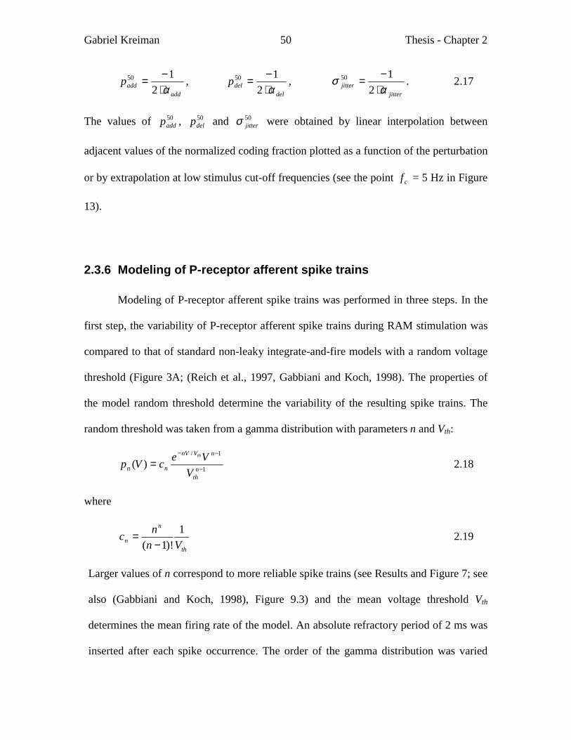
Gabriel Kreiman Thesis - Chapter 2
50
addaddp
α⋅−=
2150 ,
deldelp
α⋅−=
2150 ,
jitterjitter α
σ⋅−=
2150 . 2.17
The values of 50addp , 50
delp and 50jitterσ were obtained by linear interpolation between
adjacent values of the normalized coding fraction plotted as a function of the perturbation
or by extrapolation at low stimulus cut-off frequencies (see the point cf = 5 Hz in Figure
13).
2.3.6 Modeling of P-receptor afferent spike trains
Modeling of P-receptor afferent spike trains was performed in three steps. In the
first step, the variability of P-receptor afferent spike trains during RAM stimulation was
compared to that of standard non-leaky integrate-and-fire models with a random voltage
threshold (Figure 3A; (Reich et al., 1997, Gabbiani and Koch, 1998). The properties of
the model random threshold determine the variability of the resulting spike trains. The
random threshold was taken from a gamma distribution with parameters n and Vth:
1
1/
)( −
−−
= nth
nVnV
nn VVecVp
th
2.18
where
th
n
n Vnnc 1
)!1( −= 2.19
Larger values of n correspond to more reliable spike trains (see Results and Figure 7; see
also (Gabbiani and Koch, 1998), Figure 9.3) and the mean voltage threshold Vth
determines the mean firing rate of the model. An absolute refractory period of 2 ms was
inserted after each spike occurrence. The order of the gamma distribution was varied
Gabriel Kreiman Thesis - Chapter 2
51
between 1 (corresponding to an exponential distribution leading to Poisson distributed
spike times), 3, 5, 10 and 100 (effectively implementing the limit ∞→n , which
corresponds to a perfect integrator). The mean voltage threshold value, Vth, was fixed so
as to match the mean firing rate of the model to the one of each P-receptor afferent. 10
repetitions of the same RAM used to stimulate P-receptor afferents were fed to each
model and the distances between spike trains were computed as explained above.
In the second step, the linear transfer properties of P-receptor afferents were
characterized using a model based on an earlier one proposed by (Nelson et al., 1997) for
P-receptor afferents of Apteronotus leptorhynchus (see Figure 3B). An alternative
biophysical model proposed by (Kashimori et al., 1996) was not considered here, as our
goal was to obtain the simplest possible description of P-receptor afferent spike trains
taking into account their linear transfer function and the variability of their spike trains.
The stimulus was passed through a first order high pass filter with transfer function H(s),
ca
a Gs
sGsH +
+=
τ/1)( 2.20
simulating the linear transfer properties of P-receptor afferents. In this equation, Ga and
Gc are gain and offset terms, respectively, τa is the time constant of the filter and
ifis πω 2== is the complex circular frequency of the input signal. The parameters Ga,
Gc and τa were obtained by fitting the gain )2()( ifHfG π= and the phase
))2(Re)2(Im(tan)( 1 ifHifHf ππφ −= of the model to experimentally measured gains
and phases obtained from responses to sinusoidal amplitude modulations (SAMs). For
each SAM stimulus, the mean instantaneous firing rate was computed over the full
stimulus cycle and fitted to the function
Gabriel Kreiman Thesis - Chapter 2
52
ctfGtmfr fsf ++= )2sin()( φπ 2.21
(see Results and Figure 14). The fit parameters sfG and
sfφ are the experimental gain and
phase at the frequencies sf used in the SAMs protocols, respectively (see Stimulation
above). The constant c represents an offset between stimulus and response.
In the third and last step, the variability characterized in the first step and the
linear filtering properties obtained in the second step were combined to obtain a complete
model reproducing both the variability of P-receptor afferents and their linear filtering
properties. The high-pass filtered signal was delayed by 2.5 ms (corresponding to the
synaptic delay between tuberous receptors and afferent fibers) and a mean spontaneous
activity was added (Nelson et al., 1997; see Figure 3B). The resulting signal, z(t), was
then passed through a clipping non-linearity, effectively half-wave rectifying it and
imposing a maximal firing rate of 1 spike per EOD cycle,
)( =tr .)( if
,)(0 if )(,0)( if 0
EODEOD
EOD
ftzfftztz
tz
≥≤≤
< 2.22
The output, r(t) (see Figure 3B), was fed as input to a perfect integrator with gamma
distributed threshold, as described above, to determine when a spike was fired. The order
n of the gamma distribution for the threshold was selected to match the spike train
variability in response to SAMs, as assessed by computing interspike interval
distributions and distances between spike trains (see above and (Gabbiani and Koch,
1998)). The responses to RAM stimuli, when available, were then compared to the model
predictions (see Results). In some cases the mean firing rate of the model was adjusted to
take into account changes in the experimental firing rate during a recording session.
Gabriel Kreiman Thesis - Chapter 2
53
In the subsequent sections, we use the notation std to stand for standard
deviation and sem for standard error of the mean.
2.4 Results
This study is based on recordings and analysis from 69 P-receptor afferent fibers
obtained in 34 different animals.
2.4.1 Responses of P-receptors to repeated presentations of
identical RAMs
To investigate the variability of P-receptor afferent spike trains and its relation to
the encoding of electric field amplitude modulations, we recorded their responses to
repeated presentations of identical random amplitude modulations (RAMs) of a
sinusoidal electric field. The mean firing rates of afferent fibers were widely distributed,
ranging from 25 spike/s to 374 spike/s (mean ± std: 117 ± 69 spike/s). The coefficient
of variation of the interspike interval (ISI) distribution (CV = mean/std) ranged from 0.16
to 1.7 (mean ± std: 0.59 ± 0.36). These values were similar to those observed in
spontaneously active units (range: 0.12-1.12; (Wessel et al., 1996), Figure 2B2), although
several units analyzed here had higher CVs under RAM stimulation than those observed
spontaneously.
Figure 4 illustrates the range of responses to repeated RAMs recorded under a
variety of stimulus conditions and mean firing rates. In a few cases, the responses of P-
receptor afferents were highly reproducible from trial to trial (see in particular Figure 4C
Gabriel Kreiman Thesis - Chapter 2
54
and, to a lesser extent, Figure 4D) as has sometimes been observed in other preparations
(Mainen and Sejnowski, 1995, Bair and Koch, 1996, Berry et al., 1997). A clear locking
of the responses to the stimulus was usually observed at high contrasts ( 200>σ mV)
and cut-off frequencies ( 40>cf Hz; see Figure 4C, D). Furthermore, the mean firing
rate of the afferent fibers had to be low ( 125< spike/s; compare Figure 4C and G).
Decreasing the cut-off frequency or the stimulus contrast tended to decrease the
reproducibility of the spike occurrence times (Figure 4A, B). At high firing rates (> 125
spike/s), P-receptor afferent responses did not show clear trends of changes in
reproducibility with stimulus parameters (Figure 4E-H). These preliminary observations
suggested that the variability across trials of P-receptor afferent spike trains depended on
stimulus parameters as well as on the mean firing rate of the units.
2.4.2 Quantification of response variability
The spike count variance over short time windows has often been considered as
an indicator of spike train variability across repeated trials of the same stimulus (Berry et
al., 1997, van Steveninck et al., 1997). As a first step in quantifying P-receptor afferent
spike train variability, we therefore plotted the spike count variance vs. mean spike count
across trials in windows of various sizes (10, 50 and 100 ms) as illustrated in Figure 5. At
low firing rates (Figure 5, top row) the observed mean spike count in a given window
was typically low (<10 spikes per window) and the variance across trials as a function of
the mean had a scalloped appearance, reproducing almost perfectly a series of parabolas
stacked onto each other along the vertical axis. Similar observations have been made in
other preparations (in ganglion cells of the salamander retina, (Berry and Meister, 1998);
Gabriel Kreiman Thesis - Chapter 2
55
in a wide-field visual tangential neuron of the fly lobula plate, (van Steveninck et al.,
1997)). The lowest series of parabolas corresponded to the minimal possible variance that
is achieved when the spike count is either equal to n or n+1 (where n is an integer) in a
given window (see Methods). Higher parabolas corresponded successively to all spike
counts equal to n or 1+n , except for one equal to 1−n (or n+2), etc… per window. This
result indicated that the number of spikes per window was reliable (either n , 1+n or
1−n ) and well below that expected for a Poisson process (mean equals variance; dashed
line in Figure 5). However, since the scalloping was observed independently of the
stimulus cut-off frequency, it did not correlate with the reliability of spike occurrence
times, as observed in spike rasters (see Figure 4A-D). At higher firing rates, the mean
spike count reached up to 25 spikes or more per window (Figure 5, bottom row) and the
variance increased considerably, ranging from the theoretical minimum up to the mean
equals variance line. On average, the variance was still below that of a Poisson process.
Thus, according to the experimental results plotted in Figure 5, scalloping did not
appear to be directly related to the precision of spike timing across trials. To confirm this
point, we artificially modified the spike trains obtained in response to repeated
presentations of identical RAMs to alter the precision in spike timing without changing
the statistical properties of the spike trains. We took the 10 rasters of units exhibiting
scalloping of the spike count variance vs. mean spike count relation and firing with
varying degrees of reliability in response to RAMs (such as the rasters for the unit
illustrated in Figs. 4A, C and 5A-D) and successively shifted the spikes with a fixed
delay shiftt . In other words, if )(1 tx , …, )(10 tx represent the original spike trains, new
spike trains were defined as )()(~11 txtx = , )()(~
22 shiftttxtx += , …,
Gabriel Kreiman Thesis - Chapter 2
56
)9()(~1010 shiftttxtx ⋅+= . The parameter shiftt took three values: 1, 5 and 10 ms. We then
computed the variance vs. mean relations exactly as in Figure 5. In all cases (5 units, 14
conditions) and irrespective of whether the timing of spikes was reliable or not, the
scalloping remained present, independently of the value of shiftt . In some cases the
number of vertical rows of parabolas increased with shiftt . These points are illustrated in
Figure 6A and B. Similar results were obtained in integrate-and-fire neuron models as
illustrated in Figure 6C and D. Thus, in the worst case, 10=shiftt ms, the timing of spikes
drifted by 90 ms between the first spike train )(~1 tx and the last spike train )(~
10 tx without
affecting the scalloping in windows of 10, 50 and 100 ms. Since it was possible to largely
eliminate any precision in the spike occurrence times from trial to trial without altering
the scalloping of the spike count variance, this analysis confirmed that scalloping in these
time windows was not related to the reliability of spike occurrence times.
Because the spike count variance as a function of mean spike count did not offer a
reliable indication of spike train variability under our experimental conditions, we turned
to a second measure based on the calculation of distances between spike trains obtained
under repeated RAM stimulation. This measure, )(qDn , depends on a parameter q (in
units of 1/time) which determines the temporal precision at which the distance between
two spike trains is computed (higher values of q correspond to higher temporal
precisions, see Methods). For two identical spike trains 0)( =qDn independent of q. The
maximum, 1)( =qDn , is obtained for large values of q only if no spikes in the two spike
trains occurred exactly at the same time. The value at which 21)( =qDn , called 21q ,
may be used to summarize spike train variability: if we set 2/11 qt jitter = then jittert

Gabriel Kreiman Thesis - Chapter 2
57
measures the average time by which spikes have to be moved to transform one spike train
into the second one, or equivalently, the average jitter in spike timing. By definition, this
jitter also takes into account differences in spike numbers between the two spike trains
(i.e., the need to create or delete spikes to transform one spike train into the other; see
Methods and Figure 1).
We computed the average distance between all pairs of spike trains obtained in
response to the same RAM stimulus for our sample of 69 P-receptor afferents. The spike
train distances )(qDn were compared to those obtained from a family of gamma neuron
models indexed by a parameter n controlling spike train variability (see Methods). A
value of n = 1 (gamma-1 neuron) corresponds to Poisson distributed spike occurrence
times in response to the stimulus while for large n (n > 100) the gamma model is identical
to an integrate-and-fire neuron. Figure 7A illustrates in one example how the variability
observed in P-receptor afferents compared to the model variability. The top 10 rasters
labeled ‘P-unit’ correspond to the response of a P-receptor afferent while the next 10
rasters were obtained by simulating a Poisson (gamma-1) model. The P-receptor afferent
spike trains are considerably more regular than those of a Poisson neuron and match quite
well those of the gamma-10 model illustrated at the bottom of Figure 7A. Accordingly,
the average distance between two spike trains of this P-receptor afferent followed closely
that of the gamma-10 neuron (see Figure 7B, triangles and squares) and was always
smaller than the corresponding distance in a Poisson model (Figure 7B, circles). The
value )0(nD in Figure 7B yields the average difference in spike number between two
spike trains normalized by the total spike count. The small distance value, 02.0)0( =nD ,
indicates that the number of spikes was very reproducible from one trial to the next with

Gabriel Kreiman Thesis - Chapter 2
58
an average variability of 2%. On the other hand, )20(nD is the fraction of non-coincident
spikes in two spike trains at 0.1 ms resolution. The value 98.0)20( =nD in this
experiment indicates that less than 2% of spikes occurred at the same time ( ± 0.05 ms)
and thus the spike trains were clearly not reproducible at a 0.1 ms resolution. The average
temporal jitter in spike occurrence times, jittert , was in this case equal to 2.9 ms (with
86% of spikes moved and 14% of spikes added or deleted), corresponding to 1.3 EOD
cycles ( 438EOD =f Hz). Furthermore, the largest deviation between )(qDn in the
gamma-10 model (or the P-receptor afferent) and the Poisson model was observed for q
values lying in the interval 0.05 ms-1 – 0.25 ms-1 (Figure 7C). A value of q = 0.25 ms-1
was used to illustrate our results in subsequent figures.
Similar results were obtained in all 69 P-receptor afferents analyzed. The relative
difference in spike count, )0(nD , ranged from 0.01 to 0.1 (mean ± std: 0.03 ± 0.04),
while the fraction of non-coincident spikes, )20(nD , ranged from 0.87 to 1.0 (mean ±
std: 0.97 ± 0.04). The distribution of average temporal jitters is plotted in Figure 8A for
69 P-receptor afferents. The range of values was between 0.6 and 23.2 ms (mean ± std:
3.5 ± 3.9) with 77 ± 7% of spikes moved (mean ± std; range: 62 – 87%) and 23 ± 7%
of spikes added or deleted (mean ± std; range: 13 – 38%). Figure 8B re-plots the average
temporal jitter in units of the EOD cycle ( EOD1 f ) as measured for each fish prior to the
experiment. The temporal jitter ranged from a fraction of the EOD cycle (0.29) up to
several cycles (8.7; mean ± std: 1.4 ± 1.5). The temporal jitter was dependent on the
firing rate of the afferent fibers. High firing rate afferents (arbitrarily defined as those
with mean firing rate above 125> spike/s) had a mean jitter, jittert , of 1.7 ± 0.3 ms
Gabriel Kreiman Thesis - Chapter 2
59
(mean ± std; range: 0.6 – 2.45 ms) corresponding to 0.8 ± 0.3 EOD cycles (mean ± std;
range: 0.3-1.2). The mean jitter of low firing rate afferents ( 125< spike/s) was typically
higher, 6.3 ± 6.0 ms (mean ± std; range: 1.7 – 23.2 ms) corresponding to 2.4 ± 2.3
EOD cycles (mean ± std; range: 0.7 - 8.7).
2.4.3 Dependence of temporal jitter on stimulus cut-off frequency
Next, we investigated the dependence of spike timing jitter on stimulus
parameters and P-receptor afferent firing rates. Figure 9A illustrates the change in
temporal jitter as a function of cut-off frequency for a low firing rate unit (mfr = 65
spike/s). When the stimulus cut-off frequency was increased from 5 to 40 Hz, the timing
jitter decreased 1.4-fold from 4.8 ms to 3.5 ms. This increase in spike timing precision
was quantified by the slope of linear regression lines fitted to the data (see Figure 9A,
dashed line). As illustrated in Figure 9B, an increase in temporal precision was observed
mainly for units firing at low rates. The left panel shows the distribution of slopes for
units with a mean firing rate below 125 spike/s and the right panel the distribution of
slopes for units with mean firing rates above 125 spike/s. The slopes calculated for low
firing rate units were negative on average (mean ± std: -0.052 ± 0.066 ms/Hz) and
significantly different from 0 ( 05.0<p , 2-tailed t-test) while they were not significantly
different from zero at high firing rates (mean ± std: 0.01 ± 0.02 ms/Hz; 4.0>p ).
Correspondingly, correlation coefficients between cf and jittert were negative at low
rates (mean ± std: -0.59 ± 0.35) but not at high firing rates (mean ± std: 0.29 ± 0.62).
Gabriel Kreiman Thesis - Chapter 2
60
Similar results were obtained for the distance measure )(qDn over a broad range
of the spike distance parameter q , as illustrated in Figure 10. At fixed, intermediate
values of q , the average distance decreased as a function of stimulus cut-off frequency
for low-firing rate units (Figure 10A-C). At low temporal resolution (i.e., when q = 0 ms-
1 and )(qDn measures differences in spike counts) the slopes and correlation coefficients
of )(qDn vs. cf regression lines were not significantly different from 0 ( p > 0.2 at q =
0 ms-1, 2-tailed t-test). That is, no trend in spike count variability vs. stimulus bandwidth
could be observed. The same result was true at very high temporal resolution ( p > 0.2 at
q = 20 ms-1). At intermediate temporal resolutions, units firing at high rates did not show
slopes or regression coefficients significantly different from zero ( q in the range 0.05 –
0.75 ms-1; p > 0.05) while low firing rate units yielded a significant decrease in
variability with stimulus bandwidth ( p < 0.01 over the same range of values). The
strongest tendencies were observed for values of q between 0.25 and 0.5 ms-1 (Figure
10B, C).
2.4.4 Variability and stimulus contrast
The dependence of spike time jitter on stimulus contrast was very similar to the
one found for stimulus cut-off frequency. Figure 11A illustrates an example of a low
firing rate P-receptor afferent for which spike timing jitter decreased 2-fold as the
stimulus contrast was changed from 10% to 30%. The effect of stimulus contrast on spike
timing jitter is summarized in Figure 11B which reports the slopes of linear regression
Gabriel Kreiman Thesis - Chapter 2
61
lines for jittert vs. σ in P-units firing at low and high rates (left and right panels,
respectively). Increasing stimulus contrast was generally less effective than increasing
cut-off frequency at reducing spike time jitter as may be seen from the larger fraction of
units with slopes close to zero, even at low firing rates.
Figure 12 reports the same results directly in terms of spike train distances at all
values of q used. At low firing rates and for intermediate values of the temporal
resolution parameter, the average distance between two spike trains decreased as a
function of stimulus contrast (Figure 12A). Accordingly, the slopes of linear regression
lines and their correlation coefficients were significantly different from zero for low
firing rate units ( p < 0.01, 2-tailed t-test) but not for high firing rate units ( p > 0.05) at
those values of q (Figure 12B, C). At very low or very high temporal resolution ( q = 0
or 20 ms-1) changes with stimulus contrast were not statistically significant ( p > 0.05).
In summary, the study of spike train distances demonstrated that the timing
precision of P-receptor afferents increased with stimulus cut-off frequency and, to a
lesser extent, with stimulus contrast. Low firing rate units appear to be less variable than
high firing rate units.
2.4.5 Robustness of stimulus encoding
To assess the impact of alterations in spike timing on the accuracy of RAMs
encoding, we modified experimental spike trains by randomly adding, deleting or moving
spikes. The stimuli were then estimated from the modified spike trains (see Figure 2B
and Methods) and the change in coding fraction was monitored. The inset of Figure 13
Gabriel Kreiman Thesis - Chapter 2
62
reports in one example the fraction of the stimulus encoded as a function of spike time
jitter, normalized by its baseline value, the coding fraction of the original spike train. In
most cases the addition and the deletion of spikes or the addition of spike time jitter
resulted in a linear decrease of the normalized coding fraction as the perturbation
parameter was increased. Correlation coefficients ranged from 0.80 to 0.97 for 96% of
the data. In those cases, the robustness of encoding was characterized by the perturbation
value required to cause a 50% drop in coding fraction (see Figure 13, inset for the
definition of 50jitterσ ). P-receptor afferent spike trains were in general quite robust to such
perturbations. As illustrated in Figure 13, at low cut-off frequencies, spike time jittering
as high as 125 ms was required to cause a 50% drop in γ . The robustness to spike time
jitter decreased as the stimulus cut-off frequency increased, reaching a value of 6 ms for
fast changing stimuli ( cf = 88 Hz). The robustness to spike additions or deletions did not
show a dependency on stimulus bandwidth for cf > 5 Hz (see Table 1). For those stimuli,
a drop of 50% in the coding fraction was obtained after 36% random spike deletions and
41% additions. Robustness was not significantly dependent on stimulus contrast (data not
shown).
2.4.6 Modeling of P-receptor afferent variability and linear transfer
properties
The results reported above were summarized by building a model of P-receptor
afferent spike trains able to account for the encoding of RAMs and the spike train
variability observed experimentally across trials (see Figure 3 and Methods). We used an
Gabriel Kreiman Thesis - Chapter 2
63
approach similar to the one adopted by Nelson et al. (1997) in modeling P-receptor
afferents of Apteronotus leptorhynchus. The transfer functions of P-receptor afferents
have been described as high-pass in the species of weakly electric fish investigated so far
(Bastian, 1981, Nelson et al., 1997). We confirmed this and characterized quantitatively
the transfer function in Eigenmannia by recording responses to sinusoidal amplitude
modulations (SAMs). Gains and phases were extracted from linear fits to sinusoids
(Figure 14A and equation 8 in Methods) at various frequencies sf . The experimental
gains and phases were then fitted by maximum likelihood to a first order high-pass filter
(Figure 14B and equation 7). The resulting fits had 2χ -values divided by the number of
degrees of freedoms ( DOF2χ ; Press et al. 1992, chap. 15) for the fits between 0.7 and
8.0 (for 15 afferent fibers), except for two outliers ( DOF2χ = 22.8 and 24.2,
respectively). The mean values of the filter parameters were: aG = 120 ± 82 spikes/s
(range: 16-300 spikes/s), cG = 40 ± 26 spikes/s (range: 7-99 spikes/s) and aτ = 4 ± 5
ms (range:0.2-17.5 ms). In contrast to the results of Nelson et al. (1997) in Apteronotus,
fitting the data with a second order filter improved only slightly the DOF2χ -values of
the fits (range: 0.4 – 6.2). Since the additional parameters were not well constrained, this
approach was not pursued further. The static non-linearity illustrated in Figure 3B was
needed in the model to prevent z(t) from becoming negative, leading to firing rates lower
than those observed experimentally. The variability of P-receptor afferent spike trains
was estimated from repeated presentations of SAM stimuli and was in the same range as
the one observed for RAMs.
Gabriel Kreiman Thesis - Chapter 2
64
The ability of the model to predict responses to RAMs was tested in 10 P-receptor
afferents by computing coding fractions and spike train distances as a function of
stimulus contrast and cut-off frequency. Figure 15 illustrates two examples for a P-
receptor afferent firing at low rate (left panels, A-D) and a second P-receptor afferent at
high firing rate (right panels, E-H). The model successfully reproduced both the
dependence of coding fraction and spike train distances observed experimentally on cf
and σ .
2.5 Discussion
We characterized the variability of P-receptor afferent responses to RAMs under a
variety of stimulus conditions using a new measure of distance between spike trains. Our
results provide insight into the relationship between the variance in the number of spikes
and the mean spike count as a measure of variability across repeated trials. They also
shed light on the impact of variability on the processing of electric field amplitude
modulations by the electrosensory system in weakly electric fish.
2.5.1 Quantification of spike train variability
Spike train variability has often been quantified by computing the spike count
variance as a function of the mean spike count in fixed windows of length T (for a
review, see (Teich et al., 1996)). The benchmark stochastic process to which these values
are compared is the Poisson process for which the generation of independent spikes
yields a variance equal to the mean. The spike count variance provides an appropriate
measure of neural noise in tasks where the mean spike count (averaged over T) is used to
Gabriel Kreiman Thesis - Chapter 2
65
assess a neuron’s ability to discriminate between two alternatives (for reviews, see
(Gabbiani and Koch, 1998); (Parker and Newsome, 1998)). For long time intervals
( 1≥T s) variances larger than mean spike counts are often observed, indicative of
positive long-term correlations in the spike trains (Teich et al., 1996). Such time windows
are, however, inadequate to assess the ability of neurons to convey information about
time-varying stimuli by rapid changes in instantaneous firing rate.
Recently, the spike count variance has also been used as a measure of variability
at short time scales ( 300≤T ms; (Berry et al., 1997); (van Steveninck et al., 1997);
(Warzecha et al., 1998)). In our data, minimal non-zero values for the spike count
variance were observed in windows smaller than 100 ms, as has been reported in these
studies. However, they were not correlated with the reliability of spike occurrence times
assessed from raster plots (such as stimulus-dependent phase-locking to the sinusoidal
carrier signal) or with objective measures of the information encoded in the time-varying
firing rate like the coding fraction (Figure 4-6). Therefore, reliable spike timing is not a
necessary prerequisite for minimum non-zero variance curves: they may be observed
independently of whether spike timing is reproducible at the millisecond level from trial
to trial or not. Such curves should therefore be interpreted with caution (see also
(Warzecha and Egelhaaf, 1999), footnote 21; (Barberini et al., In Press)). One effect
leading to variances smaller than the mean over short time windows is the presence of a
refractory period that introduces negative correlations between spike occurrence times.
The addition of a refractory period to a Poisson stochastic process has recently been
shown to be sufficient to account for the variability observed in retinal ganglion cells
under dynamic stimulation (Berry and Meister, 1998). Similar observations were made in
Gabriel Kreiman Thesis - Chapter 2
66
other preparations (for a review, see (Johnson, 1996)). Figure 7B shows that a simple
Poisson process with a 2 ms refractory period driven by the stimulus did not reproduce
the spike train variability of P-receptor afferents. A comparison of variance vs. mean
spike count with theoretical results (Vannucci and Teich, 1981) suggests that the
regularizing effect of the refractory period is not sufficient to account entirely for the low
variability observed in our data. In addition to the refractory period, the generation of
spikes in P-receptor afferents appears to be governed by biophysical mechanisms that
exhibit intermediate levels of variability lying between those of Poisson and perfect
integrate-and-fire models and corresponding to the factors n=3-10 of our gamma-models .
Because of their mathematical definition and properties, the distances )(qDn and
the average timing jitter jittert are well suited to characterize the reproducibility of spike
occurrence times from one trial to the next. These measures are equally effective with
deterministic or random stimuli and are applicable in cases, such as here, where simpler
measures like the timing precision or reliability cannot be used (see Figure 4; (Bair and
Koch, 1996); (Berry et al., 1997)). By definition, the average jitter jittert is a measure that
automatically incorporates possible differences in spike number between two spike trains.
For example, since on average 23% of the spikes had to be added or deleted to transform
one spike train to a second one in our data set (see Results, Quantification of response
variability, last paragraph), the average time interval by which the remaining spikes were
moved was actually smaller by 15% than that reported in Figure 8. This may be seen
from equations 3 and 4: if αn and/or βn are different from zero, the parenthesis on the
right hand side of equation 4 will be smaller than one (= 0.85 in the present case),
implying that jittert = 2/11 q is larger than the average time interval given by the left hand
Gabriel Kreiman Thesis - Chapter 2
67
side of equation 4. The additional 15% increase in jittert converts the added or deleted
spikes into an effective time jitter equivalent.
Our use of spike time distances is different from the one originally introduced by
Victor and Purpura (1996, 1997). These authors employed spike train distances to assess
the information conveyed by stimulus-dependent clustering of spike trains from neurons
of the monkey visual cortex. In the present study, spike distances were used only to
assess the variability across identical trials; the performance at conveying stimulus-
dependent information was monitored with a second, independent measure, the coding
fraction.
2.5.2 Variability under various stimulus conditions
The results illustrated in Figs. 9-12 show that the timing precision of P-receptor
afferent spikes increases with the cut-off frequency of the stimulus and, to a lesser extent,
with the contrast of the RAMs. These results are consistent with observations made in
other preparations reporting that fast transients are likely to increase the precision of
spike occurrence times (Mechler et al., 1998, Berry et al., 1997, Warzecha et al., 1998).
Similarly, our findings that spike trains can be more reproducible at low than at high
firing rates (see Figure 4) is consistent with earlier observations (Berry et al., 1997, van
Steveninck et al., 1997, Warzecha and Egelhaaf, 1999). In contrast, no significant
differences in reliability were observed for RAM or SAM stimuli. Under the assumption
that the RAMs employed here are closer to natural stimuli than SAMs (van Steveninck et
al., 1997), our results do not support the idea that spike timing is more reliable under
natural stimulation (Warzecha and Egelhaaf, 1999). Behavioral experiments show that
Gabriel Kreiman Thesis - Chapter 2
68
Eigenmannia is able to perform remarkably precise jamming avoidance behaviors under
artificial stimulation (for a review, see (Kawasaki, 1997)). Accordingly, the reliability of
spike timing recorded in the time-coding pathway is very precise under such conditions.
In contrast to the amplitude-coding pathway, high reliability in the time-coding pathway
is necessary for the jamming avoidance response.
2.5.3 Variability and robustness of encoding
Our results show that the average jitter in the timing of P-receptor afferent spikes
jittert , is in most cases below 4 ms. On the other hand, the robustness of encoding to spike
time jitter yields values of 50jitterσ well above 4 ms for most of the behaviorally relevant
range of stimulus cut-off frequencies (see Table 1). Even at high stimulus cut-off
frequencies (e.g., 60=cf Hz), a jitter of 4 ms leads to a relative decrease in coding
fraction of at most 18% (see Table 1: 1150 =jitterσ ms implies that 0.82ms) 4( =nγ ). A
similar observation is valid for spike additions and deletions. Therefore, the jitter
observed in P-receptor afferents is in a temporal range that does not significantly affect
the information transmitted by single spike trains for most units and stimulus conditions.
On the other hand, a small amount of spike time jitter is beneficial to improve the
stimulus estimate obtained from several independent spike trains by averaging. We
verified this by computing estimates of the stimulus from r = 2-10 spike trains (recorded
successively from one neuron) simultaneously (Kreiman et al., 1998, Kreiman et al.,
2000b). The coding fraction increased when additional spike trains were included and
started to saturate for r = 6-7 spike trains. This was evaluated by extending the Wiener-
Gabriel Kreiman Thesis - Chapter 2
69
Kolmogorov filtering procedure to allow for a separate filter for each spike train (see
equations in Chapter 3) and also by computing a spike density function (SDF) from the
successively recorded spike trains. An example of the improvement in coding fraction
upon adding successive spike trains to estimate the SDF is shown in Figure 2-16. Figure
2-16a illustrates a short segment of the reconstructed stimulus from a single repetition.
The reconstruction is quite accurate and yields a coding fraction of approximately 0.6.
Upon computing the SDF from the 10 available repetitions of the identical stimulus, the
estimated stimulus becomes almost undistinguishable from the actual one (Figure 2-16b)
and yields a coding fraction reaching almost 0.9. It is interesting to observe that the
coding fraction seems to saturate after approximately 6 spike trains. Thus, our results
suggest that the spike timing jitter of P-receptor afferents lies in a range for which the
information transmitted by single units (when assessed by linear estimation) is not
degraded (for the range of behaviorally relevant stimulus cut-off frequencies considered
here) but which still allows for improvement by averaging over a small number of
afferents. Additional experiments recording simultaneously from several P-receptor
afferents under repeated presentations of the same RAMs are needed to confirm this
result.
2.5.4 Variability and the processing of amplitude modulations in the
ELL
At the next stage of the amplitude-coding pathway, the information carried by P-
receptor afferent spike trains is processed by pyramidal cells of the electrosensory lateral
line lobe (ELL). These neurons represent the output elements of the amplitude pathway
Gabriel Kreiman Thesis - Chapter 2
70
and project to various higher order brain structures specialized in the processing of
electrosensory information. There are two types of pyramidal cells, E- and I-type, which
receive direct excitatory input and indirect input via inhibitory interneurons, respectively.
At least two transformations have been identified in the representation of amplitude
modulations between the afferent input and the pyramidal cell output to the ELL: 1) the
detection threshold of pyramidal cells for amplitude modulations appears considerably
lower than the one of P-receptor afferents (Bastian, 1981) and 2) E- and I-type pyramidal
cells appear less sensitive to the detailed time-course of amplitude modulations than P-
receptor afferents and seem to extract the occurrence of upstrokes and downstrokes in
amplitude modulations, respectively (Metzner et al., 1998). Both these transformations
are likely to play a role in the generation of electrolocation and electrocommunication
behaviors. In particular, understanding the origin and mechanisms of increased sensitivity
of pyramidal cells might contribute to explain jamming avoidance responses to extremely
weak amplitude modulations and the detection of small preys using the electric sense
(Kawasaki, 1997, Nelson and Maciver, 1999).
Some sort of averaging operation across several afferent fibers converging onto a
pyramidal cell is likely to contribute to this increased sensitivity (Bastian, 1981), as
discussed in the previous section. One biophysical mechanism specifically proposed to
enhance the sensitivity of E-type pyramidal cells to upstrokes in the amplitude
modulation wave-form is coincidence detection (Berman and Maler, 1999): in slices of
the ELL of Apteronotus, the stimulation of afferents in the deep fiber layer produces
compound post-synaptic potentials consisting of an initial, fast-rising excitatory post-
synaptic potential followed by an inhibitory post-synaptic potential which limits the time-

Gabriel Kreiman Thesis - Chapter 2
71
window of integration to less than 10 ms and could therefore act as a high-pass filter for
coincident spikes occurring within 1-2 EOD cycles of each other (Berman and Maler,
1998; see Softky, 1995 for a similar theoretical result). Our experimental results show
that under repeated RAM stimulation more than 77% of P-receptor afferent spikes will on
average occur within 1-2 EOD cycles of each other in response to the same amplitude
modulation (Figure 8B). Thus, within the range of stimulus parameters investigated in
this study, spike trains of P-receptor afferents appear indeed able to provide the
information necessary for such coincidence detection operations.
2.5.5 Encoding of biological signals and analog to digital conversion
Here we have discussed how a biological system has evolved to encode a time-varying
signal in the spike trains of neurons in the sensory periphery. The variations in the
electric field amplitude can be seen as an analog signal to be encoded by the digital spike
trains (given by the presence or absence of a spike at a given time). The problem of
encoding an analog signal in a digital format is a widely important one in signal
processing. According to the sampling theorem, a limited number of samples (given by
the Nyquist frequency) is sufficient to accurately encode a band-limited signal without
any information loss provided that we can store the actual value of the analog signal
(Oppenheim et al., 1997). When the data is digitized, there is a potential for loss of
information. One possible solution to this is to use many bits to encode each sampled
value (in the limit when the number of bits goes to infinity, the sampling theorem
applies.) But a binary processor can only encode the signal using a 0/1 value in each
sample. The key to this is oversampling, that is, sampling at a much higher frequency
Gabriel Kreiman Thesis - Chapter 2
72
than the Nyquist limit. Oversampled Σ∆ analog-to-digital converters can accurately
encode the incoming signal and are widely used in technological applications (Aziz et al.,
1996, Wong and Gray, 1990, Gray, 1995). Fabrizio Gabbiani noted the close relationship
between oversampled Σ∆ converters and many current models of neuronal processing
(Gabbiani and Metzner, 1999). A schematic diagram indicating the signal processing
steps in an oversampled Σ∆ analog to digital converter is shown in Figure 2-17. A clock
pulse regulates the time of generation of pulses, effectively sampling the input at a
frequency several times higher than the Nyquist value. Pulses are generated whenever the
integrated analog signal crosses a specified threshold. So far this is identical to the
process in an integrate-and-fire neuronal model (Koch, 1999). When a pulse is generated
the voltage is subtracted from the signal in the next integration step. This is slightly
different from the neuronal model where, after a spike, the voltage is typically reset to the
membrane voltage (normally set at zero). Another important difference is that a time
period is typically reserved in the neuronal model after a spike where no pulses can be
generated to account for the absolute refractory period. The model that we have presented
in this Chapter is based on the integrate-and-fire model with some modifications to fit the
transfer properties of P-receptor afferents and its variability (see Figure 2-3 and Section
2.3.6). Engineers therefore seem to have independently designed a method to encode
analog signals in a digital format that strongly resembles the processing performed in the
encoding of environmental time-varying signals in the sensory nervous system.
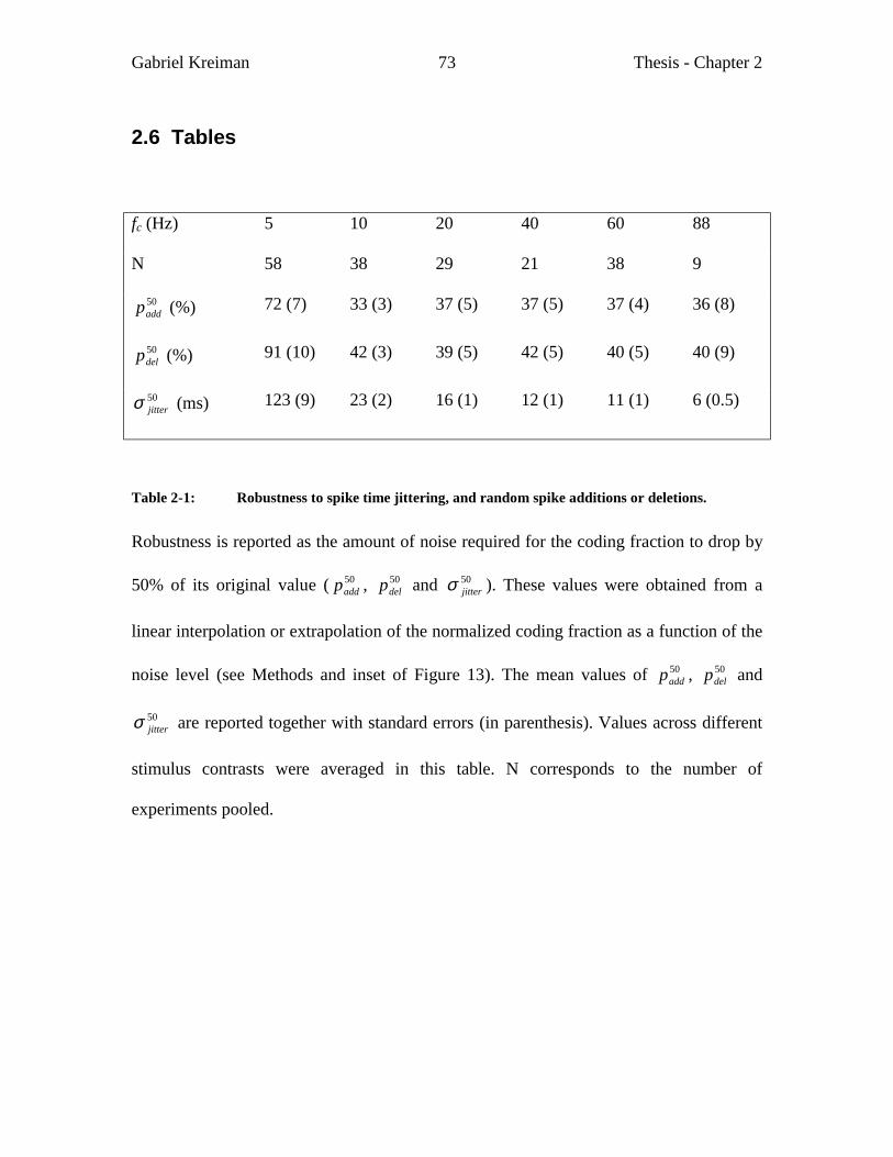
Gabriel Kreiman Thesis - Chapter 2
73
2.6 Tables
fc (Hz) 5 10 20 40 60 88
N 58 38 29 21 38 9
50addp (%) 72 (7) 33 (3) 37 (5) 37 (5) 37 (4) 36 (8)
50delp (%) 91 (10) 42 (3) 39 (5) 42 (5) 40 (5) 40 (9)
50jitterσ (ms) 123 (9) 23 (2) 16 (1) 12 (1) 11 (1) 6 (0.5)
Table 2-1: Robustness to spike time jittering, and random spike additions or deletions.
Robustness is reported as the amount of noise required for the coding fraction to drop by
50% of its original value ( 50addp , 50
delp and 50jitterσ ). These values were obtained from a
linear interpolation or extrapolation of the normalized coding fraction as a function of the
noise level (see Methods and inset of Figure 13). The mean values of 50addp , 50
delp and
50jitterσ are reported together with standard errors (in parenthesis). Values across different
stimulus contrasts were averaged in this table. N corresponds to the number of
experiments pooled.
Gabriel Kreiman Thesis - Chapter 2
74
2.7 Figure legends
Figure 2-1: Computation of spike train distances
The distance between two spike trains was obtained as the minimum cost to convert one
spike train into the second one using 3 elementary steps. A: The minimum cost path
transforming spike train 1 into spike train 8 is illustrated (for a fixed value of q). Each
intermediate spike train 2-7 corresponds to one elementary step: moving (from 2 to 3),
adding (from 6 to 7) or deleting (from 1 to 2) a single spike. The cost of each elementary
step is indicated on the right. Note that the cost of moving a spike is proportional to the
distance that it is moved along the time axis. B: There are two alternatives to go from
spike train 2 to spike train 3 in A. (i) Delete the last spike and add a new one or, (ii),
move the last spike to its new desired position. The latter alternative is less expensive for
the particular value of q illustrated here since 21 <∆⋅ tq (the dashed time interval of
length 2/q corresponds to the maximum displacement for which it is less expensive to
move a spike).
Figure 2-2: Quantification of stimulus encoding and of its robustness to spike time jittering.
A: An estimate, sest(t), of the stimulus s(t) was obtained from the spike train by
convolving it with a Wiener-Kolmogorov filter (see main text for details). The accuracy
of stimulus encoding by the spike train was assessed by computing the mean square error
(ε2) between the stimulus and the estimate. The brackets, ⋅ , denote averaging over time.
Gabriel Kreiman Thesis - Chapter 2
75
B: Temporal jitter was introduced by adding to each spike time a random variable taken
from a zero-mean gaussian distribution with standard deviation σjitter. The modified spike
trains are shown for increasing values of σjitter (from top to bottom) on the left. From each
distorted spike train, a new WK-filter and a new estimate, sest(t), of the stimulus were
computed (right). Robustness was quantified by computing the rate at which the fraction
of the stimulus encoded decreased with σjitter (see inset to Figure 2-13). A similar
procedure was used when spikes were randomly added or deleted from the spike trains.
Figure 2-3: Comparison of P-receptor afferent spike trains to integrate-and-fire models.
A: The variability of experimental spike trains was compared to the variability of perfect
integrate-and-fire (I&F) neurons with a random threshold. In this model, the sum of the
stimulus and a constant bias term (corresponding to the spontaneous activity) is
integrated and a spike is emitted each time that the threshold (Vthresh) is reached. After
each spike, a refractory period of 2 ms is imposed and a new threshold value is chosen
from a gamma probability distribution. B: To model the linear transfer properties of P-
receptor afferent spike trains, the amplitude modulation was first linearly filtered, with a
high-pass filter fitted from the responses of P-receptor afferent to SAMs (see Figure 2-
14) and then delayed. The output z(t) was clipped and injected into a perfect integrate-
and-fire neuron with random threshold and refractory period equal to 2 ms.
Figure 2-4: P-receptor afferent responses to RAMs exhibit a broad range of variability.
A portion of the stimulus presented to each P-receptor afferent is shown on top. Each
raster of spikes (9 per panel, 500 ms long) illustrates the response of the same P-receptor
Gabriel Kreiman Thesis - Chapter 2
76
afferent to a single presentation of the stimulus. The left column (A, C, E, G) illustrates
responses for fixed stimulus contrast (σ=250 mV) of a neuron with low mean firing rate
(A and C: mfr=65 ± 2 spike/s) and a different neuron with high firing rate (E, G: mfr=137
± 1 spike/s) to stimuli with low and high cut-off frequencies (A, E: fc=5 Hz; C, G: fc=60
Hz). The right column (B, D, F, H) illustrates the responses for a fixed cut-off frequency
(fc=60 Hz) of a neuron with low firing rate (B, D: mfr=62 ± 1 spike/s) and a different
neuron with high firing rate (F, H: mfr=151 ± 1 spike/s) to stimuli with low and high
contrasts (B, F: σ=100 mV; D, H: σ=275 mV).
Figure 2-5: Scalloping of the variance vs. mean spike count relation is not a predictor of spike
timing variability.
Plots of spike count variance vs. mean spike count in windows T of 10, 50 and 100 ms.
A-D were obtained in a neuron firing at low rate (mfr = 65 ± 2 spike/s), for fixed
contrast ( 250=σ mV) and various cut-off frequencies cf (as indicated on the top of
each panel; 5A is the same experiment as in Figure 4A). E-H were obtained in a different
neuron with high firing rate (mfr = 151 ± 1 spike/s) for the same contrast and cut-off
frequency values. Note that the variance vs. mean spike count curves follow the
theoretical minimum curves in A-D in spite of the fact that reliable spike timing was only
observed at high values of cf (see Figure 4A through D). At higher firing rates (E-H)
scalloping is still observed in some cases but is masked by a general increase in spike
count variability. The 3 clusters evident in G, H and to a lesser extent in F, correspond to
the 3 window sizes (if T varies continuously between 10 and 100 ms no clusters are
observed). In all panels mean equal to variance is indicated by a straight dashed line.
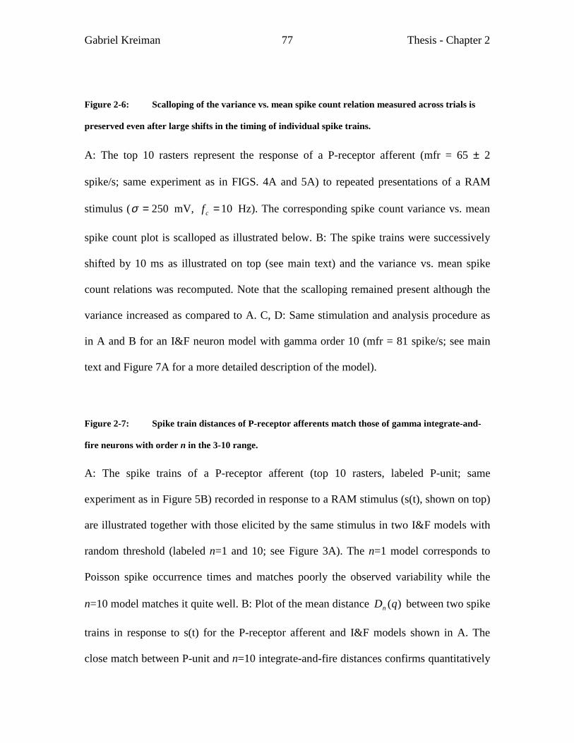
Gabriel Kreiman Thesis - Chapter 2
77
Figure 2-6: Scalloping of the variance vs. mean spike count relation measured across trials is
preserved even after large shifts in the timing of individual spike trains.
A: The top 10 rasters represent the response of a P-receptor afferent (mfr = 65 ± 2
spike/s; same experiment as in FIGS. 4A and 5A) to repeated presentations of a RAM
stimulus ( 250=σ mV, 10=cf Hz). The corresponding spike count variance vs. mean
spike count plot is scalloped as illustrated below. B: The spike trains were successively
shifted by 10 ms as illustrated on top (see main text) and the variance vs. mean spike
count relations was recomputed. Note that the scalloping remained present although the
variance increased as compared to A. C, D: Same stimulation and analysis procedure as
in A and B for an I&F neuron model with gamma order 10 (mfr = 81 spike/s; see main
text and Figure 7A for a more detailed description of the model).
Figure 2-7: Spike train distances of P-receptor afferents match those of gamma integrate-and-
fire neurons with order n in the 3-10 range.
A: The spike trains of a P-receptor afferent (top 10 rasters, labeled P-unit; same
experiment as in Figure 5B) recorded in response to a RAM stimulus (s(t), shown on top)
are illustrated together with those elicited by the same stimulus in two I&F models with
random threshold (labeled n=1 and 10; see Figure 3A). The n=1 model corresponds to
Poisson spike occurrence times and matches poorly the observed variability while the
n=10 model matches it quite well. B: Plot of the mean distance )(qDn between two spike
trains in response to s(t) for the P-receptor afferent and I&F models shown in A. The
close match between P-unit and n=10 integrate-and-fire distances confirms quantitatively

Gabriel Kreiman Thesis - Chapter 2
78
the visual observation in A (standard errors are too small to be visible, 90=pairsn ). C:
Plot of the difference in mean distances between n=1 and n=10 models (mean ± sem,
90=pairsn ) as a function of q. 10order
gammaPoisson )()()( qDqDqD nnn −=∆ , where Poisson)(qDn
corresponds to the filled circles in B and 10order
gamma)(qDn to the squares. Note that the largest
difference in distances is observed in the range of q values between 0.05 and 0.25 ms-1. In
B and C the value q = 20 ms-1 was not plotted because it would lie off-scale (see main
text).
Figure 2-8: Distribution of mean spike time jitter in 69 P-receptor afferents (corresponding to
508 different RAM stimulations).
A: Distribution of the average temporal jitter (bin size: 0.4 ms). For display purposes, the
probability distribution is shown only up to 10 ms; 8.2% of the cumulative distributions
lied between 10 ms and the maximal value observed (23.2 ms). B: Same distribution of
jittert in units of EOD cycles (2 bins per EOD cycle). In each panel, the arrows indicate
the means of the distributions.
Figure 2-9: The timing jitter decreases with stimulus cut-off frequency at low but not at high
firing rates.
A: Plot of the mean jitter in spike occurrence times as a function of stimulus frequency
for a neuron firing at low rate (mfr = 65 spike/s, 250=σ mV, 438EOD =f Hz;
percentage of spikes moved: 85 ± 3%). B: The slope of timing jitter vs. cut-off
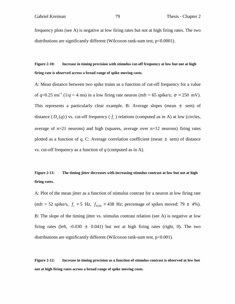
Gabriel Kreiman Thesis - Chapter 2
79
frequency plots (see A) is negative at low firing rates but not at high firing rates. The two
distributions are significantly different (Wilcoxon rank-sum test, p<0.0001).
Figure 2-10: Increase in timing precision with stimulus cut-off frequency at low but not at high
firing rate is observed across a broad range of spike moving costs.
A: Mean distance between two spike trains as a function of cut-off frequency for a value
of q=0.25 ms-1 (1/q = 4 ms) in a low firing rate neuron (mfr = 65 spike/s; 250=σ mV).
This represents a particularly clear example. B: Average slopes (mean ± sem) of
distance ( )(qDn ) vs. cut-off frequency ( cf ) relations (computed as in A) at low (circles,
average of n=21 neurons) and high (squares, average over n=12 neurons) firing rates
plotted as a function of q. C: Average correlation coefficient (mean ± sem) of distance
vs. cut-off frequency as a function of q (computed as in A).
Figure 2-11: The timing jitter decreases with increasing stimulus contrast at low but not at high
firing rates.
A: Plot of the mean jitter as a function of stimulus contrast for a neuron at low firing rate
(mfr = 52 spike/s, 5=cf Hz, 438EOD =f Hz; percentage of spikes moved: 79 ± 4%).
B: The slope of the timing jitter vs. stimulus contrast relation (see A) is negative at low
firing rates (left, -0.030 ± 0.041) but not at high firing rates (right, 0). The two
distributions are significantly different (Wilcoxon rank-sum test, p<0.001).
Figure 2-12: Increase in timing precision as a function of stimulus contrast is observed at low but
not at high firing rates across a broad range of spike moving costs.

Gabriel Kreiman Thesis - Chapter 2
80
A: Mean distance between two spike trains as a function of stimulus contrast for a value
of q = 0.25 ms-1 in a low firing rate neuron (mfr = 52 spike/s, 5=cf Hz, 438EOD =f
Hz). This represents a particularly clear example. B: Average slopes (mean ± sem) of
distance ( )(qDn ) vs. stimulus contrast (σ ) relations (computed as in A) at low (circles,
average over n = 23 neurons) and high (squares, average over n= 8 neurons) firing rates
as a function of q. C: Average correlation coefficient (mean ± sem) of distance vs. cut-
off frequency as a function of q (computed as in A and B).
Figure 2-13: Robustness of RAM encoding decreases with stimulus bandwidth.
Plot of the timing jitter (mean ± sem) causing a 50% reduction in the coding fraction as a
function of stimulus bandwidth. Averages were computed on n = 58, 38, 21, 22, 38 and 9
stimulus conditions from low to high cf , respectively (the large error at 5=cf Hz is due
to extrapolation from shallow slopes, see Methods for the computation of 50jitterσ ).
Figure 2-14: Fit of linear transfer function properties of a P-receptor afferent by a first order
high-pass filter.
A: Plot of the mean instantaneous firing rate as a function of the normalized period
fraction np (π2s
ntfp = , bin size: 1/20 of the period cycle) for 3 different sinusoidal
amplitude modulations ( 1=sf , 20 and 100 Hz, respectively). The solid line represents
the fit with equation 8 (see Methods; r2 is the correlation coefficient between the data and
fit). B: Fits of the mean gain and phase ( ± std) obtained from A (see equation 7) with a
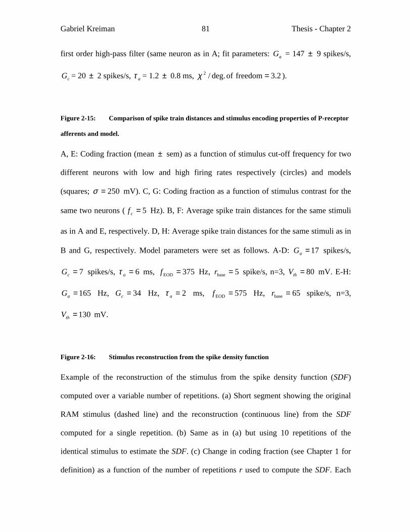
Gabriel Kreiman Thesis - Chapter 2
81
first order high-pass filter (same neuron as in A; fit parameters: aG = 147 ± 9 spikes/s,
cG = 20 ± 2 spikes/s, aτ = 1.2 ± 0.8 ms, 2.3freedom of deg./2 =χ ).
Figure 2-15: Comparison of spike train distances and stimulus encoding properties of P-receptor
afferents and model.
A, E: Coding fraction (mean ± sem) as a function of stimulus cut-off frequency for two
different neurons with low and high firing rates respectively (circles) and models
(squares; 250=σ mV). C, G: Coding fraction as a function of stimulus contrast for the
same two neurons ( 5=cf Hz). B, F: Average spike train distances for the same stimuli
as in A and E, respectively. D, H: Average spike train distances for the same stimuli as in
B and G, respectively. Model parameters were set as follows. A-D: 17=aG spikes/s,
7=cG spikes/s, 6=aτ ms, 375EOD =f Hz, 5base =r spike/s, n=3, 80=thV mV. E-H:
165=aG Hz, 34=cG Hz, 2=aτ ms, 575EOD =f Hz, 65base =r spike/s, n=3,
130=thV mV.
Figure 2-16: Stimulus reconstruction from the spike density function
Example of the reconstruction of the stimulus from the spike density function (SDF)
computed over a variable number of repetitions. (a) Short segment showing the original
RAM stimulus (dashed line) and the reconstruction (continuous line) from the SDF
computed for a single repetition. (b) Same as in (a) but using 10 repetitions of the
identical stimulus to estimate the SDF. (c) Change in coding fraction (see Chapter 1 for
definition) as a function of the number of repetitions r used to compute the SDF. Each
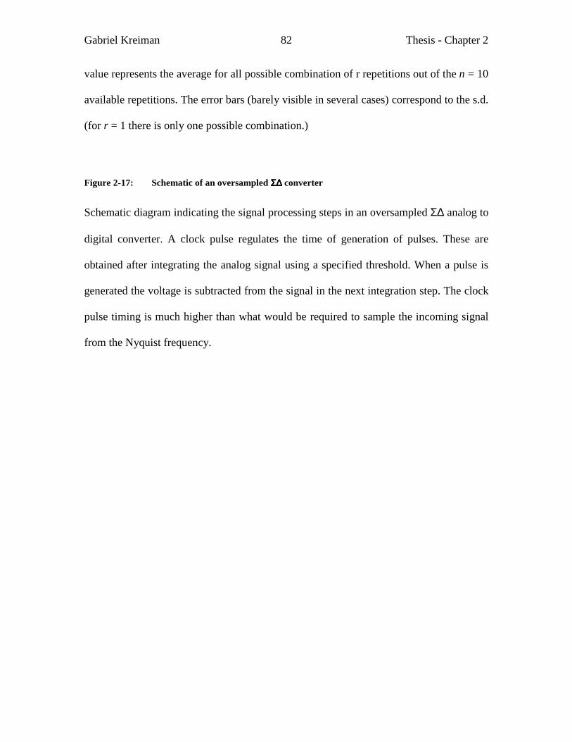
Gabriel Kreiman Thesis - Chapter 2
82
value represents the average for all possible combination of r repetitions out of the n = 10
available repetitions. The error bars (barely visible in several cases) correspond to the s.d.
(for r = 1 there is only one possible combination.)
Figure 2-17: Schematic of an oversampled ΣΣΣΣ∆∆∆∆ converter
Schematic diagram indicating the signal processing steps in an oversampled Σ∆ analog to
digital converter. A clock pulse regulates the time of generation of pulses. These are
obtained after integrating the analog signal using a specified threshold. When a pulse is
generated the voltage is subtracted from the signal in the next integration step. The clock
pulse timing is much higher than what would be required to sample the incoming signal
from the Nyquist frequency.

Gabriel Kreiman Thesis - Chapter 2
90
Figure 2-8

Gabriel Kreiman Thesis - Chapter 2
91
Figure 2-9

Gabriel Kreiman Thesis - Chapter 2
92
Figure 2-10

Gabriel Kreiman Thesis - Chapter 2
93
Figure 2-11

Gabriel Kreiman Thesis - Chapter 2
94
Figure 2-12

Gabriel Kreiman Thesis - Chapter 2
95
Figure 2-13

Gabriel Kreiman Thesis - Chapter 2
96
Figure 2-14

Gabriel Kreiman Thesis - Chapter 2
97
Figure 2-15

Gabriel Kreiman Thesis - Chapter 2
98
Figure 2-16

Gabriel Kreiman Thesis - Chapter 2
99
Figure 2-17
Gabriel Kreiman Thesis - Chapter 2
100
3 Stimulus encoding and feature extraction by multiple
sensory neurons
3.1 Overview
Are correlated responses of nearby neurons within topographic sensory maps
merely a sign of redundancy or do they carry additional information? To tackle this
problem we recorded simultaneously from pairs of electrosensory pyramidal cells with
overlapping receptive fields in the hindbrain of weakly electric fish. We found that: first,
nearby pyramidal cells exhibit strong correlations, mainly due to time-locking of spikes
to the stimulus. Second, stimulus estimation from simultaneous spike trains resulted in
significant improvements over single spike trains, but was still inferior to single primary
afferents. Third, in a feature-extraction task, coincident spikes of pyramidal cell pairs
performed significantly better than isolated spikes and even bursts of single cells.
Coincident spikes can thus be considered as “distributed bursts“. Our results suggest that
stimulus-induced coincident activity can improve the extraction of behaviorally relevant
features from the stimulus. At the time of writing this Thesis, the results of the current
Chapter are in press in the Journal of Neuroscience (Krahe et al., 2002).

Gabriel Kreiman Thesis - Chapter 3
101
3.2 Introduction
Different stimulus variables of complex sensory signals are mostly extracted in
segregated sensory pathways, often within structures that each contain a more or less
complete representation of the sensory epithelium. Such multiple sensory maps, which
are commonly found in many vertebrate sensory systems, exhibit various physiological
differences that are presumably correlated with their respective function in computing
different stimulus features (see for example (Konishi, 1991, Konishi, 1993, Konishi,
1995, Shumway, 1989b, Shumway, 1989a, Heiligenberg and Bastian, 1984,
Heiligenberg, 1991, Maunsell, 1995). A defining characteristic of topographic sensory
maps is that adjacent neurons process information about neighboring locations in the
sensory environment (for review see (Kaas, 1997, Wandell, 1995, Allman, 1999, Allman
and McGuinness, 1988, Kandel et al., 2000). Hence, the activity of nearby neurons is
often correlated (see for example (Usrey and Reid, 1999, Laurent, 1996, Singer and Gray,
1995). Do such neurons carry largely redundant information or can correlated activity
itself be useful? So far, several investigations have addressed this question by studying
stimulus encoding through the combined activity of multiple neurons, each of which
quite faithfully followed the stimulus time course (see for example (Warland et al., 1997,
Dan et al., 1998, Stanley et al., 1999, Nirenberg et al., 2001). Using pyramidal cells in the
hindbrain of weakly electric fish as a model system, we considered cells that do not
precisely follow the stimulus time course but rather appear specialized to extract stimulus
features.
Gabriel Kreiman Thesis - Chapter 3
102
Previous studies of information encoding in the electrosensory system showed
that single P-receptor afferents transmit up to 80% of the information on random
amplitude modulations (RAMs) of the electric field (see Chapter 1 and (Wessel et al.,
1996, Gabbiani and Metzner, 1999) Single pyramidal cells, however, encode the stimulus
time course only poorly. Instead, they reliably indicate the occurrence of upstrokes and
downstrokes in stimulus amplitude by bursts of spikes (Gabbiani et al., 1996, Metzner et
al., 1998). Extending this line of research to multiple pyramidal cells, we now asked three
questions: first, is the detailed information on the stimulus time course, which is available
from the primary afferent spike trains, indeed discarded at the level of the ELL, or can it
still be read from the combined activity of groups of pyramidal cells? Second, how
strongly correlated is the activity of pyramidal cells whose receptive fields overlap, and
what is the source of this correlation? Third, can correlations between spike trains of
multiple neurons enhance the extraction of stimulus features from the combined neuronal
activity?
To address these questions, we performed dual recordings in vivo from nearby
pyramidal cells in the centromedial map (CM) of the ELL and verified the overlap of
their receptive fields, while presenting RAMs of a mimic of the fish’s electric field. To
characterize correlations between spike trains of simultaneously recorded neurons we
applied cross-correlation analysis. Stimulus encoding and feature extraction were
quantified using reconstruction techniques and methods derived from signal-detection
theory, respectively (Metzner et al., 1998, Gabbiani et al., 1996, Rieke et al., 1997).
Gabriel Kreiman Thesis - Chapter 3
103
3.3 Methods
All the data described in the current Chapter were recorded by the laborious and
rigorous effort of Ruediger Krahe and Walter Metzner at the University of California at
Riverside.
3.3.1 Preparation and electrophysiology
The methods for preparation of the fish for electrophysiology followed the
guidelines described in Chapter 1. Initially, dual recordings from pyramidal cells were
obtained using two separate borosilicate glass micropipettes filled with 3 M KCl. After
recordings from 25 cell pairs we switched to Wood’s metal-filled glass micropipettes
with platinated tips. These extracellular single-unit recordings proved to be much more
stable, thus allowing us to determine whether the receptive fields of the two recorded
cells overlapped (see Section 3.3.3.)
Recordings for this study were restricted to pyramidal cell bodies within the
centromedial segment (CM.) The layer of pyramidal cell bodies is easily identified using
anatomical and physiological criteria (see (Metzner et al., 1998) The ELL is highly
laminated and the somata of large pyramidal cells are situated in a central layer that
extends dorso-ventrally over a distance of 200 µm. The CM layer can be identified easily
by anatomical and physiological criteria. For instance, the center of the pyramidal cell
layer is located ~ 200 µm dorsal to the spherical cell layer, which is only ~ 100 µm thick
and physiologically very distinct. Spherical cells are innervated by T-receptor afferents
and fire, in contrast to pyramidal cells, strictly phase locked to the ECOC mimic even at
Gabriel Kreiman Thesis - Chapter 3
104
the low stimulus amplitudes used in our study. This very reliable landmark permitted to
limit data collection to the pyramidal cell layer. Data collection from within CM was
verified by first physiologically mapping the border between the adjoining medial
segment (low-frequency sensitive) and CM and then inserting electrodes laterally only
within the adjacent 500 µm, which at this rostrocaudal level insures that penetrations do
not reach the laterally adjoining centrolateral segment. Initially, recording sites were also
verified histologically by setting small electrolytic lesions at the end of the experiment.
3.3.2 Anatomy
To measure the terminal spread of single P-receptor afferents in CM we
iontophoretically injected Neurobiotin (2% in 1 M KCl; Vector Laboratories,
Burlingame, CA) into the ganglion of the anterior lateral line nerve. After survival times
between 7 and 14 hours the animals were euthanized with MS222 (tricaine-methane
sulfonate; Sigma; pH 7) and perfused transcardially with saline followed by fixative (4%
paraformaldehyde in 0.1 M phosphate buffer.) The brains were postfixed overnight,
sectioned at 50 µm thickness, and then underwent a standard ABC (Vectastain Elite;
Vector Laboratories) and DAB reaction (Metzner and Juranek, 1997a). Terminal-spread
measurements were not corrected for shrinkage of tissue due to fixation. Axons which did
not contact spherical cells were classified as belonging to P-receptor afferents (Maler et
al., 1981, Maler, 1979, Carr et al., 1982, Heiligenberg and Dye, 1982). The nomenclature
of the brain structures used for the light-microscopic analysis follows (Maler et al.,
1991).
Gabriel Kreiman Thesis - Chapter 3
105
3.3.3 Stimulation
Stimuli were presented as described in Chapter 1 (see also (Kreiman et al.,
2000b). The parameter A0 (see Chapter 1) took values between 1 and 5 mV/cm measured
at the pectoral fin and perpendicular to the body axis. The stimuli, s(t), had a flat power
spectrum up to a fixed cutoff frequency (fc = 5, 10, 20 Hz; in some experiments cutoff
frequencies of 40 or 60 Hz were also used.) The standard deviation (or contrast), σ, of the
stimulus was 25% of the mean amplitude for all fc. For fc = 5 Hz, we additionally
presented contrasts of 10, 15, 20, and 27.5% if time permitted. The stimuli were D/A-
converted (pyramidal cellI-MIO16E-4, National Instruments, Austin, TX) at a sampling
rate of 5 kHz. Following lowpass-filtering (2 kHz; Wavetek Rockland Model 452,
Wavetek, San Diego, CA), a manual attenuator (839 Attenuator, Kay Elemetrics, Lincoln
Park, NJ) was used to adjust the final stimulus amplitude. The duration of the stimuli was
15 s, which is shorter than the duration of the stimuli used in earlier studies on pyramidal
cells (Gabbiani et al., 1996, Metzner et al., 1998). We therefore verified by cross-
validation that this optimized duration gave reliable results12.
In order to test if the receptive fields of two simultaneously recorded pyramidal
cells were overlapping, we positioned a local electrode (Shumway, 1989a) close to the
skin of the animal (see Figure 4-1; distance < 1 mm), and accepted a pair of cells only as
having overlapping receptive fields if both units gave robust responses to a sinusoidal
amplitude modulation of 5 Hz presented via the local electrode. The mouth electrode
12 If the stimulus is too short, it is possible to overfit the data upon computing the Euclidian feature and probability of misclassification. We therefore compared the results of the estimation of pe with segments of 15 second duration from data extracted randomly from the 30 seconds of recordings in the previous experiments (Metzner et al., 1998). It should also be noted that, in general, we used the same data to compute the Euclidian feature and pe. To verify that the degree of overfitting was small, we used a cross-validation procedure (Fukunaga, 1990) by dividing the data in two sets, one used for "training" (computing the Euclidian feature) and the other one for "testing" (computing pe given the Euclidian feature.)
Gabriel Kreiman Thesis - Chapter 3
106
served as the reference. We accepted cells for recording and analysis only when, for the
given stimulation site, they displayed center responses, that is they showed the same
response type (E or I) as for stimulation with the global field. Response strength
decreased dramatically within a few mm of the strongest center activity as reported
previously (Shumway, 1989a). Recording time did not permit a detailed mapping of the
extent of the receptive fields.
3.3.4 Cross-correlations
Let xA(n) and xB(n) represent two simultaneously recorded spike trains after
binning, where x(n)=1 if and only if there is a spike in bin n (n=1,...,N where N is the
total number of bins in the spike trains.) We computed the cross-correlograms between
the two pyramical cell spike trains given by:
BA
N
nBAAB xxnxnxR o≡+= ∑
−
=
τ
ττ1
)()()(
3.1
The spike trains as well as τ were binned using bin sizes of 3, 6 and 9 ms. The statistical
significance in departures from random coincident firing was assessed as described by
(Palm et al., 1988, Aersten et al., 1989, Perkel et al., 1967). Repeated presentations of
identical stimuli allowed us to compute the shuffle-correctors, where the cross-
correlograms were evaluated from successive, non-simultaneous repetitions, and
estimated the degree of departure of the shuffle-corrected correlograms from the null
hypothesis of independent firing (Palm et al., 1988, Aersten et al., 1989, Perkel et al.,
Gabriel Kreiman Thesis - Chapter 3
107
1967, Brody, 1997). The raw cross-correlogram was then computed by averaging the
correlograms in the individual repetitions, r (r = 1, ... , nrep):
∑=
=repn
i
rB
rA
repAB xx
nR
1
1)( oτ
3.2
This function evaluates the average correlated activity, including synchronous spikes as
well as stimulus-induced correlations. The expected value of R as well as the degree of
departures expected by chance can be easily evaluated (Perkel et al., 1967, Palm et al.,
1988). The stimulus-induced effects are typically subtracted in either of two similar ways
by subtracting the shift predictor, K, or the shuffle corrector, D, given by:
BArB
rA PPxxK oo >=<>=<
3.3
>=< ∏ )(rB
rA xxD o
3.4
where π(r) represents a permutation of the repetition order and PA, PB indicate the
average activity of the units across the repetitions ( >=< )()( txtP rAA ) and is typically
referred to as the post stimulus time histogram or PSTH. It is possible to similarly define
the variance in the neuronal response for each unit: 222 ))(()()( AAA xExEt −=σ . The
shuffle-corrected cross-correlogram can be defined by:
>−−=< )()( BrBA
rA PxPxV o
3.5
Note that KRPPxxV BArB
rA −>=−<−>=< o . Analogously, one can define
VD=R-D. Assuming that different trials are independent, then E(V)=E(VD) (Brody, 1997).
Gabriel Kreiman Thesis - Chapter 3
108
If the two neurons are independent, then the expected value of V is zero. If there are
departures from zero, how significant are they? Assuming that xA is independent of xB,
independence between different trials, and independence in different bins within each
trial, the variance in the null hypothesis of V is given by:
)(1 222222ABBABA
repV PP
nooo σσσσσ ++=
3.6
Significance in departures from V=0 have typically been assessed then by comparing it to
the standard deviation in the null hypothesis σV. One problem with this approach is the
strong assumption of independence between different bins within the same repetition. We
also performed an assumption-free assessment of significance by using a bootstrap
procedure (deCharms and Merzenich, 1996).
In order to assess the properties of the cross-correlograms, each cross-correlogram
was fitted by a cubic spline with an upsampling factor of 10 (Dierckx, 1993). The width
at half-height, area, and peak values were computed from this interpolated cross-
correlogram.
3.3.5 Stimulus reconstruction
We computed the extent to which the stimulus, s(t), could be linearly
reconstructed from the multiple recorded spike trains (see Chapter 1 and (Wessel et al.,
1996, Metzner et al., 1998, Rieke et al., 1997, Bialek et al., 1991, Kreiman et al., 2000b).
The method described in Chapter 1 was extended to multiple spike trains (Warland et al.,
Gabriel Kreiman Thesis - Chapter 3
109
1997, Dan et al., 1998, Poor, 1994). The linear estimator )(ˆ ts can be obtained by
convolving each spike train with a separate filter:
∑=
−=N
nnntts
0
)()()(ˆ XH
3.7
where the matrix H contains as many filters (i.e. columns) as the number of recorded
spike trains, while the matrix X represents the binned spike train of each neuron in a
separate row after subtracting the mean firing rate for each neuron13. The filters are again
chosen so as to minimize the mean square error, ε2, between the stimulus and its estimate.
From the orthogonality condition, it follows that the filters must satisfy the Wiener-Hopf
equation:
∑∞=
−∞=
=n
nXXXs lnntlt ),(),(),( CC H
3.8
where kXs ℜ∈C is the cross-correlation between the spike trains and the stimulus and
kxkXX ℜ∈C represents the cross-correlation between the different spike trains (the
diagonal terms correspond to the auto-correlograms.) Assuming wide-sense stationarity,
the cross-correlations depend only on the time difference of the two parameters
13 The expanded form of the matrix X is given by:
=
kN
k
N
N
xx
xxxx
............
...
...
1
221
111
X where N represents the total
lenght in number of bins of the spike trains and k is the total number of recorded neurons. Similarly, the
matrix containing all the filters in expanded form is given by:
=
kNNN
k
hhh
hhh
...............
...
21
12
111
H .
Gabriel Kreiman Thesis - Chapter 3
110
( )(),( ltlt XsX −= CC s and, similarly, )(),( lnln XXXX −= CC .) This yields a system of k
equations in k unknowns; it is computationally easier to solve this system of linear
equations in the frequency domain after Fourier transformation. The quality of the
stimulus reconstruction was assessed by computing the coding fraction, γ (see definition
in Chapter 1.)
The order of the repetitions of each stimulus was randomized. Assuming
independence between different trials and identical neurons, successive responses of the
same unit to the same stimulus can be conceived to represent the firing of adjacent
neurons14. In this light, we extrapolated our estimation of the stimulus by computing the
coding fraction from several repetitions as discussed previously (see Chapter 2 and
(Kreiman et al., 2000b). For this extrapolation, a separate filter was allowed for each
repetition, effectively treating each response as a separate “unit”.
3.3.6 Feature extraction
In previous work, we computed the performance of isolated pyramidal-cell spike
trains in extracting upstrokes and downstrokes of amplitude modulations (see Chapter 1
and (Gabbiani et al., 1996, Metzner et al., 1998). Briefly, for any time interval, [t-∆t;t],
let λt=1 if and only if there was a spike in the interval. Further, let us define the stimulus
vectors preceding these time bins by st=[s(t-100∆t),…,s(t)]. We computed the mean
stimulus before bins containing a spike (m1) and the mean stimulus before bins not
containing a spike (m0.) The Euclidian classifier, f =m1-m0, was used to discriminate 14 This is analogous to the ergodic assumption in quantum mechanics where averages over time are replaced by averages over multiple systems at a fixed time. To what extent this constitutes a reasonable assumption in Neuroscience needs to be empirically explored.
Gabriel Kreiman Thesis - Chapter 3
111
stimulus vectors preceding spikes against stimulus vectors preceding no spikes. We
performed a receiver-operating-characteristic analysis (Metzner et al., 1998, Green and
Swets, 1966, Gabbiani and Koch, 1998) to quantitatively assess the performance of this
classifier in predicting the occurrence of a spike. A spike was detected whenever the
projection of the stimulus onto the Euclidian feature was larger than a certain threshold,
θ. The probability of correct detection, PD, and the probability of false alarm, PFA, were
obtained for each threshold by integrating the tails of the probability distributions:
PD=P( fT.st>θ|λt=1)
3.9
PFA=P( fT.st>θ|λt=0)
where the superscript 'T' indicates the transpose of the vector. Performance in the feature
extraction task was quantified by minimizing Perror=0.5 PFA+0.5 (1-PD) yielding the
value defined as the probability of error, pE (Gabbiani et al., 1996, Metzner et al., 1998).
If pE =0, the occurrence of the stimulus feature is perfectly predictable, whereas pE = 0.5
indicates performance at chance level.
Next, we considered the performance of spikes correlated between pairs of
pyramidal cells. For that purpose, for a given time window w we separately considered
those spikes fired by cell A which occured within ±w ms of spikes in cell B, xAw
( ||../ wttsxtxx BAAw ≤−∈∃∈= ττ .) Similarly, we considered those spikes in cell B
that occured within w ms of spikes in cell A, xBw. We used the following values of w: 5,
10, 20, 50 and 100 ms15.
15 The number of coincident spikes decreases sharply with w (see Figure 3-4.) We therefore did not use coincident time windows smaller than 5 ms. At the other extreme, a window of 100 ms included in most cases almost all spikes (see Figure 3-4c). The pe value depended on w. In general, a monotonically
Gabriel Kreiman Thesis - Chapter 3
112
Let Awtλ =1 if and only if there is a spike in xAw (i.e. coincident spike) in the
interval [t-∆t;t] and Bwtλ =1 if and only if there is a spike in xBw in the interval [t-∆t;t]. We
then computed the conditional probability distributions for the projections of the stimulus
segments preceding such coincident spikes or no spikes within these restricted spike
trains onto the original Euclidian feature vectors for each cell: )1|( =Awtt
TAP λsf . and
)1|( =Bwtt
TBP λsf . . The probability of correct detection and false alarm were computed by
integration over the tails of these probability distributions (see also Chapter 1):
)1|( =>= ωλθ Att
TA
AwD PP .sf )1|( =>= ωλθ B
ttT
BBw
D PP .sf
3.10
)0|( =>= ωλθ Att
TA
AwFA PP .sf )0|( =>= ωλθ B
ttT
BBw
FA PP .sf
Note that we used the original feature vectors fA and fB. We did not recompute the feature
vectors for the coincident spikes to avoid overfitting the data16. Following the same
procedure described for the one-cell scenario, we computed the minimum probability of
error for each cell and for each size of the coincidence window w: AwEp and Bw
Ep .
A typical property of pyramidal cells is their tendency to fire spikes in short bursts
(Gabbiani et al., 1996, Metzner et al., 1998, Bastian and Nguyenkim, 2001). The
interspike-interval generally showed a bimodal distribution consisting of a sharp peak at
short intervals and a broader peak at longer intervals (see Section 1.5.5 And Figure 1-5).
increasing function was observed (with a smaller value of pe for shorter values of ω but in a few cases the minimum pe was obtained for ω=10 ms (see Figure 3-5). 16 This is the same as the criterion used to evaluate the performance of bursts of spikes (see Chapter 1 and (Metzner et al., 1998, Gabbiani et al., 1996)). Estimating the Euclidian feature can be seen as a form of training the feature detector while estimating pe would correspond to testing the performance of the feature detector. Using the same data for training and testing can lead to small errors due to overfitting (Bishop, 1995, Fukunaga, 1990). When computing the value of pe for all spikes we verified by cross-validation that the overfitting error was smaller than 2%. This error increases for smaller number of spikes.
Gabriel Kreiman Thesis - Chapter 3
113
The separation between these two peaks was used to determine the maximum interspike
interval for spikes within a burst (Gabbiani et al., 1996, Metzner et al., 1998). This
allowed us to assess the feature extraction performance separately for isolated spikes and
bursts of spikes. Furthermore, we computed the proportion of spikes that occurred in
bursts and were synchronous with bursts from the other cell.
3.4 Results
We performed simultaneous extracellular recordings from 39 pairs of pyramidal
cells in the ELL, of which 29 were used for data analysis17. Thirteen pairs were
composed of opposite types of pyramidal cells (one E- and one I-unit) and 16 pairs were
of the same type (7 E-E pairs, 9 I-I pairs.) For 11 pairs we confirmed that their receptive
fields overlapped (4 E-E, 3 I-I, 4 E-I pairs; see Section 3.3.3 and Figure 4-1.) For the
remaining pyramidal cell pairs we positioned the tips of the two recording electrodes in
the same way but did not verify the receptive-field overlap because of the difficulty in
holding the recordings long enough in order to both map the extent of the receptive fields
and perform the experiments under RAM stimulation. Since cross-correlation analysis
(see next paragraph) yielded no differences between the two data sets, they were pooled
for all following analyses. The distribution of the spontaneous firing rates of the
pyramidal cells that we have studied in the current Chapter is shown in Figure 3-8.
17 The remaining cell pairs were discarded from analysis because either the recordings were poor quality and unstable or the number of stable experimental conditions was only one.
Gabriel Kreiman Thesis - Chapter 3
114
3.4.1 Characteristics of correlated activity in ELL pyramidal cells
The spiking activity of pairs of pyramidal cells of the same type (E-E or I-I) was
clearly correlated when driven by RAMs of the electric field surrounding the fish (Figure
3-1a.) To quantitatively evaluate the degree of coincident firing, we computed the cross-
correlograms of the activity of all pairs recorded simultaneously. For pairs of pyramidal
cells of the same type, the cross-correlogram showed a strong positive peak (Figure 3-
1b.) In this example more than 50% of the spikes produced by these two I-units coincided
within a time window of ±5 ms18. This peak was much stronger than would be expected
by random coincidences from homogeneous Poisson processes (horizontal dashed line in
Figure 3-1b.) For pairs of pyramidal cells of opposite type (i.e. one E- and one I-unit), the
cross-correlograms displayed a central trough instead of a peak; that is, the probability of
one cell’s firing an action potential was reduced for a short time when the other cell fired
(Figure 3-1c.)
The maximum of the cross-correlogram of the I-I pair occurred at a time lag of
6.3 ms (vertical arrow in Figure 3-1b), and the minimum of the opposite-type pair
occurred at -0.2 ms (Figure 3-1c.) Both these values are well within the distribution of
time lags found for our population of cell pairs (Figure 3-2a): the peaks occurred near a
lag of zero ms, ranging from -33 to 55 ms (median 0.30 ms.) Since the coincident
spikes seemed to be due to the independent but time-related responses to changes in the
stimulus, we hypothesized that the properties of the cross-correlograms would be
correlated with the characteristics of the stimulus itself. We quantified the strength of the
correlations for pairs of the same type by measuring the width at half-height and the peak
18 Note that the bin size for the cross-correlogram illustrated in Figure 3-1 was 3 ms. The value reported here was computed by integrating all coincident spikes within a time window of 5 ms.
Gabriel Kreiman Thesis - Chapter 3
115
value of the cross-correlograms. The peak and width of the correlograms varied
depending on the pair of cells recorded from, but also on the stimulus bandwidth and
contrast. Overall, the peaks in the raw cross-correlograms ranged from 0.5 to 19
coincidences per second (Figure 3-2b), the width varied between 41 and 162 ms (Figure
3-2c.) In 11 of the 16 cell pairs of the same type a strong increase in peak strength
correlated with increasing bandwidth (average r2 = 0.79 ± 0.17), while one cell pair
showed a decrease in the correlogram peak with bandwidth (r2=-0.56.) For the remaining
4 pairs no clear change was observed (data not shown.) An example of the change in the
strength of the correlogram with stimulus bandwidth is illustrated in Figure 3-10a. The
stimulus bandwidth was also clearly correlated with the width of the correlograms (see
Figure 3-10b.) For 10 cells pairs, the width decreased with increasing stimulus bandwidth
(mean for r2 over the entire sample: -0.85 ± 0.09) indicating that for higher stimulus
frequencies spike timing became more precise. For the remaining 6 cell pairs, no clear
correlation was found between stimulus bandwidth and the width of the cross-
correlograms. The time at which the peak occurred did not correlate with bandwidth in
any of the 16 cell pairs of the same type (Figure 3-10c.)
To determine if the correlated activity was stimulus-induced or due to shared
synaptic input to the simultaneously recorded cells, we computed the shuffle corrector,
that is the cross-correlogram for spike trains that had not been recorded simultaneously
but successively for consecutive presentations of the same stimulus (see Section 3.3.4.)
After subtraction of the shuffle corrector the correlograms of most cell pairs studied were
virtually flat (98% of cross-correlograms for the 95% confidence limits and 100% of
cross-correlograms for 99% confidence limits; see examples in the insets in Figure 3-
Gabriel Kreiman Thesis - Chapter 3
116
1b,c.) This result indicates that the observed correlations were almost entirely stimulus-
induced and it also suggests that there is probably a low level of divergence from P-
receptor afferent units to pyramidal cells (see Section 3.5.1 and Figure 3-9.)
3.4.2 Encoding of the time course of RAMs
Earlier studies using stimulus reconstruction techniques showed that individual P-
receptor afferents reliably transmit information on the detailed time course of RAMs of
the electric field surrounding the fish (Wessel et al., 1996, Metzner et al., 1998, Kreiman
et al., 2000b). A single spike train can encode up to 80% of the temporal modulations of a
stimulus depending on the spectral properties and the contrast of the stimulus. For a
stimulus with a bandwidth of 5 Hz and a contrast of 25%, the mean coding fraction for P-
receptor afferents was 0.46 (Kreiman et al., 2000b) (see Figure 3-3, left bar.) In contrast,
and confirming earlier results, we found that single pyramidal cells performed only
poorly at encoding the detailed time course of amplitude modulations, yielding coding
fractions of 0.11 ± 0.01 for the same stimulus condition (Figure 3-3; see also (Gabbiani et
al., 1996, Metzner et al., 1998) We then asked if the information on the detailed stimulus
time course could be contained in the combined activity of groups of pyramidal cells. For
this purpose, we applied a simple extension of the stimulus reconstruction algorithm used
for single-cell spike trains (Rieke et al., 1997, Poor, 1994) to simultaneously recorded
activities of pairs of pyramidal cells (Kreiman et al., 2000b, Warland et al., 1997, Dan et
al., 1998); see also Section 3.3.5.) Indeed, the fraction of the stimulus encoded increased
from an average of 0.11 for reconstructions from single-cell spike trains to 0.15 for
Gabriel Kreiman Thesis - Chapter 3
117
reconstructions based on the combined activity of E-E or I-I pairs (Figure 3-3.) Compared
to single cells the coding fraction for cell pairs of opposite type (E-I) almost doubled.
To determine if increasing the number of simultaneously decoded spike trains
could capture more of the information about the amplitude modulations, we extrapolated
our data on pyramidal cell pairs. Hence, we reconstructed the stimulus from up to 10
successive responses of any given pair by effectively treating a single cell’s successive
responses to the same stimulus as spike trains simultaneously recorded from different
neurons. This assumption seemed justified because the average coding fraction for two
successively recorded spike trains of single neurons was statistically indistinguishable
from the coding fraction for two simultaneously recorded spike trains of same-type cell
pairs (p > 0.1; 2-tailed t-test.) Increasing the number of spike trains of pyramidal cells of
the same type up to a total of 10 spike trains increased the coding fraction on average up
to 0.27 ± 0.12. Combining the responses of pyramidal cells of E- and I-type increased the
encoding up to 0.36 ± 0.13. While these values represent an important gain over the
single-neuron performance, they are, however, still at least 20% lower than those
achieved by single P-receptor afferents (see Figure 3-3.) Furthermore, it is interesting to
note that the gain in coding fraction from this extrapolation in pyramidal cells is smaller
than the corresponding gain for P-receptor afferents (see Figure 2-16.) However, it should
be emphasized, as noted in Section 3.3.5, that these extrapolations are subject to strong
assumptions about the neuronal responses.
Gabriel Kreiman Thesis - Chapter 3
118
3.4.3 Feature extraction by multiple pyramidal cells
Single pyramidal cells in the ELL have been shown to reliably transmit
information about the occurrence of upstrokes and downstrokes in stimulus amplitude
(Gabbiani et al., 1996, Metzner et al., 1998). Here, we studied how well the correlated
activity of pairs of pyramidal cells driven by the same stimulus is able to transmit this
information.
For each individual unit of a pyramidal cell pair (composed of neuron A and B)
we computed a feature vector, f, which predicted the occurrence or non-occurrence of a
spike in this unit. As described previously (Gabbiani et al., 1996, Metzner et al., 1998),
the typical feature for an I-unit was a strong downstroke in stimulus amplitude (Figure 3-
4a), for E-units it was a strong upstroke in amplitude. We then selected those spikes from
the spike train of neuron A for which there was a coincident spike within a certain
coincidence time window in neuron B (Figure 3-4b,c.) Interestingly, a large proportion of
the coincident spikes occurred in bursts of spikes fired by the individual cells (63±15%,
mean ± s.d. for a coincidence window of 5 ms; Figure 3-4c, white bars; burst spikes
marked by thick lines in the raster plot in Figure 3-1a; for the definition of burst spikes
see Chapter 1 and Section 3.3.6.)
To quantify the reliability of coincident spikes indicating the occurrence of
downstrokes in stimulus amplitude, we computed the probability of misclassification, pE,
for coincident spikes. pE is the average of the probability that coincident spikes are
produced without a downstroke occurring in stimulus amplitude (false alarms) and the
probability that a downstroke fails to elicit spikes in both neurons (misses.) We found
that the probability of misclassification decreased with decreasing size of the coincidence
Gabriel Kreiman Thesis - Chapter 3
119
time window (Figure 3-5a.) Restricting the analysis to spikes coinciding within a time
window of ±5 ms improved the feature extraction performance with respect to all spikes
by 22% and 21% for units A and B, respectively. In general, pE decreased monotonically
with the size of the coincidence window. In most cases, the optimal window size was 5
ms. In a few cases, however, the lowest values of pE were found for a window size of 10
ms (see for example unit B in Figure 3-5a.)
As reported previously (Gabbiani et al., 1996, Metzner et al., 1998), the feature
extraction for single pyramidal cells improved significantly when only bursts of spikes
were considered instead of isolated spikes or all spikes (Figure 3-5b.) Analyzing the
coincident firing of pairs of pyramidal cells, we found that feature extraction improved
even more: The minimum misclassification error for coincident spikes was significantly
smaller than that achieved by bursts of spikes of either cell alone (p < 0.01; 2-tailed t-test;
compare Figure 3-5a and b.)
Our findings on feature extraction by single versus pairs of pyramidal cells are
summarized in Figure 3-6 for all cell pairs analyzed. Feature extraction by the correlated
activity of pairs of E-units and pairs of I-units was significantly improved compared to
spike bursts fired by single cells of the respective cell types (p < 0.01 in both cases; 2-
tailed t-test.) The overall gain for coincident spikes versus spike bursts of single neurons
reached values up to 54% with a mean and standard deviation of 10±16%. Compared to
isolated spikes of single cells the gain was up to 58% (mean±s.d.= 29±10%.) Similar to
findings for single pyramidal cells (Gabbiani et al., 1996, Metzner et al., 1998), pairs of I-
units performed better than pairs of E-units (p < 0.01.) None of the cross-correlation
measures yielded any clue as to the origin of this difference. A possible reason may be
Gabriel Kreiman Thesis - Chapter 3
120
the difference in connectivity of E- and I-type pyramidal cells (Gabbiani et al., 1996,
Metzner et al., 1998). The putative role of ovoid cells and the influence of the type of
stimulation on this observation is discussed in further detail in Section 4.4. For opposite-
type pairs, feature extraction was close to chance performance (chance performance is
given by pe = 0.5; rightmost two bars in Figure 3-6), which is not surprising considering
that their responses were virtually anticorrelated (Figure 3-1c.)
To determine if shared synaptic input from one or more P-receptor afferents to
both pyramidal cells of a given pair had an effect on feature extraction, we also computed
pE for coincident spikes after shuffling of trials. For same-type as well as opposite-type
cell pairs, shuffling did not affect the probability of misclassification (Figure 3-6.)
Therefore, we conclude that the gain in feature-extraction performance found for
coincident spikes of same-type cell pairs was due to correlations induced by the stimulus.
3.4.4 Terminal spread of single primary afferents
The physiological finding that the correlations between simultaneously recorded
pyramidal cell spike trains were mainly stimulus-induced suggests that there is only little
shared input from P-receptor afferents to pyramidal cells, i.e. a low degree of afferent
divergence. To obtain an anatomical estimate of the level of divergence of P-receptor
afferents, we measured the spatial spread of Neurobiotin-labeled single-fiber terminals in
CM. We only measured the terminal spread of cells which clearly did not make contact
with the somata of spherical cells, thus excluding T-receptor afferents from the analysis
(Maler et al., 1981, Maler, 1979, Carr et al., 1982, Heiligenberg and Dye, 1982). The
average spread for 5 fibers was 76±14 µm along the rostrocaudal axis and 77±34 µm in

Gabriel Kreiman Thesis - Chapter 3
121
the mediolateral axis (Figure 3-7.) This is within the range of earlier estimates
(Shumway, 1989b) of terminal spread for P-receptor afferents (rostrocaudal: 115 µm;
mediolateral: 60 µm.) When relating this terminal spread to the area covered by the entire
CM, the number of pyramidal cells contained in it, and the width of the basilar dendrite
of E-units (Maler, 1979, Carr et al., 1982) (Shumway, 1989b), we estimate a divergence
of 1 afferent fiber onto 3-8 pyramidal cells.
3.5 Discussion
The main result of the present study is that stimulus-induced correlated activity is
not simply redundant but can indeed carry important information about stimulus features.
Behaviorally relevant characteristics of an electrosensory “image” (i.e. up- and
downstrokes in stimulus amplitude) can be extracted significantly more reliably from the
coincident activity of a neuron pair than even from the best responses of single cells
(Figure 3-6.) Coincidence time windows of 10 ms or smaller yielded the best results
(Figure 3-5.)
3.5.1 Source of correlated activity
Several possibilities can be envisioned for the anatomical connectivity from P-
receptor afferents to pyramidal cells. I will discuss here the direct connections to E-type
pyramidal cells but a similar discussion is valid for I-type pyramidal cells that receive
input through interneurons. P-units may show a high degreee of divergence where a singe
receptor afferent synapses onto a large number of E-type pyramidal cells (Figure 3-9a.)
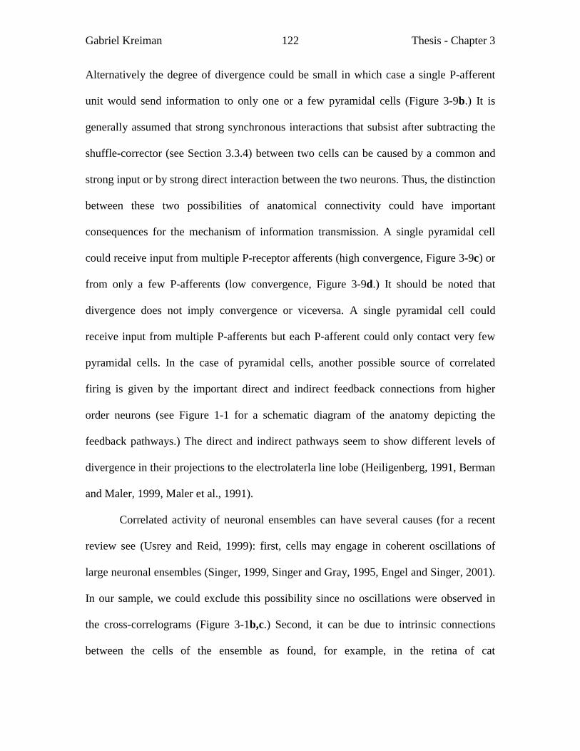
Gabriel Kreiman Thesis - Chapter 3
122
Alternatively the degree of divergence could be small in which case a single P-afferent
unit would send information to only one or a few pyramidal cells (Figure 3-9b.) It is
generally assumed that strong synchronous interactions that subsist after subtracting the
shuffle-corrector (see Section 3.3.4) between two cells can be caused by a common and
strong input or by strong direct interaction between the two neurons. Thus, the distinction
between these two possibilities of anatomical connectivity could have important
consequences for the mechanism of information transmission. A single pyramidal cell
could receive input from multiple P-receptor afferents (high convergence, Figure 3-9c) or
from only a few P-afferents (low convergence, Figure 3-9d.) It should be noted that
divergence does not imply convergence or viceversa. A single pyramidal cell could
receive input from multiple P-afferents but each P-afferent could only contact very few
pyramidal cells. In the case of pyramidal cells, another possible source of correlated
firing is given by the important direct and indirect feedback connections from higher
order neurons (see Figure 1-1 for a schematic diagram of the anatomy depicting the
feedback pathways.) The direct and indirect pathways seem to show different levels of
divergence in their projections to the electrolaterla line lobe (Heiligenberg, 1991, Berman
and Maler, 1999, Maler et al., 1991).
Correlated activity of neuronal ensembles can have several causes (for a recent
review see (Usrey and Reid, 1999): first, cells may engage in coherent oscillations of
large neuronal ensembles (Singer, 1999, Singer and Gray, 1995, Engel and Singer, 2001).
In our sample, we could exclude this possibility since no oscillations were observed in
the cross-correlograms (Figure 3-1b,c.) Second, it can be due to intrinsic connections
between the cells of the ensemble as found, for example, in the retina of cat
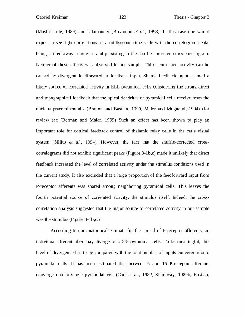
Gabriel Kreiman Thesis - Chapter 3
123
(Mastronarde, 1989) and salamander (Brivanlou et al., 1998). In this case one would
expect to see tight correlations on a millisecond time scale with the correlogram peaks
being shifted away from zero and persisting in the shuffle-corrected cross-correlogram.
Neither of these effects was observed in our sample. Third, correlated activity can be
caused by divergent feedforward or feedback input. Shared feedback input seemed a
likely source of correlated activity in ELL pyramidal cells considering the strong direct
and topographical feedback that the apical dendrites of pyramidal cells receive from the
nucleus praeeminentialis (Bratton and Bastian, 1990, Maler and Mugnaini, 1994) (for
review see (Berman and Maler, 1999) Such an effect has been shown to play an
important role for cortical feedback control of thalamic relay cells in the cat’s visual
system (Sillito et al., 1994). However, the fact that the shuffle-corrected cross-
correlograms did not exhibit significant peaks (Figure 3-1b,c) made it unlikely that direct
feedback increased the level of correlated activity under the stimulus conditions used in
the current study. It also excluded that a large proportion of the feedforward input from
P-receptor afferents was shared among neighboring pyramidal cells. This leaves the
fourth potential source of correlated activity, the stimulus itself. Indeed, the cross-
correlation analysis suggested that the major source of correlated activity in our sample
was the stimulus (Figure 3-1b,c.)
According to our anatomical estimate for the spread of P-receptor afferents, an
individual afferent fiber may diverge onto 3-8 pyramidal cells. To be meaningful, this
level of divergence has to be compared with the total number of inputs converging onto
pyramidal cells. It has been estimated that between 6 and 15 P-receptor afferents
converge onto a single pyramidal cell (Carr et al., 1982, Shumway, 1989b, Bastian,
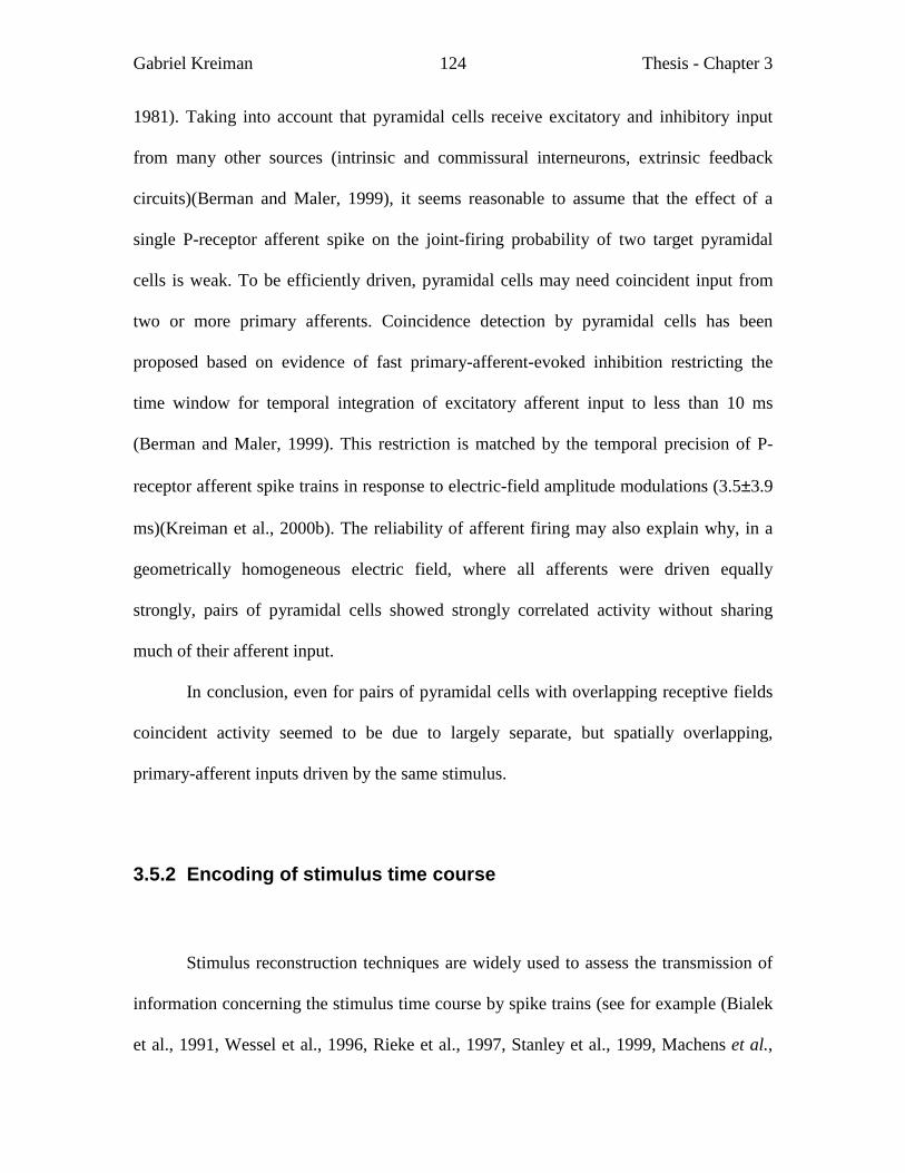
Gabriel Kreiman Thesis - Chapter 3
124
1981). Taking into account that pyramidal cells receive excitatory and inhibitory input
from many other sources (intrinsic and commissural interneurons, extrinsic feedback
circuits)(Berman and Maler, 1999), it seems reasonable to assume that the effect of a
single P-receptor afferent spike on the joint-firing probability of two target pyramidal
cells is weak. To be efficiently driven, pyramidal cells may need coincident input from
two or more primary afferents. Coincidence detection by pyramidal cells has been
proposed based on evidence of fast primary-afferent-evoked inhibition restricting the
time window for temporal integration of excitatory afferent input to less than 10 ms
(Berman and Maler, 1999). This restriction is matched by the temporal precision of P-
receptor afferent spike trains in response to electric-field amplitude modulations (3.5±3.9
ms)(Kreiman et al., 2000b). The reliability of afferent firing may also explain why, in a
geometrically homogeneous electric field, where all afferents were driven equally
strongly, pairs of pyramidal cells showed strongly correlated activity without sharing
much of their afferent input.
In conclusion, even for pairs of pyramidal cells with overlapping receptive fields
coincident activity seemed to be due to largely separate, but spatially overlapping,
primary-afferent inputs driven by the same stimulus.
3.5.2 Encoding of stimulus time course
Stimulus reconstruction techniques are widely used to assess the transmission of
information concerning the stimulus time course by spike trains (see for example (Bialek
et al., 1991, Wessel et al., 1996, Rieke et al., 1997, Stanley et al., 1999, Machens et al.,
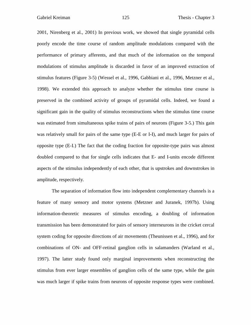
Gabriel Kreiman Thesis - Chapter 3
125
2001, Nirenberg et al., 2001) In previous work, we showed that single pyramidal cells
poorly encode the time course of random amplitude modulations compared with the
performance of primary afferents, and that much of the information on the temporal
modulations of stimulus amplitude is discarded in favor of an improved extraction of
stimulus features (Figure 3-5) (Wessel et al., 1996, Gabbiani et al., 1996, Metzner et al.,
1998). We extended this approach to analyze whether the stimulus time course is
preserved in the combined activity of groups of pyramidal cells. Indeed, we found a
significant gain in the quality of stimulus reconstructions when the stimulus time course
was estimated from simultaneous spike trains of pairs of neurons (Figure 3-5.) This gain
was relatively small for pairs of the same type (E-E or I-I), and much larger for pairs of
opposite type (E-I.) The fact that the coding fraction for opposite-type pairs was almost
doubled compared to that for single cells indicates that E- and I-units encode different
aspects of the stimulus independently of each other, that is upstrokes and downstrokes in
amplitude, respectively.
The separation of information flow into independent complementary channels is a
feature of many sensory and motor systems (Metzner and Juranek, 1997b). Using
information-theoretic measures of stimulus encoding, a doubling of information
transmission has been demonstrated for pairs of sensory interneurons in the cricket cercal
system coding for opposite directions of air movements (Theunissen et al., 1996), and for
combinations of ON- and OFF-retinal ganglion cells in salamanders (Warland et al.,
1997). The latter study found only marginal improvements when reconstructing the
stimulus from ever larger ensembles of ganglion cells of the same type, while the gain
was much larger if spike trains from neurons of opposite response types were combined.
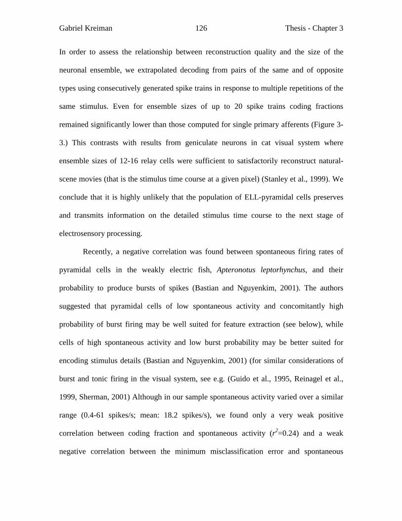
Gabriel Kreiman Thesis - Chapter 3
126
In order to assess the relationship between reconstruction quality and the size of the
neuronal ensemble, we extrapolated decoding from pairs of the same and of opposite
types using consecutively generated spike trains in response to multiple repetitions of the
same stimulus. Even for ensemble sizes of up to 20 spike trains coding fractions
remained significantly lower than those computed for single primary afferents (Figure 3-
3.) This contrasts with results from geniculate neurons in cat visual system where
ensemble sizes of 12-16 relay cells were sufficient to satisfactorily reconstruct natural-
scene movies (that is the stimulus time course at a given pixel) (Stanley et al., 1999). We
conclude that it is highly unlikely that the population of ELL-pyramidal cells preserves
and transmits information on the detailed stimulus time course to the next stage of
electrosensory processing.
Recently, a negative correlation was found between spontaneous firing rates of
pyramidal cells in the weakly electric fish, Apteronotus leptorhynchus, and their
probability to produce bursts of spikes (Bastian and Nguyenkim, 2001). The authors
suggested that pyramidal cells of low spontaneous activity and concomitantly high
probability of burst firing may be well suited for feature extraction (see below), while
cells of high spontaneous activity and low burst probability may be better suited for
encoding stimulus details (Bastian and Nguyenkim, 2001) (for similar considerations of
burst and tonic firing in the visual system, see e.g. (Guido et al., 1995, Reinagel et al.,
1999, Sherman, 2001) Although in our sample spontaneous activity varied over a similar
range (0.4-61 spikes/s; mean: 18.2 spikes/s), we found only a very weak positive
correlation between coding fraction and spontaneous activity (r2=0.24) and a weak
negative correlation between the minimum misclassification error and spontaneous
Gabriel Kreiman Thesis - Chapter 3
127
activity (r2=-0.18.) Thus, our data do not support a separation of pyramidal cells into
specialized populations. A possible cause for this difference could be that in the study of
Bastian and Nguyenkim (Bastian and Nguyenkim, 2001) a different, though closely
related species was used, and that firing rate and burst probability were determined for
spontaneous and not for stimulus-driven activity.
3.5.3 Extraction of stimulus features by “distributed bursts”
As shown previously, spikes produced by pyramidal cells reliably indicate the
presence or absence of specific stimulus features: upstrokes and downstrokes in the
amplitude of the electric field (Gabbiani et al., 1996, Metzner et al., 1998). Action
potentials occurring in short bursts perform significantly better than isolated spikes. Here,
we showed that the reliability of feature extraction further increased when the analysis
was based on spikes from a pair of neurons of the same type coinciding within a small
time window of 5-10 ms (Figures 3-5 and 3-6.) If the electrosensory system uses some
form of coincidence detection to analyze correlations between ELL-pyramidal cell spike
trains, it can only occur at the next higher-order level of electrosensory processing, that
is, the torus semicircularis of the midbrain (see Chapter 1, Figure 3-1 and (Heiligenberg,
1991). A series of studies has described the temporal filtering properties of toral neurons
for AMs of the electric field, (see for example (Rose and Fortune, 1999, Fortune and
Rose, 2000), but so far none has directly addressed feature extraction at this level of
processing or the effect of coincident input from ELL-pyramidal cells.
Gabriel Kreiman Thesis - Chapter 3
128
Bursts and synchronous activity by thalamic relay cells in the visual system have
attracted much attention in recent years. It has been shown that geniculate cells can
switch between two modes of firing, tonic and burst (for review see (Sherman, 2001)
Since bursts as well as spikes generated in tonic mode encode visual information, it was
suggested that bursts signal the detection of objects to the cortex while tonic firing may
serve in the encoding of object details (Guido et al., 1995, Reinagel et al., 1999, Sherman,
2001). Interestingly, both bursts of single cells and coincident spikes fired by two relay
cells with overlapping receptive fields are able to efficiently drive layer IV simple cells
(Alonso et al., 1996, Usrey et al., 2000, Usrey and Reid, 1999). Both mechanisms have
been suggested to make information transmission to the cortex more reliable. In addition
to just “getting the signal through” to the cortex, coincident activity may also contain
improved spatial information. Enhanced spatial resolution has been demonstrated for the
coincident activity of pairs of visual cortical cells in cat with overlapping receptive fields
(Ghose et al., 1994), and has also been suggested for concerted firing patterns among
salamander retinal ganglion cells (Meister, 1996, Meister et al., 1995). It has been shown
for geniculate neurons in cat (Dan et al., 1998) and for retinal ganglion cells in
salamander (Meister et al., 1995) that temporally correlated activity could even be used
as an additional and channel of information flow to the cortex. Similarly, it is possible
that correlated activity may improve spatial information in weakly electric fish, since the
activity of two pyramidal cells with overlapping receptive fields will only then be
correlated when both receptive fields are affected by the same stimulus. To quantify the
gain in spatial information as well as in feature-extraction reliability, experiments are
Gabriel Kreiman Thesis - Chapter 3
129
needed involving objects being moved across the overlapping receptive fields of two
simultaneously recorded pyramidal cells.
The time scales determined for interspike intervals within bursts of single neurons
were approximately 7-15 ms (Gabbiani et al., 1996, Metzner et al., 1998). The time scales
estimated for the optimal coincidence time window for feature extraction were
approximately 5-10 ms (see Figure 3-5). It is interesting to note that these values are
remarkably similar. This suggests that integration of both burst-like spike patterns
arriving on single neurons and coincident spikes on groups of pyramidal cells may
contribute to the detection of stimulus features. Therefore, temporally correlated activity
of groups of pyramidal cells may be considered to represent a form of “distributed
bursts“. It has even been suggested that coincident bursts of spikes may constitute the
“best neural code” used for synaptic transmission and information coding (Lisman,
1997). Indeed, our data support this notion since a large percentage of the coincident
spikes occurred in bursts (63±15%, mean ± s.d. for a coincidence window of ±5 ms; see
Figure 3-4c.) Studying postsynaptic effects of pyramidal-cell spike patterns on their
target neurons in the midbrain torus will help to elucidate the physiological significance
of such distributed bursts.

Gabriel Kreiman Thesis - Chapter 3
130
3.6 Figure legends
Figure 3-1 Correlated activity of simultaneously recorded pyramidal cells
(a) Representative raster plot segments of the spike trains of 2 simultaneously recorded I-
units with overlapping receptive fields. The top trace shows the time course of the
random amplitude modulation (cutoff frequency fc = 10 Hz, contrast 25%.) Action
potentials occurring within a burst of spikes are indicated by a thick line. The same
stimulus was repeated 5 times yielding 5 raster lines for each neuron. (b) Cross-
correlograms of the responses of the two I-units computed with a bin size of 3 ms. The x-
axis indicates the time lag between the coincident spikes. The y-axis shows the number of
coincident spikes per second (that is, the number of coincidences in each 3 ms bin was
normalized to indicate the coincidences/sec). The strong peak centered at 6.3 ms indicates
that these two I-units fired coincident spikes within small time windows. The horizontal
dashed line gives the expected value for two homogeneous Poisson neurons of the same
firing rates as the recorded units firing independently. The peak and width (37 ms) of the
responses are marked by vertical and horizontal arrows, respectively. Inset: the shuffle-
corrected cross-correlogram. The horizontal line at 0 indicates the expected value for
independent responses and the dashed lines show the 2σ-confidence limits under this null
hypothesis (see Methods.) Since the solid curve fell between these bounds, we conclude
that the synchrony is mainly stimulus-induced. The average firing rates for the two units
were 9.4 and 15.2 spikes/s, respectively. (c) Cross-correlogram of the responses of one E-
and one I-unit. The central trough shows that these cells of opposing response type fired
in anticorrelation. The minimum occurred at -0.2 ms, the width at half-height was 10 ms.
Gabriel Kreiman Thesis - Chapter 3
131
Inset: the shuffle-corrected cross-correlogram. The average firing rates for the two units
were 17.3 and 12.3 spikes/s, respectively.
Figure 3-2 Properties of the cross-correlograms for pairs of units of the same type
For each neuronal pair, values for 5 stimulus contrasts are included (n=16; fc=5Hz.) (a)
Distribution of the times at which the maximum occurred. Bin size = 5 ms. (b)
Distribution of the maxima of the cross-correlograms. Bin size = 0.25 coincidences/s.
The x-axis was cut at 5 coincidences/s for clarity; there were 3 values beyond the axis
limit (at 7.2, 9.3, and 19.1 coincidences/s.) (c) Distribution of the widths at half-height of
the peaks. Bin size = 25 ms. Arrows indicate mean values.
Figure 3-3 Summarized results of stimulus estimation
Summarized results of stimulus estimation from spike trains of P-receptor afferents,
single pyramidal cells, and pairs of simultaneously recorded pyramidal cells of the same
type (E-E and I-I) and of opposite type (E-I) (fc=5 Hz.) The accuracy of the information
transmitted about the time course of a stimulus is characterized by the coding fraction.
Error bars represent standard deviations. n: overall number of experimental conditions
(contrasts) for all cells or cell pairs analyzed . Data for P-receptor afferents taken from
(Kreiman et al., 2000b).
Figure 3-4 Euclidian features and coincident spikes
Euclidian features and coincident spikes for the pair of I-type pyramidal cells depicted in
Figure 3-1. (a) Euclidian feature for each of the two cells. (b) Raster plot example
Gabriel Kreiman Thesis - Chapter 3
132
highlighting those spikes which occur synchronously within a time window of ±5 ms as
thick bars. (c) The proportion of coincident spikes with respect to the total number of
spikes for neuron A (top) and neuron B (bottom) is shown as black bars as a function of
the size of the coincidence window. The percentage of spikes that occur in bursts and
coincide are shown as white bars. The overall percentage of bursting spikes is indicated
as a gray bar at right.
Figure 3-5 Feature extraction for pyramidal cell pairs
Feature extraction by the same pair of I-type pyramidal cells illustrated in Figure 3-1. (a)
Minimum probability of misclassification, pE, by those spikes of neurons A and B,
respectively, which had a coincident spike on the respective other neuron plotted against
the size of the coincidence time window. pE is the average of two error probablities: in
case of this I-unit pair, these are the probability that coincident spikes are fired even when
there is no downstroke in stimulus amplitude (false alarms) and the probability that a
downstroke occurs but fails to elicit coincident spikes (misses.) pE decreased with
decreasing size of the coincidence time window, indicating that spikes coinciding within
a time window of ±5 ms transmit the information on the occurrence of stimulus features
more reliably than spikes of single neurons. Filled symbols: neuron A; open symbols:
neuron B. (b) Single-neuron performance of unit A and B, respectively.
Figure 3-6 Summary diagram of feature extraction performance by ELL pyramidal cells.
From left to right, bars indicate the average pE for coincident spikes of E-E pairs and I-I
pairs, for coincident spikes of E-E and I-I pairs after shuffling of trials, for spike bursts of
Gabriel Kreiman Thesis - Chapter 3
133
single E- and single I-units, for isolated spikes of single E-units and single I-units, and for
coincident spikes of E-I pairs before and after shuffling of trials. Single I-units and pairs
of I-units performed better than single E-units and pairs of E-units, respectively (p<0.5
and p<0.01, respectively; 2-tailed t- test.) Pairs of cells of the same type performed better
than bursts of spikes of single pyramidal cells (p<0.01 for both, E- and I-type neurons),
which, in turn, performed better than isolated spikes fired by the respective units (p<0.01
for both, E- and I-type neurons.) Feature extraction by opposite-type pairs was close to
chance performance (pE = 0.5.) pE computed for shuffled spike trains was not
significantly different from pE calculated for simultaneously recorded spike trains. The
mean values of pE were computed from the lowest values of pE observed irrespective of
the size of the best time window. Time windows smaller than 5 ms were not used because
the number of spikes coinciding within such a time frame was too small to yield reliable
results (see Figure 3-4c.) Error bars represent standard errors of the mean. The numbers
below the bars give the overall number of stimulus conditions (cutoff frequencies and
contrasts) for all cells or cell pairs analyzed.
Figure 3-7 Terminal spread of P-receptor afferents
Top: Transverse sections at hindbrain level in two preparations (left and right,
respectively.) The locations of the terminal fields of two Neurobiotin-filled P-receptor
afferent fibers within CM are indicated by the boxes. Bottom: Magnified views of the
respective cells. In both cases the terminal fields were reconstructed from 3 consecutive
transverse sections (thickness: 50 µm) of the ELL. Section at left corresponds to level -6,
and section at right to level -9 of the brain atlas of Maler et al.(Maler et al., 1991). C:
Gabriel Kreiman Thesis - Chapter 3
134
Cerebello-medullary cistern; CCb: Corpus Cerebelli; CM: Centro-Medial segment of
ELL; CL: Centro-Lateral segment of ELL; d: dorsal; g: granular cell layer of ELL; l:
lateral; L: Lateral segment of ELL; M: Medial segment of ELL; MLF: Medial
Longitudinal Fasciculus.
Figure 3-8: Spontaneous activity of pyramidal cells
Distribution of the spontaneous firing rates of the pyramidal cell units that were studied
in this Chapter. The spontaneous activity was recorded during a 30 second period before
the presentation of RAM stimulus, in this case under an unmodulated carrier signal (that
is, using the mimic of the fish's own EOD without any amplitude modulation, see
Chapter 1). In several of the experiments, a 30 second period without RAM or sinusoidal
modulation was also interspersed within the experiment. The arrow indicates the mean
value. Bin size = 2 spikes/sec. E-type and I-type pyramidal cells were pooled in this
figure; no significant differences in the spontaneous activity were observed between the
two groups.
Figure 3-9: Schematic of different anatomical configurations for the P-receptor to ELL
projection
This schematic diagram illustrates different possibilities for the convergence and
divergence of projections of connectivity from the P-receptor afferent units to the E-type
pyramidal cells in the ELL. (a) High divergence condition where a single P-receptor
afferent unit synapses directly onto a large number of E-type pyramidal cells. (b) Low
divergence situation where a single P-unit is connected to only very few pyramidal cells.

Gabriel Kreiman Thesis - Chapter 3
135
In the scheme a one-to-one connection is depicted but the conclusions described in the
text also apply for a sparse connectivity that is not one-to-one. Furthermore, it is
important to emphasize that low divergence does not imply low convergence. In this
scheme a single pyramidal cell is shown to receive input from a single P-receptor afferent
but it would be easy to depict a low divergence with high convergence situation. (c) High
convergence situation where multiple P-receptors send information to the same pyramidal
cell. (d) Low convergence situation where each pyramidal cell only receives information
from one or very few P-receptor afferent units.
Figure 3-10: Change in correlogram properties with the stimulus bandwidth
Change in correlogram properties with stimulus bandwidth for the pair illustrated in
Figure 3-1. (a) The peak value of the correlogram increased with stimulus bandwidth.
Each point corresponds to a separate stimulus condition (fc or contrast.) The dashed line
indicates a linear fit to the data (slope = 0.06 coincidences/(sec.Hz), r2 = 0.97.) (b) The
width at half height decreased with increasing stimulus bandwidth. Each point
corresponds to a separate stimulus condition. The dashed line indicates a linear fit to the
data (slope = -6.8 ms/Hz, r2 = -0.72.) (c) There was no clear correlation between the time
at which the peak occurred and the bandwidth of the stimulus. Each point corresponds to
a separate stimulus condition. The dashed line indicates a linear fit to the data (slope =
0.36 ms/Hz, r2 = 0.26.)

Gabriel Kreiman Thesis - Chapter 3
136
Figure 3-1

Gabriel Kreiman Thesis - Chapter 3
137
Figure 3-2

Gabriel Kreiman Thesis - Chapter 3
138
Figure 3-3

Gabriel Kreiman Thesis - Chapter 3
139
Figure 3-4

Gabriel Kreiman Thesis - Chapter 3
140
Figure 3-5

Gabriel Kreiman Thesis - Chapter 3
141
Figure 3-6

Gabriel Kreiman Thesis - Chapter 3
142
Figure 3-7

Gabriel Kreiman Thesis - Chapter 3
143
Figure 3-8

Gabriel Kreiman Thesis - Chapter 3
144
Figure 3-9

Gabriel Kreiman Thesis - Chapter 3
145
Figure 3-10

Gabriel Kreiman Thesis - Chapter 4
146
4 In search of attentional modulation in the ELL19
4.1 Scope and motivation of the project
Selective attention plays a fundamental role in the processing and gating of
information in the nervous system. This has been most thoroughly explored in the visual
system where it has been shown that paying attention can modulate the neuronal activity
in different areas in monkeys and humans (O'Craven et al., 1997, McAdams and
Maunsell, 1999, Steinmetz et al., 2000, Desimone and Duncan, 1995, Fries et al., 2001,
Maunsell, 1995) Attention has been shown to alter the blood flow as measured in
functional imaging experiments, the neuronal firing rates, neuronal reliability and
neuronal synchrony.
The electric fish offers an ideal model system to explore the potential role of
attention in the processing of sensory information. The gating of information from the P-
receptor afferents to the ELL to higher structures like the Torus Semicircularis might be
influenced by the behavioral significance of the stimuli or the saliency of a stimulus with
respect to the background information. Pyramidal cells receive massive efferent feedback
projections, both excitatory and inhibitory, from higher order electrosensory structures
19 A warning to the reader: At the time of writing this Thesis, the preliminary observations that we have drawn from the work described in the current Chapter do not seem to yield the fascinating results that we had expected. Therefore, these data have not been published and the reader might decide not to engage in examining several pages that are not (yet) conclusive. However, as Nobel Prize winner Luis Federico Leloir used to say: "The most important and fascinating experiments are those that end up in the sink" (my translation.)
Gabriel Kreiman Thesis - Chapter 4
147
that terminate primarily on their large apical dendrites (see schematic diagram in Chapter
1, Figure 1 and (Carr et al., 1986, Maler and Mugnaini, 1994) The extensive inhibitory
feedback was suggested to play a role in adaptive gain control and a "searchlight"
mechanism that would allow the animal to increase the detectability of scanned objects
(Crick, 1984, Bratton and Bastian, 1990, Maler and Mugnaini, 1994, Berman and Maler,
1999) This putative searchlight mechanism could play an important role in the detection
of novel stimuli positioned within the receptive field of pyramidal cells. The direct
feedback pathway to the ELL has many of the characteristics that were suggested by
Crick to play an important role in sensory "searchlight" mechanism (Crick, 1984): (i) A
positive feedback loop is formed by a subset of the ELL / nucleus praeminentialis
dorsalis feedback and feedforward projections. These projections are reciprocal,
topographic and excitatory. (ii) The nucleus praeminentialis neurons show larger
receptive fields than those of neurons in the ELL. (iii) the inhibitory direct feedback
pathway from the nucleus praeminentialis is topographically diffuse. Furthermore, Crick
suggested that a non-linearity would be required to amplify signals in a searchlight
mechanism. Maler and colleagues have suggested that the several types of non-linear
elements occur in the ELL that would be ideally suited for this purpose: (i) voltage-
dependent EPSPs, (ii) Dendritic spike bursts, (iii) voltage-dependent inhibition and (iv)
frequency-dependent synaptic facilitation (Berman and Maler, 1999). We therefore set to
attempt to directly evaluate this possibility at the electrophysiological level.
Gabriel Kreiman Thesis - Chapter 4
148
4.2 Methodological procedures
4.2.1 Stimulation
As in the previous Chapters, all the experimental work was carried out by Rüdiger
Krahe and Walter Metzner at the University of California at Riverside20. All the
experiments described in the previous Chapters were performed by using a global
stimulation elicited by electrodes in or near the mouth and tail of the animal21 (see
Chapter 1.) Here we also mapped the cells' receptive fields by using a localized dipole
stimulus moved along the body of the animal. The responses were tested as described in
the previous Chapters. In addition to the wide-band RAMs, we also used stimuli that
were band-pass filtered (5-10 Hz; 10-20 Hz and 20-40 Hz.)22 Performance in stimulus
reconstruction can be easily compared to the ones with wide-band stimulation by
integrating the signal-to-noise ratio over the corresponding frequency bands (see Chapter
1 and (Gabbiani and Koch, 1998)). Thus, when analyzing the responses to band-pass
stimuli, we computed signal-to-noise ratios for stimulus estimation (or equivalently
coherence functions) in the frequency domain to quantify the responses of pyramidal
cells. Whole-body stimuli were presented by modulation of the electric field between the
mouth and tail of the fish as described in Chapter 1 (see also (Wessel et al., 1996,
20 Currently at the University of California at Los Angeles. 21 The animal was paralyzed but not anesthetized as in all our previous experiments. To what extent this could play a role in the type of responses that we have observed is still unclear. It should be noted that at least with the current experimental setup, paralyzing the animal is necessary for performing the electrophysiological recordings. 22 Band-pass white noise stimuli were generated as described before by first generating a white noise signal and then filtering the corresponding frequency bands using a 4-pole Butterworth filter in MATLAB.
Gabriel Kreiman Thesis - Chapter 4
149
Kreiman et al., 2000b, Metzner et al., 1998) Localized stimuli consisted of the same
RAMs used for whole-body stimuli, but were presented using a moveable electrode
positioned < 1 cm from the skin surface within the receptive field of the recorded units
(reference electrode remains in mouth.) Initially, we used whole-body stimulation with
sinusoidal AMs to obtain a stable recording. Subsequently, localized stimulation with
sinusoidal AMs was used to determine which body surface area resulted in an optimal
response (audio-visual monitoring of recording.)23 The electrode consisted of a chloride
silver wire within a hand-held, fire-polished glass pipette of 1 mm diameter (see
(Shumway, 1989a) Localized RAMs was presented through another localized electrode
attached to a micromanipulator and positioned in the same area on the surface of the skin.
In addition, a constant background electric field without RAMs was generated by whole-
body stimulation. Although different experimental protocols were tested, in the most
general case, a global RAM stimulus was presented for a duration of 30 seconds. During
the first 15 seconds, only the global stimulation was presented. During the last 15 seconds
the local stimulation was presented on top of the global stimulus. In other experiments,
the global and local stimuli were presented separately. While the results in Chapter 3
showed that multiple spike trains from pyramidal cells do not carry detailed time-course
information under conditions of global stimulation, as used in the previous single cell
studies (Gabbiani et al., 1996, Metzner et al., 1998), it is however conceivable that
pyramidal cells might convey such information in response to localized stimuli or under
conditions mimicking attentionally salient stimuli.
23 The sinusoidal stimuli were used only for establishing a stable recording and for coarse mapping of the receptive fields. All the data analysis described in the current Chapter was performed with the RAM stimuli (either from 0 up to a given fc or band-pass stimuli as described above).

Gabriel Kreiman Thesis - Chapter 4
150
4.2.2 Electrophysiology
The procedures for electrophysiological recordings were described in Chapter 1
and some specific details about the recordings from pyramidal cells in the ELL were
described in Chapter 3.
4.2.3 Data analysis
We compared the responses of pyramidal cells to localized stimulation with the
responses of pyramidal cells stimulated only by the whole-body (global) stimulus and
with local stimulus superimposed on the global one. The computational techniques for
stimulus reconstruction and feature extraction were described in Chapter 1. The-60
seconds stimulation time was subdivided into several different segments for analysis. In
particular we were interested in comparing the initial 30 seconds where only global
stimulation was applied, the initial phase of the combined local and global stimulation
and the neuronal activity to the combined stimulus after the initial possibly transient
response. This is further described in Section 4.3 below.
4.3 Preliminary results
Mapping the receptive fields of the recorded neurons (see Figure 4-1) allowed us
to deliver local stimulation in contrast to the whole-body stimulation procedure utilized in
the previous work (see Chapters 2, 3 and (Kreiman et al., 2000b, Wessel et al., 1996,

Gabriel Kreiman Thesis - Chapter 4
151
Gabbiani et al., 1996, Metzner et al., 1998) While we tried a number of different ways of
presenting the stimulus, the most typical situation is depicted in Figure 4-2.
4.3.1 Neuronal response, example
First, there was a period of 30 seconds where only global stimulation was applied
(Figure 4-2a.) At t = 30 seconds, the global stimulus remained on while a local stimulus
was delivered through the electrode position within the neuron's receptive field (Figure
4-2b.) The raster plot does not show any clear indication of changes in the neuronal
activity upon turning on the local stimulation. The last part of the figure illustrates a later
portion of the local stimulation superimposed on the global stimulus which lasted for 30
seconds (Figure 4-2c.) The neuron fires near the peaks of the global stimulus in Figure
4-2a. During the combined local and global stimulation it seems that the neuron would
still respond to several of the peaks in the global stimulus but not as strongly and reliably
as before. In particular, it seems to respond to the troughs in the local stimulus and a
strong burst of activity seems to occur when there is a close temporal occurrence of peaks
in the global stimulus and troughs in the local stimulus (Figure 4-2b-c.)
This was confirmed by computing the Euclidian classifiers as described in
Chapter 1 independently for the global and local stimulus Figure 4-3b-e. The Euclidian
feature computed from the global stimulus was an upstroke in the electric field amplitude
both when the global stimulus was presented alone (Figure 4-3b) or in the presence of the
local stimulus (Figure 4-3c.) For the local stimulus, the Euclidian feature showed a
downstroke in the amplitude (Figure 4-3d.) This Euclidian feature was similar in the
initial phase of the local stimulus or during the later portion of the experiment (Figure

Gabriel Kreiman Thesis - Chapter 4
152
4-3e.) We quantified the performance of isolated spikes and bursts of spikes in extracting
upstrokes and downstrokes by computing the probability of misclassification, pe, during
different intervals in the experiment (Figure 4-3f.) As discussed previously (see Chapter
1 and (Gabbiani et al., 1996, Metzner et al., 1998) bursts of spikes yielded a lower value
of pe than isolated spikes. No statistically significant differences were observed among
the values of pe computed from the global stimulus in the whole experiment (wg), global
stimulus alone (g1), global stimulus in the presence of local stimulation (g2), local
stimulus in the whole experiment (wl), initial local stimulus presentation (l1) or last
portion of the local stimulus presentation (l2) (one-way ANOVA, p > 0.3 for isolated
spikes and p > 0.2 for burst of spikes.) We did not observe a significant change in the
firing rate computed in different time windows of at least 1000 ms duration within the
experiment (see Figure 4-3g.)
It is possible that the global versus local stimulation could be accompanied not by
a change in feature extraction performance or the firing rate but an alteration in the
reliability of the neuronal responses. The appearance of a sudden salient local stimulus in
the neuron's receptive field could be correlated with a sharp burst of activity with a
precise latency. To address this issue, we used the Victor-Purpura distances between
spike trains as a measure of the trial-to-trial variability in the neuronal response (see
Chapter 2 for details about this metric.) The mean normalized distances between
successive repetitions of the identical stimulus are illustrated in Figure 4-4 for three
different values of the spike moving cost parameter, q. No significant differences were
observed in the different intervals that were analyzed (see Figure 4-4 for details) at any of
Gabriel Kreiman Thesis - Chapter 4
153
the values of q. Thus, there does not seem to be a change in the reliability of the neuronal
response with the appearance of a sudden local stimulus.
4.3.2 Summary of results
A summary of the changes in firing rate for the 96 experiments from recordings in
24 pyramidal cells that were recorded in this particular paradigm is presented in Figure
4-5. An average of the absolute values of the firing rate during eight relevant different
time intervals is depicted in Figure 4-5b. The average of the absolute firing rates could
preclude from observing real differences that could be hidden in the changes in
spontaneous activity of the neurons. Therefore, Figure 4-5a shows the mean firing rates
normalized by the mean firing rate of the neuron24. There were no significant differences
in the firing rates among the different time intervals (one-way ANOVA, p > 0.25.)
The average performance of the pyramidal neurons in the feature extraction task
during the different intervals is shown in Figure 4-6. There was no significant difference
in the probability of misclassification by the Euclidian feature among the global
stimulation alone or the global stimulation in the presence of local stimulation. There was
also no statistically significant difference between the period at the onset of the local
stimulation period and the later period of local stimulation.
Finally, the average normalized distances between spike trains are shown in
Figure 4-7. We did not observe a statistically significant difference among the different
periods of analysis in the trial-to-trial reliability of the neuronal responses.
24 The mean firing rate was computed over the whole experimental session. Similar results were obtained when using the spontaneous activity for the normalization.
Gabriel Kreiman Thesis - Chapter 4
154
4.4 Feature extraction by E vs. I type pyramidal cells under
different stimulation conditions
As reported previously (Gabbiani and Metzner, 1999, Gabbiani et al., 1996,
Metzner et al., 1998), we observed a small but significant difference in the performance
of E- and I-type pyramidal cells in the feature extraction task (see Chapter 3). In general,
I units showed smaller values of probability of misclassification than E units. This
difference was hypothesized to be due to differences in connectivity between the two
types of pyramidal cells: E-units receive direct inhibitory input from ovoid cells while I-
units do not. Ovoid cells have large dendritic fields (Bastian et al., 1993). This suggests
that they probably have very broad receptive fields. Furthermore, ovoid cells show
extensive axon-terminal fields both ipsilateral and contralateral to their dendrites (Bastian
et al., 1993). This inhibitory input is thought to serve in common-mode rejection: global
amplitude modulation of the electric field (in an "identical-geometry" field stimulation
paradigm, (Heiligenberg, 1991, Heiligenberg and Bastian, 1984)) would maximally
stimulate ovoid cells on both sides of the brain in phase with the E-units. There, the
responses of E-type pyramidal cells would be down regulated by inhibition from ovoid
cells. Potentially, I-units may be affected, too, but only indirectly via granule cells. We
therefore decided to study how the difference in the probability of misclassification
between E- and I-units is affected by the characteristics of the stimulation. In particular,
we directly addressed the above hypothesis that would predict that the difference between
E and I pyramidal cells disappears or decreases when common-mode rejection is
minimized. The experimental procedures described earlier in this Chapter to investigate
the putative modulation of neuronal responses by salient stimuli could be directly applied

Gabriel Kreiman Thesis - Chapter 4
155
to answer this question. We compared the performance of E and I units under conditions
in which the ovoid cells would presumably be only weakly stimulated. The weakest input
to ovoid cells should occur for highly localized stimuli when only a small part of the
receptive field is subject to amplitude modulation in the electric field. We recorded the
activity of individual pyramidal cells under global and local stimulation.
Preliminary results from this study are shown in Figure 4-8. We recorded the
activity of 27 pyramidal neurons (we analyzed the responses of 24 neurons, 15 I units, 9
E units, the remaining 3 showed low quality firing) under global and local random
amplitude modulation. For each experiment, we evaluated the performance of the unit in
extracting upstrokes (E cells) and downstrokes (I cells) as described previously (see
Chapter 3). Our preliminary observations suggest that the difference in feature extraction
between E and I type pyramidal cells (Figure 4-8a) disappears under conditions of local
stimulation (Figure 4-9b). This suggests that E and I type pyramidal neurons show
differential processing of the incoming signal; this may be due to the different anatomical
input provided by the ovoid cells as discussed in the previous paragraph.
4.5 Discussion
We did not observe any clear differences in the neuronal responses during our
preliminary explorations of the possible effects of local stimulation. Electric fish show a
remarkable capacity to detect small objects in the environment by using the alterations in
the electric field (Nelson and Maciver, 1999) Thus, it seems that a salient stimulus should
elicit a strong and reliable signal.
Gabriel Kreiman Thesis - Chapter 4
156
Perhaps the local stimulation that we have presented did not constitute a salient
stimulus. While it was verified that the neuron's activity was modulated in the presence of
the local stimulus alone25, it is not entirely clear what the effective stimulus in the skin of
the fish was. The transdermal potential across the skin is proportional to some weighted
sum of the global plus local stimulation. But this is too vague for a rigorous quantitative
analysis. Since we did not measure the transdermal potential (nor the electric field
directly near the skin), it is unclear what those weights were during the combined
stimulation. This could be quite important in understanding the efficiency of the local
stimulus in generating a salient response.
It is possible that the fact that the animal was paralyzed could be related to the
lack of attentional gating responses. It is unclear how to verify this assertion given that, at
least with the current recording technology, protocols and paradigm, this is a necessary
part of the electrophysiological preparation procedure. It should be noted that the animal
was not anesthetized but only paralyzed (see Section 4.2). In attempting to draw a
comparison with the visual system, it seems unlikely that the neuronal responses in early
visual areas (such as the lateral geniculate nucleus or primary visual cortex) could be
significantly affected by paralyzing the animal. In fact, anesthesia which has a much
larger impact on the overall chemistry of the brain, only seems to have an impact in
higher visual areas. However, this is a point that should be kept in mind in interpreting
the results here described.
25 This was actually the way we used to define that the local stimulus was presented within the neuron's receptive field (see Methods in Section 4.2). In some cases, we also computed the probability of misclassification for random amplitude modulation stimulus presented locally; the pe values in those cases were clearly much better than chance levels and were comparable to those obtained with global stimulation alone (see also Figure 4-3).
Gabriel Kreiman Thesis - Chapter 4
157
It is also conceivable that the modulation of neuronal responses in the presence of
a salient stimulus is modified at a later stage in the processing of information in the
nervous system. Within the visual modality, the effects of attention are easier to find in
later extrastriate visual areas than in the earlier areas (O'Craven et al., 1997, Steinmetz et
al., 2000, Desimone and Duncan, 1995, Kanwisher and Wojciulik, 2000, Maunsell, 1995,
Logothetis, 1998). While electrophysiological effects of attention have been shown in
extrastriate visual areas, the effects seem to be very small in V1 and virtually absent in
the responses of neurons in the lateral geniculate nucleus. The electrolateral line lobe
constitutes the second stage of processing of changes in electric field amplitude
information in the electric fish. The information from the ELL is conveyed to the Torus
Semicircularis (TS.) The TS already combines information from the amplitude and phase
sensitive pathways. Our initial speculation was that the effects of attention and feedback
would be evident before the merging of amplitude and phase information but maybe this
is not the case.
It is also possible that the changes elicited by the presence of a salient stimulus
within the receptive field are evident at a level beyond the activity of a single neuron. For
example, we showed in the previous Chapter that the coincident activity of two pyramidal
cells could significantly enhance the extraction of behaviorally relevant features from the
environment. Thus, it is possible that the local stimulation could change the degree of
synchrony between multiple neurons without significantly altering their individual
responses.
Gabriel Kreiman Thesis - Chapter 4
158
While the preliminary results presented in the current Chapter do not point to a
clear difference in the responses of individual pyramidal cells, there is still much more to
explore to understand the possible mechanisms of gating of neuronal information.

Gabriel Kreiman Thesis - Chapter 4
159
4.6 Figure legends
Figure 4-1: Schematic of stimulation procedure
Schematic diagram indicating the position of the electrodes for whole body (global)
stimulation (in or near fish's mouth and tail, see Chapter 1) and those for local stimulation
(depicted by crosses here.) around an outline of the Eigenmannia electric fish. Local
electrodes were less than 1 mm away from the skin of the fish.
Figure 4-2: Pyramidal neuron activity, raster plot example
Sample of the activity of a pyramidal neuron during three 1.5-second duration epochs of
the experiment. The first epoch (a) shows the response during the initial period where
only global stimulation (dashed line) was performed. The second epoch (b) indicates the
neuronal response during the initial part of the local (continuous line) superimposed on
global stimulation (dashed line.) The last epoch (c) depicts the responses during the latest
part of the simultaneous global and local stimulation. Each tick corresponds to an action
potential and there were 5 subsequent repetitions of identical stimuli.
Figure 4-3: Example of global versus local stimulation
(a) Sample activity during a period of 5 seconds where local stimulation (gray continuous
line) was superimposed on global stimulation (black continuous line.) (b-e) Euclidian
feature classifier (see Chapter 1 for details) for isolated spikes (dashed lines) and bursts
of spikes (continuous lines) for global stimulation (black, b-c) and local stimulation

Gabriel Kreiman Thesis - Chapter 4
160
(gray, d-e.) The Euclidian feature was computed in 15 second periods as indicated at the
top of each plot: [0;15], [30;45], [30;45] and [45;60] seconds for b through d
respectively. (f) Probability of misclassification, pe, for isolated spikes (left) and bursts of
spikes (right.) The periods over which pe was computed correspond to the ones in b-d,
except for wg which indicates whole global stimulus ([0;60] seconds) and wl which
indicates whole local stimulus ([30;60 seconds.) See text for details. (g) Mean firing rates
computed over the time intervals indicated in the abscissa. Black bars indicate values for
global stimulation, grey bars indicate local stimulation.
Figure 4-4: Pyramidal neuronal trial-to-trial firing variability
The trial-to-trial variability of the responses of pyramidal cells upon repeated
presentations (n=5) of identical stimuli were evaluated by using the Victor-Purpura
distance between spike trains (see Chapter 2 and (Victor and Purpura, 1997) Here we
show the normalized spike distances in different intervals of the experiment for three
different values of the spike moving cost parameter: (a) q = 0, (b) q = 0.05, (c) q = 0.25.
The spike distances were normalized by the value of d(q→∞) (see Chapter 2 for details.)
The different bars correspond to the following time intervals (from left to right): [0;5],
[10;15], [20;25], [30;35], [40;45] and [50;55] seconds with respect to the stimulus onset.
The first three intervals were within a period of global stimulation only while during the
last three epochs, the local stimulation was superimposed on the global ones (see Section
4.2.1.)
Figure 4-5: Changes in firing rate, summary
Gabriel Kreiman Thesis - Chapter 4
161
Summary of changes in firing rate during different epochs of the experiment. (a) Mean
normalized firing rates for all (n = 96) experiments. The neuronal firing rate is
normalized by the mean spontaneous activity of the unit. The time intervals correspond to
(from left to right): [0;30], [30;40], [30;31], [31;32], [32;33], [33;34], [34;35], [40;60]
seconds with respect to global stimulation onset. (b) Mean absolute firing rates in the
same intervals. (c) Mean firing rate after subtraction of the mean activity.
Figure 4-6: Changes in probability of misclassification, summary
Summary of changes in the probability of misclassification, pe, during different epochs of
the experiment. Mean normalized values of pe for all experiments (n = 96.) The time
intervals for the analyses correspond to the ones described in Figure 4-3.
Figure 4-7: Changes in neuronal response variability, summary
Summary of changes in the trial-to-trial variability as assessed by the mean normalized
Victor-Purpura spike distances, < dn >, during different epochs of the experiment. Mean
normalized values of < dn > for all experiments (n = 96.) The time intervals for the
analyses are indicated in the abscissa.
Figure 4-8: Comparison of E versus I pyramidal cells under different stimulation conditions
Distribution of the probability of misclassification (pe, see Chapter 3) for extracting
upstrokes (E-cells, black) and downstrokes (I cells, white) in the random amplitude
modulation of the electric field. Recordings were performed under global (a) or local (b)
stimulation conditions (see Section 4.2.1 for methodological procedures). Local random
Gabriel Kreiman Thesis - Chapter 4
162
amplitude modulation was done under constant mean amplitude conditions. Bin size =
0.02. The values of pe illustrated here correspond to the probability of misclassification
for bursts of spikes. For all the data shown here, fc = 5 Hz.

Gabriel Kreiman Thesis - Chapter 4
163
Figure 4-1

Gabriel Kreiman Thesis - Chapter 4
164
Figure 4-2

Gabriel Kreiman Thesis - Chapter 4
165
Figure 4-3

Gabriel Kreiman Thesis - Chapter 4
166
Figure 4-4

Gabriel Kreiman Thesis - Chapter 4
167
Figure 4-5

Gabriel Kreiman Thesis - Chapter 4
168
Figure 4-6

Gabriel Kreiman Thesis - Chapter 4
169
Figure 4-7

Gabriel Kreiman Thesis - Chapter 4
170
Figure 4-8
Gabriel Kreiman Thesis - Chapter 5
171
171
5 Conclusions and future directions
5.1 Neural coding and feature extraction
5.1.1 Coding principles
The general question of exploring how neurons and groups of neurons encode
information has gained significant momentum in the last few years (see for example
(Roddey and Jacobs, 1996, Warland et al., 1997, Richmond et al., 1990, Shadlen and
Newsome, 1994, Warzecha et al., 1998, Shadlen and Newsome, 1998, Dan et al., 1998,
Gabbiani and Koch, 1998, Rieke et al., 1997, Bair, 1999, Reich et al., 1997, Bialek et al.,
1991, Koch and Laurent, 1999, Hatsopoulos et al., 1995, Laurent, 1996, Laurent et al.,
1996)). Neuroscientists have traveled some way from the influential work of Perkel and
Bullock (Perkel and Bullock, 1968), yet there are numerous questions that still remain
largely unclear. Perhaps one important general conclusion from the study of codes in
general, which was already hinted at in the seminal work of 1968, is that it is not
necessarily true that we should seek one single type of universal code. This is in contrast
to other cases such as the genetic code where there is a common representation of
aminoacids by the nucleotides in the nucleic acids that is largely used by any living
organism on earth. Let us mention two examples of the different types of codes that
illustrate this idea. Photoreceptor neurons in the retinae may utilize graded changes in
intracellular voltage to encode changes in light intensity (Wandell, 1995, Kandel et al.,
Gabriel Kreiman Thesis - Chapter 5
172
172
2000) whereas concerted firing among spiking neurons might be more relevant to encode
stimulus information in the locust olfactory system (Laurent, 1996). This potential lack of
universality does not imply that one cannot derive general principles of information
encoding but it does emphasize the high variability of biological systems and it stresses
the fact that we should keep our minds open for different types of codes dependent on the
system, perhaps on the type of signal to be stored and other considerations such as
metabolic costs (Perkel and Bullock, 1968, Laughlin et al., 1998). I will therefore here
restrict the discussion to the encoding of time-varying signals26 in the initial stages of
sensory systems.
We have shown that individual sensory neurons can encode a large fraction of the
information available from an external stimulus (Chapter 2). Our information theoretic
approach has its root in the novel methods introduced into Neuroscience by Bialek and
colleagues (Bialek et al., 1991). The quantitative exploration of the fly motion system by
Bialek and colleagues shows a remarkable example where it is possible to quite
accurately reconstruct a time-varying signal from the responses of an individual H1
neuron (Bialek et al., 1991, Rieke et al., 1997). In the case of Eigenmannia, individual P-
receptor afferents can reach coding fractions up to 80%. It should be emphasized that
these results were obtained by a linear decoding mechanism from the spiking responses
of a single neuron. Given these limitations, the amount of information that can be
conveyed seems quite remarkably high. This clearly suggests that a small group of 26 It is unclear at this point whether one should make a sharp distinction between time-varying signals and static ones. From an experimental point of view, many experiments are performed where a constant stimulus is presented for a relatively long period of time of several hundred ms up to a second. In the real world, no signal is actually constant and every sensory modality is exposed to a time-varying stimulus. A more precise formulation of the question is therefore what is the time constant of the change in the stimulus compared to the changes in neuronal firing response. As we have discussed in Chapter 2, if the stimulus is changing with a frequency close to 100 Hz, a neuron cannot use several hundred ms to integrate information without missing interesting aspects of the stimulus.
Gabriel Kreiman Thesis - Chapter 5
173
173
neurons can quite accurately transmit detailed information about the external world to the
next processing stage, thus providing a highly precise mechanism of transducing the
external signal (e.g. the visual motion in the case of the fly, the electric amplitude
modulation in our studies) into a language that can be processed by the nervous system.
Given that neurons are noisy (i.e. they do not yield the same response upon repeated
presentation of an identical stimulus, see Chapter 2 and (Shadlen and Newsome, 1994,
Bair, 1999, Softky and Koch, 1993, Softky, 1995)), many researchers believe that large
numbers of neurons may be necessary for any meaningful encoding. In spite of the
success of electrophysiological investigations of the activity of individual neurons, it is
not uncommon for investigators to claim that only large ensembles can be relevant for
neural coding. Our results (and those of many other groups) provide strong evidence
against this notion by showing that individual neurons and extrapolated values to small
ensembles provide precise information about the incoming signal.
It can be argued that the main purpose of the sensory nervous system is to allow
the organism to detect the presence of specific features that are crucial for modulating
behavioral responses. Thus, neurons in higher areas of the visual system may be tuned to
detect the presentation of complex stimuli such as faces or hands (Tanaka, 1993, Tanaka,
1996, Logothetis and Sheinberg, 1996, Kreiman et al., 2000a, Kreiman et al., 2000c,
Kreiman, 2001, Gross, 1994). One of the key features of the responses of such neurons is
the invariance to many changes in the physical stimulus (such as location, size, color,
etc.). In the electric fish, we observed that the second stage of information processing
already extracts specific stimulus features. Pyramidal cells in the electrolateral line lobe
show rather restricted receptive fields (see Chapters 3 and 4) and therefore do not show
Gabriel Kreiman Thesis - Chapter 5
174
174
all the invariance properties that are presumably represented higher up in the nervous
system of the fish (Heiligenberg and Bastian, 1984, Heiligenberg, 1991, Konishi, 1991).
Yet, the kind of features they extract do seem to be largely invariant to several parameters
of the stimulus such as its contrast and bandwidth (see Chapter 3).
We claimed that pyramidal cells do not seem to accurately convey the detailed
time course of the stimulus. Some cautionary reflections seem appropriate regarding this
issue. It should be noted that several other decoding algorithms can be deployed that
could potentially alter these conclusions. This could include non-linear decoding
schemes, reconstruction of half-wave rectified signals and so on. Some of these
possibilities were directly addressed previously by Gabbiani et al. (Metzner et al., 1998).
They showed that even after several of these transformations the responses of pyramidal
cells could not be used to accurately reconstruct the stimulus. Of course, the list of
transformations is not exhaustive and we cannot discard the possibility that other
decoding mechanisms may yield larger information rates. Another related criticism
concerns the number of neurons used in the decoding procedure. It is conceivable that
several pyramidal neurons could still transmit high information rates about a time-
varying signal. To address this issue, we recorded from pairs of pyramidal cells (see
Chapter 3) and we showed that this does not seem to be the case. Pairs of pyramidal cells
performed significantly worse than individual P-receptor afferents. Again, these dual
recordings, however heroic and laborious, clearly do not definitively rule out the
possibility that larger ensembles can yield a more accurate description of the time varying
characteristics of the stimulus. This type of argument can be made for most of the
investigations about neural codes. It is not easy from an experimental point of view to
Gabriel Kreiman Thesis - Chapter 5
175
175
isolate the activity of multiple individual neurons by trying to move the electrodes to be
close to the units. New approaches based on implanting multiple electrodes and careful
spike sorting of the signal could potentially help study the activity of larger ensembles of
neurons to address these questions (Kreiman et al., 2000a, Kreiman et al., 2000c,
Kreiman, 2001, Nicolelis et al., 1997, Nicolelis et al., 1999, Wilson and McNaughton,
1993, McNaughton et al., 1983, Sahani, 1999).
5.1.2 ΣΣΣΣ-∆∆∆∆ A/D converters
How would an engineer design a system to encode a complex band-limited time-
varying signal? The sampling theorem establishes that it is possible to reconstruct the
signal with perfect accuracy with exact samples obtained at a sufficiently high frequency
that is more than twice the bandwidth27. It is not clear, however, how the nervous system
would be able to take periodic samples of a continuous signal with arbitrary precision.
Indeed, taking exact samples of a continuous signal is not an easy feat for digital sensors
either28. One possibility therefore is to use digitizers that show a large number of possible
discrete levels or bits. This does not guarantee exact reconstruction but it does allow for a
relatively accurate representation of the signal assuming that the levels span the range of
the signal (otherwise saturation of the digitizer takes place) and that the level height is not
too large compared to the natural variation in the signal (otherwise much detail is
missed). But again it is not clear how the nervous system could actually be able to
27 Sampling theorem: let x(t) be a band-limited signal with X(jw) = 0 for |ω| > ωM. Then x(t) is uniquely determined by its samples x(nT), n = 0, ±1, ±2, … if ωS>2ωM where ωS=2π/T (Oppenheim et al., 1997). 28 One way to accomplish this is of course to encode (or rather transduce) the continuous signal to analog media. Indeed, this is done in many engineering applications and the nervous system also has a way of accomplishing something quite similar: photoreceptors in the retinae encode changes in light intensity by graded changes in the intracellular potential.
Gabriel Kreiman Thesis - Chapter 5
176
176
accomplish this. For example, 12-bit A/D sampling requires evaluating each sample and
assigning it to one of 4096 different levels. By and large, the nervous system uses spiking
neurons that are limited to a binary signal. This is also the case in modern computers that
use binary logic. An important way of encoding analog data with binary processors is the
use of oversampled sigma A/D converters (Aziz et al., 1996, Gray, 1995, Wong and
Gray, 1990). The basic idea here is to sample the signal at a frequency which is much
higher than the Nyquist limit but using only a binary encoder. Many current digital media
use this technique. It is interesting to note that Oversampled sigma A/D converters are
basically equivalent to29 a very simple yet very powerful neuronal model, namely, the
integrate and fire model. Thus, there seems to be a strong parallel between the
algorithmic solutions utilized by engineers and P-receptor afferents to encode complex
time-varying signals in binary form.
5.1.3 Logan's theorem and stimulus reconstruction
Certain special classes of signals can be exactly reconstructed by their samples.
Given the important implications of this for signal processing, this has been studied quite
extensively in the context of analog to digital conversion and signal conditioning and
sampling. As we mentioned previously, the most important result is the possibility of
reconstructing a band-limited signal from exact samples obtained at a sufficiently high
sampling rate given by the Nyquist limit (Oppenheim et al., 1997). Although many of the
29 In the integrate-and-fire model, typically, after crossing the threshold, a spike is emitted and the voltage is reset to zero (or the membrane potential)(Koch, 1999, Gabbiani and Koch, 1998). In contrast, in the oversampled sigma A/D converters, a fixed voltage (the threshold itself) is subtracted from the signal. Many models of oversampled sigma A/D converters actually use the integrate-and-fire model for mathematical simplicity.
Gabriel Kreiman Thesis - Chapter 5
177
177
natural signals encountered by the fish might be band-limited, it seems that the nervous
system does not encode them by attempting to take exact samples. Instead, the principle
seems to be closer to that of oversampled sigma A/D converters as discussed in the
previous section.
Another interesting result from the signal processing field is the possibility of
reconstructing a signal from its zero crossings (Logan, 1977). It may seem at first that the
information carried by the zero crossings is insufficient to adequately characterize a
signal30. This is indeed the case for most signals but Logan showed that a special class of
signals can be accurately estimated (up to a multiplicative constant of course) by their
zero crossings. A band-pass signal can be uniquely determined by its real zero crossings
(within a multiplicative constant) even if it has complex zeros if the following two
conditions are met (Logan, 1977):
(1) The bandpass function and its Hilbert transform31 should have no zeros in
common other than real simple zeros
(2) The bandwidth of the signal must be less than an octave
This is an existence theorem and as such it defines the sufficient conditions.
However, it does not provide an algorithm for signal reconstruction from its zero
crossings, nor does it address the important issue of stability. In general, it may not be
easy to reconstruct a signal from the zero crossings. Furthermore, in most biological
30 It is interesting to observe that in the visual system, the edges of an image, provide a large amount of information for object recognition. An important method for extracting the edges considers the zero crossings of the G2∇ operator on an image. Again, this does not imply that the visual system attempts to reconstruct an image from this type of operation but it does point out that the zero crossings of a signal may carry much more information than one might initially imagine. 31 Given a signal x(t), its Hilbert transform y(t) is defined by(Oppenheim et al., 1997):
∫+∞
∞− −= τ
ττ
πd
txty )(1)(
Gabriel Kreiman Thesis - Chapter 5
178
178
systems the zero crossings may be read with some degree of uncertainty. P-receptor
afferents do not seem to provide clear information about the zero crossings of signals.
Pyramidal cells can reliably detect the upstrokes and downstrokes in the stimulus but still
provide poor information about the exact location of the zero crossings32. However, the
other branch of the electrosensory system provides more accurate information about the
phase of the signal. The T-receptor afferents provide information about the zero crossings
of the electric organ discharge. This information proves to be fundamental for the ability
of the fish at least in one well studied behavior: the jamming avoidance response
(Heiligenberg and Bastian, 1984, Heiligenberg, 1991). But it is not clear that the
information from T-receptor afferents could be used to detect zero crossings of the
amplitude modulation as presented here. Pyramidal cells in the ELL do not receive input
from the T cells and the information from the phase pathway and the amplitude pathway
converge in the next processing stage, the Torus. The evidence seems to indicate that
these are independent pathways and the information from them may be combined after
appropriate features have been determined in each.
5.2 How might this relevant to the electric fish?
As emphasized in the next Section one important piece of work that remains to
be done is to attempt to correlate the computational measures that we have developed
with the behavior of the electric fish. While the coding fraction and probability of 32 It can be observed that if one has detailed information about the extremes of a function (maxima, minima and inflection points), then one effectively has information about the zero-crossings of the derivative of the function and therefore the structure of the function itself could be determined.

Gabriel Kreiman Thesis - Chapter 5
179
179
misclassification could constitute accurate indicators of signal encoding and feature
extraction respectively, we still lack a quantitative correspondence between these
values and electrolocation, communication or some other aspect of the behavioral
output of the fish. Perhaps one of the best-characterized behaviors of the electric fish
is the jamming avoidance response. When two fish with similar electric organ
discharge frequencies are close to each other, they change the frequency of their
discharge in a systematic manner to avoid jamming of the two signals. The
quantitative characteristics of the behavior as well as its anatomical substrates have
been studied extensively (see for example (Konishi, 1991, Kawasaki, 1997,
Heiligenberg and Partridge, 1981, Heiligenberg and Bastian, 1984, Heiligenberg,
1991). One of the key variables in elicit this behavior is the detection of amplitude and
phase distortions in the EOD signal. Thus, the signals from P-receptor afferents and
pyramidal cells in the ELL provide very important information, at the very least for
this particular response. Our results provide evidence that the P-receptor afferents
provide accurate, robust and detailed information about amplitude modulations. This
can be used by pyramidal cells to reliably detect upstrokes and downstrokes in the
stimulus, which is a key input to the Torus where amplitude and phase information are
combined. The accuracy of the information conveyed by P-receptor afferents suggest
that this may also be used for other types of behaviors including electrolocation that
may require a precise characterization of the patterns of electric field amplitude
changes.
Gabriel Kreiman Thesis - Chapter 5
180
180
5.3 Future directions
One of the nice features about scientific research, in contrast to other types of
jobs, is that advancement generates more work. Although this may sometimes be hard to
understand for people engaged in other activities, the more we know about something,
the more new questions arise. There are numerous unresolved questions that stem from
our investigations of the mechanisms and codes used by neurons to encode time-varying
signals using the electric fish as a model. I will here outline some specific directions that
seem particularly interesting.
As we described in Chapter 3, the performance of bursts of spikes in extracting
behaviorally relevant features was better than that of isolated spikes or all spikes
(Metzner et al., 1998). There are several reasons that stem from experimental (Guido et
al., 1995, Bair et al., 1994, Reinagel et al., 1999, Gabbiani et al., 1996, Martinez-Conde
et al., 2000, Csicsvari et al., 2000), theoretical and modeling (Softky and Koch, 1993,
Sherman, 2001, Lisman, 1997) work that suggest that bursts may play a very important
role in encoding information. Due to failures in spike transmission or neurotransmitter
release, the efficiency of a message carried by isolated spikes can be highly reduced.
Bursts can thus provide a mechanism to increase the probability that the information will
be transmitted to the post-synaptic neurons, a crucial yet many times neglected aspect of
neural coding. We still do not understand how bursts are generated neither at the
phenomenological level nor at the biophysical level in the pyramidal cells of
Eigenmannia. What are the types of input from P-receptor afferents that can give rise to
bursts in pyramidal cells? What type of channels and kinetics are involved in generating
bursts in the pyramidal cells? Furthermore, what are the anatomical connections that are

Gabriel Kreiman Thesis - Chapter 5
181
181
relevant for the generation or modulation of bursting activity (e.g. does feedback play an
important role in either of these processes)?
Stimulus encoding and feature extraction constitute two fundamental processes in
the neuronal representation of sensory stimuli. It may be conjectured that neurons closer
to the sensory transduction mechanism will play a major role in the former while neurons
in higher brain stages will be more involved in extracting relevant stimulus features. The
electric fish provides a very nice model system to study how the detailed encoding of the
stimulus gives rise to the extraction of specific features. For example, it would be
interesting to build on the model of P-receptor afferents (Chapter 2) to construct a larger
model that can incorporate the projections onto pyramidal cells and the responses of
pyramidal cells. The low divergence of P-afferents onto pyramidal cells (Chapter 3)
suggests that at least the feed-forward input to a single pyramidal cell does not require
modeling more than approximately 10 separate afferent neurons.
Feedback projections abound in most complex nervous systems studied so far. In
particular, within the primate visual system, the amount of feedback outnumbers the
quantity of feed-forward in terms of the number of anatomical projections (Felleman and
Van Essen, 1991). There are numerous theories and models that attempt to suggest a
plausible explanation for the presence of such feedback connections. Yet, it is very
difficult to experimentally interfere with the feedback without at the same time affecting
the feed-forward connections (Murphy et al., 1999, Sillito et al., 1994, Miyashita, 1995,
Sherman, 2001). As reviewed earlier in this Thesis (see Chapter 1 and Chapter 3),
pyramidal cells in the electrolateral line lobe receive strong feedback projections (Maler
and Mugnaini, 1994, Berman and Maler, 1999, Maler et al., 1991, Carr et al., 1982).
Gabriel Kreiman Thesis - Chapter 5
182
182
Furthermore, it is possible to pharmacologically inhibit the feedback connections leaving
the feed-forward activity relatively intact. This provides an excellent opportunity to study
the role of feedback connections. In particular, it would be interesting to explore the role
of feedback in feature extraction. Furthermore, some behavioral responses of electric fish
have been well characterized, allowing also to directly study the putative functional
aspects of feedback connections.
In spite of the availability of some robust behaviors, we still have not
characterized the relationship between signal encoding and behavioral performance (in
terms of electrolocation, jamming avoidance response or communication). This is
perhaps one of the major criticisms to most of the current studies about neural coding
including the work presented in the current Thesis (with notable exceptions, see for
example (Stopfer et al., 1997)). Thus, there are important gaps in our understanding
about the behavioral relevance of the measures that we have studied. While we know that
encoding the amplitude modulation is important for the fish, we lack a quantitative
understanding of the correlation of information transmission with behavior. For example,
is a change of coding fraction from 10% to 50% relevant for the fish? How about a
change from 10% to 15%? How many bits/second need to be transmitted for reliable
electrolocation or jamming avoidance response? While these questions may not be easy
to address experimentally, I believe they constitute an essential next step to be able to
move beyond the correlation stage to gain a much further understanding of neural coding.
Similar quantitative questions can be raised about the extraction of stimulus features.
Finally, there is more important venue for further research that is important to
mention. There is an increasingly large number of researchers that have raised the issue
Gabriel Kreiman Thesis - Chapter 5
183
183
of the importance of studying the neuronal responses to behaviorally relevant and natural
stimuli. The claim is that the responses to an artificial laboratory stimulus can be
significantly different from those to natural stimuli. While we have used random
amplitude modulations within behaviorally relevant ranges of contrast and frequencies,
we still lack a clear understanding of the type of amplitude modulation that reach P-
receptor afferent as the fish is swimming around the tank. A quantitative characterization
of the "natural" stimulus could prove to be very important.
There is one other line of research that seems highly promising and worth
mentioning here. To a large degree, investigators working in Neuroscience at the level of
molecules typically have little contact with those interested in questions of Systems
Neuroscience. Initial steps have been taken in the electric fish to attempt to utilize the
tools of molecular biology to gain further understanding into the computational principles
of information transmission in the amplitude sensory pathway at the molecular level.
These are just some of the many unresolved questions that remain to be investigated in
terms of how time varying signals are encoded and processed. The electric fish
constitutes a fascinating model system that allows the combination of multiple different
tools to quantitatively address detailed questions and mechanisms of neural coding.
Gabriel Kreiman Thesis - References
184
184
6 References
Abeles, M. (1982). Quantification, smoothing, and confidence limits for single-
units histograms. Journal of Neuroscience Methods, 5:317-325.
Aersten, A., Gerstein, G., Habib, M. and Palm, G. (1989). Dynamics of neuronal
firing correlation - Modulation of effective connectivity. Journal of
Neurophysiology, 61:900-917.
Allman, J. and McGuinness, E. (1988). Visual cortex in primates. Comparative
Primate Biology, 4:279-326.
Allman, J. M. (1999) Evolving brains, W.H.Freeman and Company, New York.
Alonso, J., Usrey, W. and Reid, R. (1996). Precisely correlated firing in cells of
the lateral geniculate nucleus. Nature, 383:815-819.
Aziz, P. M., Sorensern, H. V. and Van Der Spiegel, J. (1996). An overview of
sigma-delta converters. IEEE Sinal Processing Magazine, 61-84.
Bair, W. (1999). Spike timing in the mammalian visual system. Current Opinion
in Neurobiology, 9:447-453.
Bair, W. and Koch, C. (1996). Temporal precision of spike trains in extrastriate
cortex of the behaving macaque monkey. Neural Computation, 8:1185-1202.
Bair, W., Koch, C., Newsome, W. and Britten, K. (1994). Power Spectrum
Analysis of Bursting Cells in Area MT in the Behaving Monkey. Journal of
Neuroscience, 14:2870-2892.
Gabriel Kreiman Thesis - References
185
185
Barberini, C., Horwitz, G. and Newsome, W. (In Press) In Computational, neural
and ecological constraints of visual motion processing(Eds, Zeil, J. and Zanker,
J.) .
Bastian, J. (1981). Electrolocation. II. The effects of moving objects and other
electrical stimuli on the activities of two categories of posteiror lateral line lobe
cells in Apteronotus albifrons. Journal of Comparative Physiology, 144:481-494.
Bastian, J., Courtright, J. and Crawford, J. (1993). Commissural neurons of the
electrosensory lateral-line lobe of Apteronotus Leptorhynchus - morphological
and physiological characteristics. Journal of Comparative Physiology A, 173:257-
274.
Bastian, J. and Nguyenkim, J. (2001). Dendritic Modulation of Butst-Like Firing
in Sensory Neurons. Journal of Neurophysiology, 85:10-22.
Baylor, D., Lamb, T. and Yau, K. (1979). Responses of retinal rods to single
photos. Journal of Physiology, 288:613-634.
Berman, N. and Maler, L. (1998). Inhibition evoked from primary afferents in the
electrosensory lateral line lobe of the weakly electric fish (Apteronotus
leptorhynchus). Journal of Neurophysiology, 80:3173-3196.
Berman, N. and Maler, L. (1999). Neural architecture of the electrosensory lateral
line lobe: Adaptations for coincidence detection, a sensory searchlight and
frequency-dependent adaptive filtering. Journal of Experimental Biology,
202:1243-1253.
Berry, M. J. and Meister, M. (1998). Refractoriness and neural precision. Journal
of Neuroscience, 18:2200-2211.
Gabriel Kreiman Thesis - References
186
186
Berry, M. J., Warland, D. K. and Meister, M. (1997). The structure and precision
of retinal spike trains. Proceedings of the National Academy of Science U.S.A.,
94:5411-5416.
Bialek, W., Steveninck, R. and Warland, D. (1991). Reading a neural code.
Science, 252:1854-1857.
Bishop, C. M. (1995) Neural Networks for Pattern Recognition, Clarendon Press,
Oxford.
Bratton, B. and Bastian, J. (1990). Descending control of electroreception. 2.
Properties of Nucleus-Praeeminentialis neurons projecting directly to the
electrosensory lateral line lobe. Journal of Neuroscience, 10:1241-1253.
Brivanlou, I., Warland, D. and Meister, M. (1998). Mechanisms of concerted
firing among retinal ganglion cells. Neuron, 20:527-539.
Brody, C. (1997). Thesis. Analysis and modeling of spike train correlations in the
lateral geniculate nucleus. Computation and Neural Systems, Caltech, Pasadena.
Carr, C., Heiligenberg, W. and Rose, G. (1986). A time comparison circuit in the
electric fish midbrain. I. Behavior and physiology. Journal of Neuroscience,
6:107-110.
Carr, C., Maler, L. and Sas, E. (1982). Peripheral organization and central
projections of the electrosensory nerves in gymnotiform fish. Journal of
Coparative Neurology, 211:139-153.
Cover, T. and Thomas, J. A. (1991) Elements of Information Theory, John Wiley
and Sons, New York.
Gabriel Kreiman Thesis - References
187
187
Crick, F. (1984). Function of the thalamic reticular complex: the searchlight
hypothesis. Proceedings of the National Academy of Science U.S.A., 81:4586-
4590.
Csicsvari, J., Hirase, H., Mamiya, A. and Buzsaki, G. (2000). Ensemble patterns
of hippocampal CA3-CA1 neurons during sharp wave-associated population
events. Neuron, 28:585-594.
Dan, Y., Alonso, J. M., Usrey, W. M. and Reid, R. C. (1998). Coding of visual
information by precisely correlated spikes in the lateral geniculate nucleus.
Nature Neuroscience, 1:501-507.
deCharms, R. and Merzenich, M. (1996). Primary cortical representation of
sounds by the coordination of action-potential timing. Nature, 381:610-613.
Desimone, R. and Duncan, J. (1995). Neural mechanisms of selective visual
attention. Annual Review of Neuroscience, 18:193-222.
Dierckx, P. (1993) Curve and surface fitting with splines, Clarendon, Oxford.
Engel, A. and Singer, W. (2001). Temporal binding and the neural correlates of
sensory awareness. Trends in Cognitive Sciences, 5:16-25.
Felleman, D. J. and Van Essen, D. C. (1991). Distributed hierarchical processing
in the primate cerebral cortex. Cerebral Cortex, 1:1-47.
Finger, S. (2000) Minds behind the brain. A history of the pioneers and their
discoveries., Oxford University Press, New York.
Fortune, E. and Rose, G. (2000). Short-term synaptic plasticity contributes to the
temporal filtering of electrosensory information. Journal of Neuroscience,
20:7122-7130.
Gabriel Kreiman Thesis - References
188
188
Fries, P., Reynolds, J., Rorie, A. and Desimone, R. (2001). Modulation of
oscillatory neuronal synchronization by selective visual attention. Science,
23:1560-1563.
Fukunaga, K. (1990) Introduction to Statistical Pattern Recognition, Academic
Press, San Diego.
Gabbiani, F. (1996). Coding of time varying signals in spike trains of linear and
half-wave rectifying signals. Network: Computation in Neural Systems., 7:61-85.
Gabbiani, F. and Koch, C. (1996). Coding of time varying signals in spike trains
of integrate and fire neurons with random threshold. Neural Computation, 8:44-
66.
Gabbiani, F. and Koch, C. (1998) In Methods in Neuronal Modeling (Eds, Koch,
C. and Segev, I.) MIT Press, Cambridge.
Gabbiani, F. and Metzner, W. (1999). Encoding and processing of sensory
information in neuronal spike trains. Journal of Experimental Biology, 202:1267-
1279.
Gabbiani, F., Metzner, W., Wessel, R. and Koch, C. (1996). From stimulus
encoding to feature extraction in weakly electric fish. Nature, 384:564-567.
Galvani, L. (1953 (1791)) Commentary on the effects of eleectricity on muscular
motion [De vibrus electricitatis in motu musculari commentarius], Burndy
Library, Norwalk.
Ghose, G., Ohzawa, I. and Freeman, R. (1994). Receptive field maps of correlated
discharge between pairs of neurons int the cat's visual cortex. Journal of
Neurophysiology, 71:330-346.
Gabriel Kreiman Thesis - References
189
189
Gray, R. M. (1995) In Delta-Sigma Data Converters (Eds, Norsworthy, S.,
Schreier, R. and Temes, G.) .
Green, D. and Swets, J. (1966) Signal detection theory and psychophysics, Wiley,
New York.
Gross, C. G. (1994). How inferior temporal cortex became a visual area. Cerebral
cortex, 5:455-469.
Guido, W., Lu, S., Vaughan, J., Godwin, D. and Sherman, S. (1995). Receiver
operating characteristic (ROC) analysis of neurons in the cat's lateral geniculate
nucelus during tonic and burst response mode. Visual Neuroscience, 12:723-741.
Hatsopoulos, N., Gabbiani, F. and Laurent, G. (1995). Elementary computation of
object approach by a wide-field visual neuron. Science, 270:1000-1003.
Hecht, S., Shlaer, S. and Pirenne, M. (1942). Energy, quanta and vision. Journal
of general physiology, 25:819-840.
Heiligenberg, W. (1991) Neural nets in electric fish, The MIT Press, Cambridge,
Massachusetts.
Heiligenberg, W. and Bastian, J. (1984). The electric sense of weakly electric fish.
Annual Review of Physiology, 46:561-583.
Heiligenberg, W. and Dye, J. (1982). Labeling of electroreceptive afferents in a
gymnotoid fish by intracellular injection of HRP: the mystery of multiple maps.
Journal of Comparative Physiology A, 148:287-296.
Heiligenberg, W. and Partridge, B. L. (1981). How electroreceptors encode JAR-
eliciting stimulus regimes: reading trajectories in a phase-amplitude plane.
Journal of Computational Physiology, 142:295-308.
Gabriel Kreiman Thesis - References
190
190
Hille, B. (1992) Ionic Channels of Excitable Membranes, Sinauer Associated Inc.,
Sunderland.
Johnson, D. (1996). Point process models of single-neuron discharges. Journal of
Computational Neuroscience, 3:275-299.
Julesz, B. (1991). Early vision and focal attention. Reviews of Modern Physics.,
63:735-772.
Kaas, J. (1997). Topographic maps are fundamental to sensory processing. Brain
Research Bulletin, 44:107-112.
Kandel, E., Schwartz, J. and Jessell, T. (2000) Principles of Neural Science,
McGraw-Hill, New York.
Kanwisher, N. and Wojciulik, E. (2000). Visual attention: insights from brain
imaging. Nat Rev Neurosci, 1:91-100.
Kashimori, Y., Goto, M. and Kambara, T. (1996). Model of P- and T-
electroreceptors of weakly electric fish. Biophysical Journal., 70:2513-2526.
Kawasaki, M. (1997). Sensory hyperacuity in the jamming avoidance response of
weakly electric fish. Current Opinion in Neurobiology, 7:473-479.
Koch, C. (1999) Biophysics of Computation, Oxford University Press, New York.
Koch, C. and Laurent, G. (1999). Complexity and the Nervous System. Science,
284:96-98.
Konishi, M. (1971). How the owl tracks its prey. American Scientist, 61:414-424.
Konishi, M. (1991). Deciphering the Brain's Codes. Neural Computation, 3:1-18.
Konishi, M. (1993). Listening with two years. Scientific American, 268:66-72.
Gabriel Kreiman Thesis - References
191
191
Konishi, M. (1995) In The cognitive neurosciences (Ed, Gazzaniga, M.) , pp. 269-
277.
Krahe, R., Kreiman, G., Gabbiani, F., Koch, C. and Metzner, W. (2002) Stimulus
encoding and feature extraction by multiple sensory neurons. Journal of
Neuroscience, In Press.
Kreiman, G., Gabbiani, F., Metzner, W. and Koch, C. (1998). Robustness of
amplitude modulation encoding by P-receptor afferent spike trains of weakly
electric fish. In Annual Meeting of the Society for Neuroscience, Vol. 24 Los
Angeles, pp. 186.
Kreiman, G., Koch, C. and Fried, I. (2000a). Category-specific visual responses
of single neurons in the human medial temporal lobe. Nature Neuroscience,
3:946-953.
Kreiman, G., Krahe, R., Metzner, W., Koch, C. and Gabbiani, F. (2000b).
Robustness and Variability of Neuronal Coding by Amplitude Sensitive Afferents
in the Weakly Electric Fish Eigenmannia. Journal of Neurophysiology, 84:189-
204.
Kreiman, G., Koch, C., Fried, I. (2000c). Imagery neurons in the human brain.
Nature 408:357-361.
Kreiman, G. (2001). Thesis. On the neuronal responses of single neurons during
visual recognition, imagery and binocular rivalry. Department of Biology,
Caltech, Pasadena.
Larkum, M., Zhu, J. and Sakmann, B. (1999). A new cellular mechanism for
coupling inputs arriving at different cortical layers. Nature, 398:338-341.
Gabriel Kreiman Thesis - References
192
192
Laughlin, S. B., van Steveninck, R. R. R. and Anderson, J. C. (1998). The
metabolic cost of neural information. Nature Neuroscience, 1:36-41.
Laurent, G. (1996). Odor images and tunes. Neuron, 16:473-476.
Laurent, G., Wehr, M. and Davidowitz, H. (1996). Temporal representation of
odors in an ofactory network. Journal of Neuroscience, 16:3837-3847.
Lisman, J. (1997). Bursts as a unit of neural information: making unreliable
synapses reliable. Trends in Neuroscience, 20:38-43.
Logan, B. J. (1977). Information in the zero crossings of bandpass signals. Bell
Syst. Tech. J., 56:487-510.
Logothetis, N. K. (1998). Single units and conscious vision. Philosophical
Transactions of the Royal Society of London Series B, 353:1801-1818.
Logothetis, N. K. and Sheinberg, D. L. (1996). Visual Object Recognition.
Annual Review of Neuroscience, 19:577-621.
Machens, C., Stemmler, M., Prinz, P., Krahe, R., Ronacher, B. and Herz, A.
(2001). Representation of acoustic communication signals by insect auditory
receptor neurons. Journal of Neuroscience, 21:3215-3227.
Mainen, Z. F. and Sejnowski, T. J. (1995). Reliability of spike timing in
neocortical neurons. Science, 268:1503-1506.
Maler, L. (1979). The posterior lateral line lobe of certain gymnotoid fish:
quantitative light microscopy. Journal of Comparative Neurology, 211:139-153.
Maler, L. and Mugnaini, E. (1994). Correlating gamma-aminobutyric acidergic
circuits and sensory function in the electrosensory lateral line lobe of A.
Gymnotiform fish. Journal of Comparative Neurology, 345:224-252.
Gabriel Kreiman Thesis - References
193
193
Maler, L., Sas, E., Johnston, S. and Ellis, W. (1991). An atlas of the brain of the
electric fish Apteronotus Leptorhynchus. Journal of Chemical Neuroanatomy,
4:1-38.
Maler, L., Sas, E. and Rogers, J. (1981). The cytology of the posterior lateral line
lobe of high-frequency weakly electric fish (Gymnotidae): dendritic
differentiation and synaptic specificity in a simple cortex. Journal of Comparative
Neurology, 195:87-139.
Martinez-Conde, S., Macknik, S. L. and Hubel, D. H. (2000). Microsaccadic eye
movements and firing of single cells in the striate cortex of macaque monqueys.
Nature Neuroscience, 3:251-258.
Mastronarde, D. (1989). Correlated firing of retinal ganglion cells. Trends in
Neurosciences, 12:75-80.
Maunsell, J. H. R. (1995). The brain's visual world: representatioin of visual
targets in cerebral cortex. Science, 270:764-769.
McAdams, C. and Maunsell, J. (1999). Effects of attention on the reliability of
individual neurons in monkey visual cortex. Neuron, 23:765-773.
McNaughton, B., O'Keefe, J. and Barnes, C. (1983). The stereotetrode - a new
technique for simultaneous isolationg of several single units in the central nervoys
system from multiple unit records. Journal of Neuroscience Methods, 8:391-397.
Mechler, F., Victor, J., Purpura, K. and Shapley, R. (1998). Robust temporal
coding of contrast by V1 neurons for transient but not for steady-state stimuli.
Journal of Neuroscience, 18:6583-6598.
Gabriel Kreiman Thesis - References
194
194
Meister, M. (1996). Multineuronal Codes in Retinal Signaling. Proceedings of the
National Academy of Science U.S.A., 93:609-614.
Meister, M., Lagnado, L. and Baylor, D. A. (1995). Concerted signaling by retinal
ganglion cells. Science, 270:1207-1210.
Metzner, W. and Juranek, J. (1997a). A method to biotinylate and histochemically
visualize ibotenic acid for pharmacological inactivation studies. Journal of
Neuroscience Methods, 76:143-150.
Metzner, W. and Juranek, J. (1997b). A sensory brain map for each behavior.
Proceedings of the National Academy of Science U.S.A., 94:14798-14803.
Metzner, W., Koch, C., Wessel, R. and Gabbiani, F. (1998). Feature extraction by
burst-like spike patterns in multiple sensory maps. Journal of Neuroscience,
18:2283-2300.
Miyashita, Y. (1995). How the brain creates imagery: projection to primary visual
cortex. Science, 268:1719-1720.
Murphy, P., Duckett, S. and Sillito, A. (1999). Feedback connections to the lateral
geniculate nucleus and cortical response properties. Science, 286:1552-1554.
Nelson, M. and Maciver, M. (1999). Prey capture in the weakly electric fish
Apteronotus albifrons: Sensory acquisition strategies and electrosensory
consequences. Journal of Experimental Biology, 202:1195-1203.
Nelson, M. E., Xu, Z. and Payne, J. R. (1997). Characterization and modeling of
P-type electrosensory afferent responses to amplitude modulations in a wave-type
electric fish. Journal of Computational Physiology, 181:532-544.
Gabriel Kreiman Thesis - References
195
195
Nicolelis, M., Ghazanfar, A., Faggin, B., Votaw, S. and Oliveira, L. (1997).
Reconstructing the engram: Simultaneous, multisite, many single neuron
recordings. Neuron, 18:529-537.
Nicolelis, M. A. L., Stambaugh, C. R., Brisben, A. and Laubach, M. (1999) In
Methods for Neural Ensemble Recordings. (Ed, Nicolelis, M. A. L.) CRC Press, .
Nirenberg, S., Carcieri, S., Jacobs, A. and Latham, P. (2001). Retinal ganglion
cells act largely as independent encoders. Nature, 411:698-701.
O'Craven, K. M., Rosen, B. R., Kwong, K. K., Treisman, A. and Savoy, R. L.
(1997). Voluntary attention modulates fMRI activity in human MT-MST. Neuron,
18:591-598.
Oppenheim, A., Willsky, A. and Nawab, S. (1997) Signals and Systems, Prentice
Hall, New Jersey.
Palm, G., Aersten, A. and Gerstein, G. (1988). On the significance of correlations
among neuronal spike trains. Biological Cybernetics, 59:1-11.
Parker, A. J. and Newsome, W. T. (1998). Sense and the single neuron: Probing
the physiology of perception. Annual Review of Neuroscience, 21:227-277.
Perkel, D. and Bullock, T. (1968). Neural coding. Neurosci. Res. Prog. Sum.,
3:405-527.
Perkel, D., Gerstein, G. and Moore, G. (1967). Neuronal spike trains and
stochastic point processes II: Simultaneous spike trains. Biophysical Journal,
7:419-440.
Poor, H. V. (1994) An introduction to signal detection and estimation, Springer-
Verlag.
Gabriel Kreiman Thesis - References
196
196
Press, W. H., Teukolsky, S. A., Vetterling, W. T. and Flannery, B. P. (1996)
Numerical Recipes in C, Cambridge University Press, Cambridge.
Reich, D., Victor, J., Knight, B., Ozaki, T. and Kaplan, E. (1997). Response
variability and timing precision of neuronal spike trains in vivo. Journal of
Neurophysiology, 77:2836-2841.
Reinagel, P., Godwin, D., Sherman, S. and Koch, C. (1999). Encoding of visual
information by LGN bursts. Journal of Neurophysiology, 81:2558-2569.
Resnik, R. A., O'Regan, J. K. and Clark, J. J. (1997). To see or not to see: the
need for attention to perceive changes in scenes. Psychological Science, 8:368-
373.
Richmond, B. J., Optican, L. M. and Spitzer, H. (1990). Temporal encoding of
two-dimensional patterns by single untis in primate primary visual cortex. I.
Stimulus-response relations. Journal of Neurophysiology, 64:351-369.
Rieke, F., Warland, D., van Steveninck, R. and Bialek, W. (1997) Spikes, The
MIT Press, Cambridge, Massachusetts.
Roddey, J. C. and Jacobs, G. A. (1996). Information theoretic analysis of
dynamical encoding by filiform mechanoreceptors in the cricket cercal system.
Journal of Neurophysiology, 75:1365-1376.
Rose, G. and Fortune, E. (1999). Frequency-dependent PSP depression
contributes to low-pass temporal filtering in Eigenmannia. Journal of
Neuroscience, 19:7629-7639.
Rose, G. and Heiligenberg, W. (1985). Temporal hyperacuity in the electric sense
of fish. Nature, 318:178-180.
Gabriel Kreiman Thesis - References
197
197
Sahani, M. (1999). Thesis. Latent variable models for neural data analysis.
Computation and Neural Systems Program, Caltech, Pasadena.
Scheich, H., TH, B. and Hamstra, R. (1973). Coding properties of two classes of
afferent nerve fibers: high-frequency electroreceptors in the electric fish,
Eigenmannia. Journal of Neurophysiology, 36:39-60.
Sellers, P. (1974). On the theory and computation of evolutionary distances. SIAM
Journal of Applied Mathematics, 26:787-793.
Shadlen, M., Britten, K., Newsome, W. and Movshon, J. (1996). A computational
analysis of the relationship between neuronal and behavioral responses to visual
motion. Journal of Neuroscience, 16:1486-1510.
Shadlen, M. N. and Newsome, W. T. (1994). Noise, neural codes and cortical
organization. Current Opinion in Neurobiology, 4:569-579.
Shadlen, M. N. and Newsome, W. T. (1998). The variable discharge of cortical
neurons: implications for connectivity, computation and information coding.
Journal of Neuroscience, 15:3870-3896.
Shannon, C. E. and Weaver, W. (1949) The Mathematical Theory of
Communication, Univ. of Illinois Press, Urbana, IL.
Sherman, S. (2001). Tonic and burst firing: dual modes of thalamocortical relay.
Trends in Neurosciences, 24:122-126.
Shumway, C. (1989a). Multiple electrosensory maps in the medulla of weakly
electric gymnotiform fish. I. Physiological differences. Journal of Neuroscience,
9:4388-4399.
Gabriel Kreiman Thesis - References
198
198
Shumway, C. (1989b). Multiple electrosensory maps in the medulla of weakly
electric gymnotiform fish. II. Anatomical differences. Journal of Neuroscience,
9:4400-4415.
Sillito, A., Jones, H., Gerstein, G. and West, D. (1994). Feature-linked
synchronization of the thalamic relay cell firing induced by feedback from the
visual cortex. Nature, 369:479-482.
Singer, W. (1999). Neuronal synchrony: A versatile code for the definition of
relations? Neuron, 24:49-65.
Singer, W. and Gray, C. (1995). Visual feature integration and the temporal
correlation hypothesis. Annual Review of Neuroscience, 18:555-586.
Softky, W. and Koch, C. (1993). The highly irregular firing of cortical-cells is
inconsistent with temporal integration of random EPSPs. Journal of
Neuroscience, 13:334-350.
Softky, W. R. (1995). Simple codes versus efficient codes. Current Opinion in
Neurobiology, 5:239-247.
Stanley, G., Li, F. and Dan, Y. (1999). Reconstruction of natural scenes from
ensemble responses in the lateral geniculate nucleus. JOURNAL OF
NEUROSCIENCE, 19:8036-8042.
Steinmetz, P., Roy, A., Fitzgerald, P., Hsiao, S., Johnson, K. and Niebur, E.
(2000). Attention modulates synchronized neuronal firing in primate
somatosensory cortex. Nature, 404:187-190.
Steriade, M. (2001). To burst, or rather, not to burst. Nature Neuroscience, 4:671.
Gabriel Kreiman Thesis - References
199
199
Stevens, C. F. and Zador, A. M. (1998). Input synchrony and the irregular firing
of cortical neurons. Nature Neuroscience, 1:210-217.
Stopfer, M., Bhagavan, S., Smith, B. H. and Laurent, G. (1997). Impaired odour
discrimition on desynchronization of odour-encoding neural assemblies. Nature,
390:70-74.
Tanaka, K. (1993). Neuronal mechanism of object recognition. Science, 262:685-
688.
Tanaka, K. (1996). Inferotemporal cortex and object vision. Annual Review of
Neuroscience, 19:109-139.
Teich, M., Turcott, R. and Siegel, R. (1996). Temporal correlation in cat striate-
cortex neural spike trains. IEEE Engineering in Medicine and Biology Magazine,
15:79-87.
Theunissen, F., Roddey, J. C., Stufflebeam, S., Clague, H. and Miller, J. P.
(1996). Information theoretic analysis of dynamical encoding by four identified
primary sensory interneurons in the cricket cercal system. Journal of
Neurophysiology, 75:1345-1364.
Usrey, W., Alonso, J. and Reid, R. (2000). Synaptic interactions between thalamic
inputs to simple cells in cat visual cortex. Journal of Neuroscience, 20:5461-
5467.
Usrey, W. M. and Reid, R. C. (1999). Synchronous activity in the visual system.
Annual Review of Physiology, 61:435-456.
Gabriel Kreiman Thesis - References
200
200
van Steveninck, R., Lewen, G. D., Strong, S. P., Koberle, R. and Bialek, W.
(1997). Reproducibility and variability in neural spike trains. Science, 275:1805-
1808.
Vannucci, G. and Teich, M. (1981). Dead-time-modified photocount meand and
variance for chaotic radiation. Journal of the Optics Society of America, 71:164-
170.
Victor, J. D. and Purpura, K. P. (1996). Nature and precision of temporal coding
in visual cortex: a metric space analysis. Journal of Neurophysiology, 76:1310-
1326.
Victor, J. D. and Purpura, K. P. (1997). Metric-space Analysis of Spike trains,
algorithms and application. Network: Computation and Neural Systems, 8:127-
164.
Wandell, B. A. (1995) Foundations of vision, Sinauer Associates Inc.,
Sunderland.
Warland, D. K., Reinagel, P. and Meister, M. (1997). Decoding visual
information from a population of retinal ganglion cells. Journal of
Neurophysiology, 78:2336-2350.
Warzecha, A. K. and Egelhaaf, M. (1999). Variability in Spike Trains During
Constant and Dynamic Stimulation. Science, 283:1927-1930.
Warzecha, A. K., Kretzberg, J. and Egelhaaf, M. (1998). Temporal precision of
the encoding of motion information by visual interneurons. Current Opinion in
Neurobiology, 8:359-368.
Gabriel Kreiman Thesis - References
201
201
Wessel, R., Koch, C. and Gabbiani, F. (1996). Coding of time-varying electric
field amplitude modulations in a wave-type electric fish. Journal of
Neurophysiology, 75:2280-2293.
Wilson, M. A. and McNaughton, B. L. (1993). Dynamics of the Hippocampal
Ensemble Code for Space. Science, 261:1055-1058.
Wong, P. W. and Gray, R. M. (1990). Sigma-delta modulation with i.i.d. gaussian
inputs. IEEE transactions on information theory, 36:784-798.