Netzsch 404C “Pegasus” DSC User Guide and Theory...Furnace and Temperature Sensors The DSC 404C...
56
Version 3C, updated April 19, 2019 Netzsch 404C “Pegasus” DSC User Guide and Theory Written for TEMPO Labs, by Burton Sickler
Transcript of Netzsch 404C “Pegasus” DSC User Guide and Theory...Furnace and Temperature Sensors The DSC 404C...

Version 3C, updated April 19, 2019
Netzsch 404C “Pegasus” DSC
User Guide and Theory Written for TEMPO Labs,
by Burton Sickler

1
Table of Contents
Introduction ........................................................................................................................................................... 2
Administrative ....................................................................................................................................................... 2
TEMPO Access & Safety Training .............................................................................................................................. 2
Accessing the DSC ..................................................................................................................................................... 2
Training ..................................................................................................................................................................... 3
Safety & Housekeeping ............................................................................................................................................. 3
Acknowledgements ................................................................................................................................................... 3
Basic Differential Calorimetry ................................................................................................................................ 4
Process and Theory ................................................................................................................................................... 4
Hardware, Crucibles, & Gas ...................................................................................................................................... 5
Sample Preparation .................................................................................................................................................. 6
Method Development ............................................................................................................................................... 7
Hardware ............................................................................................................................................................... 9
Instrument Components ........................................................................................................................................... 9
Using the Instrument ................................................................................................................................................ 9
Software .............................................................................................................................................................. 12
DSC 404C Measurement Header ............................................................................................................................. 12
Temperature Calibration & Sensitivity Files ............................................................................................................ 13
Temperature Programming .................................................................................................................................... 14
DSC 404C Adjustment Window ............................................................................................................................... 15
Measurement Conclusion ....................................................................................................................................... 16
The Proteus Analysis Program ................................................................................................................................ 16
Retrieving Data ....................................................................................................................................................... 17
Analyzing DSC Data .............................................................................................................................................. 18
Anatomy of a Peak .................................................................................................................................................. 18
Using Proteus .......................................................................................................................................................... 18
Recrystallization Events .......................................................................................................................................... 23
Melting Point Peaks ................................................................................................................................................ 24
Recrystallization Point Peaks .................................................................................................................................. 25
Other Possible Peak Events ..................................................................................................................................... 26
Ending Notes ....................................................................................................................................................... 27
Further Reading ...................................................................................................................................................... 27
Author Information ................................................................................................................................................. 27

2
Introduction The high temperature Netzsch Differential Scanning
Calorimeter (DSC) is designed to quantitatively measure the
energy absorbed or released by samples as they are heated;
anywhere from room temperature up to 1400 °C. The DSC can
measure many thermodynamic properties of samples including the:
(ΔCp) Specific Heat as a function of temperature;
(ΔH) Transition & Reaction Enthalpies;
(TM) Temperatures of Melting & Phase Transformations;
(TG) Temperature and energy change of Glass Transition &
Crystallization;
Tests are performed with an inert reference held in a shared chamber with the sample.
Both reference and sample are exposed to the same heating rates and environment.
Thermodynamic properties can then be calculated by comparison.
The DSC can heat from room temperature to 1400° C with tests usually performed in
argon, although other gases may be used. It is recommended to avoid reducing atmospheres.
The instrument is not designed to handle sample decomposition or volatility and should
not be used with reactive samples. Materials expected to undergo decomposition may be run on
the TGA.
Administrative TEMPO Access & Safety Training
Users seeking to obtain access to the TEMPO facility are required to complete a suite of
safety requirements. These can be found on the “Access and Safety Training” Gauchospace
website. Instructions for reaching this website can be found in the appendix. All requirements
must be satisfied before entering the TEMPO facility or speaking with the TEMPO manager,
Amanda Strom.
Once the TEMPO and MRL safety requirements have been completed users may request
daytime access through the website “http://www.mrl.ucsb.edu/access”.
All users are required to wear safety glasses, long pants and close-toed shoes whenever
working in any MRL lab. This applies for all instrument use including logging onto a computer
to retrieve data. If users are working with liquids then a lab coat is also required.
Accessing the DSC The lab is open Monday through Friday from 8 AM to 5 PM. Users should plan their
DSC work to begin during these hours. Users do not need to be present while the DSC is running
but it is good practice to verify the DSC is operating correctly before leaving.
Time may be reserved using the FBS system at UCSB.FBS.io. Once you have reserved a
time slot you may log in at the beginning of your scheduled slot and start the timer. This will
power on the monitor and allow you to perform your measurement. Access to the DSC, through
the FBS website, is granted to users after they complete instrument training. If the instrument is
not currently reserved, then users may also select the walk-up option on FBS.
Before using the DSC, users should write down their name, 13 digit recharge number,
3
advisor’s name, and the start time on the paper log. On completion of the run the end time should
also be noted. The paper log serves as a backup and allows for comments in the event of an error.
Training Users may self-train on the instrument after speaking with TEMPO staff. Users choosing
to self-train are given a sample and some parameters to perform a measurement on. For others
interested in a guided training session, the training schedule is sent out quarterly via e-mail.
To enroll in a training session, users can sign up through the TEMPO Instrument
Training and Resources page on Gauchospace.
Safety & Housekeeping The furnace is capable achieving very high temperatures. Users must take proper
precautions to prevent damage to themselves, other users and the lab. Do not open or attempt to
open the furnace without verifying that the interior has cool down to at least 100 °C.
All samples must be well labeled with the owner’s name and their essential composition.
Samples should not be left in the lab unless they are actively running in the DSC. Users should
avoid leaving their samples in the instrument if they are not preparing for or performing a
measurement.
Acknowledgements In any publications based on research done with MRL Facility instruments (ie in the
TEMPO lab) or with help from MRL staff please acknowledge support from the National
Science Foundation. Acknowledgements should be stated as:
“The MRL Shared Experimental Facilities are supported by the MRSEC
Program of the NSF under Award No. DMR 1720256; a member of the NSF-
funded Materials Research Facilities Network (www.mrfn.org)”
Acknowledgements such as these allow the MRL to obtain funding from the NSF and aid
the NSF when they justify their requests for funding from congress.
4
Basic Differential Calorimetry Process and Theory
Each measurement uses two lidded crucibles made from the same material and of
approximately identical masses. One crucible functions as an empty and inert reference and the
other contains a sample for measurement. Each crucible sits on a separate sensor and is heated in
a shared environment. When heated (or cooled) the presence of a sample produces a difference in
the rate of temperature change for the sample crucible compared to the empty reference. This
difference produces an electric signal through a thermocouple sensor. In events of phase
transitions the relative difference in temperatures becomes more dramatic and produces visible
peaks in the signal. The transition is often accompanied by a shift in specific heat capacity (Cp)
and, when plotted as a function of time, is seen by a shift in the slope of the line.
The temperature of each crucible is measured by a sensor connected to a thermocouple
which translates temperature differences into a voltage potential. The temperature difference is
measured in microvolts (µV). This means the data accuracy and precision is influenced by the
thermal contact of the crucibles to the sensors and of the sample to its crucible. Variations
between crucibles may also affect data points.
In theory the use of virtually identical crucibles which are evenly and equally heated
shouldn’t produce a signal as there would be no difference between them but even minor defects
may produce a signal. Fluctuations in the placement of the crucible on the sensor as well as
thermal conductivity properties of the sensor head itself result in the appearance of a voltage
difference. Although there isn’t a practical means to achieve zero resting voltage, measurements
may be improved by first collecting a baseline of the two empty crucibles. This baseline can then
be used to correct the data collected during measurement of a material. The baseline correction
must match the parameters of the sample measurement exactly, including heating program, gas
type and crucibles.
Quantitative energy measurements require a calibration to convert the difference in
temperature to energy. This may be accomplished with the use of a single standard run under the
same conditions as the intended sample. Sapphire standards are often employed. Typically
standards should be used with similar dimensions to the sample and with well documented
heating capacities at the target temperature range.
Thermal Lag Optimizing a measurement in the DSC requires that users understand the role of thermal
lag in the instrument. Thermal lag, in this context, is the difference in heating rate between two
materials in a shared environment. Two identical materials, e.g. crucibles, would be expected to
heat at the same rate when placed in a shared environment. The introduction of a sample material
to only one of the crucibles will alter its properties. The sample containing crucible now is part
of an equilibrium relationship with the material which causes it to heat at a different rate.
The difference in heating rate is what produces the electrical signal interpreted by the
instrument and although it is ultimately responsible for the data obtained by the user, too much
of a good thing can ruin the data. Measurements which take place over long temperature ranges
lead to an accumulation of thermal lag to a degree that may lead to any resultant data being
meaningless. If a sample is heated over a continuous 800 °C period then once the furnace has
reached its final value the sample containing crucible may have only just reached 725 °C. This
would then mean that a melting point observed at 775 °C could in fact be occurring at a
5
temperature of 700 °C.
Hardware, Crucibles, & Gas Furnace and Temperature Sensors The DSC 404C furnace is capable of reaching 1400° C and employs a passive cooling
system using air flow. After heating cycles the sample chamber can take up to three hours to cool
to room temperature. Since the slowest part of the cool down is from 200° C to room
temperature, users with many samples may save time by starting a little warmer than room
temperature. (This is not recommended for Cp measurements.) The furnace should NOT be
raised unless the sample temperature is below 100° C!
Prior to DSC measurements all samples must be tested for decomposition temperatures or
volatility. These events lead to the degradation of the sensor head and may result in the complete
failure of the instrument. The cost of replacement for the sensor head is $8,000 and may be
assigned to users demonstrating negligence in the use of the device.
The sensor head is very sensitive to contact and may shift with forceful loading of the
crucibles. It is recommended that the green fencing around the furnace be used to stabilize your
hands when loading crucibles.
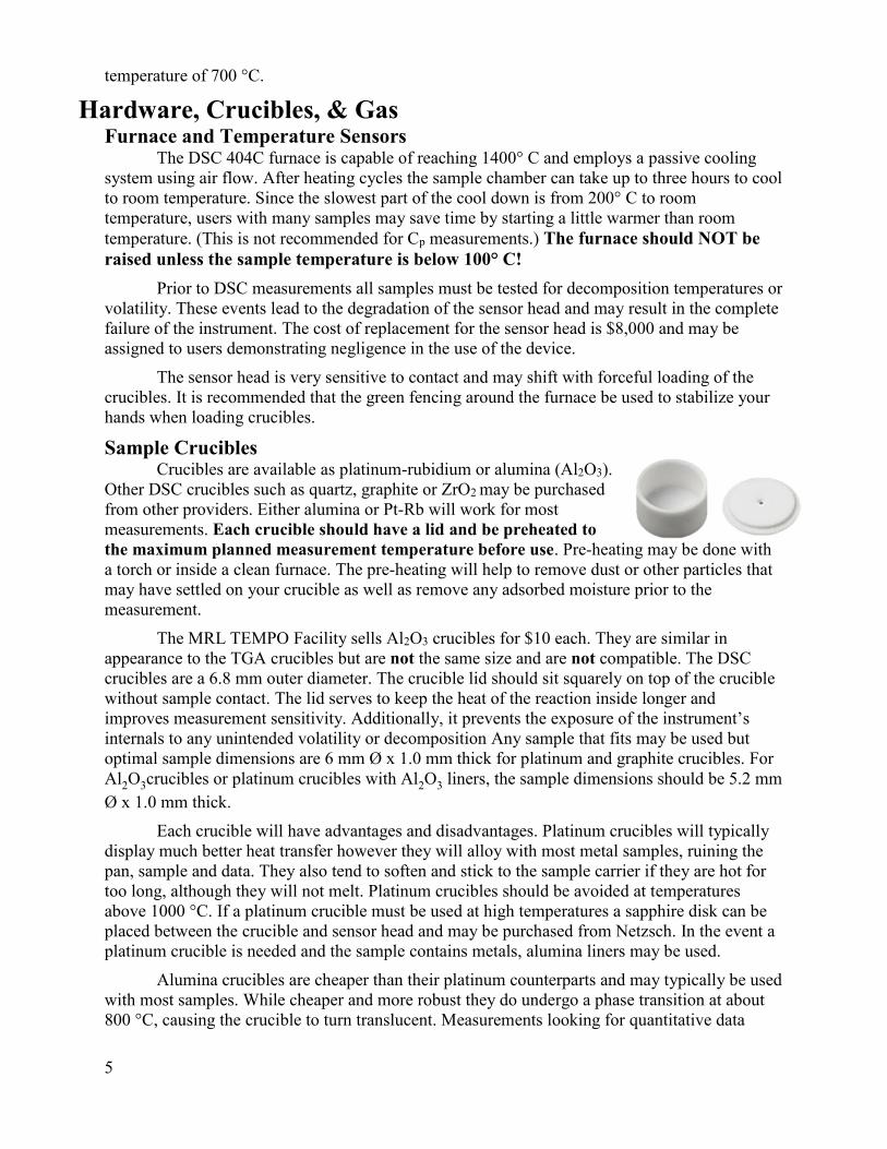
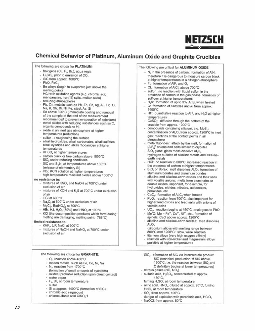
Sample Crucibles Crucibles are available as platinum-rubidium or alumina (Al2O3).
Other DSC crucibles such as quartz, graphite or ZrO2 may be purchased
from other providers. Either alumina or Pt-Rb will work for most
measurements. Each crucible should have a lid and be preheated to
the maximum planned measurement temperature before use. Pre-heating may be done with
a torch or inside a clean furnace. The pre-heating will help to remove dust or other particles that
may have settled on your crucible as well as remove any adsorbed moisture prior to the
measurement.
The MRL TEMPO Facility sells Al2O3 crucibles for $10 each. They are similar in
appearance to the TGA crucibles but are not the same size and are not compatible. The DSC
crucibles are a 6.8 mm outer diameter. The crucible lid should sit squarely on top of the crucible
without sample contact. The lid serves to keep the heat of the reaction inside longer and
improves measurement sensitivity. Additionally, it prevents the exposure of the instrument’s
internals to any unintended volatility or decomposition Any sample that fits may be used but
optimal sample dimensions are 6 mm Ø x 1.0 mm thick for platinum and graphite crucibles. For
Al2O3crucibles or platinum crucibles with Al2O3 liners, the sample dimensions should be 5.2 mm
Ø x 1.0 mm thick.
Each crucible will have advantages and disadvantages. Platinum crucibles will typically
display much better heat transfer however they will alloy with most metal samples, ruining the
pan, sample and data. They also tend to soften and stick to the sample carrier if they are hot for
too long, although they will not melt. Platinum crucibles should be avoided at temperatures
above 1000 °C. If a platinum crucible must be used at high temperatures a sapphire disk can be
placed between the crucible and sensor head and may be purchased from Netzsch. In the event a
platinum crucible is needed and the sample contains metals, alumina liners may be used.
Alumina crucibles are cheaper than their platinum counterparts and may typically be used
with most samples. While cheaper and more robust they do undergo a phase transition at about
800 °C, causing the crucible to turn translucent. Measurements looking for quantitative data
6
around that temperature should opt for another crucible choice. Specific heat capacity
measurements that require heating through that region may find increasing error as they move
above the transition temperature.
Extreme care must be taken to ensure that no crucible/sample reaction will
occur before running the sample in the DSC. One of the major causes of measuring head
(sensor) death is crucible/sample reaction. The sensor replacement cost is approximately $8,000.
If in doubt, heat the sample in a crucible in a lab furnace before trying it in the DSC. The Faculty
advisor of a negligent user who damages the DSC may be required to pay the cost of repair. A
guide on crucible selection can be found on the TEMPO Instrument Training and Resources page
on Gauchospace as well as in the appendix of this manual.
Standards for Heat Capacity There is a black and clear plastic box (about 2" x 1.5" x 0.75") in the DSC drawer which
should have four sapphire standards of varying thickness and two Al2O3 standards. Use the
sapphire standard with a thickness that measures closest to the sample. If in doubt, use the 0.50
mm sapphire standard.
Atmosphere for Tests The DSC can work in using several gases but argon is suitable for almost all tests. Some
users like to use air as a process gas to prevent sample reduction. The systems default setup uses
either Argon on Purge 1 or clean dry air on Purge 2. Other suitable gasses are nitrogen and
oxygen. Nitrogen is available in the lab but may form nitrosyl compounds at temperatures
beyond 700°C. Users interested in using oxygen would need to supply their own gas.
For tests requiring extremely high sensitivity helium serves as a completely inert gas with
excellent thermal conductivity. Users interested in helium would need to supply their own gas.
Please contact the MRL staff if you have questions about other gasses.
Sample Preparation Samples must be tested for decomposition or volatility in the TGA prior to use and the
data and results confirmed by a TEMPO staff member. Decomposition can lead to deposit
buildup within the device and degrade instrument sensitivity. Some compounds may react with
the sensor head damaging or destroying it. The use of a crucible lid helps to safeguards the
device. Users should consider four basic principles during sample preparation:
1. Selecting the right crucible.
2. Making and maintaining good thermal conduct between the sample and crucible.
3. Preventing contamination of the outer surfaces of the crucibles.
4. The influence of the atmosphere surrounding the sample.
Thermal Contact Ideally samples are flat disks, powders or pellets with disks typically demonstrating
better heat transfer. The sample should be flat to insure good thermal contact with the crucible
floor. Powders may undergo sintering during the heating process and then deform, losing thermal
contact with the crucible. Thin films may also display curling or curvature upon heating, causing
a loss of thermal contact. A sample of minimal thickness and maximum flat surface area is
desired.
Irregularly shaped samples may be optimized by sawing and grinding surfaces intended
to contact the crucible floor. More brittle substances may be ground to a fine powder and then
compacted into the crucible.
7
Method Development Basic Measurement Requirements Although the DSC is functionally quite simple, a good measurement requires some
variation in methodology. Some basic guidelines for measurement criteria are:
For the Transition Enthalpy (aka Latent Heat).
• Sample & Crucible mass
• Temperature Calibration file
• Sensitivity file
• A Baseline Correction measurement.
• Sample measured as Sample+Correction
For the Specific Heat (aka Heat Capacity or Cp):
• Sample & Crucible mass
• Temperature Calibration file
• Baseline Correction
• Heat Capacity Standard measured as Sample + Correction
• Sample measured as Sample + Correction
For the temperatures (Onset, Peak, Endset) of Melting & Phase Transformations and of Glass
Transition & Crystallization:
• Sample & Crucible mass
• Temperature Calibration file
• Sample measured as Sample
For the temperature and quantitative energy change of Melting & Phase Transformations and of
Glass Transition & Crystallization:
• Sample & Crucible mass
• Temperature Calibration file
• Sensitivity File.
• A Baseline Correction measurement.
• Sample measured as Sample+Correction

8
Phase Transition Measurements Measurements looking to determine the onset temperature of phase transitions are
typically robust and least likely to be affected by experimental errors. Users looking to obtain as
exact a value as possible should consider performing multiple runs in which they attempt to
narrow the temperature range over which they measure.
An example of this type of measurement might begin with an exploratory test in which
the material is heated over a range of ±50 °C of their expected transition temperature. Once a
crude temperature value has been reached then users may choose to rerun in a range of ± 30 °C.
By narrowing the range over which the measurement is made the user reduces the error produced
by thermal lag in the final value. Conversely if a phase transition were expected to occur at a
temperature of 900 °C and the user’s measurement range was from 100 – 1000 °C then the
accumulation of thermal lag in the material might lead to an erroneous melting point of 950 °C.
A general form for phase transition measurements is to first ramp to a value at least 20 °C
below the expected transition temperature and then hold at that temperature to equilibrate. Once
the contents of the furnace are equilibrated users may ramp the temperature over their anticipated
range.
Heat Capacity Measurements Similar to phase transition measurements, heat capacity measurements may also be
subject to thermal lag induced error. Users desiring to measure heat capacity over large ranges of
temperature may want to consider measuring heat capacity using a series of ramping periods
with intermittent isothermal intervals to allow for equilibrium in between. That is, if the
temperature range of interest is 500 – 1000 °C users may choose to heat the sample from 500 °C
to 600 °C and then hold the sample at 600 °C for ten minutes before heating the sample again, up
to 700 °C. This method helps to reduce the accumulation of thermal lag over long measurements.
Possible Issues Theoretically a first order phase transition, such as melting or recrystallization, can be
measured as many times as desired however this depends on two principles which may not
always hold true.
1. Upon cooling the sample returns to its original state.
2. The sample does not demonstrate any evaporation, sublimation, reaction or other
decomposition during the measurement.

9
Hardware
Instrument Components
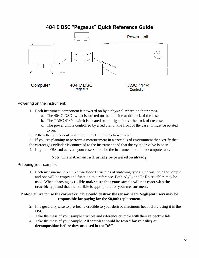
Using the Instrument Powering the Instrument On The instrument should be given about 15 minutes to warm up after powering on. Each
instrument component is powered on by physical switches located on their respective cases.
1. The power unit is controlled by a red dial on the front of the case. It must be
rotated to on.
2. The TASC 414/4 switch is located on the right side at the back of the case.
3. The 404 C DSC switch is located on the left side at the back of the case.
Operating the Furnace The DSC furnace is raised and lowered using the two arrow buttons located on the front
of the device in combination with the safety button on the ride side panel of the furnace base.
The safety button and arrow button must both be pressed to move the furnace. Users should
confirm that the vacuum indicator (to the right of the arrow buttons) does not have a red light on.
If the furnace is under vacuum it should not be opened.
Once the furnace has been raised, and the crucibles loaded the furnace may be lowered
again. Prior to fully lowering the furnace users should visually confirm that it will not
contact the measuring head. Once the furnace has been fully lowered a green light should
appear in the arrow button of the furnace base. If the light does not turn on check to make sure
that the furnace is fully lowered. Users should not raise the furnace unless it is below 100
°C.
10
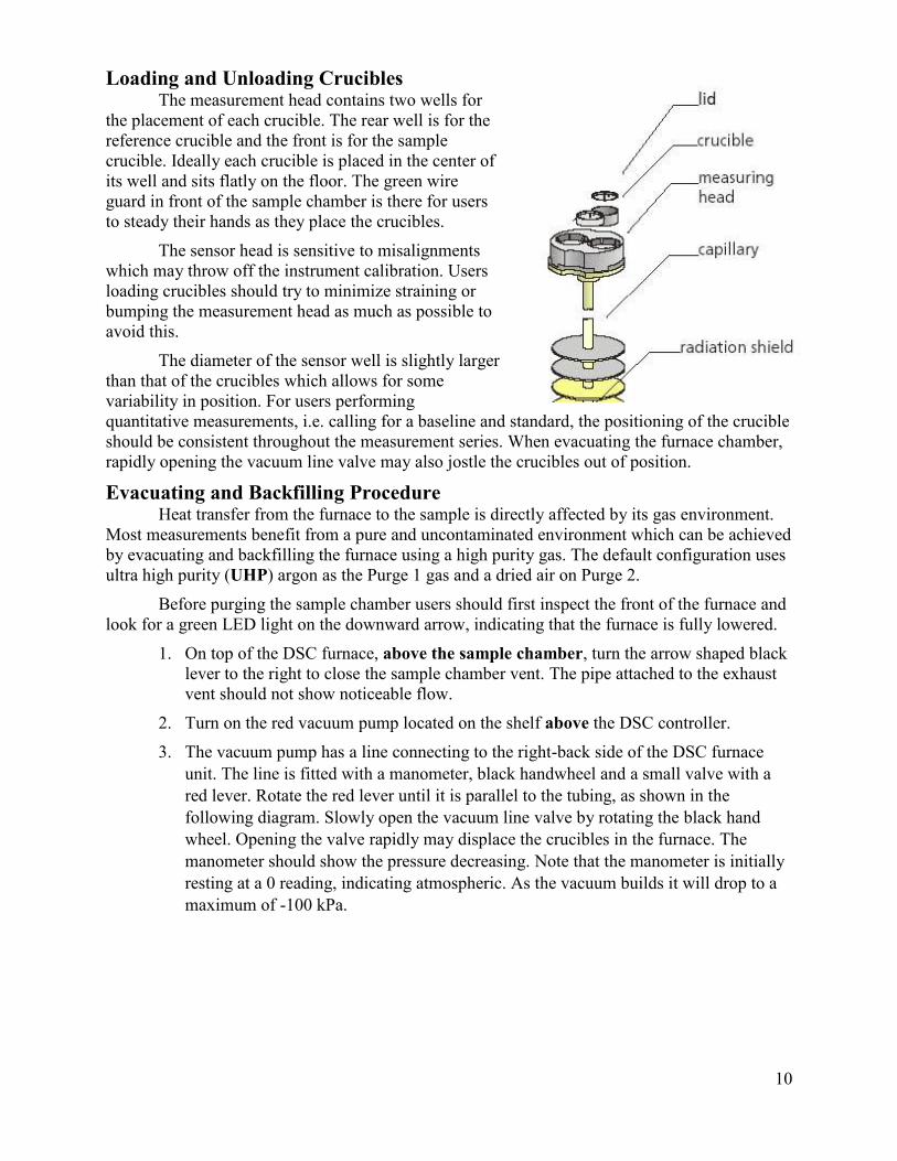
Loading and Unloading Crucibles The measurement head contains two wells for
the placement of each crucible. The rear well is for the
reference crucible and the front is for the sample
crucible. Ideally each crucible is placed in the center of
its well and sits flatly on the floor. The green wire
guard in front of the sample chamber is there for users
to steady their hands as they place the crucibles.
The sensor head is sensitive to misalignments
which may throw off the instrument calibration. Users
loading crucibles should try to minimize straining or
bumping the measurement head as much as possible to
avoid this.
The diameter of the sensor well is slightly larger
than that of the crucibles which allows for some
variability in position. For users performing
quantitative measurements, i.e. calling for a baseline and standard, the positioning of the crucible
should be consistent throughout the measurement series. When evacuating the furnace chamber,
rapidly opening the vacuum line valve may also jostle the crucibles out of position.
Evacuating and Backfilling Procedure Heat transfer from the furnace to the sample is directly affected by its gas environment.
Most measurements benefit from a pure and uncontaminated environment which can be achieved
by evacuating and backfilling the furnace using a high purity gas. The default configuration uses
ultra high purity (UHP) argon as the Purge 1 gas and a dried air on Purge 2.
Before purging the sample chamber users should first inspect the front of the furnace and
look for a green LED light on the downward arrow, indicating that the furnace is fully lowered.
1. On top of the DSC furnace, above the sample chamber, turn the arrow shaped black
lever to the right to close the sample chamber vent. The pipe attached to the exhaust
vent should not show noticeable flow.
2. Turn on the red vacuum pump located on the shelf above the DSC controller.
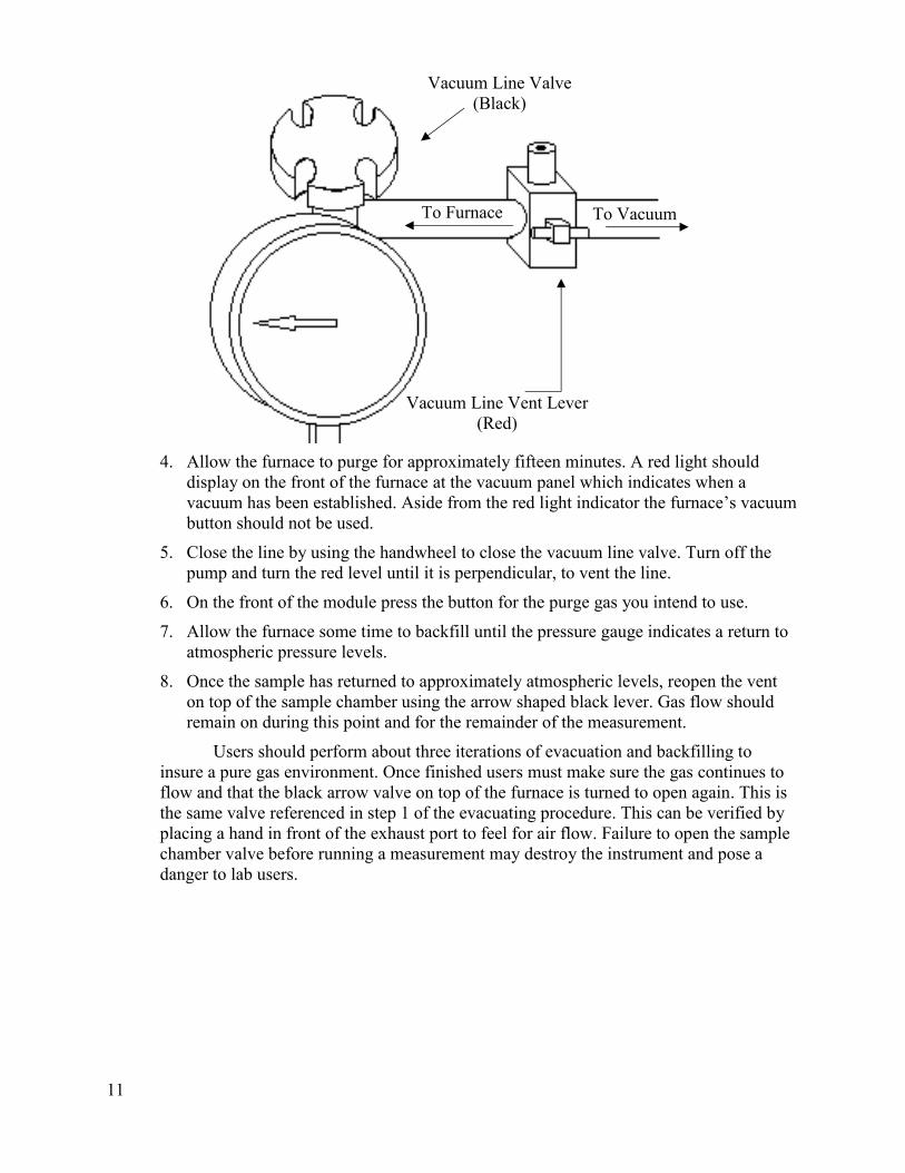
3. The vacuum pump has a line connecting to the right-back side of the DSC furnace
unit. The line is fitted with a manometer, black handwheel and a small valve with a
red lever. Rotate the red lever until it is parallel to the tubing, as shown in the
following diagram. Slowly open the vacuum line valve by rotating the black hand
wheel. Opening the valve rapidly may displace the crucibles in the furnace. The
manometer should show the pressure decreasing. Note that the manometer is initially
resting at a 0 reading, indicating atmospheric. As the vacuum builds it will drop to a
maximum of -100 kPa.
11
4. Allow the furnace to purge for approximately fifteen minutes. A red light should
display on the front of the furnace at the vacuum panel which indicates when a
vacuum has been established. Aside from the red light indicator the furnace’s vacuum
button should not be used.
5. Close the line by using the handwheel to close the vacuum line valve. Turn off the
pump and turn the red level until it is perpendicular, to vent the line.
6. On the front of the module press the button for the purge gas you intend to use.
7. Allow the furnace some time to backfill until the pressure gauge indicates a return to
atmospheric pressure levels.
8. Once the sample has returned to approximately atmospheric levels, reopen the vent
on top of the sample chamber using the arrow shaped black lever. Gas flow should
remain on during this point and for the remainder of the measurement.
Users should perform about three iterations of evacuation and backfilling to
insure a pure gas environment. Once finished users must make sure the gas continues to
flow and that the black arrow valve on top of the furnace is turned to open again. This is
the same valve referenced in step 1 of the evacuating procedure. This can be verified by
placing a hand in front of the exhaust port to feel for air flow. Failure to open the sample
chamber valve before running a measurement may destroy the instrument and pose a
danger to lab users.
To Furnace To Vacuum
Vacuum Line Vent Lever
(Red)
Vacuum Line Valve
(Black)
12
Software The DSC uses two applications, one for measurements and the other for analysis. The
icons of both programs, DSC 404C and Proteus Analysis, are located on the desktop of the
computer. Data may be accessed by transferring it to the TEMPO network hard drive, also
located on the desktop.
The DSC 404C program is used to communicate with the DSC and perform the
measurements. Sample data and thermal programming are entered through this software which
then collects the data. All data is saved in a temporary file until the completion of the
measurement making the computer sensitive to memory use during collection. Users should
avoid use of the computer during measurement to prevent data loss.
To start a new measurement, open the DSC 404C software and from the top menu select
new measurement. This will open the DSC 404C Measurement Header to begin designing a
measurement program.
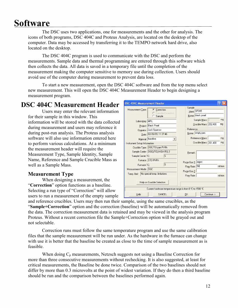
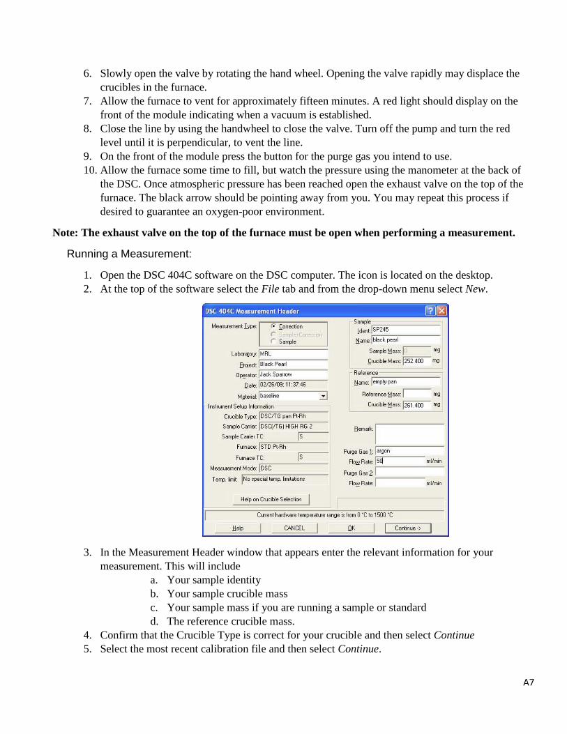
DSC 404C Measurement Header Users may enter the relevant information
for their sample in this window. This
information will be stored with the data collected
during measurement and users may reference it
during post-run analysis. The Proteus analysis
software will also use information entered here
to perform various calculations. At a minimum
the measurement header will require the
Measurement Type, Sample Identity, Sample
Name, Reference and Sample Crucible Mass as
well as a Sample Mass.
Measurement Type When designing a measurement, the
“Correction” option functions as a baseline.
Selecting a run type of “Correction” will allow
users to run a measurement of the empty sample
and reference crucibles. Users may then run their sample, using the same crucibles, as the
“Sample+Correction” option and the correction (baseline) will be automatically removed from
the data. The correction measurement data is retained and may be viewed in the analysis program
Proteus. Without a recent correction file the Sample+Correction option will be grayed out and
not selectable.
Correction runs must follow the same temperature program and use the same calibration
files that the sample measurement will be run under. As the hardware in the furnace can change
with use it is better that the baseline be created as close to the time of sample measurement as is
feasible.
When doing Cp measurements, Netzsch suggests not using a Baseline Correction for
more than three consecutive measurements without rechecking. It is also suggested, at least for
critical measurements, the Baseline be done twice. Comparison of the two baselines should not
differ by more than 0.3 microvolts at the point of widest variation. If they do then a third baseline
should be run and the comparison between the baselines performed again.

13
Measurements looking for onset temperatures of thermal events generally do not require
corrections and may run using the measurement type “Sample”.
Sample Information Many of the fields, such as laboratory and project are for user reference and do not need
to filled in. The material field is included in this and whatever entry is used does not affect future
measurements or calculations. The gas flow rate field also does not affect any system settings
but does allow users to note what parameters they chose to run at for future reference. The
default setting for gas flow rate is approximately 75 mL/min.
Users should confirm that their crucible type is correct for their intended measurement
and that the sample carrier field has “DSC(/TG) HIGH RG 2” written in. If something else is
displayed then please inform the MRL staff before using the instrument.
Once the appropriate fields have been filled users may press Continue to move to the next
step and select a temperature calibration. Selecting OK will abruptly end they measurement
configuration.
Temperature Calibration & Sensitivity Files When designing a measurement, users will be required to specify a Temperature and
Sensitivity Calibration file. The Temperature Calibration selection window will
automatically open to the correct folder and the most recent temperature calibration file should
be chosen.
Temperature Calibration File Multiple calibration files may be present, each attenuated to specific temperature ranges
and testing conditions. The user should select the temperature calibration file that covers their
desired temperature range and was performed in similar conditions including:
• Crucible type
• Gas environment
• Heating rate
If unable to find an appropriate temperature calibration for the intended measurement,
please speak with the MRL staff about having one made. Currently the DSC has calibration files
designed for use with Al2O3 crucibles which are appropriate for most phase transition
measurements. Samples that are incompatible with alumina may be run in the Pt-Rb crucibles
however these pans often alloy with the metal standards used to make the calibration files. Users
will need to purchase alternative standards for use with the Pt-Rb pans.
Sensitivity File A sensitivity calibration file is required if the user wants quantitative energy information
from their measurement. For phase transition measurements, which only look at temperature-
event relationships, the Senzero file may be selected. Quantitative measurements require a
sensitivity file that matches the measurements parameters as closely as possible. When a
sensitivity file is selected users may measure energy changes in mW/mg and integrate peak areas
in joules/gram.
The creation of a sensitivity calibration file is an involved process that requires
measurements of five to six standards. If you plan on doing quantitative measurements please
verify that an appropriate sensitivity file is already present. Users who need a new sensitivity file
should speak with the MRL staff at least a week in advance of their intended measurement.

14
Temperature Programming
Temperature programs are composed of, at minimum:
• The Initial Standby/Initial
• An Isothermal Step
• A Dynamic Step
• The Final Emergency Setting
• The Final Standby
The initial step sets the temperature value that data begins recording at. Once the
measurement program is started the initial temperature step begins but data will only be recorded
once it has reached the “initial” value. That is, if you initially heat to 400 °C and specify an
initial value of 360 °C then data will not be recorded until 360 °C is reached. It is recommended
that users go no lower than 40 °C for their initial temperatures due to low heat limitations of the
furnace heating element.
Initial Standby is an alternative to the initial step. This step allows users to instruct the
furnace to heat to a given temperature and then hold that for a set of time prior to recording data.
This performs similar to an unrecorded isothermal step but may be used to pre-heat the sample
chamber prior to introducing the sample. Either initial or initial standby may be used. Most
measurements will use the initial step.
The isothermal step programs the DSC to hold the sample chamber at its current
temperature for a designated period of time. These are often used to allow the sample chamber to
stabilize following or preceding a dynamic step. Preceding and following a dynamic step with
isothermals of 10 to 15 minutes can decrease percent error in measurements.
Dynamic steps are where ramp rates or heating rates are designated. A target temperature
is selected, as well as a heating rate. Notice that the target temperature is in °C and the heating
rate is in K/min. Ramping speed can be changed based on interest in a specific temperature
range. For ranges containing data of interest a ramping rate of 10-20 K/minute is recommend. A
faster rate may be set, such as 30 K/minute, for regions without interest. The instrument is
capable of 40 K/minute however this stresses the heating element and may cause the sample
15
chamber to overshoot the desired temperature. During dynamic steps with a decreasing
temperature (ie from 700 °C to 600 °C) the DSC employs passive cooling. Setting a heating rate
of 10 K/min will instruct the DSC to attempt to keep the cooling to approximately that value. It
is recommended that each dynamic step be preceded by an isothermal to allow the temperature
of the sample and sample chamber to equilibrate.
Isothermal and dynamic steps also require a pts/min parameter which tells the instrument
how often to record a data point during the step. Data acquisition rates can be changed based on
interest in a specific temperature range. It may be entered as either points per degree or per
minute. 60 points per minute is generally appropriate for sections of interest. The system has a
limit of 24000 data points per measurement that it will notify you of, should your program go
beyond that.
The Final step sets a safeguard temperature for the measurement. This will auto-populate
with a value 10 °C higher than your highest temperature. If the instrument reaches this
temperature it will automatically terminate the sequence as an effort to prevent damage to the
instrument and sample. Final Standby programs the DSC with instructions on what to do once
the sample has finished. The instrument will drop to the stand-by temperature at the heating rate
designated, and attempt to hold it there for the given time. As this should always be a cooling
step, the heating rate can be set to 40.0 K/min to allow the system to cool quickly and shorten the
time needed per measurement.
Possible Issues There are often anomalies in the data at points where the furnace heating range changes
so users should set temperature programs with steady heating rates that go at least 20 °C beyond
your desired end point. Shorter dynamic steps allow for an increase in measurement accuracy but
run the risk of cutting off phase transition events prematurely or missing them altogether.
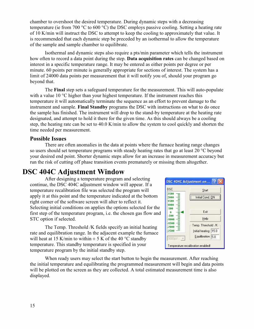
DSC 404C Adjustment Window After designing a temperature program and selecting
continue, the DSC 404C adjustment window will appear. If a
temperature recalibration file was selected the program will
apply it at this point and the temperature indicated at the bottom
right corner of the software screen will alter to reflect it.
Selecting initial conditions on applies the options selected for the
first step of the temperature program, i.e. the chosen gas flow and
STC option if selected.
The Temp. Threshold /K fields specify an initial heating
rate and equilibration range. In the adjacent example the furnace
will heat at 15 K/min to within ± 5 K of the 40 °C standby
temperature. This standby temperature is specified in your
temperature program by the initial standby step.
When ready users may select the start button to begin the measurement. After reaching
the initial temperature and equilibrating the programmed measurement will begin and data points
will be plotted on the screen as they are collected. A total estimated measurement time is also
displayed.

16
Measurement Conclusion Once your measurement has finished the program will automatically save the data in the
user designated location. Users should wait until the furnace has cooled to a safe temperature of
40 °C before attempting to remove their sample.
Users should not turn off any component of the DSC once completing a measurement.
Shutting off the furnace power transformer before the furnace reaches a value below 500 °C will
permanently damage the device.
The Proteus Analysis Program Data analysis can be performed on the Netzsch Proteus Software, located on the desktop.
Once a run has completed the data is automatically saved. The save location is chosen prior to
starting the measurement.
To analyze their data users should open the Proteus software by double clicking the icon
at the center of the desktop. Once open users may open their data by selecting either File, from
the menu at the top of the screen, or the folder icon in the toolbar.
The Proteus Interface
An example of a DSC measurement is shown below. The shown sample is heated to a
peak of 500°C after a 10-minute equilibration period. The dotted red line shows the temperature
over time and the blue shows the signal difference between the reference and tested material in
units of µV/mg. Notice the phase transition around 440°C.
Curves may be right clicked to bring up some menu options for manipulation. Selecting
the curve properties option will allow the user to customize the color and appearance of the line
while the file properties option will bring up a window containing all of the measurement data
stored in the file. This includes the user created temperature program and all the parameters that
the measurement was performed under.

17
The software automatically displays time along the x-axis when opening new data
however users looking for onset temperatures of transitions can display temperature as the x-axis
by selecting the button in the toolbar. This will cut your measurement into segments with
each segment corresponding to one step in the temperature program. Isothermal segments will
automatically be hidden as these will consist of a flat line.
Users wishing to high (or unhide) a line segment may right click on the curve and select
view segments. This will produce a window listing each segment which users may check or
uncheck to display.
Exporting Data
Experimental results may be exported as either an ASCII or ANSI Unicode file.
Typically, users will want to select ASCII and then choose the .csv format. This will export their
data as a comma separated values file which may then be opened in excel.
To export the data, select the Extras option from the toolbar at the top of the Proteus
window. In the drop down menu choose Export Data. Fill out the dialog box that should pop up
and choose where you would like to export your data to.
Retrieving Data To maintain the integrity of our instrument computers, USB access is disabled. Instead
each instrument has access to a shared TEMPO hard drive, with a shortcut present on the
desktop. Users may access that hard drive, from the instrument, and make a folder for
themselves. They can then copy all data from the instrument computer to the shared hard drive.
This hard drive may then be access by the shared computer in TEMPO labs, and data can be
retrieved there using a USB device.

18
Analyzing DSC Data Anatomy of a Peak
A DSC event peak typically contains the following components:
• Baseline: This is the expected signal (or change in signal) if no transition event occurs (e.g. if
the enthalpy change of melting or Hfusion were zero). This is not always a flat line, as the
specific heat capacity of a material is not guaranteed to be constant as temperature changes,
or after a phase transition.
• First Tangent Line: This line is generated by an analytical program, (Proteus) and attempts
to project a tangent along the most reasonable length of the phase transition’s first peak. The
criteria for “reasonable” in this scenario would be the longest length of approximately
consistent slope.
• Second Tangent Line: Similar to the first tangent line, this is a projection along the second
length of the peak using similar methods. This is also generated by an analytical program.
• Onset: The onset of a transition event is where the tangent line intersects the baseline. Users
may want to use the first tangent line to look at the onset of a melting transition or use the
second tangent line to look at the onset of a recrystallization event.
• Endset: The endset of an event occurs at the intersection of the tangent line with the baseline
on the second half of a peak. Like the onset, users may choose the second tangent line to find
the endset of a melting transition or the first tangent line to find the end point of a
recrystallization event.
• Peak Apex: The location of the max peak value is subject to multiple variables. Its value is
influenced by the thermal kinetics of the sample and the DSC system. The sample mass,
shape, density, and crucible contact as well as the heating rate and gas environment will all
impact at what temperature or time the phase transition will reach itss maximum. As a result
it is generally a poor indicator of a sample’s properties.
Using Proteus Identifying Transition Events Once a file is initially opened in Proteus the default display uses intervals of time on the
x-axis and both temperature and signal along either y-axis. For the purposes of analyzing
transition events users will find it much more useful to view the data using temperature as the x-
Extrapolated Peak
Second Tangent Line First Tangent Line
Onset Endset
Baseline

19
axis. Before the axis can be altered users will need to split the segments, hide isothermal portions
and, if needed, spline segments together.
Splitting a Curve into Segments To cut a measurement curve into segments, using Proteus, users will need to left-click on
their curve of interest, causing it to turn white. Then, users will right click on the same curve to
display a menu. From this menu select the “Split Into Segments” option. The curve should now
be cut into multiple segments, of different colors, corresponding to each step in the programmed
measurement. That is each segment corresponds to a dynamic or isothermal step according to the
program used to gather the data.
Selecting & Hiding Segments Once a curve is broken into its
various steps each segment or set of
segments may be selected or hidden.
Right clicking on the background of the graph (the gray area) will open another menu allowing
users to open the Segments window. This window will show a list of the various segments that
the curve has been cut into. Selecting or deselecting the check boxes next to each segment will
allow users to hide or portion.
Generally if users are interested in looking at transition events they can uncheck the
initial heating periods and any isothermal segments that do not contain portions of the relevant
peaks. For transition events with peaks that spill over into two segments, the segment will
needed to be splined.
20
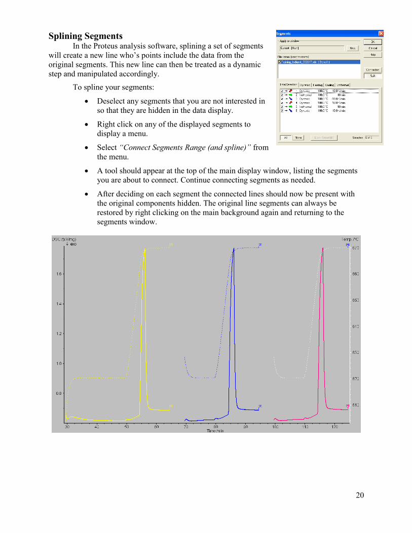
Splining Segments In the Proteus analysis software, splining a set of segments
will create a new line who’s points include the data from the
original segments. This new line can then be treated as a dynamic
step and manipulated accordingly.
To spline your segments:
• Deselect any segments that you are not interested in
so that they are hidden in the data display.
• Right click on any of the displayed segments to
display a menu.
• Select “Connect Segments Range (and spline)” from
the menu.
• A tool should appear at the top of the main display window, listing the segments
you are about to connect. Continue connecting segments as needed.
• After deciding on each segment the connected lines should now be present with
the original components hidden. The original line segments can always be
restored by right clicking on the main background again and returning to the
segments window.
21
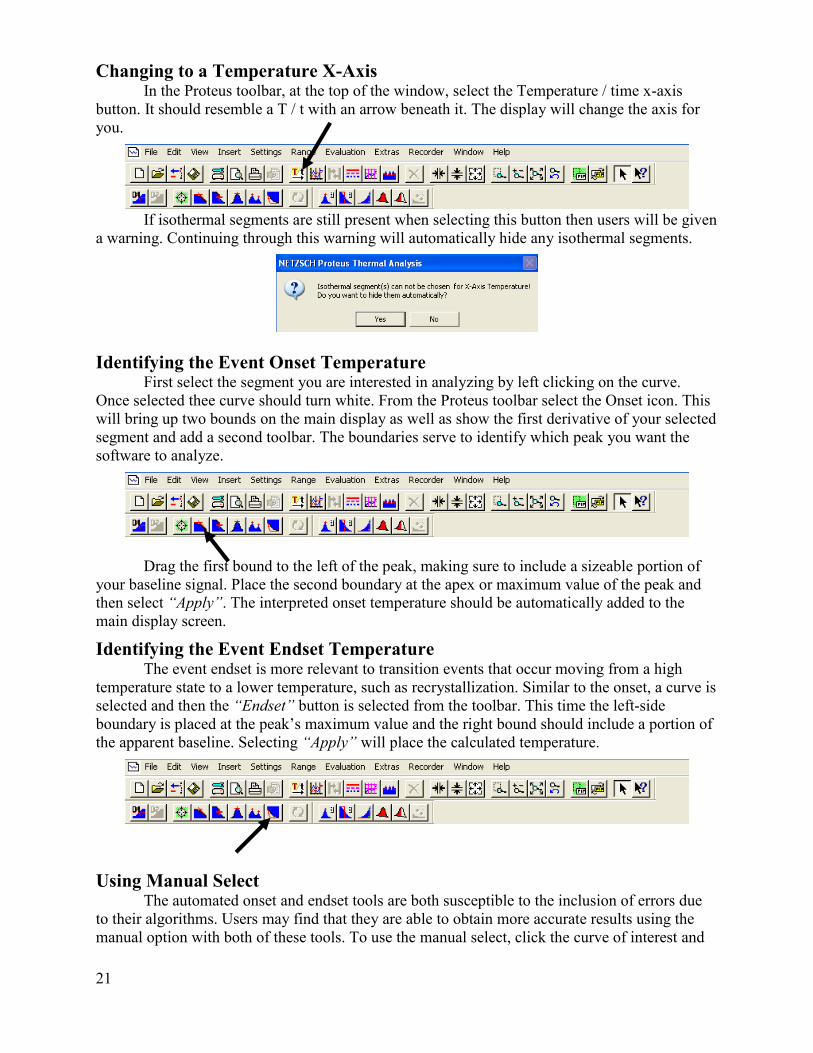
Changing to a Temperature X-Axis In the Proteus toolbar, at the top of the window, select the Temperature / time x-axis
button. It should resemble a T / t with an arrow beneath it. The display will change the axis for
you.
If isothermal segments are still present when selecting this button then users will be given
a warning. Continuing through this warning will automatically hide any isothermal segments.
Identifying the Event Onset Temperature First select the segment you are interested in analyzing by left clicking on the curve.
Once selected thee curve should turn white. From the Proteus toolbar select the Onset icon. This
will bring up two bounds on the main display as well as show the first derivative of your selected
segment and add a second toolbar. The boundaries serve to identify which peak you want the
software to analyze.
Drag the first bound to the left of the peak, making sure to include a sizeable portion of
your baseline signal. Place the second boundary at the apex or maximum value of the peak and
then select “Apply”. The interpreted onset temperature should be automatically added to the
main display screen.
Identifying the Event Endset Temperature The event endset is more relevant to transition events that occur moving from a high
temperature state to a lower temperature, such as recrystallization. Similar to the onset, a curve is
selected and then the “Endset” button is selected from the toolbar. This time the left-side
boundary is placed at the peak’s maximum value and the right bound should include a portion of
the apparent baseline. Selecting “Apply” will place the calculated temperature.
Using Manual Select The automated onset and endset tools are both susceptible to the inclusion of errors due
to their algorithms. Users may find that they are able to obtain more accurate results using the
manual option with both of these tools. To use the manual select, click the curve of interest and

22
select the onset or endset tool of interest. In the toolbar that drops down check the box next to
“Manual”.
There should now be two set of bounds present on the display; a blue pair and a black
pair. The blue bounds identify the portion of the curve that the software will use as the peak
baseline. Ideally the user should highlight a region with a mostly consistent slope that is not too
far from the peak. The black bounds are used to highlight the portion of the peak that would
produce a tangent line most resembling the slope of the peak. Selecting apply will draw the new
tangent line and give the event’s temperature value.
23
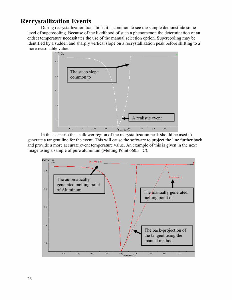
Recrystallization Events During recrystallization transitions it is common to see the sample demonstrate some
level of supercooling. Because of the likelihood of such a phenomenon the determination of an
endset temperature necessitates the use of the manual selection option. Supercooling may be
identified by a sudden and sharply vertical slope on a recrystallization peak before shifting to a
more reasonable value.
In this scenario the shallower region of the recrystallization peak should be used to
generate a tangent line for the event. This will cause the software to project the line further back
and provide a more accurate event temperature value. An example of this is given in the next
image using a sample of pure aluminum (Melting Point 660.3 °C).
The steep slope
common to
supercooling.
A realistic event
slope.
The automatically
generated melting point
of Aluminum The manually generated
melting point of
Aluminum
The back-projection of
the tangent using the
manual method
24
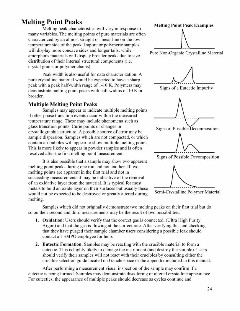
Melting Point Peaks Melting peak characteristics will vary in response to
many variables. The melting points of pure materials are often
characterized by an almost straight or linear line on the low
temperature side of the peak. Impure or polymeric samples
will display more concave sides and longer tails, while
amorphous materials will display broader peaks due to size
distribution of their internal structural components (i.e.
crystal grains or polymer chains).
Peak width is also useful for data characterization. A
pure crystalline material would be expected to have a sharp
peak with a peak half-width range of 1-10 K. Polymers may
demonstrate melting point peaks with half-widths of 10 K or
broader.
Multiple Melting Point Peaks Samples may appear to indicate multiple melting points
if other phase transition events occur within the measured
temperature range. These may include phenomena such as
glass transition points, Curie points or changes in
crystallographic structure. A possible source of error may be
sample dispersion. Samples which are not compacted, or which
contain air bubbles will appear to show multiple melting points.
This is more likely to appear in powder samples and is often
resolved after the first melting point measurement.
It is also possible that a sample may show two apparent
melting point peaks during one run and not another. If two
melting points are apparent in the first trial and not in
succeeding measurements it may be indicative of the removal
of an oxidative layer from the material. It is typical for most
metals to hold an oxide layer on their surfaces but usually these
would not be expected to be destroyed or greatly altered during
melting.
Samples which did not originally demonstrate two melting peaks on their first trial but do
so on their second and third measurements may be the result of two possibilities.
1. Oxidation: Users should verify that the correct gas is connected, (Ultra High Purity
Argon) and that the gas is flowing at the correct rate. After verifying this and checking
that they have purged their sample chamber users considering a possible leak should
contact a TEMPO employee for help. 2. Eutectic Formation: Samples may be reacting with the crucible material to form a
eutectic. This is highly likely to damage the instrument (and destroy the sample). Users
should verify their samples will not react with their crucibles by consulting either the
crucible selection guide located on Gauchospace or the appendix included in this manual. After performing a measurement visual inspection of the sample may confirm if a
eutectic is being formed. Samples may demonstrate discoloring or altered crystalline appearance.
For eutectics, the appearance of multiple peaks should decrease as cycles continue and
Melting Point Peak Examples
Pure Non-Organic Crystalline Material
Signs of a Eutectic Impurity
Signs of Possible Decomposition
Signs of Possible Decomposition
Semi-Crystalline Polymer Material

25
homogeneity is established however the final peak will be representative of the newly formed
sample’s properties and not the original materials.
Polymorphism Solid samples capable of existing in more than one form or crystal structure may produce
two noticeable peaks (and onset points) during phase transitions. In this scenario the baseline
used to interpret the first peak is also used on the second.
Overlapping Peaks If two events or peaks overlap a better resolution may be achieved by alternating heating
rates during the measurement. Either higher or lower heating rates may be used. The
measurement could also be rerun with a smaller quantity of sample.
Recrystallization Point Peaks Integration of recrystallization peaks should
produce an area similar in size to the corresponding
melting point peaks. Some differences may appear as a
result of supercooling but the peak area should not
deviate by more than 20%.
It is common for samples to show some level of
supercooling effects during recrystallization. This is
typically manifested by a difference between measured
melting point and recrystallization. A reasonable
range of disagreement would be 1-50 K. Substances
that crystallize rapidly after nucleation would be
expected to have a sharp and vertical peak before
establishing a more gradual slope. Because of this
supercooling effect users looking to establish a
recrystallization point will need to project backwards
from this shallower region.
Materials that demonstrate amorphous
solidification (i.e. form glasses on cooling) will not
demonstrate easily noticeable peaks but instead will show
a sudden change in specific heat capacity or shift in the
baseline. Samples with eutectic impurities which solidify
this way don’t show their characteristic two peaks.
Multiple Recrystallization Point Peaks Samples that don’t completely cover the crucible
floor or which use small quantities of noble metals can
form individual drops in their liquid phase. Each of these
drops can exhibit different levels of supercooling and
form a series of smaller recrystallization peaks. The total
area under these peaks should still approximately match
the of the melting point. Measurements may benefit from
rerunning the sample using more material or ensuring
even distribution across the crucible floor.
Recrystallization Point Peak Examples
a Pure Non-Organic Crystalline Material
a Material with a Eutectic Impurity
a Semi-Crystalline Polymer Material
a Material Showing Multiple Supercooling Effects

26
Other Possible Peak Events Glass Transition Points (Tg) The glass transition point is the temperature at which an amorphous material undergoes
a transition from a brittle or hard state to a rubber-like viscous state. The transition is reversible
and is known as vitrification. Measurements for glass transition points will typically follow two
possible patterns.
1. Glass Transition: Peaks will show an abrupt and linear rise in
signal before quickly leveling out.
2. Glass Transition with Enthalpy Relaxation: After the initial
climb, the signal will drop again before leveling out. This is
more commonly seen in samples that have been stored for a
long period of time below the glass transition temperature.
Samples undergoing repeated cycles should only show this
event in the initial heating.
Transition events will typically occur over ranges of 10-30 K. Users suspecting that an
event might be a glass transition point can verify this by using a furnace or other heating source
to heat their samples to the event temperature and observing if the material has assumed a
noticeable elastic, softened or liquid like quality. Users should not use the DSC to do this, as the
furnace cannot be raised during a measurement or when the temperature exceeds 100 °C.
Reporting the temperature of the glass transition is, to some degree, based on preference.
No standard is currently established about which point along the curve is considered the official
“temperature”. Papers typically report either the onset, midpoint or endpoint temperature of the
transition.
It is also important to note that the glass transition temperature will vary by
instrumentation and technique. Measurement by means of a physical instrument, such as
dynamic mechanical analysis (DMA) will often report a higher temperature than a DSC. This is
due to the sensitivity of the detection method (mechanical versus electrical) and both
measurements can be considered accurate and precise. Users reporting a glass transition
temperature should also include the instrumentation and means of determining the temperature.
Curie Transition Points (TC) Lambda transitions, or second order solid-solid transitions, can
be difficult to detect on a DSC. Users looking to establish the
temperature of a ferromagnetic Curie transition might find the TGA
is capable of providing more exact data however the DSC may be of use for
measurements looking to quickly find a temperature range at lower cost.
The Curie transition temperature (TC) is the temperature at which a permanent magnetic
material loses its magnetic properties. The ordered magnetic moments found in ferromagnetic
materials become disordered above the Curie temperature effectively terminating the net dipole.
TC peaks are usually slight and easily missed in data. Users should be careful to give a large
buffer range when designing measurements to obtain the Curie temperature as artifacts may hide
or alter the data.
a Glass Transition Event
a Glass Transition Event with
Enthalpy Relaxation
a Curie Transition Event

27
Ending Notes Further Reading
For more information the TEMPO Gauchospace page on differential scanning
calorimetry contains several useful documents, a quick reference guide and a guide to selecting
the appropriate crucible type for your measurement. Users interested in using different operating
parameters or using a different method are encouraged to speak with TEMPO staff.
Mettler-Toledo’s website also contains a wealth of freely accessible documents and
papers on thermal analysis principles and methods.
Author Information This manual was written by Burton Sickler, for the Materials Research Laboratory’s
TEMPO facilities; a MRSEC funded facility at the University of California, Santa Barbara. For
questions, comments or to notify the author of errors please e-mail [email protected].

A0
Appendix
Accessing GauchoSpace .................................................................................... A1
DSC Applications .............................................................................................. A4
404 C DSC “Pegasus” Quick Reference Guide .................................................... A5
Temperature and Sensitivity Calibration Protocol ............................................. A9
Evaluation of the Measurements ................................................................................................................................ A16
Temperature Calibration ........................................................................................................................................ A17
Sensitivity Calibration ............................................................................................................................................ A18
Creation of a Temperature/Sensitivity Calibration File .............................................................................................. A20
Temperature Calibration ........................................................................................................................................ A20
Sensitivity Calibration ............................................................................................................................................ A24
A1
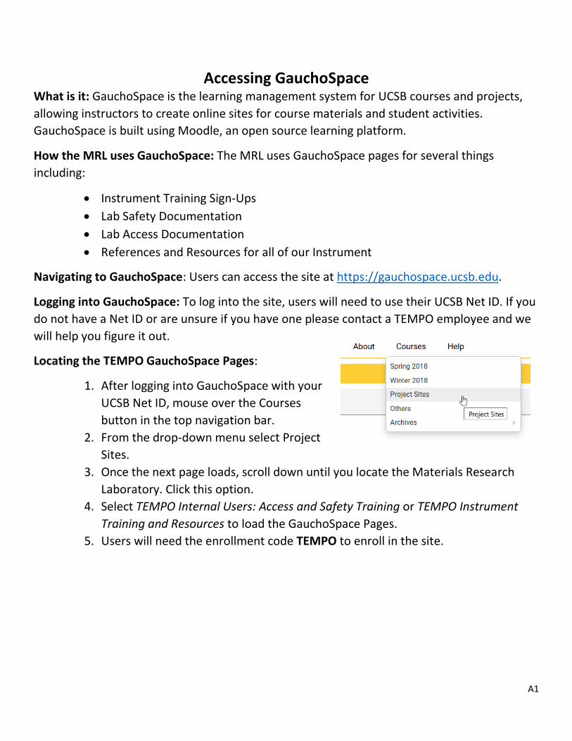
Accessing GauchoSpace What is it: GauchoSpace is the learning management system for UCSB courses and projects,
allowing instructors to create online sites for course materials and student activities.
GauchoSpace is built using Moodle, an open source learning platform.
How the MRL uses GauchoSpace: The MRL uses GauchoSpace pages for several things
including:
• Instrument Training Sign-Ups
• Lab Safety Documentation
• Lab Access Documentation
• References and Resources for all of our Instrument
Navigating to GauchoSpace: Users can access the site at https://gauchospace.ucsb.edu.
Logging into GauchoSpace: To log into the site, users will need to use their UCSB Net ID. If you
do not have a Net ID or are unsure if you have one please contact a TEMPO employee and we
will help you figure it out.
Locating the TEMPO GauchoSpace Pages:
1. After logging into GauchoSpace with your
UCSB Net ID, mouse over the Courses
button in the top navigation bar.
2. From the drop-down menu select Project
Sites.
3. Once the next page loads, scroll down until you locate the Materials Research
Laboratory. Click this option.
4. Select TEMPO Internal Users: Access and Safety Training or TEMPO Instrument
Training and Resources to load the GauchoSpace Pages.
5. Users will need the enrollment code TEMPO to enroll in the site.
A2

A3

A4
DSC Applications Property Method
Specific Heat Capacity as a function of time, Cp(t) Specific heat capacity (Cp)
Enthalpy-temperature function Enthalpy (ΔH)
Enthalpy changes, enthalpy of conversion Integration
Enthalpy of fusion, crystallinity, (ΔHfus) Integration, crystallinity
Melting Behavior (liquid content, liquid fraction) Integration (partial areas), Conversion
Melting point, solidus and liquidus point, (TM) Onset, Purity and Integration
Melting point of semi-crystalline plastics, (TM) Peak, Integration
Purity of non-crystalline plastics Purity
Melting point of the pure substance, (TM) Purity
Crystallization behavior, degree of crystallinity and supercooling Onset, Integration and Conversion
Solid-Solid transition, polymorphism Integration, Onset and Conversion
Vaporization, Sublimation and Desorption Integration and Conversion
Boiling Point, (TB) Peak, Onset and Integration
Glass transition, amorphous softening, (TG) Glass Transition (TG)
Curie temperature, temperature of a lambda transition, (TC) Peak and Integration
Thermal decomposition, pyrolysis, depolymerization Integration, Onset and Kinetics
Temperature Stability Onset, Integration and Kinetics
Chemical Reactions Integration and Kinetics
Reaction Enthalpy, (ΔHrxn) Integration
Oxidative degradation, oxidation stability, oxidation induction time Onset
Content Determination Content
A5
404 C DSC “Pegasus” Quick Reference Guide
Powering on the instrument:
1. Each instrument component is powered on by a physical switch on their cases.
a. The 404 C DSC switch is located on the left side at the back of the case.
b. The TASC 414/4 switch is located on the right side at the back of the case.
c. The power unit is controlled by a red dial on the front of the case. It must be rotated
to on.
2. Allow the components a minimum of 15 minutes to warm up.
3. If you are planning to perform a measurement in a specialized environment then verify that
the correct gas cylinder is connected to the instrument and that the cylinder valve is open.
4. Log into FBS and activate your reservation for the instrument to unlock computer use.
Note: The instrument will usually be powered on already.
Prepping your sample:
1. Each measurement requires two lidded crucibles of matching types. One will hold the sample
and one will be empty and function as a reference. Both Al2O3 and Pt-Rb crucibles may be
used. When choosing a crucible make sure that your sample will not react with the
crucible type and that the crucible is appropriate for your measurement.
Note: Failure to use the correct crucible could destroy the sensor head. Negligent users may be
responsible for paying for the $8,000 replacement.
2. It is generally wise to pre-heat a crucible to your desired maximum heat before using it in the
DSC.
3. Take the mass of your sample crucible and reference crucible with their respective lids.
4. Take the mass of your sample. All samples should be tested for volatility or
decomposition before they are used in the DSC.

A6
Loading your sample:
1. Open the DSC 404C software on the computer and verify that the
DSC is at room temperature by looking at the status in the bottom right
corner of the screen.
2. Verify that the “Vacuum” panel on the front of the furnace does
not have a red led light on.
3. To open the furnace hold the safety button located on the right side
panel of the module base and press the button with the upward arrow
on the front of the module. Both buttons must be pressed for the
furnace to move.
4. Once the furnace has raised an appropriate height use tweezers to
gently place your crucibles on the sample holder.
a. The reference crucible is placed in the back.
b. The sample crucible is placed in the front.
5. You must be very gentle when placing the crucible on the
sensor head as minor disturbances will affect the baseline.
Use the green fencing around the furnace to stabilize your
hands.
6. Ensure both crucibles sit flatly on the sensor and are
generally in the center.
7. Lower the furnace by holding the safety and downward
arrow buttons. Visually inspect to make sure that the
sample holder will not hit the furnace. Once you have
checked that it is clear, completely lower the furnace. Once
fully lowered a green led will appear on the downward arrow
on the front of the DSC.
Purging the Furnace Chamber:
1. Check for a green LED on the downward arrow on the front
of the DSC furnace base to make sure the furnace is fully
lowered.
2. Check the purge 1 and 2 panels and for the absence of green LEDs. No gas should be flowing.
3. On top of the furnace turn the handle of the black valve
counter-clockwise so that it is pointing left. This closes the
exhaust.
4. Turn on the red vacuum pump located on the shelf above the
DSC.
5. The vacuum pump has a line connecting to the right-back
side of the DSC furnace unit. The line is fitted with a
manometer, black handwheel and a small valve with a red
lever. Rotate the red lever until it is parallel to the tubing, to
close the line vent.
A7
6. Slowly open the valve by rotating the hand wheel. Opening the valve rapidly may displace the
crucibles in the furnace.
7. Allow the furnace to vent for approximately fifteen minutes. A red light should display on the
front of the module indicating when a vacuum is established.
8. Close the line by using the handwheel to close the valve. Turn off the pump and turn the red
level until it is perpendicular, to vent the line.
9. On the front of the module press the button for the purge gas you intend to use.
10. Allow the furnace some time to fill, but watch the pressure using the manometer at the back of
the DSC. Once atmospheric pressure has been reached open the exhaust valve on the top of the
furnace. The black arrow should be pointing away from you. You may repeat this process if
desired to guarantee an oxygen-poor environment.
Note: The exhaust valve on the top of the furnace must be open when performing a measurement.
Running a Measurement:
1. Open the DSC 404C software on the DSC computer. The icon is located on the desktop.
2. At the top of the software select the File tab and from the drop-down menu select New.
3. In the Measurement Header window that appears enter the relevant information for your
measurement. This will include
a. Your sample identity
b. Your sample crucible mass
c. Your sample mass if you are running a sample or standard
d. The reference crucible mass.
4. Confirm that the Crucible Type is correct for your crucible and then select Continue
5. Select the most recent calibration file and then select Continue.

A8
6. Select a sensitivity file. The sensitivity calibration file must match your experimental parameters
including heating rate, gas atmosphere and crucible type. If you are performing a measurement
for phase transition data select senzero and then Continue.
7. Design your temperature program. During this time you will set
a. Your heating rate
b. Your data acquisition rate
c. The gas type for your experiment
8. When complete select Continue.
9. Name the data file and select where your data will be saved.
10. In the following window you may select Initial Cond. ON to
instruct the furnace to begin heating to your start temperature.
Once it reaches the starting temperature the system will attempt
to equilibrate.
11. Before starting, visually confirm that the vent on top of the
furnace is open and the arrow is pointing toward the back
of the instrument.
12. Press Start to begin the measurement.

A9
Temperature and Sensitivity Calibration Protocol
Software Manual
DSC Instruments
Temperature and Sensitivity Calibration
www.netzsch-thermal-analysis.com
To be explained:
• Measurement of the calibration substances
• Evaluation of the measurements
• Creation of a temperature/sensitivity calibration file

A10
Please note the following additional information for the calibration procedure:
• The measurement conditions (e.g. heating rate, gases, type of crucible) for the calibration measurement and the
subsequent sample measurement must be the same.
• Use an empty crucible for the reference position.
• Note all information for using the calibration substances in the provided documentation.
Melting point standards
Can be used for Al2O3 crucibles and Pt crucibles with Al2O3 liners; C10H16, In, Sn, Bi, Zn also for aluminum crucibles.
Adamantane (C10H16) → for the low temperature range
Indium (In) → most accurate value Tin (Sn) Bismut (Bi) Zinc (Zn) Aluminum (Al)
Silver (Ag) → melting point depends on oxygen partial pressure
Gold (Au) → very accurate value
For the low temperature range use C10H16, In, Sn, Bi, Zn. Al, Ag and Au are not applicable to low temperature furnaces.
Standards showing polymorphic transitions
Can be used for Pt crucibles; RbNO3, KNO3, KClO4, Ag2SO4 and CsCl also for aluminum crucibles.
Rubidium nitrate (RbNO3) → only for temperature calibration and one heating step (not useable for 2nd and 3rd heating)
Potassium nitrate (KNO3) → only for one heating step (not useable for 2nd and 3rd heating)
Potassium perchlorate (KClO4) → only for one heating step (not useable for 2nd and 3rd heating)
Silver sulphate (Ag2SO4) → only for one heating step (not useable for 2nd and 3rd heating)
Cesium chloride (CsCl)
Potassium chromate (K2CrO4) → not applicable to low temperature furnaces
Barium carbonate (BaCO3) → not applicable to low temperature furnaces
Strontium carbonate (SrCO3) → not applicable to low temperature furnaces

A11
1. Measurement of the Calibration Substances
1. Open the NETZSCH-Proteus group.
2. Select the instrument (e.g. DSC 404 F1).
3. Select New in the File menu.

A12
4. Measurement Definition
Setup
- Check the instrument setup.
The values of the different properties must be checked and changed (if necessary).
- Click Forward.
5. Measurement Definition Header
- Select Measurement Type Sample.
Optionally: Define Laboratory, Project, Operator, Date and Material.
Define Identity, Name and enter the sample mass.
- Set the checkmark will not be used for temperature calibration and also for sensitivity calibration.
- Define the gas for Purge 1, Purge 2 and Protective.
- Click Forward.

A13
Heating rate: depending on the application (e.g. 20 K/min)
Acquisition rate: 100 Points/min
Cooling rate: select a practicable cooling rate (depending on the instrument)
6. Measurement Definition Temperature Program
- Enter the temperature program for the first calibration substance.
e.g. Indium (melting point 156.6°C)
Carry out a measurement with 3 sequential heating segments up to 260°C and 2 cooling segments down to 50°C (see figure below). For the evaluation afterwards use only the peak from the 2nd and 3rd heating. See also all additional information on page 6 for a detailed description of the temperature program for each standard!
- Define the gas flow for purge and protective (e.g. purge 50 ml/min, protective 20 ml/min).
- Click Forward.
7. Define folder and file name and save the measurement.

A14
8. Measurement Definition
Last Items
- The previously selected folder and filename is shown in the window (to change folder and filename once again click the Select button).
- Click Measure.
9. Start the Measurement
- Push Set initial gases (the gas switches are set to the INITIAL start conditions (carried out automatically during preheating/ precooling)).
- Click Start.
If necessary, check the Instrument Configuration.
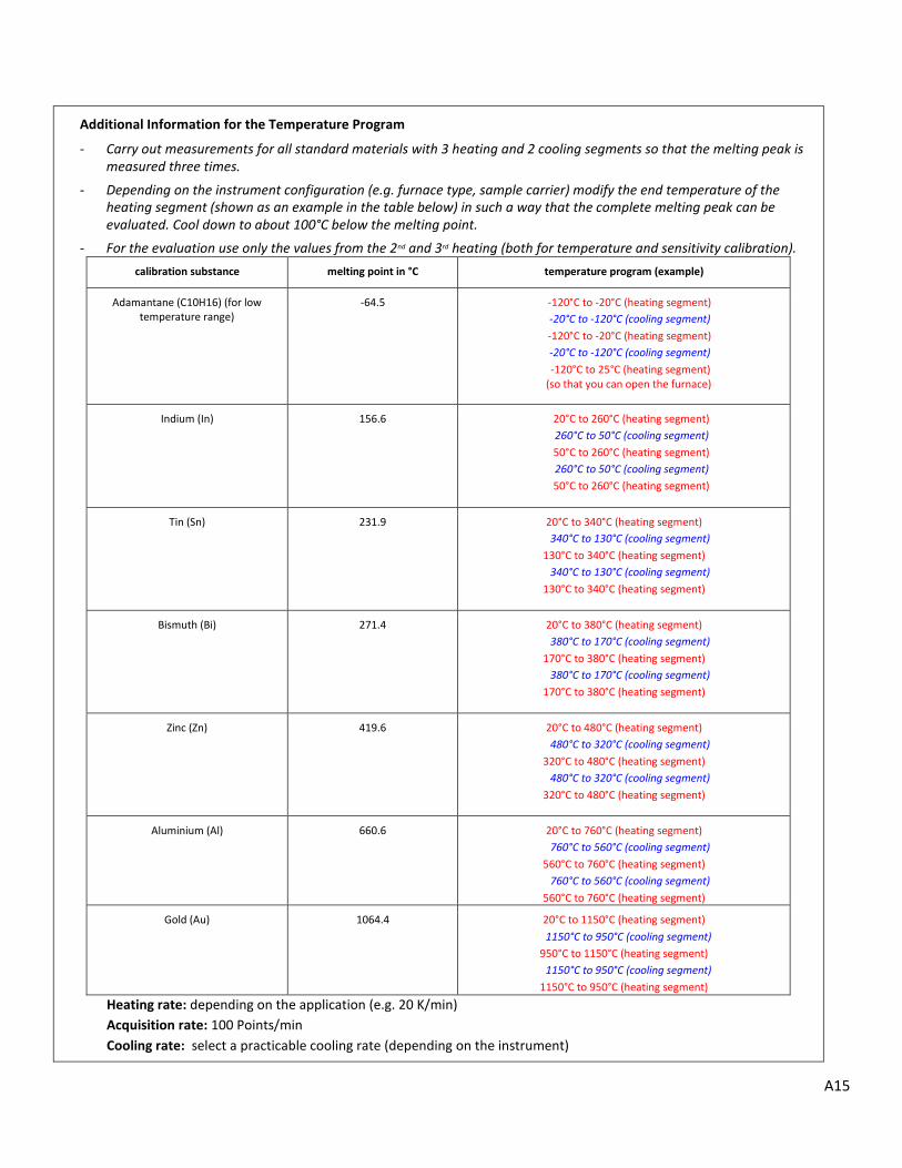
A15
Additional Information for the Temperature Program
- Carry out measurements for all standard materials with 3 heating and 2 cooling segments so that the melting peak is measured three times.
- Depending on the instrument configuration (e.g. furnace type, sample carrier) modify the end temperature of the heating segment (shown as an example in the table below) in such a way that the complete melting peak can be evaluated. Cool down to about 100°C below the melting point.
- For the evaluation use only the values from the 2nd and 3rd heating (both for temperature and sensitivity calibration).
calibration substance melting point in °C temperature program (example)
Adamantane (C10H16) (for low temperature range)
-64.5 -120°C to -20°C (heating segment) -20°C to -120°C (cooling segment) -120°C to -20°C (heating segment) -20°C to -120°C (cooling segment) -120°C to 25°C (heating segment)
(so that you can open the furnace)
Indium (In) 156.6 20°C to 260°C (heating segment) 260°C to 50°C (cooling segment) 50°C to 260°C (heating segment) 260°C to 50°C (cooling segment) 50°C to 260°C (heating segment)
Tin (Sn) 231.9 20°C to 340°C (heating segment) 340°C to 130°C (cooling segment)
130°C to 340°C (heating segment) 340°C to 130°C (cooling segment)
130°C to 340°C (heating segment)
Bismuth (Bi) 271.4 20°C to 380°C (heating segment) 380°C to 170°C (cooling segment)
170°C to 380°C (heating segment) 380°C to 170°C (cooling segment)
170°C to 380°C (heating segment)
Zinc (Zn) 419.6 20°C to 480°C (heating segment) 480°C to 320°C (cooling segment)
320°C to 480°C (heating segment) 480°C to 320°C (cooling segment)
320°C to 480°C (heating segment)
Aluminium (Al) 660.6 20°C to 760°C (heating segment) 760°C to 560°C (cooling segment)
560°C to 760°C (heating segment) 760°C to 560°C (cooling segment)
560°C to 760°C (heating segment)
Gold (Au) 1064.4 20°C to 1150°C (heating segment) 1150°C to 950°C (cooling segment)
950°C to 1150°C (heating segment) 1150°C to 950°C (cooling segment)
1150°C to 950°C (heating segment) Heating rate: depending on the application (e.g. 20 K/min) Acquisition rate: 100 Points/min
Cooling rate: select a practicable cooling rate (depending on the instrument)

A16
2. Evaluation of the Measurements
10. Open the Proteus Analysis.
11. Select Open in the File menu.
12. Open your respective measurement (the measurement file which you have saved under item 7).
Continue with Open.

A17
13. Select X-Temperature in the Settings menu. The temperature is shown on the X axis.
Temperature Calibration
14. Click on the DSC curve for selection. Select Onset in the Evaluation menu to determine the extrapolated onset.
15. To evaluate the extrapolated onset, define the right and left evaluation limit as shown in the figure and click Apply.
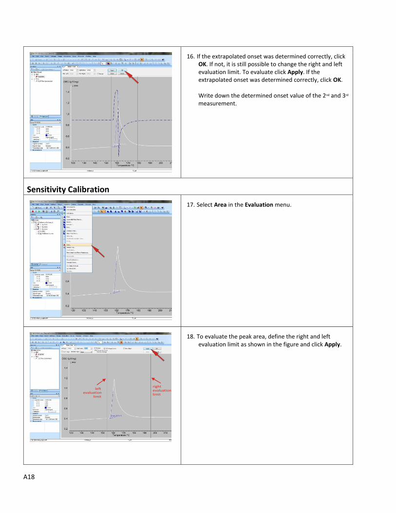
A18
16. If the extrapolated onset was determined correctly, click OK. If not, it is still possible to change the right and left evaluation limit. To evaluate click Apply. If the extrapolated onset was determined correctly, click OK.
Write down the determined onset value of the 2nd and 3rd measurement.
Sensitivity Calibration
17. Select Area in the Evaluation menu.
18. To evaluate the peak area, define the right and left evaluation limit as shown in the figure and click Apply.

A19
19. If the peak area was determined correctly, click OK. If not, it is still possible to change the right and left evaluation limit. To evaluate click Apply. If the peak area was determined correctly, click OK.
Write down the determined peak area of the 2nd and 3rd measurement.

A20
3. Creation of a Temperature/Sensitivity Calibration File
Temperature Calibration
20. Open Temperature Calibration in the NETZSCH-Proteus group.
21. Open Select Instrument in the File menu.
22. Select your instrument and click OK.

A21
23. Select New in the File menu.
24. Check the instrument configuration (change if necessary).
Continue with OK.
25. Define both the atmosphere and the heating rate used for the calibration measurements.
Continue with OK.
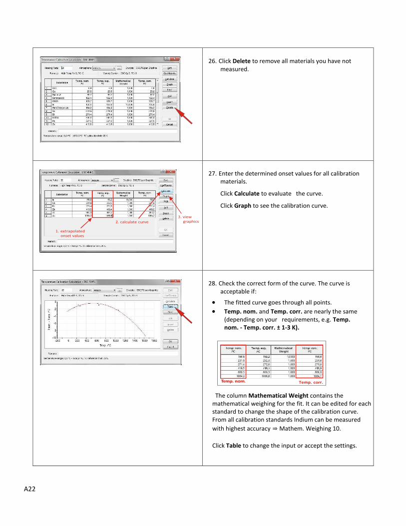
A22
26. Click Delete to remove all materials you have not measured.
27. Enter the determined onset values for all calibration materials.
Click Calculate to evaluate the curve.
Click Graph to see the calibration curve.
28. Check the correct form of the curve. The curve is acceptable if:
• The fitted curve goes through all points. • Temp. nom. and Temp. corr. are nearly the same
(depending on your requirements, e.g. Temp. nom. - Temp. corr. ± 1-3 K).
The column Mathematical Weight contains the mathematical weighing for the fit. It can be edited for each standard to change the shape of the calibration curve. From all calibration standards Indium can be measured
with highest accuracy ⇒ Mathem. Weighing 10. Click Table to change the input or accept the settings.

A23
29. Click OK to save the calculation.
30. Select Save as in the File menu to save the data.
31. Define the file name of the temperature calibration file and click Save.
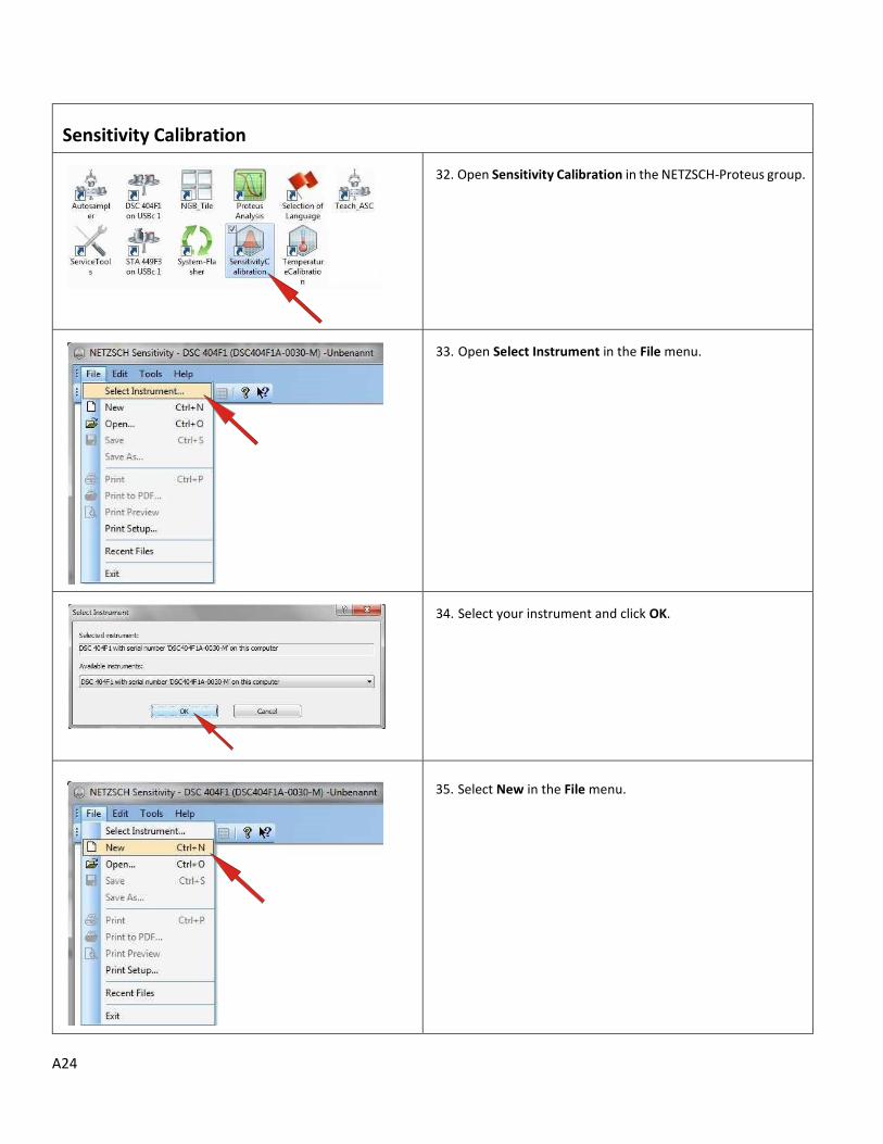
A24
Sensitivity Calibration
32. Open Sensitivity Calibration in the NETZSCH-Proteus group.
33. Open Select Instrument in the File menu.
34. Select your instrument and click OK.
35. Select New in the File menu.
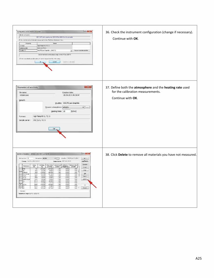
A25
36. Check the instrument configuration (change if necessary).
Continue with OK.
37. Define both the atmosphere and the heating rate used for the calibration measurements.
Continue with OK.
38. Click Delete to remove all materials you have not measured.
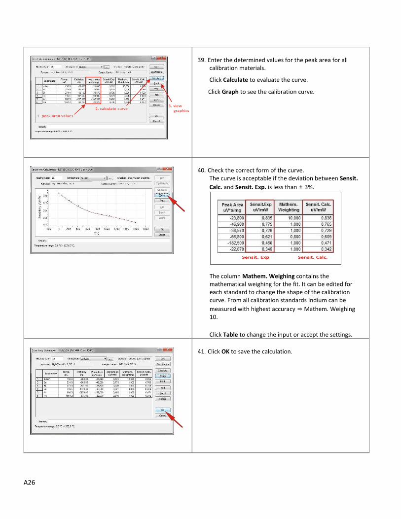
A26
39. Enter the determined values for the peak area for all calibration materials.
Click Calculate to evaluate the curve.
Click Graph to see the calibration curve.
40. Check the correct form of the curve. The curve is acceptable if the deviation between Sensit.
Calc. and Sensit. Exp. is less than ± 3%.
The column Mathem. Weighing contains the mathematical weighing for the fit. It can be edited for each standard to change the shape of the calibration curve. From all calibration standards Indium can be
measured with highest accuracy ⇒ Mathem. Weighing 10.
Click Table to change the input or accept the settings.
41. Click OK to save the calculation.
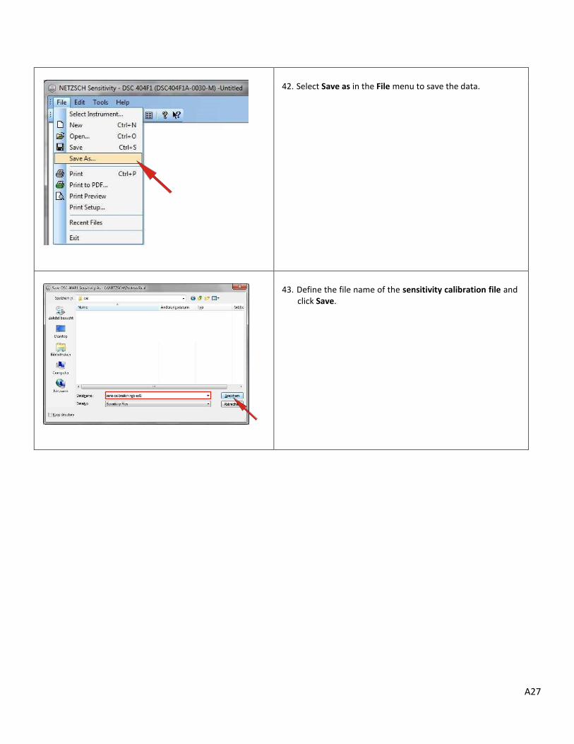
A27
42. Select Save as in the File menu to save the data.
43. Define the file name of the sensitivity calibration file and click Save.