Network mapping and optimization

Mapping and OptimisationBased on Australia National Broadband Network Design Rule

By

JIANLI MA, CHENG LIN, HAOZHENG WEI, CHIEN-CHENG LAI

Melbourne School of EngineeringUNIVERSITY OF MELBOURNE

OCTOBER 2014

Created by LATEX

EXECUTIVE SUMMARY

The project regards the National Broadband Network (NBN) Corporation as a reference fornetwork deployment of Fibre To The Premises (FTTP) by Google Map API with JavaScriptin urban, suburban areas. The algorithm includes Travelling Sales Man (TSP) and min-

imum spanning tree in order to find minimum distances among FDH, splitters and end users.The cost optimisation is also based on the Gigabit Passive Optical Network (GPON) structurewith a 1:32 splitter design to each end user premise. By using Google Map API, each premise willbe found following by FTTH deployment to meet NBN requirements. The structure of this projectis illustrated in Figure 1.

FIGURE 1. Mapping and Optimization1

In the project, the brief background will be provided following by optimisation of constructionand algorithms. After implementation of design via Google Map API, the conclusion is presentedat the end.

i

TABLE OF CONTENTS

Page

List of Figures v

1 Background 11.1 Introduction of FTTH Architecture . . . . . . . . . . . . . . . . . . . . . . . . . . . . . 11.2 DFN . . . . . . . . . . . . . . . . . . . . . . . . . . . . . . . . . . . . . . . . . . . . . . . 11.3 LFN . . . . . . . . . . . . . . . . . . . . . . . . . . . . . . . . . . . . . . . . . . . . . . . 21.4 Construction Optimization . . . . . . . . . . . . . . . . . . . . . . . . . . . . . . . . . . 3

2 Optimisation 52.1 DFN Optimisation . . . . . . . . . . . . . . . . . . . . . . . . . . . . . . . . . . . . . . . 52.2 LFN Optimisation . . . . . . . . . . . . . . . . . . . . . . . . . . . . . . . . . . . . . . . 52.3 Conclusion . . . . . . . . . . . . . . . . . . . . . . . . . . . . . . . . . . . . . . . . . . . 6

3 Design 73.1 Retrieving Geography Data and Data Pre-processing . . . . . . . . . . . . . . . . . . 73.2 Analysis Residency Data(Fibre Access Point) . . . . . . . . . . . . . . . . . . . . . . . 73.3 Automatic Layout . . . . . . . . . . . . . . . . . . . . . . . . . . . . . . . . . . . . . . . 8

3.3.1 Suburban Areas . . . . . . . . . . . . . . . . . . . . . . . . . . . . . . . . . . . 93.3.2 CBD Areas . . . . . . . . . . . . . . . . . . . . . . . . . . . . . . . . . . . . . . . 10

3.4 Visualisation . . . . . . . . . . . . . . . . . . . . . . . . . . . . . . . . . . . . . . . . . . 10

4 Suburban Area Example 114.1 Suburb One . . . . . . . . . . . . . . . . . . . . . . . . . . . . . . . . . . . . . . . . . . . 11

4.1.1 Data Collection . . . . . . . . . . . . . . . . . . . . . . . . . . . . . . . . . . . . 114.1.2 Data Processing . . . . . . . . . . . . . . . . . . . . . . . . . . . . . . . . . . . 114.1.3 Spanning Tree Layout . . . . . . . . . . . . . . . . . . . . . . . . . . . . . . . . 12

4.2 Suburb Two . . . . . . . . . . . . . . . . . . . . . . . . . . . . . . . . . . . . . . . . . . . 124.2.1 Data Collection . . . . . . . . . . . . . . . . . . . . . . . . . . . . . . . . . . . . 124.2.2 Data Processing . . . . . . . . . . . . . . . . . . . . . . . . . . . . . . . . . . . 134.2.3 Spanning Tree Layout . . . . . . . . . . . . . . . . . . . . . . . . . . . . . . . . 13

iii

TABLE OF CONTENTS

4.2.4 Optimisation . . . . . . . . . . . . . . . . . . . . . . . . . . . . . . . . . . . . . 13

5 CBD Area Example 235.1 Data Collection . . . . . . . . . . . . . . . . . . . . . . . . . . . . . . . . . . . . . . . . . 235.2 Data Processing . . . . . . . . . . . . . . . . . . . . . . . . . . . . . . . . . . . . . . . . 235.3 Visualisation . . . . . . . . . . . . . . . . . . . . . . . . . . . . . . . . . . . . . . . . . . 24

6 Conclusion 27

A Maps Data Retrieving and Processing Program 29

A Suburban Area Layout Program 35

A CBD Area Layout Program 39

A Contribution Table 47

A Gantt Chart for Mapping and Optimization 49

Bibliography 51

iv

LIST OF FIGURES

1 Mapping and Optimization . . . . . . . . . . . . . . . . . . . . . . . . . . . . . . . . . . . . iFIGURE Page

1.1 The passive optical network architecture of FTTH deployment. . . . . . . . . . . . . . . 21.2 GPON Standard . . . . . . . . . . . . . . . . . . . . . . . . . . . . . . . . . . . . . . . . . . 21.3 FASM with 16 FDAs. . . . . . . . . . . . . . . . . . . . . . . . . . . . . . . . . . . . . . . . 31.4 Hierarchical Components in LFN . . . . . . . . . . . . . . . . . . . . . . . . . . . . . . . . 41.5 Comparison of 2011-13 Corporate Plan vs. 2012-15 Corporate Plan for the Fibre Network 4

3.1 FlowChart of Addresses Acquiring . . . . . . . . . . . . . . . . . . . . . . . . . . . . . . . 83.2 FlowChart of Data Processing . . . . . . . . . . . . . . . . . . . . . . . . . . . . . . . . . . 9

4.1 Original Map in Sub 1 . . . . . . . . . . . . . . . . . . . . . . . . . . . . . . . . . . . . . . 124.2 Residential Premises in Sub 1 . . . . . . . . . . . . . . . . . . . . . . . . . . . . . . . . . . 134.3 Residential Premises in Sub 1 . . . . . . . . . . . . . . . . . . . . . . . . . . . . . . . . . . 144.4 Coordinates of Access Points . . . . . . . . . . . . . . . . . . . . . . . . . . . . . . . . . . . 144.5 Distances between Access Points and Exchange Centre. . . . . . . . . . . . . . . . . . . 154.6 Distances between Access Points and Exchange Centre. . . . . . . . . . . . . . . . . . . 154.7 Spanning Tree Result . . . . . . . . . . . . . . . . . . . . . . . . . . . . . . . . . . . . . . . 164.8 Visualisation of Spanning Tree Result . . . . . . . . . . . . . . . . . . . . . . . . . . . . . 164.9 Optimisation Result . . . . . . . . . . . . . . . . . . . . . . . . . . . . . . . . . . . . . . . . 174.10 Original Map in Sub 2 . . . . . . . . . . . . . . . . . . . . . . . . . . . . . . . . . . . . . . 174.11 Residential Premises in Sub 2 . . . . . . . . . . . . . . . . . . . . . . . . . . . . . . . . . . 184.12 Residential Premises in Sub 2 . . . . . . . . . . . . . . . . . . . . . . . . . . . . . . . . . . 184.13 Coordinates of Access Points . . . . . . . . . . . . . . . . . . . . . . . . . . . . . . . . . . . 194.14 Distances between Access Points and Exchange Centre. . . . . . . . . . . . . . . . . . . 194.15 Distances between Access Points and Exchange Centre. . . . . . . . . . . . . . . . . . . 204.16 Spanning Tree Result . . . . . . . . . . . . . . . . . . . . . . . . . . . . . . . . . . . . . . . 204.17 Visualisation of Spanning Tree Result . . . . . . . . . . . . . . . . . . . . . . . . . . . . . 214.18 Optimisation Result . . . . . . . . . . . . . . . . . . . . . . . . . . . . . . . . . . . . . . . . 21

5.1 Original Map in CBD . . . . . . . . . . . . . . . . . . . . . . . . . . . . . . . . . . . . . . . 24

v

LIST OF FIGURES

5.2 Commercial Premises in CBD . . . . . . . . . . . . . . . . . . . . . . . . . . . . . . . . . . 255.3 TSP Solution . . . . . . . . . . . . . . . . . . . . . . . . . . . . . . . . . . . . . . . . . . . . 255.4 TSP Solution . . . . . . . . . . . . . . . . . . . . . . . . . . . . . . . . . . . . . . . . . . . . 26

vi

CH

AP

TE

R

1BACKGROUND

Delivering fibre to the end user premises dominates 93% of the NBN Co access network[4].The access network consists of distribution fibre network (DFN) and local fibre net-work(LFN).

1.1 Introduction of FTTH Architecture

The project utilises home run architecture of FTTH that dedicated fibres connect each home tothe point of presence (POP). A Remote Node (RN) is deployed between the POP and the user’spremises and they do not have any active electronics. A passive splitter at the RN deliversthe downstream optical messages from the feeder fibre to the individual distribution fibre. Thepassive optical network architecture of FTTH deployment is shown in Figure 1.1. The feature isthat passive optical splitters distribute the fibre to each end user with splitting ratios 1:32 asGPON architecture in our project.The standard of GPON is summarised in Figure 1.2. This shows that bandwidths bit rates in

upstream and downstream are shared by 16, 32, 64 or 128 users depending on the requirementsof deployment. According to NBN Co, GPON is the most cost-effective approach for higherdownstream bit rates and lower overhead than other PON architectures.

1.2 DFN

DFN is used to connect fibre access node(FAN) located at central office and fibre distributionhubs(FDHs) located at the street side cabinets with ribbon fibre core needed between 288 to 864fibres, but preferred 576[7]. It could be shown in Figure 1.3. Maximum 16 FDHs can be connectedto one FAN in the fibre serving area module(FSAM) with loop topology, starting from a FAN site

1

CHAPTER 1. BACKGROUND

FIGURE 1.1. The passive optical network architecture of FTTH deployment.

FIGURE 1.2. GPON Standard

and finishing at the same site. Each FDH located at one fibre distribution area(FDA) can serve200 premises on average.

1.3 LFN

LFN is used to connect FDH and end user premises in start topology with 1:32 passive splitter,or in a P2P topology with direct connection. The underground deployment LFN is composed oflocal network splice and multi-port located at the pits, which is indicated in Figure 1.4.[3]

2

1.4. CONSTRUCTION OPTIMIZATION

FIGURE 1.3. FASM with 16 FDAs.[7]

1.4 Construction Optimization

As can be seen from Figure 1.5, the 2012-15 Corporate Plan forecasts a net increase ($1.4 billionand $3.2 billion respectively) in Capital Expenditure and Operating Expenditure during theFibre Network Construction period to FY2021. And one of the reasons is due to the implicationsof the Government’s New Developments policy.[9][2]

In order to keep undesired growth of expenditure under an acceptable level, strategies must beimplemented to optimise the construction cost. For example, optimising the trench paths of dropfibres and allocation of pits following the existing civil infrastructure and network.[1]

However, all the methods have to refer to the latest NBN Co Network Design Rules.

3

FIGURE 1.4. Hierarchical Components in LFN.[6]

FIGURE 1.5. Comparison of 2011-13 Corporate Plan vs. 2012-15 Corporate Plan for theFibre Network

CH

AP

TE

R

2OPTIMISATION

Since NBN Co divides access network into two parts, DFN in a loop topology and LFNin a star topology. In this section, two optimisation methods are used to DFN and LFNrespectively.

2.1 DFN Optimisation

Constraints of the NBN Co DFN network:1. The distance between FAN and the farthest FDH is 4km2. Fibre core counts should be between 288 to 864 fibres3. Maximum 16 FDAs connects to one FAN.

The Travelling Salesman Problem(TSP) algorithm is used for DFN optimisation to make theshortest loop between FAN and FDHs, so that the cost mainly on civil work can be saved asmuch as possible. Branch and Bound algorithm as one of the TSP method is chosen to design thedistribution network in this project under the constraints of NBN Co network.

2.2 LFN Optimisation

Constraints of the NBN Co LFN network:1. Fibre core counts between 72 to 288 fibres2. On average of 200 premises can be served by one FDH3. Residential users in SDU or MDU should be provided with 1.5 fibres for each premise4. Commercial MDU should be served by 2 fibres for each premises.

5

CHAPTER 2. OPTIMISATION

Minimum Spanning Tree(MST) algorithm is used to optimise the LFN in suburb. Consider-ing the constraints defined by NBN Co, 20 premises in suburb area are served by one 1:32 splitterto guarantee 1.5 fibres connection. In order to serve 200 end users in one FDA, 18 splittersare needed for splitting cable with 576 core count fibres. MST algorithm is used to connect allsplitters with minimum path and avoid loop connection to achieve cost optimisation.[5]

2.3 Conclusion

In CBD areas, the premises are usually in demand of high throughput and availability. With theaccount of incomes resulted from the high population density, the heavy investment in this areacould be shouldered by ISP. Therefore, P2P topology is used to connect FAN to CBD and followedby TSP algorithm. While TSP algorithm and MST are implemented for DFN and LFN in suburbrespectively.[8]

6

CH

AP

TE

R

3DESIGN

In this part, the description of coding part and related algorithm are included. This partwould be discussed by dividing into four sections: 1. Retrieving geography data; 2. AnalysisResidency Data(Fibre Access Point); 3. Automatic Layout; 4. Visualisation.

3.1 Retrieving Geography Data and Data Pre-processing

Google Maps is used to acquire the map data, which provides API for developers. For privacyconsideration, Google Maps API does not provide the accuracy coordinate for every residentialaddresses.[13] Therefore, a traversal method to recognise the addresses and acquire their coordi-nates. To be detailed, after an area is selected in the map, a traversal robot would be triggeredfrom the top-left corner to bottom-right corner to test every point. For each point, the robot wouldrequest its address information through Google Maps API and recorded it with the correspondcoordinate of this point in its database. After all the points in this area have been scanned, therobot would delete the items with the same addresses and calculate the mean coordinates ofthese addresses. The Figure 3.1 reveals this processing.[10][11]

3.2 Analysis Residency Data(Fibre Access Point)

After doing it, these raw data will be processed, and for convenience, all of absolute coordinatesto the relative coordinates are transformed. The practical method is setting the top-left corner as(0,0) while the bottom-right corner has a new coordinate of (1600,1600)(As we always require asquare area). Then a matrix recorded all the residential places with their relative coordinates isrecorded. The Figure 3.2 illustrates the acquiring processes in suburban areas.[12]

7

CHAPTER 3. DESIGN

Select Location Range

Within Australia?

Fetch the Centre Coordinate

Read the Square Corner Coordinates

Generate 1600*1600 Matrix

Fill the Matrix with Coordinates

Ask the Address of the nth Element

n<1600*1600?

Y

N

The Response Address is Repeated?

Record this Group

n=n+1

Y

Y

END

N

N

FIGURE 3.1. FlowChart of Addresses Acquiring

3.3 Automatic Layout

According to the different geography characters, this problems could be considered in two cate-gories of circumstances, separately.

8

3.3. AUTOMATIC LAYOUT

Read the Raw Data

Divide the Points into 16 Groups According to Their Coordinates

Divide the Points into 16 Groups According to Their Coordinates

Divide the nth Small Group into 4*4 Grip

n<16?

Count which Grid Contains the Most Addresses

Set this Point as the Location of Splitter

Create a 17*17 2-Dimension Matrix

N

Record the Splitter Coordinates

n=n+1

Calculate the Distances Between Any Two Elements

Output Results

FIGURE 3.2. FlowChart of Data Processing

3.3.1 Suburban Areas

For suburban areas, the destiny of population is not very high and pretty average on distribution.A method of "Central Office + Splitter" is thus adopted. And the layout problem is transformedinto a spanning tree optimisation problem. Specifically, the splitter positions are calculated

9

CHAPTER 3. DESIGN

initially. According to the distribution of Users’ Premises, the principle that splitters are alwaysset in the areas where most of the premises locate is adopted. Therefore, we create a two-layersstructure to finish this algorithm. The first layer divides the area into 16 small areas whichmeans there would be 16 splitters in this district. Then, a further 16-cells grid would be put overthe first layer to identify the location of splitter in this area.

3.3.2 CBD Areas

In terms of CBD areas, the subscribers are dominated by business users which require highthroughputs and reliability. Consequently, the "Loop Access" method will be utilised as it canprovide not only a redundant access guarantee but also improve the bandwidth between localbusiness users. The problem becomes a Travelling Salesman Problem(TSP).

3.4 Visualisation

Then the data would be processed again which involves transformation from relative coordinatesto absolute coordinates before visualisation. According to the absolute coordinates of linkingnodes, the solution is re-drawn on the map.

10

CH

AP

TE

R

4SUBURBAN AREA EXAMPLE

Suburban areas comprise the majority spaces of Australia. Therefore the discussion ofcoverage, layout and optimisation work in suburbs is essential. In this chapter, twoinstances are presented, which one of them is a low-population destiny residential area

while the other one is a common community. The explanation of algorithm running with analysisand results would be given step-by-step.

4.1 Suburb One

This area is selected randomly where located in the eastern of Melbourne Metropolis.Figure 4.1is the original map retrieving from Google Maps.

4.1.1 Data Collection

Google Maps API is used to collect the geography data for the following analysis. As describedbefore, our program could acquire the addresses of every residential premises in this area. Andthe raw data is presented in Figure 4.2.

4.1.2 Data Processing

Then the Access Point is selected based on these residential premises. Figure 4.3 illustrates thelocations of Access Points.

Figure 4.4 illustrates the coordinates of Access Points.

11

CHAPTER 4. SUBURBAN AREA EXAMPLE

FIGURE 4.1. Original Map in Sub 1

Figure 4.5 and Figure 4.6 illustrate the distances between Access Points and Exchange Centre.

4.1.3 Spanning Tree Layout

Then, the Prim Algorithm is used to calculate the minimum spanning tree. The result output isshown in Figure 4.7 and the visualisation result is shown in Figure 4.8.

4.2 Suburb Two

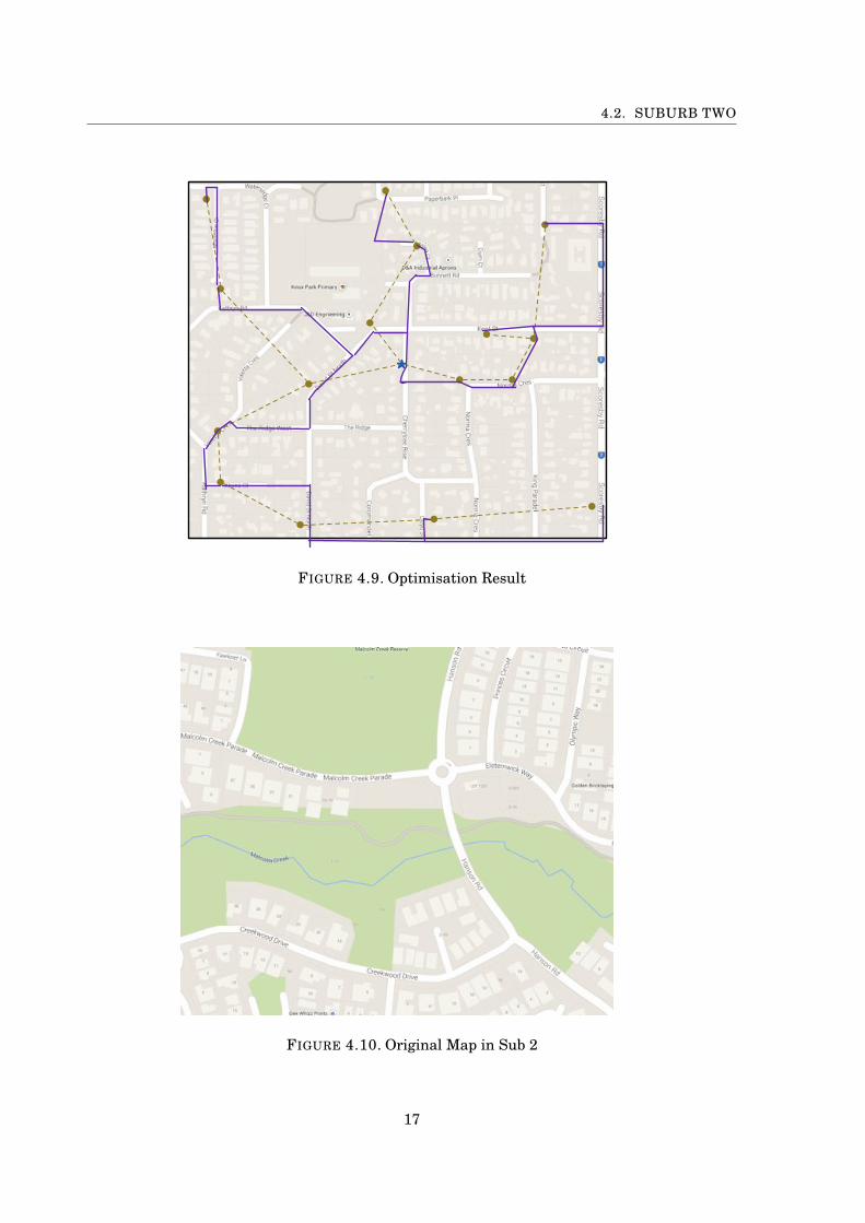
This area is selected randomly where located in the northern of Melbourne Metropolis.Figure 4.10is the original map retrieving from Google Maps.

4.2.1 Data Collection

Google Maps API is used to collect the geography data for the following analysis. As describedbefore, our program could acquire the addresses of every residential premises in this area. Andthe raw data is presented in Figure 4.11.

12

4.2. SUBURB TWO

FIGURE 4.2. Residential Premises in Sub 1

4.2.2 Data Processing

Then the Access Point is selected based on these residential premises. Figure 4.12 illustrates thelocations of Access Points.

Figure 4.13 illustrates the coordinates of Access Points.Figure 4.14 and Figure 4.15 illustrate the distances between Access Points and Exchange

Centre.

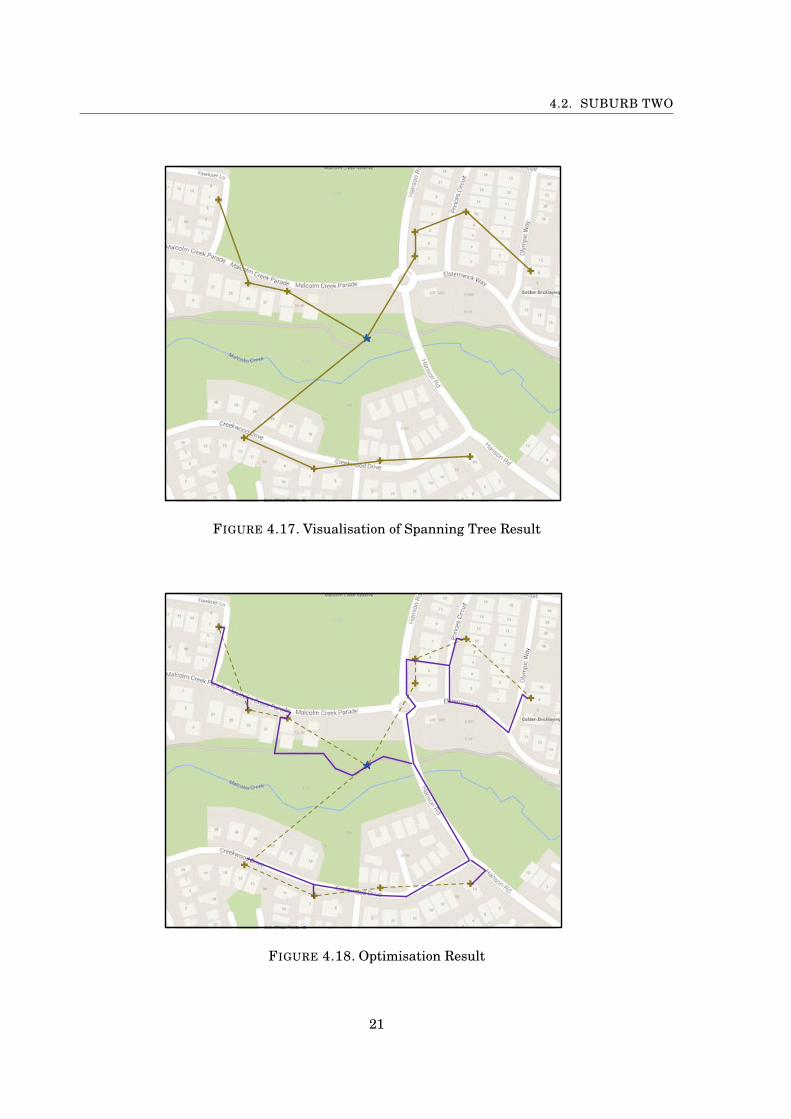
4.2.3 Spanning Tree Layout

Then, Prim Algorithm is used to calculate the minimum spanning tree. The result output isshown in Figure 4.16 and the visualisation result is shown in Figure 4.17.

4.2.4 Optimisation

13


FIGURE 4.4. Coordinates of Access Points

4.2. SUBURB TWO

FIGURE 4.5. Distances between Access Points and Exchange Centre.


15


FIGURE 4.7. Spanning Tree Result

FIGURE 4.8. Visualisation of Spanning Tree Result

16

4.2. SUBURB TWO

FIGURE 4.9. Optimisation Result

FIGURE 4.10. Original Map in Sub 2

17




18

4.2. SUBURB TWO

FIGURE 4.13. Coordinates of Access Points


19



FIGURE 4.16. Spanning Tree Result

20

4.2. SUBURB TWO

FIGURE 4.17. Visualisation of Spanning Tree Result

FIGURE 4.18. Optimisation Result

21

CH

AP

TE

R

5CBD AREA EXAMPLE

Comparing with manual method to find optimising trench paths, program in this projecthelps operators save CAPEX which may include expensive labour cost, save processingtime consumed, and avoid human error. The second feature of this project is that the

highly reliable program is flexible at other locations under the constraints of NBN Co networkdesign rules. Another important part of this program is that it works with Google Map API toprovide friendly visualise result in real scenarios.

Because it takes some time to run TSP algorithm for an optimal solution when the numberof nodes is too much. However, the program could be optimised with longer developing time.Therefore, the program is expected to be used within a limit number of nodes in CBD and DFN.

Being similar to the processing steps of suburban areas, the first step is to retrieve thegeography data by Google Maps API.Figure 5.1 is the original map retrieving from Google Maps.

5.1 Data Collection

Google Maps API is used to collect the geography data for the following analysis. In CBD areas,the residential addresses are rarely and the commercial premises attract more attention in termsof layout. Figure 5.2 illustrates the location information in CBD Areas.

5.2 Data Processing

To build up a network in CBD Area, the loop layout method is adopted as the reliability is put inthe priority. Then the layout and optimisation problem is converted to a TSP. The solution of this

23

CHAPTER 5. CBD AREA EXAMPLE

FIGURE 5.1. Original Map in CBD

area is shown in Figure 5.3

5.3 Visualisation

In the end, the solution would be put back on the maps again to make this solution obviously.

24

FIGURE 5.2. Commercial Premises in CBD

FIGURE 5.3. TSP Solution

CHAPTER 5. CBD AREA EXAMPLE

FIGURE 5.4. TSP Solution

26

CH

AP

TE

R

6CONCLUSION

The project aims to propose a FTTH GPON network, covering real nodes (premises) in-cluded CBD and suburban areas under the constraint of NBN Co rules for the deploymentby implementing TSP and MST algorithms on Google Map API.

Comparing with manual method to find optimising trench paths, program in this project helpsoperators save CAPEX which may include expensive labour cost, save processing time consumed,and avoid human error. The second feature of this project is that the highly reliable programis flexible at other locations under the constraints of NBN Co network design rules. Anotherimportant part of this program is that it works with Google Map API to provide friendly visualiseresult in real scenarios.

Because it takes some time to run TSP algorithm for an optimal solution when the numberof nodes is too much. However, the program could be optimised with longer developing time.Therefore, the program is expected to be used within a limit number of nodes in CBD and DFN.

27

AP

PE

ND

IX

AMAPS DATA RETRIEVING AND PROCESSING PROGRAM

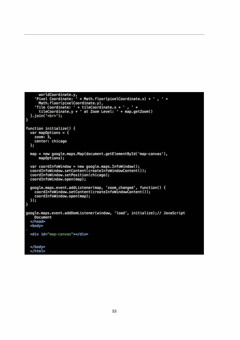
This is the source code of Maps Data Retrieving and Processing Program.

The aim of this program is retrieve the geography data from selected area and analysis thepremises in this area. This program is coded in HTML+JavaScript.The input is coordinates of a certain area which the operator could drag the rectangle selector inthe webpage to select. The output is a matrix recorded all the addresses coordinates in a relativedistance.(i.e. The maximum coordinates in the area is 1600£1600.)

29

APPENDIX A. MAPS DATA RETRIEVING AND PROCESSING PROGRAM

30

AP

PE

ND

IX

ASUBURBAN AREA LAYOUT PROGRAM

This is the source code of Suburban Area Layout Program in Matlab programming lan-guage.

The aim of this program is to read the geography data from the output of Program 1 and givethe layout solution.The input is the coordinates matrix which is generated from Program 1. Then the input areawould be divided into 16 areas. According to the destiny of population, the optimum splitterwould be selected and put in a spot which is the distance between them is calculated and recordedthen. After that, the layout problem has been converted into a spanning tree problem and thesolution would be given to generate the minimum spanning tree.

35

AP

PE

ND

IX

ACBD AREA LAYOUT PROGRAM

This is the source code of CBD Area Layout Program in Matlab programming language.

The aim of this program is to read the geography data from the output of Program 1 and givethe layout solution.The input is the coordinates matrix which is generated from Program 1. Then the mutual dis-tances of all the commercial addresses would be calculated and recorded. As the requirement of aloop structure, the TSP solution would be implemented and the final result would be given.

39

APPENDIX A. CBD AREA LAYOUT PROGRAM

40


42


44

AP

PE

ND

IX

ACONTRIBUTION TABLE

47

AP

PE

ND

IX

AGANTT CHART FOR MAPPING AND OPTIMIZATION

49

BIBLIOGRAPHY

[1] Fiber to the home primers(august 2013 premier).

[2] Fiber to the home(what fiber can do for australia).

[3] National broadband network a user’s perspective.

[4] Nbn co.,network design rule, 19th December 2011.

[5] Nbn co.,corporate plan, 2012-2015.

[6] Nbn co.,nbn co new development: Deployment of the nbn, 9th July 2013.

[7] Nbn co.,network design rule, 1st July 2014.

[8] S. AZODOLMOLKY AND I. TOMKOS, A techno-economic study for active ethernet ftth deploy-

ments., Journal of Telecommunications Management, 1 (2008), pp. 294 – 310.

[9] N. CO., The australian national broadband network: New opportunities, new challenges.

[10] D. GOSNELL, Professional Web APIs [electronic resource] : Google, eBay, Amazon.com,

MapPoint, FedEx / Denise Gosnell., Indianapolis, Ind. ; [Great Britain] : Wiley, c2005.,2005.

[11] G. SVENNERBERG, Beginning Google Maps API 3 [electronic resource] / Gabriel Svenner-

berg., Expert’s voice in Web development, [New York] : Apress, c2010., 2010.

[12] T. R. WEISS, Google developers get revamped google api console to manage apis., eWeek,(2013), p. 6.

[13] Z. YING, Introducing google chart tools and google maps api in data visualization courses.,IEEE Computer Graphics and Applications, (2012), p. 6.

51

Network mapping and optimization

Documents

Transcript of Network mapping and optimization