“Network Growth Models”

MAE 298, Lecture 3April 6, 2006

“Network Growth Models”

Recall: Properties of Erdos-Renyi random graphs:

1. Phase transition in connectivity at average node degree, z = 1(i.e., p = 1/n).

2. Poisson degree distribution, pk = zke−z/k!.

3. Diameter, d ∼ log N , a small-world network.

4. Clustering coefficient; none.

Properties (1) and (3) are in-line with real-world networks, butnot properties (2) and (4).

Degree distribution

• A large number of real-world networks, from an extensiverange of applications, have “heavy-tailed” degree distributions.

• Also can be considered “broad-scale”.

• The simplest example of such a distribution is a power law.

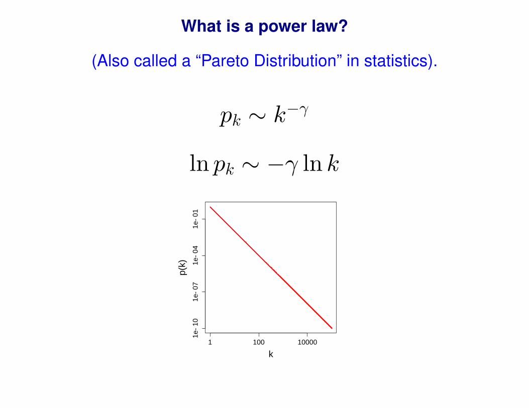
What is a power law?

(Also called a “Pareto Distribution” in statistics).

pk ∼ k−γ

ln pk ∼ −γ ln k

1 100 10000

1e−

101e

−07

1e−

041e

−01

k

p(k)

Properties of a power law distribution

See chalk board discussion. Essentially:

∫xn = 1

n+1 xn+1

Properties of a power law PDF (Summary)

(PDF = probability density function)

• To be a properly defined probability distribution need γ > 1.

• For 1 < γ ≤ 2, both the average 〈k〉 and standard deviation σ2

are infinite!

• For 2 < γ ≤ 3, average 〈k〉 is finite, but standard deviation σ2

is infinite!

• For γ > 3, both average and standard deviation finite.

Power laws in the real world

Confusion

• Power law

• Log normal

• Weibull

All three of these distributions can look the same! (Especiallywhen we are dealing with finite data sets — not enough data to

get good statistics).

How to deal with real data

• Can adjust bin size: increase exponentially with degree.

• Consider the Cumulative PDF (the CDF): Pk =∑∞

l=k pl.

For more details see:

• Newman Review, pages 12-13.

• Mitzenmacher Review (reference given at end).

But definitively observed in many systems

• Signature of a system at the “critical point” of a phasetransition.

• Random graphs at critical point;component sizes: Nk ∼ k−5/2

(Note, γ = 2.5)

1 2 5 10 20 50 100 200

110

100

1000

1000

0size, i

Ci

Ci = A * i−γ ; γ = 2.054247

Power laws in social systems

• Popularity of web pages: Nk ∼ k−1

• Rank of city sizes (“Zipf’s Law”): Nk ∼ k−1

• Pareto. In 1906, Pareto made the now famous observationthat twenty percent of the population owned eighty percentof the property in Italy, later generalised by Joseph M. Juranand others into the so-called Pareto principle (also termed the80-20 rule) and generalised further to the concept of a Paretodistribution.

• Usually explained in social systems by “the rich get richer”(preferential attachment).

Known Mechanisms for Power Laws

• Phase transitions (singularities)

• Random multiplicative processes (fragmentation)

• Combination of exponentials (e.g. word frequencies)

• Preferential attachment / Proportional attachment(Polya 1923, Yule 1925, Zipf 1949, Simon 1955, Price 1976,Barabasi and Albert 1999)

Attractiveness is proportional to size,

dP (s)dt ∝ s

Origins of preferential attachment

• 1923 — Polya, urn models.

• 1925 — Yule, explain genetic diversity.

• 1949 — Zipf, distribution of city sizes (1/f ).

• 1955 — Simon, distribution of wealth in economies. (“The richget richer”).

• [Interesting note, in sociology this is referred to as the Mattheweffect after the biblical edict, “For to every one that hath shallbe given ... ” (Matthew 25:29)]

Preferential attachment in networks

D. J. de S. Price: “Cumulative advantage”

• D. J. de S. Price, “Networks of scientific papers” Science, 1965.First observation of power laws in a network context.Studied paper co-citation network.

• D. J. de S. Price, “A general theory of bibliometric and othercumulative advantage processes” J. Amer. Soc. Info. Sci.,1976.

Cumulative advantage seemed like a natural explanation forpaper citations:

The rate at which a paper gains citations is proportional to thenumber it already has. (Probability to learn of a paperproportional to number of references it currently has).

Preferential attachment in networks, continued

Cumulative advantage did not gain traction at the time. But wasrediscovered some decades later by Barabasi and Albert, in the

now famous (about 1000 citations in SCI) paper:

“Emergence of Scaling in Random Networks”, Science 286,1999.

They coined the term “preferential attachment” to describe thephenomena.

The Barabasi and Albert model

• A discrete time process.

• Start with single isolated node.

• At each time step, a new node arrives.

• This node makes m connections to already existing nodes.(Why m edges?)

• We are interested in the limit of large graph size.

Probability

• Probability incoming node attaches to node j:

Pr(t + 1→ j) = dj/∑

j dj.

• Probability incoming node attaches to any node of of degree k:

(# nodes of degree k)/(# nodes) x (degree of that node)/(degree sum over all nodes) =

kpk∑k dk

= kpk2mn

Network evolutionProcess on the degree sequence

• Note that pk will change in time!So we show denote this explicitly: pk,t

• Also, when a node of degree k gains an attachment, itbecomes a node of degree k + 1.

• When the new node arrives, it increases by one the number ofnodes of degree m.

Markov flow

0 1 3 4 A (A+1)2

Process on the degree sequence, cont.(Let nk,t ≡ number of nodes of degree k at time t,

and nt ≡ total number of nodes at time t: Note nt = t)

For each arriving link:

• For k > m : nk,t+1 = nk,t + (k−1)2mt nk−1,t − k

2mt nk,t

• For k = m : nm,t+1 = nm,t + 1− m2mt nm,t

But each arriving node contributes m links:

• For k > m : nk,t+1 = nk,t + m(k−1)2mt nk−1,t − mk

2mntnk,t

• For k = m : nm,t+1 = nm,t + 1− m2

2mt nm,t

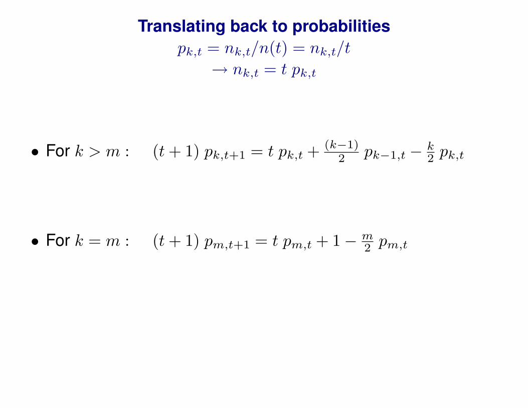
Translating back to probabilitiespk,t = nk,t/n(t) = nk,t/t

→ nk,t = t pk,t

• For k > m : (t + 1) pk,t+1 = t pk,t + (k−1)2 pk−1,t − k

2 pk,t

• For k = m : (t + 1) pm,t+1 = t pm,t + 1− m2 pm,t

Steady-state distribution

We want to consider the final, steady-state: pk,t = pk.

• For k > m : (t + 1) pk = t pk + (k−1)2 pk−1 − k

2 pk

• For k = m : (t + 1) pm = t pm + 1− m2 pm

Rearranging and solving for pk:

• For k > m : pk = (k−1)(k+2) pk−1

• For k = m : pm = 2(m+2)

Recursing to pm

pk = (k−1)(k−2)···(m)(k+2)(k+1)···(m+3) · pm = m(m+1)(m+2)

(k+2)(k+1)k ·2

(m+1)

pk = 2m(m+1)(k+2)(k+1)k

For k � 1

pk ∼ k−3

Did we prove the behavior of the degree distribution?

Details glossed over

1. Proof of convergence to steady-state

2. Proof of concentration (Need to show fluctuations in eachrealization small, so that the average nk describes well mostrealizations of the process).

– For this model, we can use the second-moment method(show that the effect of one different choice at time t dies outexponentially in time).

Issues

• Whether there are really true power-laws in networks? (Usuallyrequires huge systems, and no constraints on resources).

• Only get γ = 3!

Generalizations of Pref. Attach.

• Vary steps of P.A. with steps of random attachment.

• Consider non-linear P.A., where prob(attaching to node ofdegree k) ∼ (dk)b.

Simulating PA

Basic code for simulating PA with m = 1 using R:

• runPA← function(N=100){

# outLink[i] is the parent of ioutLink← numeric(N)# numlinks[i] is number total-links (in and out) for node inumLinks← numeric(N)+1for(i in 2:N){

p← sample(c(1:(i-1)),size=1,prob=numLinks[1:(i-1)])outLink[i]← pnumLinks[p]← numLinks[p]+1

}return(list(outLink, numLinks))

}

Visualizing a PA graph (m = 1) at n = 5000

Further reading:(All refs available on “references” tab of course web page)

PA model of network growth

• Barabasi and Albert, “Emergence of Scaling in RandomNetworks”, Science 286, 1999.

• B. Bollobas, O. Riordan, J. Spencer, and G. Tusnady, “Thedegree sequence of a scale-free random process”, RandomStructures and Algorithms 18(3), 279-290, 2001.


• Durrett Book, Chapter 4.

Further reading, cont.

Fitting power laws to data


• M. Mitzenmacher, “A Brief History of Generative Modelsfor Power Law and Lognormal Distributions”, InternetMathematics 1 (2), 226-251, 2003.

“Network Growth Models”

Documents

Transcript of “Network Growth Models”