Network Analyzer Basics - index-of.co.ukindex-of.co.uk/Tutorials/network_analyzer_basics.pdf ·...

Network Analyzer Basics



Network Analysis is NOT.…

RouterBridgeRepeater

Hub

Your IEEE 802.3 X.25 ISDN switched-packet data stream is running at 147 MBPS with a BER of 1.523 X 10 . . . -9


What Types of Devices are Tested?

Device type ActivePassive

Inte

grat

ion

High

Low

Antennas

SwitchesMultiplexersMixersSamplersMultipliers

Diodes

DuplexersDiplexersFiltersCouplersBridgesSplitters, dividersCombinersIsolatorsCirculatorsAttenuatorsAdaptersOpens, shorts, loadsDelay linesCablesTransmission linesWaveguideResonators

DielectricsR, L, C's

RFICsMMICsT/R modulesTransceivers

ReceiversTunersConverters

VCAsAmplifiers

VCOsVTFsOscillatorsModulatorsVCAtten’s

Transistors


Device Test Measurement Model

NF

Stimulus type ComplexSimple

Com

plex

Resp

onse

tool

Sim

ple

DC CW Swept Swept Noise 2-tone Multi- Complex Pulsed- Protocolfreq power tone modulation RF

Det/Scope

Param. An.

NF Mtr.

Imped. An.

Power Mtr.

SNA

VNA

SA

VSA

84000

TG/SA

Ded. Testers

I-V

Absol. Power

Gain/Flatness

LCR/Z

Harm. Dist.LO stabilityImage Rej.

Gain/Flat.Phase/GDIsolationRtn Ls/VSWRImpedanceS-parameters

Compr'nAM-PM

RFIC test

Full call sequence

Pulsed S-parm.Pulse profiling

BEREVMACP

RegrowthConstell.

Eye

IntermodulationDistortionNF

Measurement plane


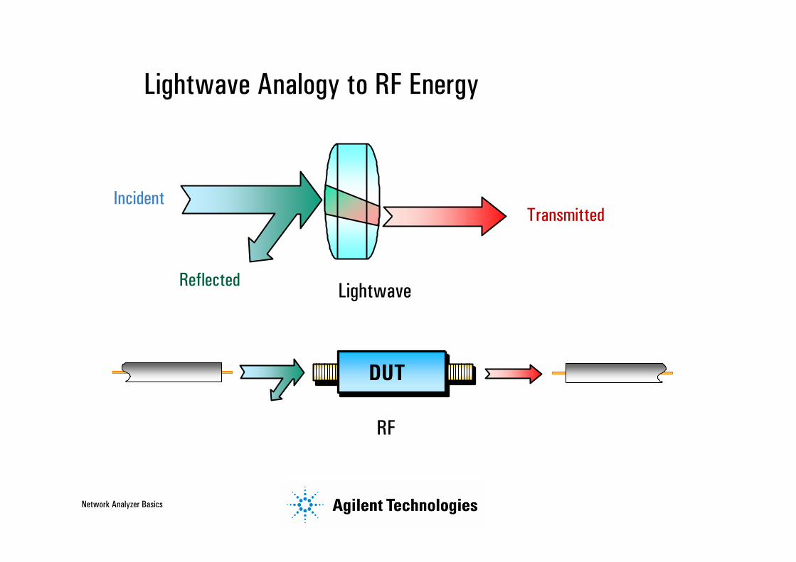
Lightwave Analogy to RF Energy

RF

Incident

Reflected

Transmitted

Lightwave

DUT


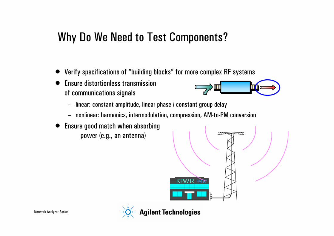
• Verify specifications of “building blocks” for more complex RF systems• Ensure distortionless transmission

of communications signals– linear: constant amplitude, linear phase / constant group delay– nonlinear: harmonics, intermodulation, compression, AM-to-PM conversion

• Ensure good match when absorbing power (e.g., an antenna)

Why Do We Need to Test Components?

KPWR FM 97


The Need for Both Magnitude and Phase

4. Time-domain characterization

Mag

Time

5. Vector-error correction

Error

MeasuredActual

2. Complex impedance needed to design matching circuits

3. Complex values needed for device modeling

1. Complete characterization of linear networks

High-frequency transistor model

Collector

Base

Emitter

S21

S12

S11 S22


Agenda

What measurements do we make?Transmission-line basicsReflection and transmission parametersS-parameter definition

Network analyzer hardwareSignal separation devicesDetection typesDynamic rangeT/R versus S-parameter test sets

Error models and calibrationTypes of measurement errorOne- and two-port modelsError-correction choicesBasic uncertainty calculations

Example measurementsAppendix


Transmission Line Basics

Low frequencieswavelengths >> wire lengthcurrent (I) travels down wires easily for efficient power transmissionmeasured voltage and current not dependent on position along wire

High frequencieswavelength ≈ or << length of transmission mediumneed transmission lines for efficient power transmissionmatching to characteristic impedance (Zo) is very important for low reflection and maximum power transfermeasured envelope voltage dependent on position along line

I+ -


Transmission line Zo• Zo determines relationship between voltage and current waves

• Zo is a function of physical dimensions and εr

• Zo is usually a real impedance (e.g. 50 or 75 ohms)

characteristic impedancefor coaxial airlines (ohms)

10 20 30 40 50 60 70 80 90 100

1.0

0.8

0.7

0.6

0.5

0.9

1.5

1.4

1.3

1.2

1.1

norm

alize

d va

lues

50 ohm standard

attenuation is lowest at 77 ohms

power handling capacity peaks at 30 ohms

Microstrip

h

w

Coplanar

w1

w2

ε r

Waveguide

Twisted-pair

Coaxial

b

a

h


Power Transfer Efficiency

RS

RLFor complex impedances, maximum power transfer occurs when ZL = ZS* (conjugate match)

Maximum power is transferred when RL = RS

RL / RS

0

0.2

0.4

0.6

0.8

1

1.2

0 1 2 3 4 5 6 7 8 9 10

Load

Pow

er

(nor

mal

ized

)

Rs

RL

+jX

-jX


Transmission Line Terminated with Zo

For reflection, a transmission line terminated in Zo behaves like an infinitely long transmission line

Zs = Zo

Zo

Vrefl = 0! (all the incident poweris absorbed in the load)

V inc

Zo = characteristic impedance of transmission line


Transmission Line Terminated with Short, Open

Zs = Zo

Vrefl

V inc

For reflection, a transmission line terminated in a short or open reflects all power back to source

In-phase (0o) for open, out-of-phase (180o) for short


Transmission Line Terminated with 25 Ω

Vrefl

Standing wave pattern does not go to zero as with short or open

Zs = Zo

ZL = 25 Ω

V inc


High-Frequency Device Characterization

Transmitted

Incident

TRANSMISSION

Gain / Loss

S-ParametersS21, S12

GroupDelay

TransmissionCoefficient

Insertion Phase

Reflected

Incident

REFLECTION

SWR

S-ParametersS11, S22 Reflection

Coefficient

Impedance, Admittance

R+jX, G+jB

ReturnLoss

Γ, ρΤ,τ

Incident

Reflected

TransmittedRB

A

A

R=

B

R=


Reflection Parameters

∞ dB

No reflection(ZL = Zo)

ρRL

VSWR

0 1

Full reflection(ZL = open, short)

0 dB

1 ∞

=ZL − ZO

ZL + OZReflection Coefficient =

Vreflected

Vincident= ρ ΦΓ

=ρ ΓReturn loss = -20 log(ρ),

Voltage Standing Wave Ratio

VSWR = Emax

Emin=

1 + ρ1 - ρ

Emax

Emin


Smith Chart Review

∞ →

Smith Chart maps rectilinear impedanceplane onto polar plane

0 +R

+jX

-jX

Rectilinear impedance plane

.

-90 o

0o180 o+-.2

.4.6

.8

1.0

90 o

∞0

Polar plane

Z = ZoL

= 0Γ

Constant X

Constant R

Smith chart

ΓLZ = 0

= ±180 O1

(short) Z = L

= 0 O1Γ(open)


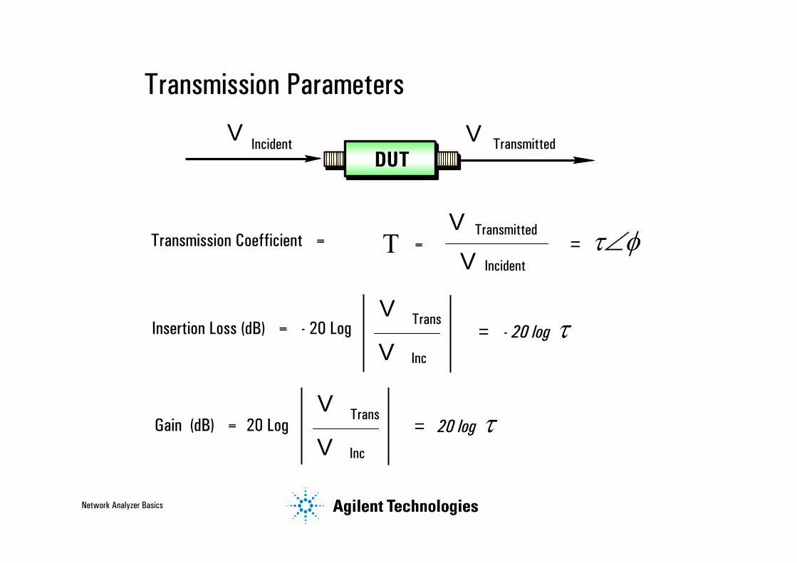
Transmission Parameters

V TransmittedV Incident

Transmission Coefficient = Τ =V Transmitted

V Incident= τ∠φ

DUT

Gain (dB) = 20 Log V Trans

V Inc

= 20 log τ

Insertion Loss (dB) = - 20 Log V Trans

V Inc

= - 20 log τ


Linear Versus Nonlinear Behavior

Linear behavior:input and output frequencies are the same (no additional frequencies created)output frequency only undergoes magnitude and phase change

Frequencyf1

Time

Sin 360o * f * t

Frequency

Aphase shift = to * 360o * f

1f

DUT

Time

A

to

A * Sin 360o * f (t - to)

Input Output

Time

Nonlinear behavior:output frequency may undergo frequency shift (e.g. with mixers)additional frequencies created (harmonics, intermodulation)

Frequencyf1


Criteria for Distortionless TransmissionLinear Networks

Constant amplitude over bandwidth of interest

Mag

nitud

e

Phas

eFrequency

Frequency

Linear phase over bandwidth of interest


Magnitude Variation with Frequency

F(t) = sin wt + 1/3 sin 3wt + 1/5 sin 5wt

Time

Linear Network

Frequency Frequency Frequency

Mag

nitu

de

Time


Phase Variation with Frequency

Frequency

Mag

nitu

de

Linear Network

Frequency

Frequency

Time

0

-180

-360

°

°

°

Time

F(t) = sin wt + 1 /3 sin 3wt + 1 /5 sin 5wt


Deviation from Linear Phase

Use electrical delay to remove linear portion of phase response

Linear electrical length added

+ yields

Frequency

(Electrical delay function)

Frequency

RF filter responseDeviation from linear phase

Phas

e 1

/Div

o

Phas

e 45

/Di

vo

Frequency

Low resolution High resolution


Group Delay

in radians

in radians/sec

in degrees

f in Hertz (ω = 2 π f)

φωφ

Group Delay (t ) g =

−d φd ω =

−1360 o

d φd f*

Frequency

Group delay ripple

Average delay

t o

t g

Phase φ

∆φ

Frequency

∆ωω

group-delay ripple indicates phase distortionaverage delay indicates electrical length of DUTaperture of measurement is very important


Why Measure Group Delay?

Same p-p phase ripple can result in different group delay

Phas

e

Phas

e

Grou

p De

lay

Grou

p De

lay

−d φd ω

−d φd ω

f

f

f

f


Characterizing Unknown Devices

Using parameters (H, Y, Z, S) to characterize devices:gives linear behavioral model of our devicemeasure parameters (e.g. voltage and current) versus frequency under various source and load conditions (e.g. short and open circuits)compute device parameters from measured datapredict circuit performance under any source and load conditions

H-parametersV1 = h11I1 + h12V2

I2 = h21I1 + h22V2

Y-parametersI1 = y11V1 + y12V2

I2 = y21V1 + y22V2

Z-parametersV1 = z11I1 + z12I2

V2 = z21I1 + z22I2

h11 = V1

I1 V2=0

h12 = V1

V2 I1=0

(requires short circuit)

(requires open circuit)


Why Use S-Parameters?

relatively easy to obtain at high frequenciesmeasure voltage traveling waves with a vector network analyzerdon't need shorts/opens which can cause active devices to oscillate or self-destruct

relate to familiar measurements (gain, loss, reflection coefficient ...)can cascade S-parameters of multiple devices to predict system performancecan compute H, Y, or Z parameters from S-parameters if desiredcan easily import and use S-parameter files in our electronic-simulation tools

Incident TransmittedS 21

S 11Reflected S 22

Reflected

Transmitted Incidentb 1

a 1b 2

a 2S 12

DUT

b 1 = S 11 a 1 + S 12 a 2

b 2 = S 21 a 1 + S 22 a 2

Port 1 Port 2


Measuring S-Parameters

S 11 = ReflectedIncident

=b1a 1 a2 = 0

S 21 =Transmitted

Incident=

b2

a 1 a2 = 0

S 22 = ReflectedIncident

=b2a 2 a1 = 0

S 12 =Transmitted

Incident=

b1

a 2 a1 = 0

Incident TransmittedS 21

S 11Reflected

b 1

a 1

b 2

Z 0

Loada2 = 0

DUTForward

IncidentTransmitted S 12

S 22

Reflected

b 2

a 2b

a1 = 0DUTZ 0

Load Reverse

1


Equating S-Parameters with Common Measurement Terms

S11 = forward reflection coefficient (input match)S22 = reverse reflection coefficient (output match)S21 = forward transmission coefficient (gain or loss)S12 = reverse transmission coefficient (isolation)

Remember, S-parameters are inherently complex, linear quantities -- however, we

often express them in a log-magnitude format


Frequency Frequency

TimeTime

Criteria for Distortionless TransmissionNonlinear Networks

• Saturation, crossover, intermodulation, and other nonlinear effects can cause signal distortion

• Effect on system depends on amount and type of distortion and system architecture


Measuring Nonlinear BehaviorMost common measurements:

using a network analyzer and power sweepsgain compressionAM to PM conversion

using a spectrum analyzer + source(s)harmonics, particularly second and thirdintermodulation products resulting

from two or more RF carriersRL 0 dBm ATTEN 10 dB 10 dB / DIV

CENTER 20.00000 MHz SPAN 10.00 kHzRB 30 Hz VB 30 Hz ST 20 sec LPF

8563A SPECTRUM ANALYZER 9 kHz - 26.5 GHz

LPF DUT


What is the Difference Between Network and Spectrum Analyzers?

.Am

plitu

de R

atio

Frequency

Ampl

itude

Frequency


Measures known signal

Measures unknown signals

Network analyzers:measure components, devices, circuits, sub-assembliescontain source and receiverdisplay ratioed amplitude and phase(frequency or power sweeps)offer advanced error correction

Spectrum analyzers:measure signal amplitude characteristicscarrier level, sidebands, harmonics...)can demodulate (& measure) complex signalsare receivers only (single channel)can be used for scalar component test (nophase) with tracking gen. or ext. source(s)


Agenda

What measurements do we make?Network analyzer hardwareError models and calibrationExample measurementsAppendix


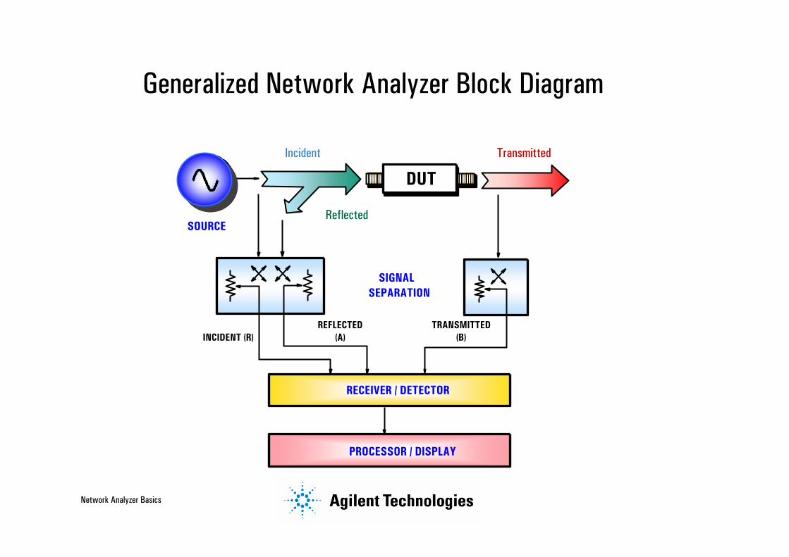
Generalized Network Analyzer Block Diagram

RECEIVER / DETECTOR

PROCESSOR / DISPLAY

REFLECTED(A)

TRANSMITTED(B)INCIDENT (R)

SIGNALSEPARATION

SOURCE

Incident

Reflected

Transmitted

DUT


Source

Supplies stimulus for systemSwept frequency or powerTraditionally NAs used separate sourceMost Agilent analyzers sold today have integrated, synthesized sources


Signal Separation

Test Port

Detectordirectional coupler

splitterbridge

• measure incident signal for reference• separate incident and reflected signals

RECEIVER / DETECTOR

PROCESSOR / DISPLAY

REFLECTED(A)


SIGNALSEPARATION

SOURCE

Incident

Reflected

Transmitted

DUT


Directivity

Directivity is a measure of how well a coupler can separate signals moving in opposite directions

Test port

(undesired leakage signal) (desired reflected signal)

Directional Coupler


Interaction of Directivity with the DUT (Without Error Correction)

Data Max

Add in-phase

Devic

e

Dire

ctivi

ty

Retu

rn L

oss

Frequency

0

30

60

DUT RL = 40 dB

Add out-of-phase (cancellation)

Devic

e

Directivity

Data = Vector Sum

Dire

ctivi

ty Devic

e

Data Min


Detector Types

Tuned Receiver

Scalar broadband(no phase information)

Vector(magnitude and phase)

Diode

DC

ACRF

IF Filter

IF = F LO F RF±RF

LO

ADC / DSP

RECEIVER / DETECTOR

PROCESSOR / DISPLAY

REFLECTED(A)


SIGNALSEPARATION

SOURCE

Incident

Reflected

Transmitted

DUT


Broadband Diode Detection

Easy to make broadbandInexpensive compared to tuned receiverGood for measuring frequency-translating devicesImprove dynamic range by increasing powerMedium sensitivity / dynamic range

10 MHz 26.5 GHz


Narrowband Detection - Tuned Receiver

Best sensitivity / dynamic rangeProvides harmonic / spurious signal rejectionImprove dynamic range by increasing power, decreasing IF bandwidth, or averagingTrade off noise floor and measurement speed

10 MHz 26.5 GHz

ADC / DSP


Comparison of Receiver Techniques

< -100 dBm Sensitivity

0 dB

-50 dB

-100 dB

0 dB

-50 dB

-100 dB

-60 dBm Sensitivity

Broadband (diode) detection

Narrowband (tuned-receiver) detection

higher noise floorfalse responses

high dynamic rangeharmonic immunity

Dynamic range = maximum receiver power - receiver noise floor


Dynamic Range and Accuracy

Dynamic range is very important for

measurement accuracy!

Error Due to Interfering Signal

0.001

0.01

0.1

1

10

100

0 -5 -10 -15 -20 -25 -30 -35 -40 -45 -50 -55 -60 -65 -70

Interfering signal (dB)

Erro

r (dB

, deg

) phase error

magn error

+

-


T/R Versus S-Parameter Test Sets

RF always comes out port 1port 2 is always receiverresponse, one-port cal available

RF comes out port 1 or port 2forward and reverse measurementstwo-port calibration possible

Transmission/Reflection Test Set

Port 1 Port 2

Source

B

R

A

DUTFwd

Port 1 Port 2

Transfer switch

Source

B

R

A

S-Parameter Test Set

DUTFwd Rev


RECEIVER / DETECTOR

PROCESSOR / DISPLAY

REFLECTED(A)


SIGNALSEPARATION

SOURCE

Incident

Reflected

Transmitted

DUT

Processor / Display

CH1 S21 log MAG 10 dB/ REF 0 dB

CH1 START 775.000 000 MHz STOP 925.000 000 MHz

CorHld

PRmCH2 S12 log MAG REF 0 dB10 dB/


Duplexer Test - Tx-Ant and Ant-Rx

CorHld

PRm

1

1

1_ -1.9248 dB

839.470 000 MHz

PASS

2

1

1_ -1.2468 dB

880.435 000 MHz

PASS

markerslimit linespass/fail indicatorslinear/log formatsgrid/polar/Smith charts

ACTIVE CHANNEL

RESPONSE

STIMULUS

ENTRY

INSTRUMENT STATE R CHANNEL

R LT S

HP-IB STATUS

NETWORK ANYZER50 MH-20GHz

PORT 2PORT 1

CH1 S21 log M AG 10 dB/ REF 0 dB

CH1 START 775.000 000 M Hz S TO P 925.000 000 M Hz

CorH ld

PRmCH2 S12 log M AG REF 0 dB10 dB/

CH2 START 775.000 000 M Hz S TO P 925.000 000 M Hz

D uplexer Test - Tx-Ant and A nt-Rx

CorH ld

PRm

1

1

1_ -1.9248 dB

839.470 000 M Hz

PA SS

2

1

1_ -1.2468 dB

880.435 000 M Hz

PA SS


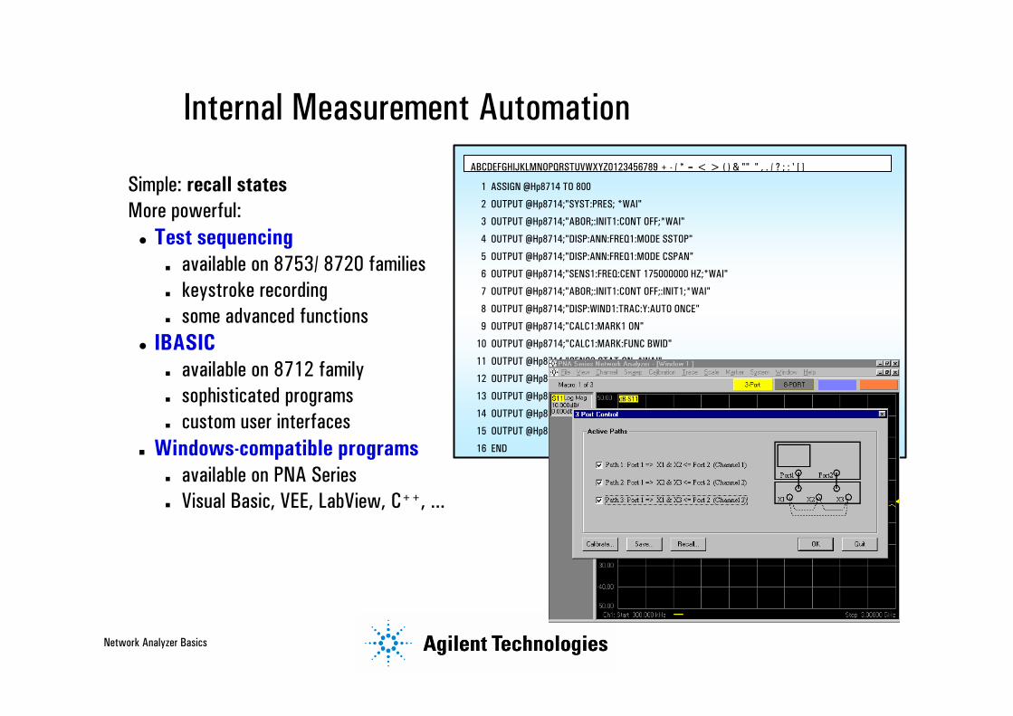
Internal Measurement Automation

Simple: recall statesMore powerful:

Test sequencingavailable on 8753/ 8720 familieskeystroke recordingsome advanced functions

IBASICavailable on 8712 familysophisticated programscustom user interfaces

Windows-compatible programsavailable on PNA SeriesVisual Basic, VEE, LabView, C++, ...

ABCDEFGHIJKLMNOPQRSTUVWXYZ0123456789 + - / * = < > ( ) & "" " , . / ? ; : ' [ ]

1 ASSIGN @Hp8714 TO 800

2 OUTPUT @Hp8714;"SYST:PRES; *WAI"

3 OUTPUT @Hp8714;"ABOR;:INIT1:CONT OFF;*WAI"

4 OUTPUT @Hp8714;"DISP:ANN:FREQ1:MODE SSTOP"

5 OUTPUT @Hp8714;"DISP:ANN:FREQ1:MODE CSPAN"

6 OUTPUT @Hp8714;"SENS1:FREQ:CENT 175000000 HZ;*WAI"

7 OUTPUT @Hp8714;"ABOR;:INIT1:CONT OFF;:INIT1;*WAI"

8 OUTPUT @Hp8714;"DISP:WIND1:TRAC:Y:AUTO ONCE"

9 OUTPUT @Hp8714;"CALC1:MARK1 ON"

10 OUTPUT @Hp8714;"CALC1:MARK:FUNC BWID"

11 OUTPUT @Hp8714;"SENS2:STAT ON; *WAI"

12 OUTPUT @Hp8714;"SENS2:FUNC 'XFR:POW:RAT 1,0';DET NBAN; *WAI"

13 OUTPUT @Hp8714;"ABOR;:INIT1:CONT OFF;:INIT1;*WAI"

14 OUTPUT @Hp8714;"DISP:WIND2:TRAC:Y:AUTO ONCE"

15 OUTPUT @Hp8714;"ABOR;:INIT1:CONT ON;*WAI"

16 END


Agilent’s Series of HF Vector AnalyzersMicrowave

RF

8510C series110 GHz in coaxhighest accuracymodular, flexiblepulse systems

8720/22 ET/ES series13.5, 20, 40 GHzeconomicalfast, small, integratedtest mixers, high-power amps

8753ET/ES series3, 6 GHzflexible hardwarerich feature set offset and harmonic RF sweeps

PNA Series3, 6, 9 GHzhighest RF performanceadvanced connectivityinternal automation, SCPI or COM/DCOM


Agilent’s LF/RF Vector Analyzers

E5100A/B180, 300 MHzeconomicalfast, smalltarget markets: crystals, resonators, filtersequivalent-circuit modelsevaporation-monitor-function option

4395A/4396B500 MHz (4395A), 1.8 GHz (4396B)impedance-measuring optionfast, FFT-based spectrum analysistime-gated spectrum-analyzer optionIBASICstandard test fixtures

LF

Combination NA / SA

8712/14 ET/ES series1.3, 3 GHzlow costnarrowband and broadband detectionIBASIC / LAN

RF


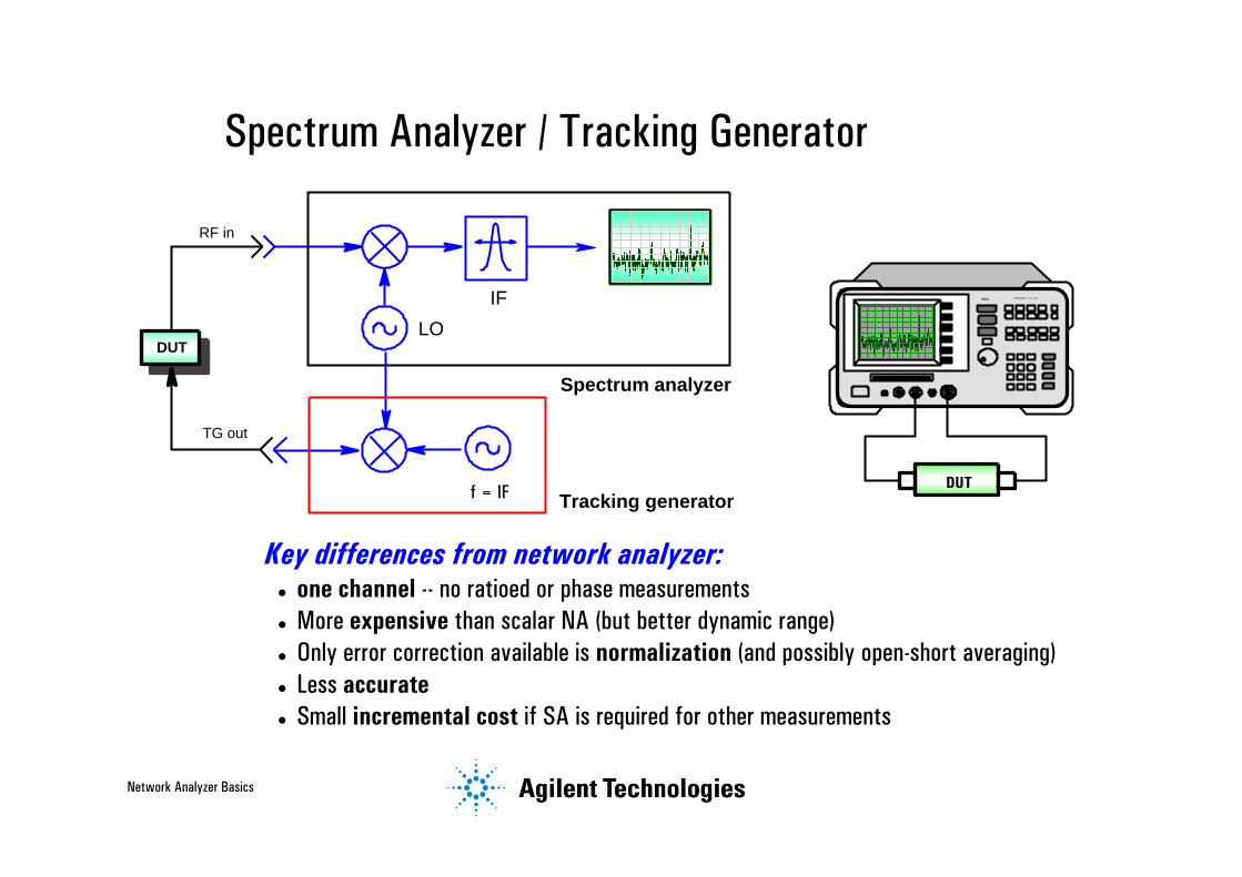
Spectrum Analyzer / Tracking Generator

Tracking generator

RF in

TG out

f = IF

Spectrum analyzer

IFLO

DUT

Key differences from network analyzer:one channel -- no ratioed or phase measurementsMore expensive than scalar NA (but better dynamic range)Only error correction available is normalization (and possibly open-short averaging)Less accurateSmall incremental cost if SA is required for other measurements


DUT


Agenda

Why do we even need error-correction and calibration?It is impossible to make perfect hardwareIt would be extremely expensive to make hardware good enough to eliminate the need for error correction



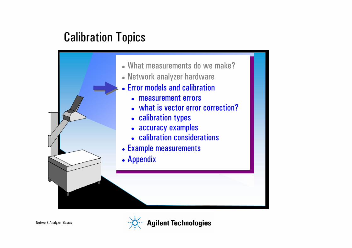
Calibration Topics

What measurements do we make?Network analyzer hardwareError models and calibration

measurement errorswhat is vector error correction?calibration typesaccuracy examplescalibration considerations

Example measurementsAppendix


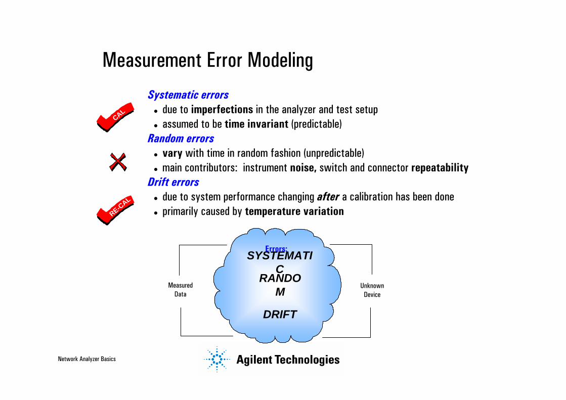
Systematic errorsdue to imperfections in the analyzer and test setupassumed to be time invariant (predictable)

Random errorsvary with time in random fashion (unpredictable)main contributors: instrument noise, switch and connector repeatability

Drift errorsdue to system performance changing after a calibration has been doneprimarily caused by temperature variation

Measurement Error Modeling

Measured Data

Unknown Device

SYSTEMATIC

RANDOM

DRIFT

Errors:

CAL

RE-CAL


Systematic Measurement Errors

A B

SourceMismatch

LoadMismatch

CrosstalkDirectivity

DUT

Frequency responsereflection tracking (A/R)transmission tracking (B/R)

R

Six forward and six reverse error terms yields 12 error terms for two-port devices


Types of Error Correction

response (normalization)simple to performonly corrects for tracking errorsstores reference trace in memory,then does data divided by memory

vectorrequires more standardsrequires an analyzer that can measure phaseaccounts for all major sources of systematic error

S11 m

S11 a

SHORT

OPEN

LOAD

thru

thru


What is Vector-Error Correction?

Process of characterizing systematic error termsmeasure known standardsremove effects from subsequent measurements

1-port calibration (reflection measurements)only 3 systematic error terms measureddirectivity, source match, and reflection tracking

Full 2-port calibration (reflection and transmission measurements)12 systematic error terms measuredusually requires 12 measurements on four known standards (SOLT)

Standards defined in cal kit definition filenetwork analyzer contains standard cal kit definitionsCAL KIT DEFINITION MUST MATCH ACTUAL CAL KIT USED!User-built standards must be characterized and entered into user cal-kit


Reflection: One-Port Model

ED = Directivity

ERT = Reflection tracking

ES = Source Match

S11M = Measured

S11A = Actual

To solve for error terms, we measure 3 standards to generate

3 equations and 3 unknowns

S11M

S11AES

ERT

ED

1RF in

Error Adapter

S11M

S11A

RF in Ideal

Assumes good termination at port two if testing two-port devicesIf using port 2 of NA and DUT reverse isolation is low (e.g., filter passband):

assumption of good termination is not valid two-port error correction yields better results

S11M = ED + ERT1 - ES S11A

S11A


Before and After One-Port Calibration

data before 1-port calibration

data after 1-port calibration

0

20

40

60

6000 12000

2.0

Retu

rn L

oss

(dB)

VSW

R

1.1

1.01

1.001

MHz


Two-Port Error Correction

Each actual S-parameter is a function of all four measured S-parametersAnalyzer must make forward and reverse sweep to update any one S-parameterLuckily, you don't need to know these equations to use network analyzers!!!

Port 1 Port 2E

S11

S21

S12

S22

ESED

ERT

ETT

EL

a1

b1

A

A

A

A

X

a2

b2

Forward model

= fwd directivity= fwd source match= fwd reflection tracking

= fwd load match= fwd transmission tracking= fwd isolation

ES

ED

ERT

ETT

EL

EX

= rev reflection tracking= rev transmission tracking

= rev directivity= rev source match

= rev load match

= rev isolationES'

ED'

ERT'

ETT'

EL'

EX'

Port 1 Port 2

S11

S

S12

S22 ES'ED'

ERT'

ETT'

EL'a1

b1A

A

A

EX'

21A

a2

b2

Reverse model

S a

S m ED

ERT

S m ED

ERT

ES E LS m E X

ETT

S m E X

ETT

S m ED'

ERT

ES

S m ED

ERT

ES E L E LS m E X

ETT

S m E X

ETT

11

11 1 22 21 12

1 11 1 22 21 12

=

−

+

−

−

− −

+

−

+

−

−

− −

( )(

'

'

' ) ( )(

'

'

)

( )(

'

'

' ) ' ( )(

'

'

)

S a

S m E X

ETT

S m ED

ERT

ES E L

S m ED

ERT

ES

S m E D

ERT

ES E L

21

21 22

1 11 1 22

=

−

1 +

−

−

+

−

+

−

−

( )(

'

'

( ' ))

( )(

'

'

' ) ' ( )(

'

'

)E LS m E X

ETT

S m E X

ETT

21 12− −

'S E S E− −

(

'

)( ( ' ))

( )(

'

'

' ) ' ( )(

'

'

)

m X

ETT

m D

ERT

ES E L

S m ED

ERT

ES

S m E D

ERT

ES E L E LS m E X

ETT

S m E X

ETT

S a

12 1 11

1 11 1 22 21 12

12

+ −

+

−

+

−

−

− −

=

(

'

'

)(

(

S m ED

ERT

S m ED

ERT

S a

22

1 11

22

−

) ' ( )(

'

'

)

S m ED

ERT

ES E L

S m E X

ETT

S m E X

ETT

11 21 12−

−

− −

+

−

=

ES

S m E D

ERT

ES E L E LS m E X

ETT

S m E X

ETT

)(

'

'

' ) ' ( )(

'

'

)1 22 21 12+

−

−

− −

1 +


Crosstalk: Signal Leakage Between Test Ports During Transmission

Can be a problem with:high-isolation devices (e.g., switch in open position)high-dynamic range devices (some filter stopbands)

Isolation calibrationadds noise to error model (measuring near noise floor of system)only perform if really needed (use averaging if necessary)if crosstalk is independent of DUT match, use two terminationsif dependent on DUT match, use DUT with termination on output

DUT

DUT LOADDUTLOAD


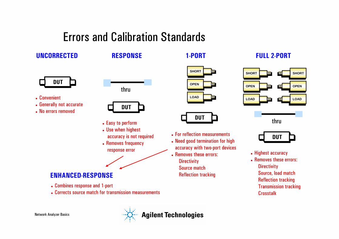
Errors and Calibration Standards

ConvenientGenerally not accurateNo errors removed

Easy to performUse when highestaccuracy is not required

Removes frequencyresponse error

For reflection measurementsNeed good termination for high accuracy with two-port devicesRemoves these errors:

DirectivitySource matchReflection tracking

Highest accuracyRemoves these errors:

DirectivitySource, load matchReflection trackingTransmission trackingCrosstalk

UNCORRECTED RESPONSE 1-PORT FULL 2-PORT

DUT

DUT

DUT

DUT

thru

thru

ENHANCED-RESPONSECombines response and 1-portCorrects source match for transmission measurements

SHORT

OPEN

LOAD

SHORT

OPEN

LOAD

SHORT

OPEN

LOAD


Transmission Tracking

Crosstalk

Source match

Load match

S-parameter(two-port)

T/R(response, isolation)

TransmissionTest Set (cal type)

*( )

Calibration Summary

Reflection tracking

Directivity

Source match

Load match

S-parameter(two-port)

T/R(one-port)

ReflectionTest Set (cal type)

error cannot be corrected

* enhanced response cal corrects for source match during transmission measurements

error can be corrected

SHORT

OPEN

LOAD


Reflection Example Using a One-Port Cal

DUT16 dB RL (.158)1 dB loss (.891)

Load match:18 dB (.126)

.158

(.891)(.126)(.891) = .100

Directivity:40 dB (.010)

Measurement uncertainty:-20 * log (.158 + .100 + .010)= 11.4 dB (-4.6dB)

-20 * log (.158 - .100 - .010)= 26.4 dB (+10.4 dB)

Remember: convert all dB values to linear for uncertainty calculations!

ρ or loss(linear) = 10( )-dB

20


Using a One-Port Cal + Attenuator

Low-loss bi-directional devicesgenerally require two-port calibration

for low measurement uncertainty

Load match:18 dB (.126)

DUT16 dB RL (.158)1 dB loss (.891)

10 dB attenuator (.316) SWR = 1.05 (.024)

.158

(.891)(.316)(.126)(.316)(.891) = .010

(.891)(.024)(.891) = .019

Directivity:40 dB (.010)

Worst-case error = .010 + .010 + .019 = .039

Measurement uncertainty:-20 * log (.158 + .039)= 14.1 dB (-1.9 dB)

-20 * log (.158 - .039)= 18.5 dB (+2.5 dB)


Transmission Example Using Response Cal

RL = 14 dB (.200)

RL = 18 dB (.126)

Thru calibration (normalization) builds error into measurement due to source and load match interaction

Calibration Uncertainty= (1± ρS ρL)

= (1 ± (.200)(.126)= ± 0.22 dB


Filter Measurement with Response Cal

Source match = 14 dB (.200)

1

(.126)(.158) = .020

(.158)(.200) = .032

(.126)(.891)(.200)(.891) = .020

Measurement uncertainty= 1 ± (.020+.020+.032)= 1 ± .072= + 0.60 dB

- 0.65 dB

DUT1 dB loss (.891)16 dB RL (.158)

Total measurement uncertainty:+0.60 + 0.22 = + 0.82 dB-0.65 - 0.22 = - 0.87 dB

Load match = 18 dB (.126)


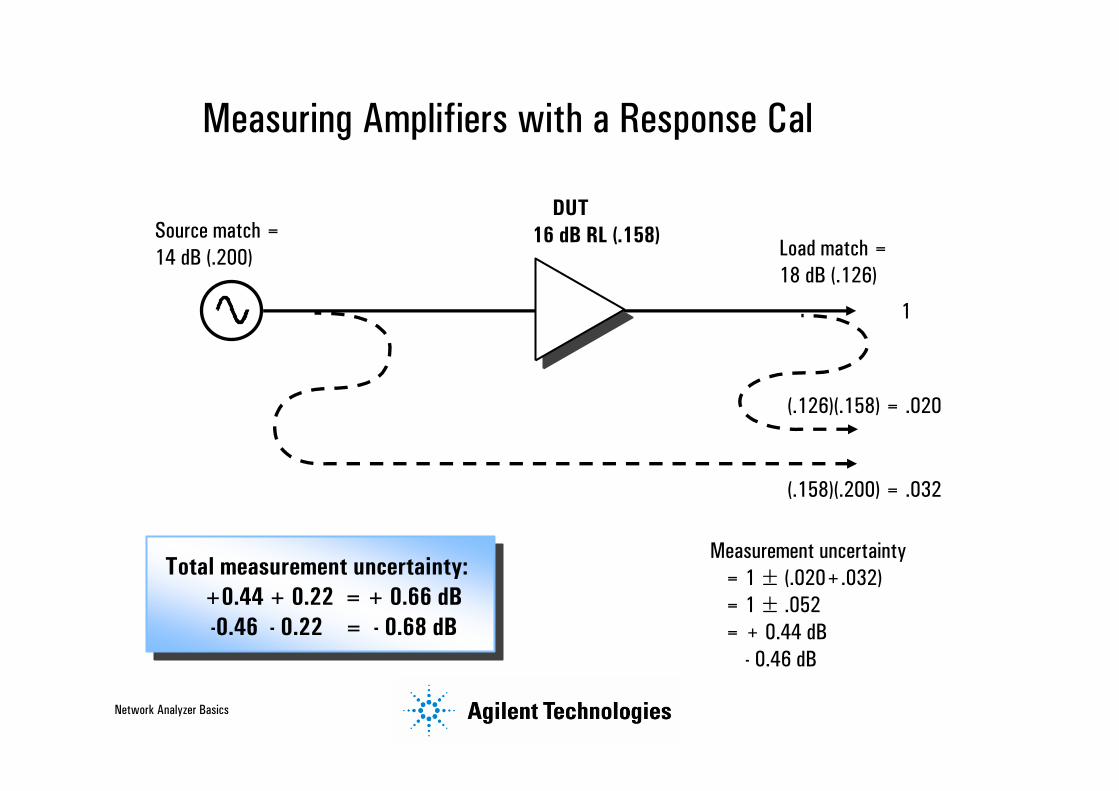
Measuring Amplifiers with a Response Cal

Total measurement uncertainty:+0.44 + 0.22 = + 0.66 dB-0.46 - 0.22 = - 0.68 dB

Measurement uncertainty= 1 ± (.020+.032)= 1 ± .052= + 0.44 dB

- 0.46 dB

1

(.126)(.158) = .020

DUT16 dB RL (.158)

(.158)(.200) = .032

Source match = 14 dB (.200) Load match =

18 dB (.126)


Filter Measurements using the Enhanced Response

Calibration

Measurement uncertainty= 1 ± (.020+.0018+.0028)= 1 ± .0246= + 0.211 dB

- 0.216 dB

Total measurement uncertainty:0.22 + .02 = ± 0.24 dB

Calibration Uncertainty= Effective source match = 35 dB!


1

(.126)(.158) = .020

(.126)(.891)(.0178)(.891) = .0018

DUT1 dB loss (.891)16 dB RL (.158) Load match =

18 dB (.126)

(.158)(.0178) = .0028

(1± ρS ρL)= (1 ± (.0178)(.126)= ± .02 dB


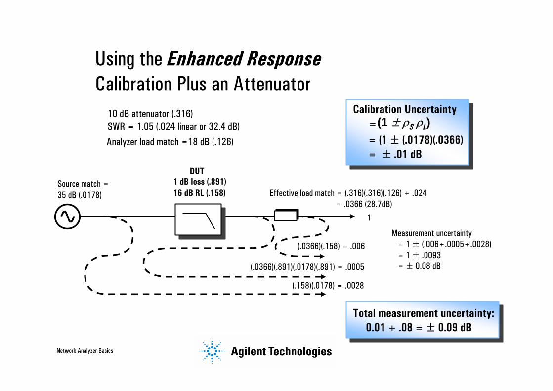
Using the Enhanced Response Calibration Plus an Attenuator

Measurement uncertainty= 1 ± (.006+.0005+.0028)= 1 ± .0093= ± 0.08 dB

Total measurement uncertainty:0.01 + .08 = ± 0.09 dB


1

(.0366)(.158) = .006

(.0366)(.891)(.0178)(.891) = .0005

DUT1 dB loss (.891)16 dB RL (.158) Effective load match = (.316)(.316)(.126) + .024

= .0366 (28.7dB)

(.158)(.0178) = .0028

10 dB attenuator (.316) SWR = 1.05 (.024 linear or 32.4 dB)

Analyzer load match =18 dB (.126)

Calibration Uncertainty= = (1 ± (.0178)(.0366)= ± .01 dB

(1± ρS ρL)


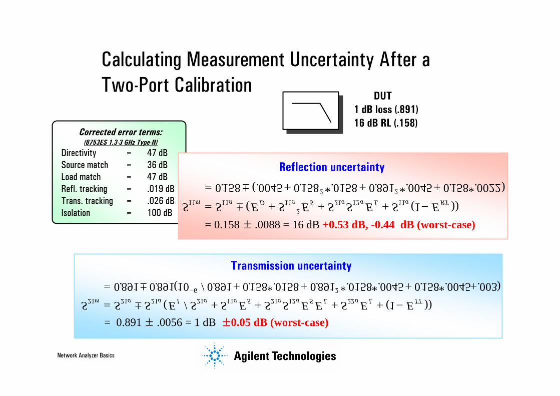
Calculating Measurement Uncertainty After a Two-Port Calibration

Corrected error terms:(8753ES 1.3-3 GHz Type-N)

Directivity = 47 dBSource match = 36 dBLoad match = 47 dBRefl. tracking = .019 dB Trans. tracking = .026 dBIsolation = 100 dB

DUT1 dB loss (.891)16 dB RL (.158)

Transmission uncertainty

= 0.891 ± .0056 = 1 dB ±0.05 dB (worst-case)

Reflection uncertainty

= 0.158 ± .0088 = 16 dB +0.53 dB, -0.44 dB (worst-case)

S S E S E S S E S Em a D a S a a L a RT11 11 112

21 12 11

2 2

1

0158 0045 0158 0158 0 891 0045 0158 0022

= ± + + + −

= ± + + +

( ( ))

. (. . *. . *. . *. )

S S S E S S E S S E E S E Em a a I a a S a a S L a L TT21 21 21 21 11 21 12 22

6 2

1

0 891 0 891 10 0 891 0158 0158 0 891 0158 0045 0158 0045 003

= ± + + + + −

= ± + + + +

−

( / ( ))

. . ( / . . *. . *. *. . *. . )


Comparison of Measurement Examples

Calibration type Calibration uncertainty Measurement uncertainty Total uncertaintyResponse ±0.22 dB 0.60/ -0.65 dB 0.82/ -0.87Enhanced response ±0.02 dB ±0.22 dB ±0.24Enh. response + attenuator ±0.01 dB ±0.08 dB ±0.09Two port ----- ±0.05

Calibration type Measurement uncertaintyOne-port -4.6/ 10.4 dBOne-port + attenuator -1.9/ 2.5 dBTwo-port -0.44/ 0.53 dB

Reflection

Transmission


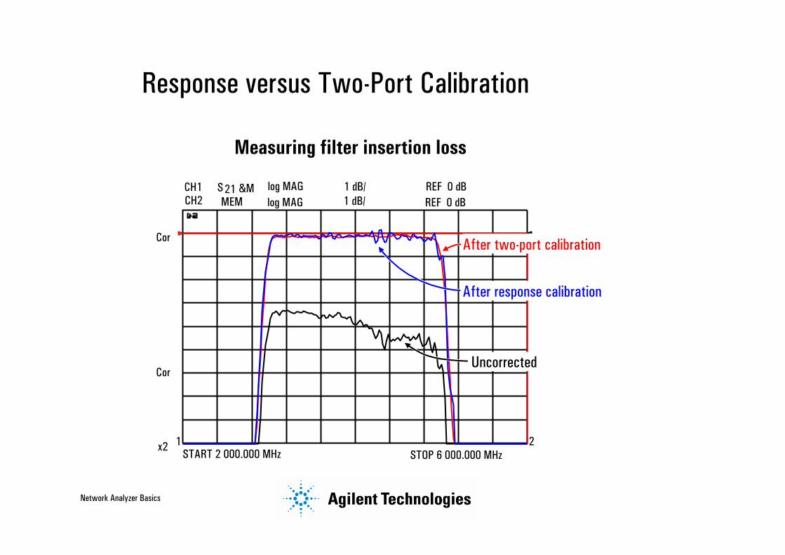
Response versus Two-Port Calibration

CH1 S 21 &M log MAG 1 dB/ REF 0 dB

Cor

CH2 MEM log MAG REF 0 dB1 dB/

CorUncorrected

After two-port calibration

START 2 000.000 MHz STOP 6 000.000 MHzx2 1 2

After response calibration

Measuring filter insertion loss


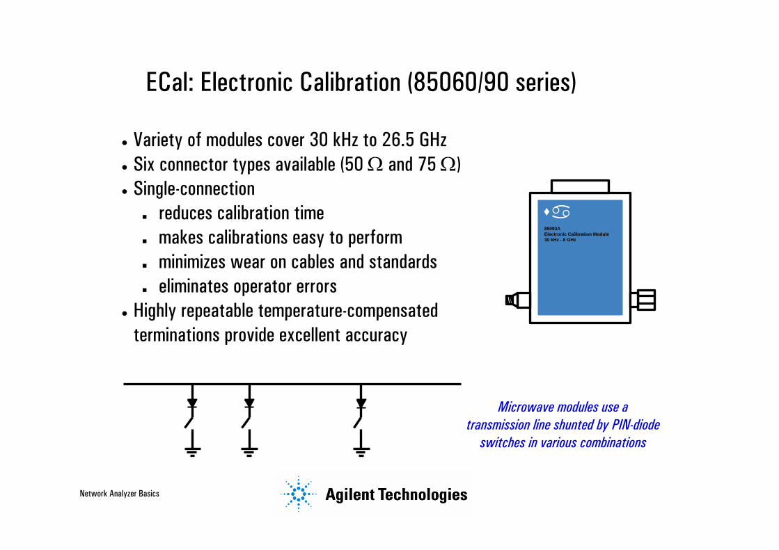
• Variety of modules cover 30 kHz to 26.5 GHz• Six connector types available (50 Ω and 75 Ω)• Single-connection

reduces calibration timemakes calibrations easy to performminimizes wear on cables and standardseliminates operator errors

• Highly repeatable temperature-compensated terminations provide excellent accuracy

ECal: Electronic Calibration (85060/90 series)

85093A Electronic Calibration Module30 kHz - 6 GHz

Microwave modules use a transmission line shunted by PIN-diode

switches in various combinations


Adapter Considerations

TerminationAdapter DUT

Coupler directivity = 40 dB

leakage signal

desired signalreflection from adapter

APC-7 calibration done here

DUT has SMA (f) connectors

= measured ρ +adapter

ρDUT

ρDirectivity +

Worst-caseSystem Directivity

28 dB

17 dB

14 dB

APC-7 to SMA (m)SWR:1.06

APC-7 to N (f) + N (m) to SMA (m)SWR:1.05 SWR:1.25

APC-7 to N (m) + N (f) to SMA (f) + SMA (m) to (m)SWR:1.05 SWR:1.25 SWR:1.15

Adapting from APC-7 to SMA (m)


Calibrating Non-Insertable Devices

When doing a through cal, normally test ports mate directlycables can be connected directly without an adapterresult is a zero-length through

What is an insertable device?has same type of connector, but different sex on each porthas same type of sexless connector on each port (e.g. APC-7)

What is a non-insertable device?one that cannot be inserted in place of a zero-length throughhas same connectors on each port (type and sex)has different type of connector on each port

(e.g., waveguide on one port, coaxial on the other)What calibration choices do I have for non-insertable devices?

use an uncharacterized through adapteruse a characterized through adapter (modify cal-kit definition)swap equal adaptersadapter removal

DUT


Swap Equal Adapters Method

DUTPort 1 Port 2

1. Transmission cal using adapter A.

2. Reflection cal using adapter B.

3. Measure DUT using adapter B.

Port 1 Port 2Adapter A

Adapter B

Port 1 Port 2

Adapter B

Port 1 Port 2DUT

Accuracy depends on how well the adapters are matched - loss, electrical length, match

and impedance should all be equal


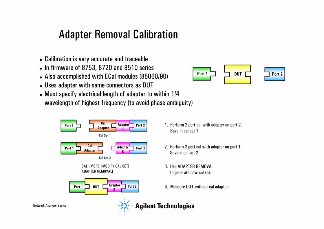
Adapter Removal Calibration

Calibration is very accurate and traceableIn firmware of 8753, 8720 and 8510 seriesAlso accomplished with ECal modules (85060/90)Uses adapter with same connectors as DUTMust specify electrical length of adapter to within 1/4 wavelength of highest frequency (to avoid phase ambiguity)

DUTPort 1 Port 2

1. Perform 2-port cal with adapter on port 2.Save in cal set 1.

2. Perform 2-port cal with adapter on port 1.Save in cal set 2.

4. Measure DUT without cal adapter.

3. Use ADAPTER REMOVALto generate new cal set.

[CAL] [MORE] [MODIFY CAL SET][ADAPTER REMOVAL]

Cal Set 1

Port 1 Port 2Adapter B

Cal Adapter

Cal Adapter

Cal Set 2

Port 1 Port 2Adapter B

Port 2Adapter B

DUTPort 1


Thru-Reflect-Line (TRL) Calibration

We know about Short-Open-Load-Thru (SOLT) calibration...What is TRL?

A two-port calibration techniqueGood for noncoaxial environments (waveguide, fixtures, wafer probing)Uses the same 12-term error model as the more common SOLT calUses practical calibration standards thatare easily fabricated and characterized Two variations: TRL (requires 4 receivers) and TRL* (only three receivers needed)Other variations: Line-Reflect-Match (LRM),

Thru-Reflect-Match (TRM), plus many others

TRL was developed for non-coaxial microwave measurements


Agenda



Frequency Sweep - Filter TestCH1 S11 log MAG 5 dB/ REF 0 dB

CENTER 200.000 MHz SPAN 50.000 MHz

Return loss

log MAG 10 dB/ REF 0 dBCH1 S21

START .300 000 MHz STOP 400.000 000 MHz

Cor

69.1 dB Stopband rejection

Insertion loss

SCH1 21 log MAG 1 dB/ REF 0 dB

Cor

Cor

START 2 000.000 MHz STOP 6 000.000 MHzx2 1 2

m1: 4.000 000 GHz -0.16 dBm2-ref: 2.145 234 GHz 0.00 dB

1

ref 2


Segment 3: 29 ms (108 points, -10 dBm, 6000 Hz)

Optimize Filter Measurements with Swept-List Mode


START 525.000 000 MHz

PRm

PASS

STOP 1 275.000 000 MHz

Segment 1: 87 ms (25 points, +10 dBm, 300 Hz)

Segments 2,4: 52 ms (15 points, +10 dBm, 300 Hz)

Segment 5: 129 ms (38 points, +10 dBm, 300 Hz)

Linear sweep: 676 ms(201 pts, 300 Hz, -10 dBm)

Swept-list sweep: 349 ms(201 pts, variable BW's & power)


Power Sweeps - Compression

Saturated output powerOu

tput

Pow

er (d

Bm)

Input Power (dBm)

Compression region

Linear region(slope = small-signal gain)


CH1 S21 1og MAG 1 dB/ REF 32 dB 30.991 dB12.3 dBm

Power Sweep - Gain Compression

0

START -10 dBm CW 902.7 MHz STOP 15 dBm

1

1 dB compression:

input power resulting in 1 dB drop in gain


AM to PM Conversion

AM - PM Conversion =

Mag(Pmout)Mag(Amin)

(deg/dB)

DUT

Amplitude

Time

AM (dB)

PM (deg)

Mag(AMout)

Mag(Pmout)

Output Response

Amplitude

Time

AM (dB)

PM (deg)

Mag(Amin)

Test Stimulus

Power sweep

I

Q

AM to PM conversion can cause bit errors

Measure of phase deviation caused by amplitude variations

AM can be undesired:supply ripple, fading, thermalAM can be desired:

modulation (e.g. QAM)


Measuring AM to PM Conversion

Use transmission setupwith a power sweep

Display phase of S21AM - PM = 0.86 deg/dB

Stop 0.00 dBm

Ref 21.50 dB

Stop 0.00 dBm

1:Transmission Log Mag 1.0 dB/

Start -10.00 dBm CW 900.000 MHzStart -10.00 dBm CW 900.000 MHz

2:Transmission /M Phase 5.0 deg/ Ref -115.7 deg

1

2

1

1

2

Ch1:Mkr1 -4.50 dBm 20.48 dB

Ch2:Mkr2 1.00 dB 0.86 deg


Agenda


Advanced Topicstime domain frequency-translating deviceshigh-power amplifiersextended dynamic rangemultiport devicesin-fixture measurementscrystal resonatorsbalanced measurements

Inside the network analyzerChallenge quiz!


Time-Domain Reflectometry (TDR)

What is TDR?time-domain reflectometryanalyze impedance versus timedistinguish between inductive and capacitive transitions

With gating:analyze transitionsanalyzer standards

Zotime

impe

danc

e

non-Zo transmission line

inductive transition

capacitive transition


start with broadband frequency sweep (often requires microwave VNA)use inverse-Fourier transform to compute time-domainresolution inversely proportionate to frequency span

CH1 S 22 Re 50 mU/ REF 0 U

CH1 START 0 s STOP 1.5 ns

Cor 20 GHz

6 GHz

Time Domain Frequency Domain

t

f

1/s*F(s)F(t)*dt∫0

t

Integrate

ft

f

TDRF -1

TDR Basics Using a Network Analyzer

F -1


Time-Domain GatingTDR and gating can remove undesired reflections (a form of error correction)Only useful for broadband devices (a load or thru for example)Define gate to only include DUTUse two-port calibration

CH1 MEM Re 20 mU/ REF 0 U

CH1 START 0 s STOP 1.5 ns

CorPRm

RISE TIME29.994 ps8.992 mm 1

2

3

1: 48.729 mU 638 ps

2: 24.961 mU 668 ps

3: -10.891 mU 721 ps

Thru in time domain

CH1 S11 &M log MAG 5 dB/ REF 0 dB

START .050 000 000 GHz STOP 20.050 000 000 GHz

Gate

Cor

PRm

1

2

2: -15.78 dB 6.000 GHz

1: -45.113 dB 0.947 GHz

Thru in frequency domain, with and without gating


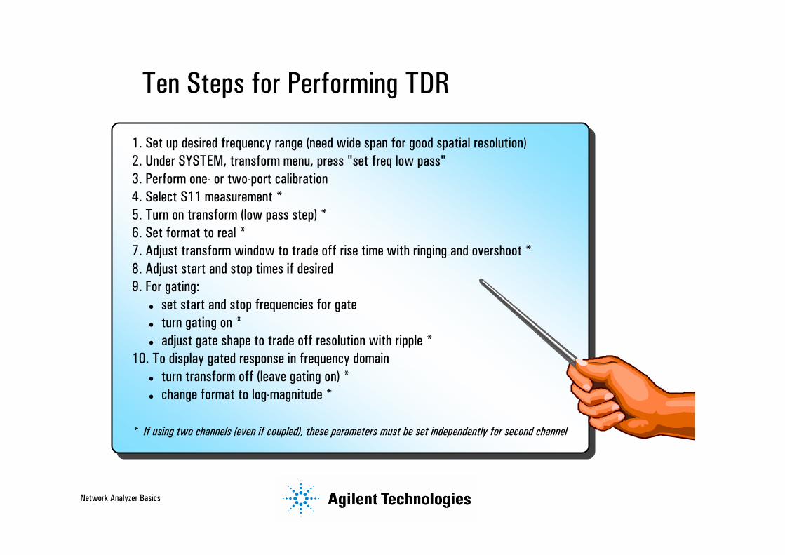
Ten Steps for Performing TDR

1. Set up desired frequency range (need wide span for good spatial resolution)2. Under SYSTEM, transform menu, press "set freq low pass"3. Perform one- or two-port calibration4. Select S11 measurement *5. Turn on transform (low pass step) *6. Set format to real *7. Adjust transform window to trade off rise time with ringing and overshoot *8. Adjust start and stop times if desired9. For gating:

set start and stop frequencies for gateturn gating on *adjust gate shape to trade off resolution with ripple *

10. To display gated response in frequency domainturn transform off (leave gating on) *change format to log-magnitude *

* If using two channels (even if coupled), these parameters must be set independently for second channel


Time-Domain Transmission


START -1 us STOP 6 us

Cor RF Leakage

SurfaceWave

TripleTravel

RF Output

RF Input

Triple Travel

Main WaveLeakage


Cor

Gate on

Gate off


Time-Domain Filter Tuning

• Deterministic method used for tuning cavity-resonator filters

• Traditional frequency-domain tuning is very difficult:

lots of training neededmay take 20 to 90 minutes to tune a single filter

• Need VNA with fast sweep speeds and fast time-domain processing


Filter Reflection in Time Domain

• Set analyzer’s center frequency = center frequency of the filter

• Measure S11 or S22 in the time domain• Nulls in the time-domain response correspond

to individual resonators in filter


Tuning Resonator #3

• Easier to identify mistuned resonator in time-domain: null #3 is missing

• Hard to tell which resonator is mistuned from frequency-domain response

• Adjust resonators by minimizing null• Adjust coupling apertures using

the peaks in-between the dips


Frequency-Translating DevicesMedium-dynamic range measurements (35 dB)

High-dynamic range measurements (100 dB)

Filter

Reference mixer

Ref out

Ref in

Attenuator

Attenuator

Power splitter

ESG-D4000A

DUT

Attenuator

8753ES

Filter

AttenuatorAttenuator

Ref In

Start: 900 MHzStop: 650 MHz

Start: 100 MHzStop: 350 MHz

Fixed LO: 1 GHzLO power: 13 dBm

FREQ OFFS

ON off

LOMENU

DOWNCONVERTER

UP

CONVERTER

RF > LO

RF < LO

VIEW MEASURE

RETURN

8753ES

1 2

CH1 CONV MEAS log MAG 10 dB/ REF 10 dB

START 640.000 000 MHz STOP 660.000 000 MHz


High-Power Amplifiers

Source

B

R

A

+43 dBm max input (20 watts!)

Preamp

AUT

8720ES Option 085

DUT

Ref In

AUT

Preamp

8753ES

85118A High-Power Amplifier Test System


High-Dynamic Range Measurements

-150-140-130-120-110-100

-90-80-70-60-50-40-30-20-10

0

800 980MHz

Take advantage of extended dynamic range with direct-receiver access


Multiport Device Test

log MAG 10 dB/ REF 0 dB 1_ -1.9248 dBCH1 S21


Cor

Hld

PRm

CH2 S12 log MAG REF 0 dB10 dB/


Cor

Hld

PRm

1

1

839.470 000 MHz

PASS

2

1

1_ -1.2468 dB

880.435 000 MHz

PASS

Duplexer Test - Tx-Ant and Ant-Rx

Multiport analyzers and test sets:improve throughput by reducing the number of connections to DUTs with more than two portsallow simultaneous viewing of two paths(good for tuning duplexers)include mechanical or solid-state switches, 50 or 75 ohmsdegrade raw performance so calibration is a must (use two-port cals whenever possible)Agilent offers a variety of standard and custom multiport analyzers and test sets

8753 H39


87050E/87075C Standard Multiport Test Sets

• For use with 8712E family• 50 Ω: 3 MHz to 2.2 GHz, 4, 8, or 12 ports• 75 Ω: 3 MHz to 1.3 GHz, 6 or 12 ports• Test Set Cal and SelfCal dramatically improve calibration times• Systems offer fully-specified performance at test ports

Once a month:perform a Test Set Cal with external

standards to remove systematic errors in the analyzer, test set, cables, and fixture

Once an hour:automatically perform a SelfCal using internal standards to remove systematic errors in the analyzer and test set

DUT

Fixture

Tes

t S

et C

alT

est

Set

Cal

Sel

fCal

Sel

fCal


Test Set Cal Eliminates Redundant Connections of Calibration Standards

Test Set Cal

Traditional VNA Calibration

0 100 200 300 400

4-port

8-port

12-port

Reflection Connections Through Connections

0 25 50 75

4-port

8-port

12-port


PNA Series plus External Test Set

• Test set controlled via GPIB and Agilent-supplied Visual Basic program executed from PNA Series analyzer

• Two port error correction available

• Z5623A H03

– 3 port external test set

– Solid-state switching for fast, repeatable measurements

• Z5623A H08

– 8 port external test set

– Mechanical switching for best RF performance

GPIB

Visual BasicControl Prog.

Z5623A H03

3 Port DUT

ACPower

ACPower

PNA Series Analyzer

Z5623A H08


In-Fixture Measurements

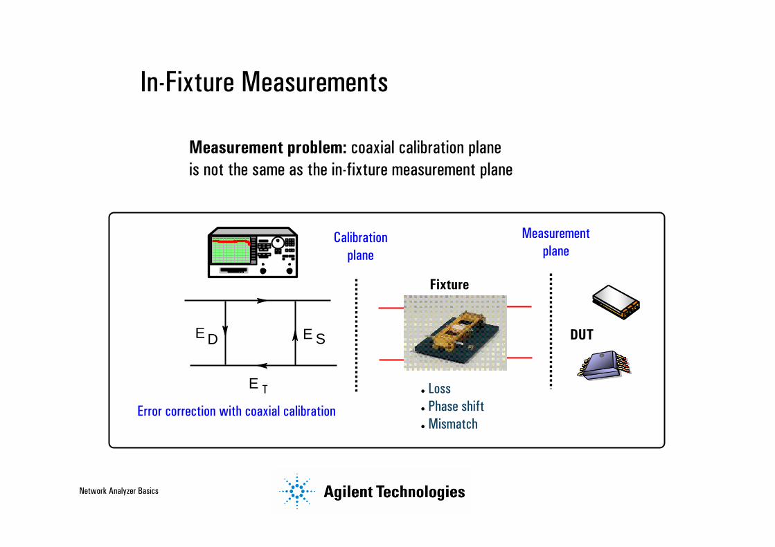
Measurement problem: coaxial calibration plane is not the same as the in-fixture measurement plane

Error correction with coaxial calibration

E E

E

D S

T LossPhase shiftMismatch

Calibrationplane

Measurementplane

DUT

Fixture


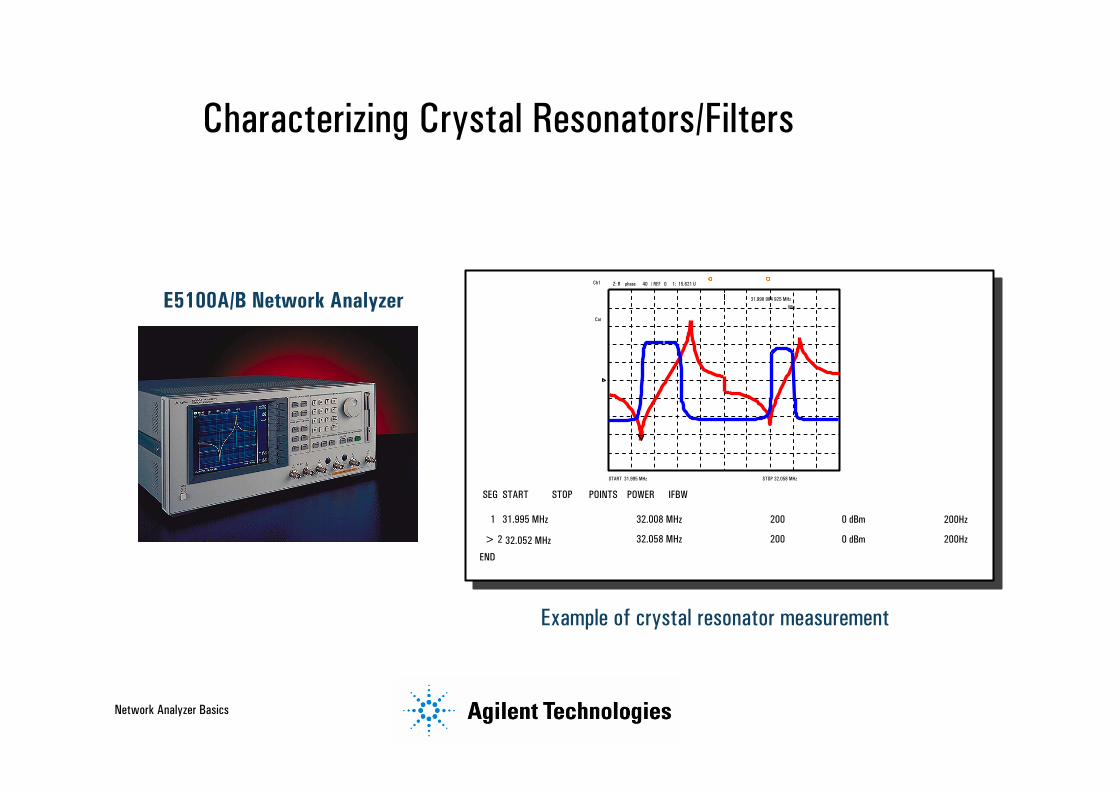
Characterizing Crystal Resonators/Filters

E5100A/B Network Analyzer

1 31.995 MHz

> 2

END

32.008 MHz

32.058 MHz

200

200

0 dBm

0 dBm

200Hz

200Hz

SEG START STOP POINTS POWER IFBW

32.052 MHz

Ch1

Cor

Z: R phase 40 / REF 0 1: 15.621 U

START 31.995 MHz STOP 32.058 MHz

31.998 984 925 MHz

Min

1

Example of crystal resonator measurement


What are Balanced Devices?Ideally, respond to differential and reject common-mode signals

Differential-mode signal

Common-mode signal

(EMI or ground noise)

Gain = 1

Differential-mode signal

Common-mode signal

(EMI or ground noise)

Gain = 1

Balanced to single-ended

Fully balanced


What about Non-Ideal Devices? Mode conversions occur...

+

Differential to common-mode conversion

Common-mode todifferential conversion

Generates EMI

Susceptible to EMI


So What?

RF and digital designers need to characterize:• Differential to differential mode (desired operation)• Mode conversions (undesired operation)• Operation in non-50-ohm environments• Other differential parameters:

– common-mode rejection ratio– K-factor– phase/amplitude balance– conjugate matches


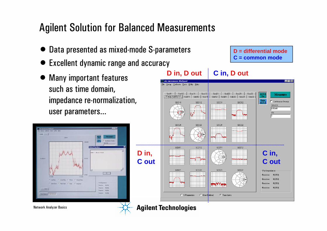
Agilent Solution for Balanced Measurements

• Data presented as mixed-mode S-parameters• Excellent dynamic range and accuracy

• Many important features such as time domain, impedance re-normalization, user parameters...

C in, D out

D in, C out

C in, C out

D in, D out

D = differential mode C = common mode


6 GHz Solution based on the PNA Series

Network Analyzer

Test Set

Software

• option 015 (allows standard VNA use)

• signal source• receiver

• adds 2 ports to VNA• includes switches, 2 couplers

• instrument control• calibration routines• error correction• measurement routines• “user” features• time domain

Optional 4-port ECal module


Target Markets

• Wireless Communications– Balanced topology less susceptible to EMI, noise– Less shielding required– RF grounding less critical– Better RF performance,

smaller, lighter phones– LVDS extends battery life

• Signal Integrity– Verify waveform quality of high speed digital signals– Engineers primarily interested in time-domain analysis


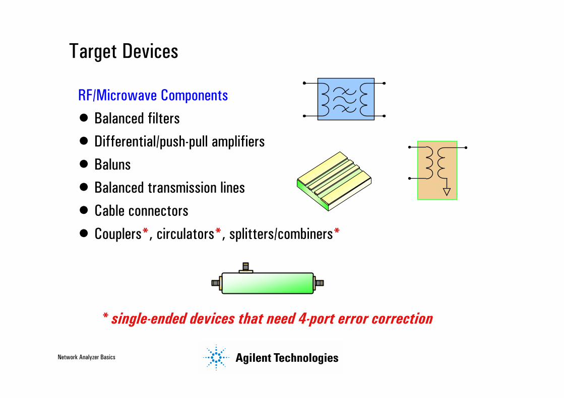
Target Devices

RF/Microwave Components• Balanced filters• Differential/push-pull amplifiers• Baluns• Balanced transmission lines• Cable connectors• Couplers*, circulators*, splitters/combiners*

* single-ended devices that need 4-port error correction


Target Devices

Digital Design• PCB backplanes• PCB interconnects• Sockets, packages• High-speed serial interconnects

(Ethernet, Firewire, Infiniband, USB …)


Agenda


Advanced Topicstime domain frequency-translating deviceshigh-power amplifiersextended dynamic rangemultiport devicesin-fixture measurementscrystal resonatorsbalanced/differential

Inside the network analyzerChallenge quiz!


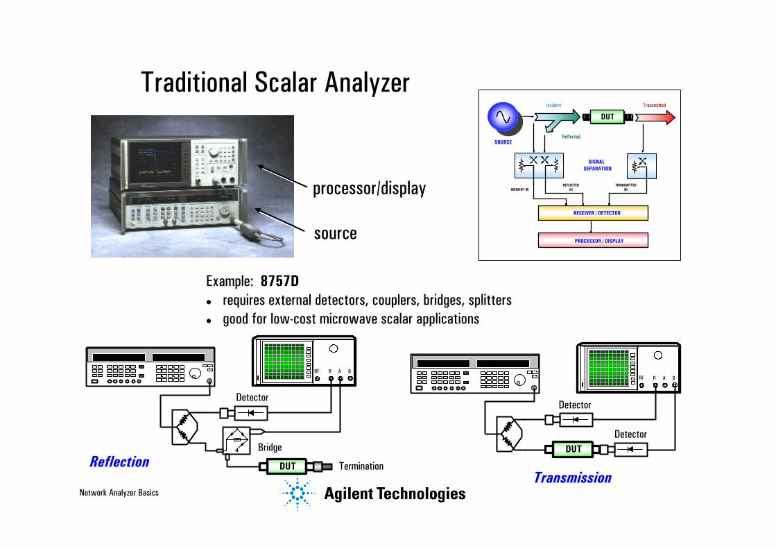
Traditional Scalar Analyzer

Example: 8757Drequires external detectors, couplers, bridges, splittersgood for low-cost microwave scalar applications

Detector

DUT

Bridge

TerminationReflectionTransmission

Detector

Detector

RF R A BRF R A B

DUT

processor/display

sourceRECEIVER / DETECTOR

PROCESSOR / DISPLAY

REFLECTED(A)


SIGNALSEPARATION

SOURCE

Incident

Reflected

Transmitted

DUT


Directivity = Coupling Factor (fwd) x Loss (through arm)

Isolation (rev)

Directivity (dB) = Isolation (dB) - Coupling Factor (dB) - Loss (dB)

Directional Coupler Directivity

Directivity = 50 dB - 30 dB - 10 dB = 10 dB

Directivity = 60 dB - 20 dB - 10 dB = 30 dB

10 dB

30 dB50 dB

10 dB

20 dB60 dB

Directivity = 50 dB - 20 dB = 30 dB

20 dB50 dB

Test port

Examples:

Test port

Test port


One Method of Measuring Coupler Directivity

Assume perfect load (no reflection)

short

1.0 (0 dB) (reference)

Coupler Directivity35 dB (.018)

Source

load

.018 (35 dB) (normalized)

Source

Directivity = 35 dB - 0 dB

= 35 dB


Directional Bridge

Test Port

Detector

50 Ω50 Ω

50 Ω

50-ohm load at test port balances the bridge -- detector reads zeroNon-50-ohm load imbalances bridgeMeasuring magnitude and phase of imbalance gives complex impedance"Directivity" is difference between maximum and minimum balance


RECEIVER / DETECTOR

PROCESSOR / DISPLAY

REFLECTED(A)


SIGNALSEPARATION

SOURCE

Incident

Reflected

Transmitted

DUT

NA Hardware: Front Ends, Mixers Versus Samplers

It is cheaper and easier to make broadband front ends using samplers instead of mixers

Mixer-based front end

ADC / DSPSampler-based front end

S

Harmonic generator

f

frequency "comb"

ADC / DSP


Mixers Versus Samplers: Time Domain

Single-balanced mixer (x1)

LORF

Sampler LO pulse

Mixer LO

Narrow pulse (easier to resolve noise)

Wide pulse (tends to average noise)

LORF

Sampler


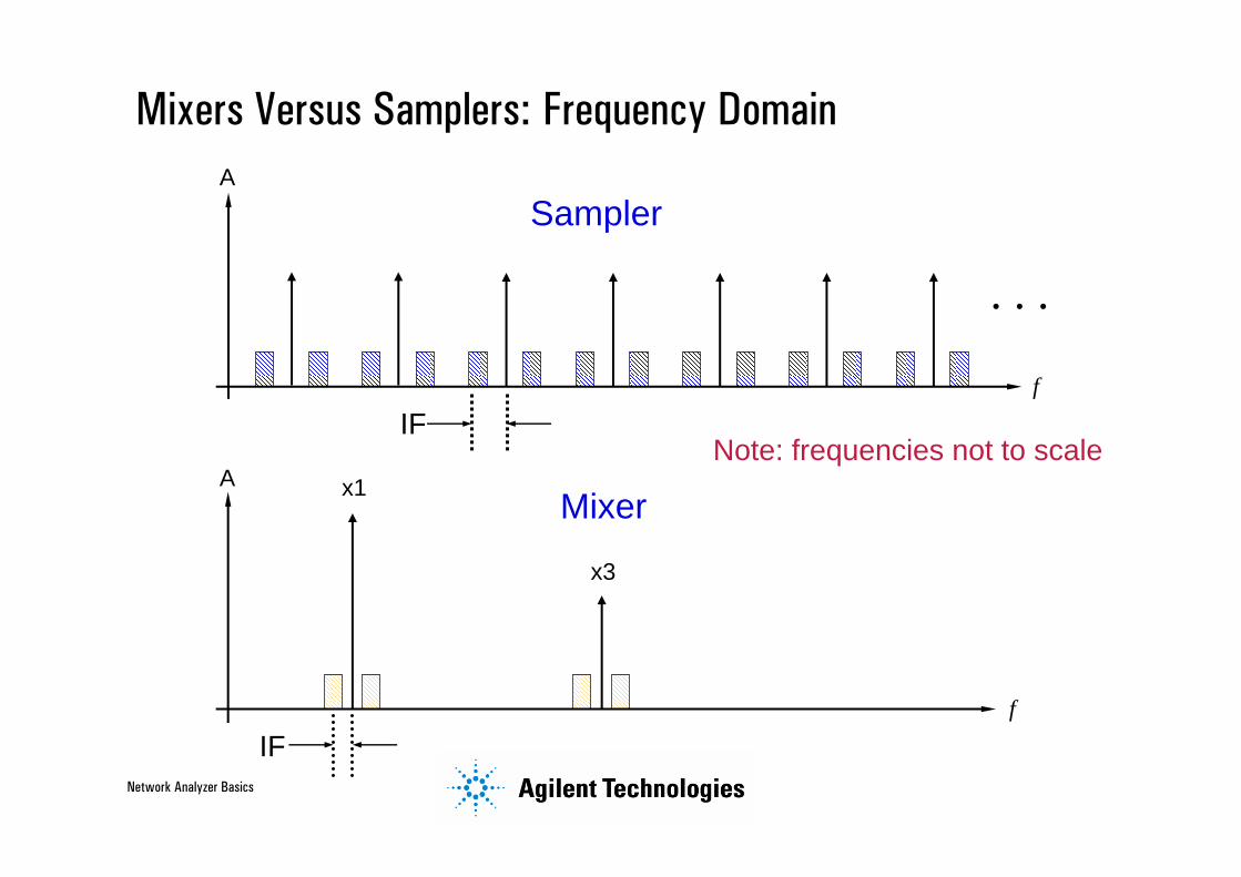
Mixers Versus Samplers: Frequency Domain

Note: frequencies not to scale

IF

x1

x3

f

Mixer

IF

. . .

f

SamplerA

A


Three Versus Four-Receiver Analyzers

Port 1

Transfer switch

Port 2

Source

B

R1

A

R2

Port 1 Port 2

Transfer switch

Source

B

R

A

3 receiversmore economicalTRL*, LRM* cals onlyincludes:

8753ES8720ES (standard)

4 receiversmore expensivetrue TRL, LRM calsincludes:

PNA Series8720ES (option 400)8510C


Why Are Four Receivers Better Than Three?

TRL TRL*

• 8720ES Option 400 adds fourth sampler, allowing full TRL calibration

• PNA Series has four receivers standard

TRL*assumes the source and load match of a test port are equal(port symmetry between forward and reverse measurements)this is only a fair assumption for three-receiver network analyzers

TRLfour receivers are necessary to make the required measurements TRL and TRL* use identical calibration standards

In noncoaxial applications, TRL achieves better source and load match correction than TRL*What about coaxial applications?

SOLT is usually the preferred calibration methodcoaxial TRL can be more accurate than SOLT, but not commonly used


Challenge Quiz1. Can filters cause distortion in communications systems?

A. Yes, due to impairment of phase and magnitude responseB. Yes, due to nonlinear components such as ferrite inductorsC. No, only active devices can cause distortionD. No, filters only cause linear phase shiftsE. Both A and B above

2. Which statement about transmission lines is false?A. Useful for efficient transmission of RF powerB. Requires termination in characteristic impedance for low VSWRC. Envelope voltage of RF signal is independent of position along lineD. Used when wavelength of signal is small compared to length of lineE. Can be realized in a variety of forms such as coaxial, waveguide, microstrip

3. Which statement about narrowband detection is false?A. Is generally the cheapest way to detect microwave signalsB. Provides much greater dynamic range than diode detectionC. Uses variable-bandwidth IF filters to set analyzer noise floorD. Provides rejection of harmonic and spurious signalsE. Uses mixers or samplers as downconverters


Challenge Quiz (continued)4. Maximum dynamic range with narrowband detection is defined as:

A. Maximum receiver input power minus the stopband of the device under testB. Maximum receiver input power minus the receiver's noise floorC. Detector 1-dB-compression point minus the harmonic level of the sourceD. Receiver damage level plus the maximum source output powerE. Maximum source output power minus the receiver's noise floor

5. With a T/R analyzer, the following error terms can be corrected:A. Source match, load match, transmission trackingB. Load match, reflection tracking, transmission trackingC. Source match, reflection tracking, transmission trackingD. Directivity, source match, load matchE. Directivity, reflection tracking, load match

6. Calibration(s) can remove which of the following types of measurement error?A. Systematic and driftB. Systematic and randomC. Random and driftD. Repeatability and systematicE. Repeatability and drift


Challenge Quiz (continued)7. Which statement about TRL calibration is false?

A. Is a type of two-port error correctionB. Uses easily fabricated and characterized standardsC. Most commonly used in noncoaxial environmentsD. Is not available on the 8720ES family of microwave network analyzersE. Has a special version for three-sampler network analyzers

8. For which component is it hardest to get accurate transmission and reflection measurements when using a T/R network analyzer?

A. Amplifiers because output power causes receiver compressionB. Cables because load match cannot be correctedC. Filter stopbands because of lack of dynamic rangeD. Mixers because of lack of broadband detectorsE. Attenuators because source match cannot be corrected

9. Power sweeps are good for which measurements?A. Gain compressionB. AM to PM conversionC. Saturated output powerD. Power linearityE. All of the above


Answers to Challenge Quiz

1. E2. C3. A4. B5. C6. A7. D8. B9. E

Network Analyzer Basics - index-of.co.ukindex-of.co.uk/Tutorials/network_analyzer_basics.pdf ·...

Documents

Transcript of Network Analyzer Basics - index-of.co.ukindex-of.co.uk/Tutorials/network_analyzer_basics.pdf ·...