NET GREENHOUSE GAS EMISSIONS AT EASTMAIN 1 …

1

NET GREENHOUSE GAS EMISSIONS AT EASTMAIN 1 RESERVOI R , QUEBEC,

CANADA

Alain Tremblay, Julie Bastien, Marie-Claude Bonneville, Paul del Giorgio, Maud Demarty, Michelle Garneau, Jean-Francois Hélie, Luc Pelletier, Yves Prairie,

Nigel Roulet, Ian Strachan, Cristian Teodoru.

ABSTRACT Growing concern over the long-term contribution of freshwater reservoirs to increased atmospheric concentration of greenhouse gases (GHGs) led Hydro-Québec to study net GHG emissions from Eastmain 1 reservoir. These are the emissions resulting from reservoir creation accounting for GHG produced or absorbed by the natural systems over a 100-year period for the watershed as a whole. This large-scale study was carried out in collaboration with the Université du Québec à Montréal, McGill University and Environnement IIlimité Inc. Gross GHG fluxes were measured using different techniques (eddy covariance, chambers, gas, partial pressure, etc.) for both aquatic and terrestrial ecosystems. More than 120,000 measurements were done over 7 years. The data clearly showed that, prior to flooding, the natural ecosystems overall were a low net source of CO2 and CH4. Net GHG emissions from Eastmain 1 increased following impoundment and quickly decreased, with a first-order exponential decay as net emissions would likely stabilized around 10 years after flooding. Diffusive fluxes dominate, with degassing and bubbling emissions representing less than 1% of total emissions. CH4 emissions are very small and represent less than 1% of total emissions. Overall net GHG emissions from Eastmain 1 reservoir are low in comparison with those from a thermal power plant of the same capacity (about 16%) and would be lower when extrapolated to the entire watershed.

RÉSUMÉ L'intérêt croissant en regard de la contribution des réservoirs à l'augmentation de la concentration des gaz à effet de serre (GES) dans l'atmosphère a amené Hydro-Québec à étudier les émissions nettes de GES au réservoir Eastmain 1. Les émissions nettes sont les émissions émises par le réservoir en considérant celles qui auraient été émises ou absorbées par les milieux naturels à l'échelle du bassin versant et sur une période de 100 ans et. Cette étude d'envergure est réalisée en collaboration avec l'Université du Québec à Montréal, McGill University et Environnement Illimité Inc. Les flux bruts furent mesurés avec différentes techniques (eddy covariance, chambres, pression partielle des gaz, etc.) tant dans les milieux aquatiques que terrestres. Plus de 120 000 mesures ont été réalisées sur une période de 7 ans. Les résultats démontrent clairement que les milieux naturels avant l'ennoiement étaient globalement une source faible de CO2 et de CH4. Les émissions nettes du réservoir EM-1 ont augmenté suivant la mise en eau et ont diminué rapidement suivant une courbe exponentielle du premier degré et tout semble indiquer que les émissions se stabiliseront après environ 10 ans. Les émissions sont dominées par les flux diffusifs, le dégazage et l'ébullition représentent moins de 1% des émissions. Les émissions de CH4 sont très faibles et représentent moins de 1% des émissions totales. Globalement, les émissions nettes de GES du réservoir Eastmain 1 sont faibles en comparaison des émissions d'une centrale thermique de capacité équivalente (environ 16%) et seraient plus petites lorsqu'extrapolées à l'échelle du bassin versant.

World Energy Congress, Montréal, September 12 to 16, 2010

2

1. INTRODUCTION

Lakes, rivers and wetlands, as well as reservoirs, are overall sources of greenhouse gases (GHGs) (Tremblay et al. 2005, Cole et al. 2007, Tranvik et al. 2009). The greenhouse effect is crucial for life on Earth, as it contributes to maintaining a mean annual temperature of about 15oC. However, over the last two decades, the rate of increase of anthropogenic GHG emissions to the atmosphere has reached a critical level. In Canada, hydropower plants represent about 60% of electricity generation capacity. It is generally recognized that boreal run-of-river power plants do not emit GHGs and that hydropower plants with reservoirs have low gross GHG emissions, in the order of 40 to 100 times less per terawatt/hour than those from thermal power plants (Tremblay et al. 2005). Nevertheless, the contribution of freshwater reservoirs to the increase in GHGs in the atmosphere is of growing concern (e.g., St. Louis et al. 2000, Tremblay et al. 2005).

The major GHGs related to reservoir creation are carbon dioxide (CO2), methane (CH4) and nitrous oxide (N2O) (Eggletion et al. 2006). Water residence time, reservoir shape and volume, and amount and type of vegetation flooded are variables that affect the duration and quantity of emissions (Tremblay et al. 2005). N2O emissions from reservoirs are typically very low, unless there are significant sources of nitrogen from the watershed (e.g., Tremblay et al. 2005, Eggletion et al. 2006).

Most of the data available in the literature only account for gross emissions measured at the

surface of water bodies and from established reservoirs (>10 years old; e.g., Tremblay et al. 2005, Bastien et al. 2009). Net emissions are emissions resulting from reservoir creation accounting for GHG produced or absorbed by the natural systems over a 100-year period for the watershed as a whole (IPCC, 2006, UNESCO-IHA, 2009). For governments and the energy sector, the evaluation of net GHG emissions from hydroelectric reservoirs is becoming more and more relevant to ensure that methods of energy production are compared adequately and for assessing CO2 credits. This is the goal of the Eastmain 1 net GHG emissions project (www.eastmain1.org) carried out in collaboration with the Université du Québec à Montréal, McGill University and Environnement Illimité Inc. The objective of this paper is to present net GHG emissions from Eastmain 1 reservoir, a world first. 2. SITE DESCRIPTION AND METHODOLOGY 2.1 Site Description

Eastmain 1 reservoir is located in the boreal ecoregion of Québec, Canada at 52°N, about 1,000 km north of Montréal (Figure 1). The watershed of the Eastmain region is dominated by coniferous forest, shallow podzolic and peat soils developed over igneous bedrock and quaternary sediments. Aquatic systems are described as oligotrophic with overall low primary production. The Eastmain-1 powerhouse is equipped with three turbines generating 160 MWh each, for a total of 480 MWh, and was commissioned in 2006. The main dam, along with 33 dikes, form the Eastmain 1 reservoir with a surface area of 603 km2. An additional 780 MWh will be available by 2012 with the construction of the Eastmain-1A powerhouse, yielding a total energy output from the Eastmain 1 reservoir of about 6.9 TWh per year (from 2012 and on). The hydrology of the Eastmain 1 reservoir basin (35,500 km2) reflects the regional climate; runoff is strongly seasonal


3

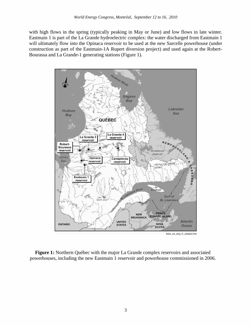
with high flows in the spring (typically peaking in May or June) and low flows in late winter. Eastmain 1 is part of the La Grande hydroelectric complex: the water discharged from Eastmain 1 will ultimately flow into the Opinaca reservoir to be used at the new Sarcelle powerhouse (under construction as part of the Eastmain-1A Rupert diversion project) and used again at the Robert-Bourassa and La Grande-1 generating stations (Figure 1).

Figure 1: Northern Québec with the major La Grande complex reservoirs and associated powerhouses, including the new Eastmain 1 reservoir and powerhouse commissioned in 2006.


4

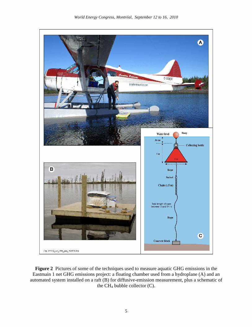
2.2 AQUATIC FLUX MEASUREMENTS AND CALCULATION The natural aquatic ecosystem is divided into three main categories: river, lakes and streams. Stretching over 138 km within the reservoir area, this section of the Rivière Eastmain covers an area of 82 km2. Accounting for 55% of the total aquatic surface area, the Rivière Eastmain represents the dominant areal component of the natural aquatic system in the region. Up to 827 lakes contained within the reservoir, with areas between 100 m2 and 10 km2, account for 45% of the total aquatic surface. Similarly, 827 streams of various sizes and lengths, from only 10 m up to 5.5 km and totaling 1.3 km2, represent the smallest areal component (less than 1%) of the natural aquatic system. There are three pathways by which a reservoir may emit GHGs: 1) diffusive emissions, measured at the water-air interface, 2) bubble emissions (mainly CH4), produced at the sediment-water interface and rising to the water-air interface, and 3) degassing or downstream emissions associated with turbulence at the turbines and spillway outflows (e.g. Tremblay et al. 2005). These three pathways were investigated at Eastmain 1 reservoir. Diffusive fluxes from the aquatic systems were measured using four different techniques: floating chamber, gas partial pressure, four automated systems and one eddy covariance tower located on Île Marie-Ève (Figure 2). More than 150 stations were spread over natural lakes, rivers, the new Eastmain 1 reservoir (one to four years old) and the old Opinaca reservoir (>30 years old) using the floating chamber and gas partial pressure techniques to determine the spatial and temporal variability of GHG emissions (Figure 3). One automated system was installed at Eastmain-1 powerhouse and three were installed on rafts on Eastmain 1 reservoir and on a reference lake. They were visited either by hydroplane or by boat. Sampling was conducted mainly during the ice-free season (May to October) but we also sampled, to a lesser extent, during winter (December to March) to calculate the GHG concentration increase under ice and an annual GHG flux (from ice melting to ice buildup) (Demarty et al. 2009). Diffusive fluxes were measured from 2003 to 2009 both from reference lakes and rivers (outside the present reservoir) and from lakes and rivers that are now part of Eastmain 1 reservoir (three years before flooding). Measurements on Eastmain 1 reservoir were carried out from June 2006 to October 2009 (four years after flooding).

To calculate fluxes, equations such as gas solubility in water, Henry's law, the Thin Boundary Layer equation, gas transfer coefficient and a series of secondary equations were used, according to the respective technique. Details on the techniques, equations and calculations can be found in Lambert and Fréchette (2005), Demarty et al. (2009), Tremblay et al. (2010) and Teodoru et al. (2009). Annual emissions were estimated from summer fluxes, considering an average ice-free period of 215 days and assuming that the buildup of C pool accumulated under the ice, which quickly decreases within the first month following ice breakup, represents approximately 30% of annual emissions as suggested by CO2 partial pressure data (Demarty et al. 2009, Ducharme-Riel et al. 2009).


5

Figure 2 Pictures of some of the techniques used to measure aquatic GHG emissions in the Eastmain 1 net GHG emissions project: a floating chamber used from a hydroplane (A) and an

automated system installed on a raft (B) for diffusive-emission measurement, plus a schematic of the CH4 bubble collector (C).


6

Degassing emissions were measured using a continuous gas monitor installed at the Eastmain-1 powerhouse from September 2006 to December 2009. The advantage of such an instrument is that it provides, with a single sampling station, a robust time series data set that is representative of the whole reservoir (Demarty et al. 2009). In order to estimate degassing fluxes, it was assumed that the concentration of CH4 and CO2 in the air was constant, that any gas concentration in the water exceeding that in the air was emitted into the air, and that the difference between both concentrations represents the degassing emissions that take place immediately downstream of the powerhouse. Details on equations and calculations are available in Demarty et al. (2009) or UNESCO-IHA (2009). This is considered to be a conservative estimate of degassing since, under natural conditions, the concentration of CH4 and CO2 in water is often oversaturated compared with its concentration in air. Annual overall degassing emissions were estimated by multiplying the monthly mean concentration of CH4 or CO2 in the water by the monthly mean water flow and factoring in the monthly mean water temperature, as temperature affects gas solubility in water.

Bubble emissions of CH4 were measured using bubble traps submerged (inverted funnels) at 30 cm beneath the water surface (Figure 2). The accumulated gas was sampled every two to three weeks from early June to late September 2008 and analyzed for CH4 concentration with a gas chromatograph. A total of 50 funnels were installed along eight transects of 5 to 10 funnels each, covering the four major pre-flooding cover types (forests, peatlands, lake and river) flooded by the Eastmain 1 reservoir (Figure 3). One transect was located on Lac Mitsumis, a reference lake. Low CH4 production was anticipated in the oligotrophic boreal waters studied. To estimate annual overall gross CH4 bubble emissions from the Eastmain 1 reservoir, the CH4 bubbling value was multiplied by the surface area of the reservoir, using 1% of 603 km2 for the lower limit of the extrapolated results, 5% for the mean value and 10% for the upper limit.

The carbon sink at the bottom of the Eastmain 1 reservoir, was estimated from 14 sedimentation traps installed at various locations within the reservoir from early June to the end of September in 2008 and from 24 sedimentation traps installed in 2009 (Figure 4). The natural variability in lakes was estimated from both sediment cores and sedimentation trap data collected from 11 various-size lakes located in the immediate vicinity of the reservoir. Details on these techniques can be found in Teodoru et al. (2010). The mean value of the carbon storage corresponds to the area-weighted averages from high sedimentation stations (5) and low sedimentation stations (9). The lower limit corresponds to the lowest carbon accumulation in sedimentation traps and the upper limit, to the highest accumulation rates.


7

Figure 3: Example of the sampling stations location in the Eastmain 1 area (Québec, Canada) for diffusive and bubble emission measurements. Degassing emissions were measured at Eastmain-1 powerhouse. Diffusive emissions were also measured

with automated systems and an eddy covariance system. Terrestrial fluxes were measured with eddy covariance and chamber techniques.


8

Figure 4 Picture and schematic of a sedimentation trap used in the Eastmain 1 net emissions project to estimate the carbon sink at the bottom of the Eastmain 1 reservoir

(Teodoru et al. 2010).

2.3 TERRESTRIAL FLUX MEASUREMENTS AND CALCULATION The natural terrestrial ecosystem is divided into two main categories: wetlands and forests. The forest can be divided into three types: coniferous forest represents the largest surface area, with 167 km2 or 49% of the total terrestrial surface area, while deciduous forest and burned forest respectively represent 16 km2 and 114 km2, and 5% and 33% of the surface area. Wetlands can be separated into three types: bogs represent 85 km2 or 14% of the total terrestrial surface area, and fens and wetlands-marsh-swamps respectively represent 1 km2 and 25 km2, and 0.2% and 4% of the surface area. The rest of the terrestrial surface area is occupied by bare soils that represent 46 km2 or 8% of the terrestrial surface area. No emissions were calculated from bare areas.


9

2.3.1 Forest Forest CO2 fluxes were estimated based on the net ecosystem exchange (NEE) measured from August 2006 in a mature and regionally representative black spruce forest (closed canopy located at Ian Tower on Figures 3 and 5) using eddy covariance (Figure 5). Net CO2 fluxes were measured 10 times per sec (10 Hz, 5 Hz during winter) and 30-minute averages were used in subsequent processing of the data. After quality control, gaps in the data were filled in using different techniques, taking into account ecosystem respiration, photosynthetically active radiation (PAR), soil temperature and other parameters. Details on the technique, equations and calculations are available in Baldocchi (2003) and Bonneville et al. (2007). These gap-filling methods are the standard procedures, used by the flux community in applying the eddy covariance technique (e.g. Barr et al. 2004). An overall annual CO2 budget was calculated by accumulating the NEE over each year of study. Since it is recognized, that the fire cycle is around 100 years (Mansey et al. submitted), 1% of the landscape, on average, should burn yearly. Therefore, we assumed that about 1% of the total burnable area (coniferous+deciduous+burned area), which represents 3 km2, would burn every year and that 50% of the related biomass burned would be emitted to the atmosphere as CO2.

In order to compute the regional coniferous forest CO2 budget, NEE values measured at Eastmain 1 were combined with literature data from other representative boreal black spruce forests of different ages and jack pine forests. In this way, we could take into account the spatial and temporal variability in NEE for the different coniferous forest types. For deciduous forests, the CO2 budget was derived from literature data on eddy covariance NEE measurements made in boreal aspen forests. Literature data were used to estimate the CO2 budget of burned forests.

Forest CH4 fluxes were estimated from chamber measurements of soil CH4 fluxes taken in 2007 in regionally representative coniferous, deciduous and burned forest sites in the reservoir surroundings. Fluxes were determined based on linear change in gas concentration from samples collected over a 90-min period and analyzed on a gas chromatograph (Ullah et al. 2009).


10

Figure 5 Pictures of some of the techniques used to measure terrestrial GHG fluxes in the Eastmain 1 net GHG emissions project: an eddy covariance tower at Ian tower site (A)

and in the Lac Le Caron peatlands (B), and clear terrestrial chambers (C).


11

Fluxes of CH4 were measured six times between June and October 2007. Annual fluxes were estimated by multiplying daily average growing season values by the length of the growing season (determined by eddy covariance tower data) and assuming no winter fluxes. The forest CO2 and CH4 budget was calculated as the area-weighted sum of the CH4 budget for each forest type (coniferous, deciduous and burned). 2.3.2 Wetlands

Peatlands chamber measurements of NEE-CO2 and CH4 fluxes were performed in six regionally representative bogs (figures 3 and 5) between 2005 and 2009, and in fens from 2006 to 2008. Fluxes were measured from five different microforms (high hummocks, low hummocks, hollows, lawns, pools) representative of the spatial heterogeneity of the peatlands. Sampling was done during the growing season (from May to October). Wintertime daily average fluxes were assumed to be 10% of the growing season fluxes (Pelletier et al. 2007, Pelletier 2005). Growing season fluxes, PAR and other parameters were used to estimate overall annual fluxes. Details on the techniques, equations and calculations are available in Pelletier et al. (2009), Pelletier et al. (2007) and Bonneville et al. (2009).

From June 2008 to December 2009, NEE-CO2 was also measured directly with a portable eddy covariance tower located in the Lac Le Caron peatlands (LLC, Figures 3 and 5). Data processing and annual CO2 budget calculation were performed similarly to those for the forest data. In summer 2009, a Los Gatos fast-methane analyzer was also used to measure CH4 fluxes in the Lac Le Caron peatlands with the flux gradient micrometeorological technique (Wagner-Riddle et al. 1996). Continuous CH4 concentrations measured at 1 Hz were obtained from two heights, and the resulting computed fluxes were averaged over 30 minutes.

The bog CO2 budget is an average of the fluxes measured for each year from 2006

to 2009 using the chamber data, and the average annual CO2 budget derived from the flux tower data collected in 2008 and 2009. The fen CO2 budget was obtained by averaging the chamber fluxes measured in 2006 and 2008. The overall regional wetland CO2 budget consists of the area-weighted sum of the CO2 and CH4 budget for each peatland type (bogs, fens), with swamps/marshes given the average value for all peatlands. 3. RESULTS AND DISCUSSION

According to the IPCC (2006) and UNESCO-IHA (2009) definition, net GHG emissions from a reservoir should be calculated over a 100-year period and for the watershed as a whole. However, to determine net emissions in the present analysis, we only consider the surface area flooded by the creation of the EM-1 reservoir. To calculate net GHG emissions at the Eastmain 1 reservoir, we considered the following elements: - Bubbles, degassing and diffusive emissions from Eastmain 1 reservoir are direct emissions from the reservoir and are related to reservoir creation.


12

- Sources of GHG emissions from natural ecosystems (lakes, rivers, streams, forest fire emissions, CH4 emissions from peatlands and carbon sedimentation in the reservoir) were subtracted from Eastmain 1 reservoir emissions.

- GHG sinks in natural ecosystems (forest and peatland CO2 sinks) were added to Eastmain 1 reservoir emissions.

- We used the data from natural ecosystems and reservoir data from four years after flooding to predict Eastmain 1 net GHG emissions over 100 years.

As it is very difficult to predict precise values over a long period of time, we are

presenting the long-term trends using three different scenarios: mean, lower limit and upper limit scenarios. The first uses the mean net emissions from the reservoir and corresponds to the post-flooding gross carbon emissions minus the area-weighted pre-flooding carbon emissions from the terrestrial and aquatic ecosystems. If the pre-flooding ecosystem was a net sink, then the resulting net reservoir effect will be larger than the gross emissions measured from the reservoir. The lower limit scenario (least net change from pre- to post-flooding, best-case scenario) uses the largest pre-flooding terrestrial carbon emissions (or smallest terrestrial carbon sink), the largest pre-flooding aquatic carbon emissions and the lowest values for diffusive, degassing and bubble emissions from the reservoir. The upper limit scenario (most net change from pre- to post-flooding, worst-case scenario) uses the smallest pre-flooding terrestrial carbon emissions (or largest terrestrial carbon sink), the smallest pre-flooding aquatic carbon emissions and the highest values for diffusive, degassing and bubble emissions from the reservoir. Negative values indicate a sink (absorption) of GHG and positive values indicate a source (emission) of GHG from the ecosystems.

Our results are based on more than 120,000 measurements taken over seven years. The data from natural ecosystems (aquatic and terrestrial ecosystems) showed that the ecosystems to be flooded, including forest fires, were overall a low net source of carbon, with a mean value of about 3,200 tonnes of C-CO2/year. The forests were net CO2 sinks for the mean and lower limit scenarios, with values ranging from -27,000 to −12,000 tonnes of C-CO2/year. The upper limit scenario showed a low carbon sink with a value of 1,200 tonnes of C-CO2/year. Peatlands/wetlands ecosystems showed the same trend with a lower sink or source of CO2, with values of -8,800, -4,200 and 600 tonnes of C-CO2/year for the lower limit, mean and upper limit scenarios, respectively. However, peatland/wetland were sources of CH4, with values ranging from 1,350 to 1,850 tonnes of C-CH4/year. On the other hand, all aquatic ecosystems, including ponds in the peatlands, were a source of CO2 and CH4, with values ranging from 525 to 13,300 tonnes of C-CO2/year and 23 to 102 tonnes of C-CH4/year. The contribution of streams to the C-CO2 source in natural aquatic ecosystems is substantial relative to their small total surface area. However, lakes’ carbon sedimentation represents a low sink, with values ranging from -250 to -1,255 tonnes of C-CO2/year.

Net Eastmain 1 emissions are changing over time, starting from very high in the

first year (500,000 tonnes of C-CO2) and decreasing exponentially over the following four years (165,000 tonnes of C-CO2) for the mean scenario. Eastmain 1 emissions are totally dominated by CO2 diffusive emissions, which represent more than 99% of total


13

emissions; therefore, degassing and bubbling emissions represent less than 1% of the total. Sedimentation at the bottom of the reservoir is about twice as much as in natural lakes but represents a small fraction of the total flux. CH4 emissions are very small and represent less than 1% of total emissions.

To predict the evolution of net CO2 fluxes over 100 years, we calculated the lower limit of gross CO2 fluxes from measurements taken on older reservoirs (ranging from 12 to 30 years old) in the same boreal region (Caniapiscau, La Grande 1, La Grande 3, La Grande 4, Laforge 1, Opinaca, Robert-Bourassa [Figure 1, Tremblay et al. 2005]) and combined them with the initial Eastmain 1 data to determine the long-term pattern in minimum CO2 emissions. We further assumed that the difference between upper limit, mean and lower limit values of net CO2 fluxes estimated for the first four years for Eastmain 1 reservoir will be maintained over time, and on this basis we estimated the potential range in net CO2 emissions over a 100-year period (Figure 6).

Figure 6: Evolution of Eastmain 1 net emissions (tonnes of carbon) over time (years) for

the lower limit (best-case scenario), mean and upper limit (worst-case scenario).


14

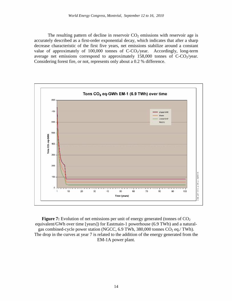
The resulting pattern of decline in reservoir CO2 emissions with reservoir age is

accurately described as a first-order exponential decay, which indicates that after a sharp decrease characteristic of the first five years, net emissions stabilize around a constant value of approximately of 100,000 tonnes of C-CO2/year. Accordingly, long-term average net emissions correspond to approximately 158,000 tonnes of C-CO2/year. Considering forest fire, or not, represents only about a 0.2 % difference.

Figure 7: Evolution of net emissions per unit of energy generated (tonnes of CO2 equivalent/GWh over time [years]) for Eastmain-1 powerhouse (6.9 TWh) and a natural-

gas combined-cycle power station (NGCC, 6.9 TWh, 380,000 tonnes CO2 eq./ TWh). The drop in the curves at year 7 is related to the addition of the energy generated from the

EM-1A power plant.


15

The model of net CO2 emissions from Eastmain 1 reservoir can be used to estimate the temporal evolution of CO2 equivalent emissions per unit of energy generated for the reservoir (Figure 7). For energy output of 6.9 TWh/year, net CO2 eq. emissions per unit of energy generated were initially relatively high, at about 640 tonnes of CO2 eq./GWh, but these annual emissions quickly decline and are below those from a natural-gas combined-cycle (NGCC) generating station after the initial three years (Tremblay et al. 2005). However, it takes about five years for the accumulated CO2 eq. emissions to fall below the NGCC value (Figure 8). Our model further predicts that these net emissions should stabilize at around 54 tonnes of CO2 eq./GWh after 10 years, and stay roughly constant at that level thereafter for the mean scenario.

Figure 8: Cumulative net GHG emissions per unit of energy generated (tonnes of CO2 equivalent/GWh over time [years]) for Eastmain-1 powerhouse (6.9 TWh ) and a natural-

gas combined-cycle power station (NGCC, 6.9 TWh, 380,000 tonnes CO2 eq./ TWh).


16

4. CONCLUSIONS

Our study has shown that natural ecosystems to be flooded were overall a low net source of carbon. Net GHG emissions are substantial in the first years after flooding and decrease rapidly, stabilizing after about 10 years. This study also clearly indicates that CH4 emissions, degassing and bubbling emissions are not significant in terms of net GHG emissions from Eastmain 1 and that they are probably not an issue in most boreal reservoirs.

With a relatively small surface area and a very short water residence time, for an installed capacity of about 1,250 MW, Eastmain 1 reservoir is a good example of a project emitting small amounts of GHGs. The most efficient thermal power plants, natural-gas combined-cycle, emit about 380,000 tonnes of CO2 equivalent per TWh (Tremblay et al. 2005), whereas Eastmain 1 reservoir emits 16% of this amount over a 100 year. If the results are extrapolated to the entire watershed, net emissions from Eastmain 1 would be even lower. These results clearly indicate that boreal hydroelectric reservoirs are low GHG emitters. Boreal hydropower plants should therefore be considered part of the solution to reduce the impact on climate change.

REFERENCES Baldocchi, D.D. 2003. Assessing the eddy covariance technique for evaluating carbon

dioxide exchange rates of ecosystems: past, present and future. Global Change Biol. 9, 479–492.

Barr, A.G., T.A. Black, E.H. Hogg, N. Kljun, K. Morgenstern and Z. Nesic. 2004. Inter-annual variability in the leaf area index of a boreal aspen-hazelnut forest in relation to net ecosystem production. Agric. Forest Meteorol. 126, 237–255.

Bastien, J., A. Tremblay and L. LeDrew. 2009. Greenhouse gas fluxes from Smallwood Reservoir and natural water bodies in Labrador, Newfoundland, Canada. Verh. Internat. Verein. Limnol. 30,6: 858-861.

Bonneville, M.-C., I.B. Strachan, E. Humphreys and N.T. Roulet. 2008. Net ecosystem CO2 exchange in a temperate cattail marsh in relation to biophysical properties. Agric. Forest Meteorol. Doi:10.1016/j.agrformet.20017.09.004.

Cole, J.J, Y.T. Prairie, N.F. Caraco, W.H. McDowell, L.J. Tranvik, R.G. Striegl, C.M. Duarte, P. Kortelainen, J.A. Downing, J.J. Middelburg and J. Melack. 2007. Plumbing the global carbon cycle: integrating inland waters into the terrestrial carbon budget. Ecosystems 10: 172-185.

Demarty, M., J. Bastien, A. Tremblay, R. Hesslein and R. Gill. 2009. Greenhouse Gas Emissions from Boreal Reservoirs in Manitoba and Québec, Canada, Measured with Automated Systems. Environmental Science and Technology 43,23: 8905-8915.

Eggletion, H.S., L. Buendia, K. Iwa, T. Ngara and K. Tanabe (eds.). 2006. Intergovernmental Panel on Climate Change (IPCC), National Greenhouse Gas


17

Inventories Guidelines, Vol. 4 – Agriculture, Forestry and Other Land Use. Kanagawa, Japan: IGES. AP2.1-AP2.9.

Intergovernmental Panel on Climate Change (IPCC). 2006. Climate change: the scientific basis. Contribution of Working Group I to the Third Assessment Report of the IPCC. New York: Cambridge University Press.

Kortelainen, P., J.T. Huttunen, T. Väisänen, T. Mattsson, P. Karjalainen and P.J. Martikainen. 2000. CH4, CO2 and N2O supersaturation in 12 Finnish lakes before and after ice-melt. Verh. Internat. Verein. Limnol. 27: 1410-1414.

Lambert, M. and J.-L. Fréchette. 2005. Analytical Techniques for Measuring Fluxes of CO2 and CH4 from Hydroelectric Reservoirs and Natural Water Bodies. In Tremblay, A., L. Varfalvy, C. Roehm and M. Garneau, (eds.). 2005. Greenhouse Gas Emissions: Fluxes and Processes, Hydroelectric Reservoirs and Natural Environments. Berlin, Heidelberg, New York: Springer-Verlag. P. 37-60.

Pelletier, L., M. Garneau and A. Tremblay. 2009. CO2 and CH4 ecosystem exchange from peatlands: Eastmain-1 hydro-electric project, Quebec, Canada. Verh. Internat. Verein. Limnol. 30,6: 862-865.

Pelletier, L. 2005. Carbon dioxide and methane fluxes of three peatlands in the La Grande Rivière watershed, James Bay lowland, Canada. M.Sc. thesis, McGill University, Montréal, Québec, Canada.

Pelletier, L., T. R. Moore, N. T. Roulet, M. Garneau and V. Beaulieu-Audy. 2007. Methane fluxes from three peatlands in the La Grande Rivière watershed, James Bay lowland, Canada. J. Geophys. Res. 112, G01018, doi:10.1029/2006JG000216.

St. Louis, V.L., C.A. Kelly, E. Duchemin, J.W.M. Rudd and D.M. Rosenberg. 2000. Reservoir surfaces as sources of greenhouse gases to the atmosphere: a global estimate. BioScience 50: 766-775.

Teodoru, C.R., P. del Giorgio, Y. Prairie and M. Camire. 2009. pCO2 dynamics in boreal streams of northern Quebec, Canada. Global Biogeochemical Cycles 23, GB2012, doi:10.1029/2008GB003404.

Teodoru, C.R., P. del Giorgio, Y. Prairie and A. St-Pierre. 2010. Particle deposition trends and carbon sources in a young boreal reservoir in northern Quebec relative to natural variability in lakes of the surrounding region. Submitted to Limnology & Oceanography.

Tranvik, L.J., J.A. Downing, J.B. Cotner, S. A. Loiselle, R. G. Striegl, T.J. Ballatore, P. Dillon, K. Finlay, K. Fortino, L.B. Knoll, P.L. Kortelainen, T. Kutser, S. Larsen , I. Laurion, D.M. Leech, S.L. McCallister, D.M. McKnight, J.M. Melack, E. Overholt, J.A. Porter, Y. Prairie, W.H. Renwick, F. Roland, B.S. Sherman, D.W. Schindler, S. Sobek, A. Tremblay, M.J. Vanni, E. von Wachenfeldt, E.D. Wachenfeldt, and G.A. Weyhenmeyer. 2009. Lakes and Reservoirs as Regulators of Carbon Cycling and Climate. Limnology and Oceanography 54,6 (part 2): 2298-2314.

Tremblay, A., M. Lambert and L. Gagnon. 2004. CO2 Fluxes from Natural Lakes and Hydroelectric Reservoirs in Canada. Environ. Manag. 33,1: S509-S517.

Tremblay, A., L. Varfalvy, C. Roehm and M. Garneau (eds.). 2005. Greenhouse gas emissions: fluxes and processes, hydroelectric reservoirs and natural environments. Berlin, Heidelberg, New York: Springer-Verlag.

Tremblay, A., L. Varfalvy and M. Lambert. 2008. Greenhouse Gases from Boreal Hydroelectric Reservoirs: 15 years of data ? Proceedings of 15th International


18

Seminar on Hydropower Plants, HydroPower Plants in the Context of the Climate Change. November 26-28, Conference Center Laxenburg, Vienna, Austria. P. 453-362.

Ullah, S., R. Frasier, L. Pelletier and T.R. Moore. 2008. Greenhouse gas fluxes from boreal forest soils during the snow-free period in Quebec, Canada. Soil Biology and Biochemistry 40: 986-994.

UNESCO-IHA, 2009. The UNESCO-IHA measurement specification guidance for evaluating the GHG status of man-made freshwater reservoirs. (http://www.hydropower.org/climate_initiatives/GHG-Measurement_Specification_Guide_Edition_1_June_2009.pdf)

Van Bellen, S., P.-L. Dallaire, M. Garneau and Y. Bergeron. 2010. Long-term spatial C accumulation patterns in ombrotrophic peatlands of the Eastmain region, Quebec, Canada. Submitted to Global Biogeochemical Cycles.

Wagner-Riddle, C., G.W. Thurtell, K.M. King, G.E. Kidd and E.G. Beauchamp. 1996. Nitrous oxide and carbon dioxide fluxes from a bare soil using a micrometeorological approach. J. Environ. Qual. 25: 898-907.

NET GREENHOUSE GAS EMISSIONS AT EASTMAIN 1 …

Documents

Transcript of NET GREENHOUSE GAS EMISSIONS AT EASTMAIN 1 …