Nested Logit - University of California, Davispsfaculty.ucdavis.edu/bsjjones/nestedlogit.pdf · I...

Nested Logit

Brad Jones1

1Department of Political ScienceUniversity of California, Davis

April 30, 2008

Jones POL 213: Research Methods

Nested Logit

I Interesting model that does not have IIA property.

I Possible candidate model for structured choice situations.

I Conceptual example:

I J political parties a voter i could choose from.

I Say: Green, Workers, Social Dem., Moderate, CR, ExtremeRight

I Models?

I Conditional logit or MNL?

I IIA property could be an issue.


Nested Logit

I IIA “says” that the disturbances are independent andhomoskedastic.

I Odds are assumed to remain the same if some alternative isremoved.

I Problem: one left party is a close substitute (possibly) ofanother.

I If CD voters split their vote across two leftist parties,elimination of one from the choice set does not imply they willrandomly distribute over remaining choices.

I That is, they most likely will gravitate to the remaining leftistparty.

I If so, odds ratios will change because of nonrandomredistribution.


Nested Logit

I Under NL (or MNNL), the idea is to group comparablealternatives and then structure choice setting as a “tree.”

I Voter i decides to vote leftist, centrist, or rightist.

I Call this the “top level” choice.

I Once this choice is made, the voter must decide whichoutcome to choose:

I Left: Green, Workers; Center: SD, Moderate; Right: CR,Extreme Right

I Basic result from conditional probability: Prij = Prj |i ×PriI J outcomes (i.e. parties) and i branches.


Nested Logit

I Conditional probability says the probability of the “bottomlevel” choice is equal to the conditional probability of selectingj given branch i times the probability that branch i wasselected.

I ∃ two levels of probability because ∃ two levels of decisions.

I Consider the conditional probability statement, Prj |i .

I Suppose we specify a utility model:

Uij = β′xij + α′wi

I As in the CL presentation, the xij are covariates that canchange over the choices (bottom level) and the wi arecovariates that are attributes of the choice sets (top level).


Nested Logit

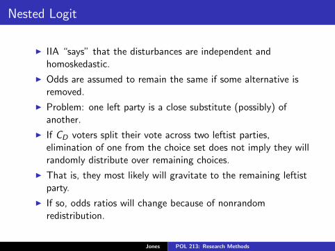
I The conditional probabilities can only be a function of the xij :

Prj |i =exp(β′xij) exp(α′wi )

exp(α′wi )∑Ni

k=1 exp(β′xik)

=exp(β′xij)∑Ni

k=1 exp(β′xik)

I The “top level” probability is defined by first identifying whatis sometimes called an “inclusive value” parameter:

Ii = log

(Ni∑

k=1

exp(β′xik)

)I The probability of branch i is then

Pri =exp(α′wi + τi Ii )∑C

m=1 exp(α′wi + τmIm)


Nested Logit

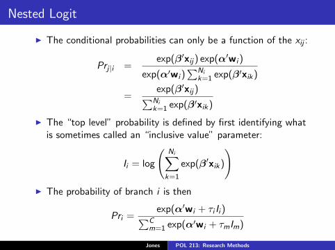
I The “inclusive value” parameter, τ , is the weight accordedeach of the branches.

I Under CL (or MNL), we assume this weight is fixed at 1.

I Estimation is done via full information maximum likelihood:

log L =N∑i

log[Prj |i × Pri

].

I Model has many parameters.

I It requires a lot of work to interpret.

I My job to show you how . . .

I Stata is actually quite good w/this model.


Nested Logit: Illustration

I I’m going to continue with the Stata data set provided bytheir website.

I We used it with conditional logit.

I Let’s consider the data structure.


. list family_id restaurant chosen kids rating distance cost income in 1/21

+---------------------------------------------------------------------------------+

| family~d restaurant chosen kids rating distance cost income |

|---------------------------------------------------------------------------------|

1. | 1 Freebirds 1 1 0 1.245553 5.444695 39 |

2. | 1 MamasPizza 0 1 1 2.82493 6.19446 39 |

3. | 1 CafeEccell 0 1 2 4.21293 8.182085 39 |

4. | 1 LosNortenos 0 1 3 4.167634 9.861741 39 |

5. | 1 WingsNmore 0 1 2 6.330531 9.667909 39 |

|---------------------------------------------------------------------------------|

6. | 1 Christophers 0 1 4 10.19829 25.95777 39 |

7. | 1 MadCows 0 1 5 5.601388 28.99846 39 |

8. | 2 Freebirds 0 3 0 4.162657 5.26874 58 |

9. | 2 MamasPizza 0 3 1 2.865081 5.728618 58 |

10. | 2 CafeEccell 0 3 2 5.337799 7.054855 58 |

|---------------------------------------------------------------------------------|

11. | 2 LosNortenos 1 3 3 4.282864 10.78514 58 |

12. | 2 WingsNmore 0 3 2 8.133914 8.313948 58 |

13. | 2 Christophers 0 3 4 8.664631 21.2801 58 |

14. | 2 MadCows 0 3 5 9.119597 25.87567 58 |

15. | 3 Freebirds 1 3 0 2.112586 4.616315 30 |

|---------------------------------------------------------------------------------|

16. | 3 MamasPizza 0 3 1 2.215329 5.992166 30 |

17. | 3 CafeEccell 0 3 2 6.978715 7.980528 30 |

18. | 3 LosNortenos 0 3 3 5.117877 10.0605 30 |

19. | 3 WingsNmore 0 3 2 5.312941 8.76644 30 |

20. | 3 Christophers 0 3 4 9.551273 23.64499 30 |

|---------------------------------------------------------------------------------|

21. | 3 MadCows 0 3 5 5.539806 24.72128 30 |

+---------------------------------------------------------------------------------+


. nlogitgen type=restaurant(fast: Freebirds | MamasPizza,

family: CafeEccell | LosNortenos | WingsNmore, fancy: Christophers | MadCows)

This returns:

new variable type is generated with 3 groups

label list lb_type

lb_type:

1 fast

2 family

3 fancy

. nlogittree restaurant type <-GIVES US THE TREE STRUCTURE.

Type is the branch; restaurants are the "twigs."

tree structure specified for the nested logit model

top --> bottom

type restaurant

--------------------------

fast Freebirds

MamasPizza

family CafeEccell

LosNorte~s

WingsNmore

fancy Christop~s

MadCows


\newpage

. nlogit chosen (restaurant= cost rating distance)

(type = incFast incFancy kidFast kidFancy), group(family_id) nolog

Nested logit estimates

Levels = 2 Number of obs = 2100

Dependent variable = chosen LR chi2(10) = 199.6293

Log likelihood = -483.9584 Prob > chi2 = 0.0000

------------------------------------------------------------------------------

| Coef. Std. Err. z P>|z| [95% Conf. Interval]

-------------+----------------------------------------------------------------

restaurant |

cost | -.0944352 .03402 -2.78 0.006 -.1611131 -.0277572<-These are the alpha parms.

rating | .1793759 .126895 1.41 0.157 -.0693338 .4280855

distance | -.1745797 .0433352 -4.03 0.000 -.2595152 -.0896443

-------------+----------------------------------------------------------------

type |

incFast | -.0287502 .0116242 -2.47 0.013 -.0515332 -.0059672 <-WHY DO I HAVE THESE?

incFancy | .0458373 .0089109 5.14 0.000 .0283722 .0633024 <-These are the beta parms.

kidFast | -.0704164 .1394359 -0.51 0.614 -.3437058 .2028729

kidFancy | -.3626381 .1171277 -3.10 0.002 -.5922041 -.1330721

-------------+----------------------------------------------------------------

(incl. value |

parameters) |

type |

/fast | 5.715758 2.332871 2.45 0.014 1.143415 10.2881 <-These are the tau parms.

/family | 1.721222 1.152002 1.49 0.135 -.5366608 3.979105

/fancy | 1.466588 .4169075 3.52 0.000 .6494642 2.283711

------------------------------------------------------------------------------

LR test of homoskedasticity (iv = 1): chi2(3)= 9.90 Prob > chi2 = 0.0194

------------------------------------------------------------------------------


For fun.

. nlogit chosen (restaurant= cost rating distance) (type = incFast

incFancy kidFast kidFancy), group(family_id)

nolog ivc(fast=1, family=1, fancy=1) notree <---CONSTRAINING TAU TO 1

User-defined constraints:

IV constraints:

[fast]_cons = 1

[family]_cons = 1

[fancy]_cons = 1

Nested logit regression




------------------------------------------------------------------------------


-------------+----------------------------------------------------------------

restaurant |

cost | -.1367799 .0358479 -3.82 0.000 -.2070404 -.0665193

rating | .3066626 .1418291 2.16 0.031 .0286827 .5846424

distance | -.1977508 .0471653 -4.19 0.000 -.2901931 -.1053085

-------------+----------------------------------------------------------------

type |

incFast | -.0390182 .0094018 -4.15 0.000 -.0574454 -.020591

incFancy | .0407053 .0080405 5.06 0.000 .0249462 .0564644

kidFast | -.2398756 .1063674 -2.26 0.024 -.4483517 -.0313994

kidFancy | -.3893868 .1143797 -3.40 0.001 -.6135669 -.1652067

-------------+----------------------------------------------------------------

(incl. value |

parameters) |

type |

/fast | 1 . . . . .

/family | 1 . . . . .

/fancy | 1 . . . . .

------------------------------------------------------------------------------


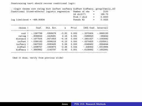
Constraining tau=1 should recover conditional logit:

. clogit chosen cost rating dist incFast incFancy kidFast kidFancy, group(family_id)

Conditional (fixed-effects) logistic regression Number of obs = 2100

LR chi2(7) = 189.73

Prob > chi2 = 0.0000

Log likelihood = -488.90834 Pseudo R2 = 0.1625

------------------------------------------------------------------------------

chosen | Coef. Std. Err. z P>|z| [95% Conf. Interval]

-------------+----------------------------------------------------------------

cost | -.1367799 .0358479 -3.82 0.000 -.2070404 -.0665193

rating | .3066622 .1418291 2.16 0.031 .0286823 .584642

distance | -.1977505 .0471653 -4.19 0.000 -.2901927 -.1053082

incFast | -.0390183 .0094018 -4.15 0.000 -.0574455 -.0205911

incFancy | .0407053 .0080405 5.06 0.000 .0249462 .0564644

kidFast | -.2398757 .1063674 -2.26 0.024 -.448352 -.0313994

kidFancy | -.3893862 .1143797 -3.40 0.001 -.6135662 -.1652061

-----------------------------------------------------------------------------

(And it does; verify from previous slide)


But since we know IIA doesn’t hold, we should continue with unconstrained

nested logit.

Nested logit regression




------------------------------------------------------------------------------


-------------+----------------------------------------------------------------

restaurant |

cost | -.0944352 .03402 -2.78 0.006 -.1611131 -.0277572

rating | .1793759 .126895 1.41 0.157 -.0693338 .4280855

distance | -.1745797 .0433352 -4.03 0.000 -.2595152 -.0896443

-------------+----------------------------------------------------------------

type |

incFast | -.0287502 .0116242 -2.47 0.013 -.0515332 -.0059672

incFancy | .0458373 .0089109 5.14 0.000 .0283722 .0633024

kidFast | -.0704164 .1394359 -0.51 0.614 -.3437058 .2028729

kidFancy | -.3626381 .1171277 -3.10 0.002 -.5922041 -.1330721

-------------+----------------------------------------------------------------

(incl. value |

parameters) |

type |

/fast | 5.715758 2.332871 2.45 0.014 1.143415 10.2881

/family | 1.721222 1.152002 1.49 0.135 -.5366608 3.979105

/fancy | 1.466588 .4169075 3.52 0.000 .6494642 2.283711

------------------------------------------------------------------------------

LR test of homoskedasticity (iv = 1): chi2(3)= 9.90 Prob > chi2 = 0.0194

------------------------------------------------------------------------------



I There are clearly many parameters here.

I Let’s figure out what all of this means.

I I’m going to make use of Stata’s predict options to backout various quantities.

I Note, any of these quantities could be retrieved “by hand”using functions from above.



I predict pb will return the probability of choosing restaurantj .

I predict p1, p1 will return the probability of branch i .

I predict condpb, condpb will return Prj |i .

I predict xbb, xbb will return the linear prediction for thebottom-level choice.

I predict xb1, xb1 will return the linear prediction for thetop-level choice.

I predict ivb, ivb will return the inclusive value parameter.


. list family_id chosen pb p1 condpb restaurant type in 1/14

+----------------------------------------------------------------------------+

| family~d chosen pb p1 condpb restaurant type |

|----------------------------------------------------------------------------|

1. | 1 1 .0831245 .1534534 .5416919 Freebirds fast |

2. | 1 0 .070329 .1534534 .4583081 MamasPizza fast |

3. | 1 0 .2763391 .7266538 .3802899 CafeEccell family |

4. | 1 0 .284375 .7266538 .3913486 LosNortenos family |

5. | 1 0 .1659397 .7266538 .2283615 WingsNmore family |

|----------------------------------------------------------------------------|

6. | 1 0 .0399215 .1198928 .3329766 Christophers fancy |

7. | 1 0 .0799713 .1198928 .6670234 MadCows fancy |

8. | 2 0 .01176 .0286579 .4103599 Freebirds fast |

9. | 2 0 .0168978 .0286579 .5896401 MamasPizza fast |

10. | 2 0 .2942401 .7521651 .3911909 CafeEccell family |

|----------------------------------------------------------------------------|

11. | 2 1 .2975767 .7521651 .3956268 LosNortenos family |

12. | 2 0 .1603483 .7521651 .2131824 WingsNmore family |

13. | 2 0 .1277234 .219177 .582741 Christophers fancy |

14. | 2 0 .0914536 .219177 .417259 MadCows fancy |

+-------------------------------------------------------------------------------+

| family~d chosen xbb xb1 ivb restaurant type |

|-------------------------------------------------------------------------------|

1. | 1 1 -.731619 -1.191674 -.1185611 Freebirds fast |

2. | 1 0 -.8987747 -1.191674 -.1185611 MamasPizza fast |

3. | 1 0 -1.149417 0 -.1825957 CafeEccell family |

4. | 1 0 -1.120752 0 -.1825957 LosNortenos family |

5. | 1 0 -1.659421 0 -.1825957 WingsNmore family |

|-------------------------------------------------------------------------------|

6. | 1 0 -3.514237 1.425016 -2.414554 Christophers fancy |

7. | 1 0 -2.819484 1.425016 -2.414554 MadCows fancy |

8. | 2 0 -1.22427 -1.878761 -.3335493 Freebirds fast |

9. | 2 0 -.8617923 -1.878761 -.3335493 MamasPizza fast |

10. | 2 0 -1.239346 0 -.3007865 CafeEccell family |

|-------------------------------------------------------------------------------|


11. | 2 1 -1.22807 0 -.3007865 LosNortenos family |

12. | 2 0 -1.846394 0 -.3007865 WingsNmore family |

13. | 2 0 -2.804756 1.570648 -2.264743 Christophers fancy |

14. | 2 0 -3.138791 1.570648 -2.264743 MadCows fancy |

+-------------------------------------------------------------------------------+


Where do the numbers come from?

xbb: Linear prediction for the bottom level

It’s a function of the covariates cost, rating, and distance.

For the first observation, we see this is:

. display _b[cost]*cost+_b[rating]*rating+_b[distance]*distance

-.73161902

---------------

condpb: Conditional probability of restaurant j given branch i (from equation on previous slide):

. display exp(-.731619)/(exp(-.731619)+exp(-.8987747))

.54169189

for "FreeBirds" and

. display exp(-.8987747)/(exp(-.731619)+exp(-.8987747))

.45830811

for "MamasPizza."

-----------------

xb1: Linear prediction for i branch

This is the linear prediction for the top-level model (or the branches):

. display -.0287502*incFast + .0458373*incFancy + -.0704164*kidFast + -.3626381*kidFancy

-1.1916742

(The parms are the alphas from the model output).

---------------


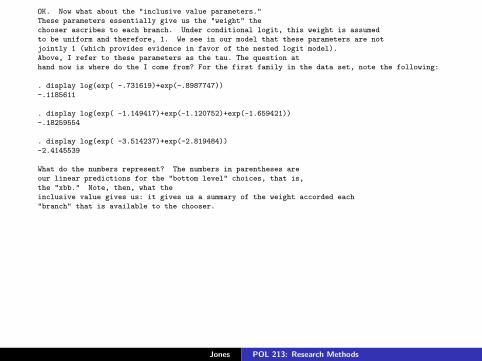
OK. Now what about the "inclusive value parameters."

These parameters essentially give us the "weight" the

chooser ascribes to each branch. Under conditional logit, this weight is assumed

to be uniform and therefore, 1. We see in our model that these parameters are not

jointly 1 (which provides evidence in favor of the nested logit model).

Above, I refer to these parameters as the tau. The question at

hand now is where do the I come from? For the first family in the data set, note the following:

. display log(exp( -.731619)+exp(-.8987747))

-.1185611

. display log(exp( -1.149417)+exp(-1.120752)+exp(-1.659421))

-.18259554

. display log(exp( -3.514237)+exp(-2.819484))

-2.4145539

What do the numbers represent? The numbers in parentheses are

our linear predictions for the "bottom level" choices, that is,

the "xbb." Note, then, what the

inclusive value gives us: it gives us a summary of the weight accorded each

"branch" that is available to the chooser.


Ok, almost done. Now what about the top-level probabilities

(i.e. the probability of choosing fast food, family, or fancy?).

In lecture, I give the function. To compute it directly, we do the following:

. display exp(-1.191674 +_b[/fast]*-.1185611)/

(exp( -1.191674 + _b[/fast]*-.1185611) + exp(1.425016 +_b[/fancy]*-2.414554)

+ exp(0 +_b[/family]*-.1825957))

.15345345

Note where these numbers come from: they are the taus, the "ivb," and the "xb1."

In doing this exercise, we reproduce pb1. Interpretation?

The probability of choosing a fast food restaurant is .15 for a person

with this covariate profile.


Finally, we can compute the "bottom-level" probability.

It is the simple conditional probability result. For the first observation, it is:

. display p1*condpb

.08312449

We could then "fill in the tree" for observation 1 (if we wanted to).



I So what would we get from this model if we fully interpretedit?

I The probability of choice j . That is, the unconditionalprobability.

I The conditional probability of choice j given the selection ofbranch i .

I The probability of choosing branch i .

I A direct test of the weight associated with each branch, givenchooser attributes.

I Seems a useful empirical model for testing rational choicepredictions.

I Data requirements are substantial, as is theory for nestingchoices.


Nested Logit - University of California, Davispsfaculty.ucdavis.edu/bsjjones/nestedlogit.pdf · I...

Documents

Transcript of Nested Logit - University of California, Davispsfaculty.ucdavis.edu/bsjjones/nestedlogit.pdf · I...