Munich Personal RePEc Archive

Neoclassical Theory versus New

Economic Geography. Competing

explanations of cross-regional variation in

economic development

Fingleton, Bernard and Fischer, Manfred M.

University of Strathclyde, Scotland, UK, Vienna University of

Economics and Business

2010

Online at https://mpra.ub.uni-muenchen.de/77554/

MPRA Paper No. 77554, posted 03 Apr 2017 10:13 UTC

Neoclassical Theory versus New Economic Geography. Competing explanations of cross-regional variation in economic development

Bernard Fingleton

Department of Economics, University of Strathclyde

Scotland, UK

Manfred M. Fischer

Institute for Economic Geography and GIScience

Vienna University of Economics and BA, Vienna, Austria

Abstract. This paper uses data for 255 NUTS-2 European regions over the period 1995-2003

to test the relative explanatory performance of two important rival theories seeking to explain

variations in the level of economic development across regions, namely the neoclassical

model originating from the work of Solow (1956) and the so-called Wage Equation, which is

one of a set of simultaneous equations consistent with the short-run equilibrium of new

economic geography (NEG) theory, as described by Fujita, Krugman and Venables (1999).

The rivals are non-nested, so that testing is accomplished both by fitting the reduced form

models individually and by simply combining the two rivals to create a composite model in an

attempt to identify the dominant theory. We use different estimators for the resulting panel

data model to account variously for interregional heterogeneity, endogeneity, and temporal

and spatial dependence, including maximum likelihood with and without fixed effects, two

stage least squares and feasible generalised spatial two stage least squares plus GMM; also

most of these models embody a spatial autoregressive error process. These show that the

estimated NEG model parameters correspond to theoretical expectation, whereas the

parameter estimates derived from the neoclassical model reduced form are sometimes

insignificant or take on counterintuitive signs. This casts doubt on the appropriateness of

neoclassical theory as a basis for explaining cross-regional variation in economic

development in Europe, whereas NEG theory seems to hold in the face of competition from

its rival.

Keywords: New economic geography, augmented Solow model, panel data model, spatially

correlated error components, spatial econometrics

JEL Classification: C33, O10

1

1 Introduction

In recent years New Economic Geography (NEG) has rivalled neoclassical growth theory as a

way of explaining spatial variation in economic development. This new theory is particularly

appealing because increasing returns to scale are fundamental to a proper understanding of

spatial disparities in economic development, and several attempts have been made to

operationalise and test various versions of NEG theory with real world data (see for example

Fingleton 2005, 2007b). Much of this work focuses around the short-run equilibrium wage

equation (see Roos 2001, Davis and Weinstein 2003, Mion 2004, Redding and Venables

2004, Head and Mayer 2006), which – although only one of the several simultaneous

equations that define a complete NEG model – is probably the most important and easily

tested relationship coming from the theory.

In the spirit of Fingleton (2007a), this paper aims to test whether the success of the NEG

Wage Equation is replicated in data on European regions, under the challenge of the

competing neoclassical conditional convergence (NCC) model. This paper provides some new

evidence using, for the first time, data extending to the whole of the EU, including the new

accession countries. We control for country-specific heterogeneity relating to these new

accession countries throughout. Testing is accomplished by considering the rival models in

isolation followed by combining the two rival non-nested models within a composite spatial

panel data model, usually with a spatial error process to allow for omitted spatially correlated

variables or other unmodeled causes of spatial dependence. Unlike Fingleton (2007a), we

seek to include a price index in our measurement of market potential, which is the key

variable in the NEG model.

The paper is structured as follows. Section 2 introduces the two relevant theoretical models,

first, the neoclassical theory leading to the reduced form for the NCC model in Section 2.1,

and then the rival NEG model in Section 2.2, leading to the competing reduced form. Section

3 outlines the composite spatial panel data model in Section 3.1. Section 3.2 continues to

describe a procedure for estimating this nesting model. Section 4.1 describes the data, the

sample of regions and the construction of the market potential variable, while Section 4.2

presents the resulting estimates. Section 5 concludes the paper.

2 The theoretical models

2

2.1 Neoclassical theory and the reduced model form

Neoclassical growth models are characterised by three central assumptions. First, the level of

technology is considered as given and thus exogenously determined, second the production

function shows constant returns to scale in the production factors for a given, constant level of

technology. Third, the production factors have diminishing marginal products. This

assumption of diminishing returns is central to neoclassical growth theory.

The theory used in this paper is based on a variation of Solow’s (1956) growth model that

contains elements of models by Mankiw, Romer and Weil (1992), and Jones (1997). We

suppose that output Y in a regional economy i=1, …, N at time t=1, …, T is produced by

combining physical capital K with skilled labour H according to a constant-returns-to-scale

Cobb-Douglas production function

1( , ) ( , ) [ ( , ) ( , )]Y i t K i t A i t H i t

α α−= (1)

where A is the labour-augmenting technological (total factor productivity) shift parameter so

that ( , ) ( , )A i t H i t may be thought of as the supply of efficiency units of labour in region i at

time t. The exponents ,α 0 1α< < , and (1 )α− are the output elasticities of physical capital

and effective labour, respectively. Skilled labour input is given1 by

( , ) ( , ) ( , )H i t h i t L i t= (2)

where L is raw labour input in region i, and h some region-specific measure of labour

efficiency. Raw labour L and technology A are assumed to grow exogenously at rates n and

g . While technology growth g is supposed to be uniform in all regions2, the growth of labour

may differ from region to region. Thus, the number of effective units of labour, ( , ) ( , )A i t H i t ,

grows at rate ( , )n i t g+ .

Letting lowercase letters denote variables normalised by the size of effective labour force,

then the regional production function may be rewritten in its intensive form as

( , ) ( ) ( , )y i t f k k i tα≡ = (3)

1 Note that this way of modelling skilled labour guarantees constant returns to scale. The implication that factor

payments exhaust output is preserved by assuming that the human capital is embodied in labour (Jones 1997).

2 At some level this assumption appears to be reasonable. For example, if technological progress is viewed to be

the engine of growth, one might expect that technology transfer across space will keep regions away from

diverging infinitely, and one way of interpreting this statement is that growth rates of technology will

ultimately be the same across regions (Jones 1997). Note that we do not require the levels of technology to be

the same across regions.

3

where y and k are regional output and capital per unit of effective labour, that is,

( , ) ( , ) / [ ( , ) ( , )]y i t Y i t A i t H i t= and ( , ) ( , ) / [ ( , ) ( , )]k i t K i t A i t H i t= .

We can then examine how output reacts to an increase in capital, that is, we look at the

derivatives of output y with respect to k. Then

1

0'( ) ( , ) 0, lim[ '( )] 0 lim[ '( )]

k kf k k i t f k and f k

αα −

→∞ →= > = = ∞ (4a)

2''( ) (1 ) , ''( ) 0.f k k f kαα α −= − − < (4b)

From Eqs. (4a) and (4b) we see that the first derivative is positive, but declines as capital goes

to infinity, and becomes very large if the amount of capital is infinitely small, features known

as Inada condition. This means that the marginal product of capital is positive, but it declines

with rising capital. Thus, all other factors equal, any additional amount of physical capital will

yield a decreasing rate of return in the production function. This assumption is central to the

neoclassical model of growth. Under this assumption capital accumulation does not make a

constant contribution to income growth. While accumulating capital, an additional unit of

capital makes a smaller contribution to output than the previous additional unit3.

The neoclassical model of growth postulates that a regional economy starting from a low level

of capital and low per effective worker income, accumulates capital and runs through a

growth process, where growth rates are initially higher, then decline, and finally approach

zero when the steady state per effective labour income is reached. The model predicts

conditional convergence in the sense that a lower value of income per effective labour unit

tends to generate a higher per effective labour growth rate, once we control for the

determinants of the steady state. The transition growth path of the single regional economy

can be transposed to the situation of N regional economies, which start from different levels.

If regional economies have the same steady state, the same transition dynamics will apply for

the whole cross-section of regions. Much of the cross-region difference in income per labour

force can be traced to differing determinants of the steady state in the neoclassical growth

model: population growth and accumulation of the physical capital.

3 Note that the assumption of diminishing returns has been challenged by new growth theory, which assumes

that constant or increasing returns can be an outcome of, for example, human capital accumulation or

knowledge spillovers.

4

Physical capital per effective labour in region i evolves according to

( , ) ( , ) ( , ) [ ( , ) ] ( , )Kk i t s i t y i t n i t g k i tδ•

= − + + (5)

where Ks is the investment rate4, n the rate of population growth, g and δ constant rates of

technology growth and capital depreciation, respectively. The dot over k denotes

differentiation with respect to time5.

This differential equation is the fundamental equation of the growth model. It indicates how

the rate of change of the regional capital stock at any point in time is determined by the

amount of capital already in existence at that date. Together with this historically given stock

of physical capital, Eq. (5) determines the entire path of capital. In order to maintain a fixed

capital stock per effective labour unit, the region must invest an amount to replace the

depreciated capital, ( , )k i tδ , and an amount to balance the growth of effective labour,

( , ) .n i t g+

Due to the diminishing marginal product of capital, per effective labour output available for

investment will become smaller with additional capital. Thus, investment per effective labour

is non-linear. It decreases with rising capital accumulation. Initially, investment exceeds the

term [ ( , ) ] ( , ),n i t g k i tδ+ + and hence the capital share per effective labour increases. As the

capital share goes to infinity, investment becomes less than the term [ ( , ) ] ( , ).n i t g k i tδ+ +

Thus, there is a point k∗ where investment is just sufficient to balance the second term on the

right hand side of Eq. (5). At k∗ the amount of capital per effective labour unit is constant,

( , ) 0.k i t•

= Thus, the steady state is given by the condition

( , ) ( , ) [ ( , ) ] ( , ).Ks i t k i t n i t g k i tα δ∗ ∗= + + (6)

It is then straightforward to solve for the value k∗

1

1

( , )( , )

( , )

Ks i tk i t

n i t g

α

δ

−

∗ ⎡ ⎤= ⎢ ⎥+ +⎣ ⎦

. (7)

4 The economy is closed so that saving equals investment, and the only use of investment in this economy is to

accumulate physical capital. The assumption that investment equals saving may seem too simple, the more if

we consider open regional economies. But, as Feldstein and Horioka (1980) have shown, the coincidence of

investments and savings is empirically valid across a set of regions, including open regions.

5 Note that the term on the left hand side of Eq. (5) is the continuous version of k(i, t)–k(i, t–1), that is the

change in the physical capital stock in efficient labour unit terms per time period.

5

Substituting Eq. (7) into the regional production function given by Eq. (3), and taking logs,

we find that steady state income per labour is

1 1

( , )ln ln ( , ) ln[ ( , ) ] ln ( , ) ln ( , )

( , )

Y i ts i t n i t g A i t h i t

L i t

α αα α δ− −= − + + + + . (8)

Of course, neither A nor h are observed directly, but may be modelled as a loglinear

relationship so that

1 2ln ( , ) ln ( , ) constant ln ( , ) ( , )A i t h i t S i t t i tβ β ξ+ = + + + (9)

where the level of regional technology, ( , )A i t , is proxied by a deterministic trend, and the

region- and time-specific measure of labour efficiency, ( , ),h i t by the skills ( , )S i t of the

workforce as given by the level of educational attainment of the population. The rationale for

this proxy is the widely recognised link between labour efficiency and schooling. ( , )i tξ is an

iid disturbance term with zero mean and constant variance, and 1β and 2β are scalar

parameters.

Substituting Eq. (9) into Eq. (8) yields the following estimation equation:

1 21

( , )ln constant ln[ '( , ) ln ( , )] ln ( , ) ( , )

( , )

Y i tn i t s i t S i t t i t

L i t

αα β β ε−= − − + + + (10)

with '( , ) ( , )n i t n i t g δ= + + and ln '( , ) ln ( , )n i t s i t− referred to as the log-adjusted population

growth rate.

Most recently, Koch(2008) has formally extended the neoclassical model in order to capture

spillover effects. To save space we do not replicate his extended model structure in the current

paper, although account is taken of spatial effects in subsequent modelling.

2.2 NEG theory and the reduced model form

Whereas in the neoclassical model output per worker follows the long-run equilibrium path,

in the NEG framework we view output per worker [or equivalently nominal wages] as a short-

6

run equilibrium6 phenomenon. Only in the very long-run – which we do not consider here –

does factor mobility eliminate real wage differences.

The NEG theory used here is that set out by Fujita, Krugman and Venables (1999) which has

as a basis the Dixit-Stiglitz model of monopolistic competition (Dixit and Stiglitz 1977), with

two sectors, N regions and transportation costs between these regions. Important components

of the model are the elasticity of substitution ( )σ between product varieties, and

transportation costs of monopolistic competition goods from region i to region j.

Transportation costs – in terms of Samuelson’s iceberg form – are a basic element of the NEG

theory advanced by Fujita, Krugman and Venables (1999) since they determine the

attractiveness of production locations in terms of access to markets.

The traditional full general equilibrium model comprises two sectors: a perfectly competitive

sector (called C-sector) that produces a single, homogeneous good under constant returns to

scale, whereas the other sector, termed the M-sector, exhibits a monopolistically competitive

market structure and a large variety of differentiated goods. The production of each M variety

exhibits internal increasing returns to scale.

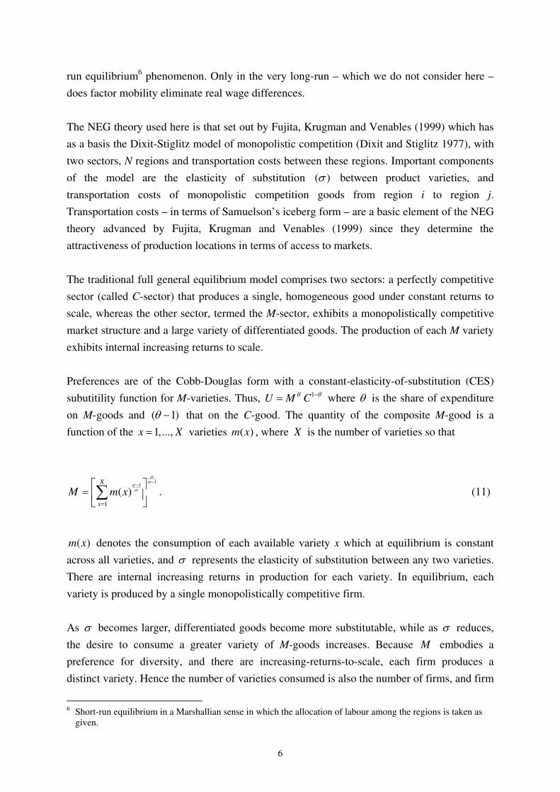
Preferences are of the Cobb-Douglas form with a constant-elasticity-of-substitution (CES)

subutitility function for M-varieties. Thus, 1U M C

θ θ−= where θ is the share of expenditure

on M-goods and ( 1)θ − that on the C-good. The quantity of the composite M-good is a

function of the 1,...,x X= varieties ( )m x , where X is the number of varieties so that

11

1

( )X

x

M m x

σσ

σσ

−−

=

⎡ ⎤= ⎢ ⎥⎣ ⎦∑ . (11)

( )m x denotes the consumption of each available variety x which at equilibrium is constant

across all varieties, and σ represents the elasticity of substitution between any two varieties.

There are internal increasing returns in production for each variety. In equilibrium, each

variety is produced by a single monopolistically competitive firm.

As σ becomes larger, differentiated goods become more substitutable, while as σ reduces,

the desire to consume a greater variety of M-goods increases. Because M embodies a

preference for diversity, and there are increasing-returns-to-scale, each firm produces a

distinct variety. Hence the number of varieties consumed is also the number of firms, and firm

6 Short-run equilibrium in a Marshallian sense in which the allocation of labour among the regions is taken as

given.

7

output equals demand for that variety. Choosing units of measurement in a way that shifts

attention from the number of firms and product prices to the number of workers and their

wage rates, Fujita, Krugman and Venables (1999, Chapter 4) introduce simplifying

normalizations so that θ is also equal to the equilibrium number of workers per firm and to

the equilibrium output per firm.

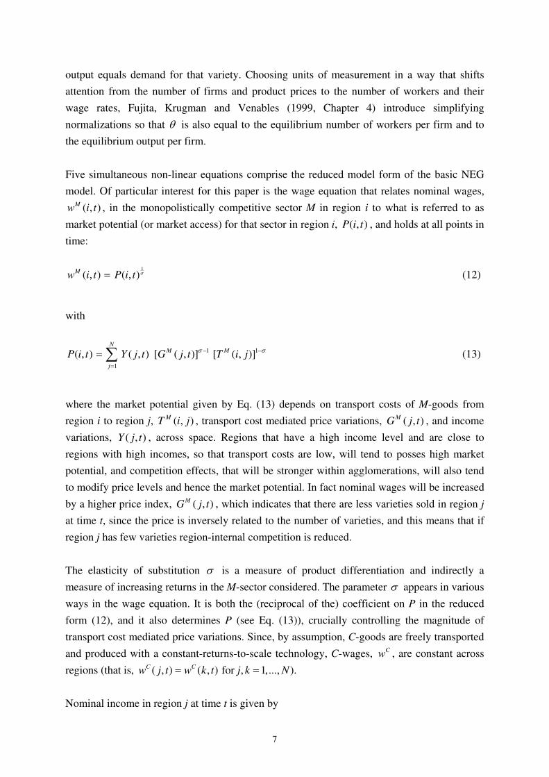
Five simultaneous non-linear equations comprise the reduced model form of the basic NEG

model. Of particular interest for this paper is the wage equation that relates nominal wages,

( , )Mw i t , in the monopolistically competitive sector M in region i to what is referred to as

market potential (or market access) for that sector in region i, ( , )P i t , and holds at all points in

time:

1

( , ) ( , )Mw i t P i t σ= (12)

with

1 1

1

( , ) ( , ) [ ( , )] [ ( , )]N

M M

j

P i t Y j t G j t T i jσ σ− −

=

= ∑ (13)

where the market potential given by Eq. (13) depends on transport costs of M-goods from

region i to region j, ( , )MT i j , transport cost mediated price variations, ( , )M

G j t , and income

variations, ( , )Y j t , across space. Regions that have a high income level and are close to

regions with high incomes, so that transport costs are low, will tend to posses high market

potential, and competition effects, that will be stronger within agglomerations, will also tend

to modify price levels and hence the market potential. In fact nominal wages will be increased

by a higher price index, ( , )MG j t , which indicates that there are less varieties sold in region j

at time t, since the price is inversely related to the number of varieties, and this means that if

region j has few varieties region-internal competition is reduced.

The elasticity of substitution σ is a measure of product differentiation and indirectly a

measure of increasing returns in the M-sector considered. The parameter σ appears in various

ways in the wage equation. It is both the (reciprocal of the) coefficient on P in the reduced

form (12), and it also determines P (see Eq. (13)), crucially controlling the magnitude of

transport cost mediated price variations. Since, by assumption, C-goods are freely transported

and produced with a constant-returns-to-scale technology, C-wages, Cw , are constant across

regions (that is, ( , ) ( , ) for , 1,..., ).C Cw j t w k t j k N= =

Nominal income in region j at time t is given by

8

( , ) ( , ) ( , ) (1 ) ( , ) ( , )M CY j t j t w j t j t w j tθ λ θ φ= + − (14)

where θ is the expenditure share of M-goods, λ and φ are the shares of total supply of M-

and C-workers in region j, while Cw is the wage rate of workers in the competitive sector in j

at time t.

The M-price index ( , )MG j t for region j at time t is

1

1

1

1

( , ) ( , ) [ ( , ) ( , )]N

M M M

k

G j t k t w k t T k jσ

σλ−

−

=

⎧ ⎫= ⎨ ⎬⎩ ⎭∑ (15)

where the number of varieties produced in region k is represented by ( , )k tλ which is equal to

the share in region k of the total supply of M-workers in region k.

We follow Fujita, Krugman and Venables (1999) in calling Eq. (12) the NEG-Wage Equation

that represents a short-run equilibrium relationship based on the assumption that factor

mobility in response to real wage differences in the monopolistic competition sector is slow

compared with the instantaneous entry and exit of M-firms so that profits are immediately

driven to zero. It is only in the very long-run that we would expect movement to a stable long-

run equilibrium resulting from labour migration.

This wage equation is an exceptionally simple relationship. To add an extra injection of

realism we assume that wages, w(i, t), also depend on the efficiency level of the labour force,

( , ),h i t so that

1

( , ) ( , ) ( , )w i t P i t h i tσ= . (16)

Taking logs and assuming that ( , )h i t may be proxied by ( , )S i t yields the extended NEG-

Wage Equation

0 1 2

1ln ( , ) ln ( , ) ln ( , ) ( , )w i t P i t S i t t i tβ β β η

σ= + + + + (17)

where η is independently and identically distributed with zero mean and constant variance.

This equation is the counterpart to Eq. (10), but has a fundamentally different theoretical

provenience, and has somewhat different long-run implications. Note that the deterministic

time trend t is also introduced as an extra regressor, in order to control for the evolution of the

9

level of regional technology. Otherwise this may be picked up by P and the significance of P

may be largely attributable to this rather than to true NEG processes.

3 Testing the non-nested rival models

Assessing the relative explanatory performance of the NEG-Wage Equation (17) and the

neoclassical model (10) is accomplished by setting up a composite spatial panel data model

within which both models are nested. The rival models are not special cases of each other, but

special cases of the data generating process (DGP) of the regressors in the composite model.

The problem of deciding between the competing models then amounts to considering whether

any one rival encompasses the DGP. By encompassing we mean that one model can explain

the results of another (Fingleton 2006).

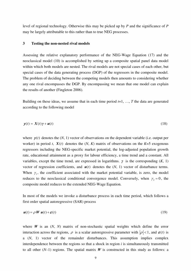
Building on these ideas, we assume that in each time period t=1, …, T the data are generated

according to the following model

( ) ( ) ( )t t t= +y X γ u (18)

where ( )ty denotes the (N, 1) vector of observations on the dependent variable (i.e. output per

worker) in period t, ( )tX denotes the (N, K) matrix of observations on the K=5 exogenous

regressors including the NEG-specific market potential, the log-adjusted population growth

rate, educational attainment as a proxy for labour efficiency, a time trend and a constant. All

variables, except the time trend, are expressed in logarithms. γ is the corresponding (K, 1)

vector of regression coefficients, and ( )tu denotes the (N, 1) vector of disturbance terms.

When 1γ , the coefficient associated with the market potential variable, is zero, the model

reduces to the neoclassical conditional convergence model. Conversely, when 2 0γ = , the

composite model reduces to the extended NEG-Wage Equation.

In most of the models we invoke a disturbance process in each time period, which follows a

first order spatial autoregressive (SAR) process

( ) ( ) ( )t t tρ= +u W u ε (19)

where W is an (N, N) matrix of non-stochastic spatial weights which define the error

interaction across the regions, ρ is a scalar autoregressive parameter with 1ρ < , and ( )tε is

a (N, 1) vector of the remainder disturbances. This assumption implies complex

interdependence between the regions so that a shock in region i is simultaneously transmitted

to all other (N–1) regions. The spatial matrix W is constructed in this study as follows: a

10

neighbouring region takes the value one, otherwise it is zero. The rows of this matrix are

normalised so that they sum to one.

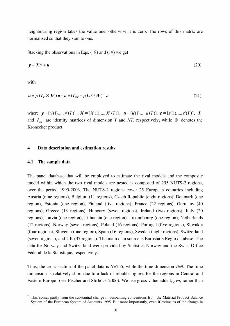
Stacking the observations in Eqs. (18) and (19) we get

= +y X γ u (20)

with

1( ) ( )T NT Tρ ρ −= ⊗ + = − ⊗u I W u I I Wε ε (21)

where [ '(1),..., ' ( )]' , [ '(1),..., ' ( )]',y y T X X T=y X = [ '(1),..., '( )]', [ '(1),..., '( )]',u u T Tε ε=u =ε TI

and NTI are identity matrices of dimension T and NT, respectively, while ⊗ denotes the

Kronecker product.

4 Data description and estimation results

4.1 The sample data

The panel database that will be employed to estimate the rival models and the composite

model within which the two rival models are nested is composed of 255 NUTS-2 regions,

over the period 1995-2003. The NUTS-2 regions cover 25 European countries including

Austria (nine regions), Belgium (11 regions), Czech Republic (eight regions), Denmark (one

region), Estonia (one region), Finland (five regions), France (22 regions), Germany (40

regions), Greece (13 regions), Hungary (seven regions), Ireland (two regions), Italy (20

regions), Latvia (one region), Lithuania (one region), Luxembourg (one region), Netherlands

(12 regions), Norway (seven regions), Poland (16 regions), Portugal (five regions), Slovakia

(four regions), Slovenia (one region), Spain (16 regions), Sweden (eight regions), Switzerland

(seven regions), and UK (37 regions). The main data source is Eurostat’s Regio database. The

data for Norway and Switzerland were provided by Statistics Norway and the Swiss Office

Féderal de la Statistique, respectively.

Thus, the cross-section of the panel data is N=255, while the time dimension T=9. The time

dimension is relatively short due to a lack of reliable figures for the regions in Central and

Eastern Europe7 (see Fischer and Stirböck 2006). We use gross value added, gva, rather than

7 This comes partly from the substantial change in accounting conventions from the Material Product Balance

System of the European System of Accounts 1995. But more importantly, even if estimates of the change in

11

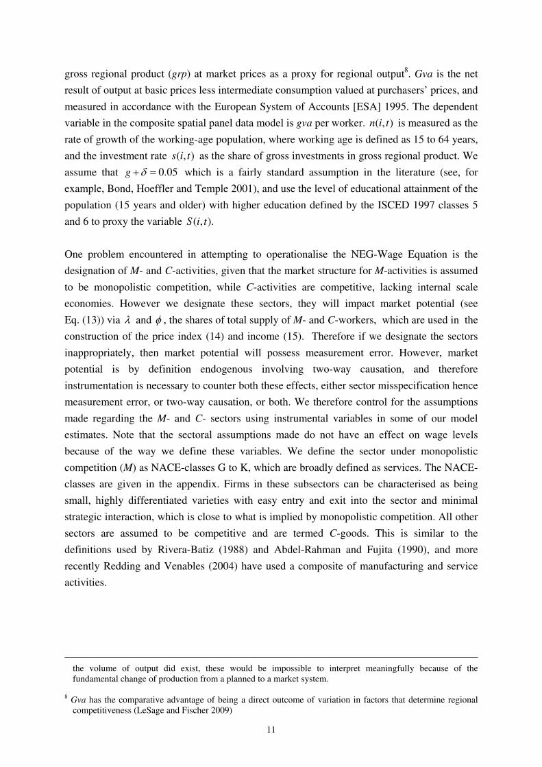
gross regional product (grp) at market prices as a proxy for regional output8. Gva is the net

result of output at basic prices less intermediate consumption valued at purchasers’ prices, and

measured in accordance with the European System of Accounts [ESA] 1995. The dependent

variable in the composite spatial panel data model is gva per worker. ( , )n i t is measured as the

rate of growth of the working-age population, where working age is defined as 15 to 64 years,

and the investment rate ( , )s i t as the share of gross investments in gross regional product. We

assume that 0.05g δ+ = which is a fairly standard assumption in the literature (see, for

example, Bond, Hoeffler and Temple 2001), and use the level of educational attainment of the

population (15 years and older) with higher education defined by the ISCED 1997 classes 5

and 6 to proxy the variable ( , ).S i t

One problem encountered in attempting to operationalise the NEG-Wage Equation is the

designation of M- and C-activities, given that the market structure for M-activities is assumed

to be monopolistic competition, while C-activities are competitive, lacking internal scale

economies. However we designate these sectors, they will impact market potential (see

Eq. (13)) via λ and φ , the shares of total supply of M- and C-workers, which are used in the

construction of the price index (14) and income (15). Therefore if we designate the sectors

inappropriately, then market potential will possess measurement error. However, market

potential is by definition endogenous involving two-way causation, and therefore

instrumentation is necessary to counter both these effects, either sector misspecification hence

measurement error, or two-way causation, or both. We therefore control for the assumptions

made regarding the M- and C- sectors using instrumental variables in some of our model

estimates. Note that the sectoral assumptions made do not have an effect on wage levels

because of the way we define these variables. We define the sector under monopolistic

competition (M) as NACE-classes G to K, which are broadly defined as services. The NACE-

classes are given in the appendix. Firms in these subsectors can be characterised as being

small, highly differentiated varieties with easy entry and exit into the sector and minimal

strategic interaction, which is close to what is implied by monopolistic competition. All other

sectors are assumed to be competitive and are termed C-goods. This is similar to the

definitions used by Rivera-Batiz (1988) and Abdel-Rahman and Fujita (1990), and more

recently Redding and Venables (2004) have used a composite of manufacturing and service

activities.

the volume of output did exist, these would be impossible to interpret meaningfully because of the

fundamental change of production from a planned to a market system.

8 Gva has the comparative advantage of being a direct outcome of variation in factors that determine regional

competitiveness (LeSage and Fischer 2009)

12

Given these definitions, it is possible to measure the market potential variable ( , )P i t defined

by Eq. (13). In order to quantify the variable, we have assumed that the parameter9 σ is equal

to 6.5, and calculated income, M-prices and transportation costs. Income is defined by

Eq. (14), and depends on the assumed M- and C-sector wage rates ( Mw gva= per M-worker,

Cw mean gva= per C-worker, averaging across all 255 regions

10), the share λ of the M-

sector and the share φ of the C-sector employment in each region, the share θ of the

European (total 255 NUTS-2 regions) workforce that is employed in the monopolistic

competition sector M, and the share (1 )θ− of the total European workforce that is employed

in the competitive sector C .

M-prices are defined by Eq. (15), and these are quantified using again the M-employment

shares λ in each region, the assumed M-wage rate (equal to gva per M-worker) for each

region, and the transport costs from each region. We assume iceberg transport costs11

of the

form

23

exp[ ln ( , )] for

( , ) ( )for

ij

M

d i j d i j

T i j R ii j

ττ

π

⎧ = ≠⎪= ⎨

=⎪⎩

(22)

with an area-based approximation of intra-regional distances. ( )R i is region’s i area measured

in terms of square km, and ( , )d i j denotes the great circle distance from region i to region j,

represented by their economic centres. The use of the natural logarithm of distance rather than

distance per se implies a power functional relationship between transport costs and distance.

For the (exogenous) distance multiplier τ we adopt the value 2τ = throughout the analysis12

.

It is important to note that the iceberg transport cost function (22) maintains the constant

9 There is no theoretical a priori basis for choosing 6.5,σ = other than we expect the elasticity of substitution

1σ > under a monopolistic competition assumption (since /( 1)σ μ μ= − where 1μ > is the measure of

monopoly power, equal to one in the case of perfect competition). In fact, we use post hoc rationalisation to

justify this choice, since our preferred model estimates (see Table 2) imply a value not significantly different

from 6.5.

10 The rationale for this is that ( , )

Mw i t is the nominal wage rate in sector M and region i, which we approximate

by overall gva per worker. This undoubtedly leads to some measurement error which will be accommodated

by the model’s error term and by the use of instrumental variables for our market potential variable. In case of

( , )C

w i t , this is constant across regions, and is approximated by the mean.

11 “Iceberg transport costs” imply that only a fraction of the shipped good reaches its destination.

12 Ideally, the parameter τ should be obtained from trade data, but these are not available at the NUTS-2 level.

We assume 2τ = which implies that there are no economies of scale in distance transportation ( 1).τ ≥ This

is a strong assumption that has been seen as somewhat unrealistic (McCann 2005, McCann and Fingleton

2007), and we could choose 0 1τ≤ ≤ although opting for 2τ = does not diminish the relative performance

of the model which is the main focus of the paper.

13

elasticity of demand assumption that runs through the microeconomic theory underpinning the

NEG-Wage Equation.

4.2 Empirical results

The tables below show various panel regression estimates of the neoclassical growth model,

the rival NEG model, and the artificial nesting model which combines the variables from the

two theories under comparison. For each set of estimates, the dependent variable is the log of

gva per worker.

The neoclassical growth model

Table 1 presents the parameter estimates of the neoclassical growth model (10) using different

estimation procedures. The explanatory variables are the log-adjusted population growth rate

ln '( , ) ln ( , )n i t s i t− , log of share of residents with higher education (ln ( , ))S i t , the time trend

(1 to 9 for each of the years 1995 to 2003 inclusive), and dummy variables for each of the

new entrant countries (Poland, Hungary, Czech Republic, Slovakia, Slovenia, Estonia,

Lithuania and Latvia). Given that the growth rate of the working age population ( ')n and the

share of investment in gross regional product ( )s are lagged by one year, the adjusted log

population growth rate ln '( , ) ln ( , )n i t s i t− is treated as an exogenous variable13

. Since we are

setting the neoclassical model as the default model in this analysis, this is not an unreasonable

assumption since it means we avoid rejecting the default model too easily simply on account

of weak instruments. Following Mankiw, Romer and Weil (1992), we also relax the constraint

that the coefficients on ln '( , )n i t and ln ( , )s i t are equal in magnitude and opposite in sign,

leading to the unconstrained estimates given in the table (see columns 2, 4, 6 and 8).

Throughout, the variable ln ( , )S i t is assumed to be dependent principally on background

policy and social variables rather than on contemporaneous gva per worker levels.

Table 1 about here

The pooled OLS estimates (Table 1, column 1) show that the adjusted log population growth

rate is significantly positively related to the dependent variable, and we also see an increasing

share of residents with higher education [ln ( , )]S i t associated with a higher level of gva per

13 Note that for Halle, actual population growth for 1994-1995 means that '( , )n i t is negative for t = 1995 so that

we cannot calculate ln 'n . To remedy this, population growth is set to the 1995-1996 rate of -0.0078

14

worker. In addition there is a significant positive time trend effect, with gva per worker

increasing with time, reflecting an autonomously increasing level of technology. The country

dummy effects are all significantly negative, indicating that log gva per worker is

significantly reduced in the new entrant countries, by varying amounts, evidently due to

various institutional and structural differences, compared with the pre-2005 EU countries.

The ML estimates (Table 1, column 3) allow an autoregressive error process (Elhorst 2003;

Baltagi 2001) based on a 255 by 255 W matrix of ones and zeros, according to whether or not

a pair of regions is contiguous14

. This is standardised so that rows sum to one (and used

throughout). Although overall we see quite similar estimates to those from OLS estimation

(see column 3 in comparison to column 1), the presence of the highly significant

autoregressive parameter produces a similarly signed but smaller elasticity for

ln '( , ) ln ( , )n i t s i t− . In addition, the FGS2SLS estimates (Kapoor, Kelejian and Prucha 2007;

Fingleton 2007a, 2008) are quite similar to the ML estimates (see column 5 in comparison to

column 3). Fingleton (2007a) uses FGS2SLS for estimating the spatial panel data model

extending15

the generalised moments procedure suggested in Kapoor, Kelejian and Prucha

(2007) to the case of endogenous right-hand-side variables, such as the market potential. In

this case the variables are used as instruments for themselves, in other words we initially

assume exogeneity. On the other hand, controlling for spatial heterogeneity via region-

specific fixed effects eradicates the significance of ln '( , ) ln ( , )n i t s i t− and ln ( , )S i t . The very

high level of fit for this fixed effect panel data model reflects the impact of the unobserved

region-specific effects, the autoregressive process and the time trend. Given the presence of

these variables, ln '( , ) ln ( , )n i t s i t− and ln ( , )S i t carry no additional explanatory information.

In particular the region-specific effects represent catch-alls probably for a range of factors,

including ln '( , ) ln ( , )n i t s i t− and ln ( , )S i t . This casts some doubt on the real significance of

these two variables, which could be simply picking up the effect of some of these factors

when the fixed effects are omitted.

Table 1 also gives estimates without the restriction on the coefficients on ln '( , )n i t and

ln ( , )s i t (see columns 2, 4, 6 and 8). The principal feature of these estimates is the

counterintuitive signs on these two separate variables. With regard to ln '( , )n i t , one would

expect a negative sign (compare Mankiw, Romer and Weil 1992), and anticipate a positive

sign for ln ( , )s i t . Instead, we see ln gva per worker increasing as ‘population’ growth

increases, and regions with high levels of the log of the investment to grp ratio (ln ( , ))s i t are

associated with low levels of ln gva per worker. This casts doubt on the neoclassical model as

an appropriate model for the EU regions.

14 For nine isolated regions it has been necessary to create artificial, contiguous neighbours.

15

The method initially developed by Kapoor, Kelejian and Prucha (2007) was in the context of exogenous

regressors, but is it quite straightforward to extend this in order to allow for endogeneity.

15

The results of fitting additional spatial effects (following Koch 2008), are essentially the

same. To capture spatial effects, we introduce the spatial lag of the dependent variable (WY)16

and spatially lagged exogenous right hand side variables (excluding the time trend and

country dummies), together with a spatial autoregressive error process, and fit the model by

the FGS2SLS and GMM procedure of Kapoor, Kelejian and Prucha (2007). The estimates

(and t ratios), ignoring the exogenous spatial lags and country dummies and focussing on the

unrestricted estimates, are Constant=1.2423 (2.3813) WY = 0.8624 (17.2512) ln '( , )n i t =

0.0450 (0.7719) ln ( , )s i t = -0.0691 (-1.4929) ln ( , )S i t =0.2803 (8.2503) and time trend

=0.0061 (2.8197). In this case the presence of WY leads to a negative estimate for the

autoregressive process parameter ρ = -0.1131, 2

νσ =0.0025, 2

1σ = 0.2101 and the Pearson

product moment correlation between fitted and actual values is equal to 0.97.

The NEG-Wage Equation

Table 2 summarises various estimates of the rival NEG model (17), and these are seen to be

more consistent with theoretical expectation and reasonably robust to model specification and

method of estimation. The dependent variable is the log of gva per worker and the

explanatory variables are ln P, ln S, the time trend, and the eight new entrant dummies.

Because the market potential variable ln P is endogenous, we employ two sets of instruments.

Instrument set I includes the natural log of the area of each of the 255 regions (in square km),

denoted by ln (sqkm), together with its spatial lag W ln (sqkm). Instrument set II includes the

variable denoted 3-groups, which has values equal to –1, 0, or 1 according to whether the

value of ln P is in the bottom third, middle or top third of the market values. Because this last

variable is based on the endogenous variable, it is in theory also correlated with the error

term, although it has nevertheless been suggested as a remedy for endogeneity (as discussed

in Kennedy, 2003), albeit due to measurement error.

The 2SLS estimates (see the first two columns in Table 2) show a significant positive

elasticity for the market potential regardless of the instruments adopted, although there is

some variation in magnitude. The Sargan test supports the assumption that the instruments are

independent of the errors, but the 2SLS estimates fail to account for significant residual

autocorrelation. In contrast, the ML estimates (see columns 3 and 4) allow residual

dependence modelled by a spatial autoregressive process, without allowing for the

endogeneity of the market potential variable ln ( , ).P i t Nevertheless, it is noteworthy that even

in the presence of the region-specific fixed effects, ln ( , )P i t retains its significance and is

appropriately signed.

16 Since the spatial lag of the dependent variable is endogenous, this variable is instrumented by a variable coded

1, 0 or -1 according to whether the spatial lag of the log of gva per worker is in the top third, middle third, or

lower third of values, as discussed in Fingleton and Le Gallo (2008).

16

Table 2 about here

Columns 5 and 6 summarise NEG models accounting for both residual dependence and

endogeneity, estimated via FGS2SLS using the two different sets of instruments. For

comparison, the final column of Table 2 also gives estimates based on using ln ( , )P i t as an

instrument for itself. The estimates based on Instrument set I are the preferred ones, since the

95% confidence interval includes the value 0.15385=1/6.5 which was used at the outset to

calculate the market potential variable. Therefore, these estimates are consistent with

theoretical expectation and support the assumed elasticity of substitution which was used to

calculate ln ( , )P i t for 1,..., 255i = over the period 1995-2003.

The artificial nesting model

Our final appraisal of the two rival models comes from the parameter estimates of the

composite spatial panel data model (20)-(22), summarised in Table 3 and Table 4. Table 3

gives the ML estimates of the model for the restricted and the unrestricted cases with and

without region-specific fixed effects, and thus does not accommodate the endogeneity of the

market potential variable. The restricted models (see columns 1 and 2) reaffirm the earlier

results, with ln P retaining its significance while ln '( , ) ln ( , )n i t s i t− and ln ( , )S i t become

insignificant in the presence of region-specific fixed effects. The unrestricted models (see

columns 3 and 4) show counterintuitive signs on ln '( , )n i t and ln ( , ).s i t The unrestricted

model with fixed effects does not preserve the significance of the NCC variables.

Table 3 about here

Table 4 summarises models that allow for the endogeneity of the market potential variable.

The preferred estimates (based on Instruments I) retain the significance of ln '( , ) ln ( , )n i t s i t− ,

again suggesting that the neoclassical model is not encompassed by its rival (see column 1).

But in the unrestricted estimates (see columns 4-6) we again see that the NCC parameter signs

are counterintuitive, and also that ln '( , )n i t is insignificant. It thus appears that of the two

rival models, the NEG model is quite robust to methods of estimation and produces estimates

17

that appear to be reasonable a priori. The neoclassical growth model on the other hand fails in

the presence of fixed effects and in general produces parameter estimates that are contrary to

theoretical expectation and previous evidence.

Table 4 about here

Finally, we introduce the same additional spatial effects suggested by the Koch (2008) model

as was done for the neoclassical model, in other words we add spatially lagged endogenous

and exogenous variable to the model as described above, and use the same instruments as

outlined above. The outcome, focussing on the unrestricted model, is a set of FGS2SLS and

GMM estimates with signs conforming to the same pattern as indicated above but in which

the significance of the market potential variable is reduced. This, however, is none the less

sufficient for us to maintain our conclusion that the NEG model is dominant. Ignoring the

exogenous spatial lags and the country dummies, we find that the parameter estimates (and t

ratios) are as follows : Constant = 0.5829 (0.8670), WY = 0.8452 (16.4715), ln '( , )n i t =

0.04454 (0.7698), ln ( , )s i t = -0.0499 (-1.0634 ), ln ( , )S i t = 0.2652 (7.6604), ln ( , )P i t =

0.0908 (1.6846 ) and time trend = -0.0031 (-0.5068). In this case, a t-ratio of 1.6846 would

only be insignificant in a one-tailed test with test size equal to 0.05 if there were only 40

degrees of freedom, compared with the 2274 actually available. As with the neoclassical

version, the ANM model with extended spatial effects also gives a negative estimate for the

autoregressive process parameter ρ = -0.0880, 2

νσ = 0.0025, 2

1σ = 0.2100 and again the

Pearson product moment correlation between fitted and actual values is equal to 0.97.

5 Concluding remarks

We have shown that NEG theory provides a more plausible model of variations in wage levels

across 255 European regions than does the rival NCC model. This evidence is additional to

that given at the international scale in the companion paper by Fingleton(2008). While the

methodology in the two papers is similar, there are significant differences apart from data,

namely in the calculation of real market potential in the current paper, and the extension to

additional spatial effects following Koch (2008). It is evident from fitting the two reduced

forms separately, and jointly as an artifical nesting model, that the NCC model is

problematic17

. Our conclusion is based not solely on conventional statistical measures of

goodness of fit and methods for testing rival non-nested models, but also on the parameter

estimates obtained in relation to what we would anticipate from the competing theories. In

particular our estimated NEG Wage Equation invariably implies a significant positive

17 This interpretation is also an outcome of J test analyses which are not reported here for reasons of space.

18

coefficient 1σ > , which is what theory suggests. This remains true when confronting the

NEG-based Wage Equation with the NCC model in a composite spatial panel data model that

brings together both rival theories, and also when we estimate the individual models with

fixed effects which completely absorb interregional heterogeneity. In sharp contrast, the

coefficients derived from the reduced form of the NCC model take on counterintuitive signs

when the restrictions are removed, become insignificant or assume the wrong sign when

market potential is also present in the artificial nesting model. In addition, we also find that

when fixed effects are present, the NCC model parameters become insignificant, suggesting

that the theory-derived variables ln 'jt

n and lnjt

s may be simply capturing the effects of

omitted regressors that they correlate with.

Although these findings indicate that NEG theory is dominant, it too presents some

difficulties for estimation and has other serious limitations. One notable problem is the

endogeneity of the market potential variable, and this raises the problem of finding

appropriate instruments. In this case we feel our instruments satisfy the various requirements

of adequate instruments, although in general this type of modelling does require care in

instrument selection and testing. Moreover, while NEG theory is relatively superior to the

rival NCC theory in this particular case, it would seem that its applicability would depend on

the scale of analysis and that other competing theories may be superior in different contexts.

One significant problem with taking NEG theory too seriously is the inadequate way in which

transport costs are modelled, most conventionally via iceberg transport costs.

Our models are estimated using recent advances in the application of panel data techniques to

spatial data (see Baltagi 2005), where the issue of spatial dependence has led to some

innovatory approaches. In particular, we use a feasible generalised spatial two stage least

squares approach for estimating the spatial panel data model that extends the generalised

moments procedure suggested in Kapoor, Kelejian and Prucha (2007) to the case of

endogenous right-hand-side variables. We also employ ML estimation methods developed by

Elhorst (2003). The methodology is developing rapidly, and various other approaches have

been advocated in the literature which would also be interesting to pursue, such as moving

average error processes (Fingleton 2008) and modelling dependence using a factor error

structures (Pesaran 2007). One question that could be an issue with longer panel time series

would be whether or not the data possess unit roots. Baltagi et al. (2006) show that the size of

panel unit root tests will be biased under spatial error dependence, reflecting recent unit root

tests allowing for cross-sectional dependence (see Choi 2002; Chang 2002; Pesaran 2007;

Phillips and Sul 2003). In this particular application, this is not an issue because it would not

be possible to test for unit roots with such a short series, so we are simply assuming

stationarity.

19

Acknowledgements. The authors gratefully acknowledge the grant no. P19025-G11 provided by the Austrian

Science Fund (FWF). We are grateful for comments received from participants at the NARSC meeting at

Brooklyn, New York, USA.

References

Abdel-Rahman H and Fujita M (1990) Product variety, Marshallian externalities and city size,

Journal of Regional Science 30, 165-183

Baltagi B H (2005) Econometric analysis of panel data. Third edition. John Wiley, Chichester

Baltagi B H, Bresson G and Pirotte A (2006) Panel unit root tests and spatial dependence.

Center for Policy Research, Working Paper No. 88, Maxwell School of Citizenship and

Public Affairs, Syracuse University

Bond S R, Hoeffler A and Temple J (2001) GMM estimation of empirical growth models.

Centre for Economic Policy Research (CEPRS), Discussion Paper No. 3048

Chang Y (2002) Nonlinear IV panel unit root tests with cross-sectional dependency, Journal

of Econometrics 110, 261-292

Choi I (2002) Combination unit root tests for cross-sectionally correlated panels, in Corbae D,

Durlauf S N and Hansen B E (eds) Econometric Theory and Practice, pp. 311–333,

Cambridge: Cambridge University Press.

Davis D R and Weinstein D E (2003) Market access, economic geography and comparative

advantage: An empirical test, Journal of International Economics 59, 1-23

Dixit A K and Stiglitz J E (1977) Monopolistic competition and optimum product diversity,

American Economic Review 67(3), 297-308

Elhorst J P (2003) Specification and estimation of spatial data models, International Regional

Science Review 26, 244-268

Feldstein M and Horioka C (1980) Domestic saving and international capital flows, Economic

Journal 90(358), 314-329

Feenstra RC (1994) New product varieties and the measurement of international prices,

American Economic Review 84, 157-177

Fingleton B (2008) A generalized method of moments estimator for a spatial panel model

with an endogenous spatial lag and spatial moving average errors, Spatial Economic

Analysis 3, 27-44

20

Fingleton B (2007a) Competing models of global dynamics: Evidence from panel models

with spatially correlated error components. Forthcoming, Economic Modelling (available

online from 7 November 2007)

Fingleton B (2007b) New economic geography: Some preliminaries, in Fingleton B (ed) New

Directions in Economic Geography, pp 11-52. Edward Elgar, Cheltenham

Fingleton B (2006) The new economic geography versus urban economics: An evaluation

using local wage rates in Great Britain, Oxford Economic Papers 58, 501-530

Fingleton B (2005) Towards applied geographical economics: Modelling relative wage rates,

incomes and prices for the regions of Great Britain, Applied Economics 37, 2417-2428

Fingleton B and McCann P (2007) Sinking the iceberg? On the treatment of transport costs in

new economic geography, in Fingleton B (ed.) New directions in economic geography,

pp. 168-203. Edward Elgar, Cheltenham

Fingleton B, J Le Gallo (2008) "Estimating spatial models with endogenous variables, a

spatial lag and spatially dependent disturbances: Finite sample properties" Papers in

Regional Science 87, 319-339

Fischer M M and Stirböck C (2006) Pan-European regional income growth and club-

convergence, Annals of Regional Science 40(4), 693-721

Fujita M, Krugman P and Venables A J (1999) The spatial economy. Cities, regions, and

international trade. The MIT Press, Cambridge [MA] and London

Head K and Mayer T (2006) Regional wage and employment responses to market potential in

the EU, Regional Science and Urban Economics 36, 573-594

Head K and Ries J (2001) Increasing returns versus national product differentiation as an

explanation for the pattern of US-Canada trade, American Economic Review 91(4), 858-

876

Hendry D F (1995) Dynamic econometrics. Oxford University Press, Oxford

Jones C I (1997) Convergence revisited, Journal of Economic Growth 2, 131-153

Kapoor M, Kelejian H H and Prucha I R (2007) Panel data models with spatially correlated

error components, Journal of Econometrics 140, 97-130

Kelejian H H and Prucha I R (1999) A generalized moments estimator for the autoregressive

parameter in a spatial model, International Economic Review 40, 509-533

Kennedy P (2003) A Guide to Econometrics, Fifth edition. Blackwell, Oxford

Koch W. (2008) Development Accounting with Spatial Effects, Spatial Economic Analysis

3(3) (forthcoming)

21

LeSage J P and Fischer M M (2009) Spatial growth regressions: Model specification,

estimation and interpretation, Spatial Economic Analysis 4 (forthcoming)

Mankiw N E, Romer D and Weil D N (1992) A contribution to the empirics of economic

growth, Quarterly Journal of Economics 107(2), 407-437

McCann P (2005) Transport costs and new economic geography, Journal of Economic

Geography 6, 1-14

Mion G (2004) Spatial externalities and empirical analysis: The case of Italy, Journal of

Urban Economics 56, 97-118

Pesaran M H (2007) A simple panel unit root test in the presence of cross-sectional

dependence, Journal of Applied Econometrics 22, 265-312

Phillips P C B and Sul D (2003) Dynamic panel estimation and homogeneity testing under

cross-section dependence, Econometrics Journal 6, 217-259

Redding S and Venables A J (2004) Economic geography and international inequality,

Journal of International Economics 62, 53-82

Rivera-Batiz F (1988) Increasing returns, monopolistic competition, and agglomeration

economies in consumption and production, Regional Science and Urban Economics

18(1), 125-153

Roos M (2001) Wages and market potential in Germany, Jahrbuch für Regionalwissenschaft

21, 171-195

Solow R M (1956) A contribution to the theory of economic growth, Quarterly Journal of

Economics 70, 65-94

22

Appendix

TOTAL All NACE branches - Total

A_TO_P All NACE branches - Total (excluding extra-territorial organisations and bodies)

A_B Agriculture, hunting, forestry and fishing

A Agriculture, hunting and forestry

B Fishing

C_D_E Total industry (excluding construction)

C_TO_F Industry

C Mining and quarrying

D Manufacturing

E Electricity, gas and water supply

F Construction

G_TO_P Services (excluding extra-territorial organisations and bodies)

G_H_I Wholesale and retail trade, repair of motor vehicles, motorcycles and personal and

household goods; hotels and restaurants; transport, storage and communication

G Wholesale and retail trade; repair of motor vehicles, motorcycles and personal and

household goods

H Hotels and restaurants

I Transport, storage and communication

J_K Financial intermediation; real estate, renting and business activities

J Financial intermediation

K Real estate, renting and business activities

L_TO_P Public administration and defence, compulsory social security; education; health and

social work; other community, social and personal service activities; private

households with employed persons

L Public administration and defence; compulsory social security

M Education

N Health and social work

O Other community, social, personal service activities

P Activities of households

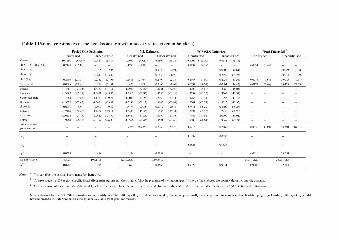
Table 1 Parameter estimates of the neoclassical growth model (t-ratios given in brackets)

Pooled OLS Estimates ML Estimates FGS2SLS Estimatesa Fixed Effects ML

b

Constrained Unconstrained Constrained Unconstrained Constrained Unconstrained Constrained Unconstrained

Constant 10.1390 (269.94) 9.6427 (88.89) 10.0667 (243.81) 9.8800 (118.35) 10.1061 (103.00) 9.8111 (51.18) -- -- -- --

ln '( , ) ln ( , )n i t s i t− 0.2141 (12.12) -- -- 0.1251 (8.79) -- -- 0.1737 (4.38) -- -- 0.0031 (0.46) -- --

ln '( , )n i t -- -- 0.0705 (2.05) -- -- 0.0722 (2.91) -- -- 0.0903 (1.64) -- -- 0.0029 (0.28)

ln ( , )s i t -- -- -0.2612 (-13.02) -- -- -0.1452 (-8.90) -- -- -0.2059 (-4.28) -- -- -0.0034 (-0.39)

ln ( , )S i t 0.2596 (21.94) 0.2583 (21.93) 0.2409 (23.64) 0.2404 (23.56) 0.2547 (7.60) 0.2535 (7.58) 0.0075 (0.61) 0.0075 (0.61)

Time trend 0.0388 (20.94) 0.0394 (21.31) 0.0401 (8.09) 0.0404 (8.04) 0.0397 (19.07) 0.0401 (19.42) 0.0472 (22.66) 0.0473 (22.43)

Poland -1.4468 (-71.34) -1.4633 (-71.51) -1.2989 (-42.35) -1.3081 (-42.03) -1.4227 (-15.86) -1.4365 (-16.03) -- -- -- --

Hungary -1.3293 (-45.39) -1.3490 (-45.86) -1.3515 (-31.95) -1.3593 (-31.89) -1.3638 (-11.23) -1.3762 (-11.39) -- -- -- --

Czech Republic -1.1384 (-39.67) -1.1351 (-39.74) -1.2037 (-41.23) -1.2030 (-41.11) -1.1768 (-13.14) -1.1755 (-13.15) -- -- -- --

Slovakia -1.3078 (-33.65) -1.3011 (-33.62) -1.3149 (-39.17) -1.3143 (-39.04) -1.3344 (-13.37) -1.3315 (-13.37) -- -- -- --

Slovenia 0.6990 (-9.33) -0.7003 (-9.39) -0.8774 (-20.35) -0.8772 (-20.34) -0.8314 (-6.29) -0.8309 (-6.27) -- -- -- --

Estonia -1.7169 (-22.68) -1.7456 (-23.11) -1.6433 (-17.57) -1.6506 (-17.51) -1.7291 (-7.15) -1.7450 (-7.26) -- -- -- --

Lithuania -2.0351 (-27.15) -2.0623 (-27.57) -1.8487 (-31.22) -1.8566 (-31.18) -1.9946 (-11.82) -2.0105 (-11.92) -- -- -- --

Latvia 1.9761 (-26.38) -2.0194 (-26.90) -1.8556 (-21.43) -1.8691 (-21.40) -1.9686 (-8.64) -1.9947 (-8.79) -- -- -- --

Autoregressive

parameter ρ -- -- -- -- 0.7779 (63.35) 0.7740 (62.25) 0.7213 -- 0.7162 -- 0.8330 (83.09) 0.8350 (84.01)

2

νσ -- -- -- -- 0.0037 0.0036 -- --

2

1σ -- -- -- -- 0.1524 0.1536 -- --

2σ 0.0501 0.0496 0.0184 0.0184 -- -- 0.0018 0.0018

Log likelihood 184.3020 196.1790 1,066.2639 1,069.3467 -- -- 3,687.6127 3,691.4583

R* c

0.8702 0.8715 0.8657 0.8666 0.9325 0.9331 0.9803 0.9803

Notes a The variables are used as instruments for themselves.

b To save space the 255 region-specific fixed effect estimates are not shown here. Also the presence of the region-specific fixed effects aliases the country dummies and the constant.

c R* is a measure of the overall fit of the model, defined as the correlation between the fitted and observed values of the dependent variable. In the case of OLS R* is equal to R-square.

Standard errors for the FGS2SLS estimates are not readily available, although they could be calculated by some computationally quite intensive procedures such as bootstrapping or jackknifing, although they would

not add much to the information we already have available from previous models.

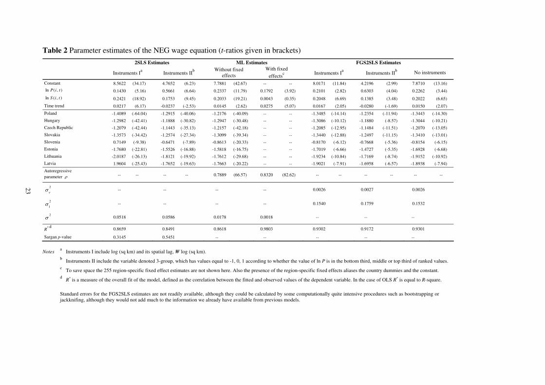
Table 2 Parameter estimates of the NEG wage equation (t-ratios given in brackets)

2SLS Estimates ML Estimates FGS2SLS Estimates

Instruments Ia Instruments II

b

Without fixed

effects

With fixed

effectsc

Instruments Ia Instruments II

b No instruments

Constant 8.5622 (34.17) 4.7652 (6.23) 7.7881 (42.67) -- -- 8.0171 (11.84) 4.2196 (2.99) 7.8710 (13.16)

ln ( , )P i t 0.1430 (5.16) 0.5661 (6.64) 0.2337 (11.79) 0.1792 (3.92) 0.2101 (2.82) 0.6303 (4.04) 0.2262 (3.44)

ln ( , )S i t 0.2421 (18.92) 0.1753 (9.45) 0.2033 (19.21) 0.0043 (0.35) 0.2048 (6.69) 0.1385 (3.48) 0.2022 (6.65)

Time trend 0.0217 (6.17) -0.0237 (-2.53) 0.0145 (2.62) 0.0275 (5.07) 0.0167 (2.05) -0.0280 (-1.69) 0.0150 (2.07)

Poland -1.4089 (-64.04) -1.2915 (-40.06) -1.2176 (-40.09) -- -- -1.3485 (-14.14) -1.2354 (-11.94) -1.3443 (-14.30)

Hungary -1.2982 (-42.41) -1.1888 (-30.82) -1.2947 (-30.48) -- -- -1.3086 (-10.12) -1.1880 (-8.57) -1.3044 (-10.21)

Czech Republic -1.2079 (-42.44) -1.1443 (-35.13) -1.2157 (-42.18) -- -- -1.2085 (-12.95) -1.1484 (-11.51) -1.2070 (-13.05)

Slovakia -1.3573 (-34.42) -1.2574 (-27.34) -1.3099 (-39.34) -- -- -1.3440 (-12.88) -1.2497 (-11.15) -1.3410 (-13.01)

Slovenia 0.7149 (-9.38) -0.6471 (-7.89) -0.8613 (-20.33) -- -- -0.8170 (-6.12) -0.7668 (-5.36) -0.8154 (-6.15)

Estonia -1.7680 (-22.81) -1.5526 (-16.88) -1.5818 (-16.75) -- -- -1.7019 (-6.66) -1.4727 (-5.35) -1.6928 (-6.68)

Lithuania -2.0187 (-26.13) -1.8121 (-19.92) -1.7612 (-29.68) -- -- -1.9234 (-10.84) -1.7169 (-8.74) -1.9152 (-10.92)

Latvia 1.9604 (-25.43) -1.7652 (-19.63) -1.7663 (-20.22) -- -- -1.9021 (-7.91) -1.6958 (-6.57) -1.8938 (-7.94)

Autoregressive

parameter ρ -- -- -- -- 0.7889 (66.57) 0.8320 (82.62) -- -- -- -- -- --

2

νσ -- -- -- -- 0.0026 0.0027 0.0026

2

1σ -- -- -- -- 0.1540 0.1759 0.1532

2σ 0.0518 0.0586 0.0178 0.0018 -- -- --

R* d

0.8659 0.8491 0.8618 0.9803 0.9302 0.9172 0.9301

Sargan p-value 0.3145 0.5451 -- -- -- -- --

Notes a Instruments I include log (sq km) and its spatial lag, W log (sq km).

b Instruments II include the variable denoted 3-group, which has values equal to -1, 0, 1 according to whether the value of ln P is in the bottom third, middle or top third of ranked values.

c To save space the 255 region-specific fixed effect estimates are not shown here. Also the presence of the region-specific fixed effects aliases the country dummies and the constant.

d R* is a measure of the overall fit of the model, defined as the correlation between the fitted and observed values of the dependent variable. In the case of OLS R* is equal to R-square.

Standard errors for the FGS2SLS estimates are not readily available, although they could be calculated by some computationally quite intensive procedures such as bootstrapping or

jackknifing, although they would not add much to the information we already have available from previous models.

23

Table 3 ML estimates of the artificial nesting model (t-ratios given in brackets)

Restricted models Unrestricted models

Without fixed effects With fixed effectsa Without fixed effects With fixed effects

a

Constant 8.1641 (43.12) -- -- 8.1076 (41.50) -- --

ln ( , )P i t 0.2065 (10.29) 0.1839 (3.98) 0.2033 (10.00) 0.1846 (3.98)

ln '( , ) ln ( , )n i t s i t− 0.0950 (6.69) 0.0055 (0.82) -- -- -- --

ln '( , )n i t -- -- -- -- 0.0707 (2.91) 0.0059 (0.57)

ln ( , )s i t -- -- -- -- -0.1040 (-6.32) -0.0054 (-0.62)

ln ( , )S i t 0.2064 (19.64) 0.0040 (0.33) 0.2065 (19.60) 0.0040 (0.32)

Time trend 0.0181 (3.39) 0.0271 (4.94) 0.0186 (3.38) 0.0271 (4.91)

Poland -1.2597 (-41.60) -- -- -1.2615 (-40.68) -- --

Hungary -1.3085 (-31.40) -- -- -1.3128 (-31.02) -- --

Czech Republic -1.1998 (-42.00) -- -- -1.1994 (-41.75) -- --

Slovakia -1.2969 (-39.42) -- -- -1.2966 (-39.15) -- --

Slovenia -0.8602 (-20.41) -- -- -0.8608 (-20.42) -- --

Estonia -1.5561 (-16.88) -- -- -1.5562 (-16.60) -- --

Lithuania -1.7709 (-30.30) -- -- -1.7715 (-29.97) -- --

Latvia -1.7728 (-20.78) -- -- -1.7755 (-20.45) -- --

Autoregressive

parameter ρ 0.7800 (63.93) 0.8370 (84.95) 0.7780 (63.36) 0.8390 (85.94)

2σ 0.0176 0.0018 0.0176 0.0018

Log likelihood 1,116.7608 3,702.3570 1,117.2328 3,705.5939

R* b

0.8676 0.9803 0.8679 0.9803

Notes a To save space the 255 region-specific fixed effect estimates are not shown here. Also the presence of the region-specific

fixed effects aliases the country dummies and the constant.

b R* is a measure of the overall fit of the model, defined as the correlation between the fitted and observed values of the

dependent variable. In the case of OLS R* is equal to R-square.

Standard errors for the FGS2SLS estimates are not readily available, although they could be calculated by some

computationally quite intensive procedures such as bootstrapping or jackknifing, although they would not add much to the

information we already have available from previous models.

Table 4 FGS2SLS estimates of the artificial nesting model (t-ratios given in brackets)

Restricted models Unrestricted models

Instruments Ia Instruments II

b No instruments Instruments I

a Instruments II

b No instruments

Constant 8.3970 (12.18) 4.1737 (3.02) 8.4018 (14.26) 8.2170 (12.17) 4.1694 (3.21) 8.2670 (13.99)

ln ( , )P i t 0.1885 (2.55) 0.6454 (4.30) 0.1880 (2.95) 0.1857 (2.49) 0.6451 (4.39) 0.1800 (2.79)

ln '( , ) ln ( , )n i t s i t− 0.1413 (3.48) 0.0686 (1.46) 0.1415 (3.63) -- -- -- -- -- --

ln '( , )n i t -- -- -- -- -- -- 0.0843 (1.55) 0.0668 (1.16) 0.0846 (1.56)

ln ( , )s i t -- -- -- -- -- -- -0.1646 (-3.30) -0.0698 (-1.21) -0.1657 (-3.45)

ln ( , )S i t 0.2088 (6.91) 0.1365 (3.44) 0.2088 (7.04) 0.2091 (6.90) 0.1366 (3.46) 0.2100 (7.05)

Time trend 0.0199 (2.44) -0.0292 (-1.81) 0.0200 (2.82) 0.0205 (2.47) -0.0292 (-1.83) 0.0211 (2.93)

Poland -1.3718 (-15.11) -1.2396 (-12.01) -1.3719 (-15.30) -1.3823 (-15.13) -1.2404 (-11.86) -1.3841 (-15.36)

Hungary -1.3124 (-10.75) -1.1824 (-8.61) -1.3127 (-10.85) -1.3218 (-10.84) -1.1828 (-8.55) -1.3237 (-10.96)

Czech Republic -1.1625 (-13.11) -1.1219 (-11.41) -1.1627 (-13.13) -1.1616 (-13.11) -1.1218 (-11.36) -1.1624 (-13.14)

Slovakia -1.3030 (-13.11) -1.2235 (-11.06) -1.3033 (-13.17) -1.3014 (-13.11) -1.2234 (-11.03) -1.3027 (-13.18)

Slovenia -0.8066 (-6.18) -0.7580 (-5.22) -0.8069 (-6.20) -0.8066 (-6.15) -0.7575 (-5.17) -0.8074 (-6.17)

Estonia -1.6362 (-6.77) -1.4276 (-5.27) -1.6363 (-6.79) -1.6489 (-6.85) -1.4285 (-5.25) -1.6516 (-6.88)

Lithuania -1.9041 (-11.21) -1.6952 (-8.71) -1.9043 (-11.29) -1.9170 (-11.25) -1.6962 (-8.64) -1.9196 (-11.35)

Latvia -1.8825 (-8.27) -1.6744 (-6.55) -1.8827 (-8.30) -1.9022 (-8.35) -1.6756 (-6.50) -1.9049 (-8.40)

Autoregressive

parameter ρ 0.7229 -- 0.7163 -- 0.7230 --

0.7179 -- 0.7137 -- 0.7181 --

2

νσ 0.0034 0.0030 0.0034

0.0034 0.0030 0.0034

2

1σ 0.1481 0.1825 0.1479

0.1496 0.1854 0.1495

2σ -- -- --

-- -- --

Log likelihood -- -- -- -- -- --

R* c

0.9335 0.9176 0.9335

0.9339 0.9176 0.9339

Notes a Instruments I include log (sq km) and its spatial lag, W log (sq km).

b Instruments II include the variable denoted 3-group, which has values equal to -1, 0, 1 according to whether the value of ln P is in the bottom third, middle or top third of ranked

values.

c R* is a measure of the overall fit of the model, defined as the correlation between the fitted and observed values of the dependent variable. In the case of OLS R* is equal to R-square.

Standard errors for the FGS2SLS estimates are not readily available, although they could be calculated by some computationally quite intensive procedures such as bootstrapping or

jackknifing, although they would not add much to the information we already have available from previous models.

25