NEMO on the shelf: assessment of the Iberia-Biscay-Ireland ...

HAL Id: hal-00766544https://hal.archives-ouvertes.fr/hal-00766544

Submitted on 10 Jun 2014

HAL is a multi-disciplinary open accessarchive for the deposit and dissemination of sci-entific research documents, whether they are pub-lished or not. The documents may come fromteaching and research institutions in France orabroad, or from public or private research centers.

L’archive ouverte pluridisciplinaire HAL, estdestinée au dépôt et à la diffusion de documentsscientifiques de niveau recherche, publiés ou non,émanant des établissements d’enseignement et derecherche français ou étrangers, des laboratoirespublics ou privés.

NEMO on the shelf: assessment of theIberia-Biscay-Ireland configuration.

Claire Maraldi, J. Chanut, Bruno Levier, Nadia Ayoub, Pierre de Mey, G.Reffray, Florent Lyard, Sylvain Cailleau, Marie Drévillon, E. Fanjul, et al.

To cite this version:Claire Maraldi, J. Chanut, Bruno Levier, Nadia Ayoub, Pierre de Mey, et al.. NEMO on the shelf:assessment of the Iberia-Biscay-Ireland configuration.. Ocean Science, European Geosciences Union,2013, 9, pp.745-771. �10.5194/os-9-745-2013�. �hal-00766544�

https://hal.archives-ouvertes.fr/hal-00766544

https://hal.archives-ouvertes.fr

Ocean Sci., 9, 745–771, 2013www.ocean-sci.net/9/745/2013/doi:10.5194/os-9-745-2013© Author(s) 2013. CC Attribution 3.0 License.

Geoscientiic Geoscientiic

Geoscientiic Geoscientiic

Open A

ccess

Ocean Science

Open A

ccess

NEMO on the shelf: assessment of the Iberia–Biscay–Irelandconfiguration

C. Maraldi 1,*, J. Chanut2, B. Levier2, N. Ayoub1, P. De Mey1, G. Reffray2, F. Lyard1, S. Cailleau2, M. Dr evillon2,E. A. Fanjul3, M. G. Sotillo3, P. Marsaleix4, and the Mercator Research and Development Team2

1LEGOS/CNRS/Universite de Toulouse, UMR5566, 14 avenue Edouard Belin, 31400 Toulouse, France2Mercator-Ocean, Parc Technologique du Canal, 8–10 rue Hermes, 31520 Ramonville Saint Agne, France3Puertos del Estado, Avda. del Partenon, 10 – 28042 Madrid, Spain4Laboratoire d’Aerologie/CNRS/Universite de Toulouse, 14 avenue Edouard Belin, 31400 Toulouse, France* now at: Centre National d’Etudes Spatiales, Toulouse, France

Correspondence to: C. Maraldi ([email protected])

Received: 8 December 2012 – Published in Ocean Sci. Discuss.: 15 January 2013Revised: 12 June 2013 – Accepted: 16 June 2013 – Published: 26 August 2013

Abstract. This work describes the design and validation ofa high-resolution (1/36◦) ocean forecasting model over the“Iberian–Biscay–Irish” (IBI) area. The system has been set-up using the NEMO model (Nucleus for European Modellingof the Ocean). New developments have been incorporated inNEMO to make it suitable to open- as well as coastal-oceanmodelling. In this paper, we pursue three main objectives:(1) to give an overview of the model configuration used forthe simulations; (2) to give a broad-brush account of one par-ticular aspect of this work, namely consistency verification;this type of validation is conducted upstream of the imple-mentation of the system before it is used for production androutinely validated; it is meant to guide model developmentin identifying gross deficiencies in the modelling of severalkey physical processes; and (3) to show that such a regionalmodelling system has potential as a complement to patchyobservations (an integrated approach) to give information onnon-observed physical quantities and to provide links be-tween observations by identifying broader-scale patterns andprocesses. We concentrate on the year 2008. We first pro-vide domain-wide consistency verification results in termsof barotropic tides, transports, sea surface temperature andstratification. We then focus on two dynamical subregions:the Celtic shelves and the Bay of Biscay slope and deep re-gions. The model–data consistency is checked for variablesand processes such as tidal currents, tidal fronts, internaltides and residual elevation. We also examine the representa-tion in the model of a seasonal pattern of the Bay of Biscay

circulation: the warm extension of the Iberian Poleward Cur-rent along the northern Spanish coast (Navidad event) in thewinter of 2007–2008.

1 Introduction

The Northeast Atlantic (NEATL) region covers areas of im-portant economic and social activities that include fisheries,transportation of oil and gas, commercial ship traffic, coastalmanagement, coastal protection and energy production. Theavailability of validated estimates and forecasts of marinevariables in this coastal region is expected to accompanythe current development of user-driven activities and appli-cations. The Iberia–Biscay–Ireland (IBI) regional modellingsystem is one of the seven MyOcean Monitoring and Fore-casting Centres (http://www.myocean.eu), and has been de-veloped with those needs in mind. The MyOcean and My-Ocean2 projects aim at developing Marine Core Serviceswithin the Copernicus initiative (ex-GMES, Global Monitor-ing for Environment and Security). The IBI system is to servedownstream coastal modelling users and hence contribute tothe development of better products for final users. The oper-ational version of the IBI system described in this paper isnow run daily, feeding the MyOcean data access portal withdaily analyses and forecasts.

The IBI modelling domain (Fig. 1) has the singular prop-erty of concentrating a large spectrum of physical ocean

Published by Copernicus Publications on behalf of the European Geosciences Union.

http://www.myocean.eu

746 C. Maraldi et al.: Assessment of the Iberia–Biscay–Ireland configuration

Fig. 1. Bathymetry of the domain (m). The black line indicates the200 m bathymetry contour. Superposed are the tide gauge positions(red dots), the buoy locations (yellow dots), the current-meter datafor tidal comparisons (orange dots), the altimeter track crossing theBay of Biscay (white line) and HF radar surface current measure-ments off West Brittany (green box). The main surface dynamicalfeatures are also shown: the Azores Current (AC), the Canary Cur-rent (CaC), the Northern Current (NC), the Iberian Poleward Cur-rent (IPC), the Norwegian Coastal Current (NwCC) the North At-lantic Current (NAC). Red symbols represent mesoscale activity inthe Mediterranean Sea and in the Bay of Biscay. Some geograph-ical features of the area are also mentioned: the Strait of Gibraltar(GS), the Bay of Biscay (BoB), the English Channel (EC), the IrishSea (IS), the Shetland Islands (SI) and the Faeroe Islands (FI), theSkagerrak Strait (SkS) and the Kattegat Strait (KS).

processes, including, for instance, large eddies spawned bythe North Atlantic Current and the Azores Current, intenseupwellings along Portuguese coasts and gravity currentsflowing down the Gibraltar and Faroe channels. Character-istic to the region is a relatively steep slope separating the

deep ocean from the shelf. Along these, poleward slope cur-rents flow in the subsurface; they are observed as far northas Ireland (White and Bowyer, 1997). In the presence ofstratification, strong bathymetric gradients trigger in very lo-calized spots the conversion of barotropic tides into internalwaves which propagate onto the shelf and into the deep ocean(Pingree et al., 1986). On the continental shelves, intensetidal motions provide the dominant source of energy. Theassociated turbulent-mixing shapes much of the water col-umn properties, preventing under some conditions any sur-face stratification to setup (Simpson and Hunter, 1974).

From a modelling point of view, this remarkable varietyof processes and scales is, however, particularly challenging.Historically, coastal and deep-ocean numerical models havefollowed more or less separate paths. The NEMO model (Nu-cleus for European Modelling of the Ocean; Madec, 2008)used in this study has been developed essentially to per-form global climatic simulations. The recent desire shared byseveral European operational oceanography centres to holda single tool for both global and regional applications hasstrongly influenced its development to that end (O’Dea et al.,2012). It is likely that, in turn, global-scale simulations willbenefit from more realistic coastal modelling performance.As already explored in other models, explicit representationof tidal motions is likely to become a standard feature ofglobal eddying models in the near future (see Arbic et al.,2010 for instance). Also, one particular aspect in the presentmodel configuration is the relatively high (2–3 km) horizon-tal resolution used. This clearly pushes the model into thesub-mesoscale-permitting regime over much of the domainand allows a significant part of the internal wave spectrum tobe resolved.

In this paper, we attempt to give a broad-brush account ofone particular aspect of setting up an ocean model, namelyconsistency verification. This type of validation is often con-ducted upstream of the implementation of the system whichwill later be used for production and routinely validated;it is conducted by comparing model results with observa-tions, and is meant to guide model development in iden-tifying gross deficiencies in the modelling of several keyphysical processes. This work is applied research that de-velops a scientific framework and methodology for improv-ing ocean model configurations at the development stage foruse in basic research or operations. This paper’s approachis partly inspired by the works of Holt and James (2001),Holt et al. (2001, 2005) and Sotillo et al. (2007), partly bythe specific needs of this project and partly by available ob-servational data for this project. In particular, a challengingissue is the consistency verification of high-frequency dy-namics, such as barotropic and internal tides, or circulationvariability at daily timescales. Additionally, we aim at illus-trating the potential use of this regional system to provideocean state estimates which can help interpolate between lo-cal or patchy observations and integrate them in larger-scalepatterns and processes. To better collaborate and meet My

Ocean Sci., 9, 745–771, 2013 www.ocean-sci.net/9/745/2013/

C. Maraldi et al.: Assessment of the Iberia–Biscay–Ireland configuration 747

Ocean objectives, we focus on evaluating the model configu-ration during the year 2008.

The paper is organized as follows. Section 2 focuses onthe NEMO model, its new developments and the experimen-tal protocol. Section 3 provides domain-wide consistencyverification results in terms of transports, barotropic tides,sea surface temperature (SST) and upper layer stratification.Section 4 focuses on two dynamical subregions: the Celticshelves and the Bay of Biscay slope and deep regions. Themodel–data consistency is checked for variables and pro-cesses such as tidal currents, tidal fronts, internal tides andresidual elevation. We also examine the winter warm ex-tension of the Iberian Poleward Current along the northernSpanish coast (Navidad event) in the winter of 2007–2008.Finally, Sect. 5 gives a summary, a discussion and perspec-tives for improving the model.

2 Modelling

2.1 NEMO physics and numerical aspects

The IBI model numerical core is based on the NEMO v2.3ocean general circulation model (Madec et al., 1998; Madec,2008). It solves the three-dimensional primitive equations inspherical coordinates, discretized on an Arakawa C-grid, as-suming hydrostatic and Boussinesq approximations. NEMOis written in a generalized vertical coordinate framework al-lowing for some flexibility in the choice of the vertical dis-cretization. Hence, one can easily switch from purely geopo-tential coordinates (with optionally partial bottom cells asused here) to, for instance, terrain-following vertical coor-dinates. The bulk of the numerical code used here is verysimilar to the one described in Barnier et al. (2006). This in-cludes the vector invariant form of the momentum equationsand the energy–enstrophy discretization of vorticity terms.There are, however, important differences related to the spe-cific coastal and tidal dynamics studied here that are brieflydescribed below.

In order to properly simulate tidal waves, the default “fil-tered” free-surface formulation (Roullet and Madec, 2000)must be discarded. This scheme has indeed been designedto damp fast external gravity waves in order to extend thepermissible time step. As an alternative, a conventional time-splitting scheme is used here: the barotropic part of the dy-namical equations is integrated explicitly with a short timestep (3 s), while the more costly update of depth-varyingprognostic variables (baroclinic velocities and tracers) is car-ried out with a larger time step (150 s). The mode-couplingprocedure as well as the barotropic time-stepping scheme(a “generalized forward backward”) follows the work ofShchepetkin and McWilliams (2004) adapted to the standardNEMO leap-frog time stepping of depth-varying variables.

Because of the explicit simulations of tides, sea level ele-vation can become large on the shelf compared to the local

depth with the result that linear free-surface approximationneeds to be relaxed. In practice, all model vertical thicknessesdz are remapped in the vertical at each time step to accountfor the varying fluid height according to

dz(x,y,z, t) = dz0(z)

(

H(x,y) + η(x,y, t)

H(x,y)

)

. (1)

Here dz0 stands for the “reference” vertical thicknesses,η isthe sea level,H is the water depth at rest,(x,y,z) the modelgeographical coordinates andt the model time step. This ver-tical coordinate system is calledz∗ coordinate (Adcroft andCampin, 2004). This implies a correction (here in a standarddensity Jacobian form) of the hydrostatic pressure gradientforce since computational surfaces are not horizontal any-more. The use ofz∗ coordinates reduces computational errorsignificantly compared to terrain-following coordinates, withz∗ surfaces having very faint slopes (Marsaleix et al., 2009).

The model turbulent-mixing scheme uses parameteriza-tion and equations from Warner et al. (2005) unless men-tioned explicitly here. Vertical turbulent-mixing processesare parameterized with a k–epsilon two-equation model im-plemented in the generic form proposed by Umlauf and Bur-chard (2002). The model is complemented with the type“A” full equilibrium form of Canuto et al. (2001) stabil-ity functions. The turbulent kinetic energy background thataccounts for unresolved internal wave breaking is set tokmin = 10−6 m2 s−2. Dissipation is limited under stable strat-ification using a Galerpin coefficientcgalp = 0.267. As dis-cussed by Holt and Umlauf (2008), these two important pa-rameters control the magnitude of the background viscosi-ties/diffusivities away from boundary layers.

Flux boundary conditions are used for their better accu-racy (Burchard et al., 2005). Compared to clamped bound-ary conditions, Burchard et al. (2005) show that they betterhandle changes in vertical resolution, which is an importantrequirement here with the highly variable partial bottom cellthicknesses (Fig. 2a). At the bottom a steady balance betweenshear and dissipation characteristic of log-law behaviour isassumed. At the surface, turbulent kinetic injection throughsurface wave breaking is considered leading to a surface ki-netic energy flux (Craig and Banner, 1994):

Ftke = αu∗3, (2)

whereα =100 is a parameter andu∗ the ocean surface fric-tion velocity scale deduced from the wind stress. Related tothe wave breaking parameterization is the still largely uncer-tain choice for the surface roughnesszos that brings the finalpiece in the vertical-mixing boundary conditions. A commonassumption is to scale it with the wind sea wave heightHs:

zos+ γHs; (3)

γ is a free parameter ranging from 0.6 to 1.6 in the litera-ture (γ = 1.3 in our case). If no observational nor modelling

www.ocean-sci.net/9/745/2013/ Ocean Sci., 9, 745–771, 2013


data are available, various empirical formulae expressHs asa function of wind stress. We followed here the formulationof Rascle et al. (2008) so that

Hs =β

0.85gu∗2, (4a)

β = 665{

30 tanh(w∗ref

w∗

)}1.5, (4b)

whereg is the gravity acceleration,w∗ the atmospheric fric-tion velocity andw∗ref =0.6 m s−1 a typical wind veloc-ity scale above which wave growth is limited. Rascle etal. (2008) showed that Eq. (4b) better fits their model datasetcompared to the classical approach that setsβ to a constantvalue. From the various experiments we made, use of this for-mulation effectively tapers the effect of wave breaking in thecase of strong winds, which was found to substantially im-prove the sea surface temperature (comparison with surfacebuoys).

Along lateral boundaries, free-slip boundary conditionsare used everywhere except inside the Strait of Gibraltar,where no slip conditions are applied. This prevents the Albo-ran jet in the Mediterranean Sea from turning into an unreal-istic quasi-permanent “coastal mode” (i.e. trapped along theAfrican coast). At the bottom, a quadratic bottom drag witha logarithmic formulation is calculated as

Cd = max

⌊

Cdmin′

{

κ−1ln

(

dzb

2 z0b

)}−2⌋

, (5)

whereκ = 0.4 is the Von Karman constant,Cdmin = 2.5×10−3 a minimum drag coefficient, dzb is the lowermostbottom cell thickness andz0b = 3.5× 10−3 m is the bot-tom roughness. With the reference geopotential discretiza-tion chosen here, the logarithmic formulation applies fordepths shallower than 170 m, i.e. on most of the continen-tal shelf (Fig. 2b). Although ocean models interchangeablyassume constant or logarithmic formulations as bottom dragformulation, the use of Eq. (5) is mandatory here to ensure acontinuous (i.e. not related to numerical settings such as thevertical discretization) representation of bottom stress as itshould be in nature. This somewhat counterintuitive propertyowing to the largely spatially discontinuous drag coefficient(Fig. 2b) comes from the tight interplay between the mod-elled vertical shear and the vertical-mixing scheme (impacton model stability of this interplay was further evidenced byBurchard et al., 2005). The formulation of the bottom stressmust agree with the assumed law of the wall in the vertical-mixing scheme, a requirement emphasized here by the use ofpartial bottom cells.

Tracers’ advection is computed with the QUICKESTscheme developed by Leonard (1979). This third-orderscheme is well suited to the high resolution used here andthe modelling of the sharp front characteristics of coastal en-vironments. Lateral sub-grid-scale mixing are parameterized

according to horizontal biharmonic operators for both mo-mentum (Am = −2.5×108 m4 s−1) and tracers (At = −2.5×107 m4 s−1). Note that the latter value is particularly small,since significant inherent diffusion is also associated with theQUICKEST scheme.

2.2 Model setup

The model domain covers the Northeast Atlantic Ocean fromthe Canary Islands to Iceland and from about 20◦ W to 10◦ E(Fig. 1). Even if the focus of the IBI forecasting system re-mains on the Iberian, Biscay and Irish regions, the compu-tational domain has been extended to include the westernMediterranean Sea and the North Sea. This strategy has beenchosen to lessen the impact of northern and eastern bound-aries with the parent model, PSY2V3. Indeed the PSY2V3model, an operational forecasting system covering the NorthAtlantic and the Mediterranean Sea with a 1/12◦ resolution,does not simulate all the physical processes of interest here(tides in particular). Moreover, such a strategy allows for theexplicit computation of mass, heat and salt fluxes in the nar-row Gibraltar and Kattegat straits, which we expect will bebetter resolved thanks to the improved horizontal resolution.

The primitive equations are discretized on an horizontalcurvilinear grid which is a refined subset at 1/36◦ (≈ 2–3 km) of the so-called “ORCA” tripolar grid, commonly usedin other NEMO-based large-scale and global modelling ex-periments (Barnier et al., 2006). This is also an exact 3 : 1refinement of the PSY2V3 model grid that provides ini-tial and boundary conditions. This strategy greatly simpli-fies interpolation procedures and allows for exact boundaryfluxes/bathymetry matching, the latter increasing the overallrobustness of the coupling. If we consider the common ruleof thumb that sets the internal Rossby radius as the minimumhorizontal grid spacing to resolve the first baroclinic instabil-ity mode, the chosen grid clearly moves the model into theeddy-resolving regime, at least over the deep ocean (the min-imum Rossby radius as computed from climatology and fordepths greater than 1000 m is around 5 km). On the shelf,much lower internal radii (2 km) only allow the model to bein an “eddy-permitting” regime. The same 50 referencez lev-els as in the parent grid model are used in the vertical, with aresolution decreasing from∼1 m in the upper 10 m to morethan 400 m in the deep ocean. A partial step representationof the very last bottom wet cell is used with some constraintson the resulting minimum bottom cell thickness to guaranteemodel stability (it must be greater than 15 m or 20 % of thereference grid thickness).

The original bathymetry is derived from the 30 arc-secondresolution GEBCO 08 dataset (Becker et al., 2009) mergedwith several local databases (F. Lyard, personal communica-tion, 2010). The model bathymetry is linearly interpolatedfrom the resulting composite and slightly smoothed usinga Shapiro filter to remove grid scale noise and remainingdiscontinuities between local databases. At open boundaries,



Fig. 2. (a)Partial bottom cell thickness on continental shelves (m).(b) Bottom drag coefficientCd according to Eq. (5).(c) Annual clima-tological PAR (photosynthetically active radiation) attenuation depth derived from satellite observations (m). Green dots correspond to riverinput locations. On each figure, the black thin line is the 200 m isobath.

within 30-point-wide relaxation areas, bathymetry is exactlyset to the parent grid model bathymetry and progressivelymerged with the interpolated dataset described above. Thisapproach and the identical vertical grid as in the parent sys-tem imply that no vertical extrapolation of open boundarydata is necessary.

Since no wetting and drying capability is presently avail-able in NEMO, a minimum value forH , Hmin, has to bechosen to ensure that the fluid heighth = H + η always re-mains positive in Eq. (1). Sensitivity tests revealed that tidalpropagation in the North Sea was highly dependent on thechosenHmin value if simply set, for instance, to a uniformvalue greater than the maximum tidal amplitude in the area(≈ 10 m). We finally set

Hmin(x,y) = max[5 m,1.2Atidemax(x,y)] , (6)

whereAtidemax(x,y) is the maximum tidal amplitude (weuse here as a rough estimate the sum of FES2004 elevationamplitude harmonics; see Lyard et al., 2006, for a descriptionof the FES2004 tidal atlas).

2.3 Forcing

2.3.1 Atmospheric forcing

Meteorological fields from the European Centre for Medium-Range Weather Forecasts (ECMWF) with a 3 h period and0.25◦ horizontal resolution drive the present model simula-tions. According to Bernie et al. (2005), this temporal res-olution associated with adequate vertical resolution in sur-face layers (typically 1 m, as used here, or less) is sufficientto model diurnal variations of SST. Evaporation, latent andsensible heat fluxes, and wind stresses are computed accord-ing to Large and Yeager (2004) bulk formulae. Net longwaveheat flux is obtained from ECMWF downward flux to whichthe following blackbody radiation is added:

Qbb = Eσ(SST= 273.15)4, (7)

whereσ is the Stefan–Boltzman constant andE = 0.99 theemissivity.

Penetrative solar radiationQsr is parameterized accordingto a two-band exponential scheme such that

Qsr(z) = Qsr(0){

Re−z/l + (1− R)e−zkPAR}

. (8)



The first exponential term from the left corresponds to redand near-infrared radiation absorbed in surface layers (thechosen e-folding length scale isl = 0.35 m), while the secondrefers to shorter wavelengths mostly in visible and ultravio-let bands.R = 0.54 determines the fraction in each band ofthe available penetrative solar radiation at the surfaceQsr(0)

(we assume a constant albedo of 6.6 %). The latter part of thespectrum penetrates at much greater depths and participatesto photosynthesis such that it is often referred to as photosyn-thetically active radiation (PAR). While there is little varia-tion of absorption depth in the first band, PAR absorption co-efficient (kPAR) is highly dependent on ocean turbidity. Sincethe IBI model domain encompasses areas with very differ-ent optical water properties (from highly turbid on the shelfto clear waters in the subtropical gyre; see Fig. 2c), a spa-tially variablekPAR coefficient has been used. It is built froma 10 yr, 9 km, monthly climatology of SeaWiFS satellite dif-fusive attenuation coefficient at 490 nm (kd490), transformedinto an equivalent PAR attenuation coefficient according toMorel et al. (2007):

kPAR = 0.0665+ 0.874kd490− 0.001211

kd490. (9)

Equation (9) and the different algorithms used for the re-trieval of attenuation from satellite data are nevertheless onlyvalid for Case-1 waters (where chlorophyll concentrationcontrols optical properties). As a correction, Seawifs-basedestimation is merged with a monthly climatology processedby Ifremer (Gohin et al., 2005) which is valid in coastal wa-ters. ThekPAR threshold value between Case-1 and Case-2waters (over which only Ifremer data are considered) hasbeen set to 0.12 m−1. This value is more or less the lowerbound of agreement of the Gohin et al. (2005) estimate ifcompared to in situ measurements.

2.3.2 River runoffs

Climatological monthly flow rates are prescribed for 33 river-mouth locations (Fig. 2c). These have been obtained by aver-aging data from the Global Runoff Data Centre (http://grdc.bafg.de) and the French hydrographic database “Banque Hy-dro” (http://hydro.eaufrance.fr). Rivers are applied by spec-ifying (i) a constant velocity in the vertical whose integralmatches the specified transport, (ii) Neumann condition fortemperature and (iii) a constant salinity (0.1 psu).

2.3.3 Open boundaries

After numerous tests, relatively simple yet robust openboundary formulations have been chosen. The method ofcharacteristics is used for barotropic variables followingBlayo and Debreu (2005). These conditions are expressed(for a western open boundary) as

Ub =1

2

(

U i + Uext+

√

g

h(ηi − ηext)

)

(10)

V b = V ext if Uext > 0 else V b = V i,

whereU andV refer respectively to normal and tangentialbarotropic velocities;g is the gravity acceleration,h the wa-ter depth andη the sea level. Index “b” corresponds to theprescribed boundary value, index “i” to the model-computedvalue immediately inside the domain and index “ext” to ex-ternal data. A Neumann condition for elevation is used, whilebaroclinic velocities, temperature and salinity are prescribedto external data. For the latter variables a 30-point relax-ation area with a minimum timescale of 1 day is used, whichstrongly damps outgoing perturbations from the prescribedfields, while allowing for the explicit simulation of high-frequency fluctuations related to the atmosphere in the sur-face layers.

Temperature, salinity, velocities and sea surface height(hereafter SSH) from PSY2V3 daily outputs are used as theslow component of open boundary data. PSY2V3 does in-clude a multivariate, Kalman-based weekly data assimilationprocedure of along-track altimetry data, SST and hydrologi-cal observations (Drevillon et al., 2008; Dombrowsky et al.,2009). SSH and barotropic velocities tidal components arethen added as the sum of a maximum of 11 constituents(M2, S2, K2, N2, K1, O1, P1, Q1, M4, Mf, Mm) providedby the TPXO 7.1 global tide model (Egbert et al., 1994).A 35-day barotropic experiment (i.e. without stratification),with clamped boundary conditions for sea level and Neu-mann conditions for velocities, is computed to estimate the6 major barotropic tidal velocities constituents used for theopen boundary conditions (similar to therunbt experimentdescribed below). This method, reminiscent of the iterativeprocedure of Flather (1987), clearly improved the overalltidal statistics (semidiurnal phases otherwise exhibit signif-icant errors due to the inadequacy of TPXO velocities withthe model physics).

Finally, since surface atmospheric pressure forcing is ex-plicitly considered in the dynamical equations, the inversebarometer signal (IB) is added to sea level open boundarydata. In the Atlantic part of the domain, IB is a fairly good ap-proximation of the sea level response to pressure variations,while it has serious limitations in a semi-enclosed sea like theMediterranean Sea (Le Traon and Gauzelin, 1997). Since weessentially focus on the Atlantic side of the basin, we haveleft for further study the use of more-sophisticated methods(such as the Candela (1991) analytical model in the Mediter-ranean Sea) or outputs from Baltic and Mediterranean Seamodels that do explicitly include the pressure component. Asdemonstrated in the following, this simplification still allowsfor pretty realistic variations of Mediterranean outflow trans-port at Gibraltar, which can be considered as the boundary ofour domain of interest.


http://grdc.bafg.de

http://grdc.bafg.de

http://hydro.eaufrance.fr


2.4 Experiments

Results from two simulations will be considered in the nextsections:

1. A “tide-only” run (hereafter “runbt”) which consists in a35-day “barotropic-like” simulation (homogenous den-sity, no atmospheric forcing, only tidal forcing). Sinceproper representation of bottom boundary layers is alsoof interest here, this experiment retains the 50 verti-cal levels distribution and the k–epsilon vertical-mixingscheme described above. Compared to realistic simula-tions, it will provide insights on the impact of stratifi-cation, and, in particular, changes due to internal waveson the simulation of tidal waves. Note that a reduced setof seven harmonics (M2, S2, N2, K1, O1, Q1, M4) isused since these waves are separable through harmonicanalysis over such a short simulation period. Since theseharmonics represent most of the tidal energy, it is ex-pected that this will not hamper the comparison to therealistic experiment.

2. A realistic simulation with full forcing and stratification(hereafter “runbc”). It has been initialized on July 252007 from temperature, salinity, sea level and velocitieslinearly interpolated from PSY2V3 analysis. Tidal andatmospheric pressure forcing are smoothly introduced(both at open boundaries and in dynamical equations)thanks to a 2-day linear ramp. Meanwhile, horizontalviscosity linearly decreases from 4 times its nominalvalue to damp instabilities arising from the use of un-balanced initial fields. The simulation ends in February2009. In the next sections, we focus on the year 2008only.

3 General assessment

3.1 Barotropic tides

3.1.1 General comments

Since tidal motions are the dominant source of energy on thecontinental shelf, we give here some quantitative assessmentof model performance on that particular aspect. Numerousmodelling studies have already conducted such an exercise(Davies and Aldridge, 1993; Davies et al., 1997; Holt andJames, 2001), which has proven to be sensitive to various nu-merical details, due in particular to the complex tidal prop-agation pattern in the English Channel and the North Sea.In order to keep the present account synthetic enough, a de-tailed description of the different tests performed to reachthe present results cannot be given. The use of “equilibrated”boundary conditions as described in Sect. 2.3.3 is obviouslyone of the keys as well as the use of the tide-generating forceowing to the size of the domain.

Here we solve this problem with the use of geopotentialcoordinates. Terrain-following coordinates have historicallybeen preferred to maintain sufficient vertical resolution atthe bottom and to have a continuous representation of thebathymetry. The use of partial bottom cells nevertheless par-tially restores the latter property withz coordinates. More-over, the vertical discretization chosen here sets the level ofthe last wet cell at most at 10 m above the bottom for depthslower than 150 m (Fig. 2a), which should be enough to prop-erly resolve the bottom boundary layer.

An aspect that also deserves some attention is the impactof stratification on tidal amplitudes. The high resolution usedhere is expected to allow for a significant part of the tidallyinduced internal wave spectrum to be resolved, which in turnprovides an important sink of energy for barotropic tides. Inforward global tide modelling, correctly accounting for thisbarotropic to baroclinic conversion explicitly or through ad-hoc parameterizations has now become key for further im-provement (Arbic et al., 2010; Lyard et al., 2006). In the nextparagraphs, we examine results of a 1 yr harmonic analysison the runbc experiment. These are eventually compared tothe barotropic experiment runbt with harmonic analysis per-formed over the last 30 days.

3.1.2 Tidal elevations

The M2 co-tidal chart is shown in Fig. 3a and depicts thecomplex wave propagation around amphidromes in the NorthSea. The overall picture is in good agreement with publishedcharts, including the position of the degenerate amphidromesouth of Norway that has proven to be difficult to obtain inother modelling studies (O’Dea et al., 2012). Further insightsof the model performance can be gained by comparing theresult to FES2004 atlases (Lyard et al., 2006). The FES2004solution has been obtained through the use of a finite-elementhydrodynamical model assimilating altimetry and in situ har-monic data; it can be considered a fairly reliable reference, atleast in the deep ocean. Figure 3b shows M2 difference withthe FES2004 solution, amplitude differences being generallysmaller than 1 cm in the deep ocean (z > 1000 m), phase er-rors (not shown) being negligible. Most of the differencesthere are related to the surface signature of internal waves,which are further investigated in Sect. 4.3.2. On the shelf,the regional model is close to the FES2004 solution, exceptin the Dover Strait area and in the German Bight. From thesame comparison performed in the barotropic experiment, itis interesting to note that much larger differences arise whenno stratification effects are present (Fig. 3c). The M2 waveamplitude in that case is systematically overestimated, a dif-ference reaching more than 15 cm at the Western EnglishChannel entrance and in the Irish Sea (phase is not signif-icantly different between experiments). From the pattern ofthe amplitude difference between experiments (not shown),it is tempting to relate this difference to barotropic to baro-clinic energy transfer: wave amplitude indeed undergoes a



Fig. 3. (a) Amplitude in cm (colour) and phase (red lines) of modelled M2 tidal constituent. Overplotted filled dots are the M2 observedharmonic constants at the various tide gauges used for quantitative assessment.(b) M2 amplitude difference (cm) between the FES2004solution (Lyard et al., 2006) and the model. Overplotted filled dots represent amplitude and phase differences between tide gauges and themodel.(c) Same as(b) but in the barotropic experiment (runbt). On each figure, the black line indicates the 200 m isobath.

sharp decrease at 48◦ N along a well-observed spot of in-ternal wave generation. Since other factors may explain thedifferences between experiments (effect of stratification onviscosity profiles for instance), a separate study beyond thepresent “global” assessment would, however, be needed tofirmly reach that conclusion.

To gain some more quantitative measure of errors, com-parisons are made at various tide gauge locations for the fourmain tidal constituents (M2, S2, K1, O1). Comparison for M4compound wave is also considered, as an indicator of howwell non-linear interactions are modelled, in particular thoseinduced by thez∗ coordinate (Eq. 1). For each tidal com-ponent, the RMS of the complex difference (see Davies etal., 1997 for the definition), which synthesizes both ampli-tude and phase errors, is given in Table 1. To appreciate howsignificant these errors are, it is instructive to make a com-parison with modelling studies based on well-validated shelfsea models such as the POLCOMS model used in Holt etal. (2001, 2005). Considering the overlapping area betweenboth models, the present experiment has similar accuracy forM2 (21.6 cm compared to 24.1 cm in IBI). IBI has larger er-rors for the M4 component, but it seems to outperform theHolt et al. (2001) model on the other components, with er-rors reduced by more than a half for the diurnal component.We however stress that measurement points differ betweenour study and that of Holt et al. (2001) the present datasetbeing essentially distributed along the coast.

3.1.3 Barotropic tidal currents

Only a brief account is given here on barotropic tidal veloc-ities since a more detailed discussion on total surface tidalcurrents is given in the regional assessment section. Histori-

cal current moorings collected within the framework of theWOCE experiment are used for comparisons of modelledbarotropic tidal ellipses (Fig. 1, orange dots). Table 2 gath-ers comparisons to in situ observations shown in Fig. 4 forthe dominant M2 tidal component in the runbt simulation.The overall agreement is rather good with a global RMSerror of 4.5 cm s−1 for the semi-major axis, model veloci-ties being generally slightly larger than observations. Alongthe shelf slope in the northern part of the Bay of Biscay,where plenty of measurement are available, absolute errorsare smaller than 8 cm s−1 (75 % are smaller than 4 cm s−1).This is of similar accuracy to the regional model of Pairaudet al. (2010). Results with full forcing and stratification ex-hibit very similar errors (RMS = 3.8 cm s−1), velocities be-ing, however, slightly underestimated.

3.2 Large-scale circulation

3.2.1 Transports

Transport estimates give access to broad lines of the modelcirculation. Monthly volume, heat and freshwater transportsare computed across various sections and are compared toprevious published estimates (Table 3). Note that publishedtransport values from observations do not always containtransport error estimates. The standard deviation of publishedestimates from the monthly model transports is used to givean order of magnitude of the errors between model and ob-servations (Table 3). This value includes model errors as wellas transport interannual variability.

For Sect. 1, the transports associated with the Azores Cur-rent and the Mediterranean Water (MW) outflow (15.1 Svand −12.3 Sv) are larger than the eastward and westward



Table 1. RMS error of the complex amplitude difference betweenobserved and modelled tidal components for the sea surface ele-vation. Units are in cm. The studies of Holt et al. (2001, 2005)cover the 48◦ N–63◦ N, 12◦ W–13◦ E region and the 48◦ N–62◦ N,12◦ W–13◦ E region, respectively, and results obtained in the stud-ies of Holt et al. (2001, 2005) are presented for comparisons (valuesin brackets). The Gulf of Cadiz and West Iberian region is delimitedby 36.5◦ N–44◦ N, 10.5◦ W–6.5◦ W; the Bay of Biscay region is de-limited by 43◦ N–48.5◦ N, 10◦ W–1◦ W; the Irish Sea is delimitedby 51◦ N–56◦ N, 9◦ W–3◦ W; the English Channel is delimited by48.5◦ N–51.5◦ N, 5◦ W–2◦ E; the North Sea region is delimited by51.5◦ N–60◦ N, 4.5◦ W–7.5◦ E; and the Baltic region is delimitedby 56◦ N–59◦ N, 7.5◦ W–13◦ W.

Regional M2 S2 K1 O1 M4

Global 21.6 8.0 1.8 1.3 7.1Gulf of Cadiz and 3.2 3.4 0.9 0.4 0.6West Iberian PlateauBay of Biscay 29.5 10.6 1.2 0.8 0.8Irish Sea 25.9 10.1 1.7 1.3 11.1English Channel 23.6 8.1 1.5 1.9 7.5North Sea 14.7 4.7 2.7 1.0 6.2Baltic 29.8 9.0 2.4 2.1 0.9Holt et al. (2001) 24.1 8.8 2.1 1.5 8.3

(21.6) (12.0) (5.5) (3.1) (6.8)Holt et al. (2005); 12.6 4.2 1.7 1.0 7.0Amplitudes only (16.3) (7.3) (2.4) (2.6) (5.0)

observed transports of 13.7 Sv and−4.7 Sv (Peliz et al.,2007). However, the observed estimates are deduced fromdata obtained in September–October of two consecutiveyears in 1991 and 1992, and the modelled estimates showhigh monthly variability, indicating that the eastward flow isof comparable magnitude with observations, while the west-ward flow is overestimated.

Across the Strait of Gibraltar, model transports have beencomputed from monthly averaged values of currents andsalinity (Atlantic Water inflow of 0.48 Sv and the MW out-flow of −0.49 Sv). Tsimplis and Bryden (2000) found valuesof 0.46 Sv and−0.35 Sv at the Strait of Gibraltar using cur-rents averaged over several months (estimations not includedin Table 3). However, the flow variability is dominated byhigh-frequency tidal currents through the Strait of Gibraltar(Tsimplis and Bryden, 2000) and transports across the Straitof Gibraltar are commonly computed from hourly or dailyfields rather than from yearly averaged salinity and velocityfields. Using this method, we obtain transports of 0.51 Sv inthe upper layer and of−0.71 Sv in the lower layer, whichlie within the range of observation-based estimates. We alsonote that the outflow is larger than the inflow, while the inflowis normally larger to compensate for the excess of evapora-tion minus precipitation over the Mediterranean Sea. In theIBI solution, the outflow transport is mainly influenced bythe open boundary conditions prescribed from the PSY2V3solution which explains the larger outflow in the strait.

Table 2.RMS between observed and modelled (runbt) tidal ellipseparameters. Units are in cm s−1 for the semi-major axis (SEMA)and the semi-minor axis (SEMI) and in◦ for the inclination (Inc)and the phase (Pha). Statistics are also performed over the area cov-ered by the studies of Holt et al. (2001, 2005) (48◦ N–62◦ N, 12◦ W–13◦ E), and results obtained in the studies of Holt et al. (2001,2005) are presented for comparisons (values in brackets). The WestIberian Plateau region is delimited by 36.5◦ N–44◦ N, 10.5◦ W–6.5◦ W; the Bay of Biscay is delimited by 43◦ N–48.5◦ N, 10◦ W–1◦ W; the Irish Sea is delimited by 51◦ N–56◦ N, 9◦ W–3◦ W andthe North Sea region is delimited by 51.5◦ N–60◦ N, 4.5◦ W–7.5◦ E.

SEMA SEMI Inc Pha

Barotropic ellipses (M2)

IBI domain 4.8 3.9 23.8 27.0West Iberian Plateau 4.2 0.4 31.6 22.6Bay of Biscay 4.1 6.9 33.7 45.5Irish Sea 5.3 3.0 3.0 3.9North Sea 3.3 2.3 9.5 9.0Holt et al. 3.5 2.0 9.2 12.0(2001, 2005) (11.4, 5.8) (–, –) (13.1, –) (–, –)

Baroclinic ellipses (buoys, M2)

IBI domain 4.4 2.6 22.1 31.3

Baroclinic ellipses (radar, M2)

Iroise Sea 4.6 2.5 5.1 5.6(depth> 50 m)

Baroclinic ellipses (radar, M4)

Iroise Sea 1.1 0.3 17.1 39.6(depth> 50 m)

In the Gulf of Cadiz the modelled transports(1.77 Sv/−0.04 Sv) are very small compared to pub-lished values (3.1 Sv/−2.8 Sv; Mauritzen et al., 2001).Previous estimates use a density of 31.7 to separate inflowof Atlantic Water from outflow of MW, but comparisonsof hydrological fields with climatology have shown thanthe MW is too light in the model (not shown) and the 31.7isodensity may not be appropriate to separate the two watermasses. When choosing a density threshold value of 30.3in the Gulf of Cadiz region, we obtain transports of 2.0 Svand −1.1 Sv across the Gulf of Cadiz and a transport of−1.3 Sv for the MW. The results are closer to the estimatesfrom observations and the transport lies within the range ofpublished values for the inflow, but the westward flow isstill underestimated (Howe, 1984; Rhein and Hinrichsen,1993; Mauritzen et al., 2001). South of Portugal, the MWflows northward with a transport comparable with previousestimations (Da Silva, 1996; Maze et al., 1997; Coelho etal., 2002). Off the west of the Iberian Peninsula the transportis slightly overestimated at 40◦ N but is in good agreementwith previous estimates at 43◦ N (Sects. 6 and 7; Da Silva,



Fig. 4. Comparison of barotropic M2 tidal ellipses to in situ mea-surements (black for model barotropic simulation, red for observa-tions). The black line indicates the 200 m bathymetry isoline. Thescatterplot represents comparisons between observed semi-majoraxis and modelled semi-major axis as computed from the barotropicsimulation (runbt, green) and from the baroclinic simulation (runbc,blue).

1996; Maze et al., 1997; Mauritzen et al., 2001; Coelho etal., 2002; Alvarez et al., 2004; Lherminier et al., 2007).

Transports of the slope current across the Celtic shelf slopeand along the Ellett line are of the same orders of magnitudethan published values (Ellett and Martin, 1973; Pingree andLe Cann, 1990; Holliday et al., 2000). However, we note thatthe transport across the Celtic slope is mainly constrainedwithin the upper slope in the model, while it is more evenlydistributed along the slope in the study of Pingree and LeCann (1990). The distribution of the transport with depth iscomparable with estimations from data across the Ellett linesection. Through the Dover Strait, both observed and mod-elled transports are weak (Otto et al., 1990; Prandle et al.,1996), but the transport is slightly underestimated in IBI.

3.2.2 Mediterranean outflow

The transport through the Strait of Gibraltar is controlledby various processes at different time scales. Among theseprocesses, tides are the most energetic one influencing themean flow (Tsimplis and Bryden, 2000). Thus hourly trans-

port through the Strait of Gibraltar has been calculated to ex-amine the outflow variability. Following the study of SanchezRoman et al. (2009) the interface to separate the inflow fromthe outflow has been defined as the time-dependent depth ofthe surface of zero low-pass frequency velocity. The mod-elled outflow transport estimated with this interface is de-noted TMV (transport model velocity). The outflow trans-port computed using the commonly used 37.25 isohaline(TMS, transport model salinity) is also computed for com-parisons. Figure 5 illustrates time series of observed andmodelled transports for TMV and TMS over a period over-lapping the model simulation and the transport estimates ofSanchez Roman et al. (2009), denoted TOV (observation ve-locity). The definition of the interface based on the depth ofthe zero velocity gives better results than the isohaline inter-face. In comparison to the TOV mean transport of−0.72 Sv,the mean outflow of TMV is−0.74 Sv and the correlation co-efficient with TOV is 0.71, while a lesser agreement is foundfor TMS with a too small transport of−0.69 Sv and a cor-relation coefficient of 0.66. Differences between peak valuesand lower values at neap tides reach 0.70 Sv both in TOV andTMV.

3.3 Sea surface temperature

3.3.1 SST datasets

We use SST processed at Meteo-France/CMS for compar-isons with the model SST (Le Borgne et al., 2011). Data con-sist in L3 multi-sensor products built from bias-corrected L3mono-sensor products. SST satellite data fields are produceddaily with a 0.05◦ resolution and an accuracy of 0.5◦C. Seasurface temperature measured from in situ buoys is also used(Fig. 1, Table 4). The dataset consists in hourly time serieswhich enable the computation of the diurnal cycle.

3.3.2 Daily to seasonal SST variability

Figure 6 represents maps of seasonal SST biases and RMSof differences between the satellite data and the model fields,for summer (July-August-September) and winter (January-February-March). The mean bias over the whole IBI area islow (less than 0.25◦C) over the whole year but is not evenlydistributed in space and time. In winter, the bias is lower than0.2◦C and the RMS of the difference is on average below0.5◦C. Discrepancies are higher in summer, with biases lo-cally larger than 1◦C over the Armorican shelf, in the En-glish Channel and west of Iberia. West of Iberia the model istoo warm in both seasons, with the SST overestimation beinglarger in summer during upwelling season. In the Irish Sea,at the entrance of the English Channel and in the Iroise Sea,the discrepancies of 1–1.5◦C may be explained by the highvariability of some thermal front positions which are tidallyinduced, as discussed in Sect. 4.2. In the Gulf of Cadiz (GC)the modelled SST is too warm along the slope, which reveals



Table 3. Transport estimates from the model and the literature. Model transports are estimated from monthly fields and mean and standarddeviation values are presented. Units are in Sv. Values in green (red) indicate net northward transports (net southward transports) for merid-ional sections or net eastward transports (net westward transports) for zonal sections as computed from observations. Values in black indicatenet transports. Transport classes are defined using temperature classes (T ), salinity classes (S) density classes (σ ), depth classes (z) or withno classes (NO).

Section Section Ext. 1 Ext. 2 Transport Model values Published Referencesname number classes Mean/StdDev Estimations

Azores 1 14.00E 14.00E z < 1500 15.10/4.53 13.7 Peliz et al. (2007)Current 33.00N 37.00N −12.25/6.17 −4.7

Gibraltar 2 5.74E 5.74E S < 37.25 0.48/0.05 0.66–0.97 Tsimplis and Bryden (2000);35.70N 36.20N S > 37.25 −0.49/0.05 −0.84 to−0.57 Lafuente et al. (2002)

Cadiz 3 8.50E 8.50E σI < 31.7 1.77/0.24 3.1 Mauritzen et al. (2001)Gulf 32.00N 38.20N 31.7 < σi −0.04/0.16 −2.8

North 4 8.50E 8.50E 32.0 < σI < 36.8 −0.74/1.07 −6.5 to−2.7 Howe (1984);Cadiz 35.40N 38.20N Rhein and Hinrichsen (1993);Gulf Mauritzen et al. (2001)

South 5 8.70E 11.00E σ < 27.25 0.15/0.42 2.7–5.7 Da Silva (1996);Portugal 37.60N 37.60N 27.25< σ < 32.35 3.02/2.73 1.2–5.2 Maze et al. (1997);

Coelho et al. (2002)

Portugal 6 20.00E 8.10E σ < 27.7 −1.07/0.61 0.5–2.8 Alvarez et al. (2004);40.10N 40.00N 27.7 < σ < 36.98 −1.35/3.17 −1.4–0.5 Lherminier et al. (2007)

36.98< σ < 45.85 0.27/1.32 −1.3–0.545.85< σ 0.68/0.54 0.8–1.6

Galicia 7 9.10E 10.50E σ < 27.25 0.32/0.33 1.31–4.7 Da Silva (1996);43.00N 43.00N 27.25< σ < 32.35 3.63/1.66 0.42–1.8 Maze et al. (1997);

z < 400 1.71/1.11 0.9 Mauritzen et al. (2001);400< z < 900 1.72/0.69 0.7 Coelho et al. (2002)900< z < 1500 1.23/0.81 0.2

Biscay 8 4.00E 8.10E S < 35 −0.24/0.31 −0.1–0.1 Frail-Nuez et al. (2008)48.20N 43.10N 35< S < 35.6 0.04/0.31 −0.2–0.0

35.6 < S 0.23/0.55 −2.6 to−2.0

Celtic 9 10.10E 9.40E 200< z < 1500 4.31/2.85 1 Pingree and Le Cann (1990)shelf 47.60N 48.40N 200< z < 3000 4.71/3.49 3

Ellett 10 7.70E 13.80E z < 500 2.86/0.54 2.5–2.7 Ellett and Martin 1973;line 56.80N 57.50N z < 1200 3.89/0.93 3.5–3.7 Holliday et al. (2000)

1200< z < 1800 −0.19/0.09 0.2

St Georges 11 6.45E 5.10E NO 0.08/0.06 0.18 Brown et al. (2003)Channel 52.30N 51.80N

North Irish 12 5.00E 5.60E NO 0.01/0.05 −0.175–0.14 Howarth (1982);Sea Channel 54.90N 54.60N Brown and Gmitrowitz (1995)

Dover 13 1.80E 1.35E NO 0.07/0.06 0.094–0.17 Otto et al. (1990);Strait 50.90N 51.20N Prandle et al. (1996)

the model’s relative failure at representing the GC slope cur-rent (GCC). The GCC, intimately linked to the westwardMW outflow at depth (Peliz et al., 2009), indeed advects coldupwelled water along the western Portuguese coast into theGC. This stresses the model’s limits, already outlined above,at representing MW outflow in its present version.

Figure 7a represents a Taylor diagram of the observed andmodelled SST at buoy locations (Fig. 1, Table 4). SST timeseries have been previously 1-day low-pass-filtered to re-move the diurnal cycle signal, which is discussed in the nextsection. SST is particularly well modelled in IBI with “nor-malized” standard deviation close to 1 and correlation greaterthan 0.95 (except at Cabo Silleiro and Villano-Sisargas,



Table 4.List of in situ buoys used in this study. For each buoy, the longitude, latitude, and variables available at the station and the organizationproviding the data are indicated. The available variables are: sea surface temperature (SST), sea surface salinity (SSS), currents (U,V ) atthe surface for Puertos del Estado buoys, temperature, salinity and currents profiles in the upper 200 m for AZTI buoys and atmosphericvariables (AV) that include air temperature, atmospheric pressure and wind velocity. AZTI data include 18 depth levels of measurements inthe upper 150 m for the currents (12, 20, 28, 36, 44, 52, 60, 68, 76, 84, 92, 100, 108, 116, 124, 132, 140 and 148 m) and measurements at 10,20, 30, 50, 75, 100 and 200 m for temperature and salinity.

Mooring Long. Lat. SST SSS UV AV Organizationname

CadizBuoy −6.96 36.48√ √ √ √

Puertos del EstadoCabo Silleiro −9.40 42.12

√ √ √ √Puertos del Estado

Villano-Sisargas −9.21 43.49√ √ √ √

Puertos del EstadoEstaca Bares −7.62 44.06


Cabo Penas −6.17 43.73√ √ √ √

Puertos del EstadoSanatander −3.77 43.84


Bilao −3.04 43.63√ √ √ √

Puertos del EstadoTenerife −16.58 28.00


Gran Canaria −15.81 28.19√ √ √ √

Puertos del EstadoM1 −11.20 53.13

√Marine institute

M2 −5.42 53.48√

Marine instituteM3 −10.55 51.22

√Marine institute

M4 −10.00 55.00√

Marine instituteM5 −6.70 51.69

√Marine institute

M6 −15.93 53.06√

Marine instituteBrittany −8.50 47.50

√Meteo-France

Gascogne −5.00 45.20√

Meteo-FranceLion 4.70 42.10

√Meteo-France

Ouessant −5.75 48.50√

Meteo-FranceDonostia −2.02 43.56

√ √ √AZTI

Matxitxako −2.69 43.63√ √ √

AZTI

where the correlation coefficients are 0.85 and 0.89, respec-tively; these two locations are included in the “Iberia” sub-region described in Fig. 7). When looking regionally, largerdiscrepancies are found along the Armorican slope (includedin the “Biscay” region) and within the Gulf of Cadiz (in-cluded in the Iberia region) due to overestimated modelledSST during summer. Warmer model SST during summer atthese locations leads to a larger seasonal amplitude.

The IBI model ability to reproduce the SST variability re-sults from the high spatial resolution and from model devel-opments (see Sect. 2); the latter allow the model to simulateand predict slope and shelf processes (e.g. tidal mixing) bet-ter than deep-ocean configurations such as PSY2V3 (how-ever, SST data assimilation leads to closer agreement withobservations in PSY2V3). The model–data discrepancies inthe upwelling areas suggest a need for investigation of thesensitivity of the model response in these areas to the windproduct used to force the model.

3.3.3 Diurnal SST cycle

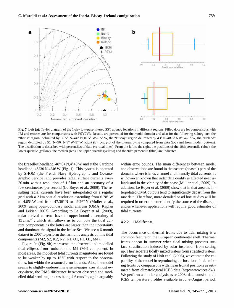
The combination of daily variations of atmospheric fluxesand weak winds can lead to strong SST diurnal anomalies(hereafter Dsst). The Dsst amplitudes are computed over a

24 h period as the difference between the maximum SST andthe minimum SST previously corrected from the daily trend(Pimentel et al., 2008). The Dsst for the buoy data are onlycomputed when the 24 SST values per day are available toavoid any miscalculations of the Dsst amplitudes.

Figure 7b displays box plots of the observed and the mod-elled Dsst amplitudes over the area covering the Bay of Bis-cay, the Celtic shelves and the North Sea (areas shown inFig. 3); it illustrates the distribution of data by showing dif-ferent values of Dsst amplitudes below which a certain per-centage of data are observed. Globally Dsst amplitudes areunderestimated in the model, and the median observed Dsstis 0.25◦C, while the median modelled Dsst is only 0.20◦C.When looking regionally at the distribution (not shown), wefound that Dsst is underestimated almost everywhere for the50 % of the data with smaller amplitudes (i.e. Dsst ampli-tudes below the median value). The resolution of the modeland of the forcing, the surface heat fluxes and the verticalmixing in the upper ocean are critical aspects for the diur-nal cycle modelling (Pimentel et al., 2008). According toBernie et al. (2005), a minimum of a 1 m vertical resolutionin the upper ocean and of a 3 h temporal resolution of sur-face fluxes is required to simulate 90 % of the observed Dsst.IBI is forced with 3 h atmospheric fields, but has a coarser



Fig. 5. Transports (outflow) in Sverdrup at the Strait of Gibraltar for TOV (transport observation velocity; the interface used to separate theinflow from the outflow is defined as the time-dependent depth of the surface of zero low-pass frequency velocity), TMV (transport modelvelocity) and TMS (transport model salinity; the outflow transport is computed using the commonly used 37.25 isohaline).

vertical resolution with 8 levels (18 levels) in the top 10 m(50 m), which only enables representation of 70 % of the Dsst(Bernie et al., 2005). This partly explains the underestimationof the Dsst in the model. Overestimated wind stress may alsolead to an underestimation of the Dsst by inducing too strongvertical turbulent mixing and preventing diurnal heating. Asfor lower frequencies (see previous section), we recommendfurther assessment on the realism of the wind field forcing.

3.4 Upper layer stratification

The upper layers stratification is a key process to represent ina regional model for its implications on circulation and ener-getics, in particular at the air–sea interface, and for its stronginfluence, or even coupling, with biological processes. Thesubsurface ocean is sparsely sampled with observations. Inthe Bay of Biscay, for instance, only two moorings of hourlytemperature and salinity (T/S) profiles are available to thecommunity (see Sect. 4.3.3). The UK MetOffice providesthe so-called EN3 dataset that gathers subsurfaceT/S pro-files from different sensors (e.g. ARGO floats) with qualitycontrol based on a comprehensive set of checks (Ingleby andHuddleston, 2007). Figure 8 illustrates the available data forFebruary and August 2008. The sampling is inadequate fora detailed investigation of the processes underlying theT/S

distribution. Instead it allows an overall view of the modelperformance in different areas.

Figure 8 shows the RMS of the model–data misfits in tem-perature over the upper 200 m. We also compute the mixedlayer depth (MLD) from the model and EN3 profiles usinga criterion on density and a threshold of 0.02 kg m−3 (notshown). In February, modelled temperatures show very goodagreement with data almost everywhere, with RMS globallylower than 0.5◦C. The profile of temperature RMS computedover the whole IBI domain (not shown) indicates that maxi-mum RMS values are reached between 50 and 130 m, whichis consistent with differences in modelled and observed MLD

at these depth ranges. In August, larger RMS in temperatureprofiles (up to 2◦C) are found on shelves as well as in thedeep ocean, with a model overestimation of the temperaturein the upper 200 m, in the Iroise Sea and in the English Chan-nel. The MLD is underestimated in the model in summer.

Besides the difficulty of single-point comparison (in par-ticular because of the mesoscale signals), these compar-isons emphasize the need to further test the vertical-mixingphysics: parameterization and values of parameters, as wellas forcing fields (impact of over- or underestimation of windforcing on turbulence). Another possible source of error maybe the wave-mixing parameterization coefficient. Sensitivityexperiments performed with a 1/12◦ resolution configurationhave shown that the modelled MLD (and consequently tem-peratures in the upper ocean layers) is very sensitive to thewave-mixing parameterization coefficient. The model MLDrepresentation can be enhanced by tuning this parameter,but the parameterization seems to be as inadequate in semi-enclosed seas as in the Mediterranean Sea or the North Sea.Thus the parameter used is a compromise to minimize theMLD errors both in the open ocean and in the semi-enclosedseas.

4 Regional skill assessment

4.1 Introduction

We now focus on the Bay of Biscay and explore the model–data consistency for processes specific to the shelf (Sect. 4.2)as well as slope and deep regions (Sect. 4.3). The surfacecirculation in the Bay of Biscay is relatively weak over theabyssal plain (a few cm s−1, Charria et al., 2011); it is mainlycyclonic in winter and anticyclonic in summer. Slope cur-rents have been evidenced off the northern Iberian coastand over the Armorican shelf break (Pingree and Le Cann,1990), with significant time variability (see Sect. 4.3.5 for the



Fig. 6. Comparison to satellite SST observations (◦C). From left to right: bias (model–observation), RMS error, observation standard devia-tions and model standard deviation. The first row shows annual statistics, the middle one shows statistics for winter and the bottom row forsummer. On each figure, the black line indicates the 200 m isobath.

Iberian Poleward Current). The circulation over the shelves isdominated by tidal currents; the residual currents are mostlywind-driven and are highly variable in time. Anticyclonicand cyclonic eddies are observed in the deep region; theymostly result from instabilities of the slope current develop-ing at capes and canyons (Pingree and Le Cann, 1992). In-ternal tides are generated in regions of interaction betweenbarotropic tidal currents and the shelf break. Two sites ofgeneration have been described in the literature: the Armor-ican shelf break around 47◦ N (Pairaud et al., 2010) and theGalician coast (Pichon and Correard, 2006).

We investigate the representation of these processes basedupon the available observations. The emphasis is on shelvesand slopes because of potential implication for users in biol-ogy or other downstream applications of the IBI system. We

also examine the representation of the Iberian Poleward Cur-rent flow along the northern Spanish coasts in winter. The ob-jective is to show that such a regional modelling system haspotential as a complement to observations (an integrated ap-proach) to give information on non-observed physical quan-tities and to provide links between observations.

4.2 Celtic shelves

4.2.1 Surface tidal currents in the Iroise Sea

In an attempt to locally investigate the performance of themodel at reproducing tidal surface ellipses in one particularregion characterized by intense tidal currents (up to 4 m s−1

in some interisland passages; SHOM, 1994), we use surfacecurrent data from the HF WERA (Wellen Radar) radars at



Fig. 7.Left (a): Taylor diagram of the 1-day low-pass-filtered SST at buoy locations in different regions. Filled dots are for comparisons withIBI and crosses are for comparisons with PSY2V3. Results are presented for the model domain and also for the following subregions: the“Iberia” region, delimited by 36.5◦ N–44◦ N,10.5◦ W–6.5◦ W, the “Biscay” region delimited by 43◦ N–48.5◦ N,8◦ W–1◦ W, the “Ireland”region delimited by 51◦ N–56◦ N,9◦ W–3◦ W. Right (b): box plot of the diurnal cycle computed from data (top) and from model (bottom).The distribution is described with percentiles of data (vertical lines). From the left to the right, the positions of the 10th percentile (blue), thelower quartile (yellow), the median (red), the upper quartile (yellow) and the 90th percentile (blue) are indicated.

the Brezellec headland, 48◦ 04 N,4◦40 W, and at the Garchineheadland, 48◦30 N,4◦46 W (Fig. 1). This system is operatedby SHOM (the French Navy Hydrographic and Oceano-graphic Service) and provides radial surface currents every20 min with a resolution of 1.5 km and an accuracy of afew centimetres per second (Le Boyer et al., 2009). The re-sulting radial currents have been interpolated on a regulargrid with a 2 km spatial resolution extending from 6.78◦ Wto 4.65◦ W and from 47.30◦ N to 49.26◦ N (Muller et al.,2009) using open-boundary modal analysis (OMA; Kaplanand Lekien, 2007). According to Le Boyer et al. (2009),radar-derived currents have an upper-bound uncertainty of15 cm s−1, which still allows us to compute the tidal cur-rent components as the latter are larger than the uncertaintyand dominate the signal in the Iroise Sea. We use a 6-monthdataset in 2007 to perform the harmonic analysis of nine tidalcomponents (M2, S2, K2, N2, K1, O1, P1, Q1, M4).

Figure 9a (Fig. 9b) represents the observed and modelledtidal ellipses from runbc for the M2 (M4) component. Inmost areas, the modelled tidal currents magnitudes are foundto be weaker by up to 15 % with respect to the observa-tions, but within the assumed error bounds. Also, the modelseems to slightly underestimate semi-major axes almost ev-erywhere, the RMS difference between observed and mod-elled tidal semi-major axes being 4.6 cm s−1, again arguably

within error bounds. The main differences between modeland observations are found in the eastern (coastal) part of thedomain, where islands channel and intensify tidal currents. Itis, however, known that radar data quality is affected near is-lands and in the vicinity of the coast (Muller et al., 2009). Inaddition, Le Boyer et al. (2009) show that in that area the in-terpolated OMA outputs tend to significantly depart from theraw data. Therefore, more detailed or ad hoc studies will berequired in order to better identify the source of the discrep-ancies whenever applications will require good estimates oftidal currents.

4.2.2 Tidal fronts

The occurrence of thermal fronts due to tidal mixing is acommon feature on the European continental shelf. Thermalfronts appear in summer when tidal mixing prevents sur-face stratification induced by solar insolation from settingup. They separate tidally mixed waters from stratified waters.Following the study of Holt et al. (2008), we estimate the ca-pability of the model in reproducing the location of tidal mix-ing fronts by comparisons with mean frontal positions as esti-mated from climatological ICES data (http://www.ices.dk/).We perform a similar analysis over 2008: data consist in allICES temperature profiles available in June–August period,


http://www.ices.dk/


Fig. 8. RMS of temperature differences between EN3 profiles and model profiles computed over the first 200 m. Results are presented forFebruary 2008(a) and August 2008(b). On each figure, the black line indicates the 200 m isobath.

and mean tidal fronts are deduced from the observed surfaceto bottom difference defined by1T = 0.5◦C. The same ap-proach is applied to model temperature profiles. Results arepresented in Fig. 10. Over the shelf, SST fronts are due tothe vertical turbulent mixing generated by tidal stresses at theseabed; the model shows reasonable agreement with observa-tions in the main tidal front positions over the shelf, particu-larly for the Ushant front (northwest coast of Brittany), at theentrance of the English Channel, in the northern Irish Sea, offNorth Scotland and south of Doggar Bank (along∼ 54◦ N).MODIS SST data have also been used to perform qualita-tive comparisons of the SST fronts (Fig. 11). The modelledSST shows very good agreement with observations in themain tidal front positions. Over the shelf, the model presentslarger stratified regions in the Irish Sea and colder SST in theUshant front (off West Brittany) and at the entrance of theEnglish Channel. Elsewhere SST fronts are relatively wellrepresented both in temperature and in extension. On theArmorican shelf break, internal tides induce strong verticalmixing, which prevents the formation of seasonal stratifica-tion and results in a cold SST tongue along the shelf breakfrom 11◦ W to 5◦ W. The cold intrusion is also reproducedin the model: temperature is underestimated by 0.5◦C andthe southeastward extension is relatively well represented.The relatively good accuracy of the model in reproducingthese tidal mixing fronts is mainly related to the good repre-sentation of the bottom stress which affects the propagation

of barotropic tidal waves,the k–epsilon two-equation modelcombined with the closure model of Canuto et al. (2001),the limitation of the dissipation under stable stratification andthe tracers’ advection (Holt et al., 2008). The model presentsweaker stratification over Doggar Bank and to the west ofEngland, and summer stratification is overestimated in thesouthern Irish Sea. Differences with observed mean frontalpositions are also seen southwest of Denmark. Salinity strat-ification is important in this region (two major rivers includ-ing the Elbe river) and may impact frontal position (Holt etal., 2008).

4.2.3 Surges

For verification purposes, we diagnose the model’s ability toreproduce surges by comparing residual elevations (i.e. de-tided sea levels) from the model with in situ measurementsat time scales shorter than 10 days. At these time scales, thesimulated coastal sea level is the signature of the static andnon-static response to atmospheric pressure, of the responseto wind forcing and of tidal interactions (see, for instance,Carrere and Lyard, 2003). The in situ sea level dataset con-sists of 115 tide gauges located along the European coasts(see red dots on Fig. 1). The harmonic analysis tool fromPuertos del Estado is used to compute the tidal componentfrom tide gauge elevations and to predict the tidal elevations;this software was developed to be used within the ENSURF



Fig. 9. (a) and (b): M2 (a) and M4 (b) modelled (black) and ob-served (red) surface tidal ellipses at HF radar measurements loca-tions. Shaded contours represent the model–observation differencefor semi-major axis (cm s−1). (c) Modelled (black) and observed(red) near-surface M2 tidal ellipses at Puertos del Estado current-meter locations. Shaded contours: M2 surface velocity differencebetween the run with stratification (runbc) and the run without strat-ification (runbt). On each figure, the black line indicates the 200mbathymetry isoline.

ensemble system (Perez et al., 2012) and is based on Fore-man (1977) harmonic analysis software.

Comparisons between residual elevations from the modeland the observations are shown in Fig. 12 for the Bay of Bis-cay and the English Channel. The elevations due to the staticresponse of the ocean to atmospheric pressure (the so-calledinverse barometer or IB effect) alone have been included inthe comparison. The model shows very good agreement withdata: 90 % (67 %), of RMS differences are smaller than 5 cm( 3 cm), and 80 % of correlations are greater than 0.9 (re-sults from detailed comparisons between observed and mod-eled values; results only synthesized on Fig. 12) and it per-forms better than the IB response (54 % with RMS differ-ence smaller than 5 cm). It is most effective at high latitudes,which are more energetic areas, and where the ocean dynam-ical space and time scales are smaller, while at midlatitudes

Fig. 10. Summer (June, July, August) tidal front positions asdeduced from surface to bottom temperature difference (1T =0.5◦C) from the model (red) and from ICES data (black).

the model response to atmospheric forcing is closer to the IBapproximation (not shown).

4.3 IBI shelf breaks and deep ocean

4.3.1 Surface tidal currents over the slope

Surface tidal currents from runbc are compared to observedcurrents at buoy stations along the northern Iberian coast forthe M2 constituent (Fig. 9c). The model tends to overesti-mate the current amplitudes almost everywhere. The largestdifferences are found at Villano-Sisargas: the modelled el-lipse azimuth is remarkably consistent with the observations,but the modelled semi-major axis is more than twice as largeas the observed one. Garcıa-Lafuente et al. (2006) also foundthe M2 barotropic tidal currents were much greater than ex-pected in this area; they attributed it to internal tides of con-siderable amplitudes. Pichon and Correard (2006) showedthat the northwest Spanish continental slope is indeed an areaof internal tide generation. In the vicinity of Villano-Sisargas,differences of the M2 surface current amplitudes between therun with stratification (runbc) and the run without stratifica-tion (runbt) present high values due to internal tides (Fig. 9c).As internal tide generation is very sensitive to the bathymetrygradient and as the bottom topography and the coastline ge-ometry are complex in the Cape Finisterre area, we expect er-rors in the slope position in the model bathymetry to explainthe differences observed at this station. Without any betterestimate of the local bathymetry, we cannot further test this



Fig. 11.Sea surface temperature (◦C) from MODIS data(a) and from the model(b) on 27 September 2008.

hypothesis. At Cabo Silleiro, tidal ellipse parameters are notcorrectly modelled. The model ellipse inclination is parallelto the isobaths, which is consistent with the study of Visser etal. (1994) in well-mixed conditions. Visser et al. (1994) alsoshowed that in a region of freshwater influence, the stratifica-tion significantly influences the cross-shore component thatcan reach 40 % of along-shore component; this is consistentwith the observed ellipse orientation. At Donostia and Matx-itxako, modelled ellipses are also oriented along the slope,while observed ones are oriented across the slope. Indeed, thevertical profile of the observed M2 semi-major axis shows aclear stratification in the surface layers which is not repre-sented in the model (Fig. 13). Below this layer (upper 30 m)the modelled profile is in good agreement with observationsfor the two current profiles. As discussed in Sect. 4.3.3, thesurface layer’s salinity suffers from an over- or underestima-tion in the model with respect to observations (Fig. 14).

It should be stressed that model–data comparisons at sin-gle locations are very challenging in the sense that the mod-elled field can vary a lot from one grid point to the other,especially in the slope area. Indeed, a small local error in thebathymetry (depth and slope) can generate large displace-ments of the circulation patterns. Therefore, such compar-isons are not necessarily representative of the overall modelperformance. Here, we presented them to illustrate somephysical processes at work in order to explain the model–data discrepancies.

4.3.2 Internal tides

We use 10 yr of TOPEX/Poseidon data combined with 7 yrof Jason-1 altimeter data spanning the period from Septem-ber 1992 to January 2009 to obtain estimates of the inter-nal tide signature in sea surface elevation. Altimetric data arenot used for the validation of barotropic tides, as barotropictides are compared to the FES2004 solution which assimi-lates altimetric data. The fraction of internal tides which isphase-locked with astronomical potential has sufficient co-herence in both space and time for its surface signal to be de-tected in altimetric multi-year time series (Ray and Mitchum,1997). We use an along-track harmonic analysis product pro-vided by CTOH/LEGOS (F. Lyard, personal communica-tion, 2010) to estimate the temporally coherent M2 com-ponent. We work with TOPEX/Poseidon/Jason1 track 137that crosses the Armorican shelf slope at nearly a right an-gle (Fig. 1) as we expect the M2 internal tides to propagatealmost in the same direction (internal tides propagate per-pendicular to the shelf break, Pairaud et al., 2010). To sepa-rate the barotropic tides from the time-coherent internal tidesignal, we then spatially filter the M2 real and imaginaryparts so that we remove the barotropic large-scale signal (Rayand Mitchum, 1997). According to Pairaud et al. (2010), thewavelengths of baroclinic mode 1 and mode 2 are respec-tively 141 km and 75 km in the abyssal plain. Note that thesevalues have been obtained using data collected during the pe-riod September–October 1994 and may vary with the strati-fication. To take into account the angle between the altimeter



Fig. 12. Taylor diagram for comparisons between tide gauge dataand the model residual elevations (blue) and the inverse barometer(red). Results are computed for periods below 10 days and for datalocated in the Bay of Biscay and in the English Channel. The ra-dial coordinate indicates the standard deviation normalized by thedata standard deviation; the concentric circles represent the RMSdifferences for time series normalized by the data standard devia-tion (the observations are indicated with the black point), and theangular coordinate represents the correlation with observations.

track and the internal tide direction of propagation we use aspatial cut-off slightly larger than the wavelength. We alsofilter at shorter scales to reduce the altimeter noise. Finally,along-track tidal components are filtered between 140 kmand 210 km for mode 1 and between 60 km and 110 km formode 2. The “residual tides” are obtained by removing thefiltered signal from the harmonic components.

Figure 15 presents the along-track amplitude and phaseas computed from the altimetric data and from the modelfor mode 1 and for mode 2. It also presents the along-trackbathymetry. Indications attesting that the small oscillationsare internal tides are as follows: (1) oscillations are gener-ated in the Armorican shelf slope region (45.8◦ N–46.0◦ N);(2) south of the shelf break the phase increases constantlyin the Bay of Biscay, which indicates that the wave prop-agates away from the shelf; and (3) for mode 1 and mode2 we find wavelengths of approximately (λ1, λ2) = (197 km,76 km) in the altimetric data and the model; these values areslightly larger but in good agreement with theoretical values.The agreement between the altimetric and model estimatesis remarkable: the misfits lie between 1 and 2 cm for the to-

Fig. 13. Vertical profiles of the M2 semi-major axis (cm s−1) asobserved (dashed line) and modelled (full line) at the Matxitxakobuoy location.

tal M2 amplitude and the model presents similar wavelengthsthan altimetric data. Interestingly, both the model and data in-dicate that the first mode does not have the dominant surfacesignature in the Bay of Biscay. Minor discrepancies in thebaroclinic amplitudes and phases are, however, observed. Formode 1 (mode 2) there is a southward (northward) shift of themodel sea surface signal. For the two modes, model ampli-tudes are slightly overestimated, especially near the genera-tion site for mode 2. As previously mentioned, errors in themodel bathymetry (here for the Armorican shelf slope rep-resentation) are expected to lead to uncertainties in the tidalrepresentation, especially close to the generation sites of in-ternal tides.

4.3.3 Local stratification off the Basque Country

The Donostia and Matxitxako deep-sea buoys deployed byAZTI-Tecnalıa over the slope off the Basque Country pro-vide hourly measurements of atmospheric parameters andocean temperature and salinity from 10 to 200 m (Rubioet al., 2013; Fig. 1, Table 4). They represent very valuabledata as they are the only available time series of tempera-ture and salinity profiles over such a long period. The timeevolutions of temperature and salinity as observed and mod-elled at the Matxitxako station are presented in Fig. 14. The



Fig. 14.Temperature (◦C) and salinity (psu) profiles in the upper 200 m at station Matxitxako as a function of time (August 2007 to February2009) from the observations(a, b) and from the model(c, d). As no measurement is available above 10 m, we show the model results below10 m.

profiles show clear seasonal stratification. The model repro-duces reasonably well the rapid heating and freshening ofspring 2008. The cooling and mixed-layer deepening duringwinter are also correctly represented. However, the modelunderestimates the MLD equivalent in winter (The MLDequivalent is computed as the depth at which the densitychanges from the density at 10 m by 0.02 kg m−3; results notshown). In summer 2007 we also notice that the model salin-ity is too low in the upper layers. This is due to the initial-ization from PSY2V3, which is too fresh in this region. Onthe contrary, the model is slightly saltier in the surface lay-ers during summer 2008. However, rapid freshening pulsesduring September 2008 are well represented in the model.Surface salinity uncertainties reflect mainly those on the pre-cipitation fields; the latter are unknown but are expected to belarger in coastal areas such as northern Iberia because of oro-graphic effects. Furthermore, Ferrer et al. (2009) have shownthat fresh water discharge from several Spanish rivers can im-

pact the offshore salinity conditions under specific oceano-meteorological conditions.

During the winter of 2007–2008, the ocean becomeswarmer and saltier over the whole water column. This phe-nomenon is more marked in the model and affects the 350 mupper layer: it corresponds to a warm extension of the IberianPoleward Current, also called the “Navidad event” (Pin-gree and Le Cann, 1992). This pattern is discussed later inSect. 4.3.5.

4.3.4 Residual currents

Data used for comparisons consist of residual currents fromthe surface buoys of Puertos del Estado (Table 4). Fig-ure 16 shows the observed and modelled residual currentsat Bilbao (zonal component), Estaca de Bares (zonal compo-nent) and at Cabo Silleiro (meridional component). Both dataand model time series are detided, filtered below 25 h andone-day-averaged. The results show that modelled residual



Fig. 15. (a)Along-track amplitudes (cm) deduced from the M2 har-monic analysis of altimetric data (red) and model (black).(b) Baro-clinic amplitudes in cm and(c) phase of the residual tides for thealtimetric data (red) and the model (black) and for the first baro-clinic mode. (d) Baroclinic phased-locked elevations in cm and(e) phase of the residual tides for the altimetric data (red) and themodel (black) and for the second baroclinic mode.(f) Along-trackbathymetry (m).

currents have some discrepancies when currents are weak,but they are relatively well reproduced elsewhere. Howeverthe model tends to overestimate peak currents. Along theIberian Coast, RMS errors vary between 5.8 and 9.1 cm s−1.Comparisons between wind speed observed at buoy stationsand extracted from ECMWF fields indicate that magnitudesare significantly higher in the ECMWF fields, especially dur-ing strong wind events (not shown). Along the Iberian coast,the main current component is the along-shore component:currents are predominantly meridional at the Cabo Silleirostation, while they have a predominant zonal orientation atEstaca de Bares, Cabo Penas and Bilbao. This distribution ofresidual currents is well reproduced in the model. North ofSpain, both observations and the model show clear eastwardcurrent intensifications during January. They are overesti-mated in the model and spread over a larger period. These in-tensifications are associated with the extension of the Iberian

Fig. 16.Modelled (black) and observed (red) residual near-surfacevelocity (approximately along slope) at various moorings along theIberian slope (cm s−1): northern component at Cabo Silleiro, andeastward component at Estaca de Bares and Bilbao.

Poleward Current along the northern Spanish coast. In sum-mer, some current pulses are also observed in the data frommid-June to late August 2008, and are well reproduced in themodel.

4.3.5 A focus on the circulation in the southern Bay ofBiscay

We now focus on the ability of the model in reproducinga typical dynamic feature of the southern Bay of Biscay:the warm extension of the Iberian Poleward Current alongthe northern Spanish coast during winter. In this sectionour objective is not consistency assessment; we analyse sev-eral variables or quantities that are relevant for the Navi-dad occurrence (e.g. temperature and salinity anomalies inthe upper layers, poleward along-slope currents) and showhow the model can be used as a complement to available



Fig. 17.Sea surface temperature (◦C) from AVHRR data(a) and from the model(b)for 20 January 2008. Modelled temperature at 200 mdepth for 20 January 2008(c).

observations. The analysis of the modelled SST and sea sur-face salinity (SSS) in the Bay of Biscay shows a warm andsalty current flowing poleward along the western and thenorthern Iberian Peninsula and reaching the southwesternFrench coasts during winter of 2007–2008 (Fig. 17, SSS notshown; see also wintertime salinity anomalies on Fig. 14).The extension of the Iberian Poleward Current at or near sur-face along the northern Iberian coast is a recurrent feature ofthe autumn/winter circulation of the Bay of Biscay (Frouinet al., 1990; Garcia-Soto et al., 2002; Le Cann and Serpette;2009) and has been referred to as the “Navidad event” (Pin-gree and le Cann, 1992). The extension of the IPC and the as-sociated warming are, however, very variable from one yearto the other; furthermore, it also undergoes some variabil-ity at timescales of a few days, as discussed below. Its mainsignature is a surface warming along the coast as it carriespoleward warm water masses from the western Iberian re-gion. Satellite observations clearly show the warm intrusionof the Iberian Poleward Current extending poleward as faras the Cantabrian shelf slope north of Spain on 20 January2008 (Fig. 17). The intrusion is represented by a similar spa-tial extent in IBI with its leading edge reaching 3.5◦ W at thesame date. Modelled SST is slightly warmer than observedSST within the Iberian Poleward Current and in surroundingwaters; moreover, the warm tongue appears to be narrowernorthwest of Spain. At the surface, the current thermal sig-nature is about 1◦C warmer than adjacent waters in the dataand in the model. It decreases poleward, varying from morethan 14.5◦C off northwest Spain to about 13.5◦C at 3◦ W.This corresponds to a drop of 1◦C over a∼ 450 km distance,which is in good agreement with the poleward temperaturegradient obtained by Frouin et al. (1990) using satellite SSTdata. The current narrows from 40 km off northwest Spainto less than 30 km at 3◦ W. Vertical across-slope sections of

thermohaline fields along the warm current (not shown) in-dicate the core of warm and salty water flows over the uppershelf slope, and extend from the surface to 350 m. The tem-perature field structure is illustrated with the map of 200 mtemperature (Fig. 17).

Comparisons between modelled and observed along-sloperesidual currents (Fig. 16) indicate that the time variabilityof currents in the model is in reasonable agreement withdata. They also suggest that the model tends to overesti-mate the IPC surface currents at the Puertos del Estado buoys(e.g. Cabo Silleiro and Estaca de Bares). At Bilbao (Fig. 16)the eastward pulses in February and March are not observed;this suggests that the IPC may be penetrating too far into theBay of Biscay in the model. The analysis of other Navidadevents (i.e. over other years) should be necessary to deter-mine whether the model overestimation of the zonal exten-sion of the IPC is a systematic bias in this configuration or ifit occurred specifically for these events of February–March2008.

The warm current transport has been estimated along theslope for sections perpendicular to the flow (see definition inthe caption of Fig. 18). Considering typical temperature andsalinity values along the current in the model, the transporthas been computed for water masses warmer than 13.0◦Cand saltier than 35.7 psu. Note that these values do not takeinto account the spatial gradient of temperature and salin-ity in the flow. The transport time evolution is shown inFig. 18a. The warm intrusion is established in October 2007northwest of Spain (Galicia). The flow progresses eastwardalong the slope around Cape Finisterre, reaches the coast offnorth Galicia in November and continues its intrusion in theCantabrian Sea. North of Spain, the warm current is estab-lished until May. From the transport across each section weestimate the mean poleward flow to propagate at velocities



Fig. 18. (a) Transport (Sv) of the poleward flow for water masswarmer than 13.0◦C and saltier than 35.7 psu at 43.24◦ N (blue),7.61◦ W (turquoise blue), 6.2◦ W (green), 3.8◦ W (yellow) and44.4◦ N (orange).(b) Meridional wind stressτy (Pa) off westernIberia (red) and of the zonal wind stressτx off northern Iberia(blue). Boxes chosen for the spatial average ofτx andτy have beenchosen following the study of Le Cann and Serpette (2009).

between 13 and 24 cm s−1, which agree with typical val-ues published (Frouin et al., 1990; Garcia-Soto et al., 2002).From Fig. 18a, we also notice the warm current transport ishighly variable at periods of a few days and may vary fromno transport to more than 2 Sv over a short period. Such vari-ability at daily timescales has been described by Herbert etal. (2011) during the winter of 2004 from in situ observa-tions and a numerical simulation. These authors suggest thatthe high-frequency variations are due to local wind forcing.When it is established, the current varies almost simultane-ously at each section in response to forcing. The transporttime series present a lag of 1 day between 8◦ W and 6◦ W(6◦ W and 3.8◦ W) and correlation of 0.75 (0.79) betweenthe two transports.

Driving mechanisms of the poleward current are often at-tributed to the large-scale meridional pressure gradient inthe North Atlantic and to local wind stress (Frouin et al.,1990; Le Cann and Serpette; 2009). Figure 18b representsthe meridional wind stress off western Iberia and of the

zonal wind stress off northern Iberia averaged over boxes de-fined following Le Cann and Serpette (2009). Positive valuesof wind stress indicate downwelling-favourable conditionswhich are likely to force the poleward flow. West of Iberia,wind stress is upwelling favourable until October 2007; thenit is northward until the end of the year and is expected toprovide a driving mechanism of the poleward current. Whenthe current has reached Cape Finisterre and turns eastward,its poleward flow is maintained by eastward winds.

5 Conclusions

A high-resolution simulation covering the Iberia–Biscay–Ireland (IBI) region was carried out over the period of July2007–February 2009 within the MyOcean project (Cailleauet al., 2012). In this paper, we had three main objectives: (1)to give an overview of the model configuration used for thesimulation; (2) to give a broad-brush account of one particu-lar aspect of this work, namely consistency verification; thistype of validation is conducted upstream of the implementa-tion of the system before it is used for production and rou-tinely validated; it is meant to guide model development inidentifying gross deficiencies in the modelling of several keyphysical processes; and (3) to show that such a regional mod-elling system has potential as a complement to patchy obser-vations (an integrated approach) to give information on non-observed physical quantities and to provide links betweenobservations by identifying broader-scale patterns and pro-cesses. Objectives (2) and (3) were pursued in the year 2008.

We then examined domain-wide consistency verificationresults in terms of barotropic tides, transports, sea surfacetemperature and stratification. We also focused with moredetail on two dynamical subregions: the Celtic shelves andthe Bay of Biscay slope and deep regions; there, the model–data consistency was checked, not exhaustively, but for a fewimportant variables and processes such as tidal currents, tidalfronts, internal tides and residual elevation. Although a num-ber of relatively minor points have been raised in the paperand some of these points are not in the IBI system specifi-cations (e.g. details of the MW outflow), no major discrep-ancy with respect to expectations was identified. However,the study highlighted a few grey areas requiring more specificattention and testing, as well as priorities for improvement.

For instance, the analysis of the tidal elevations and currentfields suggests that local improvements in the bathymetry areessential to better represent the tidal propagation, the bot-tom mixing and the generation of internal tides. Such im-provements are also essential in regions of downscaling tofiner-grid models, as well as to facilitate point comparisonswith observations, a small error in the bathymetry (depth andslope) being able to generate large displacements of the cir-culation patterns.

Another important forcing in coastal areas is freshwaterdischarge, mainly from rivers. The analysis of the baroclinic



tidal surface signal points out at least two regions in the Bayof Biscay where the surface stratification in the model wasprobably poorly represented (however, the lack of availablesubsurface hydrological data will not permit direct compar-isons). In these regions and according to past studies (e.g.Ferrer et al., 2009), runoffs from the Galician and the Basquerias have a significant impact on the local stratification butare not taken into account in our model configuration. Testsare necessary to quantify the impact of local changes ofthe surface stratification at different timescales on the baro-clinic tidal currents. More generally, it becomes evident thata large effort for a more realistic representation of continen-tal water discharge including the runoffs from small rivers isneeded at least in these areas. Following some of our consis-tency checks, daily runoffs (instead of monthly climatologi-cal ones) are now prescribed in the operational version of thisIBI configuration.

Other points follow. Further increases in horizontal andvertical resolution would allow for some types of applica-tions to be better served, such as biological connectivityand surface currents, the latter being probably strongly in-fluenced by wave–current interactions (Law-Chune et al.,2013). Further tuning of the bottom friction and its spatialdependence on the seabed type may improve the solutionlocally for tides and surges, with impacts on SST distribu-tion in frontal regions. Uncertainties in atmospheric forcingsare likely to drive model errors on surface circulation and ontracer distributions via wind-driven turbulence. Errors are ex-pected to occur for high frequencies and small-scale patterns,especially close to the coasts where the effects of small-scale orography are poorly represented. Stochastic modellingwould provide an interesting framework for the assessmentof the impacts of atmospheric uncertainties (e.g. Quattroc-chi et al., 2013). We also suggest that R&D studies shouldbe carried out to accompany the development of atmosphericdownscaling for operational systems.

The model–data comparisons presented in this paper didnot include an error analysis; for this, we need reliable esti-mates of uncertainties on the data, which are generally un-available. Such estimates are required, for instance, in or-der to better identify the source of the discrepancies betweenthe simulations and the gridded HF radar data in the vicin-ity of the Ushant front. The representativeness of local mea-surements (such asT/S profiles from the EN3 database orcurrent time series from the Puertos del Estado buoy net-work) is a general problem, linked to the problem of upscal-ing local information when comparing to increasingly high-resolution simulations. We also suggest to complement thedatasets used for the consistency checks: for example, bothFerryboxT/S data and satellite altimetry data would be anice complement, both datasets being characterized by repet-itive sampling.

In the last section of this paper, we investigated the repre-sentation of the winter slope current along the northern Span-ish coast (Navidad event). As very few data were available,

this test is an illustration of the potential of our modellingsystem as a complement to observations within an integratedapproach. We examined diagnostics on observed (e.g. sur-face currents) and non-observed (e.g. along-slope transport)quantities that could serve as a basis to define indices andthat provide links between observations.

Lastly, the relatively high (2–3 km) horizontal resolu-tion used clearly pushes the model into the sub-mesoscale-permitting regime over much of the domain and allows for asignificant part of the internal wave spectrum to be resolved.This seems to be the natural way forward to anticipate futurehigh-resolution satellite observing systems such as SWOT(Surface Water and Ocean Topography).

Acknowledgements. The research leading to these results havereceived funding from the European Community’s SeventhFramework Programme FP7/2007-2013 under grant agreementno. 218812 (MyOcean) and through its partnership with CNRS(Centre National de la Recherche Scientifique).

The regional bathymetries used for the study have been providedby Ifremer, the French Navy Hydrographic and Oceanographic Ser-vice (Service Hydrographique et Oceanographique de la Marine,SHOM) and the North West Shelf Operational Oceanographic Sys-tem. Tide gauge data used were provided by Puertos del Estado, theMarine Institute and the Danish Meteorological Institute; and tidegauge data from SHOM, the British Oceanographic Data Centre andGLOSS were provided by Collecte Localisation Satellites (CLS).The MODIS SST image was obtained through the online JPLPO.DAAC Ocean ESIP Tool (POET) at the Physical OceanographyDistributed Active Archive Center (PO.DAAC), NASA Jet Propul-sion Laboratory, Pasadena, CA (http://podaac.jpl.nasa.gov/poet).

The authors gratefully acknowledge the receipt of buoy data fromPuertos del Estado, Meteo France, the Marine Institute and the Ma-rine Institute and AZTI-Tecnalia, as well as along-track altimet-ric data from LEGOS/CTOH, historical current-meter data fromBODC and radar HF data provided by Fabrice Ardhuin and SHOM.

Outflow estimates at the Strait of Gibraltar have been obtainedthrough the monitoring station at Espartel sill, west Gibraltar, whichis deployed and serviced within the frame of the Spanish-fundedprojects INGRES (REN2003-01608, CTM2006-02326, CTM2009-05810E and CTM2010-21229). We acknowledge J. Garcia La-fuente, PI of these projects, for providing us with this information.

We thank the Mercator Ocean teams, Charly Reignier and ClementBricaud, whose hard work made this study possible. This study alsobenefited from fruitful discussions with Gildas Cambon concerningthe Ushant thermal front.

Edited by: A. Schiller

The publication of this articleis financed by CNRS-INSU.


http://podaac.jpl.nasa.gov/poet


References

Adcroft, A. and Campin, J.-M.: Rescaled height coordinates for ac-curate representation of free-surface flows in ocean circulationmodels, Ocean Model., 7, 269–284, 2004.

Alvarez, M., Perez, F. F., Bryden, H. L., and Rios, A. F.:Physical and biochemical transports structure in the NorthAtlantic subpolar gyre, J. Geophys. Res., 109, C03027,doi:10.1029/2003JC002015, 2004.

Arbic, B. K., Wallcraft, A. J., and Metzger, E. J.: Concurrent sim-ulation of the eddying general circulation and tides in a globalocean model, Ocean Model., 32, 175–187, 2010.

Barnier, B., Madec, G., Penduff, T., Molines, J.-M., Treguier, A.-M., Le Sommer, J., Beckmann, A., Biastoch, A., Boning, C.,Dengg, J., Derval, C., Durand, E., Gulev, S., Remy, E., Talandier,C., Theetten, S., Maltrud, M., McClean, J., and De Cuevas, B.:Impact of partial steps and momentum advection schemes ina global ocean circulation model at eddy-permitting resolution,Ocean Dynam., 56, 543–567, doi:10.1007/s10236-006-0082-1,2006.

Becker, J. J., Sandwell, D. T., Smith, W. H. F., Braud, J., B.Binder, B., Depner, J., Fabre, D., Factor, J., Ingalls, S., Kim,S.-H., Ladner, R., Marks, K., Nelson, S., Pharaoh, A., Trim-mer, R., Von Rosenberg, J., Wallace, G., and Weatherall, P.:Global bathymetry and elevation data at 30 arc seconds resolu-tion: SRTM30 PLUS, Mar Geod., 32, 355–371, 2009.

Benzhora, M. and Millot, C.: Characteristics and circulation of thesurface and intermediate water masses off Algeria, Deep-SeaRes., 42, 1803–1830, 1995.

Bernie, D. J., Woolnough, S. J., Slingo, J. M., and Guilyardi,E.: Modelling diurnal and intraseasonal variability of the oceanmixed layer, J. Climate, 18, 1190–1202, 2005.

Blayo, E. and Debreu, L.: Revisiting open boundary conditionsfrom the point of view characteristic variables, Ocean Model.,9, 231–253, 2005.

Brown, J. and Gmitrowitz, E. M.: Observations of the transversestructure and dynamics of the low frequency flow through theNorth Channel of the Irish Sea, Cont. Shelf Res., 15, 1133–1156,1995.

Brown, J., Carrillo, L., Fernanda, L., Horsburgh, K. J., Hill, A. E.,Young, E. F., and Medler, K. J.: Observations of the physicalstructure and seasonal jet-like circulation of the Celtic Sea andSt. George’s Channel of the Irish Sea, Cont. Shelf Res., 23, 533–561, 2003.

Burchard, H., Deleersnijder, E., and Stoyan, G.: Some numerical as-pects of turbulence-closure models, in Marine Turbulence: Theo-ries, Observations, and Models. Results of the CARTUM Project,Cambridge University Press, 2005.

Cailleau, S., Chanut, J., Lellouche, J.-M., Levier, B., Maraldi, C.,Reffray, G., and Sotillo, M. G.: Towards a regional ocean fore-casting system for the IBI (Iberia-Biscay-Ireland area): develop-ments and improvements within the ECOOP project framework,Ocean Sci., 8, 143–159, doi:10.5194/os-8-143-2012, 2012.

Candela, J.: The Gibraltar Strait and its role in the dynamics of theMediterranean Sea, Dynam. Atmos. Oceans, 15, 267–300, 1991.

Canuto, V. M., Howard, A. M., Cheng, Y., and Dubovikov, M. S.:Ocean turbulence. Part I: one-point closure model momentumand heat vertical diffusivities, J. Phys. Oceanogr., 31, 1413–1426,2001.

Carrere, L. and Lyard, F.: Modelling the barotropic response ofthe global ocean to atmospheric wind and pressure forcing –comparisons with observations, Geophys. Res. Lett., 30, 1275,doi:10.1029/2002GL016473, 2003.

Charria, G., Lazure, P., Le Cann, B., Serpette, A., Reverdin G.,Louazel, S., Batifoulier, F., Dumas, F., Pichon, A., and Morel,Y.: Surface layer circulation derived from Lagrangian drifters inthe Bay of Biscay, J. Mar. Syst., 109–110, Supplement S60–S76,doi:10.1016/j.jmarsys.2011.09.015, 2011.

Craig, P. D. and Banner, M. L.: Modeling wave-enhanced turbu-lence in the ocean surface layer, J. Phys. Oceanogr., 24, 2546–2559, 1994.

Coelho, H. S., Neves, R. J. J., White, M., Leitao, P. C., and Santos,A. J.: A model for ocean circulation on the Iberian coast, J. Mar.Syst., 32, 153–179, 2002.

Davies, A. M. and Aldridge, J. N.: A numerical model study ofparameters influencing tidal currents in the Irish Sea, J. Geophys.Res., 98, 7049–7067, 1993.

Davies, A. M., Kwong, S. C. M., and Flather, R. A.: A three-dimensional model of diurnal and semidiurnal tides on the Eu-ropean shelf, J. Geophys. Res., 102, 8625–8656, 1997.

Drevillon, M., Bourdalle-Badie, R., Derval, C., Drillet, Y., Lel-louche, J.-M., Remy, E., Tranchant, B., Benkiran, M., Greiner,E., Guinehut, S., Verbrugge, N., Garric, G., Testut, C.-E., La-borie, M., Nouel, L., Bahurel, P., Bricaud, C., Crosnier, L., Dom-browsky, E., Durand, E., Ferry, N., Hernandez, F., Galloudec, O.,Messal, F., and Parent, L.: The GODAE Mercator-Ocean globalocean forecasting system: results, applications and prospects, J.Oper. Oceanogr., 1, 51–57, 2008.

Dombrowsky, E., Bertino, L., Brassington, G. B., Chassignet, E.P., Davidson, F., Hurlburt, H. E., Kamachi, M., Lee, T., Martin,M. J., Mei, S., and Tonani, M.: GODAE systems in operation,Oceanography, 22, 80–95, 2009.

Egbert, G., Bennett, A., and Foreman, M.: TOPEX/Poseidon tidesestimated using a global inverse model, J. Geophys. Res., 99,24821–24852, 1994.

Ellett, D. J. and Martin, J. H. A.: The physical and chemicaloceanography of the Rockall Channel, Deep-Sea Res., 20, 585–625, 1973.

Fanjul, E. A., Gomez, B. P., and Rodriguez, I.: A description of thetides in the Eastern North Atlantic, Prog. Oceanogr., 40, 217–244, 1997.

Ferrer, L., Fontan, A., Mader, J., Chust G., Gonzalez, M., Valencia,V., Uriarte, A., and Collins, M. B.: Low-salinity plumes in theoceanic region of the Basque Country, Cont. Shelf Res., 29, 970–984, doi:10.1016/j.csr.2008.12.014, 2009.

Flather, R. A.: A tidal model of the North-East Pacific, Atmos.Ocean, 25, 22–45, 1987.

Foreman, F. G. G.: Manual for tidal heights analysis and predic-tions, Institute of Ocean Sciences, Patricia Bay, Pacific MarineReport, 77, 101 pp., 1977.

Frail-Nuez, E., Plaza, F., Hernandez-Guerra, A., Vargas-Yanez,M., and Lavin, A.: Mass transport in the Bay of Biscayfrom an inverse bix model, J. Geophys. Res., 113, C06023,doi:10.1029/2007JC004490, 2008.

Frouin, R., Fiuza, A. F. G., Ambar, I., and Boyd, T.: Observationsof poleward surface current off the coasts of Portugal and Spainduring winter, J. Geophys. Res., 95, 679–691, 1990.


http://dx.doi.org/10.1029/2003JC002015

http://dx.doi.org/10.1007/s10236-006-0082-1

http://dx.doi.org/10.5194/os-8-143-2012

http://dx.doi.org/10.1029/2002GL016473

http://dx.doi.org/10.1016/j.jmarsys.2011.09.015

http://dx.doi.org/10.1016/j.csr.2008.12.014

http://dx.doi.org/10.1029/2007JC004490


Garcıa-Lafuente, J., Dıaz del Rıo, G., and Sanchez Berrocal, C.:Vertical and bottom intensification of tidal currents off North-western Spain, J. Mar. Syst., 62, 55–70, 2006.Garcia-Soto, C., Pingree, R. D., and Valdes, L: Navidad develop-ment in the Southern Bay of Biscay: climate change and swoddystructure from remote sensing and in situ measurements, J. Geo-phys. Res., 107, 28-1–28-29, doi:10.1029/2001JC001012, 2002.

Gohin, F., Loyer, S., Lunven, M., Labry, C., Froidefond, J. M., Del-mas, D., Huret, M., and Herbland, A.: Satellite-derived parame-ters for biological modelling in coastal waters: illustration overthe eastern continental shelf of the Bay of Biscay, Remote Sens.Environ., 112, 3329–3340, 2005.

Herbert, G., Ayoub, N., Marsaleix, P., and Lyard, F.: Signature of thecoastal circulation variability in altimetric data in the SouthernBay of Biscay during winter and fall 2004, J. Mar. Syst., 88, 139–158, 2011.

Holliday, N. P., Pollard, R. T., Read, J. F., and Leach, H.: Watermass properties and fluxes in the Rockall Trough, 1975–1998,Deep-Sea Res. Pt. I, 47, 1303–1332, 2000.

Holt, J. T. and James, I. D.: Ans coordinate density evolving modelof the Northwest European continental shelf – 1, Model descrip-tion and density structure, J. Geophys. Res., 106, 14015–14034,2001.

Holt, J. T., James, I. D., and Jones, J. E.: Ans coordinate densityevolving model of the Northwest European continental shelf – 2,seasonal currents and tides, J. Geophys. Res., 106, 14035–14053,2001.

Holt, J. T., Allen, J. I., Proctor, R., and Gilbert, F.: Error quan-tification of a high-resolution coupled hydrodynamic-ecosystemcoastal-ocean model: Part 1 model overview and assessment ofthe hydrodynamics, J. Mar. Syst., 57, 167–188, 2005.

Holt, J. and Umlauf, L.: Modelling the tidal mixing fronts and sea-sonal stratification on the Northwest European shelf, Cont. ShelfRes., 28, 887–903, 2008.

Howarth, M. J.: Non-tidal flow in the North Channel of the IrishSea. Hydrodynamics of Semi-Enclosed Seas: Proceedings of the13th International Liege Colloquium on Ocean Hydrodynamics,edited by: Nihoul, J. C. J., Elsevier, 205–241, 1982.

Howe, M. R.: Current and hydrological measurements in theMediterranean Undercurrent near Cape St. Vincent, Oceanol.Acta, 7, 163–168, 1984.

Ingleby, B. and Huddleston, M.: Quality control of ocean temper-ature and salinity profiles historical and real time data, J. Mar.Syst., 65, 158–175, 2007.

Da Silva, A. J.: The slope current off the West Iberian coast in au-tumn, ICES C. M., 1996, 2 pp., 1996.

Kaplan, D. M. and Lekien F.: Spatial interpolation and filtering ofsurface current data based on open-boundary modal analysis, J.Geophys. Res., 112, C12007, doi:10.1029/2006JC003984, 2007.

Large, W. G. and Yeager S. G.: Diurnal to decadal global forcing forocean and sea-ice models: the data sets and flux climatologies,NCAR Technical Note: NCAR/TN-460+STR, CGD Division ofthe National Center for Atmospheric Research, 2004.

Le Borgne, P., Marsouin, A., Orain, F., and Roquet, H.: Operationalsea surface temperature bias adjustment using AATSR data, Re-mote Sens. Environ., 116, 93–106, 2011.

Le Boyer, A., Cambon, G., Daniault, N., Herbette, S., Le Cann, B.,Marie, L., and Morin, P.: Observations of the Ushant tidal frontin September 2007, Cont. Shelf Res., 29, 1026–1037, 2009.

Le Cann, B. and Serpette, A.: Intense warm and saline upper oceaninflow in the Southern Bay of Biscay in autumn-winter 2006–2007, Cont. Shelf Res., 29, 1014–1025, 2009.

Leonard, B. P.: A stable and accurate convective modelling proce-dure based on quadratic upstream interpolation, Comp. Method.Appl. M. 19, 59–98, 1979.

Le Traon, P. Y. and Gauzelin, P.: Response of the Mediterraneanmean sea level to atmospheric pressure forcing, J. Geophys. Res.-Oceans, 102, 973–984, 1997.

Lherminier, P., Mercier, H., Gourcuff, C., Alvarez, M., Bacon,S., and Kermabon, C.: Transports across the 2002 Greenland–Portugal Ovide section and comparison with 1997, J. Geophys.Res., 112, C07003, doi:10.1029/2006JC003716, 2007.

Lyard, F., Lefevre, F., Letellier, T., and Francis, O.: Modelling theglobal ocean tides: modern insights from FES2004, Ocean Dy-nam., 56, 394–415, 2006.

Madec, G.: NEMO Ocean General Circulation Model ReferenceManual, Internal Report, LODYC/IPSL, Paris, 2008.

Madec, G., Delecluse, P., Imbard, M., and Levy, C.: OPA 8.1 Oceangeneral circulation model reference manual, Institut Pierre-Simon Laplace, Paris, France, 20, 91 pp., 1998.

Mariette, V. and Le Cann, B.: Simulation of the formation of Ushantthermal front, Cont. Shelf Res., 4, 637–660, 1985.

Marsaleix, P., Auclair, F., and Estournel, C.: Low-orderpressure gradient schemes in sigma coordinate models:The seamount test revisited, Ocean Model., 30, 169–177,doi:10.1016/j.ocemod.2009.06.011, 2009.

Mauritzen, C., Morel, Y., and Paillet, J.: On the influence ofMediterranean water on the central waters of the North AtlanticOcean, Deep-Sea Res. Pt. I, 48, 347–381, 2001.

Maze, J. P., Arhan, M., and Mercier, H.: Volume budget of the east-ern boundary layer off the Iberian Peninsula, Deep-Sea Res. Pt.I, 44, 1543–1574, 1997.

Morel, A., Huot, Y., Gentili, B., Werdell, P. J., Hooker, S. B., andFranz, B. A.: Examining the consistency of products derivedfrom various ocean color sensors in open ocean (Case 1) wa-ters in the perspective of a multi-sensor approach, Remote Sens.Environ., 111, 69–88, 2007.

Muller, H., Blanke, B., Dumas, F., Lekien, F., and Mariette, V.: Es-timating the Lagrangian residual circulation in the Iroise Sea, J.Mar. Syst., 78, S17–S36, 2009.

O’Dea, E. J., Arnold, A. K., Edwards, K.P., Furner, R., Hyder, P.,Martin, M.J., Siddorn, J. R., Storkey, D., While, J., Holt, J. T.,and Liu, H.: An operational ocean forecast system incorporatingNEMO and SST data assimilation for the tidally driven EuropeanNorth-West shelf, J. Oper. Ocean., 5, 3–17, 2012.

Otto, L., Zimmerman, J. T. F., Furnes, G. K., Mork, M., Saetre,R., and Becker, G.: Review of the physical oceanography of theNorth Sea, Netherlands, J. Sea Res., 26, 161–238, 1990.

Pairaud, I., Auclair, F., Marsaleix, P., Lyard, F., and Pichon, A.: Dy-namics of the semi-diurnal and quarter-diurnal tides in the Bay ofBiscay. Part 2: Baroclinic tides, Cont. Shelf Res., 30, 253–269,2010.

Peliz, A., Dubert, J., Marchesiello, P., and Tele-Macado,A..: Surface circulation in the Gulf of Cadiz: modeland mean flow structure, J. Geophys. Res., 112, C11015,doi:10.1029/2007JC004159, 2007.

Peliz, A., Marchesiello, P., Santos, A. M. P., Dubert, J., Tele-Macado, A., Marta-Almeida, M., and Le Cann, B.: Surface cir-


http://dx.doi.org/10.1029/2001JC001012

http://dx.doi.org/10.1029/2006JC003984

http://dx.doi.org/10.1029/2006JC003716

http://dx.doi.org/10.1016/j.ocemod.2009.06.011

http://dx.doi.org/10.1029/2007JC004159


culation in the Gulf of Cadiz: 2. Inflow-Outflow coupling andthe Gulf of Cadiz slope current, J. Geophys. Res., 114, C03011,doi:10.1029/2008JC004771, 2009.

Perez, B., Brouwer, R., Beckers, J., Paradis, D., Balseiro, C., Lyons,K., Cure, M., Sotillo, M. G., Hackett, B., Verlaan, M., and Fan-jul, E. A.: ENSURF: multi-model sea level forecast – imple-mentation and validation results for the IBIROOS and WesternMediterranean regions, Ocean Sci., 8, 211–226, doi:10.5194/os-8-211-2012, 2012.

Pichon, A. and Correard, S.: Internal tides modelling in the Bayof Biscay. Comparisons with observations, Sci. Mar., 70, 65–88,2006.

Pimentel, S., Haines, K., and Nichols, N. K.: Modeling the diurnalvariability of sea surface temperatures, J. Geophys. Res., 113,C11004, doi:10.1029/2007JC004607, 2008.

Pingree, R. D. and Le Cann, B.: Structure, strength and seasonalityof the slope currents in the Bay of Biscay region, J. Mar. Biol. As-soc. UK, 70, 857–885, doi:10.1017/S0025315400059117, 1990.

Pingree, R. D. and Le Cann, B.: Three anticyclonic SlopeWateroceanic eDDIES (SWODDIES) in the Southern Bay of Biscayin 1990, Deep-Sea Res., 39, 1147–1175, 1992.

Pingree, R. D., Mardell, G. T., and New, A. L.: Propagation of in-ternal tides from the upper slopes of the Bay of Biscay, Nature,321, 154–158, 1986.

Pinot, J.-M., Lopez-Jurado, J. L., and Riera, M.: The CANALESexperiment (1990–1998). Interannual, seasonal, and mesoscalevariability of the circulation in the Balearic Channels, Prog.Oceanogr., 55, 335–370, 2002.

Prandle, D., Ballard, G., Flatt, D., Harrison, A. J., Jones, S. E.,Knight, P. J., Loch, S., Mc-Manus, J., Player, R., and Tappin,A.: Combining modelling and monitoring to determine fluxes ofwater, dissolved and particulate metals through the Dover Strait,Cont. Shelf Res., 16, 237–257, 1996.

Quattrocchi, G., De Mey, P., Testut, C.-E., Ayoub, N., Reffray, G.,Chanut, J., and Drillet, Y.: Preliminary analysis of the oceanresponse to the wind forcing uncertainties: a key step towardsthe implementation of an ensemble data assimilation system forcoastal seas, in preparation, 2013.

Rascle, N., Ardhuin, F., Queffeulou, P., and Croize-Fillon, D.:A global wave parameter database for geophysical applica-tions. Part 1: Wave-current–turbulence interaction parameters forthe open ocean based on traditional parameterizations, OceanModel., 25, 154–171, 2008.

Ray, R. D. and Mitchum, G. T.: Surface manifestation of internaltides in the deep ocean: observation from altimetry and islandgauges, Prog. Oceanogr., 40, 135–162, 1997.

Rhein, M. and Hinrichsen, H. H.: Modification of Mediterraneanwater in the Gulf of Cadiz, studied with hydrographic, nutrientand chlorofluoromethane data, Deep-Sea Res. Pt. I, 40, 267–291,2003.

Roullet, G. and Madec, G.: Salt conservation, free surface, and vary-ing levels: A new formulation for ocean general circulation mod-els, J. Geophys. Res., 105, 23927–23942, 2000.

Rubio, A., Fontan, A., Lazure, P., Gonzalez, M., Valencia, V., Fer-rer, L., Mader, J., and Hernandez, C.: Seasonal to tidal variabilityof currents and temperature in waters of the continental slope,southeastern Bay of Biscay, J. Mar. Syst., 109–110, SupplementS121–S133, 2013.

Sanchez Roman, A., Sannino, G., Garcıa Lafuente, J., Carillo, A.,and Criado Aldeanueva, F.: Transport estimates at the west-ern section of the Strait of Gibraltar: a combined experimentaland numerical modelling study, J. Geophys. Res., 114, C06002,doi:10.1029/2008JC005023, 2009.

Shchepetkin, A. F. and McWilliams, J. C.: The regionalocean odelling system (ROMS): a split-explicit, free-surface,topography-following-coordinate oceanic model, Ocean Model.,9, 347–404, 2004.

SHOM: Courants de maree de la cote Ouest de Bretagne, de Goul-vena Penmarch, SHOM publication 56, 1994.

Simpson, J. H. and Hunter, J. R.: Fronts in the Irish Sea, Nature,250, 404–406, 1974.

Sotillo, M. G., Jordi, A., Ferre M. I., Conde, J., Tintore, J., Alvarez-Fanjul, E.: The ESEOO Regional Ocean Forecasting System,Proceddings of the Seventeenth International Offshore and Po-lar Engineering Conference, Lisbon, Portugal, 1–6 July, 2007.

Tsimplis, M. N. and Bryden, H. L.: Estimation of the transportsthrough the Strait of Gibraltar, Deep-Sea Res. Pt. I, 47, 2219–2242, 2000.

Umlauf, L. and Burchard, H.: A generic length-scale equation forgeophysical turbulence models, J. Mar. Res., 61, 235–265, 2002.

Visser, A. W., Souza, A. J., Hessner, K., and Simpson, J. H.: The ef-fect of stratification on tidal current profiles in a region of fresh-water influence, Oceanol. Acta, 17, 369–382, 1994.

Warner, J. C., Sherwood, C. R., Arango, H. G., and Signell, R. P.:Performance of four turbulence closure methods implementedusing a generic length scale method, Ocean Model., 8, 81–113,2005.

White, M. and Bowyer, P.: The shelf-edge current north-west of Ire-land, Ann. Geophys., 15, 1076–1083, doi:10.1007/s00585-997-1076-0, 1997.


http://dx.doi.org/10.1029/2008JC004771

http://dx.doi.org/10.5194/os-8-211-2012

http://dx.doi.org/10.5194/os-8-211-2012

http://dx.doi.org/10.1029/2007JC004607

http://dx.doi.org/10.1017/S0025315400059117

http://dx.doi.org/10.1029/2008JC005023

http://dx.doi.org/10.1007/s00585-997-1076-0

http://dx.doi.org/10.1007/s00585-997-1076-0

NEMO on the shelf: assessment of the Iberia-Biscay-Ireland ...

Documents

Transcript of NEMO on the shelf: assessment of the Iberia-Biscay-Ireland ...