Negative to PositiveCFS-244

April 19, 2004

www.c-f-systems.com

Personal NoteThis report has a lot of algebra and basic physics of photography in it, but it is not "rocketscience." Nevertheless, it is quite tricky to wade through and we have not seen this materialtreated in a similar way elsewhere. We have seen a great deal of basically incorrect material onthe topic, both on the web and in print. For a simple example, what Photoshop calls "Invert," thatis, Image→Adjust→Invert, sounds like it should convert a negative to a positive, and the resultlooks like that may be happening, but that process - which also appears in other imagingprograms and scanner software to an unknown extent - is far removed from what actually needsto be done to correctly convert a scanned negative image to a positive.

Follow this link for ColorNeg and ColorPerfect plug-ins which are available to correctly invertnegatives in Photoshop, Elements, and the less costly but very powerful Photoline photo editorthat is increasing in popularity. There is also a Color Negative FAQ.

This document is viewable only. We believe this will be adequate for people who do not intend tostudy it. Please contact us through our web site if you need a printable version. We are awarethat the no-print can be defeated, but again we ask that you contact us instead. We really needto know if and how people are finding these documents useful, and this seems one of the fewways we have to encourage feedback._______________________________________________________________________

In this document we make frequent references to the companion documents CFS-242,Film Gamma Versus Video Gamma and CFS-243 Maintaining Color Integrity in DigitalPhotography. Refer to those documents, available on our web site, for the furtherexplanation of the symbols, equations, and concepts used here.

Much of the material and its treatment in this document is original with us and thisdocument is

Copyright © 2004 by C F Systems

If you plan to use our original material in any published form, please contact us atwww.c-f-systems.com for terms and conditions.

CFS-244 2

2

Negative, Positive, and the S-Curve

In CFS-242, Film Gamma Versus Video Gamma, we dealt with the S-curve, used todescribe traditional or silver-based images, expressing the sensitivity of film to light.This S-curve relationship is physically measured for each type of film under specificprocessing:

d

dmax

dmin

Elog E

Nref

N

Figure 1S-Curve for a Negative Photographic Film

Where the straight line portion of the "S" has the equation:

dN = γN log10(E /ENRef)

Here d is the photographic density, with d = 0 meaning transparent film and as d becomeslarger, transparency decreases (the film becomes darker). E is the light exposure the filmreceives, measured in candela-sec/m2 or similar units. γN is the slope of the straight-lineportion of the S-curve. ENref is the exposure for which d = 0 when the straight-lineportion is extrapolated through the log E axis.

Photographic density is the base 10 logarithm of an intensity ratio. In this case, it is theratio between the intensity of the light impinging on a the negative to the light passingthrough a the negative. That is:

=

IId max

10log

Such intensity ratios turn up very often in digital photography and are usually the inverseof the one above, whence they become normalized, confined between 0 and 1 in value.

CFS-244 3

3

We use the notation J = I/Imax as a shorthand for such normalized intensity ratios, andthus d = −log10( J ).

In CFS-242, Film Gamma Versus Video Gamma, we also showed that a positive silver-based image has a similar form to the negative, but with the "S" mirror reversed, and withthe straight-line portion having the equation:

dP = −γP log10(E/EPref)

We showed that this is true whether the positive image is produced by reversalprocessing, such as is done for slides, or is printed as a positive from a negative.

Tracing the Path from Negative through to Positive

The process under investigation involves producing a positive image from a scene by firstcreating a negative film image. There will be separate exposures for the positive andnegative images and we use ES as the exposure to the scene for the negative and EN as theexposure to the illuminated negative to produce the positive:

dN = γN log10(ES /ENref)dP = γP log10(EN /EPref)

To find what exposure the positive media will get from light passing through the negativemedia, we apply the definition of density for the negative and use the J notation for thenormalized intensity ratio:

dN ≡ log10(INmax /IN) = −log10(IN /INmax) = −log10(JN)

The exposure to produce this density will be proportional to the scene intensity appliedfor an exposure time tS through a f-aperture: ES /ENref = kN JS, so that

dN = γN log10(kN JS)

The kN is a single constant factor relating scene intensity ratios to negative densities. Onecan think of kN as being determined by taking a light meter reading of the scene. MakekN larger and the negative of the scene will be darkened, with kN smaller, the negativewill be thin. In any case, we will be selecting some specific JS = JSR that we want toresult in some specific density in the negative, dN = dNR, or equivalently JN = JNR so:

dNR = γN log10(k JSR) = γN log10(kN) + γN log10(JSR)−log10(JNR) = γN log10(k JSR) = γN log10(Nk) + γN log10(JSR)

So, sincedN = γN log10(k JS)

log10(JN) = −γN log10(JS) −γN log10(k) = −γN log10(JS) + log10(JNR) + γN log10(JSR)

CFS-244 4

4

N

N

S

NRSRN J

JJJ γ

γ

=

orN

S

SR

NR

N

JJ

JJ

γ

=

The exposure for the positive will be this intensity applied for an exposure time tNthrough a f-aperture so that EN/EPref = kP JN where kP accounts for both the exposure timeand f-aperture applied to the light passing through the negative:

dP = γP log10(kP JN)

as before, we meter an exposure which will match a specific density in the positive dPR,or equivalently JPR, to a specific intensity ratio in the negative JNN (which may bedifferent than JNR):

dPR = γP log10(K JNN) = γP log10(kP) + γP log10(JNN)

−log10(JPR) = γP log10(K JNN) = γP log10(kP) + γP log10(JNN)

log10(JP) = −γP log10(JN) −γP log10(K) = −γP log10(JN) + log10(JPR) + γP log10(JNN)

P

P

N

PRNNP J

JJJ γ

γ

=

orP

N

NN

PR

P

JJ

JJ

γ

=

The Connection between Exposure Parameters

The base requirement is that the intensity ratios of the positive image match the intensityratios of the scene, that is, JP = JS:

N

N

S

NRSRN J

JJJ γ

γ

=

so that PN

PPN

P

P

P

SNRSR

PRNN

N

PRNNP J

JJJJ

JJJJ γγ

γγγ

γ

γ

γ

==

First, it is obvious that to have JP = JS requires matched gammas, that is, γNγP = 1, so that

SNRSR

PRNNP J

JJJJJ

P

P

γ

γ

=

CFS-244 5

5

and further that 1=P

P

NRSR

PRNN

JJJJγ

γ

Thus, if we wish the positive image to match the scene, JP = JS, we must have matchedgammas and also require that the exposure of the negative and the positive be related:

PPNRSRPRNN JJJJ γγ =

orP

NN

NR

SR

PR

JJ

JJ

γ

=

Numerical Examples of the Scene to Negative to Positive Trace

The CIE L* "lightness" function is designed to mimic the behavior of human vision (asexplained in CFS-243, Maintaining Color Integrity in Digital Photography) and runsfrom L* = 0, pure black, to L* = 100, the brightest discernable area in a scene. Eachincrement of 1 in L* approximates a barely visible step in a gray scale from black towhite. Each value of L* corresponds to an intensity ratio Y/Yn, through a somewhatcomplicated formula. Y/Yn corresponds to our JS. In Tables 1 and 2 below we use the L*scale to trace the resolution of a scene JS, as a positive image, JP, going through anintermediate negative, JN. In this way the rows in the table are visually evenly spacedalong a gray scale, making it easier to understand what is happening. In preparing Table1 we chose our exposure so that JSR = 1 and dNR = dNmax, that is, the maximum densitydNmax occurs at the maximum intensity ratio in the source. While that appearsmathematically sensible and is useful for illustration, note that one does not normally tieexposure to the brightest highlights in real situations.

The requirement for the positive isPP

NRSRPRNN JJJJ γγ =If we expose the positive using JSR = JNN = 1, and use γN = γP = 1, then JNR = JPR. Wehave used JNR = JPR = 0.001107 which a density range of about 2.95, going from 1 to100 on the L* scale.

CFS-244 6

6

Table 1From Scene through Negative to PositiveFor γN = γP = 1 and JNR = JPR = 0.001107

LS* JS = [Y/Yn]S dN JN LN* dP JP = [Y/Yn]P LP*100 1 2.955832 0.001107 1 0 1 100

96 0.900078 2.910112 0.001230 1.111015 0.045720 0.900078 9692 0.807044 2.862729 0.001372 1.239090 0.093103 0.807044 9288 0.720653 2.813558 0.001536 1.387631 0.142274 0.720653 8884 0.640658 2.762458 0.001728 1.560896 0.193374 0.640658 8480 0.566813 2.709272 0.001953 1.764251 0.246560 0.566813 8076 0.498872 2.653822 0.002219 2.004520 0.302010 0.498872 7672 0.436590 2.595906 0.002536 2.290477 0.359926 0.436590 7268 0.379720 2.535296 0.002915 2.633517 0.420536 0.379720 6864 0.328017 2.471728 0.003375 3.048625 0.484104 0.328017 6460 0.281233 2.404899 0.003936 3.555766 0.550933 0.281233 6056 0.239124 2.334456 0.004630 4.181927 0.621376 0.239124 5652 0.201443 2.259985 0.005496 4.964177 0.695847 0.201443 5248 0.167945 2.180998 0.006592 5.954346 0.774834 0.167945 4844 0.138382 2.096912 0.008000 7.226370 0.858920 0.138382 4440 0.112510 2.007022 0.009840 8.857109 0.948810 0.112510 4036 0.090082 1.910468 0.012289 10.76919 1.045364 0.090082 3632 0.070852 1.806182 0.015625 12.99996 1.149650 0.070852 3228 0.054574 1.692816 0.020285 15.63632 1.263016 0.054574 2824 0.041002 1.568638 0.027000 18.79995 1.387194 0.041002 2420 0.029891 1.431366 0.037037 22.66661 1.524466 0.029891 2016 0.020993 1.277908 0.052734 27.49994 1.677924 0.020993 1612 0.014064 1.103932 0.078717 33.71422 1.851900 0.014064 12

8 0.008856 0.903092 0.124999 41.99992 2.052740 0.008856 84 0.004428 0.602060 0.250000 57.07542 2.353772 0.004428 41 0.001107 0 1 100 2.955832 0.001107 1

It can immediately be seen that LS* = LP* and JS = JP for the entire table, meaning thatthe positive image is a match for the scene, which is our base requirement. Closerinspection shows some surprising results. On the negative, JN, the entire range ofintensities from 0.25 to 1, that is the part of the negative that is about middle gray in thenegative (for middle gray, J = 0.18 and L* = 50) through clear, corresponds to only thevery darkest grays in the original scene (and in the positive image). In the negativeimage the very darkest areas, mostly well below middle gray in the negative, areresponsible for most of the tones in the final positive image, while all the lighter parts ofthe negative, from clear through middle gray, form just the first 4 darkest steps out of the100 steps in the gray scale in the positive image.

CFS-244 7

7

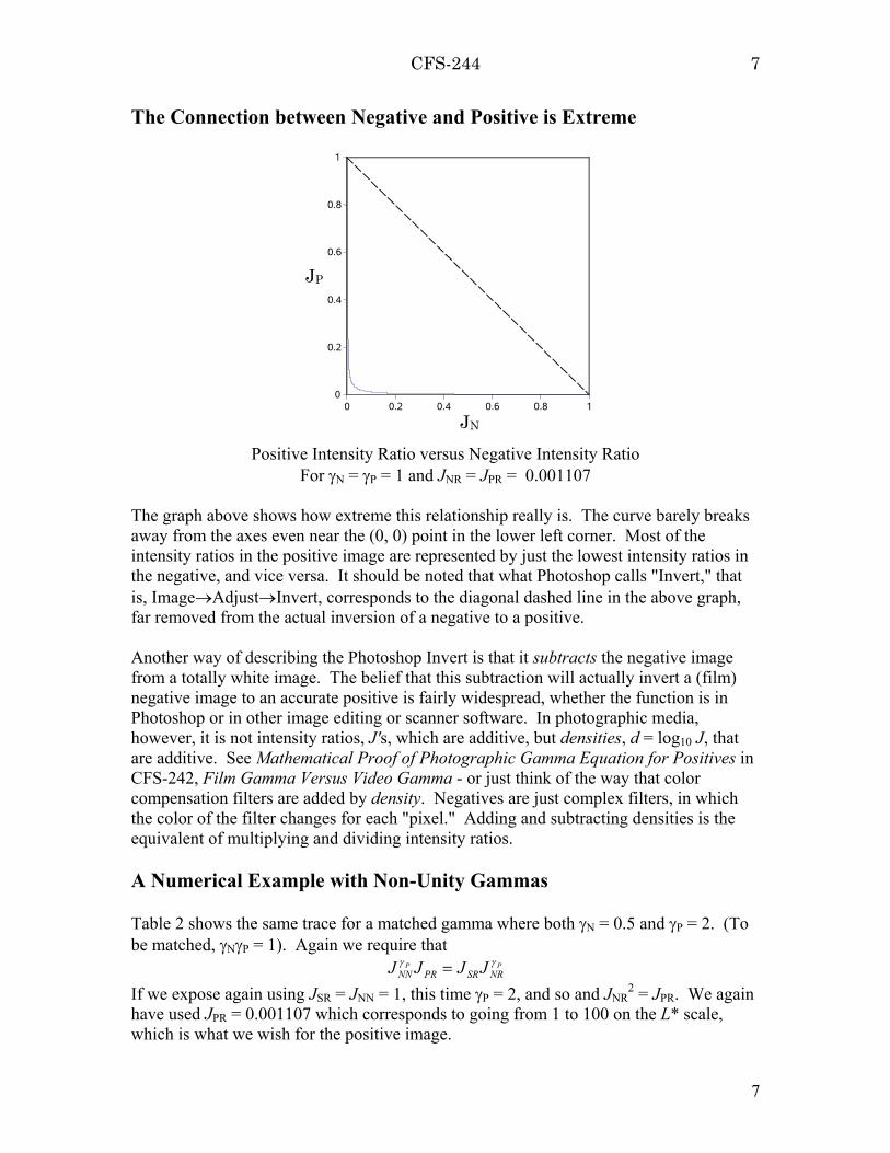
The Connection between Negative and Positive is Extreme

0 0.2 0.4 0.6 0.8 10

0.2

0.4

0.6

0.8

1

JP

JN

Positive Intensity Ratio versus Negative Intensity RatioFor γN = γP = 1 and JNR = JPR = 0.001107

The graph above shows how extreme this relationship really is. The curve barely breaksaway from the axes even near the (0, 0) point in the lower left corner. Most of theintensity ratios in the positive image are represented by just the lowest intensity ratios inthe negative, and vice versa. It should be noted that what Photoshop calls "Invert," thatis, Image→Adjust→Invert, corresponds to the diagonal dashed line in the above graph,far removed from the actual inversion of a negative to a positive.

Another way of describing the Photoshop Invert is that it subtracts the negative imagefrom a totally white image. The belief that this subtraction will actually invert a (film)negative image to an accurate positive is fairly widespread, whether the function is inPhotoshop or in other image editing or scanner software. In photographic media,however, it is not intensity ratios, J's, which are additive, but densities, d = log10 J, thatare additive. See Mathematical Proof of Photographic Gamma Equation for Positives inCFS-242, Film Gamma Versus Video Gamma - or just think of the way that colorcompensation filters are added by density. Negatives are just complex filters, in whichthe color of the filter changes for each "pixel." Adding and subtracting densities is theequivalent of multiplying and dividing intensity ratios.

A Numerical Example with Non-Unity Gammas

Table 2 shows the same trace for a matched gamma where both γN = 0.5 and γP = 2. (Tobe matched, γNγP = 1). Again we require that

PPNRSRPRNN JJJJ γγ =

If we expose again using JSR = JNN = 1, this time γP = 2, and so and JNR2 = JPR. We again

have used JPR = 0.001107 which corresponds to going from 1 to 100 on the L* scale,which is what we wish for the positive image.

CFS-244 8

8

Table 2 represents a thinner negative, that is, one with a lower dmax. If we allowed thenegative to be exposed to the same dmax as it was in Table 1, it would be possible to makea full-range positive image from a portion of the density range of the negative. Therewould still be (mathematically) an exact correspondence between the scene intensityratios and the positive image intensity ratios, at least for the range of ratios covered bythe positive image.

Table 2From Scene through Negative to Positive

For γN = 0.5, γP = 2 and JNR = 0.033272, JPR = 0.001107

LS* JS = [Y/Yn]S dN JN LN* dP JP = [Y/Yn]P LP*100 1 1.477916 0.033272 21.30949 0 1 100

96 0.900078 1.455056 0.035071 21.96989 0.045720 0.900078 9692 0.807044 1.431365 0.037037 22.66664 0.093103 0.807044 9288 0.720653 1.406779 0.039194 23.40321 0.142274 0.720653 8884 0.640658 1.381229 0.041569 24.18355 0.193374 0.640658 8480 0.566813 1.354636 0.044194 25.01217 0.246560 0.566813 8076 0.498872 1.326911 0.047107 25.89425 0.302010 0.498872 7672 0.436590 1.297953 0.050356 26.83581 0.359926 0.436590 7268 0.379720 1.267648 0.053995 27.84385 0.420536 0.379720 6864 0.328017 1.235864 0.058095 28.92658 0.484104 0.328017 6460 0.281233 1.202449 0.062741 30.09369 0.550933 0.281233 6056 0.239124 1.167228 0.068041 31.35677 0.621376 0.239124 5652 0.201443 1.129992 0.074132 32.72971 0.695847 0.201443 5248 0.167945 1.090499 0.081190 34.22944 0.774834 0.167945 4844 0.138382 1.048456 0.089443 35.87674 0.858920 0.138382 4440 0.112510 1.003511 0.099195 37.69753 0.948810 0.112510 4036 0.090082 0.955234 0.110858 39.72456 1.045364 0.090082 3632 0.070852 0.903091 0.125000 41.99996 1.149650 0.070852 3228 0.054574 0.846408 0.142427 44.57898 1.263016 0.054574 2824 0.041002 0.784319 0.164316 47.53577 1.387194 0.041002 2420 0.029891 0.715683 0.192450 50.97259 1.524466 0.029891 2016 0.020993 0.638954 0.229639 55.03515 1.677924 0.020993 1612 0.014064 0.551966 0.280565 59.93977 1.851900 0.014064 12

8 0.008856 0.451546 0.353553 66.02433 2.052740 0.008856 84 0.004428 0.301030 0.500000 76.06926 2.353772 0.004428 41 0.001107 0 1 100 2.955832 0.001107 1

0 0.2 0.4 0.6 0.8 10

0.2

0.4

0.6

0.8

1

JP

JN

Positive Intensity Ratio versus Negative Intensity RatioFor γN = 0.5, γP = 2 and JNR = 0.033272, JPR = 0.001107

CFS-244 9

9

The graph shows that the relationship between corresponding positive and negativeintensity ratios is still very extreme.

The practice of using a low-gamma negative has been widely used in manufacturingcolor negative films. Film (like most media) is largely limited by its dmax. Whennegative film is made with a low gamma (low contrast), the same dmax capability allows itto accurately represent a much wider range of scene intensity ratios, so that it has muchwider exposure latitude. When the negative is printed on media with a matched gamma(higher contrast), intensity ratios from the scene will be correctly represented, but ofcourse the positive print will represent only the range of intensity ratios that falls withinits dmax capability. A thin "underexposed" negative will print well but so will a dark"overexposed" negative. The quote marks are intended to mean that the negatives appearto be under- or over-exposed but are within the expanded latitude of the color negativefilm and so not actually under- or over-exposed.

Before we can effectively deal with real world inversion of negative to positive, we mustfirst deal with the much maligned "orange mask."

The Infamous Orange Mask

To judge from advice given on the web, it is widely believed that the problems in dealingwith color negatives are due mostly to the color mask, the pronounced orange, blue, orother color cast seen on most types of color negative. In actuality, the mask is equivalentto a uniform colored filter sandwiched with a negative color image that is more accuratethan could be obtained otherwise and more accurate than any positive color film. All thatis necessary to completely correct for the mask is to add a filter of complimentary colorto the mask.

Why the Orange Mask?

The colored dye molecules used to form images in color film are chemically combinedwith "coupler" molecules so that the combined molecule is colorless and transparent.When the film is developed, light exposed grains of silver halide are converted to silvermetal to form the image. Coupled dye molecules adjacent to the sites where silver grainsare formed break apart, releasing the dye molecule in its colored form, and the dyemolecules form the colored image. In color film the dyes are normally: magenta, whichpasses red and blue light freely but blocks green light; cyan, which passes green light andblue light freely but blocks red; and yellow, which passes red light and green light freelybut blocks blue. The problem is that very few types of dyes can be made to workchemically as required to form the coupled compounds that properly break apart duringfilm development. Consequently, the actual dyes that are used are not at all perfect. Forinstance, the magenta dye typically blocks some of the blue light it is supposed to passfreely, and the cyan typically blocks some of the blue and green light that it is supposedto pass freely.

CFS-244 10

10

A clever way of improving the dye action was introduced very early in color negativehistory. Instead of combining the dye molecules with coupler molecules that made themcolorless, the dye was combined with a coupler chosen so that the compound had exactlythe same light absorption as the unwanted absorption of the dye molecule. So, themagenta dye would be combined with a coupler producing a yellow-colored compoundso it would absorb some blue light just like the imperfect magenta dye, and the cyan dyewould be combined with a coupler producing a pinkish compound that would absorbsome blue and green light, just like the imperfect cyan dye. The pinkish and yellowcolors together formed the orange mask. If during film development some silver halidewas reduced to silver, causing a nearby magenta dye molecule to break loose of itscoupler, that meant the yellow coupled dye molecule had been broken and the yellow wasgone. So, throughout the image, either a magenta dye molecule would be present or theyellow coupled dye molecule remained. Either way, the same amount of blue light wouldbe absorbed, so the effect is like placing a yellow filter over a clear � but more perfect �negative. The same action with the cyan dye places a pinkish filter over the whole image.So, the entire mask effect is a filter that can be cancelled by adding a filtercomplimentary to the mask color - and brightening the image to compensate for thedarkening from the resulting "neutral density" filter.

Dealing with the Orange Mask

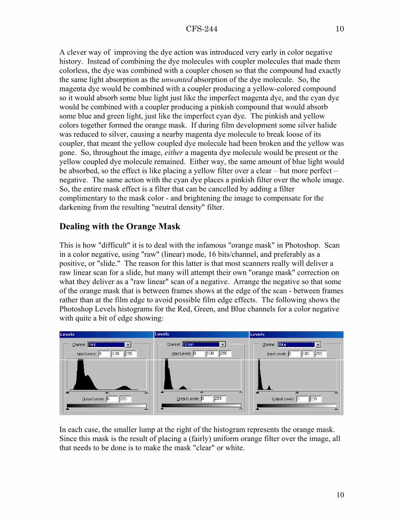
This is how "difficult" it is to deal with the infamous "orange mask" in Photoshop. Scanin a color negative, using "raw" (linear) mode, 16 bits/channel, and preferably as apositive, or "slide." The reason for this latter is that most scanners really will deliver araw linear scan for a slide, but many will attempt their own "orange mask" correction onwhat they deliver as a "raw linear" scan of a negative. Arrange the negative so that someof the orange mask that is between frames shows at the edge of the scan - between framesrather than at the film edge to avoid possible film edge effects. The following shows thePhotoshop Levels histograms for the Red, Green, and Blue channels for a color negativewith quite a bit of edge showing:

In each case, the smaller lump at the right of the histogram represents the orange mask.Since this mask is the result of placing a (fairly) uniform orange filter over the image, allthat needs to be done is to make the mask "clear" or white.

CFS-244 11

11

In the above illustration, at left is the Photoshop Levels showing RGB, and below thedialog box a small portion of the color negative image can be seen, with the orange maskat the edge. To correct the orange filter, we click the highlight button, the rightmosteyedropper1. Click on the orange mask and get a reasonably stable setting. The maskwill be mostly white, and the correction for the "orange mask" is completed. This is truewhether the orange mask really is orange, or if it is bluish, reddish, or some other color,as is the case for some varieties of color negative. Very easily done. The problems indealing with color negatives lie elsewhere. Incidentally, the "spiny" histogram on theright is due to the fact that Photoshop uses 8-Bits/Channel values for intermediatehistogram calculation even when the image is 16-Bits/Channel. The histogram of theimage is smooth when viewed after actual conversion, as shown below.

The result of removing the mask is shown below:

1 To use the highlight eyedropper properly, be certain this button is set to pure white, (R,G,B) =(255,255,255), which is the default value. This may be checked in the dialog box obtained by double-clicking the highlight button. Also, prior to calling the Levels tool, be certain that the eyedropper selectiontool is set to sample a 5x5 area rather than 3x3 or single point. This can be done by clicking the eyedropperin the "Tools" box and setting the "Sample Size:" The exact method varies with the version of Photoshop.Finally, prior to calling up the Levels tool it is wise to zoom in, select a portion of the edge and apply agaussian filter to it, enough to make it fairly uniform (typically 5 pixels or so), then deselect. Be sure theselected area is well within the uniform edge mask so that non-mask areas do not get blurred into thesample. Sample from this more thoroughly mixed area when correcting for the mask. With very grainynegatives this blurring becomes more necessary.

CFS-244 12

12

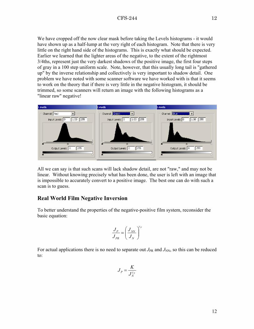
We have cropped off the now clear mask before taking the Levels histograms - it wouldhave shown up as a half-lump at the very right of each histogram. Note that there is verylittle on the right hand side of the histograms. This is exactly what should be expected.Earlier we learned that the lighter areas of the negative, to the extent of the rightmost3/4ths, represent just the very darkest shadows of the positive image, the first four stepsof gray in a 100 step uniform scale. Note, however, that this usually long tail is "gatheredup" by the inverse relationship and collectively is very important to shadow detail. Oneproblem we have noted with some scanner software we have worked with is that it seemsto work on the theory that if there is very little in the negative histogram, it should betrimmed, so some scanners will return an image with the following histograms as a"linear raw" negative!

All we can say is that such scans will lack shadow detail, are not "raw," and may not belinear. Without knowing precisely what has been done, the user is left with an image thatis impossible to accurately convert to a positive image. The best one can do with such ascan is to guess.

Real World Film Negative Inversion

To better understand the properties of the negative-positive film system, reconsider thebasic equation:

P

N

NN

PR

P

JJ

JJ

γ

=

For actual applications there is no need to separate out JPR and JNN, so this can be reducedto:

PN

P JKJ γ=

CFS-244 13

13

This inverse relationship has a very interesting property relative to the action of filters.Suppose we have a negative which has a histogram like the following:

There appears to be nothing on the right hand side of this histogram, so let us move overthe right hand Highlights slider until it meets the data. As we have learned previously,the Highlights slider is equivalent to a filter and/or a change in overall illumination andmerely multiplies all the JN's by a constant factor. Moving that slider is exactly whathappened above to the individual color channels to remove the orange mask filter. Thus,the action of moving the highlights slider is exactly the same as changing K in the aboveequation. Now consider the situation where we are looking at the histogram of a positiveimage, intending to move the highlights slider to apply a filter and/or a change in overallillumination. This will multiply all the JP's by a constant factor. So again the action ofmoving the highlights slider is to change the K in the above equation. Whether we areworking with the negative or the positive image, the action of moving the highlightsslider is to change K, so filters can be applied to either the positive or the negative as isconvenient for the required numerical operations.

Now we are equipped to experiment with a real photographic negative in Photoshop. Theimage for this experiment should contain a gray scale and the same gray scale should beavailable for direct comparison. For the purpose of illustration, we used a very old testnegative which included the image of a Kodak test booklet which we still have:

We scanned the negative as a slide in raw mode using a Minolta Dimage Scan Multi PROfilm scanner and removed the orange mask as described above. We then used thePhotoshop Curves tool to adjust the negative to match the positive. This was done usinga visual comparison with the gray scale in the original book and also numerically againsta positive scan of the book produced by a Hewlett Packard Scanjet 4670 flatbed scanner.The two methods produced very similar correction curves and the comparison with thescanned image is shown below:

CFS-244 14

14

This curve was determined using a PC computer which has an operating display gammaof 2.2. That is, what is stored as the computer image is "gamma adjusted"

c

PN

P JKJ

γ

γ

=* where γc = 0.45. The real Jp = [ ] c

PJ γ1* . Correcting the above curve for this

gamma gives a curve that looks like:

JP

JN

This curve can be closely matched with γP = 2.0 and K = 0.0085. Table 3 belowrepresents this real negative to positive inversion in the same format that we used above,going from scene to negative to positive.

CFS-244 15

15

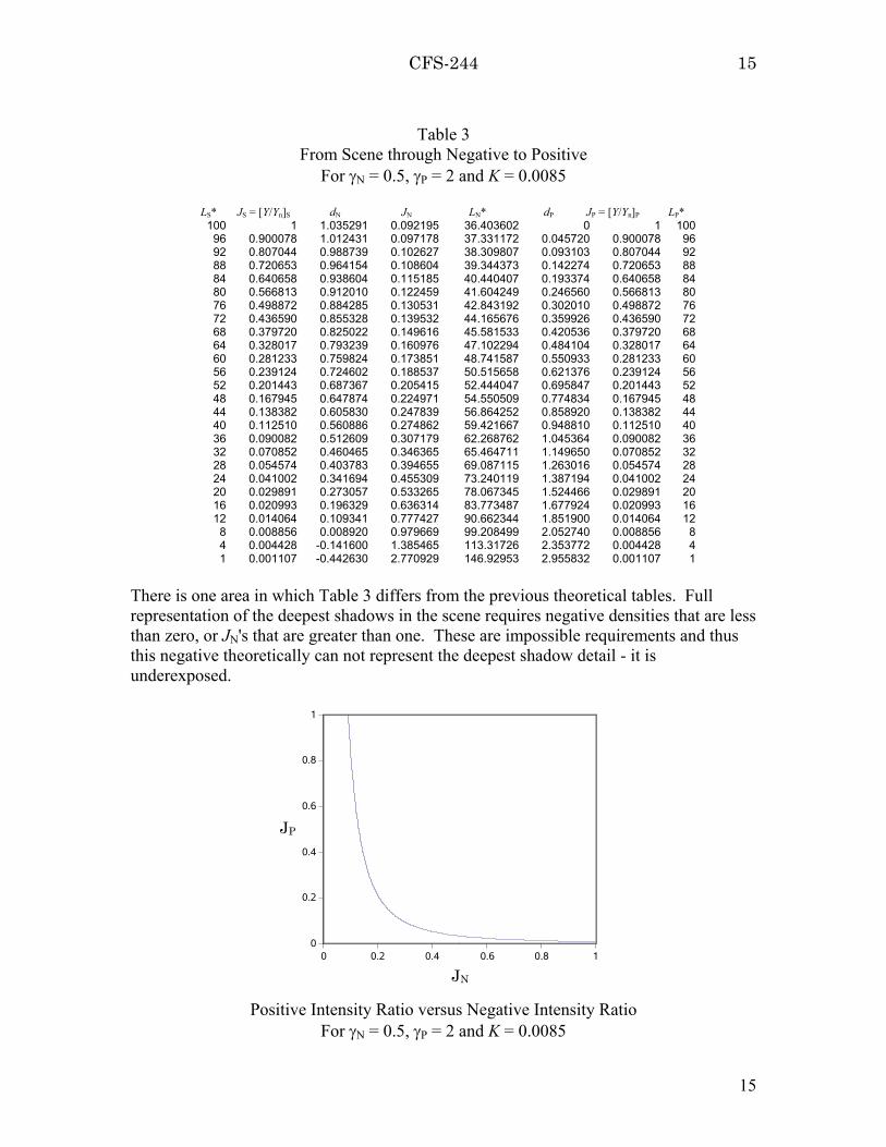
Table 3From Scene through Negative to Positive

For γN = 0.5, γP = 2 and K = 0.0085

LS* JS = [Y/Yn]S dN JN LN* dP JP = [Y/Yn]P LP*100 1 1.035291 0.092195 36.403602 0 1 100

96 0.900078 1.012431 0.097178 37.331172 0.045720 0.900078 9692 0.807044 0.988739 0.102627 38.309807 0.093103 0.807044 9288 0.720653 0.964154 0.108604 39.344373 0.142274 0.720653 8884 0.640658 0.938604 0.115185 40.440407 0.193374 0.640658 8480 0.566813 0.912010 0.122459 41.604249 0.246560 0.566813 8076 0.498872 0.884285 0.130531 42.843192 0.302010 0.498872 7672 0.436590 0.855328 0.139532 44.165676 0.359926 0.436590 7268 0.379720 0.825022 0.149616 45.581533 0.420536 0.379720 6864 0.328017 0.793239 0.160976 47.102294 0.484104 0.328017 6460 0.281233 0.759824 0.173851 48.741587 0.550933 0.281233 6056 0.239124 0.724602 0.188537 50.515658 0.621376 0.239124 5652 0.201443 0.687367 0.205415 52.444047 0.695847 0.201443 5248 0.167945 0.647874 0.224971 54.550509 0.774834 0.167945 4844 0.138382 0.605830 0.247839 56.864252 0.858920 0.138382 4440 0.112510 0.560886 0.274862 59.421667 0.948810 0.112510 4036 0.090082 0.512609 0.307179 62.268762 1.045364 0.090082 3632 0.070852 0.460465 0.346365 65.464711 1.149650 0.070852 3228 0.054574 0.403783 0.394655 69.087115 1.263016 0.054574 2824 0.041002 0.341694 0.455309 73.240119 1.387194 0.041002 2420 0.029891 0.273057 0.533265 78.067345 1.524466 0.029891 2016 0.020993 0.196329 0.636314 83.773487 1.677924 0.020993 1612 0.014064 0.109341 0.777427 90.662344 1.851900 0.014064 12

8 0.008856 0.008920 0.979669 99.208499 2.052740 0.008856 84 0.004428 -0.141600 1.385465 113.31726 2.353772 0.004428 41 0.001107 -0.442630 2.770929 146.92953 2.955832 0.001107 1

There is one area in which Table 3 differs from the previous theoretical tables. Fullrepresentation of the deepest shadows in the scene requires negative densities that are lessthan zero, or JN's that are greater than one. These are impossible requirements and thusthis negative theoretically can not represent the deepest shadow detail - it isunderexposed.

0 0.2 0.4 0.6 0.8 10

0.2

0.4

0.6

0.8

1

JP

JN

Positive Intensity Ratio versus Negative Intensity RatioFor γN = 0.5, γP = 2 and K = 0.0085

CFS-244 16

16

These tests above were done measuring and judging a gray scale in general. It ispossible, of course, to do the same thing to the individual primaries, red, green, and blue,finding a separate value of γP and K for each. In fact, there sometimes is an intentionalmanufacturing difference in the γP's for each color. This can be measured if there aregray scale images for the particular film type, and it can be visually estimated if severalnegatives of the film type are available for test, and it is found that, for example, theshadows run too blue in all of them while the highlights run too yellow. The K valueswill naturally tend to differ for the three colors, as the relative adjustment of the K's is theadjustment of overall color balance.

The Limits on K

The above example shows that there are limits on the value of K. When K is outsidethese limits the negative image is either under- or overexposed and the resulting positiveimage will lack either shadow or highlight detail. These limits depend upon dPmax, themaximum density range expressible in the positive image, and dNmax, the maximumdensity range of which the negative material is capable.

The operating relationship is:

PN

P JKJ γ=

To represent the complete density range of the positive image, at one limit the minimumexpressible JPmin = 10−dpmax will correspond to a density in the negative of zero, or JN = 1.Thus:

max10minmaxPd

PJK −==

At the other extreme, the positive density of zero, or JP = 1, must occur at or above anegative density JNmin = 10−dnmax, so:

pNJ

Kγ

min

min1 =

max10minminNpp d

NJK γγ −==

So for full range coverage

maxmax 1010 minminPpNp d

PNd JKJ −− =≤≤= γγ

Note that if γP = 1 and dPmax = dNmax there is only one value of K that works to give fullrange coverage. Normally γP > 1, and enough greater than one that even though typicallydPmax > dNmax, there remains a substantial range of values over which K can range and still

CFS-244 17

17

give full dynamic range coverage. For example, with γP = 2, if we assume that dPmax =dNmax = 3, the approximate range represented by the CIE L* "lightness" function themimics the behavior of the human eye, we find that the range is:

001.0000001.0 ≤≤ K

which is a substantial range of values.

For some additional perspective on this, the K for both Table 1 and Table 2 was0.001107, the high end of the range. In those tables the assumed dNmax was 2.95, justslightly shy of the 3 assumed in the above paragraph.

Digital Limitations on K

The negative to positive conversion involves taking a power, taking an inverse of that,and then taking that result to a power. While such operations are trivial and quite preciseon the double precision floating point digital arithmetic commonly used on computers,these same operations are problematical when using fixed point arithmetic of fairly lowprecision, as is commonly the case in working with digital images. Some problemsremain even if the actual calculations are done precisely and the low precision fixed pointis used only for image storage.

The complete transformation between negative and positive images is:

c

PN

P JKJ

γ

γ

=*

where γc, the "gamma adjustment," is usually 0.45 for PCs and 0.56 for Macs. Whenworking with negatives, the J 's are typically stored in 16-bit unsigned integers, thuslimited to integer values between 0 and 216 − 1 (= 65535), where the integer isunderstood to be divided by 65535 to obtain J. Eventually, the J's are usually convertedto 8-bit integers, limited to values between 0 and 28 − 1 (= 255) where the integer isunderstood to be divided by 255 to obtain J. Two different problems can occur, forvalues near JP* = 1 and for values near JP* = 0. For the purposes here we will define j asthe integer part of 65535 J.

First, near JP* = 1 (jP* = 65535) the possible values thin out. That is, two successiveinteger values jN and jN + 1 will produce widely spaced values jP* and jP* − m. Toproduce an image without visible "stair steps" in its tonal range, it is desirable that m ≤256 so that in the 8-bit version of JP*, all values 0 to 255 will be possible. To determinethis, start with

c

PN

P JKJ

γ

γ

=*

CFS-244 18

18

pccNP JKJ γγγ −=*

The problem will occur where JP* = 1:

pccNJK γγγ −=1

PKJ Nγ

1=

Find the rate of change in JP* with respect to JN:

1*

−−−= pccNPc

N

P JKdJdJ γγγγγ

substitute the value of JN where JP* = 1, and the absolute value of that derivative must beless than 256; that is, 1 step in 65535 for JN must lead to no more than 1 step in 255 inJP* (which is 256 steps in 65535 in JP*):

pp

pcc

KK PcPcγγ

γγγ

γγγγ11

256−

−−+

=>

pKPc

γ

γγ

1256 −

>

pKPc

γ

γγ

11256

<

−

p

Pc

Kγ

γγ

−

>

256

For the values used above, γP = 2 and γc = 0.45, this gives K > 0.0000124, so that theremight be stair-stepping in the highlights for a conversion toward the lower end of therange of K we gave for γP = 2 example above. This situation should be rare, but mightoccur for a very heavy negative. There appears to be no generalized remedy when it doesoccur (beyond dithering, which should be a last resort).

Shadow Treatment, Low JP*

The second problem occurs near JP* = 0 (jP* = 0), where high values of JN cannotpossibly produce the lowest values of JP*.

c

PN

P JKJ

γ

γ

=*

CFS-244 19

19

The highest possible value of JN is 1, so

cKJ Pγ=*

min

Obviously, that cannot be zero and to have j*Pmin = 1 (or J*Pmin = 1/65535) would requirethat for the example K = (1/65535)2.2 = 2.5×10-11, which is way out of the practical range.For practical purposes, as above, it would be desirable to have j*Pmin = 257 (or J*Pmin =1/255). Then K = (1/255)2.2 = 0.000005, which is still so low that it excludes most of thepractical range for the example case. In fact, we find that at the upper end of the range inthe example case K = 0.001 which leads to J*Pmin = 11/255, so that there can be no detailin the deep shadows represented by the first 10 counts in the 0 - 255 range of an 8-bitimage with a conversion K that large. In our underexposed test case, we found that K =0.0085, which leads to J*Pmin = 30/255, even worse.

This can present a serious problem, sometimes making it impossible to get deep shadowsfrom a negative. It should be pointed out in passing that most of this problem is due tothe "gamma correction," that is, c

PP JJ γ=* . In CFS-243, Maintaining Color Integrity inDigital Photography we mentioned that the "Levels" gamma correction in Photoshop isincorrect for gammas around the value of γc = 0.45 (or 2.2 in Photoshop convention), andwe believe this error is really intended to be a makeshift correction for the problem weare dealing with here.

While there is no completely accurate solution to this problem when it occurs, there is apractical work-around. For the work-around, we will adjust JP instead of JP* in order tolessen the distortion of the colors in the shadows. This color distortion effect is explainedfully in CFS-243.

We can adjust JP so that the minimum will be zero:

c

P

PPPadj J

JJJγ

−−

=min

min*

1

Note that to use this form we must use JPmin instead of J*Pmin in order to properly matchJP. Thus if we choose to take JPmin where JN = 1, then JPmin = K. In practical terms, itoften makes more sense to find from histogram data the JNmax as the largest value forwhich there is a significant count of pixels. (Alternatively, above which the count ofpixels is small enough to be ignored.) In doing this, it is well to remember that in thislightest area of the negative, a long range of brightnesses will represent just a short rangeof brightnesses in the darkest shadows of the positive, so a long span of nearly emptyhistogram cells is important to the shadow quality of the result. In any event, therelationship then becomes:

PN

P JKJ γ

maxmin =

CFS-244 20

20

The key to the success of this operation is to perform all the intermediate calculations infull double precision floating point arithmetic on the computer and never store anintermediate integer value of jP. That is, to perform the calculation as:

c

P

PP

N

NNPadj

JKJ

KJK

J

γ

γ

γγ

−

−=

max

max*

1

Note that in terms of computer operations, once K, γP , γc, and JNmax are known, a tablecorresponding to all 65536 possible values of JN can be formed and filled with the doubleprecision computed values of J*Padj, so that the actual conversion of an image file can bedone using the resulting lookup table.

Alternatively, an adjustment can be made that may be more accurate in terms of colorintegrity (although preliminary testing suggests that the changes in color would beessentially invisible in most cases). First, for the largest component, "m" of R, G, B, (thatis, the smallest JNq where "q" is the color index) calculate:

−

−=

P

PP

Nm

NmNmPadj

JKJ

KJK

Jγ

γγ

max

max

1

Note that this is not gamma adjusted. Then, also calculate the uncorrected values foreach component:

PNq

Pq JKJ γ=

Note that although substitution tables are no longer possible, a set of four tables of doubleprecision calculated values can be created and used. So, for the predominant primary m,and for color q, use:

c

Pm

PqPadjPq J

JJJ

γ

=*

This calculation preserves the ratios between the color components as they should be inthe linear positive image, and thus is more accurate but slower to calculate. The entirecalculation should be kept in double precision floating point until J*P for the final imageis stored.

CFS-244 21

21

Highlight Treatment, Low JN

On most of the JP versus JN curves we have shown, at low JN, there is a considerable gapbetween the curve and the axis even when it reaches JP = 1. It appears like this gap mightrepresent considerable loss in highlight detail, but that is mostly an illusion. This area ofthe curve is where the negative is at its greatest density, and that will normally not befull-scale of the scanner. Thus no pixels will have intensities for the lowest JN values,and the "missing" values will not be a problem at all. The best approach is to find JNminfrom histogram data, the lowest JN for which there is a significant pixel count. The valueof K can then be set to that JP = 1 at this JN.

PNJK γ

min=This is the best starting value of K, and the minimum value which will retain all theshadow detail.

Final Summary

The infamous "orange mask" that is so often blamed as the main source of difficulty indealing with film negatives is actually very easily handled.

The relationship between the positive and negative images is an inverse one:

c

PN

P JKJ

γ

γ

=*

Here γc is the "gamma adjustment" that is typically applied to images stored in PCs, andthe star notation means that the positive image J*P has been gamma adjusted. The realproblem in dealing with negatives is in determining γP and K. γP should be nearly thesame for all properly processed color negatives of a particular film type, although γP maybe different for each of the three primary colors. It can be visually estimated byexamining test images of a negative inverted to a positive, particularly if several tests aremade and compared, but is more accurately estimated by comparison of an invertedimage to a known final image. The correct estimation of γP is important to image colorintegrity, since this γP should be "matched" to the γN of the negative to get the colorscorrect.

The K regulates the overall lightness/darkness of the image. The best estimation orselection of K varies from negative to negative, even of the same negative type. Colornegatives typically are designed with γN < 1, which gives them wider exposure latitude,and K is a measure of exposure. A starting value for K is P

NJK γmin= , and there are

numerous constraints, adjustments, and calculation methods for K that arise fromphysical and numerical considerations.

CFS-244 22

22

Since color negatives have a wide latitude, it will sometimes be that case that finalpositive images are best made as composites of two images derived using different Kvalues. An example would be a landscape in which the sky is bright enough to lackdetail. The second image would be darker, showing the sky detail. This is similar to thetraditional photographic technique of "burning in" the sky working with a color negativeand an enlarger. Much more detail is potentially available than would be available fromdigitally burning in the image from a single K conversion.

For best results, separate values of γP should be obtained for each of red, blue, and green,for a particular film type, estimated from gray scale images if possible. Differinggammas for the separate colors can be visually estimated if several negatives of the filmtype are available for test, and it is found that, for example, the shadows run too blue inall of them while the highlights run too yellow. The K values for the three primaries willnaturally tend to differ for the three colors, as the relative adjustment of the K's is theadjustment of color balance.

The method of conversion of negative to positive that is described here, including the useof the correct gammas, is necessary to preserve the color integrity of the original negative(see CFS-243, Maintaining Color Integrity in Digital Photography for further elaborationof this problem). The result may have a tonal scale that needs improvement; often it willbe too dark. A "curves" adjustment in 16-Bits/Channel mode could compress thehighlights without losing detail. Since at this point the colors should be correct or atworst out of color balance in a way that can be adjusted by a color correction filter, thebest method is to convert the image to CIE Lab color and adjust the Lightness curve inthat mode to place the tonal values where they are wanted. The image can then beconverted back to RGB for further adjustment, including final color balance.