Near-Real-Time Monitoring of Small Reservoirs with Remote Sensing

Small Reservoirs Toolkit

1 1

Near‐Real‐Time Monitoring of Small Reservoirs with Remote Sensing

Authors Jens Liebe, Center for Development Research, University of Bonn, Germany Nick van de Giesen, Delft University of Technology, the Netherlands Frank Ohene Annor, Kwame Nkrumah University of Science and Technology, Kumasi, Ghana

Scope: questions/ challenges the tool addresses This tool focuses on the use of radar satellite images to monitor changes in small reservoir surface area. Surface area can be translated into storage volume on the basis of regional bathymetric surveys. Because radar is not affected by clouds, a near-real time record of water stored in small reservoirs can be produced every two to four weeks. Such records are of interest to hydrologists and are useful in drought monitoring.

This tool is different from the Reservoirs Inventory Mapping Tool in that it uses radar satellite images, not optical imagery. Optical imagery can be problematic when there is cloud cover. Further development is needed to automate reservoir delineation in radar images to facilitate large scale application.

Target group of the tool On the basis of the information provided here, along with the referenced literature, a technically schooled person with an introductory knowledge of remote sensing should be able to produce, every two to four weeks, estimates of reservoir surface area. Such estimates are of direct interest to water managers and planners working at regional/provincial, national, or sub-continental scales of analysis.

Patience and perseverance are required because the tool involves the interpretation of radar images. There are a number of good on-line introductory remote sensing tutorials, including:

http://ccrs.nrcan.gc.ca/resource/tutor/fundam/index_e.php

http://rst.gsfc.nasa.gov/Front/overview.html

Requirements for tool application Access to remote sensing software, radar images, reasonably fast computers, and ample digital storage space are prerequisites. Internet access is also helpful. The methods described are based on radar images obtained through Envisat of the European Space Agency (ESA). For obtaining Envisat images, see eopi.esa.int. ESA's Tiger project may also be of interest (www.tiger.esa.int ). Other sources of radar images are the Canadian Radarsat and the Japanese ALOS.

Small Reservoirs Tool Kit

2

Tool: description and application Classification with radar satellites

Measuring small reservoir surface area is a matter of distinguishing open water from dry areas. This can be done easily with optical imagery as long as there are not too many clouds. In the wet season, however, semi-arid areas are covered with clouds most of the time. An alternative approach is to use radar imagery because radar penetrates cloud cover.

A radar satellite is an active instrument. The satellite sends out a short pulse and measures the reflected energy, called “backscatter”. By timing the return, the distance from the satellite can be calculated and an image can be built up. Different radar bands are used that correspond to different wavelengths in the microwave part of the electro-magnetic spectrum, such as C-band (5 cm, i.e. Envisat and Radarsat), and L-band (20 cm, i.e. ALOS).

Apart from wavelength, polarization is also important. Envisat, for example, can send out pulses with horizontal (H) or vertical (V) polarization and can also measure returned pulses as H or V. In this study, use was mainly made of Envisat dual-polarization images consisting of two bands, one HH (horizontal out, horizontal in) and one HV (horizontal out, vertical in). When there are no complicating factors, open water stands out clearly from darker surrounding vegetated areas, as seen in Figure 1.

Figure 1: Sample Envisat HH image with two small reservoirs (A), an irrigated area (B), and a village (C). The remainder consists of sparse trees with dried grasses and crops residues

Sometimes, however, there are complicating factors. In theory, most of the energy sent by the satellite in the form of a radio pulse should be reflected away from the satellite by the relatively


3

smooth water surface. The surrounding rough and vegetated areas should reflect much more energy back to the satellite. In practice, things are not this simple. Problems discussed here include the effect of floating vegetation in reservoir tails, wind-induced backscatter (Bragg scattering), and lack of backscatter from surrounding dry areas.

Usually, some spatial filtering of the original images is needed. Different filters are available, but the adaptive gamma-map filter and the Lee-filter seemed to give the best results in general. These filters move a small window of 3x3, 5x5, or 7x7 pixels over the image and assign a value to the center pixel based on the values of the pixels in the window. This can simply be the average, which gives a smoothened image that is easier to interpret, but also has blurred edges. Adaptive filters, like the ones used, look at the statistics within the window and maintain sharp transitions better.

After filtering, simple density slicing, followed by a contiguity operation, gives good reservoir outlines. Annor (2007) was able to explain 90% of the variation in surface area observed on the ground on the basis of Envisat images. A detailed description of the necessary steps is given in Annex 1.

Floating vegetation causes problems for both optical and radar satellites. It is often difficult to distinguish between floating vegetation (in the reservoir) and well-watered wetland vegetation (outside of the reservoir). Even in the field, the distinction is at times somewhat arbitrary because such vegetation tends to be concentrated in or near the shallow tail end of reservoirs. The use of L-band radar imagery (ALOS) seems most suitable: this imagery is better at penetrating floating vegetation due to its greater wavelength. However, the use of ALOS for


4

this purpose is at an early stage. For other satellites, floating vegetation is basically indistinguishable from the surroundings. Fortunately, the amount of water stored in these shallow areas tends to be minimal. During bathymetric surveys, floating vegetation should be clearly delineated. The effect of floating vegetation is discussed in detail in Annor (2007).

Wind causes ripples on the reservoir surface, sometimes resulting in significant backscatter to the satellite, so-called Bragg scatter. Instead of appearing dark, water appears light, often as bright as, or even brighter than, surrounding dry areas. A first precaution is to use images that are acquired during the evening overpass when wind tends to be significantly less than during the day. During some periods, however, winds are stronger and last longer (for example, at the onset of the rainy season). At these times, Bragg scatter may make it difficult to estimate reservoir surface area. The use of dual-polarization images then becomes important. Often, if Bragg scatter occurs in, say, the HH band, it will not occur in the HV band. In general, the HV band is less subject to Bragg scatter, but gives, in cases without Bragg scatter, a water-land contrast that is less pronounced than HH.

Figure 2: ASAR Images of a small reservoir. With (right) and without (left) Bragg scatter induced by wind (indicated). Yellow arrow depicts look direction

It is not yet possible to automatically classify radar images affected by Bragg scatter. Rather, manual analysis is needed. Patches that clearly belong to the reservoir are first selected. These patches are then “grown” to absorb all adjacent pixels that fall within a certain number of standard deviations from the sample. The allowable spread can only be determined interactively, which makes classification a labor-intensive process. Even then, some images (typically around 10%) cannot be classified reliably. This is especially the case at the end of the dry season when areas surrounding the reservoir have become so dry that backscatter from land becomes as low as that from open water.

A systematic overview of these problems can be found in Liebe et al. 2008. Most radar images used were acquired through the ESA Tiger initiative, project #2871, see: http://tiger2871.shorturl.com for more information.

Lessons learned Although the use of radar imagery for identifying open water is supposed to be relatively straightforward, in practice it turned out to be rather difficult. Over the course of a year, radar images were most likely to be affected by wind during the onset of the rainy season (in Ghana, during May and June). Because of lower wind speeds and reduced Bragg scatter, night-time


5

radar image acquisitions were generally preferred. Based on a 15 month wind speed prevalence analysis conducted at a reservoir in the Upper East Region of Ghana, we found that wind speeds were too low to produce Bragg scatter in 96% of night-time acquisitions, compared to 50% for morning acquisitions. Night time acquisition of radar images is therefore recommended (Liebe et al. 2008).

We conclude that radar and optical systems are complementary for monitoring reservoir surface area. Optical systems yield good results during the dry season, but are affected by excessive cloud cover during the rainy season. Radar is unaffected by cloud cover, but is affected by wind (Bragg scatter) and lack of vegetation contrast during the dry season.

Recommendations The application of radar imagery for operational purposes requires (a) smarter algorithms to automate the delineation of individual reservoirs or (b) the dedicated time of a skilled remote sensing specialist. Until automated algorithms are developed, this tool is most appropriate for obtaining insights into the filling (and emptying) of reservoirs in a limited area of interest over one or two hydrological cycles. Only when the process is automated can it be used for more rigorous hydrological research and drought monitoring

Limitations of the tool The application of radar imagery for operational purposes still requires either smarter algorithms to automate the delineation of individual reservoirs or the dedicated time of a skilled remote sensing specialist.

References Annor 2007: Delineation of small reservoirs using radar imagery in a semi-arid environment: A case

study in the Upper East Region of Ghana, Master thesis, UNESCO IHE, Delft, Netherlands (http://www.smallreservoirs.org/full/publications/reports/Annor_FO.pdf).

Liebe, J., M. Andreini, N. van de Giesen, M. T. Walter, and T. Steenhuis, 2009. Suitability and limitations of ENVISAT ASAR for monitoring small reservoirs in a semi-arid area. IEEE Transactions on Geosciences and Remote Sensing 47(5): 1536-1547.

Liebe 2002: Estimation of Water Storage Capacity and Evaporation Losses of Small Reservoirs in the Upper East Region of Ghana. Diploma thesis, University of Bonn, September 2002. (http://www.glowa-volta.de/publications/printed/thesis_liebe.pdf)

Liebe et al 2005: Estimation of Small Reservoir Storage Capacities in a semi-arid environment. A case study in the Upper East Region of Ghana. J. Liebe, N. van de Giesen, M. Andreini. Physics and Chemistry of the Earth, 30: 448–454, 2005 (doi:10.1016/j.pce.2005.06.011, http://dx.doi.org/10.1016/j.pce.2005.06.011).

Liebe et al 2008: Monitoring small reservoirs’ extent and volume in a semi-arid area with ENVISAT ASAR.

Sawunyama et al 2006: Estimation of small reservoir storage capacities in Limpopo River Basin using GIS procedures and remotely sensed surface areas – Case Study of Mzingwane Catchment, Zimbabwe. T.


6

SAWUNYAMA, A. SENZANJE and A. MHIZHA, 2006, Physics and Chemistry of the Earth. Vol.31, Issues 15-16:935 – 943. http://dx.doi.org/10.1016/j.pce.2006.08.026

Tiger project AO2871: http://tiger2871.shorturl.com

Contacts and Links Jens Liebe, Center for Development Research, University of Bonn, Germany: jliebe@uni-

bonn.de Nick van de Giesen, Technical University of Delft, The Netherlands,

[email protected] Frank Annor, Kwame Nkrumah University of Science and Technology, Kumasi, Ghana,

[email protected], Remote sensing tutorials http://ccrs.nrcan.gc.ca/resource/tutor/fundam/index_e.php http://rst.gsfc.nasa.gov/Front/overview.html Free remote sensing software http://www.itc.nl/ilwis/ Radar data sources http://eopi.esa.int


7

Annex 1

TRAINING MANUAL FOR MONITORING WATER STORAGE IN SMALL RESERVOIRS BY REMOTE SENSING

Prepared by Frank Ohene Annor

Nick Van de Giesen & Jens Liebe

February, 2007


8

How to process ENVISAT‐ASAR Alternating Polarization (dual) mode data to delineate the outlines of reservoirs using Erdas Imagine9.1 and ArcGIS9.2

3. REDUCE SPECKLES BY USING GAMMA-ADAPTIVE FILTER IN ERDAS

RADAR MODULE (7X7 WINDOW )

1. ENVISAT-ASAR ASA_APS DATA

4. REDUCE SPECKLES BY USING GAMMA-ADAPTIVE FILTER IN ERDAS

RADAR MODULE (5X5 WINDOW)

2. IMPORT INTO ERDAS IMAGINE USING A LINEAR TRANSFORMATION

OF 1

5. GEOCODE USING UTM COORDINATES ( FOR UER, IT IS ZONE

30N) ON THE WGS84 ELLIPSOID IN ARCMAP

GO TO STEP 8

6. PERFORM AN UNSUPERVISED CLASSIFICATION IN THE CLASSIFIER

MODULE IN ERDAS IMAGINE. IF SATISFIED WITH THE RESULTS GO

TO STEP 9, ELSE GO STEP 7

7. EDIT THE SIGNATURE OBTAINED IN THE UNSUPERVISED

CLASSIFICATION IN THE ERDAS CLASSIFIER MODULE USING ONE OR

SAMPLE SAMPLE SITE(S) TO CLASSIFIER AREAS/OBJECTES OF

INTEREST


9

Use the screen shots below as a guide for all the steps!

9. ADD THE CLASSIFIED IMAGE AS A

LAYER IN ARCMAP

8. PERFORM A SUPERVISED CLASSIFICATION IN THE ERDAS CLASSIFIER MODULE USING THE

EDITED SIGNATURE

11. CREATE A NEW SHAPEFILE (POLYGON) IN ARCCATALOG. THIS

WILL BE USED FOR THE OUTLINE OF THE RESERVOIRS

10. GEOREFERENCE THE IMAGE USING GCP POINTS EITHER FROM

FIELD WORK OR FROM A GEOREFERENCED MAP/IMAGE

USING A GREATLY OVER DEFINED 1st OR 2nd ORDER POLYNOMIAL (AFFINE) TRANSFORMATION IN

ARCMAP

12. ADD THE NEW SHAPEFILE TO THE DATA FRAME THAT CONTAINS THE

CLASSIFIED IMAGE AS A LAYER

13. PERFORM AN ONSCREEN DIGITIZATION TO DETERMINE THE AREA EXTENT OF THE RESERVOIRS

14. USE XTOOLSPRO4.1 OR CALCULATE GEOMETRY IN THE ATTRIBUTE TABLE OF THE NEW POLYGON TO CALCULATE THE

PERIMETER AND SURFACE AREA OF THE DIGITIZED RESERVOIRS


10

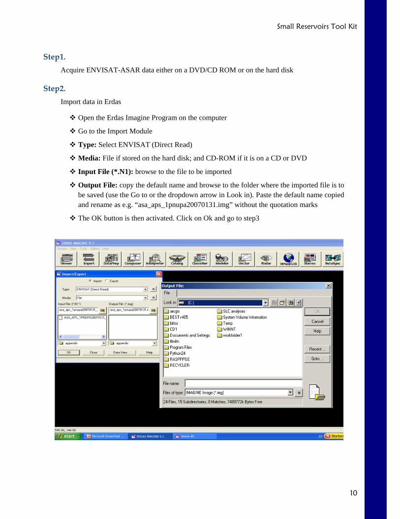
Step1. Acquire ENVISAT-ASAR data either on a DVD/CD ROM or on the hard disk

Step2. Import data in Erdas

Open the Erdas Imagine Program on the computer

Go to the Import Module

Type: Select ENVISAT (Direct Read)

Media: File if stored on the hard disk; and CD-ROM if it is on a CD or DVD

Input File (*.N1): browse to the file to be imported

Output File: copy the default name and browse to the folder where the imported file is to be saved (use the Go to or the dropdown arrow in Look in). Paste the default name copied and rename as e.g. “asa_aps_1pnupa20070131.img” without the quotation marks

The OK button is then activated. Click on Ok and go to step3


11

to use a transformation of 1

o Tick the “Write Transform to image and Write GCP File” box. For transformation Order, select 1. It is not so necessary to save the GCP file unless it is to be used for co-registration. Click on ok to start importing the file

o Click on ok (when the processing is completed, the OK button will be activated)


12

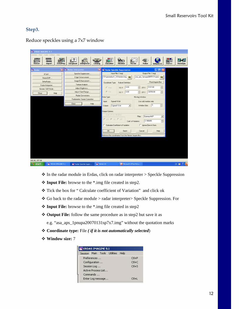
Step3.

Reduce speckles using a 7x7 window

In the radar module in Erdas, click on radar interpreter > Speckle Suppression

Input File: browse to the *.img file created in step2.

Tick the box for “ Calculate coefficient of Variation” and click ok

Go back to the radar module > radar interpreter> Speckle Suppression. For

Input File: browse to the *.img file created in step2

Output File: follow the same procedure as in step2 but save it as

e.g. “asa_aps_1pnupa20070131sp7x7.img” without the quotation marks

Coordinate type: File ( if it is not automatically selected)

Window size: 7


13

Filter: Gamma-map

Coef. of Variation: Go to session on the main menu bar > Session log , copy the coefficient of variation computed and paste it

Click ok to start filtering

Step4. Reduce speckles using a 5x5 window

Repeat step3 but choose 5 for Window size instead of 7 and name the file as

“asa_aps_1pnupa20070131sp5x5.img”

Step5. 5a. Geocode using UTM coordinates

Open the ArcMap program in ArcGIS9.2.

Click on add data tool

add asa_aps_1pnupa20070131sp5x5.img as a layer

Right click an empty space in the tools box, go to Environments > General settings and set the environments (i.e. where to save the files etc.)

In the tools box, click on data management tools > define projections


14

o input dataset or feature class : Use the drop down arrow to select the file asa-_aps_1pnupa20070131sp5x5.img or browse to the folder which contains this file

o coordinate system : Select Geographic coordinate systems\World\WGS 1984.prj and click on add, click on apply, ok and another ok

In the data management tools > click on projections and transformation > Raster > Project

o Input raster: asa_aps_1pnupa20070131sp5x5.img

o Output raster: e.g. 310107prj (it should be less than 10characters)

o Output coordinate System: Select projected coordinate system \UTM\WGS 1984\WGS 1984 UTM Zone 30N.prj (for Upper East Region of Ghana)

o Click on environments and ensure that under general settings, the output coordinate is set to “As specified below” and specify the coordinate system as the previous step (UTM)

o Click on ok to start the projection

Create a new map and add one of the bands of the projected data e.g. 310107_c1

Add one band of the projected data as a layer

5b. In order to change the format for the projected image from grid to *.img

Go to ArcTool box and click on Spatial Analyst Tools > Extraction > Extract by mask

For

o Input raster: use the drop down arrow and select the projected file e.g. 310107_c1 or browse to the file

o Input raster or feature mask data: Select the same file

o Output raster: save it under a name (less than 10 characters) followed by “.img” to get it into an imagine file format e.g. 310107_c1.img

o Check the Environments to be sure it has the right settings and click on ok

Step6. 6a. To maintain the format and perform an unsupervised classification in ArcGIS

Go to spatial Analyst Tools > Multivariate > Iso cluster

For

o Input raster bands: Add the three bands of the projected raster file *_c1, *_c2 and *_c3

o utput signature file: give it a suitable name e.g. sig310107 ( be mindful of where it is being saved since it will be needed for the classification)


15

o Number of classes: depends on how many land covers is to be classified e.g. 6 classes

o You can fill in the optional fields or use the default

o In the Multivariate tool > Maximum likelihood

Input raster bands: add the three bands again

Input signature file: the signature created in the Iso Cluster (e.g. sig310107)

Output classified raster: give it a name

Fill the other fields or use the default values

6b. To perform an unsupervised classification in Erdas Imagine

Go to the classifier module in Erdas imagine

click on unsupervised classification

For

o Input raster: use the output from step 5b.

o Output cluster Layer: give it a name and save it in the correct folder

o Out put signature Set: ditto

o Open the file in ArcMap and check which class has been assigned for water


16

Step7. To edit the signature obtained in the unsupervised classification in Erdas for a supervised classification

Go to the classifier module in Erdas

Click on Signature Editor

Go to file > open and browse to where the signature was saved during the unsupervised classification

Select the Replace option and click on ok

Go to the viewer module without closing the signature editor

Select the Classic viewer option

Browse to the file which was used for the unsupervised classification ( that is the output file from step 5b.) and open it

If prompted to build pyramid layers, select YES ( Imagine uses a 2x2 resampling algorithm by default)

Scroll both to the right and down to see the image or use the zoom out button to see the full image

Zoom-in to an area which can be identified as water


17

Go to file in the viewer module > New > AOI layer

Click on the show tool palette for Top layer ( the tool that looks like a hammer)

In the AOI tools select the ellipse to create and ellipsoidal area of interest in the area that is identified to be water

Go to the signature editor and highlight the class for water by clicking on the class number under Class #

On the menu bar in the signature editor click on replace current signature(s) with AOI

Step8. To perform a supervised classification in Erdas Imagine

Continue from step 7

Select all the classes in the signature editor by holding on to the shift key and clicking on the class names

Go to Classify in the signature editor menu bar and select supervised

For

o Output file: give it a name and save it to a folder

o If threshold is to be performed then tick the output distance file option and give it a name

o None parametric rule: None

o Parametric rule: Maximum Likelihood

o Click on OK to start the supervised classification


18

Step9. Add the classified image as a layer in ArcMap

Step10. To georeference the image using GCPs in ArcMap

Add the ground control points to the image in the form of a shapefile (points, polygon, polyline etc.) obtained from a GPS defining a particular area of interest or use intersections of roads or well known points as control points. e.g. In the figure below; the shaded one is the GCP and the coloured area is the classified image

On the menu bar, right click an empty space and click on Georeferencing to add it to the main menu bar

For layer: select the layer to be transformed/georeferenced

Click on add control points

Select a point in the image to be transformed by clicking on the point and move the curser to the correct position where it should be using the control points


19

Repeat this for as many points for which there are control points ( Avoid using points at the extreme ends

click on the “show links and error” button next t o the control points to show the XY positions and the transformed XY positions in tabular form

For transformation: Select 1st Order or 2nd order Polynomial (Affine) transformation

Check the Total RMS Error to determine whether the transformation is acceptable

Go to georefencing > Rectify

o Cell Size: leave the default unless there are multi-image processing which requires a particular cell size, then it can be changed

o Resample type: accept the default which is Nearest neighbour which is applicable to both discrete and continues data

o Output location: browse to the folder where the georeferenced image is to be saved

o Name: Give it an appropriate name

o Format: Imagine Image


20

Save the work

Add the georeferenced image as a layer in ArcMap

Step11. Create a new shapefile (polygon) in arccatalog. this will be used for the outline of the reservoirs

Step12. Add the new shapefile to the data frame that contains the classified image

Step13. Perform an onscreen digitization to determine the area extent of the reservoirs

Create a shapefile in Arccatalog

o Open the ArcCatalog program in ArcGIS or Click on the Arccatolog icon in ArcMap

o Right click an empty space in the extreme right pane


21

Create a shapefile in Arccatalog

o Go to New > Shapefile

o Name: give it a suitable name

o Feature type: Select polygon

o Spatial Reference: Click on edit > Select > Projected coordinate system > UTM > WGS 1984 > UTM Zone and click on “Add”


22

Add the shapefile as a layer in the data frame that contains the georeferenced image

Right click on an empty space on the main menu bar and select Editor > start editing > Select the shapefile to be edited if there are a number of them and click on OK

Go to editor > Start editing

Select the sketch tool

Mark the outline of a reservoir with the sketch tool

When done, click on editor > Save edit

Repeat this for all the reservoirs of interest

When done, click on editor > Save edit > stop editing


23

Step14. Calculate the area of the polygon created in step 13 using Xtools Pro or Calculate Geometry in ArcMap attribute table

Go to tools (or use Alt + T) > Extensions > select XtoolsPro (if that extension is available; a trial version can be downloaded at

http://www.xtoolspro.com/download.html)

In XTools Pro > Table Operations > calculate Area, Perimeter,Length...

o Select layer to measure: Select the shapefile created for the outlines of the reservoirs

o Desired output: Select the appropriate unit

o Check the parameters to be measured (e.g. Perimeter and Area) and click on OK

Open the attribute table of the shapefile to read the values of the parameters measured

If the Xtools extension is not available then follow the following steps to measure the parameters in ArcMap

Open the attribute table of the shapefile

Go to options > Add field

o Name: e.g. Area

o Type: Text ( choose an appropriate length like 50 or 100 characters) and click on OK


24

o Right click on the Area column > Calculate Geometry ( if prompted that the calculation is being done outside an edit session; Select YES)

o Select the appropriate units and click on OK

o Save the edits

o Stop editing when done

Save the work


25

How to import XYZ points from a GPS to Polygons in ArcGIS

1. CONNECT THE GPS TO YOUR COMPUTER VIA USB OR SERIAL PORT

2. OPEN THE GPS TRACKMAKER PROGRAM AND SELECT THE APPROPRIATE GPS INTERFACE IN THE GPS FUNCTION ON THE MENU BAR

3. SELECT THE CORRECT COMM PORT AND CLICK ON THE PRODUCT ID BUTTON TO RETRIEVE THE STORED ROUTES, TRACKLOGS AND WAYPOINTS

4. DOUBLE CLICK ON WAYPOINTS, GO TO TOOLS ON THE MENU BAR AND SELECT OPTIONS UNDER TOOLS. CLICK ON COORDINATES AND SELECT THE CORRECT ONE (RECTANGULAR GRIDS, UTM FOR UER)

5. SAVE THE FILE AS BOTH GPS TRACKMAKER FILE (*.gtm) AND TEXT FILE (*.txt)

6. OPEN THE TEXT FILE IN MICROSOFT EXCEL. FOR FILE TYPE, CHOOSE TEXT. OPEN THE TEXT FILE WHICH WAS SAVED IN GPS TRACKMAKER. CHOOSE DELIMITED FOR DATA TYPE. CLICK ON NEXT. FOR DELIMETERS, CHOOSE COMMA. CLICK ON NEXT. FOR COLUMN DATA, CHOOSE GENERAL

7. DELETE ROWS 1 TO 4. MAKE SURE THAT THE DATA POINTS IN COLUMN C ARE IN THE CORRECT ORDER. IF NOT, SORT THE DATA IN THAT COLUMN IN ASCENDING ORDER. NAME THE CELL IN THE NEW ROW(1)– COLUMN(E) AS EASTING, ROW(1)-COLUMN(F) AS NORTHERN, ROW(1)-COLUMN(G) AS DATE AND ROW(1)- COLUMN(J) AS ELEVATION. DELETE ALL OTHER COLUMNS EXCEPT THE COLUMNS WITH NAMES. MAKE SURE THE COLUMNS AFTER ELEVATION ARE ALSO DELETED. GO TO STEP 8


26

8. SAVE THE FILE AS CSV (COMMA DELIMITED) (*.csv). A POP-UP SCREEN WILL APPEAR SAYING: *.csv MAY CONTAIN FEATURES THAT ARE NOT COMPATIBLE WITH CSV. DO YOU WANT TO KEEP THE WORKBOOK IN THIS FORMAT? CLICK ON YES, SAVE THE WORK AND CLOSE THE FILE.

9. OPEN ARCCATALOG IN THE ARCGIS PROGRAM. ON THE EXTREME RIGHT PANE, BROWSE TO THE FOLDER WHERE THE TEXT(*.csv) FILE WAS SAVED.

10. RIGHT CLICK ON THE *.csv FILE AND CLICK ON CREATE FEATURE CLASS FROM XY TABLE. IN THE INPUT FIELDS NAME THE XFIELD AS EASTING, YFIELD AS NORTHERN AND ZFIELD AS ELEVATION

11. CLICK ON THE COORDINATE SYSTEM OF INPUT COORDINATES... , CLICK ON SELECT, SELECT PROJECTED COORDINATE SYSTEMS\UTM\WGS1984 AND SELECT THE CORRECT UTM ZONE (FOR UER IT IS WGS 1984 UTM ZONE 30N.prj) , NAME IT OR ACCEPT THE DEFAULT NAME AND CLICK OK TO SAVE THE FILE (*.shp)

12. OPEN THE ARCMAP PROGRAM IN ARCGIS. DRAG THE *.shp FILE FROM ARCCATALOG TO ARCMAP OR USE THE ADD DATA FUNCTION IN ARCMAP TO ADD IT AS A LAYER

13. ON THE MENU BAR CLICK ON XTOOLSPRO. IF IT DOESN’T APPEAR ON THE MENU BAR, CLICK ON TOOLS > EXTENSIONS AND SELECT XTOOLSPRO. IN XTOOLSPRO, CLICK ON FEATURE CONVERSION > CLICK ON MAKE ONE POLYGON FROM POINTS. SAVE IT (OUTPUT STORAGE). GROUP BY FIELD: SELECT NONE OR DATE AND CLICK ON OK

14. CHECK FOR LOOPS IN THE OUTLINE OF THE POLYGON CREATED. IF DATA IS RECORDED IN VERY CLOSE RANGE, THE INACCURACY OF THE GPS CAN CAUSE THESE ARTIFACTS. IN THESE CASES, EDIT THE POINT FILE BY MOVING THE POINTS IN QUESTION IN A MEANINGFUL WAY, OR DELETE THEM USING XTOOLSPRO. TO EDIT THE POINTS IN ARCMAP, RIGHT CLICK ON THE MENU BAR, AND CLICK ON EDITOR. THE EDITOR THEN APPEARS ON THE MENU BAR IF IT IS NOT ALREADY THERE


27

Computer Specifications for ENVISAT-ASAR image analyses in ERDAS IMAGINE V9.1 and ArcGIS9.2

For Windows:

RAM 1GB or higher

Operating System Windows 2000 Professional SP2 or higher

Windows XP Professional x64 Edition SP1 or higher Windows Server 2-5 SP1 or higher

Display Super VGA 1024x768x32 or higher

DirectX 9 or higher

Hard disk capacity 40GB or more

More information on computer specifications is available at:

http://gi.leica-geosystems.com/documents/pdf/SystemSpecifications.pdf

[Accessed online: 05/04/07]

15. IN EDITOR, CLICK ON START EDITING. EDIT BY DRAGGING/MOVING OR DELETING THE POINTS WHERE NECCESSARY. CLICK ON SAVE EDITS AND THEN STOP EDITING WHEN SATISFIED WITH THE OUTLINE

16. ADD THE SUFFIX “_EDITED” TO THE FILENAMES OF THOSE FILES WHERE SUCH EDITING WAS NECESSARY SO IT WILL BE EASY TO TRACE THEM, REPEAT STEP 13 AND CONTINUE WITH STEP 17.

17. IN XTOOLSPRO, CLICK ON TABLE OPERATIONS, CLICK ON CALCULATE AREA, PERIMETER, LENGTH, ACRES AND HECTARES. IN THE SELECT LAYER TO MEASURE BOX: SELECT THE POLYGON CREATED IN STEP13. FOR DESIRED OUTPUT UNITS, SELECT METERS AND CLICK OK. OPEN THE ATTRIBUTE TABLE OF THE POLYGON TO SEE THE COMPUTED PERIMETER AND AREA

Near-Real-Time Monitoring of Small Reservoirs with Remote Sensing

Documents

Transcript of Near-Real-Time Monitoring of Small Reservoirs with Remote Sensing