South Dakota State UniversityOpen PRAIRIE: Open Public Research Access InstitutionalRepository and Information Exchange

GSCE Faculty Publications Geospatial Sciences Center of Excellence (GSCE)

7-2012

Near-Real-Time Global Biomass BurningEmissions Product from Geostationary SatelliteConstellationXiaoyang ZhangSouth Dakota State University, xiaoyang.zhang@sdstate.edu

Shobha KondraguntaNOAA/NESDIS Center for Satellite Applications and Research

Jessica RamNOAA/NESDIS Center for Satellite Applications and Research

Christopher SchmidtUniversity of Wisconsin-Madison

Ho-Chung HuangNational Weather Service

Follow this and additional works at: http://openprairie.sdstate.edu/gsce_pubs

Part of the Atmospheric Sciences Commons, Environmental Sciences Commons, RemoteSensing Commons, and the Spatial Science Commons

This Article is brought to you for free and open access by the Geospatial Sciences Center of Excellence (GSCE) at Open PRAIRIE: Open PublicResearch Access Institutional Repository and Information Exchange. It has been accepted for inclusion in GSCE Faculty Publications by an authorizedadministrator of Open PRAIRIE: Open Public Research Access Institutional Repository and Information Exchange. For more information, pleasecontact michael.biondo@sdstate.edu.

Recommended CitationZhang, Xiaoyang; Kondragunta, Shobha; Ram, Jessica; Schmidt, Christopher; and Huang, Ho-Chung, "Near-Real-Time GlobalBiomass Burning Emissions Product from Geostationary Satellite Constellation" (2012). GSCE Faculty Publications. Paper 8.http://openprairie.sdstate.edu/gsce_pubs/8

Near-real-time global biomass burning emissions productfrom geostationary satellite constellation

Xiaoyang Zhang,1,2 Shobha Kondragunta,2 Jessica Ram,3 Christopher Schmidt,4

and Ho-Chun Huang5

Received 9 January 2012; revised 29 May 2012; accepted 31 May 2012; published 18 July 2012.

[1] Near-real-time estimates of biomass burning emissions are crucial for air qualitymonitoring and forecasting. We present here the first near-real-time global biomassburning emission product from geostationary satellites (GBBEP-Geo) produced fromsatellite-derived fire radiative power (FRP) for individual fire pixels. Specifically, the FRPis retrieved using WF_ABBA V65 (wildfire automated biomass burning algorithm) from anetwork of multiple geostationary satellites. The network consists of two GeostationaryOperational Environmental Satellites (GOES) which are operated by the National Oceanicand Atmospheric Administration, the Meteosat second-generation satellites (Meteosat-09)operated by the European Organisation for the Exploitation of Meteorological Satellites,and the Multifunctional Transport Satellite (MTSAT) operated by the Japan MeteorologicalAgency. These satellites observe wildfires at an interval of 15–30 min. Because of theimpacts from sensor saturation, cloud cover, and background surface, the FRP values aregenerally not continuously observed. The missing observations are simulated by combiningthe available instantaneous FRP observations within a day and a set of representativeclimatological diurnal patterns of FRP for various ecosystems. Finally, the simulated diurnalvariation in FRP is applied to quantify biomass combustion and emissions in individual firepixels with a latency of 1 day. By analyzing global patterns in hourly biomass burningemissions in 2010, we find that peak fire season varied greatly and that annual wildfiresburned 1.33 � 1012 kg dry mass, released 1.27 � 1010 kg of PM2.5 (particulate mass forparticles with diameter <2.5 mm) and 1.18 � 1011 kg of CO globally (excluding most partsof boreal Asia, the Middle East, and India because of no coverage from geostationarysatellites). The biomass burning emissions were mostly released from forest and savannafires in Africa, South America, and North America. Evaluation of emission result revealsthat the GBBEP-Geo estimates are comparable with other FRP-derived estimates in Africa,while the results are generally smaller than most of the other global products that werederived from burned area and fuel loading. However, the daily emissions estimated fromGOES FRP over the United States are generally consistent with those modeled from GOESburned area and MODIS (Moderate Resolution Imaging Spectroradiometer) fuel loading,which produces an overall bias of 5.7% and a correlation slope of 0.97 � 0.2. It is expectedthat near-real-time hourly emissions from GBBEP-Geo could provide a crucial componentfor atmospheric and chemical transport modelers to forecast air quality and weatherconditions.

Citation: Zhang, X., S. Kondragunta, J. Ram, C. Schmidt, and H.-C. Huang (2012), Near-real-time global biomass burningemissions product from geostationary satellite constellation, J. Geophys. Res., 117, D14201, doi:10.1029/2012JD017459.

1Earth System Science Interdisciplinary Center, University of Maryland,College Park, Maryland, USA.

2Center for Satellite Applications and Research, National EnvironmentalSatellite Data and Information Service, NOAA,College Park,Maryland, USA.

3IMSG at Center for Satellite Applications and Research, NationalEnvironmental Satellite Data and Information Service, NOAA, CollegePark, Maryland, USA.

4Cooperative Institute for Meteorological Satellite Studies, Universityof Wisconsin-Madison, Madison, Wisconsin, USA.

5IMSG at National Centers for Environmental Prediction, NationalWeather Service, NOAA, Camp Springs, Maryland, USA.

Corresponding author: X. Zhang, Earth System ScienceInterdisciplinary Center, University of Maryland, 5825 University ResearchCt., College Park, MD 20740-3823, USA. (xiaoyang.zhang@noaa.gov)

©2012. American Geophysical Union. All Rights Reserved.0148-0227/12/2012JD017459

JOURNAL OF GEOPHYSICAL RESEARCH, VOL. 117, D14201, doi:10.1029/2012JD017459, 2012

D14201 1 of 18

1. Introduction

[2] Biomass burning emissions deteriorate air quality andimpact carbon budgets because of the large amount of aero-sols and trace gases released into the atmosphere [Andreaeand Merlet, 2001; Langenfelds et al., 2002]. For example,global wildfires burn, on average, 3.7 million km2 of land andrelease 2013 million tons of carbon emissions per year,which is about 22% of global fossil fuel emissions [van derWerf et al., 2010]. Biomass burning also alters the changesin hydrologic and ecological environments and modifiesterrestrial carbon sequestration. Such effects are partiallymoderated or eliminated with plant regrowth and ecosystemrestoration on decadal time scales. However, biomass burn-ing has direct and immediate impacts on air quality andweather conditions which are major environmental risks tohuman health. Therefore, the availability of information onfires and emissions in near real time for air quality modelingbecomes critical.[3] A large number of research efforts have been devoted

to deriving biomass burning emissions using burned area andfuel loading on regional to global scales [e.g., Seiler andCrutzen, 1980; van der Werf et al., 2006; Wiedinmyeret al., 2006; Zhang et al., 2008; Al-Saadi et al., 2008;Urbanski et al., 2011]. The first global biomass burningemissions were estimated using statistical and inventory data[Seiler and Crutzen, 1980; Hao et al., 1990; Hao and Liu,1994; Lobert et al., 1999; Galanter et al., 2000; Andreaeand Merlet, 2001]. These data are generally incomplete andonly available for specific time periods and the results are ofhigh uncertainty. The availability of global burned area pro-ducts retrieved from satellite data for specific time periodsduring past years has improved the estimates of global bio-mass burning emissions. Particularly, satellite-derived globalburned area products include the MODIS (Moderate Reso-lution Imaging Spectroradiometer) burn scar product [Royet al., 2002], the MODIS active fire-based burned area[Giglio et al., 2010], the Global Burned Area (GBA) productderived from SPOT/VEGETATION [Piccolini and Arino,2000], and the GLOBSCAR (Global Burn SCARs) burnedarea produced from the Along Track Scanning Radiometer(ATSR-2) instrument onboard the ESA ERS-2 satellite in2000 [Simon et al., 2004]. Correspondingly, several data setsof global biomass burning emissions have been establishedfor specific years: (1) monthly emissions at a 0.5� � 0.5�spatial resolution in 2000 from GLOBSCAR, LPJ-DGVM(the Lund-Potsdam-Jena Global Dynamic Vegetation model)and land cover map [Hoelzemann et al., 2004], (2) monthly0.5� � 0.5� grid emissions in 2000 using burned area fromGLOBSCAR and GBA and fuel loading from the terrestrialcomponent of the ISAM (Integrated Science AssessmentModel) terrestrial ecosystem mode [Jain et al., 2006],(3) monthly satellite pixel-scale emissions from burned areaof GBA-2000 data and global fuel loading maps developedfrom biomass density data sets for herbaceous and tree-covered land together with global fractional tree and vege-tation cover maps [Ito and Penner, 2004], (4) the Global FireEmissions Database (GFED3.1) at a monthly temporal res-olution and a 0.5� � 0.5� spatial resolution from 1997 to2009 using MODIS active fire data and global biogeochem-ical modeling [van der Werf et al., 2010], (5) daily and3 hourly global fire emissions disaggregated from monthly

GFED3 using MODIS active fires and GOES WF_ABBAfire observations [Mu et al., 2011], and (6) the Fire Inventoryfrom NCAR (FINNv1) produced using daily MODIS hotspots from 2005 to 2010 at a spatial resolution of 1 km andfuel loading assigned to five land cover types [Wiedinmyeret al., 2011]. These results that were derived from differentmodel inputs vary substantially and the quality of emissionestimates is difficult to verify. The uncertainty is mainly fromthe parameters (burned area, fuel loading, factor of combus-tion, and factor of emission) used for the estimates of bio-mass burning emissions. For example, burned areas derivedfrom field inventory, satellite-based burn scars, and satellitehot spots differ by a factor of seven in North America and by2 orders of magnitude across the globe [Boschetti et al., 2004].[4] Fire radiative power (FRP) has recently emerged as an

alternative approach to estimate biomass burning emissions.FRP reflects a combination of the fire strength and size and isrelated to the rate of biomass burning. Fire radiative energy(FRE) is time-integrated FRP, and is related to the totalamount of biomass combusted. Thus, it provides a means todirectly measure biomass combustion from satellite data[Wooster et al., 2003]. Satellites observe fires through theradiant component of the total energy released from fires,providing an instantaneous measurement of fire radiancerepresenting FRP—the rate of FRE release [Kaufman et al.,1998; Wooster et al., 2003; Ichoku and Kaufman, 2005;Ichoku et al., 2008]. FRP is a proxy for the rate of con-sumption of biomass and is a function of area being burned,fuel loading, and combustion efficiency. Observed FRPhas been successfully used to calculate biomass combustedfrom wildfires using SEVIRI (Spinning Enhanced Visibleand Infrared Imager) radiometer onboard the geostationaryMeteosat-8 platform in Africa [Roberts et al., 2005] andMODIS data in both Africa [Ellicott et al., 2009] and globe[Kaiser et al., 2009, 2012].[5] Quantifying global biomass burning emissions gener-

ally rely on fire observations from polar-orbiting satellites.However, their low overpass frequency limits the applicationof emission estimates for atmospheric and chemical transportmodels. To serve air quality and weather forecasts, near-real-time emissions with diurnal variation are required in anoperational process. To achieve this goal, we establish asystem to produce a Global Geostationary Satellite BiomassBurning Emissions Product (GBBEP-Geo) from FRP with alatency of 1 day. The FRP is retrieved using WF_ABBA(wildfire automated biomass burning algorithm) from a net-work of geostationary satellites consisting of two Geostation-ary Operation Environmental Satellites (GOES) which areoperated by the National Oceanic and Atmospheric Adminis-tration (NOAA), the Meteosat second-generation satellites(Meteosat-09) operated by the European Organization for theExploitation of Meteorological Satellites (EUMETSAT), andthe Multi-functional Transport Satellite (MTSAT) operated bythe Japan Meteorological Agency (JMA). The GBBEP-Georesults are analyzed spatially and temporally, and evaluatedusing emission estimates from other products.

2. Methodology

2.1. Modeling Biomass Burning Emissions

[6] Biomass burning emissions are conventionally mod-eled using four fundamental parameters. These parameters

ZHANG ET AL.: GLOBAL BIOMASS BURNING EMISSIONS D14201D14201

2 of 18

are burned area, fuel loading (biomass density), the fractionof biomass combustion, and the factors of emissions for tracegases and aerosols. By integrating these parameters, biomassburning emissions can be estimated using the following for-mula [Seiler and Crutzen, 1980]:

E ¼ DM � F ¼ A� B� C � F: ð1Þ

In equation (1), E represents emissions from biomass burning(kg); DM is the dry fuel mass combusted (kg); A is burnedarea (km2); B is biomass density (kg/km2); C is the fraction ofbiomass consumed during a fire event; and F is the factor ofconsumed biomass that is released as trace gases and smokeparticulates. This simple model has been widely applied toestimate fire emissions in local, regional, and global scales[e.g., Ito and Penner, 2004; Reid et al., 2004; Wiedinmyeret al., 2006; van der Werf et al., 2006; Zhang et al., 2008].The accuracy of the emissions depends strongly on thequality of fuel loading and burned area estimates, which havehigh uncertainties [e.g., Zhang et al., 2008; van der Werfet al., 2010; French et al., 2011].[7] Alternatively, Wooster [2002] demonstrated a linear

relationship between fuel consumption and total emitted fireradiative energy. This is due to the fact that the total amountof energy released per unit mass of dry fuel fully burned isweakly dependent on vegetation types and fuel types, whichranges between 16 and 22MJ/kg [Lobert and Warnatz, 1993;Whelan, 1995; Trollope et al., 1996; Wooster et al., 2005].Thus, biomass burning emission is linearly linked to fireradiative energy in a simple formula [Wooster, 2002]:

E ¼ DM � F ¼ FRE � b � F ¼Z t2

t1

FRPdt � b � F; ð2Þ

where FRP is fire radiative power (MW); FRE is fire radia-tive energy (MJ); t1 and t2 are the beginning and ending time(second) of a fire event; and b is biomass combustion rate(kg/MJ).[8] The biomass combustion rate (b) is assumed to be a

constant. It is 0.368 � 0.015 kg/MJ based on field controlledexperiments regardless of the land surface conditions[Wooster et al., 2005]. This coefficient has been accepted forthe calculation of biomass burning emissions from MODISFRP and SEVERI FRP [e.g., Roberts et al., 2009; Ellicottet al., 2009], and so this value is also adopted in this study.[9] An emission factor (F) is a representative value that is

used to represent the quantity of a trace gas or aerosol speciesreleased into the atmosphere during a wildfire activity. Thevalue is a function of fuel type and is expressed as the numberof kilograms of particulate per ton (or metric ton) of materialor fuel. This study assigns the emission factor for eachemitted species (CO and PM2.5) with land cover typeaccording to values published in literature [e.g., Andreae andMerlet, 2001; Wiedinmyer et al., 2006]. Specifically, the

emission factors are assigned to five stratified land covertypes: 11.07 g/kg (PM2.5) and 77 g/kg (CO) in forestsand savannas, 5.6 g/kg (PM2.5) and 84 g/kg (CO) in shrub-lands, 9.5 g/kg (PM2.5) and 90 g/kg (CO) in grasslands, and5.7 g/kg (PM2.5) and 70 g/kg (CO) in croplands.[10] As aforementioned, FRE represents the combination

of total burned area and the dry fuel mass combusted (e.g.,live foliage, branches, dead leaf litter, and woody materials)in a given time period, which reduces error sources of param-eter measurements comparing with the approach employingboth burned area and fuel loading in the estimates of bio-mass burning emissions. Thus, the FRP approach is adoptedto produce GBBEP-Geo product, which is described in thefollowing section. The results are evaluated against estimatesfrom equation (1) with good quality data of fuel loading andburned area over the Unite States [Zhang et al., 2008] andagainst other emission products.

2.2. Fire Radiative Power from Geostationary SatelliteFire Product

[11] Fire radiative power data are retrieved from a set ofgeostationary satellites. FRP is theoretically a function of firesize and fire temperature. It is empirically related to the dif-ference of brightness temperature between a fire pixel andambient background pixels at the middle infrared (MIR)wave band of satellites [Kaufman et al., 1998]. Further, FRPis approximated as the difference of MIR spectral radiancesbetween a fire pixel and ambient background pixels in alinear form [Wooster et al., 2003]. The latter approach isadapted by WF_ABBA in the Cooperative Institute forMeteorological Satellite Studies (CIMSS), University ofWisconsin [Prins et al., 1998; Weaver et al., 2004]. Partic-ularly, the WF_ABBA V65 detects instantaneous fires insubpixels using infrared bands around 3.9 and 10.7 mm froma network of geostationary satellite instruments that includeSEVIRI on board the Meteosat-9, and Imagers on board bothGOES and MTSAT (Table 1). It then derives instantaneousFRP from radiances in single MIR [Wooster et al., 2003].Further, to minimize false fire detections, the WF_ABBAuses a temporal filter to exclude the fire pixels that are onlydetected once within the past 12 h [Schmidt and Prins, 2003].Note that this filter may remove early satellite fire observa-tions in an event. The WF_ABBA V65 has been installed inNOAA OSDPD (the Office of Satellite Data Processing andDistribution) to operationally produce FRP from geostation-ary satellites since late 2009 (http://satepsanone.nesdis.noaa.gov/pub/FIRE/forPo/). The NOAA fire product providesdetailed information of WF_ABBA V65 fire detections. Itincludes the time of fire detection, fire location in latitude andlongitude, an instantaneous estimate of FRP, ecosystem type,and a quality flag. The quality flag is defined as flag 0, firepixel detection with good quality; flag 1, saturated fire pixel;flag 2, cloud-contaminated fire pixel; flag 3, high-probabilityfire pixel; flag 4, medium-probability fire pixel; and flag 5,

Table 1. Geostationary Satellites and FRP Detections From WF_ABBA V65

Satellite/Sensor Spatial Coverage Spatial Resolution (Nadir) Observation Frequency

GOES-West and GOES-East Imagers North America and South America 4 km 30 minMeteosat-9 SEVIRI Africa and Europe 3 km 15 minMTSAT Imager Asia and Australia 4 km 30 min

ZHANG ET AL.: GLOBAL BIOMASS BURNING EMISSIONS D14201D14201

3 of 18

low-probability fire pixel. The ecosystem type in the fireproduct is based on USGS (U.S. Geological Survey) GlobalLand Cover Characterization (GLCC) data set which wasproduced based on 1 km advanced very high resolutionradiometer (AVHRR) data spanning April 1992 throughMarch 1993 [Brown et al., 1999]. It consists of 100 differentclasses. For simplifying analysis in this study, the ecosystemtype is reclassified as forests, savannas, shrublands, grass-lands, and croplands.[12] There are two major limitations in the fire data

from WF_ABBA V65. First, the fire detection rate withgood quality is less than 41%, particularly from MTSAT(Figure 1). Although the FRP is also estimated for firedetections of medium–high probability, the rate of total FRPretrieval is about 60%, 27%, and 41% from Meteosat,MTSAT, and GOES, separately. Second, although geosta-tionary satellites observe the surface every 15–30 min,observations of diurnal fires may, to a great extent, beobstructed by the impact factors including cloud cover, can-opy cover, heavy fire smoke, heterogeneity of the surface,large pixel size and view angle of satellites, and weak energyrelease from fire pixels [Giglio et al., 2003; Prins andMenzel, 1992; Roberts et al., 2005; Zhang et al., 2011].Thus, missing FRP observations cause a great amount ofgaps in the spatial and temporal distributions. As a result,FRE in a given time period and region is not able to bedirectly integrated from satellite-observed FRP. To over-come these limitations, the diurnal patterns of FRP need to bereconstructed, which are described in the following section.

2.3. Simulating Diurnal Pattern of FRP

[13] Diurnal variation in FRP data for each individual firepixel is simulated using a climatological FRP diurnal pattern.The reconstructed diurnal pattern provides estimates ofFRP for a large number of instantaneous fires with both poordetections and nondetections from WF_ABBA V65. Todo this, we adopt the approach that was originally developedto reconstruct diurnal pattern of fire size [Zhang andKondragunta, 2008; Zhang et al., 2011]. First, geolocationerrors in GOES fire data due to jitter are minimized. Basi-cally, fires observed in two neighboring pixels concurrentlyare treated as separate fire pixels. However, if fires are

semicontinuously observed in one pixel with a neighboringpixel showing sporadic fires within a day, the fires are treatedas the same and clustered into one pixel. In other words, aneighboring fire pixel is treated as the same pixel as the givenfire pixel if the following conditions are met: (1) the numberof instantaneous fire observations in a given fire pixel islarger than that in the neighboring pixel within a day and(2) none of the fire detections in the neighboring pixel isconcurrent with those in the given pixel and the observationtime of both fire pixels is interspersed. In this way, thenumber of instantaneous fire detections for the given firepixel is the total in both pixels. Of course, this simpleapproach does not necessary provide correct geolocation, butit could improve the estimates of FRE.[14] Second, both FRP and time (UTC) within a day are

recorded for individual fire pixels. If FRP is observed fromtwo satellites within a same half hour for a given pixel, theaverage value is used. If an instantaneous fire is detectedwithout FRP calculation, only the time is recorded for thedetermination of fire duration.[15] Third, FRP diurnal pattern is simulated. The algorithm

assumes that the shape of the FRP diurnal pattern is similar ina given ecosystem and that the diurnal pattern of FRP for agiven fire pixel can be reconstructed by fitting the climato-logical diurnal curve corresponding to that ecosystem to thedetected fire FRP values. In other words, the magnitude ofthe reconstructed FRP for an individual fire pixel is generallycontrolled by the actual FRP observations with good qualityalthough the shape of the diurnal variation can be driven byclimatology. Practically, the climatological diurnal pattern ata half-hour interval is generated using the average of FRPvalues with good quality (flag 0) and with satellite viewingangle less than 40 degree from 2002 to 2005 in NorthAmerica. The climatological FRP is calculated for forests,savannas, shrubs, grasses, and croplands, separately, after theobservation time is converted from UTC to local solar time.These FRP data in a half-hourly interval are then smoothedusing Fourier models to remove some spurious values(Figure 2). The climatological diurnal FRP pattern generatedfrom GOES fire data is generally flat, which varies between160 and 220 MW. This indicates that energy emitted from afire pixel is similar during a day if a fire occurs. However,

Figure 1. Proportion of fire observations with different quality levels from geostationary satellite dataglobally in 2010. Flag0, good quality fire pixel; Flag1, saturated fire pixel; Flag2, cloud-contaminated firepixel; Flag3, high-probability fire pixel; Flag4, medium-probability fire pixel; and Flag5, low-probabilityfire pixel.

ZHANG ET AL.: GLOBAL BIOMASS BURNING EMISSIONS D14201D14201

4 of 18

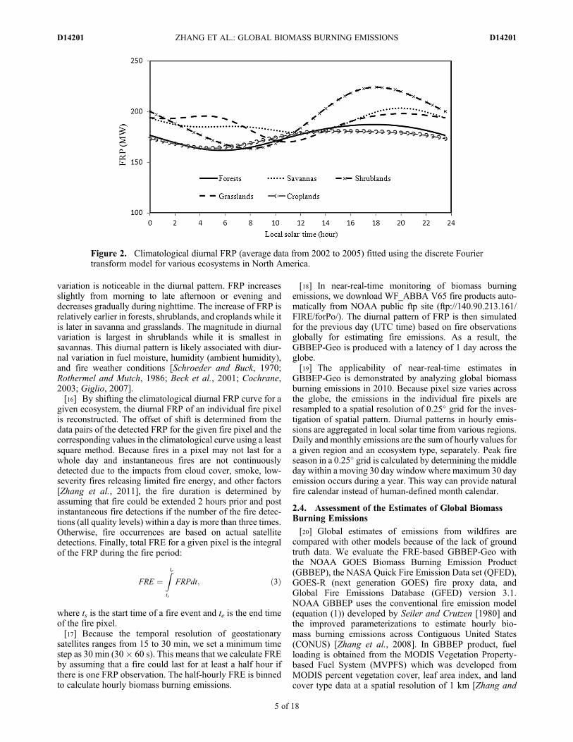
variation is noticeable in the diurnal pattern. FRP increasesslightly from morning to late afternoon or evening anddecreases gradually during nighttime. The increase of FRP isrelatively earlier in forests, shrublands, and croplands while itis later in savanna and grasslands. The magnitude in diurnalvariation is largest in shrublands while it is smallest insavannas. This diurnal pattern is likely associated with diur-nal variation in fuel moisture, humidity (ambient humidity),and fire weather conditions [Schroeder and Buck, 1970;Rothermel and Mutch, 1986; Beck et al., 2001; Cochrane,2003; Giglio, 2007].[16] By shifting the climatological diurnal FRP curve for a

given ecosystem, the diurnal FRP of an individual fire pixelis reconstructed. The offset of shift is determined from thedata pairs of the detected FRP for the given fire pixel and thecorresponding values in the climatological curve using a leastsquare method. Because fires in a pixel may not last for awhole day and instantaneous fires are not continuouslydetected due to the impacts from cloud cover, smoke, low-severity fires releasing limited fire energy, and other factors[Zhang et al., 2011], the fire duration is determined byassuming that fire could be extended 2 hours prior and postinstantaneous fire detections if the number of the fire detec-tions (all quality levels) within a day is more than three times.Otherwise, fire occurrences are based on actual satellitedetections. Finally, total FRE for a given pixel is the integralof the FRP during the fire period:

FRE ¼Zte

ts

FRPdt; ð3Þ

where ts is the start time of a fire event and te is the end timeof the fire pixel.[17] Because the temporal resolution of geostationary

satellites ranges from 15 to 30 min, we set a minimum timestep as 30 min (30� 60 s). This means that we calculate FREby assuming that a fire could last for at least a half hour ifthere is one FRP observation. The half-hourly FRE is binnedto calculate hourly biomass burning emissions.

[18] In near-real-time monitoring of biomass burningemissions, we download WF_ABBA V65 fire products auto-matically from NOAA public ftp site (ftp://140.90.213.161/FIRE/forPo/). The diurnal pattern of FRP is then simulatedfor the previous day (UTC time) based on fire observationsglobally for estimating fire emissions. As a result, theGBBEP-Geo is produced with a latency of 1 day across theglobe.[19] The applicability of near-real-time estimates in

GBBEP-Geo is demonstrated by analyzing global biomassburning emissions in 2010. Because pixel size varies acrossthe globe, the emissions in the individual fire pixels areresampled to a spatial resolution of 0.25� grid for the inves-tigation of spatial pattern. Diurnal patterns in hourly emis-sions are aggregated in local solar time from various regions.Daily and monthly emissions are the sum of hourly values fora given region and an ecosystem type, separately. Peak fireseason in a 0.25� grid is calculated by determining the middleday within a moving 30 day window where maximum 30 dayemission occurs during a year. This way can provide naturalfire calendar instead of human-defined month calendar.

2.4. Assessment of the Estimates of Global BiomassBurning Emissions

[20] Global estimates of emissions from wildfires arecompared with other models because of the lack of groundtruth data. We evaluate the FRE-based GBBEP-Geo withthe NOAA GOES Biomass Burning Emission Product(GBBEP), the NASA Quick Fire Emission Data set (QFED),GOES-R (next generation GOES) fire proxy data, andGlobal Fire Emissions Database (GFED) version 3.1.NOAA GBBEP uses the conventional fire emission model(equation (1)) developed by Seiler and Crutzen [1980] andthe improved parameterizations to estimate hourly bio-mass burning emissions across Contiguous United States(CONUS) [Zhang et al., 2008]. In GBBEP product, fuelloading is obtained from the MODIS Vegetation Property-based Fuel System (MVPFS) which was developed fromMODIS percent vegetation cover, leaf area index, and landcover type data at a spatial resolution of 1 km [Zhang and

Figure 2. Climatological diurnal FRP (average data from 2002 to 2005) fitted using the discrete Fouriertransform model for various ecosystems in North America.

ZHANG ET AL.: GLOBAL BIOMASS BURNING EMISSIONS D14201D14201

5 of 18

Kondragunta, 2006]. Fuel combustion efficiency and emis-sion factor vary with fuel moisture condition [Andersonet al., 2004], where the weekly fuel moisture category wasretrieved from AVHRR data [Zhang et al., 2008]. Burnedarea was simulated using half-hourly fire sizes obtained fromthe GOES-East WF_ABBA fire product [Zhang et al., 2008].We obtain GBBEP PM2.5 in 2010 from NOAA public ftpsite (ftp://satepsanone.nesdis.noaa.gov/EPA/GBBEP/) to eval-uate our FPR-based GBBEP-Geo results. Note that GBBEPonly uses GOES-East fire detections in emission estimates overCONUS while GBBEP-Geo combines GOES-East andGOES-West fire data. To make an appropriate comparison,we remove fire detections from GOES-W in GBBEP-Geoand only select the emission estimates from GOES-East.[21] We also compare our GBBEP-Geo with Quick Fire

Emission Data set Version 1 (QFED v1, http://geos5.org/wiki/index.php?title=Quick_Fire_Emission_Dataset_%28QFED%29). QFEDv1, the near-real-time biomass burning emissionsystem from the NASA Global Modeling and AssimilationOffice, produces daily total of black and organic carbon at aspatial resolution of 0.25 � 0.3125 degrees, which is derivedusing MODIS fire count and FRP products from both Aquaand Terra satellites. Similar to the approach developed byKaiser et al. [2009], cloud effects on FRP observations arereduced using the proportion of cloud cover. Terra MODISFRP andAquaMODIS FRP are then calibrated against GlobalFire Emissions Data version 2 (GFED2) [van der Werf et al.,2006], separately. This method accounts for the differencesin the fire strengths at the local time of the satellite overpassand ensures redundancy in case one of the satellites fails. Forthe comparison with QFEDv1, the total value of both blackand organic carbon is converted from dry mass in GBBEP-Geo using a coefficient of 0.009 [Chin et al., 2007].[22] The third data set used to assess the WF_ABBA FRP-

based biomass burning emissions is the GOES-R fire proxysimulated at CIRA (Cooperative Institute for Research in theAtmosphere), Colorado State University. This proxy simu-lates 4 GOES-R ABI (Advanced Baseline Imager) bands(2.25 mm, 3.9 mm, 10.35 mm, and 11.2 mm) that include firehot spots using a high-resolution Regional AtmosphericModeling System (RAMS) model [Grasso et al., 2008;Hillger et al., 2009]. The artificial fires were laid out in aregular grid size of 400 m and a temporal resolution of 5 min.Fire temperature that was artificially set spatially varied from400�K to 1200�K in 100�K intervals. Fires were set to varytemporally and weather conditions also changes. These firehot spots, which lasted 6 h, were simulated for 4 different fireevents which were detected by MODIS data on 23 October2007, California, 26 October 2007, California, 5 November2008, Arkansas, 24 April 2004, Central America. Fire tem-perature at the 400 m grids was used to calculate FRP. Thesesimulated FRP values calculated from fire temperature andfire grid size were also taken as the ground “truth” for eval-uation our global biomass emission algorithm.[23] The GOES-R ABI imagery at an approximately 2 � 2

km resolution was simulated using the anticipated pointspread function from the 400 m fires [Grasso et al., 2008;Hillger et al., 2009; Schmidt et al., 2010]. Based on thesesimulated instantaneous radiance, the WF_ABBA was usedto process the detection of fire characteristics. In theWF_ABBA output, fires may not always be detected and thefire characteristics may not be provided because of weak fire

emission, saturation, and cloud impacts. Fire detection rate islarger than 84% for fire pixel with FRP > 75 MW while verysmall fires are not detectable. The WF_ABBA FRP is thenused to estimate diurnal FRP variation and PM2.5 emissionsusing the GBBEP-Geo algorithm. The results are comparedwith simulated ground “truth” after the data pairs are aggre-gated to a temporal resolution of 1 hour. Because the factorsof converting FRE to biomass burning emissions in currentalgorithm are constant for a give fire event, the FRE differ-ence between proxy data and the estimates from GBBEP-Geo algorithm represents the quality of biomass burningemission estimates.[24] The fourth data set is GFED3.1. GFED3.1 provides

monthly biomass burning emissions from 1997 to 2010 at aspatial resolution of 0.5� using burned area and fuel loading[van der Werf et al., 2010]. Basically, biomass burningemissions were produced from a biogeochemical modelwhich employed monthly MODIS burned area and activefires, land cover characteristics, and plant productivity [vander Werf et al., 2010]. We obtain GFED3.1 data in 2010from a website (http://www.falw.vu/�gwerf/GFED/GFED3/emissions/). Monthly DM data are calculated from threeregions for comparing with GBBEP-Geo estimates, whichare South America, North America, and Africa.

3. Results

3.1. Spatial Pattern in Annual Global Biomass BurningEmissions

[25] Global wildfires release trace gases and aerosol with agreat spatial variability at both the fire pixel and the geo-graphical grid of 0.25� scales. Figure 3 shows the spatialpattern in annual biomass burning emissions for dry masscombustion, PM2.5 emissions, and CO emissions. The bio-mass burning emissions are large in South America andAfrica while the values are relatively small in Europe andAsia. In most parts of southern Brazil and Bolivia in SouthAmerica, dry mass combusted per grid cell is more than1.0 � 108 kg and emissions released per grid cell are morethan 1.0 � 106 kg of PM2.5 and 1.0 � 107 kg of CO. Simi-larly, large emissions in Africa occurred in Angola, Zambia,Botswana, Zimbabwe, Zaire, Rwanda, Burundi, and southernSudan. The largest biomass burning appeared in the bound-ary between northern Rwanda and eastern Zaire, where firesconsumed 4.3 � 109 kg of DM, and emitted 4.8 � 107 kg ofPM2.5 and 4.2 � 108 kg of CO in a 0.25� grid. However,emissions are not estimated for most of the regions in India,the Middle East, and boreal Asia (including Siberia) becauseof the lack of coverage from the multiple geostationarysatellites.[26] Biomass burning emissions vary greatly by continent

and ecosystem. Forest fires dominated in North America(region A), South America (region B), and Eastern Asia(region E), which burned forest dry mass of 7.17 � 1010 kg,1.50 � 1011 kg, and 6.17 � 1010 kg in 2010, separately(Figure 3 and Table 2). It accounts for 43.6%, 40.7% and39.5% of total dry mass burned in these correspondingregions. In contrast, savanna fires burned 4.52� 1011 kg and1.45 � 1010 kg of dry mass in Africa and Australia, sepa-rately, which accounts for 76.5% and 75.8% of total dry massburned across these regions. In Europe and Western Asia(region D), the amount of dry mass burned is similar for

ZHANG ET AL.: GLOBAL BIOMASS BURNING EMISSIONS D14201D14201

6 of 18

Figure 3

ZHANG ET AL.: GLOBAL BIOMASS BURNING EMISSIONS D14201D14201

7 of 18

forests, grasslands, and croplands. Globally, dry mass wasmostly consumed by savanna fires (47.8%), followed byforest fires (23.5%), shrubland fires (10.1%), cropland fires(9.0%), and grassland fires (9.7%). This pattern is mainly dueto the large dry mass combustion in Africa (44.6%) andSouth America (27.8%).[27] The spatial pattern and the relative proportion of

emissions in trace gases and aerosols are similar to that of drymass consumed (Tables 3 and 4). PM2.5 emissions are 6.1�109 kg in Africa, 3.4 � 109 kg in South America, 1.4 � 109

kg in Eastern Asia, and 1.4 � 109 kg North America. Simi-larly, CO emitted is 55.6 � 109 kg and 31.2 � 109 kg inAfrica and South America, separately. Patterns of fire emis-sions by ecosystem type match the patterns of dry biomassconsumed.

3.2. Seasonal Pattern in Global BiomassBurning Emissions

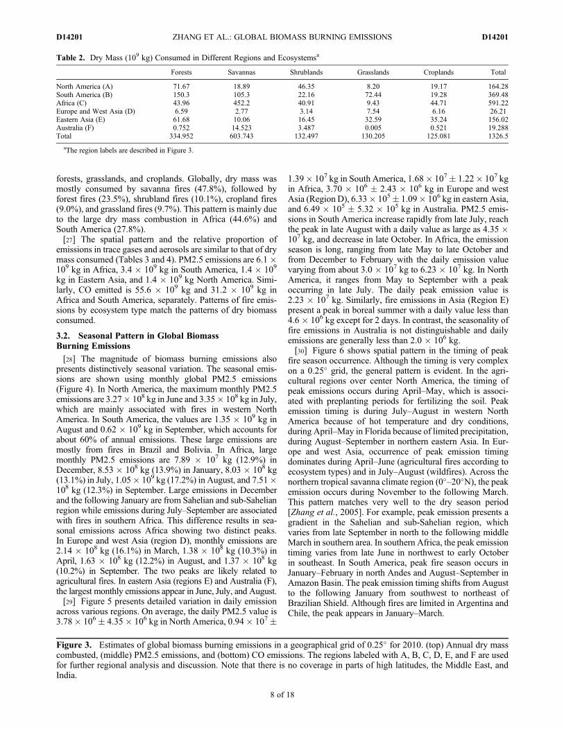
[28] The magnitude of biomass burning emissions alsopresents distinctively seasonal variation. The seasonal emis-sions are shown using monthly global PM2.5 emissions(Figure 4). In North America, the maximum monthly PM2.5emissions are 3.27� 108 kg in June and 3.35� 108 kg in July,which are mainly associated with fires in western NorthAmerica. In South America, the values are 1.35 � 109 kg inAugust and 0.62 � 109 kg in September, which accounts forabout 60% of annual emissions. These large emissions aremostly from fires in Brazil and Bolivia. In Africa, largemonthly PM2.5 emissions are 7.89 � 107 kg (12.9%) inDecember, 8.53 � 108 kg (13.9%) in January, 8.03 � 108 kg(13.1%) in July, 1.05� 109 kg (17.2%) in August, and 7.51�108 kg (12.3%) in September. Large emissions in Decemberand the following January are from Sahelian and sub-Sahelianregion while emissions during July–September are associatedwith fires in southern Africa. This difference results in sea-sonal emissions across Africa showing two distinct peaks.In Europe and west Asia (region D), monthly emissions are2.14 � 108 kg (16.1%) in March, 1.38 � 108 kg (10.3%) inApril, 1.63 � 108 kg (12.2%) in August, and 1.37 � 108 kg(10.2%) in September. The two peaks are likely related toagricultural fires. In eastern Asia (regions E) and Australia (F),the largest monthly emissions appear in June, July, and August.[29] Figure 5 presents detailed variation in daily emission

across various regions. On average, the daily PM2.5 value is3.78� 106� 4.35� 106 kg in North America, 0.94� 107�

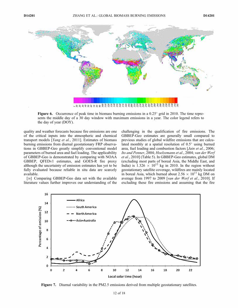
1.39� 107 kg in South America, 1.68� 107� 1.22� 107 kgin Africa, 3.70 � 106 � 2.43 � 106 kg in Europe and westAsia (Region D), 6.33� 105� 1.09� 106 kg in eastern Asia,and 6.49 � 105 � 5.32 � 105 kg in Australia. PM2.5 emis-sions in South America increase rapidly from late July, reachthe peak in late August with a daily value as large as 4.35 �107 kg, and decrease in late October. In Africa, the emissionseason is long, ranging from late May to late October andfrom December to February with the daily emission valuevarying from about 3.0 � 107 kg to 6.23 � 107 kg. In NorthAmerica, it ranges from May to September with a peakoccurring in late July. The daily peak emission value is2.23 � 107 kg. Similarly, fire emissions in Asia (Region E)present a peak in boreal summer with a daily value less than4.6� 106 kg except for 2 days. In contrast, the seasonality offire emissions in Australia is not distinguishable and dailyemissions are generally less than 2.0 � 106 kg.[30] Figure 6 shows spatial pattern in the timing of peak

fire season occurrence. Although the timing is very complexon a 0.25� grid, the general pattern is evident. In the agri-cultural regions over center North America, the timing ofpeak emissions occurs during April–May, which is associ-ated with preplanting periods for fertilizing the soil. Peakemission timing is during July–August in western NorthAmerica because of hot temperature and dry conditions,during April–May in Florida because of limited precipitation,during August–September in northern eastern Asia. In Eur-ope and west Asia, occurrence of peak emission timingdominates during April–June (agricultural fires according toecosystem types) and in July–August (wildfires). Across thenorthern tropical savanna climate region (0�–20�N), the peakemission occurs during November to the following March.This pattern matches very well to the dry season period[Zhang et al., 2005]. For example, peak emission presents agradient in the Sahelian and sub-Sahelian region, whichvaries from late September in north to the following middleMarch in southern area. In southern Africa, the peak emissiontiming varies from late June in northwest to early Octoberin southeast. In South America, peak fire season occurs inJanuary–February in north Andes and August–September inAmazon Basin. The peak emission timing shifts from Augustto the following January from southwest to northeast ofBrazilian Shield. Although fires are limited in Argentina andChile, the peak appears in January–March.

Figure 3. Estimates of global biomass burning emissions in a geographical grid of 0.25� for 2010. (top) Annual dry masscombusted, (middle) PM2.5 emissions, and (bottom) CO emissions. The regions labeled with A, B, C, D, E, and F are usedfor further regional analysis and discussion. Note that there is no coverage in parts of high latitudes, the Middle East, andIndia.

Table 2. Dry Mass (109 kg) Consumed in Different Regions and Ecosystemsa

Forests Savannas Shrublands Grasslands Croplands Total

North America (A) 71.67 18.89 46.35 8.20 19.17 164.28South America (B) 150.3 105.3 22.16 72.44 19.28 369.48Africa (C) 43.96 452.2 40.91 9.43 44.71 591.22Europe and West Asia (D) 6.59 2.77 3.14 7.54 6.16 26.21Eastern Asia (E) 61.68 10.06 16.45 32.59 35.24 156.02Australia (F) 0.752 14.523 3.487 0.005 0.521 19.288Total 334.952 603.743 132.497 130.205 125.081 1326.5

aThe region labels are described in Figure 3.

ZHANG ET AL.: GLOBAL BIOMASS BURNING EMISSIONS D14201D14201

8 of 18

3.3. Diurnal Variation in Biomass Burning Emissions

[31] Distinct diurnal patterns in hourly biomass burningemissions vary by region (Figure 7). PM2.5 emissions aremainly released from fires during 8:00–18:00 local solar time(LST) accounting for 80% of the daily emissions. In Africa,the diurnal pattern exhibits a normal distribution. The peakhour occurs around 13:00 with a maximum value of 15% ofthe daily total emissions. A similar diurnal pattern appears inNorth America with a peak hourly value of 11%. In contrast,the hourly emissions show a hat shape with a peak hourlyvalue of about 11% in South America and Asia and Australia,separately. The largest hourly emission occurs earlier in theday in Asia and Australia while it does later in SouthAmerica. The flat peak is associated with the peak shifts withland cover types [Giglio, 2007; Zhang and Kondragunta,2008]. In South America, the peak shifts about 1.5 hoursamong different land cover types. Moreover, the proportionof emissions in grasslands from 11:00 to 15:00 is very simi-lar, which results in a flat peak. It is likely that herbaceousvegetation provides finer and lighter fuels that dry outquickly, which could result in fire ignitions at any time of theday [Giglio, 2007]. The shift in the diurnal cycle is also likelyinfluenced by fire spread rates affected by synoptic-scalemeteorological events and weather conditions [French et al.,2011; Beck and Trevitt, 1989].[32] Overall, the result of diurnal pattern is comparable

with previous reports [Roberts et al., 2005, 2009; Giglio,2007; Justice et al., 2002; Zhang and Kondragunta, 2008;Mu et al., 2011]. Note that the diurnal pattern of total PM2.5emissions is generally controlled by the number of actual fireoccurrences, which is different from the climatological diurnalpattern of individual FRP values. The latter is referred to as themean FRP value in a given half hour if a fire is to occur.

3.4. Comparisons of GBBEP-Geo With OtherEstimates

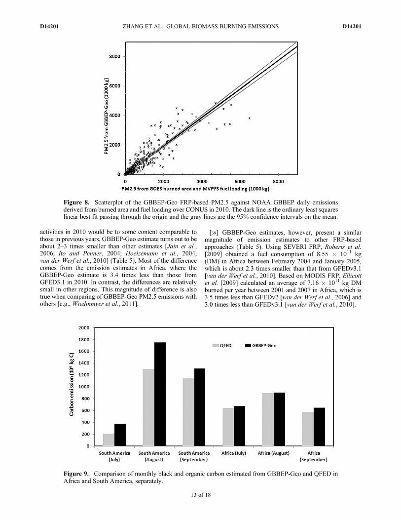
[33] Figure 8 presents the PM2.5 comparison betweenGBBEP-Geo estimates from FRP and GBBEP product cal-culated from burned area and fuel loading. The daily

emission values over CONUS are basically distributed alonga 1:1 line although there are a few outliers. The correlationbetween these two estimates is statistically significant (P <0.0001). The root-mean-square error (RMSE) in daily emis-sions is 4.99 � 105 kg for all of the samples. The linearregression (at 95% confidence) slope is 0.968 � 0.019 (P <0.00001), which indicates that there is no obvious biases. Thedetermination of correlation (R2) reveals that the GBBEP-Geo explains 88% of the variation in GBBEP. The differencein annual emissions shows that GBBEP-Geo is 5.7% largerthan GBBEP. This result indicates that the FRP-basedemission amount is overall equivalent to the estimates fromthe burned area and fuel loading approach. Because the firesources in these two estimates are all from GOES-East, theyhave the same omission and commission errors in firedetections. In other words, this comparison is not necessaryto validate the absolute magnitude of biomass burningemissions from GBBEP-Geo. Instead, it demonstrates thatthe FRP (or FRE) is an effective proxy to replace burned areaand fuel loading for the estimates of biomass burning emis-sions from wildfires.[34] Emission estimates from geostationary satellites are

also evaluated by comparing with the total emissions of bothblack and organic carbon from QFEDv1 in Africa and SouthAmerica (Figure 9). In Africa (around 25�S–5�N), themonthly emission value is similar in both data sets althoughGBBEP-Geo emissions are about 5%, 1%, and 13% largerthan QFEDv1 emissions in July, August, and September,separately. In contrast, the monthly QFEDv1 emission inSouth America (around 35�S–10�N) is about 54%, 75%, and87% of GBBEP-Geo value in July, August, and September,separately. Overall, their values during these 3 months arecomparable with a ratio (GBBEP-Geo/QFED) of 1.3 and 1.1in South America and Africa. This means that these two esti-mates are strongly comparable, particularly in Africa.[35] Figure 10 shows the FRE comparison between ground

“truth” of the simulated GOES-R fire proxy data and esti-mates derived from GBBEP-Geo algorithm. The resultsindicate that FRE values are well estimated for small/weak

Table 3. PM2.5 Emissions (109 kg) in Different Regions and Ecosystemsa

Forests Savannas Shrublands Grasslands Croplands Total

North America (A) 0.714 0.188 0.281 0.070 0.099 1.352South America (B) 1.50 1.05 0.134 0.621 0.099 3.404Africa (C) 0.487 5.006 0.274 0.090 0.255 6.112Europe and West Asia (D) 0.073 0.031 0.021 0.072 0.035 0.232East Asia (E) 0.683 0.111 0.110 0.310 0.201 1.415Australia (F) 0.008 0.161 0.023 0.00004 0.003 0.196Total 3.465 6.547 0.843 1.163 0.692 12.711

aThe region labels are described in Figure 3.

Table 4. CO Emissions (109 kg) in Different Regions and Ecosystemsa

Forests Savannas Shrublands Grasslands Croplands Total

North America (A) 6.266 1.652 3.59 0.665 1.211 13.384South America (B) 13.15 9.217 1.717 5.88 1.219 31.185Africa (C) 4.265 43.864 3.518 0.849 3.129 55.624Europe and West Asia (D) 0.639 0.269 0.271 0.679 0.432 2.289East Asia (E) 5.983 0.976 1.414 2.933 2.467 13.773Australia (F) 0.073 1.409 0.300 0.0004 0.036 1.819Total 30.378 57.387 10.81 11.006 8.494 118.074

aThe region labels are described in Figure 3.

ZHANG ET AL.: GLOBAL BIOMASS BURNING EMISSIONS D14201D14201

9 of 18

Figure 4. Monthly PM2.5 burning emissions aggregated in a 0.25� grid across the globe in 2010. Notethat there is no coverage in parts of high latitudes, the Middle East, and India.

ZHANG ET AL.: GLOBAL BIOMASS BURNING EMISSIONS D14201D14201

10 of 18

fires while the values are underestimated for large/strongfires. Overall the hourly mean FRE estimated accounts for90% of the variation in the “truth.”As a whole of the four fireevents, the total FRE estimated from the GBBEP-Geo is12.4% smaller than “truth.” This FRE difference representsthe quality of biomass burning emissions because the factorused to convert FRE to emissions in current algorithm isconstant.[36] Figure 11 indicates that monthly DM in GBBEP-Geo

is significantly correlated with GFED3.1 estimate in Africa(R2 = 0.89), in South America (R2 = 0.88), and in NorthAmerica (R2 = 0.85). However, the magnitude is discrepant.In African, monthly GBBEP-Geo DM is consistently smallerthan GFEDv3.1 estimate with a factor larger than 2, whichleads to a factor of 3.4 in annual DM. In South America,GBBEP-Geo DM is smaller than GFEDv3.1 DM fromMay toOctober while it is larger during other months. Because theemission estimates differ greatly in the fire peak season(August and September) in 2010, which accounts for 85% of

annual emissions in GFEDv3.1 and 57% in GBBEP-Geo, theannual DM in GBBEP-Geo is smaller than GFEDv3.1 esti-mate with a factor of 3.8. In North America, GBBEP-Geo DMis slightly smaller than GFEDv3.1 estimate with a factor of1.36, which is mainly due to the large difference in June andJuly. In contrast, DM is larger in GBBEP-Geo than inGFEDv3.1 with a factor of 2.1 in the region of temperateNorth America and Central America. Similarly, GFED gen-erally produces relatively lower fire emissions in this regioncomparing with other studies [Al-Saadi et al., 2008; Kaiseret al., 2012].

4. Discussion

[37] The high frequency of fire observations from multiplegeostationary satellites enables us to estimate global biomassburning emissions in near real time. The operational productof GBBEP-Geo could meet the needs to provide hourlyemissions in near real time from individual fire pixels for air

Figure 5. Daily PM2.5 emissions estimated from multiple geostationary satellites over the six regions in2010.

ZHANG ET AL.: GLOBAL BIOMASS BURNING EMISSIONS D14201D14201

11 of 18

quality and weather forecasts because fire emissions are oneof the critical inputs into the atmospheric and chemicaltransport models [Yang et al., 2011]. Estimates of biomassburning emissions from diurnal geostationary FRP observa-tions in GBBEP-Geo greatly simplify conventional modelparameters of burned area and fuel loading. The applicabilityof GBBEP-Geo is demonstrated by comparing with NOAAGBBEP, QFEDv1 estimates, and GOES-R fire proxyalthough the uncertainty of emission estimates has yet to befully evaluated because reliable in situ data are scarcelyavailable.[38] Comparing GBBEP-Geo data set with the available

literature values further improves our understanding of the

challenging in the qualification of fire emissions. TheGBBEP-Geo estimates are generally small compared toprevious studies of global wildfire emissions that are calcu-lated monthly at a spatial resolution of 0.5� using burnedarea, fuel loading and combustion factors [Jain et al., 2006;Ito and Penner, 2004; Hoelzemann et al., 2004; van der Werfet al., 2010] (Table 5). In GBBEP-Geo estimates, global DM(excluding most parts of boreal Asia, the Middle East, andIndia) is 1.326 � 1012 kg in 2010. In the region withoutgeostationary satellite coverage, wildfires are mainly locatedin boreal Asia, which burned about 2.56 � 1011 kg DM onaverage from 1997 to 2009 [van der Werf et al., 2010]. Ifexcluding these fire emissions and assuming that the fire

Figure 6. Occurrence of peak time in biomass burning emissions in a 0.25� grid in 2010. The time repre-sents the middle day of a 30 day window with maximum emissions in a year. The color legend refers tothe day of year (DOY).

Figure 7. Diurnal variability in the PM2.5 emissions derived from multiple geostationary satellites.

ZHANG ET AL.: GLOBAL BIOMASS BURNING EMISSIONS D14201D14201

12 of 18

activities in 2010 would be to some content comparable tothose in previous years, GBBEP-Geo estimate turns out to beabout 2–3 times smaller than other estimates [Jain et al.,2006; Ito and Penner, 2004; Hoelzemann et al., 2004,van der Werf et al., 2010] (Table 5). Most of the differencecomes from the emission estimates in Africa, where theGBBEP-Geo estimate is 3.4 times less than those fromGFED3.1 in 2010. In contrast, the differences are relativelysmall in other regions. This magnitude of difference is alsotrue when comparing of GBBEP-Geo PM2.5 emissions withothers [e.g., Wiedinmyer et al., 2011].

[39] GBBEP-Geo estimates, however, present a similarmagnitude of emission estimates to other FRP-basedapproaches (Table 5). Using SEVERI FRP, Roberts et al.[2009] obtained a fuel consumption of 8.55 � 1011 kg(DM) in Africa between February 2004 and January 2005,which is about 2.3 times smaller than that from GFEDv3.1[van der Werf et al., 2010]. Based on MODIS FRP, Ellicottet al. [2009] calculated an average of 7.16 � 1011 kg DMburned per year between 2001 and 2007 in Africa, which is3.5 times less than GFEDv2 [van der Werf et al., 2006] and3.0 times less than GFEDv3.1 [van der Werf et al., 2010].

Figure 8. Scatterplot of the GBBEP-Geo FRP-based PM2.5 against NOAA GBBEP daily emissionsderived from burned area and fuel loading over CONUS in 2010. The dark line is the ordinary least squareslinear best fit passing through the origin and the gray lines are the 95% confidence intervals on the mean.

Figure 9. Comparison of monthly black and organic carbon estimated from GBBEP-Geo and QFED inAfrica and South America, separately.

ZHANG ET AL.: GLOBAL BIOMASS BURNING EMISSIONS D14201D14201

13 of 18

[40] The modeled results using the Seiler and Crutzen[1980] equation are largely dependent on the input qualityof burned area, fuel loading, and combustion factors [e.g.,van der Werf et al., 2010; Hoelzemann et al., 2004].Although global burned area has been greatly improved withthe development of high-resolution satellite data from 500 mto 1 km [Roy et al., 2008; Plummer et al., 2006; Tansey et al.,2008; Giglio et al., 2009], the discrepancy among varioussatellite-based global products is still very large [Giglio et al.,2010; Roy and Boschetti, 2009; van der Werf et al., 2010;Conard et al., 2002; Boschetti et al., 2004]. The differencecould be as large as from 2 to 10 times in some regions

because of the impacts from unburned patches in a fire pixeland persistent cloud and smoke [Conard et al., 2002;Boschetti et al., 2004]. Global fuel loading is generallyderived from land cover types and biomass density data[Ito and Penner, 2004; Jain et al., 2006; Wiedinmyer et al.,2011], global vegetation model [Hoelzemann et al., 2004],and global biogeochemical models [van der Werf et al.,2006]. The related uncertainty could result in a discrepancyof as large as 4 times [Campbell et al., 2007]. Combustionfactor depends on fuel type and burn severity. The combus-tion factor for forest wood is about 0.3–0.5 in most models[e.g., Ito and Penner, 2004; Soja et al., 2004; Wiedinmyer

Figure 10. Comparison of hourly FRE calculated fromWF_ABBA detected from the fire proxy radiancewith fire proxy FRE in the four proxy fire events.

Figure 11. Comparison of DM between GFED3.1 and GBBEP-Geo estimates in 2010.

ZHANG ET AL.: GLOBAL BIOMASS BURNING EMISSIONS D14201D14201

14 of 18

et al., 2006; Jain et al., 2006], which is much larger thansome detailed field calculations [Campbell et al., 2007;Meigs et al., 2009]. It is likely that previous emission esti-mates commonly use combustion factor obtained fromhigh-severity fires for all fire regimes, although low- andmoderate-severity fires account for majority proportion inlarge wildfires [Schwind, 2008; Miller et al., 2009; Zhanget al., 2011].[41] The FRP algorithm avoids the uncertainty in burned

area, fuel loading, and combustion factor, but the results areinfluenced by FRP detection and biomass combustion rate(b). Although it is not easy to directly validate satellite FRPmeasurements, the FRP values detected from GOES Imagerand Meteosat SEVERI have been shown to agree withMODIS FRP retrievals [Roberts et al., 2005; Xu et al., 2010].However, at the regional scale SEVIRI typically under-estimates FRP by up to 40% with respect to MODIS dueprimarily to its inability to confidently detect fire pixelswith FRP ≤ 100 MW [Roberts et al., 2005]. GOES FRP isundetected for many fire pixels having FRP < 30 MW andso GOES measurements could be on average 17% lower[Xu et al., 2010].[42] Moreover, the uncertainty of FRP in the GBBEP-Geo

also comes from the satellite viewing angles. Fire character-ization detections are based on the proportion of the pixel onfire. For pixels near the geostationary satellite limb, a largerfire area is necessary to create the same fire proportion as apixel near the subsatellite point. As viewing angle increases,pixel size increases and the probability of detecting smallerand less intense fires decreases [Giglio et al., 1999; Freebornet al., 2011]. As a result, the minimum detectable FRPincreases toward the large viewing angles. Similar to MODISFRE [Freeborn et al., 2011], the viewing angle effect ofgeostationary satellites results in the underestimates of actualfire FRE. This effect is under investigation and will beincluded in the next version of GBBEP-Geo product.[43] Although our simulated diurnal FRP values for a fire

pixel are expected to compensate for fire detections withoutFRP calculations and some undetected fires, some uncertain-ties also exist. The shape of FRP diurnal pattern for individualfires varies slightly with different regions. Currently the cli-matological FRP shape generated using GOES fire detectionsin North America is applied to globe. After comparing theclimatological pattern in North America with that in Africaduring 2009 and 2010, we found the shape variation couldcause an uncertainty of about 7%.

[44] The biomass combustion rate in FRE also causescertain uncertainty although it is shown not to vary with fueltypes. Field controlled experiments (29 samples) demon-strate that the FRE combustion factor is 0.368� 0.015 kg/MJregardless the land ecosystem types [Wooster et al., 2005].However, laboratory-controlled experiments in a combustionchamber demonstrate that the rate of dry fuels combusted perFRP unit ranges from 0.24 to 0.78 kg/MJ with an overallregression rate of 0.453 � 0.068 kg/MJ [Freeborn et al.,2008]. In GBBEP-Geo, we adopt the coefficient of 0.368kg/MJ, which is 23% lower than the 0.453 kg/MJ.[45] The above biomass combustion rate in FRE from

laboratory-controlled experiments differs greatly from thatobtained from other sources. In the GFASv0, the combustionrate is 1.37 kg/MJ that was obtained following a comparisonof global MODIS FRE to emissions in GFED2 inventory[Kaiser et al., 2009]. The aerosol optical thickness (AOT)simulated from FRE-based emissions (GFASv1.0) is lowerthan MODIS AOT by a factor of 3.4 [Kaiser et al., 2012].Similarly, the AOT simulated using MODIS FRE-derivedfire emissions is less than MODIS AOT with factors of 1.8 insavannah and grasslands, 2.5 in tropical forest and 4.5 inextratropical forest [Colarco et al., 2011]. This large dis-crepancy between bottom-up and top-down AOT estimates isunclear, which is likely caused by various factors that includethe rapid changes of smoke particles with age [Reid et al.,1998], the uncertainty in climate and atmospheric transportmodels, and underestimate of the biomass combustion factorand FRE.[46] Moreover, the combustion rate in FRE is considerably

large when comparing MODIS FRE with MODIS smokeAOT. The comparison indicates a FRE-based emission factorfor total particulate mass (PM) is 0.02–0.06 kg/MJ for borealregions, 0.04–0.08 kg/MJ for both tropical forests and savannaregions, and 0.08–0.1 kg/MJ for Western Russian regions[Ichoku and Kaufman, 2005]. If the rate of total PM emissionsis converted to burned DM using PM2.5 emission factors inGFED3.1 [van derWerf et al., 2010] and the ratio between totalPM and PM2.5 [Sofiev et al., 2009], the biomass combustionrate in FRE roughly ranges from 2 to 12 kg/MJ. However, thesecoefficients may be overestimated by about 50% [Ichoku andKaufman, 2005]. Similarly, the emission coefficient for totalPM in Europe is 0.035 kg/MJ for forest, 0.018 kg/MJ forgrassland and agriculture, and 0.026 kg/MJ for mixed vegeta-tion [Sofiev et al., 2009]. These values are roughly associated toa biomass combustion rate of 1.6–2.2 kg/MJ. These results

Table 5. Comparisons of Annual Dry Mass Combustion (109 kg) From Various Studiesa

Methods Global Africa North America South AmericaSpatiotemporalResolution Year of Fires Reference

Equation (1) 3099–4159 1712–2654 164–405 145–181 month, 0.5� 2000 Jain et al. [2006]Equation (1) 2797–3814 1824–2705 61–64 176–188 month, 1 km 2000 Ito and Penner [2004]Equation (1) 2730–4056 NAb NA NA month, 0.5� 2000 Hoelzemann et al. [2004]Equation (1) 4539 2058 222 1407 month, 0.5� 2010 van der Werf et al. [2010]Equation (2) NA 855 NA NA day, 1� 2004 Roberts et al. [2009]Equation (2) NA 716 NA NA month, 0.5� 2001–2007 Ellicott et al. [2009]Equation (2) 1326c 591 164 369 hour, pixel size 2010 This study

aEquation (1) represents the model based on burned area and biomass density (fuel loading) and equation (2) indicates the FRP method. The range ofestimates in Jain et al. [2006] and Ito and Penner [2004] is the result of two different burned areas used.

bNA: Not available.cNo coverage for most regions in boreal Asia, the Middle East, and India.

ZHANG ET AL.: GLOBAL BIOMASS BURNING EMISSIONS D14201D14201

15 of 18

indicate that the rate of biomass combustion in FRE from sta-tistical comparisons between various data sets is much largerthan that from laboratory-controlled experiments. We believethat the factor of converting FRE to biomass burning emis-sions needs further investigation.[47] Emission factor is another source of the uncertainty in

the estimates of biomass burning emissions. In regional andglobal scales, emission factors are highly aggregated to a fewecosystem types. Consequently, the values vary with the fieldmeasurements available and the ecosystem types classified[Akagi et al., 2011; van der Werf et al., 2010; Wiedinmyeret al., 2006, 2011]. The uncertainty among these studies isconsistent with that from field measurements for manyimportant species, which is about 20–30% [Andreae andMerlet, 2001]. However, the emission factors of PM2.5 areabout four times larger in various studies [e.g., van der Werfet al., 2010; Wiedinmyer et al., 2011] than those conductedby Urbanski et al. [2011]. Our GBBEP-Geo algorithm cur-rently uses the factors from the literature [Wiedinmyer et al.,2006], which is intended to updated using newly availabledata [Akagi et al., 2011; Wiedinmyer et al., 2011].[48] Finally, the GBBEP-Geo does not produce biomass

burning emissions from fires that occur in most regions of theMiddle East, India and boreal Asia because of the lack ofcoverage from current geostationary satellites. For thisregion, boreal Asia is one of the most important fire regimes[Soja et al., 2004], which releases 6.4% of global wildfireemissions [van der Werf et al., 2010]. To overcome thislimitation for investigating global biomass burning emis-sions, INSAT-3D, a geostationary satellite developed by theIndian Space Research Organization and expected to belaunched in 2011, is expected to fill the gap.

5. Conclusions

[49] Fire radiative power estimated from multiple geosta-tionary satellites provides an indispensable tool to calculateglobal biomass burning emissions in near real time on anhourly time scale. This product will significantly contributeto air quality and weather forecasting. The estimate of bio-mass burning emissions from FRP avoids using the complexparameters of fuel loading and burned area. Thus, it is arobust approach for the global estimates of biomass burningemissions. High frequent fire observations from geostation-ary satellites allow us to reconstruct the diurnal pattern inFRP for individual fire pixels. This increases the number ofobservations that otherwise would not be reported due tocloud/smoke cover.[50] Note that high uncertainty exists in global biomass

emissions and accurate validation is currently not possiblebecause of the lack of reliable in situ measurement. Inter-composition among different products reveals that the FRP-based GBBEP-Geo estimates are generally smaller thanprevious global calculations from burned area and fuelloading with a factor of 2–3. However, GBBEP-Geo iscomparable with emission estimates from GOES-basedburned area and MODIS-based fuel loadings in the UnitedStates, from MODIS-based FRP, and from SEVERI-basedFRP in Africa. Thus, it is evident that GBBEP-Geo producesreliable estimates of biomass burning emissions from wild-fires. Finally, it should be noted that GBBEP-Geo currently

provides limited coverage in high latitudes and no coveragein most regions across India and parts of boreal Asia.

[51] Acknowledgments. The authors thank Arlindo da Silva in NASAfor providing QFED v1 data, Manajit Sengupta and Renate Brummer for fireproxy data, Gilberto Vicente for internal reviews, and four anonymousreviewers for constructive comments. The views, opinions, and findingscontained in these works are those of the author(s) and should not be inter-preted as an official NOAA or U.S. government position, policy, or decision.

ReferencesAkagi, S. K., R. J. Yokelson, C. Wiedinmyer, M. J. Alvarado, J. S. Reid,T. Karl, J. D. Crounse, and P. O. Wennberg (2011), Emission factorsfor open and domestic biomass burning for use in atmospheric models,Atmos. Chem. Phys., 11, 4039–4072, doi:10.5194/acp-11-4039-2011.

Al-Saadi, J., et al. (2008), Intercomparison of near-real-time biomass burn-ing emissions estimates constrained by satellite fire data, J. Appl. RemoteSens., 2, 021504, doi:10.1117/1.2948785.

Anderson, G. K., D. V. Sandberg, and R. A. Norheim (2004), Fire EmissionProduction Simulator (FEPS) user’s guide, version 1.0, For. Serv., U.S.Dep. of Agric., Portland, Oreg. [Available at http://www.fs.fed.us/pnw/fera/publications/fulltext/FEPS_User_Guide.pdf.]

Andreae, M. O., and P. Merlet (2001), Emission of trace gases and aerosolsfrom biomass burning, Global Biogeochem. Cycles, 15(4), 955–966,doi:10.1029/2000GB001382.

Beck, J. A., and A. C. F. Trevitt (1989), Forecasting diurnal variations inmeteorological parameters for predicting fire behaviour, Can. J. For.Res., 19, 791–797, doi:10.1139/x89-120.

Beck, J. A., M. E. Alexander, S. D. Harvey, and A. K. Beaver (2001), Fore-casting diurnal variation in fire intensity for use in wildland fire manage-ment applications, paper presented at Fourth Symposium on Fire andForest Meteorology, Am. Meteorol. Soc., Reno, Nev., 13–15 Nov.

Boschetti, L., H. D. Eva, P. A. Brivio, and J. M. Grégoire (2004), Lessonsto be learned from the comparison of three satellite-derived biomass burn-ing products, Geophys. Res. Lett., 31, L21501, doi:10.1029/2004GL021229.

Brown, J. F., T. R. Loveland, D. O. Ohlen, and Z. Zhu (1999), The globalland-cover characteristics data-base: The users’ perspective, J. Am. Soc.Photogramm. Remote Sens., 65(9), 1069–1074.

Campbell, J., D. Donato, D. Azuma, and B. Law (2007), Pyrogenic carbonemission from a large wildfire in Oregon, United States, J. Geophys. Res.,112, G04014, doi:10.1029/2007JG000451.

Chin, M., T. Diehl, P. Ginoux, and W. Malm (2007), Intercontinental trans-port of pollution and dust aerosols: Implications for regional air quality,Atmos. Chem. Phys., 7, 5501–5517, doi:10.5194/acp-7-5501-2007.

Cochrane, M. A. (2003), Fire science for rainforests, Nature, 421, 913–919,doi:10.1038/nature01437.

Colarco, P., et al. (2011), The NASA GEOS-5 aerosol forecasting sys-tem, paper presented at the MACC Conference on Monitoring andForecasting Atmospheric Composition, Eur. Cent. for Medium RangeWeather Forecasts, Utrecht, Netherlands, 23–27 May.

Conard, S. G., A. I. Sukhinin, B. J. Stocks, D. R. Cahoon, E. P. Davidenko,and G. A. Ivanova (2002), Determining effects of area burned and fireseverity on carbon cycling and emissions in Siberia, Clim. Change, 55,197–211.

Ellicott, E., E. Vermote, L. Giglio, and G. Roberts (2009), Estimating bio-mass consumed from fire using MODIS FRE, Geophys. Res. Lett., 36,L13401, doi:10.1029/2009GL038581.

Freeborn, P. H., M. J. Wooster, W. M. Hao, C. A. Ryan, B. L. Nordgren,S. P. Baker, and C. Ichoku (2008), Relationships between energyrelease, fuel mass loss, and trace gas and aerosol emissions during lab-oratory biomass fires, J. Geophys. Res., 113, D01301, doi:10.1029/2007JD008679.

Freeborn, P. H., M. J. Wooster, and G. Roberts (2011), Addressing the spatio-temporal sampling design of MODIS to provide estimates of the fire radia-tive energy emitted from Africa, Remote Sens. Environ., 115, 475–489,doi:10.1016/j.rse.2010.09.017.

French, N. H. F., et al. (2011), Model comparisons for estimating carbonemissions from North American wildland fire, J. Geophys. Res., 116,G00K05, doi:10.1029/2010JG001469.

Galanter, M., H. Levy II, and G. R. Carmichael (2000), Impacts of bio-mass burning on tropospheric CO, NOx, and O3, J. Geophys. Res.,105, 6633–6653.

Giglio, L. (2007), Characterization of the tropical diurnal fire cycle usingVIRS and MODIS observations, Remote Sens. Environ., 108, 407–421,doi:10.1016/j.rse.2006.11.018.

ZHANG ET AL.: GLOBAL BIOMASS BURNING EMISSIONS D14201D14201

16 of 18

Giglio, L., J. D. Kendall, and C. O. Justice (1999), Evaluation of global firedetection algorithms using simulated AVHRR infrared data, Int. J. RemoteSens., 20, 1947–1985, doi:10.1080/014311699212290.

Giglio, L., J. D. Kendall, and R. Mack (2003), A multi-year active fire data-set for the tropics derived from the TRMM VIRS, Int. J. Remote Sens.,24, 4505–4525.

Giglio, L., T. Loboda, D. P. Roy, B. Quayle, and C. O. Justice (2009), Anactive-fire based burned area mapping algorithm for the MODIS sensor,Remote Sens. Environ., 113, 408–420, doi:10.1016/j.rse.2008.10.006.

Giglio, L., J. T. Randerson, G. R. van der Werf, P. S. Kasibhatla, G. J.Collatz, D. C. Morton, and R. S. DeFries (2010), Assessing variabilityand long-term trends in burned area by merging multiple satellite fireproducts, Biogeosciences, 7, 1171–1186, doi:10.5194/bg-7-1171-2010.

Grasso, L., M. Sengupta, and D. T. Lindsey (2008), Synthetic GOES-Rimagery development and uses, paper presented at Fifth GOES Users’Conference, NOAA, New Orleans, La., 23–24 Jan.

Hao, W. M., and M.-H. Liu (1994), Spatial and temporal distribution oftropical biomass burning, Global Biogeochem. Cycles, 8, 495–503.

Hao, W. M., M.-H. Liu, and P. J. Crutzen (1990), Estimates of annual andregional releases of CO2 and other trace gases to the atmosphere from firesin the tropics, based on the FAO statistics for the period 1975–80, in Firein the Tropical Biota: Ecosystem Processes and Global Challenges, Ecol.Stud., vol. 84, edited by J. G. Goldammer, pp. 440–462, Springer, NewYork.

Hillger, D., M. DeMaria, R. Brummer, L. Grasso, M. Sengupta, andR. DeMaria (2009), Production of proxy datasets in support of GOES-Ralgorithm development, Proc. SPIE Int. Soc. Opt. Eng., 7458, 74580C,doi:10.1117/12.828489.

Hoelzemann, J. J., M. G. Schultz, G. P. Brasseur, C. Granier, and M. Simon(2004), Global Wildland Fire Emission Model (GWEM): Evaluating theuse of global area burnt satellite data, J. Geophys. Res., 109, D14S04,doi:10.1029/2003JD003666.

Ichoku, C., and Y. J. Kaufman (2005), A method to derive smoke emissionrates fromMODIS fire radiative energy measurements, IEEE Trans. Geosci.Remote Sens., 43(11), 2636–2649, doi:10.1109/TGRS.2005.857328.

Ichoku, C., L. Giglio, M. J. Wooster, and L. A. Remer (2008), Global char-acterization of biomass-burning patterns using satellite measurements offire radiative energy, Remote Sens. Environ., 112, 2950–2962,doi:10.1016/j.rse.2008.02.009.

Ito, A., and J. E. Penner (2004), Global estimates of biomass burning emis-sions based on satellite imagery for the year 2000, J. Geophys. Res., 109,D14S05, doi:10.1029/2003JD004423.

Jain, A. K., Z. Tao, X. Yang, and C. Gillespie (2006), Estimates of globalbiomass burning emissions for reactive greenhouse gases (CO, NMHCs,and NOx) and CO2, J. Geophys. Res., 111, D06304, doi:10.1029/2005JD006237.

Justice, C. O., J. R. G. Townshend, E. F. Vermote, E. Masuoka, R. E. Wolfe,N. Saleous, D. P. Roy, and J. T. Morisette (2002), An overview of MODISland data processing and product status, Remote Sens. Environ., 83, 3–15.

Kaiser, J. W., J. Flemming, M. G. Schultz, M. Suttie, and M. J. Wooster(2009), The MACC global fire assimilation system: First emission pro-ducts (GFASv0), ECMWF Tech. Memo. 596, 18 pp., Eur. Cent. forMedium Range Weather Forecasts, Reading, U. K.

Kaiser, J. W., et al. (2012), Biomass burning emissions estimated with aglobal fire assimilation system based on observed fire radiative power,Biogeosciences, 9, 527–554, doi:10.5194/bg-9-527-2012.

Kaufman, Y. J., C. O. Justice, L. P. Flynn, J. D. Kendall, E. M. Prins,L. Giglio, D. E. Ward, W. P. Menzel, and A. W. Setzer (1998),Potential global fire monitoring from EOS-MODIS, J. Geophys.Res., 103(D24), 32,215–32,238, doi:10.1029/98JD01644.

Langenfelds, R. L., R. J. Francey, B. C. Pak, L. P. Steele, J. Lloyd, C. M.Trudinger, and C. E. Allison (2002), Interannual growth rate variationsof atmospheric CO2 and its d13C, H2, CH4, and CO between 1992 and1999 linked to biomass burning, Global Biogeochem. Cycles, 16(3),1048, doi:10.1029/2001GB001466.

Lobert, J., and J. Warnatz (1993), Emissions from the combustion processin vegetation, in Fire in the Environment: The Ecological, Atmospheric,and Climatic Importance of Vegetation Fires, Environ. Sci. Res. Rep.,vol. 13, edited by P. J. Crutzen and J. G. Goldammer, pp. 15–39, JohnWiley, New York.

Lobert, J. M., W. C. Keene, J. A. Logan, and R. Yevich (1999), Globalchlorine emissions from biomass burning: Reactive Chlorine EmissionsInventory, J. Geophys. Res., 104, 8373–8389.

Meigs, G. W., D. C. Donato, J. L. Campbell, J. G. Martin, and B. E. Law(2009), Forest fire impacts on carbon uptake, storage, and emission:The role of burn severity in the eastern Cascades, Oregon, Ecosystems,12(8), 1246–1267, doi:10.1007/s10021-009-9285-x.

Miller, J. D., H. D. Safford, M. Crimmins, and A. E. Thode (2009), Quan-titative evidence for increasing forest fire severity in the Sierra Nevada

and southern Cascade Mountains, California and Nevada, USA, Ecosys-tems, 12, 16–32, doi:10.1007/s10021-008-9201-9.

Mu, M., et al. (2011), Daily and 3-hourly variability in global fire emissionsand consequences for atmospheric model predictions of carbon monox-ide, J. Geophys. Res., 116, D24303, doi:10.1029/2011JD016245.

Piccolini, I., and O. Arino (2000), Towards a global burned surface worldatlas, Earth Obs. Q., 65, 14–18.

Plummer, S., O. Arino, M. Simon, and W. Steffen (2006), Establishing aEarth observation product service for the terrestrial carbon community:The Globcarbon Initiative, Mitigation Adaptation Strategies GlobalChange, 11, 97–111.

Prins, E. M., and W. P. Menzel (1992), Geostationary satellite detection ofbiomass burning in South America, Int. J. Remote Sens., 13, 2783–2799.

Prins, E. M., J. M. Feltz, W. P. Menzel, and D. E. Ward (1998), An over-view of GOES-8 diurnal fire and smoke results for SCAR-B and 1995 fireseason in South America, J. Geophys. Res., 103(D24), 31,821–31,835,doi:10.1029/98JD01720.

Reid, J. S., P. V. Hobbs, R. J. Ferek, D. R. Blake, J. V. Martins, M. R. Dunlap,and C. Liousse (1998), Physical, chemical, and optical properties of regionalhazes dominated by smoke in Brazil, J. Geophys. Res., 103, 32,059–32,080,doi:10.1029/98JD00458.

Reid, J. S., E. M. Prins, D. L. Westphal, C. C. Schmidt, K. A. Richardson,S. A. Christopher, T. F. Eck, E. A. Reid, C. A. Curtis, and J. P. Hoffman(2004), Real-time monitoring of South American smoke particle emis-sions and transport using a coupled remote sensing/box-model approach,Geophys. Res. Lett., 31, L06107, doi:10.1029/2003GL018845.

Roberts, G., M. J. Wooster, G. L. W. Perry, N. Drake, L.-M. Rebelo, andF. Dipotso (2005), Retrieval of biomass combustion rates and totalsfrom fire radiative power observations: Application to southern Africausing geostationary SEVIRI imagery, J. Geophys. Res., 110, D21111,doi:10.1029/2005JD006018.

Roberts, G., M. J. Wooster, and E. Lagoudakis (2009), Annual and diurnalAfrican biomass burning temporal dynamics, Biogeosciences, 6, 849–866,doi:10.5194/bg-6-849-2009.

Rothermel, R. C., and R. W. Mutch (1986), Behavior of the life-threateningButte fire: August 27–29, 1985, Fire Manage. Notes, 47(2), 14–24.

Roy, D. P., and L. Boschetti (2009), Southern Africa validation of theMODIS, L3JRC, and GlobCarbon burned-area products, IEEE Trans.Geosci. Remote Sens., 47, 1032–1044, doi:10.1109/TGRS.2008.2009000.

Roy, D. P., P. E. Lewis, and C. O. Justice (2002), Burned area mappingusing multi-temporal moderate spatial resolution data—A bi-directionalreflectance model-based expectation approach, Remote Sens. Environ.,83(1–2), 263–286.

Roy, D. P., L. Boschetti, C. O. Justice, and J. Ju (2008), The collection5 MODIS burned area product—Global evaluation by comparisonwith the MODIS active fire product, Remote Sens. Environ., 112(9),3690–3707.

Schmidt, C. C., and E. M. Prins (2003), GOES wildfire ABBA applicationsin the Western Hemisphere, paper presented at the Second InternationalWildland Fire Ecology and Fire Management Congress, Am. Meteorol.Soc., Orlando, Fla., 16–20 Nov.

Schmidt, C. C., J. Hoffman, E. Prins, and S. Lindstrom (2010), GOES-Radvanced baseline imager (ABI) algorithm theoretical basis documentfor fire/hot spot characterization, version 2.0, NOAA, Silver Spring, Md.[Available at http://www.goes-r.gov/products/ATBDs/baseline/baseline-fire-hot-spot-v2.0.pdf.]

Schroeder, M. J., and C. C. Buck (1970), Fire weather—A guide for appli-cation of meteorological information to forest fire control operations,Agric. Handb. 360, 229 pp., For. Serv., U.S. Dep. of Agric., Washington,D. C.

Schwind, B. (Comp.) (2008), Monitoring trends in burn severity: Report onthe Pacific Northwest and Pacific Southwest fires (1984 to 2005), U.S.Geol. Surv., Reston, Va. [Available at http://mtbs.gov.]

Seiler, W., and P. J. Crutzen (1980), Estimates of gross and net fluxes ofcarbon between the biosphere and the atmosphere from biomass burning,Clim. Change, 2, 207–247, doi:10.1007/BF00137988.

Simon, M., S. Plummer, F. Fierens, J. J. Hoelzemann, and O. Arino (2004),Burnt area detection at global scale using ATSR-2: The GLOBSCARproducts and their qualification, J. Geophys. Res., 109, D14S02,doi:10.1029/2003JD003622.

Sofiev,M., R. Vankevich,M. Lotjonen,M. Prank, V. Petukhov, T. Ermakova,J. Koskinen, and J. Kukkonen (2009), An operational system for the assim-ilation of the satellite information on wild-land fires for the needs of air qual-ity modelling and forecasting, Atmos. Chem. Phys., 9, 6833–6847,doi:10.5194/acp-9-6833-2009.

Soja, A. J., W. R. Cofer, H. H. Shugart, A. I. Sukhinin, P. W. StackhouseJr., D. J. McRae, and S. G. Conard (2004), Estimating fire emissions

ZHANG ET AL.: GLOBAL BIOMASS BURNING EMISSIONS D14201D14201

17 of 18

and disparities in boreal Siberia (1998–2002), J. Geophys. Res., 109,D14S06, doi:10.1029/2004JD004570.

Tansey, K., J.-M. Grégoire, P. Defourny, R. Leigh, J.-F. Pekel, E. vanBogaert, and E. Bartholomé (2008), A new, global, multi-annual(2000–2007) burnt area product at 1 km resolution, Geophys. Res. Lett.,35, L01401, doi:10.1029/2007GL031567.

Trollope, W. S. W., L. A. Trollope, A. L. F. Potgieter, and N. Zambatis(1996), SAFARI-92 characterization of biomass and fire behavior in thesmall experimental burns in Kruger National Park, J. Geophys. Res.,101, 23,531–23,539, doi:10.1029/96JD00691.

Urbanski, S. P., W. M. Hao, and B. Nordgren (2011), The wildland fireemission inventory: Western United States emission estimates and anevaluation of uncertainty, Atmos. Chem. Phys., 11, 12,973–13,000,doi:10.5194/acp-11-12973-2011.

van der Werf, G. R., J. T. Randerson, L. Giglio, G. J. Collatz, P. S.Kasibhatla, and A. F. Arellano Jr. (2006), Interannual variability in globalbiomass burning emissions from 1997 to 2004, Atmos. Chem. Phys.,6(11), 3423–3441.

van der Werf, G. R., J. T. Randerson, L. Giglio, G. J. Collatz, M. Mu, P. S.Kasibhatla, D. C. Morton, R. S. DeFries, Y. Jin, and T. T. van Leeuwen(2010), Global fire emissions and the contribution of deforestation,savanna, forest, agricultural, and peat fires (1997–2009), Atmos. Chem.Phys. Discuss., 10, 16,153–16,230, doi:10.5194/acpd-10-16153-2010.

Weaver, J. F., D. Lindsey, D. Bikos, C. C. Schmidt, and E. Prins (2004),Fire detection using GOES rapid scan imagery, Weather Forecasting,19, 496–510, doi:10.1175/1520-0434(2004)019<0496:FDUGRS>2.0.CO;2.

Whelan, R. J. (1995), The Ecology of Fire, Cambridge Univ. Press, NewYork.

Wiedinmyer, C., B. Quayle, C. Geron, A. Belote, D. McKenzie, X. Zhang,S. O’Neill, and K. K. Wynne (2006), Estimating emissions from fires inNorth America for air quality modeling, Atmos. Environ., 40, 3419–3432, doi:10.1016/j.atmosenv.2006.02.010.

Wiedinmyer, C., S. K. Akagi, R. J. Yokelson, L. K. Emmons, J. A. Al-Saadi,J. J. Orlando, and A. J. Soja (2011), The Fire INventory from NCAR(FINN): A high resolution global model to estimate the emissions from openburning, Geosci. Model Dev., 4, 625–641, doi:10.5194/gmd-4-625-2011.

Wooster, M. J. (2002), Small-scale experimental testing of fire radiativeenergy for quantifyingmass combusted in natural vegetation fires,Geophys.Res. Lett., 29(21), 2027, doi:10.1029/2002GL015487.

Wooster, M. J., B. Zhukov, and D. Oertel (2003), Fire radiative energy forquantitative study of biomass burning: Derivation from the BIRD exper-imental satellite and comparison to MODIS fire products, Remote Sens.Environ., 86, 83–107, doi:10.1016/S0034-4257(03)00070-1.

Wooster, M. J., G. Roberts, G. L. W. Perry, and Y. J. Kaufman (2005),Retrieval of biomass combustion rates and totals from fire radiativepower observations: FRP derivation and calibration relationships betweenbiomass consumption and fire radiative energy release, J. Geophys. Res.,110, D24311, doi:10.1029/2005JD006318.

Xu, W., M. J. Wooster, G. Roberts, and P. Freeborn (2010), New GOESimager algorithms for cloud and active fire detection and fire radiativepower assessment across North, South and Central America, RemoteSens. Environ., 114, 1876–1895, doi:10.1016/j.rse.2010.03.012.

Yang, E.-S., S. A. Christopher, S. Kondragunta, and X. Zhang (2011), Useof hourly Geostationary Operational Environmental Satellite (GOES) fireemissions in a Community Multiscale Air Quality (CMAQ) model forimproving surface particulate matter predictions, J. Geophys. Res., 116,D04303, doi:10.1029/2010JD014482.

Zhang, X., and S. Kondragunta (2006), Estimating forest biomass in theUSA using generalized allometric models and MODIS land products,Geophys. Res. Lett., 33, L09402, doi:10.1029/2006GL025879.

Zhang, X., and S. Kondragunta (2008), Temporal and spatial variability inbiomass burned areas across the USA derived from the GOES fire product,Remote Sens. Environ., 112, 2886–2897, doi:10.1016/j.rse.2008.02.006.

Zhang, X., M. A. Friedl, C. B. Schaaf, A. H. Strahler, and Z. Liu (2005),Monitoring the response of vegetation phenology to precipitation inAfrica by coupling MODIS and TRMM instruments, J. Geophys. Res.,110, D12103, doi:10.1029/2004JD005263.

Zhang, X., S. Kondragunta, C. Schmidt, and F. Kogan (2008), Near realtime monitoring of biomass burning particulate emissions (PM2.5) acrosscontiguous United States using multiple satellite instruments, Atmos.Environ., 42, 6959–6972, doi:10.1016/j.atmosenv.2008.04.060.

Zhang, X., S. Kondragunta, and B. Quayle (2011), Estimation of biomassburned areas using multiple-satellite-observed active fires, IEEE Trans.Geosci. Remote Sens., 49, 4469–4482, doi:10.1109/TGRS.2011.2149535.

ZHANG ET AL.: GLOBAL BIOMASS BURNING EMISSIONS D14201D14201

18 of 18