
Near-Optimal Sensor Placements in Gaussian Processes ...
50
Journal of Machine Learning Research 9 (2008) 235-284 Submitted 9/06; Revised 9/07; Published 2/08 Near-Optimal Sensor Placements in Gaussian Processes: Theory, Efficient Algorithms and Empirical Studies Andreas Krause KRAUSEA@CS. CMU. EDU Computer Science Department Carnegie Mellon University Pittsburgh, PA 15213 Ajit Singh AJIT@CS. CMU. EDU Machine Learning Department Carnegie Mellon University Pittsburgh, PA 15213 Carlos Guestrin GUESTRIN@CS. CMU. EDU Computer Science Department and Machine Learning Department Carnegie Mellon University Pittsburgh, PA 15213 Editor: Chris Williams Abstract When monitoring spatial phenomena, which can often be modeled as Gaussian processes (GPs), choosing sensor locations is a fundamental task. There are several common strategies to address this task, for example, geometry or disk models, placing sensors at the points of highest entropy (vari- ance) in the GP model, and A-, D-, or E-optimal design. In this paper, we tackle the combinatorial optimization problem of maximizing the mutual information between the chosen locations and the locations which are not selected. We prove that the problem of finding the configuration that max- imizes mutual information is NP-complete. To address this issue, we describe a polynomial-time approximation that is within (1 - 1/e) of the optimum by exploiting the submodularity of mutual information. We also show how submodularity can be used to obtain online bounds, and design branch and bound search procedures. We then extend our algorithm to exploit lazy evaluations and local structure in the GP, yielding significant speedups. We also extend our approach to find placements which are robust against node failures and uncertainties in the model. These extensions are again associated with rigorous theoretical approximation guarantees, exploiting the submodu- larity of the objective function. We demonstrate the advantages of our approach towards optimizing mutual information in a very extensive empirical study on two real-world data sets. Keywords: Gaussian processes, experimental design, active learning, spatial learning; sensor networks 1. Introduction When monitoring spatial phenomena, such as temperatures in an indoor environment as shown in Figure 1(a), using a limited number of sensing devices, deciding where to place the sensors is c 2008 Andreas Krause, Ajit Singh and Carlos Guestrin.
Transcript of Near-Optimal Sensor Placements in Gaussian Processes ...

Journal of Machine Learning Research 9 (2008) 235-284 Submitted 9/06; Revised 9/07; Published 2/08
Near-Optimal Sensor Placements in Gaussian Processes:Theory, Efficient Algorithms and Empirical Studies
Andreas Krause [email protected]
Computer Science DepartmentCarnegie Mellon UniversityPittsburgh, PA 15213
Ajit Singh [email protected]
Machine Learning DepartmentCarnegie Mellon UniversityPittsburgh, PA 15213
Carlos Guestrin [email protected]
Computer Science Department and Machine Learning DepartmentCarnegie Mellon UniversityPittsburgh, PA 15213
Editor: Chris Williams
Abstract
When monitoring spatial phenomena, which can often be modeled as Gaussian processes (GPs),choosing sensor locations is a fundamental task. There are several common strategies to address thistask, for example, geometry or disk models, placing sensors at the points of highest entropy (vari-ance) in the GP model, and A-, D-, or E-optimal design. In this paper, we tackle the combinatorialoptimization problem of maximizing the mutual information between the chosen locations and thelocations which are not selected. We prove that the problem of finding the configuration that max-imizes mutual information is NP-complete. To address this issue, we describe a polynomial-timeapproximation that is within (1− 1/e) of the optimum by exploiting the submodularity of mutualinformation. We also show how submodularity can be used to obtain online bounds, and designbranch and bound search procedures. We then extend our algorithm to exploit lazy evaluationsand local structure in the GP, yielding significant speedups. We also extend our approach to findplacements which are robust against node failures and uncertainties in the model. These extensionsare again associated with rigorous theoretical approximation guarantees, exploiting the submodu-larity of the objective function. We demonstrate the advantages of our approach towards optimizingmutual information in a very extensive empirical study on two real-world data sets.
Keywords: Gaussian processes, experimental design, active learning, spatial learning; sensornetworks
1. Introduction
When monitoring spatial phenomena, such as temperatures in an indoor environment as shownin Figure 1(a), using a limited number of sensing devices, deciding where to place the sensors is
c©2008 Andreas Krause, Ajit Singh and Carlos Guestrin.

KRAUSE, SINGH AND GUESTRIN
a fundamental task. One approach is to assume that sensors have a fixed sensing radius and tosolve the task as an instance of the art-gallery problem (cf. Hochbaum and Maas, 1985; Gonzalez-Banos and Latombe, 2001). In practice, however, this geometric assumption is too strong; sensorsmake noisy measurements about the nearby environment, and this “sensing area” is not usuallycharacterized by a regular disk, as illustrated by the temperature correlations in Figure 1(b). Inaddition, note that correlations can be both positive and negative, as shown in Figure 1(c), whichagain is not well-characterized by a disk model. Fundamentally, the notion that a single sensor needsto predict values in a nearby region is too strong. Often, correlations may be too weak to enableprediction from a single sensor. In other settings, a location may be “too far” from existing sensors toenable good prediction if we only consider one of them, but combining data from multiple sensorswe can obtain accurate predictions. This notion of combination of data from multiple sensors incomplex spaces is not easily characterized by existing geometric models.
An alternative approach from spatial statistics (Cressie, 1991; Caselton and Zidek, 1984), makingweaker assumptions than the geometric approach, is to use a pilot deployment or expert knowledgeto learn a Gaussian process (GP) model for the phenomena, a non-parametric generalization oflinear regression that allows for the representation of uncertainty about predictions made over thesensed field. We can use data from a pilot study or expert knowledge to learn the (hyper-)parametersof this GP. The learned GP model can then be used to predict the effect of placing sensors at partic-ular locations, and thus optimize their positions.1
Given a GP model, many criteria have been proposed for characterizing the quality of placements,including placing sensors at the points of highest entropy (variance) in the GP model, and A-, D-, orE-optimal design, and mutual information (cf. Shewry and Wynn, 1987; Caselton and Zidek, 1984;Cressie, 1991; Zhu and Stein, 2006; Zimmerman, 2006). A typical sensor placement technique is togreedily add sensors where uncertainty about the phenomena is highest, that is, the highest entropylocation of the GP (Cressie, 1991; Shewry and Wynn, 1987). Unfortunately, this criterion suffersfrom a significant flaw: entropy is an indirect criterion, not considering the prediction quality ofthe selected placements. The highest entropy set, that is, the sensors that are most uncertain abouteach other’s measurements, is usually characterized by sensor locations that are as far as possiblefrom each other. Thus, the entropy criterion tends to place sensors along the borders of the areaof interest (Ramakrishnan et al., 2005), for example, Figure 4. Since a sensor usually providesinformation about the area around it, a sensor on the boundary “wastes” sensed information.
An alternative criterion, proposed by Caselton and Zidek (1984), mutual information, seeks to findsensor placements that are most informative about unsensed locations. This optimization criteriondirectly measures the effect of sensor placements on the posterior uncertainty of the GP. In this paper,we consider the combinatorial optimization problem of selecting placements which maximize thiscriterion. We first prove that maximizing mutual information is an NP-complete problem. Then, byexploiting the fact that mutual information is a submodular function (cf. Nemhauser et al., 1978), wedesign the first approximation algorithm that guarantees a constant-factor approximation of the bestset of sensor locations in polynomial time. To the best of our knowledge, no such guarantee existsfor any other GP-based sensor placement approach, and for any other criterion. This guarantee
1. This initial GP is, of course, a rough model, and a sensor placement strategy can be viewed as an inner-loop step for anactive learning algorithm (MacKay, 2003). Alternatively, if we can characterize the uncertainty about the parametersof the model, we can explicitly optimize the placements over possible models (Zidek et al., 2000; Zimmerman, 2006;Zhu and Stein, 2006).
236

NEAR-OPTIMAL SENSOR PLACEMENTS IN GAUSSIAN PROCESSES
holds both for placing a fixed number of sensors, and in the case where each sensor location canhave a different cost.
Though polynomial, the complexity of our basic algorithm is relatively high—O(kn4) to select kout of n possible sensor locations. We address this problem in two ways: First, we develop alazy evaluation technique that exploits submodularity to reduce significantly the number of sensorlocations that need to be checked, thus speeding up computation. Second, we show that if weexploit locality in sensing areas by trimming low covariance entries, we reduce the complexity toO(kn).
We furthermore show, how the submodularity of mutual information can be used to derive tightonline bounds on the solutions obtained by any algorithm. Thus, if an algorithm performs betterthan our simple proposed approach, our analysis can be used to bound how far the solution ob-tained by this alternative approach is from the optimal solution. Submodularity and these onlinebounds also allow us to formulate a mixed integer programming approach to compute the optimalsolution using Branch and Bound. Finally, we show how mutual information can be made robustagainst node failures and model uncertainty, and how submodularity can again be exploited in thesesettings.
We provide a very extensive experimental evaluation, showing that data-driven placements outper-form placements based on geometric considerations only. We also show that the mutual informa-tion criterion leads to improved prediction accuracies with a reduced number of sensors compared toseveral more commonly considered experimental design criteria, such as an entropy-based criterion,and A-optimal, D-optimal and E-optimal design criteria.
In summary, our main contributions are:
• We tackle the problem of maximizing the information-theoretic mutual information criterionof Caselton and Zidek (1984) for optimizing sensor placements, empirically demonstratingits advantages over more commonly used criteria.
• Even though we prove NP-hardness of the optimization problem, we present a polynomialtime approximation algorithm with constant factor approximation guarantee, by exploitingsubmodularity. To the best of our knowledge, no such guarantee exists for any other GP-based sensor placement approach, and for any other criterion.
• We also show that submodularity provides online bounds for the quality of our solution, whichcan be used in the development of efficient branch-and-bound search techniques, or to boundthe quality of the solutions obtained by other algorithms.
• We provide two practical techniques that significantly speed up the algorithm, and prove thatthey have no or minimal effect on the quality of the answer.
• We extend our analysis of mutual information to provide theoretical guarantees for place-ments that are robust against failures of nodes and uncertainties in the model.
• Extensive empirical evaluation of our methods on several real-world sensor placement prob-lems and comparisons with several classical design criteria.
237

KRAUSE, SINGH AND GUESTRIN
� � � � � �
� � �
� � � � �
� �� � �
� � � �� � � �
� � � � �
� � � � � � �
� � � � � � � �� �
� �
� �� �
� �
� �
� �
� �
� �
� �
���
� �
� � ���
� �� �
� � � �
� �
�
�
� �
� �
� �
� � � �
� �
� �
� �
� �
� �
���
� �
� �� �
� �� �� �� �
� �
� �� �
� �
� �
�
�
�
�
�
� �
�
�
� �
� �
(a) 54 node sensor network deployment
0.5
0.5
0.55
0.55
0.55
0.6
0.6
0.6
0.6
0.65
0.65
0.65
0.650.65
0.7
0.7
0.7 0.7
0.7
0.7
0.75
0.75
0.75
0.75
0.75
0.75
0.75
0.8
0.8 0.8
0.8
0.8
0.8
0.8
0.8
0.85
0.850.85
0.85
0.85
0.85
0.85
0.8
50.
85
0.9
0.9
0.9
0.9 0.9
0.9 0.9
0.9
0.9
0.95
0.95
0.95
0.950.950.95
0.95
0.95
0.95
0.95
0.95
0.95
1
1
1
1
5 10 15 20 25 30 35 40
0
5
10
15
20
25
(b) Temperature correlations
-0.15-0.15
-0.15
-0.1
5
-0.1
-0.1
-0.1-0.1
-0.05-0.05
-0.05-0.05
-0.05
-0.05 -0.05
-0.05
0
0
0
0
00
0
0
0
0.05
0.05
0.05 0.05
0.05
0.05
0.050.1
0.1
0.10.1
0.1
0.1
0.1
0.1
0.15
0.15
0.15
0.15
0.15
0.2
0.20.2
0.2
0.2
0.250.25
0.3
0.3
0.35
0.4
43 44 45 46 47 48
-124
-123
-122
-121
-120
-119
-118
-117
(c) Precipitation correlations
Figure 1: (a) A deployment of a sensor network with 54 nodes at the Intel Berkeley Lab. Cor-relations are often nonstationary as illustrated by (b) temperature data from the sensornetwork deployment in Figure 1(a), showing the correlation between a sensor placed onthe blue square and other possible locations; (c) precipitation data from measurementsmade across the Pacific Northwest, Figure 11(b).
The paper is organized as follows. In Section 2, we introduce Gaussian Processes. We review mutualinformation criterion in Section 3, and describe our approximation algorithm to optimize mutualinformation in Section 4. Section 5 presents several approaches towards making the optimizationmore computationally efficient. In Section 6, we discuss how we can extend mutual informationto be robust against node failures and uncertainty in the model. Section 8 relates our approach toother possible optimization criteria, and Section 7 describes related work. Section 9 presents ourexperiments.
2. Gaussian Processes
In this section, we review Gaussian Processes, the probabilistic model for spatial phenomena thatforms the basis of our sensor placement algorithms.
238

NEAR-OPTIMAL SENSOR PLACEMENTS IN GAUSSIAN PROCESSES
0
1 0
2 0
3 0
0
1 0
2 0
3 0
4 01 7
1 8
1 9
2 0
2 1
2 2
(a) Temperature prediction using GP
0
5
1 0
1 5
2 0
2 5
3 0
0
1 0
2 0
3 0
4 00
5
1 0
(b) Variance of temperature prediction
Figure 2: Posterior mean and variance of the temperature GP estimated using all sensors: (a) Pre-dicted temperature; (b) predicted variance.
2.1 Modeling Sensor Data Using the Multivariate Normal Distribution
Consider, for example, the sensor network we deployed as shown in Figure 1(a) that measuresa temperature field at 54 discrete locations. In order to predict the temperature at one of theselocations from the other sensor readings, we need the joint distribution over temperatures at the 54locations. A simple, yet often effective (cf. Deshpande et al., 2004), approach is to assume that thetemperatures have a (multivariate) Gaussian joint distribution. Denoting the set of locations as V ,in our sensor network example |V |= 54, we have a set of n = |V | corresponding random variablesXV with joint distribution:
P(XV = xV ) =1
(2π)n/2|ΣV V |e−
12 (xV−µV )T Σ−1
V V (xV−µV ),
where µV is the mean vector and ΣV V is the covariance matrix. Interestingly, if we consider a subset,A ⊆V , of our random variables, denoted by XA , then their joint distribution is also Gaussian.
2.2 Modeling Sensor Data Using Gaussian Processes
In our sensor network example, we are not just interested in temperatures at sensed locations, butalso at locations where no sensors were placed. In such cases, we can use regression techniquesto perform prediction (Golub and Van Loan, 1989; Hastie et al., 2003). Although linear regressionoften gives excellent predictions, there is usually no notion of uncertainty about these predictions,for example, for Figure 1(a), we are likely to have better temperature estimates at points near ex-isting sensors, than in the two central areas that were not instrumented. A Gaussian process (GP)is a natural generalization of linear regression that allows us to consider uncertainty about predic-tions.
Intuitively, a GP generalizes multivariate Gaussians to an infinite number of random variables. Inanalogy to the multivariate Gaussian above where the index set V was finite, we now have a (possi-bly uncountably) infinite index set V . In our temperature example, V would be a subset of R
2, and
239

KRAUSE, SINGH AND GUESTRIN
010
2030
4050
0
10
20
30
405
10
15
Sensorlocation
(a) Example kernel function.
010
2030
4050
0
10
20
30
405
10
15
Sensorlocation
(b) Data from the empirical covariance matrix.
Figure 3: Example kernel function learned from the Berkeley Lab temperature data: (a) learnedcovariance function K (x, ·), where x is the location of sensor 41; (b) “ground truth”,interpolated empirical covariance values for the same sensors. Observe the close matchbetween predicted and measured covariances.
each index would correspond to a position in the lab. GPs have been widely studied (cf. MacKay,2003; Paciorek, 2003; Seeger, 2004; O’Hagan, 1978; Shewry and Wynn, 1987; Lindley and Smith,1972), and generalize Kriging estimators commonly used in geostatistics (Cressie, 1991).
An important property of GPs is that for every finite subset A of the indices V , which we can thinkabout as locations in the plane, the joint distribution over the corresponding random variables XA isGaussian, for example, the joint distribution over temperatures at a finite number of sensor locationsis Gaussian. In order to specify this distribution, a GP is associated with a mean function M (·), anda symmetric positive-definite kernel function K (·, ·), often called the covariance function. For eachrandom variable with index u ∈ V , its mean µu is given by M (u). Analogously, for each pair ofindices u,v ∈ V , their covariance σuv is given by K (u,v). For simplicity of notation, we denotethe mean vector of some set of variables XA by µA , where the entry for element u of µA is M (u).Similarly, we denote their covariance matrix by ΣAA , where the entry for u,v is K (u,v).
The GP representation is extremely powerful. For example, if we observe a set of sensor measure-ments XA = xA corresponding to the finite subset A ⊂V , we can predict the value at any point y∈Vconditioned on these measurements, P(Xy | xA). The distribution of Xy given these observations isa Gaussian whose conditional mean µy|A and variance σ2
y|A are given by:
µy|A = µy +ΣyA Σ−1AA(xA −µA), (1)
σ2y|A = K (y,y)−ΣyAΣ−1
AA ΣAy, (2)
where ΣyA is a covariance vector with one entry for each u ∈ A with value K (y,u), and ΣAy = ΣTyA .
Figure 2(a) and Figure 2(b) show the posterior mean and variance derived using these equations on54 sensors at Intel Labs Berkeley. Note that two areas in the center of the lab were not instrumented.These areas have higher posterior variance, as expected. An important property of GPs is that theposterior variance (2) does not depend on the actual observed values xA . Thus, for a given kernelfunction, the variances in Figure 2(b) will not depend on the observed temperatures.
240
NEAR-OPTIMAL SENSOR PLACEMENTS IN GAUSSIAN PROCESSES
2.3 Nonstationarity
In order to compute predictive distributions using (1) and (2), the mean and kernel functions haveto be known. The mean function can usually be estimated using regression techniques. Estimatingkernel functions is difficult, and usually, strongly limiting assumptions are made. For example, it iscommonly assumed that the kernel K (u,v) is stationary, which means that the kernel depends onlyon the difference between the locations, considered as vectors v, u, that is, K (u,v) = K θ(u− v).Hereby, θ is a set of parameters. Very often, the kernel is even assumed to be isotropic, which meansthat the covariance only depends on the distance between locations, that is, K (u,v) = K θ(||u−v||2). Common choices for isotropic kernels are the exponential kernel, K θ(δ) = exp(− |δ|θ ), and
the Gaussian kernel, K θ(δ) = exp(− δ2
θ2 ). These assumptions are frequently strongly violated inpractice, as illustrated in the real sensor data shown in Figures 1(b) and 1(c). In Section 8.1, wediscuss how placements optimized from models with isotropic kernels reduce to geometric coveringand packing problems.
In this paper, we do not assume that K (·, ·) is stationary or isotropic. Our approach is general, andcan use any kernel function. In our experiments, we use the approach of Nott and Dunsmuir (2002)to estimate nonstationary kernels from data collected by an initial deployment. More specifically,their assumption is that an estimate of the empirical covariance ΣAA at a set of observed locations isavailable, and that the process can be locally described by a collection of isotropic processes, asso-ciated with a set of reference points. An example of a kernel function estimated using this methodis presented in Figure 3(a). In Section 9.2, we show that placements based on such nonstationaryGPs lead to far better prediction accuracies than those obtained from isotropic kernels.
3. Optimizing Sensor Placements
Usually, we are limited to deploying a small number of sensors, and thus must carefully choosewhere to place them. In spatial statistics this optimization is called sampling or experimental design:finding the k best sensor locations out of a finite subset V of possible locations, for example, out ofa grid discretization of R
2.
3.1 The Entropy Criterion
We first have to define what a good design is. Intuitively, we want to place sensors which are mostinformative with respect to the entire design space. A natural notion of uncertainty is the conditionalentropy of the unobserved locations V \A after placing sensors at locations A ,
H(XV \A | XA) =−Z
p(xV \A ,xA) log p(xV \A | xA)dxV \A dxA , (3)
where we use XA and XV \A to refer to sets of random variables at the locations A and V \A .Intuitively, minimizing this quantity aims at finding the placement which results in the lowest un-certainty about all uninstrumented locations V \A after observing the placed sensors A . A goodplacement would therefore minimize this conditional entropy, that is, we want to find
A∗ = argminA⊂V :|A |=k H(XV \A | XA).
241

KRAUSE, SINGH AND GUESTRIN
Using the identity H(XV \A | XA) = H(XV )−H(XA), we can see that
A∗ = argminA⊂V :|A |=k H(XV \A | XA) = argmaxA⊂V :|A |=k H(XA).
So we can see that we need to find a set of sensors A which is most uncertain about each other. Un-fortunately, this optimization problem, often also referred to as D-optimal design in the experimentdesign literature (cf. Currin et al., 1991), has been shown to be NP-hard (Ko et al., 1995):
Theorem 1 (Ko et al., 1995) Given rational M and rational covariance matrix ΣV V over Gaus-sian random variables V , deciding whether there exists a subset A ⊆ V of cardinality k such thatH(XA)≥M is NP-complete.
Therefore, the following greedy heuristic has found common use (McKay et al., 1979; Cressie,1991): One starts from an empty set of locations, A0 = /0, and greedily adds placements until |A |= k.At each iteration, starting with set Ai, the greedy rule used is to add the location y∗H ∈ V \A thathas highest conditional entropy,
y∗H = argmaxy H(Xy | XAi), (4)
that is, the location we are most uncertain about given the sensors placed thus far. If the set ofselected locations at iteration i is Ai = {y1, . . . ,yi}, using the chain-rule of entropies, we havethat:
H(XAi) = H(Xyi | XAi−1)+ ...+H(Xy2 | XA1)+H(Xy1 | XA0).
Note that the (differential) entropy of a Gaussian random variable Xy conditioned on some set ofvariables XA is a monotonic function of its variance:
H(Xy | XA) =12
log(2πeσ2Xy|XA
) =12
logσ2Xy|XA
+12(log(2π)+1), (5)
which can be computed in closed form using Equation (2). Since for a fixed kernel function, thevariance does not depend on the observed values, this optimization can be done before deploying thesensors, that is, a sequential, closed-loop design taking into account previous measurements bearsno advantages over an open-loop design, performed before any measurements are made.
3.2 An Improved Design Criterion: Mutual Information
The entropy criterion described above is intuitive for finding sensor placements, since the sensorsthat are most uncertain about each other should cover the space well. Unfortunately, this entropycriterion suffers from the problem shown in Figure 4, where sensors are placed far apart along theboundary of the space. Since we expect predictions made from a sensor measurement to be mostprecise in a region around it, such placements on the boundary are likely to “waste” information.This phenomenon has been noticed previously by Ramakrishnan et al. (2005), who proposed aweighting heuristic. Intuitively, this problem arises because the entropy criterion is indirect: the cri-terion only considers the entropy of the selected sensor locations, rather than considering predictionquality over the space of interest. This indirect quality of the entropy criterion is surprising, since
242

NEAR-OPTIMAL SENSOR PLACEMENTS IN GAUSSIAN PROCESSES
0 5 1 0 1 5 2 0
24
68
Figure 4: An example of placements chosen using entropy and mutual information criteria on asubset of the temperature data from the Intel deployment. Diamonds indicate the positionschosen using entropy; squares the positions chosen using MI.
the criterion was derived from the “predictive” formulation H(V \A | A) in Equation (3), which isequivalent to maximizing H(A).
Caselton and Zidek (1984) proposed a different optimization criterion, which searches for the subsetof sensor locations that most significantly reduces the uncertainty about the estimates in the rest ofthe space. More formally, we consider our space as a discrete set of locations V = S ∪U composedof two parts: a set S of possible positions where we can place sensors, and another set U of positionsof interest, where no sensor placements are possible. The goal is to place a set of k sensors that willgive us good predictions at all uninstrumented locations V \A . Specifically, we want to find
A∗ = argmaxA⊆S :|A |=k H(XV \A)−H(XV \A | XA),
that is, the set A∗ that maximally reduces the entropy over the rest of the space V \A ∗. Note thatthis criterion H(XV \A)−H(XV \A | XA) is equivalent to finding the set that maximizes the mutualinformation I(XA ;XV \A) between the locations A and the rest of the space V \A . In their follow-upwork, Caselton et al. (1992) and Zidek et al. (2000), argue against the use of mutual informationin a setting where the entropy H(XA) in the observed locations constitutes a significant part of thetotal uncertainty H(XV ). Caselton et al. (1992) also argue that, in order to compute MI(A), oneneeds an accurate model of P(XV ). Since then, the entropy criterion has been dominantly usedas a placement criterion. Nowadays however, the estimation of complex nonstationary models forP(XV ), as well as computational aspects, are very well understood and handled. Furthermore, weshow empirically, that even in the sensor selection case, mutual information outperforms entropy onseveral practical placement problems.
On the same simple example in Figure 4, this mutual information criterion leads to intuitivelyappropriate central sensor placements that do not have the “wasted information” property of theentropy criterion. Our experimental results in Section 9 further demonstrate the advantages inperformance of the mutual information criterion. For simplicity of notation, we will often useMI(A) = I(XA ;XV \A) to denote the mutual information objective function. Notice that in this no-
243

KRAUSE, SINGH AND GUESTRIN
1 2 3 4 52
3
4
5
6
7
8
9
Number of sensors placedM
utua
l inf
orm
atio
n
Greedysolution
Bestsolutionfound
Upper boundon optimal solution
Figure 5: Comparison of the greedy algorithm with the optimal solutions on a small problem. Weselect from 1 to 5 sensor locations out of 16, on the Intel Berkeley temperature data set asdiscussed in Section 9. The greedy algorithm is always within 95 percent of the optimalsolution.
tation the process X and the set of locations V is implicit. We will also write H(A) instead ofH(XA).
The mutual information is also hard to optimize:
Theorem 2 Given rational M and a rational covariance matrix ΣV V over Gaussian random vari-ables V = S∪U, deciding whether there exists a subset A ⊆ S of cardinality k such that MI(A)≥Mis NP-complete.
Proofs of all results are given in Appendix A. Due to the problem complexity, we cannot expectto find optimal solutions in polynomial time. However, if we implement the simple greedy algo-rithm for the mutual information criterion (details given below), and optimize designs on real-worldplacement problems, we see that the greedy algorithm gives almost optimal solutions, as presentedin Figure 5. In this small example, where we could compute the optimal solution, the performanceof the greedy algorithm was at most five percent worse than the optimal solution. In the follow-ing sections, we will give theoretical bounds and empirical evidence justifying this near-optimalbehavior.
4. Approximation Algorithm
Optimizing the mutual information criterion is an NP-complete problem. We now describe a poly-nomial time algorithm with a constant-factor approximation guarantee.
4.1 The Algorithm
Our algorithm is greedy, simply adding sensors in sequence, choosing the next sensor which pro-vides the maximum increase in mutual information. More formally, using MI(A) = I(XA ;XV \A),
244

NEAR-OPTIMAL SENSOR PLACEMENTS IN GAUSSIAN PROCESSES
Input: Covariance matrix ΣV V , k, V = S ∪UOutput: Sensor selection A ⊆ Sbegin
A ← /0;for j = 1 to k do
for y ∈ S \A do δy←σ2
y−ΣyA Σ−1AA ΣAy
σ2y−ΣyA Σ−1
AA ΣAy
;1
y∗← argmaxy∈S\A δy;2
A ← A ∪ y∗;end
Algorithm 1: Approximation algorithm for maximizing mutual information.
our goal is to greedily select the next sensor y that maximizes:
MI(A ∪ y)−MI(A) = H(A ∪ y)−H(A ∪ y | A)−[H(A)−H(A | A ∪ y)
]
= H(A ∪ y)−H(V )+H(A)−[H(A)−H(V )+H(A ∪ y)
]
= H(y | A)−H(y | A), (6)
where, to simplify notation, we write A∪y to denote the set A∪{y}, and use A to mean V \(A∪y).Note that the greedy rule for entropy in Equation (4) only considers the H(y |A) part of Equation (6),measuring the uncertainty of location y with respect to the placements A . In contrast, the greedymutual information trades off this uncertainty with −H(y | A), which forces us to pick a y that is“central” with respect to the unselected locations A , since those “central” locations will result inthe least conditional entropy H(y | A). Using the definition of conditional entropy in Equation (5),Algorithm 1 shows our greedy sensor placement algorithm.
4.2 An Approximation Bound
We now prove that, if the discretization V of locations of interest in the Gaussian process is fineenough, our greedy algorithm gives a (1−1/e) approximation, approximately 63% of the optimalsensor placement: If the algorithm returns set A, then
MI(A)≥ (1−1/e) maxA⊂S ,|A |=k
MI(A)− kε,
for some small ε > 0. To prove this result, we use submodularity (cf. Nemhauser et al., 1978).Formally, a set function F is called submodular, if for all A ,B ⊆ V it holds that F(A ∪B) +F(A ∩B)≤ F(A)+F(B). Equivalently, using an induction argument as done by Nemhauser et al.(1978), a set function is submodular if for all A ⊆ A ′ ⊆ V and y ∈ V \A ′ it holds that F(A ∪y)−F(A) ≥ F(A ′ ∪ y)−F(A ′). This second characterization intuitively represents “diminishingreturns”: adding a sensor y when we only have a small set of sensors A gives us more advantage thanadding y to a larger set of sensors A ′. Using the “information never hurts” bound, H(y | A)≥ H(y |A∪B) (Cover and Thomas, 1991), note that our greedy update rule maximizing H(y |A)−H(y | A)implies
MI(A ′∪ y)−MI(A ′)≤MI(A ∪ y)−MI(A),
245

KRAUSE, SINGH AND GUESTRIN
0 10 20 30 400
5
10
15
20
25
Number of sensors placed
Mut
ual i
nfor
mat
ion
(a) Temperature data
0 50 100 1500
5
10
15
20
25
Number of sensors placed
Mut
ual i
nfor
mat
ion
(b) Precipitation data
Figure 6: Mutual information of greedy sets of increasing size. It can be seen that clearly mutualinformation is not monotonic. MI is monotonic, however, in the initial part of the curvecorresponding to small placements. This allows us to prove approximate monotonicity.
whenever A ⊆A ′, and any y∈V \A ′, that is, adding y to A helps more than adding y to A ′. In fact,this inequality holds for arbitrary sets A ⊆ A ′ ⊆ V and y ∈ V \A ′, not just for the sets consideredby the greedy algorithm. Hence we have shown:
Lemma 3 The set function A 7→MI(A) is submodular.
A submodular set function F is called monotonic if F(A∪y)≥ F(A) for y∈V . For such functions,Nemhauser et al. (1978) prove the following fundamental result:
Theorem 4 (Nemhauser et al., 1978) Let F be a monotone submodular set function over a finiteground set V with F( /0) = 0. Let AG be the set of the first k elements chosen by the greedy algorithm,and let OPT = maxA⊂V ,|A |=k F(A). Then
F(AG)≥(
1−(
k−1k
)k)
OPT≥ (1−1/e)OPT .
Hence the greedy algorithm guarantees a performance guarantee of (1− 1/e)OPT, where OPT isthe value of the optimal subset of size k. This greedy algorithm is defined by selecting in eachstep the element y∗ = argmaxy F(A ∪ y)−F(A). This is exactly the algorithm we proposed in theprevious section for optimizing sensor placements (Algorithm 1).
Clearly, MI( /0) = I( /0;V ) = 0, as required by Theorem 4. However, the monotonicity of mutualinformation is not apparent. Since MI(V ) = I(V , /0) = 0, the objective function will increase andthen decrease, and, thus, is not monotonic, as shown in Figures 6(a) and 6(b). Fortunately, the proofof Nemhauser et al. (1978) does not use monotonicity for all possible sets, it is sufficient to provethat MI is monotonic for all sets of size up to 2k. Intuitively, mutual information is not monotonicwhen the set of sensor locations approaches V . If the discretization level is significantly larger than2k points, then mutual information should meet the conditions of the proof of Theorem 4.
Thus the heart of our analysis of Algorithm 1 will be to prove that if the discretization of theGaussian process is fine enough, then mutual information is approximately monotonic for sets ofsize up to 2k. More precisely, we prove the following result:
246

NEAR-OPTIMAL SENSOR PLACEMENTS IN GAUSSIAN PROCESSES
Lemma 5 Let X be a Gaussian process on a compact subset C of Rm with a positive-definite,
continuous covariance kernel K : C ×C →R+0 . Assume the sensors have a measurement error with
variance at least σ2. Then, for any ε > 0, and any finite maximum number k of sensors to place thereexists a discretization V = S ∪U, S and U having mesh width δ such that ∀y∈V \A ,MI(A∪y)≥MI(A)− ε for all A ⊆ S , |A | ≤ 2k.
If the covariance function is Lipschitz-continuous, such as the Gaussian Radial Basis Function(RBF) kernel, the following corollary gives a bound on the required discretization level with respectto the Lipschitz constant:
Corollary 6 If K is Lipschitz-continuous with constant L, then the required discretization is
δ≤ εσ6
4kLM (σ2 +2k2M +6k2σ2),
where M = maxx∈C K (x,x), for ε < min(M,1).
Corollary 6 guarantees that for any ε > 0, a polynomial discretization level is sufficient to guaranteethat mutual information is ε−approximately monotonic. These bounds on the discretization are,of course, worst case bounds. The worst-case setting occurs when the sensor placements A arearbitrarily close to each other, since the entropy part H(y | A) in Equation (6) can become negative.Since most GPs are used for modeling physical phenomena, both the optimal sensor placement andthe sensor placement produced by the greedy algorithm can be expected to be spread out, and notcondensed to a small region of the sensing area. Hence we expect the bounds to be very loose in thesituations that arise during normal operation of the greedy algorithm.
Combining our Lemmas 3 and 5 with Theorem 4, we obtain our constant-factor approximationbound on the quality of the sensor placements obtained by our algorithm:
Theorem 7 Under the assumptions of Lemma 5, Algorithm 1 is guaranteed to select a set A of ksensors for which
MI(A)≥ (1−1/e)(OPT−kε),
where OPT is the value of the mutual information for the optimal placement.
Note that our bound has two implications: First, it shows that our greedy algorithm has a guaran-teed minimum performance level of 1− 1/e when compared to the optimal solution. Second, ourapproach also provides an upper-bound on the value of the optimal placement, which can be usedto bound the quality of the placements by other heuristic approaches, such as local search, that mayperform better than our greedy algorithm on specific problems.
4.3 Sensor Placement with Non-constant Cost Functions
In many real-world settings, the cost of placing a sensor depends on the specific location. Suchcases can often be formalized by specifying a total budget L, and the task is to select placementsA whose total cost c(A) is within our budget. Recently, the submodular function maximizationapproach of Nemhauser et al. (1978) has been extended to address this budgeted case (Sviridenko,2004; Krause and Guestrin, 2005), in the case of modular cost functions, that is, c(A) = ∑k
i=1 c(Xi),where A = {X1, . . . ,Xk} and c(Xi) is the cost for selecting element Xi. The combination of the
247

KRAUSE, SINGH AND GUESTRIN
analysis in this paper with these new results also yields a constant-factor (1− 1/e) approximationguarantee for the sensor placement problem with non-uniform costs.
The algorithm for this budgeted case first enumerates all subsets of cardinality at most three. Foreach of these candidate subsets, we run a greedy algorithm, which adds elements until the budget isexhausted. The greedy rule optimizes a benefit cost ratio, picking the element for which the increaseof mutual information divided by the cost of placing the sensor is maximized: More formally, ateach step, the greedy algorithm adds the element y∗ such that
y∗ = argmaxy∈S\AH(y | A)−H(y | A)
c(y).
Krause and Guestrin (2005) show that this algorithm achieves an approximation guarantee of
(1−1/e)OPT− 2Lεcmin
,
where L is the available budget, and cmin is the minimum cost of all locations. A requirement forthis result to hold is that mutual information is ε-monotonic up to sets of size 2L
cmin. The necessary
discretization level can be established similarly as in Corollary 6, with k replaced by Lcmin
.
4.4 Online Bounds
Since mutual information is approximately monotonic and submodular, Theorem 7 proves an apriori approximation guarantee of (1− 1/e). For most practical problems however, this bound isvery loose. The following observation allows to compute online bounds on the optimal value:
Proposition 8 Assume that the discretization is fine enough to guarantee ε-monotonicity for mutualinformation, and that the greedy algorithm returns an approximate solution Ak, |Ak| = k. For ally ∈ S , let δy = MI(A ∪ y)−MI(A). Sort the δy in decreasing order, and consider the sequenceδ(1), . . . ,δ(k) of the first k elements. Then OPT≤MI(Ak)+∑k
i=1 δ(i) + kε.
The proof of this proposition follows directly from submodularity and ε-monotonicity. In manyapplications, especially for large placements, this bound can be much tighter than the bound guar-anteed by Theorem 7. Figures 7(a) and 7(b) compare the a priori and online bounds for the data setsdiscussed in Section 9.1.
4.5 Exact Optimization and Tighter Bounds Using Mixed Integer Programming
There is another way to get even tighter bounds, or even compute the optimal solution. This ap-proach is based on branch & bound algorithm for solving a mixed integer program for monotonicsubmodular functions (Nemhauser and Wolsey, 1981). We used this algorithm to bound the valueof the optimal solution in Figure 5.
248

NEAR-OPTIMAL SENSOR PLACEMENTS IN GAUSSIAN PROCESSES
2 4 6 8 100
5
10
15
20
25
30
35
Number of sensors placed
Mut
ual i
nfor
mat
ion
Greedy result
Online bound
A priori bounds(Nemhauser)
(a) Temperature data
5 10 15 20 25 30 35 400
5
10
15
20
25
30
Number of sensors placed
Mut
ual i
nfor
mat
ion
Greedy result
Online boundA priori bounds(Nemhauser)
(b) Precipitation data
Figure 7: Online bounds: mutual information achieved by the greedy algorithm, the (1−1/e) and1− (1−1/k)k a priori bounds and the online bound described in Section 4.4.
The mixed integer program is given by:
maxη;
η ≤ MI(B)+ ∑yi∈S\B
αi[MI(B ∪ yi)−MI(B)], ∀B ⊆ S ; (7)
∑i
αi ≤ k, ∀i; (8)
αi ∈ {0,1}, ∀i;
where αi = 1 means that location yi should be selected. Note that this MIP can be easily extendedto handle the case in which each location can have a different cost, by replacing the constraint (8)by ∑i αici ≤ L, where L is the budget and ci = c(yi).
Unfortunately, this MIP has exponentially many constraints. Nemhauser and Wolsey (1981) pro-posed the following constraint generation algorithm: Let αA denote an assignment to α1, . . . ,αn
such that αi = 1 iff yi ∈ A . Starting with no constraints of type (7), the MIP is solved, and onechecks whether the current solution (η,αB) satisfies η≤MI(B). If it does not, a violated constrainthas been found. Since solving individual instances (even with only polynomially many constraints)is NP-hard, we need to resort to search heuristics such as Branch and Bound and Cut during theconstraint generation process.
The analysis of this MIP, as presented by Nemhauser and Wolsey (1981), assumes monotonicity.In the case of mutual information, the objective is only approximately monotonic. In particular,consider a a placement defined by αA . Then, by submodularity, for all B , we have that:
MI(B)+ ∑yi∈S\B
αAi [MI(B ∪ yi)−MI(B)] = MI(B)+ ∑
yi∈A\B[MI(B ∪ yi)−MI(B)],
≥MI(A ∪B).
By approximate monotonicity:MI(A ∪B)≥MI(A)− kε.
249

KRAUSE, SINGH AND GUESTRIN
Thus, (η,αA), for η ≤MI(A)− kε is a feasible solution for the mixed integer program. Since weare maximizing η, for the optimal solution (η∗,αA∗) of the MIP it holds that
MI(A∗)≥ OPT−kε.
There is another MIP formulation for maximizing general submodular functions without the ε-monotonicity requirement. The details can be found in Nemhauser and Wolsey (1981). We howeverfound this formulation to produce much looser bounds, and to take much longer to converge.
5. Scaling Up
Greedy updates for both entropy and mutual information require the computation of conditionalentropies using Equation (5), which involves solving a system of |A | linear equations. For entropymaximization, where we consider H(y | A) alone, the complexity of this operation is O(k3). Tomaximize the mutual information, we also need H(y | A) requiring O(n3), for n = |V |. Sincewe need to recompute the score of all possible locations at every iteration of Algorithm 1, thecomplexity of our greedy approach for selecting k sensors is O(kn4), which is not computationallyfeasible for very fine discretizations (large n). In Section 5.1 we propose a lazy strategy whichoften allows to reduce the number of evaluations of the greedy rule, thereby often reducing thecomplexity to O(kn3). In Section 5.2 we present a way of exploiting the problem structure by usinglocal kernels, which often reduces the complexity to O(kn). Both approaches can be combined foreven more efficient computation.
5.1 Lazy Evaluation Using Priority Queues
It is possible to improve the performance of Algorithm 1 directly under certain conditions by lazyevaluation of the incremental improvements in Line 1. A similar algorithm has been proposed byRobertazzi and Schwartz (1989) in the context of D-optimal design. At the start of the algorithm,all δy will be initialized to +∞. The algorithm will maintain information about which δy are current,that is, have been computed for the current locations A . Now, the greedy rule in Line 2 will findthe node y largest δy. If this δy has not been updated for the current A , the value is updated andreintroduced into the queue. This process is iterated until the location with maximum δy is has anupdated value. The algorithm is presented in Algorithm 2. The correctness of this lazy proceduredirectly follows from submodularity: For a fixed location y, the sequence δy must be monotonicallydecreasing during course of the algorithm.
To understand the efficacy of this procedure, consider the following intuition: If a location y∗ isselected, nearby locations will become significantly less desirable and their marginal increases δy
will decrease significantly. When this happens, these location will not be considered as possiblemaxima for the greedy step for several iterations. This approach can save significant computationtime—we have noticed a decrease of mutual information computations by a factor of six in ourexperiments described in Section 9.6.
This approach can be efficiently implemented by using a priority queue to maintain the advantagesδy. Line 2 calls deletemax with complexity O(logn) and Line 3 uses the insert operation with com-
250

NEAR-OPTIMAL SENSOR PLACEMENTS IN GAUSSIAN PROCESSES
Input: Covariance matrix ΣV V , k, V = S ∪UOutput: Sensor selection A ⊆ Sbegin
A ← /0;foreach y ∈ S do δy←+∞;for j = 1 to k do
foreach y ∈ S \A do currenty← false;1
while true doy∗← argmaxy∈S\A δy;2
if currenty∗ then break;δy∗ ← H(y | A)−H(y | A) ;3
currenty∗ ← trueA ← A ∪ y∗;
endAlgorithm 2: Approximation algorithm for maximizing mutual information effi-ciently using lazy evaluation.
plexity O(1). Also, as stated Line 1 has an O(n) complexity, and was introduced for simplicity ofexposition. In reality, we annotate the δy’s with the last iteration that they were updated, completelyeliminating this step.
5.2 Local Kernels
In this section, we exploit locality in the kernel function to speed up the algorithm significantly:First, we note that, for many GPs, correlation decreases exponentially with the distance betweenpoints. Often, variables which are far apart are actually independent. These weak dependencies canbe modeled using a covariance function K for which K (x, ·) has compact support, that is, that hasnon-zero value only for a small portion of the space. For example, consider the following isotropiccovariance function proposed by Storkey (1999):
K (x,y) =
{(2π−∆)(1+(cos∆)/2)+ 3
2 sin∆3π , for ∆<2π,
0, otherwise,(9)
where ∆=β‖x− y‖2, for β>0. This covariance function resembles the Gaussian kernel K (x,y) =exp(−β‖x− y‖2
2/(2π)) as shown in Figure 8, but is zero for distances larger than 2π/β.
Even if the covariance function does not have compact support, it can be appropriate to computeH(y | B)≈ H(y | B) where B results from removing all elements x from B for which |K (x,y)| ≤ εfor some small value of ε. This truncation is motivated by noting that:
σ2y|B\x−σ2
y|B ≤K (y,x)2
σ2x≤ ε2
σ2x.
This implies that the decrease in entropy H(y |B \x)−H(y |B) is at most ε2/(σ2σ2x) (using a similar
argument as the one in the proof of Lemma 5), assuming that each sensor has independent Gaussian
251

KRAUSE, SINGH AND GUESTRIN
2 pi pi 0 pi 2 pi0
0.2
0.4
0.6
0.8
1
E u c lid e a n d is t a n c e
Cov
aria
nce
L o c a lG a u s s ia n
Figure 8: Comparison of local and Gaussian kernels.
Input: Covariance ΣV V , k, V = S ∪U,ε > 0Output: Sensor selection A ⊆ Sbegin
A ← /0;foreach y ∈ S do
δy← H(y)− Hε(y | V \ y);1
for j = 1 to k doy∗← argmaxy δy;2
A ← A ∪ y∗;foreach y ∈ N(y∗;ε) do
δy← Hε(y | A)− Hε(y | A);3
endAlgorithm 3: Approximation algorithm for maximizing mutual information usinglocal kernels.
measurement error of at least σ2. The total decrease of entropy H(y | B)−H(y | B) is boundedby nε2/σ4. This truncation allows to compute H(y | A) much more efficiently, at the expense ofthis small absolute error. In the special case of isotropic kernels, the number d of variables x withK (x,y) > ε can be computed as a function of the discretization and the covariance kernel. Thisreduces the complexity of computing H(y | A) from O(n3) to O(d3), which is a constant.
Our truncation approach leads to the more efficient optimization algorithm shown in Algorithm 3.Here, Hε refers to the truncated computation of entropy as described above, and N(y∗;ε)≤ d refersto the set of elements x ∈ S for which |K (y∗,x)| > ε. Using this approximation, our algorithmis significantly faster: Initialization (Line 1) requires O(nd3) operations. For each one of the kiterations, finding the next sensor (Line 2) requires O(n) comparisons, and adding the new sensor y∗
can only change the score of its neighbors (N(y∗;ε)≤ d), thus Line 3 requires O(d ·d3) operations.The total running time of Algorithm 3 is O(nd3 + kn + kd4), which can be significantly lower thanthe O(kn4) operations required by Algorithm 1. Theorem 9 summarizes our analysis:
Theorem 9 Under the assumptions of Lemma 5, guaranteeing ε1-approximate monotonicity andtruncation parameter ε2, Algorithm 3 selects A ⊆ S such that
MI(A)≥ (1−1/e)(OPT−kε1−2knε2/σ4),
252

NEAR-OPTIMAL SENSOR PLACEMENTS IN GAUSSIAN PROCESSES
in time O(nd3 +nk + kd4).
This approach can be efficiently implemented by using a priority queue to maintain the advan-tages δy. Using for example a Relaxed Heaps data structure, the running time can be decreasedto O(nd3 + kd logn + kd4): Line 1 uses the insert operation with complexity O(1), Line 2 callsdeletemax with complexity O(logn), and Line 3 uses delete and insert, again with complexityO(logn). This complexity improves on Algorithm 3 if d logn� n. This assumption is frequentlymet in practice, since d can be considered a constant as the size n of the sensing area grows. Ofcourse, this procedure can also be combined with the lazy evaluations described in the previoussection for further improvement in running time.
6. Robust Sensor Placements
In this section, we show how the mutual information criterion can be extended to optimize forplacements which are robust against failures of sensor nodes, and against uncertainty in the modelparameters. The submodularity of mutual information will allow us to derive approximation guar-antees in both cases.
6.1 Robustness Against Failures of Nodes
As with any physical device, sensor nodes are susceptible to failures. For example, the battery of awireless sensor can run out, stopping it from making further measurements. Networking messagescontaining sensor values can be lost due to wireless interference. In the following, we discuss howthe presented approach can handle such failures. We associate with each location yi ∈ S a discreterandom variable Zi such that Zi = 0 indicates that a sensor placed at location yi has failed and willnot produce any measurements, and Zi = 1 indicates that the sensor is working correctly. For aplacement A ⊂ S , denote by Az the subset of locations yi ∈ A such that zi = 1, that is, the subset offunctional sensors. Then, the robust mutual information
MIR(A) = EZ[Az] = ∑z
P(z)MI(Az),
is an expectation of the mutual information for placement A where all possible failure scenarios areconsidered.
Proposition 10 MIR(A) is submodular and, under the assumptions of Lemma 5, approximatelymonotonic.
Proof This is a straightforward consequence of the fact that the class of submodular functions areclosed under taking expectations. The approximate monotonicity can be verified directly from theapproximate monotonicity of mutual information.
Unfortunately, the number of possible failure scenarios grows exponentially in |S |. However, ifthe Zi are i.i.d., and the failure probability P(Zi = 0) = θ is low enough, MIR can be approximatedwell, for example, by only taking into account scenarios were none or at most one sensor fails. Thissimplification often works in practice (Lerner and Parr, 2001). These |S |+ 1 scenarios can easily
253

KRAUSE, SINGH AND GUESTRIN
be enumerated. For more complex distributions over Z, or higher failure probabilities θ, one mighthave to resort to sampling in order to compute MIR.
The discussion above presents a means for explicitly optimizing placements for robustness. How-ever, we can show that even if we do not specifically optimize for robustness, our sensor placementswill be inherently robust:
Proposition 11 (Krause et al., 2006) Consider a submodular function F(·) on a ground set S , aset B ⊆ S , and a probability distribution over subsets A of B with the property that, for someconstant ρ, we have Pr [v ∈ A ]≥ ρ for all v ∈ B . Then E[F(A)]≥ ρF(B).
When applying this proposition, the set B will correspond to the selected sensor placement. The(randomly chosen) set A denotes the set of fully functioning nodes. If each node fails independentlywith probability 1−ρ, that implies that Pr [c ∈ A ]≥ ρ, and hence the expected mutual informationof the functioning nodes, E[MI(A)], is at least ρ times the mutual information MI(B), that is, whenno nodes fail. Proposition 11 even applies if the node failures are not independent, but for exampleare spatially correlated, as can be expected in practical sensor placement scenarios.
6.2 Robustness Against Uncertainty in the Model Parameters
Often, the parameters θ of the GP prior, such as the amount of variance and spatial correlationin different areas of the space, are not known. Consequently, several researcher (Caselton et al.,1992; Zimmerman, 2006; Zhu and Stein, 2006) have proposed approaches to explicitly address theuncertainty in the model parameters, which are discussed in Section 7.
We want to exploit submodularity in order to get performance guarantees on the placements. Wetake a Bayesian approach, and equip θ with a prior. In this case, the objective function becomes
MIM(A) = Eθ[I(A ;V \A | θ)] =Z
p(θ)I(A ;V \A | θ)dθ.
Since the class of submodular functions is closed under expectations, MIM is still a submodularfunction. However, the approximate monotonicity requires further assumptions. For example, if thediscretization meshwidth is fine enough to guarantee approximate monotonicity for all values of θfor which p(θ) > 0, then approximate monotonicity still holds, since
MIM(A ∪ y)−MIM(A) =Z
p(θ)[I(A ∪ y;V \ (A ∪ y) | θ)− I(A ;V \A | θ)]dθ
≥Z
p(θ)[−ε]dθ =−ε.
A weaker assumption also suffices: If there exists a (nonnegative) function η(θ) such that I(A ∪y;V \ (A ∪ y) | θ)− I(A ;V \A | θ) ≥ −η(θ), and
R
p(θ)[−η(θ)]dθ ≥ −ε, then MIM is still ε-approximately monotonic. Such a function would allow the level ε of ε-approximately monotonicityto vary for different values of θ.
Note that in this setting however, the predictive distributions (1) and (2) cannot be computed inclosed form anymore, and one has to resort to approximate inference techniques (cf. Rasmussenand Williams, 2006).
254
NEAR-OPTIMAL SENSOR PLACEMENTS IN GAUSSIAN PROCESSES
The advantage of exploiting submodularity for handling uncertainty in the model parameters is thatthe offline and online bounds discussed in Section 4.4 still apply. Hence, contrary to existing work,our approach provides strong theoretical guarantees on the achieved solutions.
7. Related Work
There is a large body of work related to sensor placement, and to the selection of observationsfor the purpose of coverage and prediction. Variations of this problem appear in spatial statistics,active learning, and experimental design. Generally, the methods define an objective function (Sec-tion 7.1), such as area coverage or predictive accuracy, and then apply a computational procedure(Section 7.2) to optimize this objective function. We also review related work on extensions to thisbasic scheme (Section 7.3), the related work in Machine Learning in particular (Section 7.4), andour previous work in this area (Section 7.5).
7.1 Objective Functions
We distinguish geometric and model-based approaches, which differ according to their assumptionsmade about the phenomenon to be monitored.
7.1.1 GEOMETRIC APPROACHES
Geometric approaches do not build a probabilistic model of the underlying process, but insteaduse geometric properties of the space in which the process occurs. The goal is typically a sensorplacement that covers the space. The most common approaches for optimizing sensor placementsusing geometric criteria assume that sensors have a fixed region (cf. Hochbaum and Maas, 1985;Gonzalez-Banos and Latombe, 2001; Bai et al., 2006). These regions are usually convex or evencircular. Furthermore, it is assumed that everything within this region can be perfectly observed,and everything outside cannot be measured by the sensors. In Section 8.1, we relate these geometricapproaches to our GP-based formulation.
In the case where the sensing area is a disk (the disk model), Kershner (1939) has shown that anarrangement of the sensors in the centers of regular hexagons is asymptotically optimal, in the sensethat a given set is fully covered by uniform disks. In Section 9.3, we experimentally show thatwhen we apply the disk model to nonstationary placement problems, as considered in this paper, thegeometric disk model approach leads to worse placements in terms of prediction accuracy, whencompared to model-based approaches.
If many sensors are available then one can optimize the deployment density instead of the placementof individual sensors (Toumpis and Gupta, 2005). The locations of placed sensors are then assumedto be randomly sampled from this distribution. In the applications we consider, sensors are quiteexpensive, and optimal placement of a small set of them is desired.
255

KRAUSE, SINGH AND GUESTRIN
7.1.2 MODEL-BASED APPROACHES
This paper is an example of a model-based method, one which takes a model of the world (here, aGP) and places sensors to optimize a function of that model (here, mutual information).
Many different objective functions have been proposed for model-based sensor placement. In thestatistics community, classical and Bayesian experimental design focused on the question of se-lecting observations to maximize the quality of parameter estimates in linear models (cf. Atkinson,1988; Lindley, 1956). In spatial statistics, information-theoretic measures, notably entropy, havebeen frequently used (Caselton and Hussain, 1980; Caselton and Zidek, 1984; Caselton et al., 1992;Shewry and Wynn, 1987; Federov and Mueller, 1989; Wu and Zidek, 1992; Guttorp et al., 1992).These objectives minimize the uncertainty in the prediction, after the observations are made.
Classical Experimental Design Criteria. In the statistics literature, the problem of optimal ex-perimental design has been extensively studied (cf. Atkinson, 1988, 1996; Pukelsheim, 1987; Boydand Vandenberghe, 2004). The problem commonly addressed there is to estimate the parameters θof a function,
y = fθ(x)+w,
where w is normally distributed measurement noise with zero mean and variance σ2, y a scalaroutput and x a vectorial input. The assumption is, that the input x can be selected from a menuof design options, {x1, . . . ,xn}. Each input corresponds to a possible experiment which can beperformed. In our sensor placement case, one x would be associated with each location, y wouldbe the measurement at the location, and θ would correspond to the values of the phenomenon at theunobserved locations. Usually, the assumption is that fθ is linear, that is, y = θT x+w.
For the linear model y = θT x+w, if all n observations were available, then
Var(θ) = σ2(XT X)−1
Var(yi) = σ2xTi (XT X)−1xi, (10)
where X is the design matrix, which consists of the inputs x1, . . . ,xn as its rows. We can see thatthe variance of both the parameter estimate θ and the predictions yi depends on the matrix M =(XT X)−1, which is called the inverse moment matrix. If this matrix is “small”, then the parameterestimates and predictions will be accurate. A design consists of a selection A of the inputs (withrepetitions allowed). We write XA to denote the selected experiments, and MA for the correspondinginverse moment matrix. Classical experimental design considers different notions of “smallness”for this inverse moment matrix MA ; D-optimality refers to the determinant, A-optimality to thetrace and E-optimality to the spectral radius (the maximum eigenvalue). There are several morescalarizations of the inverse moment matrix, and they are commonly referred to as “alphabetical”optimality criteria.
An example of the relationship between this formalism and sensor placements in GPs, as well asexperimental comparisons, are presented in Section 9.5.
Equation (10) shows that the distribution of the test data is not taken into account, when attemptingto minimizing the inverse moment matrix MA . Yu et al. (2006) extend classical experimental design
256

NEAR-OPTIMAL SENSOR PLACEMENTS IN GAUSSIAN PROCESSES
to the transductive setting, which takes the distribution of test data into account. The information-theoretic approaches, which we use in this paper, also directly take into account the unobservedlocations, as they minimize the uncertainty in the posterior P(XV \A | XA).
Bayesian Design Criteria. Classical experimental design is a Frequentist approach, which at-tempts to minimize the estimation error of the maximum likelihood parameter estimate. If oneplaces a prior on the model parameters, one can formalize a Bayesian notion of experimental de-sign. In its general form, Bayesian experimental design was pioneered by Lindley (1956). The usersencode their preferences in a utility function U(P(Θ),θ?), where the first argument, P(Θ), is a dis-tribution over states of the world (i.e., the parameters) and the second argument, θ?, is the true stateof the world. Observations xA are collected, and the change in expected utility under the prior P(Θ)and posterior P(Θ | XA = xA) can be used as a design criterion. By using different utility functions,Bayesian versions of A-, D-, and E- optimality can be developed (Chaloner and Verdinelli, 1995).If we have the posterior covariance matrix Σθ|A, whose maximum eigenvalue is λmax, then BayesianA-, D-, and E- optimality minimizes tr
(Σθ|A
), det
(Σθ|A
), and λmax
(Σθ|A
), respectively.
Usually, Bayesian experimental design considers the task of parameter estimation (Sebastiani andWynn, 2000; Paninski, 2005; Ylvisaker, 1975). Lindley (1956) suggested using negative Shannoninformation, which is equivalent to maximizing the expected Kullback-Leibler divergence betweenthe posterior and prior over the parameters:
Z
P(xA)Z
P(θ | xA) logP(θ | xA)
P(θ)dθdxA . (11)
If we consider distributions P(XV \A) over the unobserved locations XV \A instead of distributionsover parameters P(Θ), (11) leads to the following criterion:
Z
P(xA)Z
P(xV \A | xA) logP(xV \A | xA)
P(xV \A)dxV \A dxA . (12)
Note that Equation (12) is exactly the mutual information between the observed and unobservedsensors, I(A ;V \A). For a linear-Gaussian model, where the mean and covariance are known, weget the mutual information criterion of Caselton and Zidek (1984), which we use in this paper.
Information-Theoretic Criteria. The special case of Bayesian experimental design, where aninformation-theoretic functional (such as entropy or mutual information) is used as a utility function,and where the predictive uncertainty in the unobserved variables is concerned (as in Equation 12) isof special importance for spatial monitoring.
Such information-theoretic criteria have been used as design criteria in a variety of fields and ap-plications. Maximizing the entropy H(A) of a set of observations, as discussed in Section 3, hasbeen used in the design of computer experiments (Sacks et al., 1989; Currin et al., 1991), functioninterpolation (O’Hagan, 1978) and spatial statistics (Shewry and Wynn, 1987). This criterion issometimes also referred to as D-optimality, since the scalarization of the posterior variance in thespatial literature and the scalarization of the parameter variance in classical experimental design
257

KRAUSE, SINGH AND GUESTRIN
both involve a determinant. In the context of parameter estimation in linear models and indepen-dent, homoscedastic noise, maximizing the entropy H(A) is equivalent to Bayesian D-optimal de-sign (which maximizes the information gain H(Θ)−H(Θ | A) about the parameters), as discussedby Sebastiani and Wynn (2000) (see also Section 8.4).
Maximizing mutual information between sets of random variables has a long history of use in statis-tics (Lindley, 1956; Bernardo, 1979), machine learning (Luttrell, 1985; MacKay, 1992). The spe-cific form addressed in this paper, I(A ;V \A), has been used in spatial statistics (Caselton andZidek, 1984; Caselton et al., 1992). Mutual information requires an accurate estimate of the jointmodel P(XV ), while entropy only requires an accurate estimate at the selected locations, P(XA).Caselton et al. (1992) argue that latter is easier to estimate from a small amount of data, thus arguingagainst mutual information. We however contend that nowadays effective techniques for learningcomplex nonstationary spatial models are available, such as the ones used in our experiments, thusmitigating these concerns and enabling the optimization of mutual information.
7.2 Optimization Techniques
All of the criteria discussed thus far yield challenging combinatorial optimization problems. Severalapproaches are used to solve them in the literature, which can be roughly categorized into those thatrespect the integrality constraint and those which use a continuous relaxation.
7.2.1 COMBINATORIAL SEARCH
For both geometric and model-based approaches, one must search for the best design or set of sensorlocations among a very (usually exponentially) large number of candidate solutions. In a classicaldesign, for example, the inverse moment matrix on a set of selected experiments XA can be writtenas
MA =
(n
∑i=1
kixixTi
)−1
,
where ki is the number of times experiment xi is performed in design A . Since ki must be aninteger, a combinatorial number of potential experimental designs has to be searched. Similarly,when placing a set A of k sensors out of a set V of possible locations, as we do in this paper,all sets of size k have to be searched. For both entropy (Ko et al., 1995) and mutual information(this paper), this search has been shown to be NP-hard, hence efficient exact solutions are likely notpossible.
Since exhaustive search is usually infeasible, local, heuristic searches without theoretical guaran-tees have commonly been applied. Approaches to the difficult combinatorial optimization includesimulated annealing (Meyer and Nachtsheim, 1988), pairwise exchange (Fedorov, 1972; Mitchell,1974a,b; Cook and Nachtsheim, 1980; Nguyen and Miller, 1992), forward and backward greedyheuristics (MacKay, 1992; Caselton and Zidek, 1984). All these approaches provide no guaranteesabout the quality of the solution. Since optimal solutions are highly desirable, branch-and-boundapproaches to speed up the exhaustive search have been developed (Welch, 1982; Ko et al., 1995).
258

NEAR-OPTIMAL SENSOR PLACEMENTS IN GAUSSIAN PROCESSES
Although they enable exhaustive search for slightly larger problem instances, the computationalcomplexity of the problems puts strong limits on their effectiveness.
By exploiting submodularity of mutual information, in this paper, we provide the first approach toinformation-theoretic sensor placement which has guarantees both on the runtime and on the qualityof the achieved solutions.
7.2.2 CONTINUOUS RELAXATION
In some formulations, the integrality constraint is relaxed. For example, in classical experimentaldesign, the number of experiments to be selected is often large compared to the number of designchoices. In these cases, one can find a fractional design (i.e., a non-integral solution defining theproportions by which experiments should be performed), and round the fractional solutions. In thefractional formulation, A-, D-, and E-optimality criteria can be solved exactly using a semi-definiteprogram (Boyd and Vandenberghe, 2004). There are however no known bounds on the integralitygap, that is, the loss incurred by this rounding process.
In other approaches (Seo et al., 2000; Snelson and Ghahramani, 2005), a set of locations is chosennot from a discrete, but a continuous space. If the objective function is differentiable with respect tothese locations, gradient-based optimization can be used instead of requiring combinatorial searchtechniques. Nevertheless, optimality of the solution is not guaranteed since there is no known boundon the discrepancy between local and global optima.
Another method that yields a continuous optimization, in the case of geometric objective functions,is the potential field approach (Heo and Varshney, 2005; Howard et al., 2002). An energy criterionsimilar to a spring model is used. This optimization results in uniformly distributed (in terms ofinter-sensor distances), homogeneous placements. The advantage of these approaches is that theycan adapt to irregular spaces (such as hallways or corridors), where a simple grid-based deploymentis not possible. Since the approach uses coordinate ascent, it can be performed using a distributedcomputation, making it useful for robotics applications where sensors can move.
7.3 Related Work on Extensions
In this section, we discuss prior work related to our extensions on sensor placement under modeluncertainty (Section 6) and on the use of non-constant cost functions (Section 4.3).
7.3.1 PLACEMENT WITH MODEL UNCERTAINTY
The discussion thus far has focused on the case where the joint model P(XV ) is completely spec-ified, that is, the mean and covariance of the GP are known.2 With model uncertainty, one has todistinguish between observation selection for predictive accuracy in a fixed model and observationselection for learning parameters. Model uncertainty also introduces computational issues. If themean and covariance are fixed in a Gaussian process then the posterior is Gaussian. This makes it
2. Or one assumes the uncertainty on these parameters is small enough that their contribution to the predictive uncer-tainty is negligible.
259

KRAUSE, SINGH AND GUESTRIN
easy to compute quantities such as entropy and mutual information. If the mean and covariance areunknown, and we have to learn hyperparameters (e.g., kernel bandwidth of an isotropic process),then the predictive distributions and information-theoretic quantities often lack a closed form.
Caselton et al. (1992) extend their earlier work on maximum entropy sampling to the case wherethe mean and covariance are unknown by using a conjugate Bayesian analysis. The limitations ofthis approach are that the conjugate Bayesian analysis makes spatial independence assumptions inthe prior and that complete data with repeated observations are required at every potential sensingsite. This leads to a determinant maximization problem, much like D-optimality, that precludes theuse of submodularity.
Another approach is the development of hybrid criteria, which balance parameter estimation andprediction. For example, Zimmerman (2006) proposes local EK-optimality, a linear combination ofthe maximum predictive variance and a scalarization of the covariance of the maximum likelihoodparameter estimate. While this criterion selects observations which reduce parameter uncertaintyand predictive uncertainty given the current parameter, it does not take into account the effect ofparameter uncertainty on prediction error. To address this issue, Zhu and Stein (2006) derive aniterative algorithm which alternates between optimizing the design for covariance estimation andspatial prediction. This procedure does not provide guarantees on the quality of designs.
An alternative approach to addressing model uncertainty, in the context of classical experimentaldesign, is presented by Flaherty et al. (2006). There, instead of committing to a single value, theparameters of a linear model are constrained to lie in a bounded interval. Their robust design objec-tive, which is based on E-optimality, is then defined with respect to the worst-case parameter value.Flaherty et al. (2006) demonstrate how a continuous relaxation of this problem can be formulatedas a SDP, which can be solved exactly. No guarantees are given however on the integrality gap onthis relaxation.
In our approach, as discussed in Section 6, we show how submodularity can be exploited even inthe presence of parameter uncertainty. We do not address the computational issues, which dependon the particular parameterization of the GP used. However, in special cases (e.g., uncertainty aboutthe kernel bandwidth), one can apply sampling or numerical integration, and still get guaranteesabout the achieved solution.
7.3.2 NON-CONSTANT COST FUNCTIONS
In Section 4.3, we discuss the case where every sensor can have a different cost, and one has abudget which one can spend. An alternate approach to sensor costs is presented by Zidek et al.(2000). They propose a criterion that makes a trade off between achieved reduction in entropy usingan entropy-to-cost conversion factor, that is, they optimize the sum of the entropy with a factortimes the cost of the placements. This criterion yields an unconstrained optimization problem. Ourapproach to sensor costs (Section 4.3) yields a constrained optimization, maximizing our criteriagiven a fixed budget that can be spent when placing sensors. Such a budget-based approach seemsmore natural in real problems (where one often has a fixed number of sensors or amount of moneyto spend). Moreover, our approach provides strong a priori theoretical guarantees and tighter onlinebounds, which are not available for the approach of Zidek et al. (2000).
260

NEAR-OPTIMAL SENSOR PLACEMENTS IN GAUSSIAN PROCESSES
7.4 Related Work in Machine Learning
In Machine Learning, several related techniques have been developed for selecting informative fea-tures, for active learning and for speeding up GP inference.
7.4.1 FEATURE SELECTION AND DIMENSION REDUCTION
Given that the joint distribution of XA and XV \A is Gaussian, their mutual information is also
MI(A) =−12 ∑
i
log(1−ρ2i ) (13)
where ρ21≥ ·· · ≥ ρ2
|V | are the canonical correlation coefficients between XA and XV \A (Caselton andZidek, 1984). McCabe (1984) show that maximizing the canonical correlations between observedand unobserved variables can be interpreted as a form of principal components analysis, where onerealizes that selecting subsets of variables is a special kind of linear projection. A similar analysis ispresented for entropy and other common design criteria. Using Equation (13), a similar relationshipcan be made to canonical correlation analysis (CCA; Hotelling, 1936), which finds linear projectionsfor V \A and A that maximize the correlations in the lower dimensional space. By considering theselower-dimensional projections, one can determine how much variance is shared (jointly explained)by V \A and A .
While dimension reduction techniques such as Principal Component Analysis (PCA) or CCA canbe used to find a lower dimensional representation of a high dimensional problem, these techniquesusually find projections which are non-sparse, that is, which are linear combinations of (almost)all input variables. However, for interpretation purposes (and considering data acquisition cost),one often desires sparse projections, which are linear combinations of only a small subset of inputvariables. Moghaddam et al. (2005) and Moghaddam et al. (2006) consider the problem of selectingsuch sparse linear projections (subject to a constraint on the number of nonzero entries) of mini-mum reconstruction error (for PCA) and class separation (for LDA). In order to find these sparseprojections, they propose two approaches: A mixed integer program, which can solve the problemoptimally—albeit generally not in polynomial time, and a heuristic approach, using a greedy for-ward search followed by a greedy backward elimination. They provide several theoretical bounds,including a guarantee that this backward greedy algorithm achieves a solution of at least k
n λmax
where n = |V |, and k is the number of chosen observations (Moghaddam, 2007).
7.4.2 ACTIVE LEARNING
In the machine learning community, information-theoretic criteria have been used for active learn-ing, techniques which allow the learning algorithm to influence the choice of training samples. Forexample, information-theoretic criteria have been used in the analysis of query-by-committee to se-lect samples (Sollich, 1996; Freund et al., 1997; Axelrod et al., 2001). Following Lindley (1956),MacKay (1992) proposes selecting observations that maximize expected information gain, eitherin terms of entropy or cross entropy, using Federov exchange. As opposed to this paper, whichaddresses the optimization problem, MacKay (1992) focuses on comparing the different objective
261

KRAUSE, SINGH AND GUESTRIN
criteria. Cohn (1994) proposes scoring each potential observation by measuring the average reduc-tion in predicted variance at a set of reference points. There is some evidence which suggests thatthis approach can improve prediction in Gaussian process regression (Seo et al., 2000). Commonto all these active learning approaches, as well as to this paper, is the problem of selecting a set ofmost informative observation. Unlike this paper, we are not aware of any prior work in this areawhich provides rigorous approximation guarantees for this problem.
7.4.3 FAST GAUSSIAN PROCESS METHODS
Information-theoretic criteria are also used in sparse GP modeling, which attempts to reduce thecost of inference by selecting a representative subset of the training data. Sample selection criteriahave included KL-divergence (Seeger et al., 2003) and entropy (Lawrence et al., 2003). In contrastto sensor placement, where locations are chosen to minimize predictive uncertainty, in sparse GPmethods, the samples are chosen such that the approximate posterior matches the true posterior(which uses the entire training set) as accurately as possible. Instead of choosing a subset of thetraining data, Snelson and Ghahramani (2005) propose to optimize the location of a set of “hal-lucinated” inputs. This approach results in a continuous optimization problem, which appears tobe easier to solve (albeit with no performance guarantees) than the discrete subset selection prob-lem.
7.5 Relationship to Previous Work of the Authors
An earlier version of this paper appeared as (Guestrin et al., 2005). The present version is substan-tially extended by new experiments on nonstationarity (Section 9.3, Section 9.2) and comparisonsto classical experimental design (Section 9.5). New are also the discussion of robust placements inSection 6 and several extensions in Section 4 and Section 5.
Additionally, Krause et al. (2006) presented an approximation algorithm for optimizing node place-ments for sensor networks using GPs that takes into account both the informativeness of placements(analogously to the discussion in this paper) and the communication cost required to retrieve thesemeasurements. Their approach uses GPs both for modeling the monitored phenomenon as well asthe link qualities of the sensor network. Singh et al. (2007) consider the case of planning informa-tive paths for multiple robots. Here, the goal is to select observations which are both informative,but also lie on a collection of paths, one for each robot, of bounded length. They develop an approx-imation algorithm with theoretical guarantees on the quality of the solution. In the setting of Krauseet al. (2006) and Singh et al. (2007)—unlike the case considered in this paper, where there are noconstraints on the location of the sensors—the greedy algorithm performs arbitrarily badly, and thepapers describe more elaborate optimization algorithms. In these algorithms, the submodularity ofmutual information is again the crucial property which allows the authors to obtain approximationguarantees for their approach.
8. Notes on Optimizing Other Objective Functions
In this section, we discuss some properties of alternative optimality criteria for sensor placement.
262

NEAR-OPTIMAL SENSOR PLACEMENTS IN GAUSSIAN PROCESSES
8.1 A Note on the Relationship with the Disk Model
The disk model for sensor placement (cf. Hochbaum and Maas, 1985; Bai et al., 2006) assumes thateach sensor can perfectly observe everything within a radius of r and nothing else. Hence we canassociate with every location y ∈ V a sensing region Dy, which, for a discretization of the space,corresponds to the locations contained within radius r of location y. For a set of locations A , wecan define the coverage FD(A) =
S
y∈A Dy. It can be easily seen that this criterion is monotonic,submodular and F( /0) = 0. Hence optimizing placements for the disk model criterion is a submodu-lar maximization problem, and the greedy algorithm can guarantee a constant factor (1−1/e)OPTapproximation guarantee for finding the placement of k sensors with maximum coverage.
There is a sense, in which the approach of sensor placements in GPs can be considered a generaliza-tion of the disk model. If we assume an isotropic GP with local kernel function as the one presentedin Figure 8, then a sensor measurement is correlated exactly with the locations within a disk aroundits location. If the process has constant variance, then the greedy algorithm will, for the first fewsensors placed, only try to achieve a disjoint placement of the disks, and as such behave just like thegreedy algorithm for disk covering.
However, once enough sensors have been placed so that these “disks” start to overlap, the behaviorof the two approaches begins to differ: in a disk model there is no advantage in placing sensorsthat lead to overlapping disks. In a GP model, even an isotropic one, “overlapping disks” lead tobetter predictions in the overlapping area, a very natural consequence of the representation of theuncertainty in the process.
8.2 A Note on Maximizing the Entropy
As noted by Ko et al. (1995), entropy is also a submodular set function, suggesting a possibleapplication of the result of Nemhauser et al. (1978) to the entropy criterion. The correspondinggreedy algorithm adds the sensor y maximizing H(A ∪ y)−H(A) = H(y | A). Unfortunately, ouranalysis of approximate monotonicity does not extend to the entropy case: Consider H(y | A) forA = {z}, for sufficiently small measurement noise σ2, we show that H(y |A) can become arbitrarilynegative as the mesh width of the discretization decreases. Thus, (even approximate) monotonicitydoes not hold for entropy, suggesting that the direct application of the result of Nemhauser et al.(1978) is not possible. More precisely, our negative result about the entropy criterion is:
Remark 12 Under the same assumptions as in Lemma 5, for any ε > 0, there exists a mesh dis-cretization width δ > 0 such that for any discretization level δ′, where 0 < δ′ ≤ δ, entropy violatesthe monotonicity criterion by at least ε, if σ2 < 1
4πe .
8.3 A Note on Maximizing the Information Gain
Another objective function of interest is the information gain of a sensor placement with respect tosome distinguished variables of interest U, that is, IG(A) = I(A ;U) = H(U)−H(U | A). Unfor-tunately, this objective function is not submodular, even in the case of multivariate normal distribu-tions: Let X = (X1,X2,X3) be distributed according to a multivariate Gaussian with zero mean and
263

KRAUSE, SINGH AND GUESTRIN
covariance
Σ =
2 1 11 1 01 0 2
.
Let U = {X3}. Here, X2 and X3 are marginally independent. Thus, alone, X2 provides no gain ininformation. However, X2 does provide information about X1. Thus, if we first place a sensor atposition 1, placing a sensor at position 2 does help. More formally, IG({X2})− IG( /0) = H(X3)−H(X3 | X2) < H(X3 | X1)−H(X3 | X1,X2) = IG({X1,X2})− IG({X1}). Hence adding X2 to theempty set achieves strictly less increase in information gain than adding X2 to the singleton setcontaining X1, contradicting the submodularity assumption.
Remark 13 The information gain, IG(A) = I(A ;U) is not submodular in A .
8.4 A Note on Using Experimental Design for Sensor Placement
As discussed in Section 7.1, the goal of classical experimental design is to find a set A of experi-mental stimuli {x1, . . . ,xk} such that the parameter estimation error covariance MA = (XT
A XA)−1 isas small as possible, where XA is a matrix containing the xi as rows. The different optimality criteriavary in the criteria used for measuring the smallness of MA . Consider the case where the number pof parameters θ is greater than 1, as in the sensor placement setting, where θ are the uninstrumentedlocations. If we select less than p observations, that is, |A | ≤ p, then (X T
A XA) is not full rank, andMA is infinite. Hence, for |A | < p, all alphabetical optimality criteria are infinite. Consequently,the A-, D- and E-optimality criteria are infinite as well for all discrete designs A of size less thanp, and hence two such designs are incomparable under these criteria. This incomparability impliesthat the greedy algorithm will have no notion of improvement, and cannot be used for optimizingdiscrete classical experimental designs. Hence, discrete classical design cannot be addressed usingthe concept of submodularity.3
In the case of Bayesian experimental design, the parameters are equipped with a prior, and hencethe posterior error covariance will not be infinite. In this case however, none of Bayesian A-, D- andE-optimality can be optimized using the result by Nemhauser et al. (1978) in general:
• Bayesian A-optimality. Let y = θT X + w where X =
[1 1 21 2 1
]. Also let θ = (θ1,θ2) as
well as the noise w = (w1,w2,w3) have independent normal priors with mean 0 and variance1. Then the joint distribution of (y,θ) is multivariate normal with mean 0 and covariance
Σ =
3 3 3 1 13 6 4 1 23 4 6 2 11 1 2 1 01 2 1 0 1
.
3. Note that generally, GPs are infinite-dimensional objects, so using classical experimental design for finite linearmodels only makes limited sense for sensor placement, for example, if an appropriate discretization is chosen.
264

NEAR-OPTIMAL SENSOR PLACEMENTS IN GAUSSIAN PROCESSES
The goal of A-optimality is to maximally reduce the variance in the posterior distributionover θ, that is, we want to select A ⊆V = {y1,y2,y3} in order to maximize F(A) = tr(Σθ)−tr(Σθ|A). Now, we can verify that F({y1,y2,y3})−F({y1,y2})≥ F({y1,y3})−F({y1}), con-tradicting submodularity.
• Bayesian D-optimality. As shown, for example, by Sebastiani and Wynn (2000), in the caseof Bayesian experimental design for linear regression with independent, homoscedastic noise,D-optimality is actually equivalent to the entropy criterion, that is, argmax|A |≤k I(Θ,A) =argmax|A |≤k H(A). Hence, the same counterexample as in Section 8.2 shows, that, whileBayesian D-optimality is submodular in this case, it is arbitrarily non-monotonic, and hencethe result of Nemhauser et al. (1978) does not apply. In the more general case of dependent,heteroscedastic noise, D-optimality is equivalent to the information gain criterion with U ={θ} and the counterexample of Section 8.3 applies, contradicting submodularity.
• Bayesian E-optimality. Consider the case where θ = (θ1,θ2) equipped with a normal priorwith zero mean and covariance diag([1,1]). Let yi = θT xi + w where w is Gaussian noisewith mean zero and variance ε. Let x1 = (1,0)T and x2 = (0,1)T . In this setting, the goalof E-optimality is to maximize F(A) = λmax(Σθ)−λmax(Σθ|A). If we perform no experiment(A = /0), then the posterior error covariance, Σθ|A = Σθ, and hence the maximum eigenvalueis 1. If we observe either y1 or y2, the largest eigenvalue is still λmax(Σθ|XA ) = 1, and henceF( /0) = F({y1}) = F({y2}) = 0. But if we observe both y1 and y2, then λmax(Σθ|A) = ε
1+ε ,and F({y1,y2}) > 0. Hence F({y2,y1})−F({y1}) > F({y2})−F( /0), that is, adding y2 helpsmore if we add it to y1 than if we add it to the empty set, contradicting submodularity.
Remark 14 The analysis of Nemhauser et al. (1978) applies to neither of Bayesian A-, D-, andE-optimality in general.
However, Das and Kempe (2008) show that in certain cases, under a condition of conditionalsuppressor-freeness, the variance reduction F (and hence Bayesian A-optimality) can indeed beshown to be submodular.
9. Experiments
We performed experiments on two real-world data sets, which are described in Section 9.1. InSection 9.2 we compare placements on stationary and nonstationary GP models. In Sections 9.3, 9.4and 9.5 we compare mutual information with the disk model, with entropy and with other classicalexperimental design criteria, in terms of prediction accuracy. In 9.6 we compare the performanceof the greedy algorithm with other heuristics, and in Section 9.7 we analyze the effect of exploitinglocal kernels.
9.1 Data Sets
We first introduce the data sets we consider in our experiments. In our first data set, we analyzetemperature measurements from the network of 46 sensors shown in Figure 1(a). Our training dataconsisted of samples collected at 30 sec. intervals on 3 consecutive days (starting Feb. 28th 2004),the testing data consisted of the corresponding samples on the two following days.
265

KRAUSE, SINGH AND GUESTRIN
Our second data set consists of precipitation data collected during the years 1949 - 1994 in thestates of Washington and Oregon (Widmann and Bretherton, 1999). Overall 167 regions of equalarea, approximately 50 km apart, reported the daily precipitation. To ensure the data could bereasonably modeled using a Gaussian process we applied a log-transformation, removed the dailymean, and only considered days during which rain was reported. After this preprocessing, weselected the initial two thirds of the data as training instances, and the remaining samples for testingpurposes. From the training data, we estimated the mean and empirical covariance, and regularizedit by adding independent measurement noise4 of σ2 = 0.1.
We computed error bars for the prediction accuracies in all of our experiments, but due to the vio-lated independence of the collected samples (which are temporally correlated), these error bars areoverconfident and hence not reported here. The estimated standard errors under the independenceassumption are too small to be visible on the plots.
9.2 Comparison of Stationary and Non-stationary Models
To see how well both the stationary and nonstationary models capture the phenomenon, we per-formed the following experiment: We learned both stationary and non-stationary GP models froman increasing number of sensors. The model with stationary correlation function used an isotropicExponential kernel with bandwidth fitted using least-squares fit of the empirical variogram (Cressie,1991). We also learned a nonstationary GP using the technique from Nott and Dunsmuir (2002).Both GP models were estimated from an initial deployment of an increasing number of sensors.We used non-stationary the same variance process for both stationary and nonstationary models(i.e., giving more information to the stationary model than commonly done). Since with increasingamount of data, the empirical covariance matrix will exactly capture the underlying process, weconsider the empirical covariance as the ground truth both for placements and prediction. Hence wealso selected placements using the entire estimated covariance matrix.
We optimized the designs using mutual information on all the models. We evaluate the predictionaccuracy for an increasing number of near-optimally placed sensors, using the estimated model andthe measured values for the selected sensors. Figure 9(a) presents the results for the temperaturedata set. We can see that the nonstationary model learned from 10 sensors performs comparably tothe stationary model with 40 sensors, even with non-stationary variance process. As we increasethe number of sensors in the initial deployment, the Root Mean Squared error (RMS) predictionaccuracies we get for placements of increasing size converge to those obtained for optimizing theplacements based on the empirical covariance matrix.
Figure 9(b) presents the results of the same experiment for the precipitation data. Here we can seethat the nonstationary model estimated using 20 sensors leads to better RMS accuracies than thestationary model, even if latter is estimated using 160 sensors.
4. The measurement noise σ2 was chosen by cross-validation.
266

NEAR-OPTIMAL SENSOR PLACEMENTS IN GAUSSIAN PROCESSES
0 5 10 15 200
0.5
1
1.5
2
Number of sensors placed
RM
S e
rror
(ba
selin
e 3.
22)
Empirical covariance
N40
N30
N10
S40
(a) Comparison of fits for temperature data.
0 10 20 30 40
0.8
1
1.2
1.4
1.6
Number of sensors placed
RM
S e
rror
Empirical covariance
N40
N80
N20
S160
N160
(b) Comparison of fits for precipitation data.
Figure 9: RMS curves for placements of increasing size, optimized using stationary and nonsta-tionary GPs. Prediction is done using estimated models. (a) Stationary GP estimated forthe temperature data from 40 sensors (S40), nonstationary GPs estimated from 10, 30 and40 sensors (N10, N30, N40). (b) Stationary GP estimated for the precipitation data from160 sensors (S160), nonstationary GPs estimated from 20, 40, 80 and 160 sensors (N20,N40, N80, N160).
9.3 Comparison of Data-driven Placements with Geometric Design Criteria
We now compare placements based on our data-driven GP models with those based on the traditionaldisk model. This model assumes that every sensor can perfectly measure the phenomenon within aradius of r, and have no information outside this radius. Since choosing an appropriate radius forthe disk model is very difficult in practice, we decided to choose r = 5m since for this radius 20sensors could just spatially cover the entire space. We also learned stationary and non-stationaryGP models as discussed in Section 9.2.
For the disk model, we used the greedy set covering algorithm. The design on both GP modelswas done using our greedy algorithm to maximize mutual information. For an increasing numberof sensors, we compute the Root Mean Squares (RMS) prediction error on the test data. In order toseparate the placement from the prediction task, we used the empirical covariance matrix estimatedfrom the training data on all 46 locations for prediction, for all three placements.
Figure 10(a) presents the results of this experiment. We can see that the geometrical criterionperforms poorly compared to the model based approaches. We can see that the placements basedon the empirical covariance matrix perform best, quite closely followed by the accuracies obtainedby the designs based on the nonstationary process. Figure 10(b) shows the results for the sameexperiment on the precipitation data set.
9.4 Comparison of the Mutual Information and Entropy Criteria
We also compared the mutual information criterion to other design criteria. We first compare itagainst the entropy (variance) criterion. Using the empirical covariance matrix as our process, weuse the greedy algorithm to select placements of increasing size, both for mutual information andfor entropy. Figure 12(a) and Figure 12(b) show the results of this comparison on models estimated
267

KRAUSE, SINGH AND GUESTRIN
0 5 10 150
0.5
1
1.5
2
Number of sensors placed
RM
S e
rror
Empirical covariance
N30
S30Disk
model
(a) Comparison with disk model (Temperature)
0 5 10 15 20 25 30
0.8
1
1.2
1.4
1.6
Number of sensors placed
RM
S e
rror
Diskmodel
N40
S40
Empirical covariance
(b) Comparison with disk model (Precipitation)
Figure 10: RMS curves for placements of increasing size, optimized using the disk model, station-ary and nonstationary GPs. Prediction for all placements is done using the empiricalcovariance. Stationary GPs and nonstationary GPs estimated from 30 sensors (N30,S30, for temperature data) or 40 sensors (N40, S40, for precipitation data).
(a) Placements of temperature sensors (b) Placements of rain sensors
Figure 11: Example sensor placements for temperature and precipitation data. Squares indicatelocations selected by mutual information, diamonds indicate those selected by entropy.Notice how entropy places sensors closer to the border of the sensing field.
for the morning (between 8 am and 9 am) and noon (between 12 pm and 1 pm) in the Intel lab data.Figure 12(a) and Figure 12(b) plot the log-likelihood of the test set observations with increasingnumber of sensors for both models. Figure 12(e) presents the RMS error for a model estimatedfor the entire day. We can see that mutual information in almost all cases outperforms entropy,achieving better prediction accuracies with a smaller number of sensors.
Figure 12(f) presents the same results for the precipitation data set. Mutual information signifi-cantly outperforms entropy as a selection criterion—often several sensors would have to be addi-tionally placed for entropy to reach the same level of prediction accuracy as mutual information.Figure 11(b) shows where both objective values would place sensors to measure precipitation. Itcan be seen that entropy is again much more likely to place sensors around the border of the sensingarea than mutual information.
268
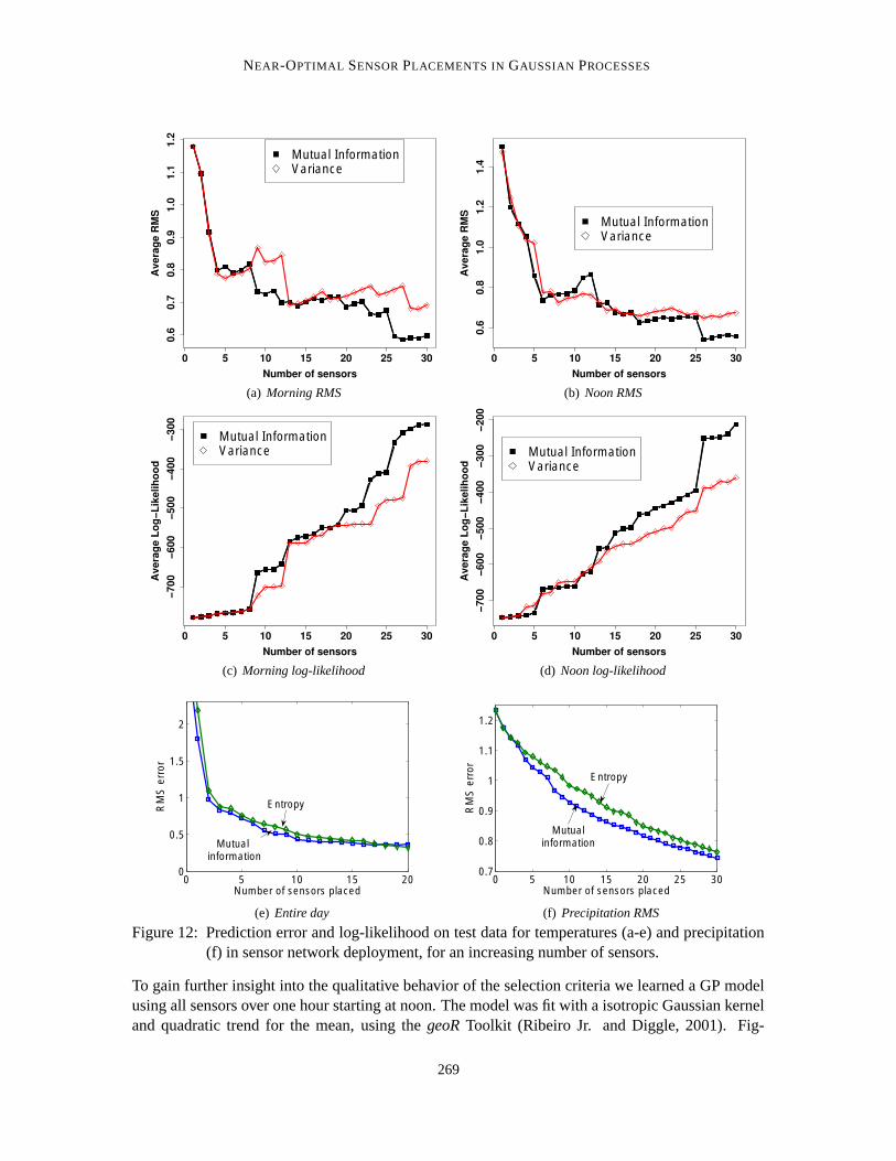
NEAR-OPTIMAL SENSOR PLACEMENTS IN GAUSSIAN PROCESSES
0 5 1 0 1 5 2 0 2 5 3 0
0.6
0.7
0.8
0.9
1.0
1.1
1.2
N u m b e r o f s e n s o r s
Av
era
ge
RM
SMutual InformationV arianc e
(a) Morning RMS
0 5 1 0 1 5 2 0 2 5 3 0
0.6
0.8
1.0
1.2
1.4
N u m b e r o f s e n s o r s
Av
era
ge
RM
S
Mutual InformationV arianc e
(b) Noon RMS
0 5 1 0 1 5 2 0 2 5 3 0
−7
00
−6
00
−5
00
−4
00
−3
00
N u m b e r o f s e n s o r s
Av
era
ge
Lo
g−
Lik
eli
ho
od
Mutual InformationV arianc e
(c) Morning log-likelihood
0 5 1 0 1 5 2 0 2 5 3 0
−7
00
−6
00
−5
00
−4
00
−3
00
−2
00
N u m b e r o f s e n s o r s
Av
era
ge
Lo
g−
Lik
eli
ho
od
Mutual InformationV arianc e
(d) Noon log-likelihood
0 5 10 15 200
0.5
1
1.5
2
Number of sensors placed
RM
S e
rror
Mutualinformation
Entropy
(e) Entire day
0 5 10 15 20 25 300.7
0.8
0.9
1
1.1
1.2
Number of sensors placed
RM
S e
rror
Entropy
Mutualinformation
(f) Precipitation RMS
Figure 12: Prediction error and log-likelihood on test data for temperatures (a-e) and precipitation(f) in sensor network deployment, for an increasing number of sensors.
To gain further insight into the qualitative behavior of the selection criteria we learned a GP modelusing all sensors over one hour starting at noon. The model was fit with a isotropic Gaussian kerneland quadratic trend for the mean, using the geoR Toolkit (Ribeiro Jr. and Diggle, 2001). Fig-
269

KRAUSE, SINGH AND GUESTRIN
ures 13(a) and 13(b) show the posterior mean and variance for the model. Using our algorithms,22 sensors were chosen using the entropy and mutual information criteria. For each set of selectedsensors, additional models were trained using only the measurements of the selected sensors. Pre-dicted temperature surfaces for the entropy and mutual information configurations are presented inFigures 13(c) and 13(d). Entropy tends to favor placing sensors near the boundary as observed inSection 3, while mutual information tends to place the sensors on the top and bottom sides, whichexhibited the most complexity and should have a higher sensor density. The predicted variances foreach model are shown in figures 13(e) and 13(f). The mutual information version has significantlylower variance than the entropy version almost everywhere, displaying, as expected, higher variancein the unsensed areas in the center of the lab.
9.5 Comparison of Mutual Information with Classical Experimental Design Criteria
In order to compare the mutual information placements with the classical optimality criteria, weperformed the following experiment. We uniformly selected 12 target locations U in the lab aslocations of interest. We then set up the linear model
xS = ΣSUΣ−1UU xU +w.
Hereby, xS denotes measurements at the locations S , among which we choose our placement, xUare the values at the locations of interest (no sensors can be placed there), and w models independentnormal measurement noise with constant variance. After subtraction of the training set mean, thismodel uses the Best Linear Unbiased (Kriging) estimator for predicting xS from xU .
The problem becomes to select the sensor locations A ⊂ S which allow most precise predictionof the variables of interest, in the sense of minimizing the error covariance 1
σ2 (AT A)−1, where A =
ΣSUΣ−1UU . The different classical design criteria vary in how the scalarization of the error covariance
is done. D-optimal design minimizes the log-determinant, A-optimal design minimizes the trace,and E-optimal design minimizes the spectral radius (the magnitude of the largest eigenvalue) of theerror covariance. Note that this problem formulation favors the classical design criteria, which aretailored to minimize the error of predicting the values at the target locations U, whereas mutualinformation and entropy just try to decrease the uncertainty in the entire space.
In order to solve the classical experimental design problems, we use the formulations as a semidef-inite program (SDP) as discussed by Boyd and Vandenberghe (2004). We use SeDuMi (Sturm,1999) for solving these SDPs. Since the integral optimization is hard, we solve the SDP relaxationto achieve a fractional design. This fractional solution defines the best way to distribute an infinite(or very large) budget of experiments to the different choices on the design menu (the variables inS ). In the sensor selection problem however, we have to solve the integral problem, since we facethe binary decision of whether a sensor should be placed at a particular location or not. This is ahard combinatorial optimization problem. Since no near-optimal solution is known, we select thelocations corresponding to the top k coefficients of the design menu, as is common practice. Wecompare the placements using the classical design criteria to those using the mutual informationand entropy criteria, and evaluate each of them on the RMS prediction accuracy on the hold-outlocations U.
270

NEAR-OPTIMAL SENSOR PLACEMENTS IN GAUSSIAN PROCESSES
0
1 0
2 0
3 0
0
1 0
2 0
3 0
4 02 1
2 2
2 3
2 4
2 5
2 6
(a) Isotropic model
0
1 0
2 0
3 0
0
1 0
2 0
3 0
4 00
0. 1
0. 2
0. 3
0. 4
0. 5
(b) Predicted variance
0
1 0
2 0
3 0
0
1 0
2 0
3 0
4 02 1
2 2
2 3
2 4
2 5
2 6
(c) Temperature (entropy)
0
1 0
2 0
3 0
0
1 0
2 0
3 0
4 02 1
2 2
2 3
2 4
2 5
2 6
(d) Temperature (mutual inf.)
0
1 0
2 0
3 0
0
1 0
2 0
3 0
4 00
0. 1
0. 2
0. 3
0. 4
0. 5
(e) Variance (entropy)
0
1 0
2 0
3 0
0
1 0
2 0
3 0
4 00
0. 1
0. 2
0. 3
0. 4
0. 5
(f) Variance (MI)
Figure 13: Comparison of predictive quality of subsets selected using MI and entropy.
Figure 14(a) presents the results of this experiment on the temperature data. We can see that eventhough mutual information optimizes for prediction accuracy in the entire space and not specificallyfor the target locations U, it incurs the least RMS prediction error, apart from the placements con-sisting only of a single sensor. E-optimal design performs comparably with the entropy criterion,and D- and A-optimality perform worse.
271

KRAUSE, SINGH AND GUESTRIN
0 2 4 6 8 100
0.5
1
1.5
2
2.5
3
3.5
Number of sensors placed
RM
S e
rror
on
targ
et
Mutualinformation Entropy
E−optimaldesign
A−optimaldesign
D−optimaldesign
(a) Comparison with A-, D- and E-optimality on temper-ature data
0 5 10 15 20 25 300.8
0.9
1
1.1
1.2
1.3
Number of sensors placed
RM
S e
rror
on
targ
et
Mutualinformation
EntropyE−optimal
design
A−optimaldesign
D−optimaldesign
(b) Comparison with A-, D- and E-optimality on precip-itation data, 111 node subsample
0 5 10 15 20 25 30
0.8
0.9
1
1.1
1.2
Number of sensors placed
RM
S e
rror
on
targ
et
Mutualinformation
Entropy
E−optimaldesign
D−optimaldesign
(c) Comparison with D- and E-optimality on precipita-tion data
MI MI loc. H A D E0
50
100
150
200
Run
ning
tim
e (s
)
(d) Running time for 111 node precipitation subsample
Figure 14: Comparison with classical experimental design. We plot RMS prediction error on 25%hold out target locations U.
When we performed the same experiment with the precipitation data, SeDuMi ran out of memory (1GB) for the SDP required to solve the A-optimality criterion. The largest subsample we could solvefor all A-, D- and E-optimality on this data set was limited to 111 locations. Figure 14(b) presents theresults. For the entire data set of 167 locations, we could still solve the D- and E-optimality SDPs.The results are presented in Figure 14(c). We can observe that for the 111 locations, D-optimalityslightly outperforms mutual information. We have to consider, however, that the classical criteriaare optimized to minimize the error covariance with respect to the locations U of interest, whereasmutual information merely tries to achieve uniformly low uncertainty over the entire space. For thefull set of 167 locations, mutual information outperforms the other design criteria.
Figure 14(d) presents the running time for optimizing A-, D-, E-optimality, and mutual information,mutual information with truncation parameter ε = 1 and entropy on the 111 node subsample of theprecipitation data on a Pentium M 1.7 GHz processor. We can see that optimizing entropy is fastest,closely followed by the truncated mutual information criterion described in Section 5.2 that is fur-ther evaluated in Section 9.7. Even without truncation, optimizing mutual information is three timesfaster than (fractionally) optimizing D-optimality and 24 times faster than A-optimality.
272

NEAR-OPTIMAL SENSOR PLACEMENTS IN GAUSSIAN PROCESSES
randomme an
randommax imu m
random+P E , max .
g re e dy +P E
g re e dyh e u ris t ic
10.0
10.5
11.0
11.5
12.0
12.5
(a) Objective values
0 5 1 0 1 5 2 0 2 5 3 0
46
810
12
N u m b e r o f s e n s o r s
Mu
tual in
form
ati
on
Greedy heuristicM a x im um o f 1 0 0 ra n do m tria lsM ea n o f 1 0 0 ra n do m tria ls
(b) Comparison of heuristics
Figure 15: Comparison of the greedy algorithm with several heuristics.
9.6 Empirical Analysis of the Greedy Algorithm
To study the effectiveness of the greedy algorithm, we compared the mutual information of the setsselected by our greedy algorithm to random selections, to a hill climbing method that uses a pairwiseexchange heuristic, and—for small subsamples—to the bounds proved by the MIP as discussed inSection 4.5.
In this experiment, we used the empirical covariance matrix as the input to the algorithms. Fig-ure 15(b) shows that the greedy algorithm provided significantly better results than the randomselections, and even the maximum of a hundred random placements did not reach the quality of thegreedy placements. Furthermore, we enhanced the random and greedy selections with the pairwiseexchange (PE) heuristic, which iteratively finds exchanges of elements y ∈ A and y′ ∈ S \A suchthat exchanging y and y′ improves the mutual information score. Figure 15(a) presents objectivevalues of these enhanced selection methods for a subset size of 12, for which the maximum over100 random selections enhanced with PE actually exceeded the greedy score (unlike with mostother subset sizes, where random + PE did about as well as the greedy algorithm). Typically, theobjective values of random + PE, greedy + PE and greedy did not differ much. Note that as men-tioned in Section 4, the performance guarantee for the greedy algorithm always provides an onlineapproximation guarantee for the other heuristics.
For a 16 node subsample of the temperature data set, we used the MIP from Section 4.5 to computebounds on the optimal mutual information. Figure 5 presents the results. It can be seen, that for thissmall subsample, the greedy solution is never more than 5 percent away from the optimal solution,which is a much tighter bound than the a priori approximation factor of (1−1/e).
We also experimented with the lazy evaluation strategy discussed in Section 5.1. For examplewhen picking placements of size 50 for the precipitation data set, the number of mutual informa-tion computations decreased from 7125 to 1172, and the computation time on a Pentium M 1.7GHz processor decreased from 41.3 seconds to 8.7 seconds. The results for both temperature andprecipitation data sets are presented in Figures 16(a) and 16(b).
273

KRAUSE, SINGH AND GUESTRIN
0 5 10 15 200
200
400
600
800
1000
Number of sensors placed
Mut
ual i
nfor
mat
ion
com
puta
tions
Standard greedy algorithm
Greedy usinglazy evaluations
(a) Temperature data
0 20 40 600
2000
4000
6000
8000
10000
Number of sensors placed
Mut
ual i
nfor
mat
ion
com
puta
tions
Standard greedy algorithm
Greedy usinglazy evaluations
(b) Precipitation data
Figure 16: Performance improvements by using lazy evaluations of mutual information.
0.0 0.5 1 .0 1 .5 2 .0 2 .5 3 .0
15
20
25
30
35
40
45
50
T r u n c a tio n p a r a m e te r
Tim
e (
seco
nd
s)
(a) Running time
0.0 0.5 1 .0 1 .5 2 .0 2 .5 3 .0
0.9
00.9
51.0
01.0
51.1
01.1
5
T r u n c a tio n p a r a m e te r
Avera
ge R
MS
(b) Approximation error
Figure 17: Analysis of the experiments with local kernels. (a) running times for increasing level oftruncation. (b) increase of average RMS error with increasing level of truncation. Notethat for a truncation between 0.5 and 1.2, a good tradeoff between running time anderror is achieved.
9.7 Results on Local Kernels
We also performed experiments to assess the running time versus quality trade-off incurred by usingapproximate local kernels. To provide intuition about the covariance structure, note that the 25, 50and 75 percentiles of the absolute covariance entries were 0.122, 0.263 and 0.442, the maximumwas 3.51, the minimum was 8.78E−6. For the variance (the diagonal entries), the median was1.70, and the minimum was 0.990. Figure 17(a) shows that the computation time can be drasticallydecreased as we increase the truncation parameter ε from 0 to the maximum variance. Figure 17(b)shows the RMS prediction accuracy for the 20 element subsets selected by Algorithm 3. Accordingto the graphs, the range ε ∈ [0.5,1] seems to provide the appropriate trade-off between computationtime and prediction accuracy.
In order to study the effect of local kernels on the placements, we performed the following ex-periment. We created a regular 7 by 7 grid with unit distance between neighboring grid points,and generated covariance matrices using two different GPs, one using the Gaussian (squared ex-ponential) kernel, and the other using the local kernel (Equation 9). We exponentially increasedthe bandwidth in eight steps from 0.1 to 12.8. Figures 18 and 19 show the corresponding place-
274

NEAR-OPTIMAL SENSOR PLACEMENTS IN GAUSSIAN PROCESSES
ments using mutual information to select the locations. From this experiment, we can see that theplacements obtained using the non-local Gaussian kernel tend to be spread out slightly more, as onemight expect. Overall, however, the placements appear to be very similar. In light of the compu-tational advantages provided by local kernels, these results provide further evidence in the spirit ofSection 9.7, namely that local kernels can be a valuable tool for developing efficient model-basedsensor placement algorithms.
2 4 61
2
3
4
5
6
7
1
2
3
4
5
6
7
8
9
Parameter 0.10
2 4 61
2
3
4
5
6
7
1
2
3
4
5
6
7
8
9
Parameter 0.20
2 4 61
2
3
4
5
6
7
1
2
3
4
5
6
7
8
9
Parameter 0.40
2 4 61
2
3
4
5
6
7
1
2
3
4
5
6
7
8
9
Parameter 0.80
2 4 61
2
3
4
5
6
7
1
2 3
4
5
6
7 8
9Parameter 1.60
2 4 61
2
3
4
5
6
7
1 2
3
4
5
6
7 8
9
Parameter 3.20
2 4 61
2
3
4
5
6
7
1
2
3
4
5 6
7
8
9Parameter 6.40
2 4 61
2
3
4
5
6
7
1
2
3
4
5
6
7 8
9
Parameter 12.80
Figure 18: Placements under Gaussian kernel, mutual information criterion, increasing bandwidth
10. Future Work
There are several interesting possible extensions to the present work. Since the predictive variance in(2) does not depend on the actual observations, any closed-loop strategy which sequentially decideson the next location to measure, surprisingly, is equivalent to an open loop placement strategy whichselects locations to make observations independently of the measured values. If there is uncertaintyabout the model parameters however, such as about the kernel bandwidths, then this is no longertrue. In this case, we expect a sequential, closed-loop strategy to be more effective for predictingspatial phenomena. Krause and Guestrin (2007) present bounds comparing the performance of theoptimal sequential strategy with the optimal fixed placement. This bound essentially depends on the
275

KRAUSE, SINGH AND GUESTRIN
2 4 61
2
3
4
5
6
7
1
2
3
4
5
6
7
8
9
Parameter 0.10
2 4 61
2
3
4
5
6
7
1
2
3
4
5
6
7
8
9
Parameter 0.20
2 4 61
2
3
4
5
6
7
1
2
3
4
5
6
7
8
9
Parameter 0.40
2 4 61
2
3
4
5
6
7
1
2
3
4
5
6
7
8
9
Parameter 0.80
2 4 61
2
3
4
5
6
7
1
2
3
4
5 6
7
8
9
Parameter 1.60
2 4 61
2
3
4
5
6
7
1
2
3
4
5
6
7
8 9
Parameter 3.20
2 4 61
2
3
4
5
6
7
1
2
3 4
5
6 7
8
9
Parameter 6.40
2 4 61
2
3
4
5
6
7
1
2 3
4 5
6 7
8
9Parameter 12.80
Figure 19: Placements under local kernel, mutual information criterion, increasing bandwidth
parameter entropy. We consider several exploration strategies for effectively reducing this parameterentropy and present sample complexity bounds. However, more work is needed in this area.
Another interesting open question is whether an approximation algorithm can be found for optimiz-ing sensor placements subject to submodular cost functions—usually, the more sensors we have tobuy, the cheaper they become per unit. To address this problem, Narasimhan and Bilmes (2006)present a submodular-supermodular procedure for bicriteria-optimization of a submodular functionof which a submodular cost is subtracted. This procedure, while elegant, unfortunately can notprovide approximation guarantees for this problem.
Of further interest are also constrained sensor placement problems, in which, for example, the placedsensors have to be connected in a routing tree, or have to lie on a collection of paths. Krause et al.(2006) provide evidence that submodularity can be leveraged to derive approximation algorithmsfor sensor placement even in these combinatorially even more challenging constrained optimizationproblems. However, there are still many open issues subject to further research.
276
NEAR-OPTIMAL SENSOR PLACEMENTS IN GAUSSIAN PROCESSES
11. Conclusions
In this paper, we tackle the problem of maximizing mutual information in order to optimize sen-sor placements. We prove that the exact optimization of mutual information is NP-complete, andprovide an approximation algorithm that is within (1− 1/e) of the maximum mutual informationconfiguration by exploiting the submodularity in the criterion. We also illustrate that submodularitycan be used to obtain online bounds, which are useful for bounding the quality of the solutions ob-tained by any optimization method, and for designing branch and bound algorithms for the mutualinformation criterion. In order to scale up the application of our approach, show how to exploitlazy evaluations and local structure in GPs to provide significant speed-ups. We also extend oursubmodularity-based analysis of mutual information to incorporate robustness to sensor failuresand model uncertainty.
Our very extensive empirical results indicate that data-driven placements can significantly improvethe prediction accuracy over geometric models. We find, in contrast to previous work (Caseltonet al., 1992; Zidek et al., 2000), that the mutual information criterion is often better than entropyand other classical experimental design criteria, both qualitatively and in prediction accuracy. Inaddition, the results show that a simple greedy algorithm for optimizing mutual information providesperformance that is very close to the optimal solution in problems that are small enough to be solvedexactly, and comparable to more complex heuristics in large problems.
We believe this work can be used to increase the efficacy of monitoring systems, and is a steptowards well-founded active learning algorithms for spatial and structured data.
Acknowledgments
We would like to thank the Action Editor (Chris Williams) and the anonymous referees for theirvaluable comments and suggestions on this work. This work was partially supported by NSF GrantNos. CNS-0509383, CNS-0625518 and a gift from Intel Corporation. Carlos Guestrin was partlysupported by an Alfred P. Sloan Fellowship and an IBM Faculty Fellowship. Andreas Krause waspartly supported by a Microsoft Research Graduate Fellowship. Ajit Singh acknowledges the sup-port of NSERC.
Appendix A. Proofs
Proof [Theorem 2] Our reduction builds on the proof by Ko et al. (1995), who show that for anygraph G, there exists a polynomially related, symmetric positive-definite matrix Σ such that Σ hasa subdeterminant (of a submatrix resulting from the selection of k rows and columns i1, . . . , ik)greater than some M if G has a clique of size at least k, and Σ does not have a subdeterminantgreater than M− ε for some (polynomially-large) ε > 0 if G does not have such a clique. LetG be a graph, and let Σ be the matrix constructed in Ko et al. (1995). We will consider Σ asthe covariance matrix of a multivariate Gaussian distribution with variables XU = {X1, . . . ,Xn}.Introduce additional variables XS = {y1, . . . ,yn} such that yi|Xi = x ∼N (x,σ2). Note that a subset
277

KRAUSE, SINGH AND GUESTRIN
A ⊆ S , |A | = k, has maximum entropy of all such subsets if and only if the parents ΓA ⊂ Uof A have maximum entropy among all such subsets of U. Now note that I(A ;(U ∪ S) \A) =H(A)−H(A | (U ∪S)\A) = H(A)−H(A |U), because yi and y j are conditionally independentgiven U. Furthermore, again because of independence, H(A |U) is a constant only depending onthe cardinality of A . Assume we could decide efficiently whether there is a subset A ⊂ S such thatI(A ;V \A)≥M′. If we choose σ2 small enough, then this would allow us to decide whether G hasa clique of size k, utilizing the gap ε.
Proof [Lemma 5] Define K (x,y) = K (x,y) for x 6= y and K (x,x) = K (x,x) + σ2 to include thesensor noise σ2. Since C is compact and K continuous, K is uniformly continuous over C . Hence,for any ε1, there exists a δ1 such that for all x,x′,y,y′,‖x− x′‖2 ≤ δ1,‖y− y′‖2 ≤ δ1 it holds that|K (x,y)−K (x′,y′)| ≤ ε1. Assume C1 ⊂ C is a finite mesh grid with mesh width 2δ1. We allowsensor placement only on grid C1. Let C2 ⊂ C be a mesh grid of mesh width 2δ1, which is derivedby translating C1 by δ1 in Euclidean norm, and let G1,G2 denote the restriction of the GP G toC1,C2. We assume C1,C2 cover C in the sense of compactness. We use the notation · to refer to thetranslated version in G2 of the random variable · in G1. K is a symmetric strictly positive definitecovariance function and |K (X ,y)− K (X , y)| ≤ ε1 for all X ,y ∈ G1. Moreover, since K is positivesemidefinite, the smallest eigenvalue of any covariance matrix derived from K is at least σ2.
Let A be a subset of C1 and X ∈ C1 \A . Using (5), we first consider the conditional variance σ2X |A .
By definition, ‖y− y‖2 ≤ δ1, and hence |K (X ,y)− K (X , y)| ≤ ε1 for all y ∈ A . Hence we knowthat ‖ΣAA −ΣAA‖2 ≤ ‖ΣAA −ΣAA‖F ≤ k2ε1. We furthermore note that ‖Σ−1
AA‖2 = λmax(Σ−1AA) =
λmin(ΣAA)−1 ≤ σ−2, and hence
‖Σ−1AA −Σ−1
AA‖2 = ‖Σ−1AA(ΣAA −ΣAA)Σ−1
AA‖2
≤ ‖Σ−1AA‖2‖ΣAA −ΣAA‖2‖Σ−1
AA‖2 ≤ σ−4k2ε1.
We derive ‖ΣXA −ΣXA‖2 ≤ ‖ε11T‖2 = ε1√
k, hence
|σ2X |A−σ2
X |A |= |ΣXA Σ−1AA ΣAX −ΣXAΣ−1
AA ΣAX |≤ 2‖ΣXA −ΣXA‖2‖Σ−1
AA‖2‖ΣXA‖2 +‖Σ−1AA −Σ−1
AA‖2‖ΣXA‖22 +O(ε2
1)
≤ 2ε1
√kσ−2M
√k +σ−4k2ε1M2k +O(ε2
1)
≤ ε1kσ−2M(2+σ−2k2M
)+O(ε2
1),
where M = maxx∈C K (x,x). We choose δ such that the above difference is bounded by σ2ε. Wenote that (assuming w.l.o.g. H(X | A)≥ H(X | A))
H(X | A)−H(X | A)=12
logσ2
X |Aσ2
X |A≤ log(1+ε)
2≤ ε
2.
which concludes the argument.
Proof [Corollary 6] The higher order terms O(ε21) can be worked out as kσ−2ε2(1 + Mk2σ−2 +
εk2σ−2). Assuming that ε < min(M,1), this is bounded by 3k3Mσ−4ε. Using the Lipschitz as-sumption, we can directly compute δ1 from ε1 in the above proof, by letting δ = ε1/L. Let R =
278

NEAR-OPTIMAL SENSOR PLACEMENTS IN GAUSSIAN PROCESSES
kσ−2M(2+σ−2k2M
)+ 3k3Mσ−4. We want to choose δ such that ε1R ≤ σ2ε. Hence if we choose
δ ≤ σ2εLR , then |H(X | A)−H(X | A)| ≤ ε uniformly as required. Note that in order to apply the
result from Nemhauser et al. (1978), the approximate monotonicity has to be guaranteed for subsetsof size 2k, which results in the stated bound.
Proof [Theorem 7] The following proof is an extension of the proof by Nemhauser et al. (1978),using some simplifications by Jon Kleinberg.
Let s1, . . . ,sk be the locations selected by the greedy algorithm. Let Ai = {s1, . . . ,si}, A∗ be theoptimal solution, and δi = MI(Ai)−MI(Ai−1). By Lemma 5, we have, for all 1≤ i≤ k,
MI(Ai∪A∗)≥MI(A∗)− kε.
We also have, for 0≤ i < k,
MI(Ai∪A∗)≤MI(Ai)+ kδi+1 =i
∑j=1
δ j + kδi+1.
Hence we have the following sequence of inequalities:
MI(A∗)− kε≤ kδ1
MI(A∗)− kε≤ δ1 + kδ2
...
MI(A∗)− kε≤k−1
∑j=1
δ j + kδk.
Now we multiply both sides of the i-th inequality by(1− 1
k
)k−1, and add all inequalities up. After
cancellation, we get(
k−1
∑i=0
(1−1/k)i
)(MI(A∗)− kε)≤ k
k
∑i=1
δi = k MI(Ak).
Hence, as claimed, with AG = Ak (i.e., AG is the k-element greedy solution)
MI(AG)≥(
1− (1−1/k)k)
(MI(A∗)− kε)≥ (1−1/e)(MI(A∗)− kε).
Proof [Remark 12] We have that H(y | Z) < 0⇔ K (y,y)+ σ2− K (Z,y)2
K (Z,Z)+σ2 < 12πe . Using a similar
argument as the proof of Lemma 5, for very fine discretizations, there exists a y arbitrarily close toZ, such that for any α > 0, |K (Z,Z)−K (y,y)| ≤ α and |K (Z,Z)−K (Z,y)| ≤ α. Plugging thesebounds into the definition of H(y | Z) and some algebraic manipulation proves the claim.
279

KRAUSE, SINGH AND GUESTRIN
References
A. C. Atkinson. Recent developments in the methods of optimum and related experimental designs.International Statistical Review / Revue Internationale de Statistique, 56(2):99–115, Aug. 1988.
A. C. Atkinson. The usefulness of optimum experimental designs. Journal of the Royal StatisticalSociety. Series B (Methodological), 58(1):59–76, 1996.
S. Axelrod, S. Fine, R. Gilad-Bachrach, R. Mendelson, and N. Tishby. The information of obser-vations and application for active learning with uncertainty. Technical report, Jerusalem: LeibnizCenter, Hebrew University, 2001.
X. Bai, S. Kumar, Z. Yun, D. Xuan, and T. H. Lai. Deploying wireless sensors to achieve bothcoverage and connectivity. In ACM International Symposium on Mobile Ad Hoc Networking andComputing, Florence, Italy, 2006.
J. M. Bernardo. Expected information as expected utility. Annals of Statistics, 7(3):686–690, May1979.
S. Boyd and L. Vandenberghe. Convex Optimization. Cambridge UP, March 2004.
W. F. Caselton and T. Hussain. Hydrologic networks: Information transmission. Journal of WaterResources Planning and Management, WR2:503–520, 1980.
W. F. Caselton and J. V. Zidek. Optimal monitoring network designs. Statistics and ProbabilityLetters, 2(4):223–227, 1984.
W. F. Caselton, L. Kan, and J. V. Zidek. Statistics in the Environmental and Earth Sciences, chapterQuality data networks that minimize entropy, pages 10–38. Halsted Press, 1992.
K. Chaloner and I. Verdinelli. Bayesian experimental design: A review. Statistical Science, 10(3):273–304, Aug. 1995. ISSN 08834237.
D. A. Cohn. Neural network exploration using optimal experiment design. In Jack D. Cowan, GeraldTesauro, and Joshua Alspector, editors, Advances in Neural Information Processing Systems,volume 6, pages 679–686. Morgan Kaufmann Publishers, Inc., 1994.
R. D. Cook and C. J. Nachtsheim. A comparison of algorithms for constructing exact D-optimaldesigns. Technometrics, 22(3):315–324, Aug. 1980. ISSN 00401706.
T. M. Cover and J. A. Thomas. Elements of Information Theory. Wiley Interscience, 1991.
N. A. C. Cressie. Statistics for Spatial Data. Wiley, 1991.
C. Currin, T. Mitchell, M. Morris, and D. Ylvisaker. Bayesian prediction of deterministic functions,with applications to the design and analysis of computer experiments. Journal of the AmericanStatistical Association, 86(416):953–963, 1991.
A. Das and D. Kempe. Algorithms for subset selection in linear regression. In Symposium on theTheory of Computing, 2008.
280

NEAR-OPTIMAL SENSOR PLACEMENTS IN GAUSSIAN PROCESSES
A. Deshpande, C. Guestrin, S. Madden, J. Hellerstein, and W. Hong. Model-driven data acquisitionin sensor networks. In Proceedings of the Thirtieth International Conference on Very Large DataBases (VLDB), 2004.
V. Federov and W. Mueller. Comparison of two approaches in the optimal design of an observationnetwork. Statistics, 20:339–351, 1989.
V. V. Fedorov. Theory of Optimal Experiments. Academic Press, 1972. Trans. W. J. Studden and E.M. Klimko.
P. Flaherty, M. Jordan, and A. Arkin. Robust design of biological experiments. In Advances inNeural Information Processing Systems (NIPS) 19, 2006.
Y. Freund, H. S. Seung, E. Shamir, and N. Tishby. Selective sampling using the query by committeealgorithm. Machine Learning, 28(2-3):133–168, 1997.
G. Golub and C. Van Loan. Matrix Computations. Johns Hopkins, 1989.
H. H. Gonzalez-Banos and J. Latombe. A randomized art-gallery algorithm for sensor placement.In Proc. 17th ACM Symposium on Computational Geometry, pages 232–240, 2001.
C. Guestrin, A. Krause, and A. Singh. Near-optimal sensor placements in Gaussian processes. InMachine Learning, Proceedings of the Twenty-Second International Conference (ICML), 2005.
P. Guttorp, N. D. Le, P. D. Sampson, and J. V. Zidek. Using entropy in the redesign of an envi-ronmental monitoring network. Technical report, Department of Statistics. University of BritishColumbia., 1992. Tech. Rep. 116.
T. Hastie, R. Tibshirani, and J. H. Friedman. The Elements of Statistical Learning. Springer, 2003.
N. Heo and P. K. Varshney. Energy-efficient deployment of intelligent mobile sensor networks.IEEE Transactions on Systems, Man and Cybernetics, Part A, 35(1):78–92, 2005.
D. S. Hochbaum and W. Maas. Approximation schemes for covering and packing problems inimage processing and VLSI. Journal of the ACM, 32:130–136, 1985.
H. Hotelling. Relations between two sets of variates. Biometrika, 28(3/4):321–377, 1936.
A. Howard, M. Mataric, and G. Sukhatme. Mobile sensor network deployment using potentialfields: A distributed, scalable solution to the area coverage problem, 2002.
R. Kershner. The number of circles covering a set. American Journal of Mathematics, 61:665–671,1939.
C. Ko, J. Lee, and M. Queyranne. An exact algorithm for maximum entropy sampling. OperationsResearch, 43(4):684–691, 1995.
A. Krause and C. Guestrin. A note on the budgeted maximization of submodular functions. Tech-nical report, CMU-CALD-05-103, 2005.
A. Krause and C. Guestrin. Nonmyopic active learning of gaussian processes: An exploration–exploitation approach. In International Conference on Machine Learning, 2007.
281

KRAUSE, SINGH AND GUESTRIN
A. Krause, C. Guestrin, A. Gupta, and J. Kleinberg. Near-optimal sensor placements: Maximizinginformation while minimizing communication cost. In Proceedings of the Fifth InternationalSymposium on Information Processing in Sensor Networks (IPSN), 2006.
N. Lawrence, M. Seeger, and R. Herbrich. Fast sparse gaussian process methods: The informativevector machine. In Advances in Neural Information Processing Systems (NIPS) 16, 2003.
U. Lerner and R. Parr. Inference in hybrid networks: Theoretical limits and practical algorithms. InProceedings of the 17th Conference in Uncertainty in Artificial Intelligence (UAI), 2001.
D. V. Lindley. On a measure of the information provided by an experiment. Annals of MathematicalStatistics, 27:986–1005, 1956.
D. V. Lindley and A. F. M. Smith. Bayes’ estimates for the linear model. Journal of the RoyalStatistical Society, Ser. B, 34:1–18, 1972.
S. P. Luttrell. The use of transinformation in the design of data sampling schemes for inverseproblems. Inverse Problems, 1:199–218, 1985.
D. MacKay. Information-based objective functions for active data selection. Neural Computation,4(4):590–604, 1992.
D. J. C. MacKay. Information Theory, Inference, and Learning Algorithms. Cambridge UP, 2003.
G. P. McCabe. Principal variables. Technometrics, 26(2):137–144, 1984.
M. D. McKay, R. J. Beckman, and W. J. Conover. A comparison of three methods for selectingvalues of input variables in the analysis of output from a computer code. Technometrics, 21(2):239–245, May 1979.
R. K. Meyer and C. J. Nachtsheim. Constructing exact D-optimal experimental designs by simulatedannealing. American Journal of Mathematical and Management Sciences, 8(3-4):329–359, 1988.
T. J. Mitchell. An algorithm for the construction of ”D-optimal” experimental designs. Technomet-rics, 16(2):203–210, May 1974a. ISSN 00401706.
T.J. Mitchell. Computer construction of ”D-optimal” first-order designs. Technometrics, 16(2):211–220, May 1974b. ISSN 00401706.
Avidan Moghaddam, Weiss. Fast pixel/part selection with sparse eigenvectors. In InternationalConference on Computer Vision, 2007.
B. Moghaddam, Y. Weiss, and S. Avidan. Spectral bounds for sparse PCA: Exact and greedyalgorithms. In Advances in Neural Information Processing Systems (NIPS) 18, 2005.
B. Moghaddam, Y. Weiss, and S. Avidan. Generalized spectral bounds for sparse LDA. In MachineLearning, Proceedings of the Twenty-Third International Conference (ICML), 2006.
M. Narasimhan and J. Bilmes. A submodular-supermodular procedure with applications to dis-criminative structure learning. In Advances in Neural Information Processing Systems (NIPS)19, 2006.
282

NEAR-OPTIMAL SENSOR PLACEMENTS IN GAUSSIAN PROCESSES
G. Nemhauser, L. Wolsey, and M. Fisher. An analysis of the approximations for maximizing sub-modular set functions. Mathematical Programming, 14:265–294, 1978.
G. L. Nemhauser and L. A. Wolsey. Studies on Graphs and Discrete Programming, chapter Max-imizing submodular set functions: Formulations and analysis of algorithms, pages 279–301.North-Holland, 1981.
N-.K Nguyen and A. J. Miller. A review of some exchange algorithms for constructing discreteD-optimal designs. Computational Statistics and Data Analysis, 14:489–498, 1992.
D. J. Nott and W. T. M. Dunsmuir. Estimation of nonstationary spatial covariance structure.Biometrika, 89:819–829, 2002.
A. O’Hagan. Curve fitting and optimal design for prediction (with discussion). Journal of the RoyalStatistical Society, Ser. B, 40:1–42, 1978.
C. J. Paciorek. Nonstationary Gaussian Processes for Regression and Spatial Modelling. PhDthesis, Carnegie Mellon University, Pittsburgh, PA, May 2003.
L. Paninski. Asymptotic theory of information-theoretic experimental design. Neural Computation,17(7):1480–1507, 2005.
F. Pukelsheim. Information increasing orderings in experimental design theory. International Sta-tistical Review / Revue Internationale de Statistique, 55(2):203–219, Aug. 1987. ISSN 03067734.
N. Ramakrishnan, C. Bailey-Kellogg, S. Tadepalli, and V. N. Pandey. Gaussian processes for activedata mining of spatial aggregates. In SIAM Data Mining, 2005.
C. E. Rasmussen and C. K. I. Williams. Gaussian Process for Machine Learning. Adaptive Com-putation and Machine Learning. MIT Press, 2006.
P. J. Ribeiro Jr. and P. J. Diggle. geoR: A package for geostatistical analysis. R-NEWS Vol 1, No 2.ISSN 1609-3631, 2001.
T. G. Robertazzi and S. C. Schwartz. An accelerated sequential algorithm for producing D-optimaldesigns. SIAM Journal of Scientific and Statistical Computing, 10(2):341–358, March 1989.
J. Sacks, S. B. Schiller, and W. J. Welch. Designs for computer experiments. Technometrics, 31(1):41–47, Feb. 1989. ISSN 00401706.
P. Sebastiani and H. P. Wynn. Maximum entropy sampling and optimal bayesian experimentaldesign. Journal of the Royal Statistical Society, Series B, 62(1):145–157, 2000.
M. Seeger. Gaussian processes for machine learning. International Journal of Neural Systems, 14(2):69–106, 2004.
M. Seeger, C. K. I. Williams, and N. D. Lawrence. Fast forward selection to speed up sparsegaussian process regression. In Proceedings of the Ninth International Workshop on ArtificialIntelligence and Statistics (AISTATS), 2003.
283

KRAUSE, SINGH AND GUESTRIN
S. Seo, M. Wallat, T. Graepel, and K. Obermayer. Gaussian process regression: Active data selectionand test point rejection. In Proceedings of the International Joint Conference on Neural Networks(IJCNN), volume 3, pages 241–246, 2000.
M. C. Shewry and H. P. Wynn. Maximum entropy sampling. Journal of Applied Statistics, 14:165–170, 1987.
A. Singh, A. Krause, C. Guestrin, W. Kaiser, and M. Batalin. Efficient planning of informative pathsfor multiple robots. In IJCAI, 2007.
E. Snelson and Z. Ghahramani. Sparse Gaussian processes using pseudo-inputs. In Advances inNeural Information Processing Systems (NIPS) 18, 2005.
P. Sollich. Learning from minimum entropy queries in a large committee machine. Physical ReviewE, 53:R2060–R2063, 1996.
A. J. Storkey. Truncated covariance matrices and Toeplitz methods in Gaussian processes. InArtificial Neural Networks - ICANN 1999, 1999.
J. F. Sturm. Using sedumi 1.02, a matlab toolbox for optimization over symmetric cones. Optimiza-tion Methods and Software, special issue on interior-point methods, 11(12):625–653, 1999.
M. Sviridenko. A note on maximizing a submodular set function subject to knapsack constraint.Operations Research Letters, 32:41–43, 2004.
S. Toumpis and G. A. Gupta. Optimal placement of nodes in large sensor networks under a generalphysical layer model. In Proc. IEEE Communications Society Conference on Sensor and Ad HocCommunications (SECON), 2005.
W. J. Welch. Branch-and-bound search for experimental design based on D-optimality and othercriteria. Technometrics, 24(1):41–48, 1982.
M. Widmann and C. S. Bretherton. 50 km resolution daily precipitation for the pacific northwest.http://www.jisao.washington.edu/data sets/widmann/, May 1999.
S. Wu and J. V. Zidek. An entropy based review of selected NADP/NTN network sites for 1983–86.Atmospheric Environment, 26A:2089–2103, 1992.
D. Ylvisaker. A Survey of Statistical Design and Linear Models, chapter Design on random fields.North-Holland, 1975.
K. Yu, J. Bi, and V. Tresp. Active learning via transductive experimental design. In MachineLearning, Proceedings of the Twenty-Third International Conference (ICML), 2006.
Z. Zhu and M. L. Stein. Spatial sampling design for prediction with estimated parameters. Journalof Agricultural, Biological and Environmental Statistics, 11:24–49, 2006.
J. V. Zidek, W. Sun, and N. D. Le. Designing and integrating composite networks for monitoringmultivariate gaussian pollution fields. Applied Statistics, 49:63–79, 2000.
D. L. Zimmerman. Optimal network design for spatial prediction, covariance parameter estimation,and empirical prediction. Environmetrics, 17(6):635–652, 2006.
284


