NCPA Optimizations at Gemini North usingFocal Plane Sharpening

by

Jesse Ball

A Thesis Submitted to the Faculty of the

COLLEGE OF OPTICAL SCIENCES

In Partial Fulfillment of the Requirements

For the Degree of

MASTER OF SCIENCE

In the Graduate College

THE UNIVERSITY OF ARIZONA

May 5, 2016

1

STATEMENT BY AUTHOR

The thesis titled NCPA Optimizations at Gemini North using Focal PlaneSharpening prepared by Jesse Ball has been submitted in partial fulfillment ofrequirements for a master’s degree at the University of Arizona and is depositedin the University Library to be made available to borrowers under rules of theLibrary.

Brief quotations from this thesis are allowable without special permission,provided that an accurate acknowledgement of the source is made. Requests forpermission for extended quotation from or reproduction of this manuscript inwhole or in part may be granted by the head of the major department or theDean of the Graduate College when in his or her judgment the proposed use ofthe material is in the interests of scholarship. In all other instances, however,permission must be obtained from the author.

SIGNED:Jesse Ball

APPROVAL BY THESIS DIRECTOR

This thesis has been approved on the date shown below:

05 May, 2016Jose Sasian DateProfessor of Optical Sciences

2

ACKNOWLEDGEMENTS

First and foremost I give my sincere and humble gratitude to Dr. Olivier Lai,who provided both the premise for this project and steadfast, patient counselin my efforts to understand and carry out the work presented in this paper.

I would also like to thank Professor Jose Sasian for his invaluable advicethroughout the process of composing this thesis and also for his guidance in mycoursework at the University of Arizona.

Particular thanks is due as well to Dr. Chadwick Trujillo for his help withAltair, to John White for his help with characterization of Altair mechanismsand many hours of hypothesizing and discussions, to Dolores Coulson for sup-porting my many years with the distance learning program, and also to GeminiObservatory both for financial support in my education and for access to theinstruments used in this project.

Finally, I would like to thank my wife, Claudia, and son, Osai, who havegiven me confidence, encouragement, patience, and understanding throughoutmy studies at the University of Arizona.

3

Contents

1 Overview of Adaptive Optics at Gemini North 91.1 Atmospheric Turbulence and the need for Adaptive Optics . . . . 91.2 The Shack-Hartmann Wavefront Sensor . . . . . . . . . . . . . . 111.3 The NCPA Problem . . . . . . . . . . . . . . . . . . . . . . . . . 141.4 Overview of Gemini’s Telescope, NIRI, and Altair . . . . . . . . 15

1.4.1 Image Quality Problems at Gemini North Observatory . . 20

2 Correcting the NCPA 212.1 The Original Approach . . . . . . . . . . . . . . . . . . . . . . . . 212.2 Focal Plane Sharpening . . . . . . . . . . . . . . . . . . . . . . . 23

2.2.1 Parameter Space . . . . . . . . . . . . . . . . . . . . . . . 242.2.2 Image Quality . . . . . . . . . . . . . . . . . . . . . . . . 25

2.3 Algorithm Selection and Simulations . . . . . . . . . . . . . . . . 262.3.1 Simplex Method . . . . . . . . . . . . . . . . . . . . . . . 272.3.2 Step-through Method . . . . . . . . . . . . . . . . . . . . 292.3.3 Other Methods . . . . . . . . . . . . . . . . . . . . . . . . 31

3 Experimental Results and Discussion 313.1 Experimental Design . . . . . . . . . . . . . . . . . . . . . . . . . 31

3.1.1 Initializations and configurations . . . . . . . . . . . . . . 323.1.2 Coding the Algorithm(s) . . . . . . . . . . . . . . . . . . . 33

3.2 Results . . . . . . . . . . . . . . . . . . . . . . . . . . . . . . . . . 393.2.1 Simplex Routine . . . . . . . . . . . . . . . . . . . . . . . 393.2.2 Step-through Routine . . . . . . . . . . . . . . . . . . . . 413.2.3 Variation With Filter Selection . . . . . . . . . . . . . . . 43

3.3 Discussion . . . . . . . . . . . . . . . . . . . . . . . . . . . . . . . 443.3.1 Future Considerations and Improvements . . . . . . . . . 46

4 Summary 49

A Logged Comparison Data Pre- and Post-optimiztion to z37 50

B Final Offset Coefficients to Default NIRI NCPA File to z37 51

C IDL Code Exerpts 52C.1 “func” code . . . . . . . . . . . . . . . . . . . . . . . . . . . . . . 52C.2 Simplex algorithm . . . . . . . . . . . . . . . . . . . . . . . . . . 54

4

C.3 Step-through algorithm . . . . . . . . . . . . . . . . . . . . . . . 56

5

List of Figures

1 Quad-cell on a Shack-Hartman WFS. The relative intensities ofeach cell are used to calculate the centroid given a known spotdiameter. In the equations above, r

s

is the radius of the spot,I

n

are the intensities measured in each individual cell, and ⌃Iisthe total intensity measured in the quad-cell. Note that thisrelationship holds only if the displacement ", is much smallerthan the angular spot size, r

s

[8]. . . . . . . . . . . . . . . . . . . 132 Adaptive Optics and NCPA Overview . . . . . . . . . . . . . . . 163 The Gemini North telescope facility. . . . . . . . . . . . . . . . . 184 Altair internal optical layout. Altair WFS (blue) and Science

light paths (orange) are separated by the dichroic beamsplitter.The common light paths are highlighted in yellow[11]. . . . . . . 19

5 NIRI internal optical layout/ light path[10]. . . . . . . . . . . . 206 Examples of the PSF of the cal source imaged on NIRI (f/32, K-

prime) with (left) no NCPA correction and (right) the “telescope”NCPA correction made through the HRWFS. . . . . . . . . . . . 23

7 Comparison of initial PSF generated by simulation code (left) tothat of the calibration source imaged through Altair onto NIRIat f/32 in K-prime with no NCPA correction (right). . . . . . . 28

8 Simulated PSFs. (Left) Initial PSF with similar properties as wesee in the calibration source through the optics with no NCPAcorrection; Strehl ~ 0.45. (Right) final PSF after the simplexalgorithm corrected terms through z11; Strehl ~ 0.97. . . . . . . 30

9 Flow Chart for generic FPS algorithm (same concept is used forboth simplex and step-through methods). . . . . . . . . . . . . . 32

10 Example log file from the output of “func,” and IDL routine de-veloped to automate the setting of NCPA file, taking of imagewith NIRI, and analysis of that image. . . . . . . . . . . . . . . . 36

11 PSF towards the end of the longest simplex run. The Simplexroutine was converging on a local minimum that exhibited a sig-nificant trefoil pattern. . . . . . . . . . . . . . . . . . . . . . . . 40

12 A parabolic fit through 7 values of Strehl vs. z5 showed a maxi-mum at about z5 = -0.14µm (PSFs shown below plot). . . . . . . 42

13 Strehl ratio vs. NCPA correction . . . . . . . . . . . . . . . . . . 43

6

14 PSFs of the calibration source imaged in closed loops throughNIRI (f/32, K-prime) with (left) the “default” NIRI NCPA filecorrection applied and (right) the new NCPA correction, opti-mized through z37. . . . . . . . . . . . . . . . . . . . . . . . . . . 45

15 Appendix A . . . . . . . . . . . . . . . . . . . . . . . . . . . . . . 5016 “func” code (pt. 1) . . . . . . . . . . . . . . . . . . . . . . . . . . 5217 “func” code (pt. 2) . . . . . . . . . . . . . . . . . . . . . . . . . . 5318 “NcpaSimplex” procedure (part 1) . . . . . . . . . . . . . . . . . 5419 “NcpaSimplex” procedure (part 2) . . . . . . . . . . . . . . . . . 5520 “ncpastep” procedure (part 1) . . . . . . . . . . . . . . . . . . . . 5621 “ncpastep” procedure (part 2) . . . . . . . . . . . . . . . . . . . . 5722 “ncpastep” procedure (part 3) . . . . . . . . . . . . . . . . . . . . 58

List of Tables

1 Optimizations of first two (astigmatism) Zernike polynomial termsthrough three other filters. The coefficient offsets are on the or-der of those found for the K-prime filter (mostly) within 0.03µm(< �/50). . . . . . . . . . . . . . . . . . . . . . . . . . . . . . . . 44

2 Appendix B . . . . . . . . . . . . . . . . . . . . . . . . . . . . . . 51

7

AbstractNon-common path aberrations (NCPA) in an adaptive optics system

are static aberrations that appear due to the difference in optical pathbetween light arriving at the wavefront sensor (WFS) and at the sciencedetector. If the adaptive optics are calibrated to output an unaberratedwavefront, then any optics outside the path of the light arriving at theWFS inherently introduce aberrations to this corrected wavefront. NCPAcorrections calibrate the adaptive optics system such that it outputs awavefront that is inverse in phase to the aberrations introduced by thesenon-common path optics, and therefore arrives unaberrated at the sciencedetector, rather than at the output of the corrective elements.

Focal plane sharpening (FPS) is one technique used to calibrate forNCPA in adaptive optics systems. Small changes in shape to the de-formable element(s) are implemented and images are taken and analyzedfor image quality (IQ) on the science detector. This process is iterateduntil the image quality is maximized and hence the NCPA are corrected.

The work carried out as described in this paper employs two FPS tech-niques at Gemini North to attempt to mitigate up to 33% of the adaptiveoptics performance and image quality degradations currently under in-vestigation. Changes in the NCPA correction are made by varying theZernike polynomial coefficients in the closed-loop correction file for Altair(the facility adaptive optics system). As these coefficients are varied dur-ing closed-loop operation, a calibration point-source at the focal plane ofthe telescope is imaged through Altair and NIRI (the facility near-infraredimager) at f/32 in K-prime (2.12 µm). These images are analyzed to de-termine the Strehl ratio, and a parabolic fit is used to determine theappropriate coefficient correction that maximizes the Strehl ratio.

Historic calibrations of the NCPA file in Altair’s control loop were doneat night on a celestial point source, and used a separate, high-resolutionWFS (with its own inherent aberrations not common to either NIRI norAltair) to measure phase corrections directly. In this paper it is shownthat using FPS on a calibration source negates both the need to use costlytime on the night sky and the use of separate optical systems (which in-troduce their own NCPA) for analysis. An increase of 6% in Strehl ratiois achieved (an improvement over current NCPA corrections of 11%), anddiscussions of future improvements and extensions of the technique is pre-sented. Furthermore, a potentially unknown problem is uncovered in theform of high spatial frequency degradation in the PSF of the calibrationsource.

8

1 Overview of Adaptive Optics at Gemini North

A brief overview of atmospheric turbulence and adaptive optics with a Shack-Hartman wavefront sensor is presented as context for the study conducted inthis paper.

1.1 Atmospheric Turbulence and the need for AdaptiveOptics

The atmosphere distorts the propagation of light much in the same wayturbulent water does (although not so drastically). Albeit a small one, theair above the planet does have an index of refraction slightly bigger than 1(vacuum), and it varies proportionately to temperature fluctuations. Thesevariations can be modeled fairly well on local time and distance scales by the“Komolgorov-Obukhov law of turbulence” and can be expressed by both spatialand temporal index structure functions. These functions basically describe ahow turbulent atmosphere with “pockets” of various sizes (spatial component)of different temperatures, moving over time (temporal component) due to windsheer affect1 the local index of refraction. We usually assume that light froma star forms at infinity and by the time it reaches the earth’s atmosphere itswavefront can be assumed to be planar (i.e., the phase of the propagating wave isconstant over the span of a plane). As the plane wave traverses these pockets ofturbulence with varying indices of refraction, different locations on the incomingwavefront will be aberrated in different manners, naturally: in effect, the phaseover an area larger than the turbulent pockets will no longer lie on the sameplane. By the time the light reaches an observer on the ground, the incomingwavefront is no longer planar, and therefore naturally produces a “blur” whenthis light passes through an imaging system. Astronomers refer to this blur as“seeing.”

When projected to a two-dimensional plane at the aperture of the telescope,the index structure functions can be expressed as phase structure functions [2].

D

�

(�r) = 6.88(�r/r0)5/3

, where �r = ⌫̄⌧

Here, �r is a displacement vector from one point on the pupil to another,1The time it takes for temperature to vary in any given spot is much less than the time it

takes wind to push another pocket of turbulence to/ from that spot [2].

9

and can be expressed temorally in terms of the average velocity, ⌫̄, of the windsheers above the observation point, and a displacement in time, ⌧ ; which isknown as the Taylor approximation and is reflects the fact that the changes intemperature that are not dependent on wind speed are negligible. Here, r0 isknown as the Fried parameter and is a measurement of the local inhomogeneitiesin index of refraction: it represents the diameter of a circular area over which theturbulent atmosphere disrupts the phase of a wavefront by 1 radian rms. TheFried parameter is related to the air mass (or zenith angle, �), the wavelength(� = 2⇡/k), and an index structure coefficient, C2

N

, that depends on height andrepresents the strength of the local inhomogeneities.[2]

r0 ⇡0.423k

2(cos �)

�1

ˆC

2N

(h)dh��3/5

To summarize, r0 is a measurement estimate of the area over which a wave-front will be notably distorted, and C

2N

characterizes the intensity of the seeing.Similarly, a parameter ⌧0 = r0/v̄ characterizes the temporal coherence of the at-mosphere. It is both r0 and ⌧0 that determine the necessary corrections neededfor an optical system with a given entrance pupil diameter.

For large, ground-based telescopes, turbulence is a fundamental limitationof the image quality. The resolution of a diffraction-limited imaging system,↵

Rayleigh

⇡ 1.22�/D, is dependent on the diameter of the entrance pupil: thebigger the telescope, the smaller (i.e., better) the angular resolution. However,as mentioned above the Fried parameter describes the diameter of local inhomo-geneities in the index of refraction, and is on the order of 10-20 cm in most sitesdedicated to astronomical telescopes (even smaller in less stable sites). Since thediameter of a large, ground-based telescope is much larger than this, the (uncor-rected) image quality is necessarily and significantly limited by the atmosphericturbulence and is only resolved on the order of �/r0. Another way to look at itis that when turbulent cells are smaller than the entrance aperture, the blurringeffects themselves are well-resolved on short spatial (and/ or temporal) scales,causing a degradation in image quality, as the phase over the entire entrancepupil is projected to the image plane. This is why smaller telescopes are notas affected by the turbulence: the aperture of such a telescope is on the orderof (or smaller than) the coherence length of the turbulence, and therefore has arelatively constant phase over the pupil (although the resolution is now limitedby the Rayleigh criterion mentioned above).

10

Due to the high resolution of large diameter telescopes and their relative sizecompared with turbulent cells, methods to alleviate these dynamic aberrationsdue to atmospheric turbulence must be invoked. Adaptive optics have been de-veloping since the mid 1950s to do just that. In general, adaptive optics consistof some sort of rapidly deformable element (DM) that can be shaped such thatthe phase variations introduced by the turbulence are “flattened” by the shapeof the optic(s). The incoming light is imaged onto a detector which rapidly2

reads and analyzes the signal and sends demands to the deformable elementthat will shape the outgoing wavefront and deliver this “flattened” wave to ascience instrument. In effect, adaptive optics strive to cancel the effects of thevariable index of refraction due to turbulence in the atmosphere.

1.2 The Shack-Hartmann Wavefront Sensor

There are many different ways to configure an adaptive optics system, includ-ing curvature sensors, pyramid sensors, and Shack-Hartmann sensors, amongothers. Gemini North’s adaptive optics facility, Altair, uses the Shack-Hartmannconfiguration. In this configuration, incoming light passes though a deformableelement, usually consisting of a deformable mirror and a separate tip/ tilt mir-ror that handles lower-order aberrations, and is split by a dichroic element suchthat the longer (near-infrared) wavelengths are passed on to a science detectorand the shorter (visible) wavelengths are sent through an array of lenslets ata pupil plane and imaged onto a separate detector. Each lenslet images thesource from a portion of the wavefront in the pupil plane, so that the detectorsees an array of (point) images. The detector is divided into sub-apertures, agrid of boxes, that surround these point-source images. In principle, the lat-eral displacement, ", of an incoming wavefront on the focal plane (detector) isrelated to the derivative (slope) of the phase3, �, at the pupil by the followingdisplacement-slope relationship:

"

Y

⇡ �2f

d

@�

@y

2The correction process for AO systems must be on the order of or faster than the coherencetime ⌧0 over which the atmosphere distorts the phase appreciably. This is, of course, dependentboth on wavelength and wind speed, but is on the order of tens to hundreds of milliseconds.

3In the field of astronomical adaptive optics, the amplitude component is usually droppedfrom the wavefront distribution due to its negligible relative contribution to rms variations inthe wavefront through atmospheric turbulence[2].

11

"

x

⇡ �2f

d

@�

@x

,

where f and d are the focal length and diameter of the lenslet, respectively. Thisfundamental relationship simply shows that the positions of the spots on thewavefront sensor’s detector exhibit a linear relationship with respect to the phaseat the pupil. Therefore, the phase can be manipulated (working backwards) toput the spots back on their ideal centroids (a square grid of spots for a flatwavefront). This is done empirically in the case of a Shack-Hartman WFS bymeasuring the centroids and applying movements to the DM in order to movethe centroids back to their ideal position on the WFS through a process knownas wavefront reconstruction.

The centroids can be calculated in various ways on various types of detectors.In the case of Altair at Gemini North, it is determined using quad-cells. Quadcells consist of four sub-apertures on the focal plane (e.g., 4 pixels in a CCD)on which the spot of an unaberrated source lands directly in the middle: thereare one set of quad-cells in the focal plane per lenslet in the pupil, and theyare well separated both by a row and column of “guard cells” that are notread out so as to mitigate cross-talk effects[12]. The centroid offset (i.e., thedisplacement ") is then calculated using the relative intensity detected on eachof these cells (Figure 1). The main advantage of using a quad-cell detector forcentroiding is that it is extremely fast to read out and to calculate comparedwith oversampling on a normal CCD. A drawback is that the centroid is under-sampled and relies heavily upon a gain factor that is determined by the size ofthe spot, which changes due to local seeing conditions and/ or when correctingextended sources such as moons, asteroids, and galactic cores. This gain factor,in Altair, is determined and accounted for within the control loops[11].

Because of the aforementioned linear relationship, the measured centroidsin the focal plane of the lenslets, in effect, are representative of the phase inthe pupil plane and thus can be used to manipulate the DM’s shape such thatthe phase is cancelled and thus the wavefront is flattened. In practice thisphase reconstruction calculation is done by first calibrating an interaction ma-trix, C, that represents the response of the deformable mirror to movement ofits actuators (somewhat analogous to the operations on the right side of thedisplacement-slope relationships shown above). To create this matrix, voltagesare applied empirically to the actuators, a, and measurements, m, of the centroid

12

Figure 1: Quad-cell on a Shack-Hartman WFS. The relative intensities of eachcell are used to calculate the centroid given a known spot diameter. In theequations above, r

s

is the radius of the spot, I

n

are the intensities measuredin each individual cell, and ⌃Iis the total intensity measured in the quad-cell.Note that this relationship holds only if the displacement ", is much smallerthan the angular spot size, r

s

[8].

offsets are taken.

m = Ca,

Using this interaction matrix, a reconstructor matrix, R, is calculated that iseffectively the inverse (or more precisely the pseudo-inverse) of the interactionmatrix, C.

a = Rm

This reconstructor matrix then generates demands for the actuators to flat-ten the wavefront based on the measurements of (new) centroids on the WFS.Note that the interaction matrix, C, is in practice not square and hence can notbe directly inverted; thus the reconstructor R is usually derived using a singu-lar value decomposition techniques on the interaction matrix, and very smallsingular values that represent “invisible” modes (piston, waffle, etc.) are filteredout. The reconstructor matrix can then be used to interact with the real-time,quad-cell centroid measurements, m, in order to calculate the actuator offsetpositions, which are then corrected by applying voltages to the DM that sendthe spots back to their ideal position on the WFS. This wavefront reconstruc-

13

tion and correction process is iterated at a very high frequency (depending onthe closed-loop gain values, up to about a tenth of the sampling frequency) sothat the correction is being made on a time scale shorter than or equal to thelimiting time scale over which the atmospheric distortion changes appreciably(⌧0).

1.3 The NCPA Problem

Aberrations from an ideal, diffraction-limited image are not only introducedby the atmosphere, but by curvatures and alignments in the elements of opti-cal systems themselves. Although major astronomical observatories certainlydesign their systems to minimize these inherent aberrations, they cannot becompletely eliminated. Therefore, after an adaptive optics system corrects forthe atmospheric turbulence and any aberrations in its light path4, the optics be-tween the deformable element and the science detector will introduce their ownaberrations to the corrected wavefront. In adaptive optics systems, the lightpath(s) after the beam-splitter traverse distinctly separate optical elements andrepresent the “non-common path(s).” In order to “provide the best image qualitypossible from the ground for telescopes of their size5,” Gemini must attempt tominimize not only atmospheric aberrations, but also these static, non-commonpath aberrations (NCPA). One way to do this is to use the adaptive optics sys-tem to provide the science instrument with a wavefront whose phase is aberratedinversely to that introduced by its own optical system’s deterministic aberra-tions, rather than simply outputting a “flattened” wavefront from the DM. Thiscan be done by changing the ideal centroids on the WFS such that the “best”arrangement of centroids on the WFS is no longer a regular grid, but one whichrepresents lateral displacements "that correspond to the wavefront distributionthat is inverse in phase to these aberrations that are characteristic of the non-common path optics in the system. This NCPA offset, a

NCPA

, can be added tothe reconstructor as a static voltage offset in actuators.

a = Rm+ a

NCPA

4Although not discussed, it should be obvious that since we use empirical centroids, allaberrations between the source and the WFS are accounted for, and not just the atmosphericturbulence (although the turbulence certainly represents the majority).

5This is one of Gemini’s two principle performance goals when the telescopes were firstbuilt[7].

14

This is the main principle behind this project, in which the NCPA correc-tions to NIRI, Gemini North’s near infrared imaging instrument, are optimizedby inserting a static correction to the Altair control loop.

An overview of the principles from sections 1.1 through 1.3 are illustratedin Figure 2. Light from a distant point source travels through the vacuum ofspace to arrive essentially as a propagating plane wave at Earth’s atmosphere.This light then travels through turbulent cells with varying indices of refractionwhich cause parts of the wavefront to travel at varying speeds, resulting in anaberrated wavefront at the entrance pupil of the telescope (purple; common-path). These aberrations are seen through a Shack-Hartman wavefront sensoras lateral displacements on a quad-cell detector through an array of lenslets,which are converted via a reconstruction matrix into actuator displacementson a deformable mirror. Since the difference in light path through the adap-tive optics and the science instrument (blue and red, respectively; non-commonpath) introduce aberrations that are unaccounted for at the wavefront sensor,a static correction to these non-common path aberrations must be applied tothe reconstruction algorithm in order to output a wavefront that is inverse inphase to that of the combined non-common path optics such that light arrivingat the imaging plane will be fully corrected. Note that if the NCPA correctionis not applied (as in the case with the traditional Shack-Hartman configurationdiscussed in section 1.2), the light coming out of the adaptive optics system willexhibit a nearly flat wavefront which is then re-aberrated by the non-commonpath optics (black, inset).

1.4 Overview of Gemini’s Telescope, NIRI, and Altair

Before delving into the details of the experiment, a very brief overview ofthe telescope, instruments, and systems involved is presented[7].

The TelescopeThe Gemini North Observatory is located near the summit of Mauna Kea

on the Big Island of Hawai’i. It is one of two twin telescopes, the other locatedon Cerro Pachón outside of La Serena, Chile.

The primary mirror is an f/1.8 convex paraboloid that is 8.1m in diameterand coupled with 120 hydraulic actuators that sit under it, providing activecorrection both for gravitational distortion due to its own weight and for low-

15

Figure 2: Adaptive Optics and NCPA Overview

16

order optical and atmospheric aberrations. The primary mirror (along with thesecondary and tertiary mirrors) are coated with silver so as to optimize thesystem for observing at wavelengths greater than 450 nm, and especially thosein the infrared.

Light from the sky is reflected from the primary mirror to a 1.023m convexhyperbolic secondary mirror that is mounted on a support system with threevoice-coil actuators that perform fast tip/tilt corrections and focus (the wholesystem is also translatable in x/y, which helps to both align the optics and cor-rect for coma). This support system and the secondary mirror are suspended12.5 meters above the primary by 8 10 mm-wide trusses that allow some flexi-bility in the case of earthquakes or other vibrational phenomenon.

From the secondary mirror, the light is then reflected back through theannulus in the primary mirror, which is baffled by a chimney, and arrives atthe tertiary mirror known as the science fold. The science fold (SF) is a planesurface mirror that is mounted in the middle of the instrument support structure(ISS), a cube metal scaffold that houses instruments on either of its six sides.The SF directs the light to one of the instruments mounted on the ISS. TheISS is also attached to a cassegrain rotator that allow the field orientation toremain constant while the Alt/ Az mount tracks the telescope across the sky.The telescope delivers a beam to its instruments with an effective focal ratio off/16, with a plate scale at the cassegrain focus of 1.61 arc seconds/ mm. On amodule above the SF, there is probe that can be inserted right into the middleof the field that directs the light to Altair. After processing and correcting thewavefront, the light is then output to the science fold and on to an instrument.

While there are many more aspects to the observatory, these are the systemsthat will be discussed in the scope of this paper.

AltairAltair (ALTittude-conjugate Adaptive optics for the InfraRed) is Gemini

North’s adaptive optics facility. Its uniqueness comes in the “altitude-conjugate”part, which refers to the fact that the deformable mirror is (or was originally) op-tically conjugate to the turbulent layer of atmosphere 6.5 km above the ground.This feature was meant to allow, at the expense of worse ground-layer turbu-lence correction, for a much wider isoplanatic patch and therefore a wider fieldof potential guide stars on any given target. Site testing during the design phaseof Altair indicated that this layer was the most turbulent, and it was originallythought that the Gemini telescope’s unique design of the dome enclosure and

17

Figure 3: The Gemini North telescope facility.

other careful measures somewhat mitigate the effects of the ground-layer turbu-lence, and allow for this unique optical design. However, since it’s constructionand commissioning, it was determined that the ground layer is, indeed and byfar, the most significant contributor (especially from within a dome environ-ment, and a field lens has since been inserted to conjugate the system to theground layer.

The deformable mirror (DM) consists of 177 actuators that can be controlledup to 1000 times per second6 (1 kHz). There is a separate tip/ tilt mirror (TT)after the DM to take out the low-order aberrations and allow the DM morebandwidth for the higher-order corrective terms.

After the adaptive optics, a beam-splitter reflects 99% of the visible lightfrom 400 - 850 nm through a gimbal mirror (for tracking the guide star) and afield stop onto the 12x12 Shack-Hartman wavefront sensor, while passing 97%of the near infrared light from 850 nm to 2.5 um to one of the instruments viathe science fold. Everything beyond this beam splitter is considered to be in thethe non-common path. Note that there is also an alternate second light pathinside Altair, accessed through an moveable-stage fold mirror, that will put the

6As discussed briefly in sections 1.1 and 1.2, the actual closed-loop correction frequency ismore on the order of 25 Hz when guiding light in the visible spectrum due to lag times andloop gains.

18

Figure 4: Altair internal optical layout. Altair WFS (blue) and Science lightpaths (orange) are separated by the dichroic beamsplitter. The common lightpaths are highlighted in yellow[11].

visible light onto three separate wavefront sensors for using a laser beacon inthe sodium layer for an artificial guide star in conjunction with a fainter naturalguide star for lower-order corrections (tip/ tilt) along with the differential focusof the astronomical field (science) and the sodium layer (laser WFS)7.

Altair outputs the telescope’s natural f/16 beam, and also provides a flatfocal surface at the same position as the bare telescope, making it relatively“transparent” to the optical designs of the instruments.

NIRINIRI is Gemini North’s Near InfraRed Imager. Although it initially had

(somewhat limited) spectroscopic capabilities as well, two key optical compo-nents (a pickoff assembly and a focal plane mask assembly) are currently non-

7While LGS corrections are not considered as part of the scope of this experiment, theyare an important part of the adaptive optics suite and Gemini North and considerations formitigation NCPA for LGS are briefly discussed in section 3.3.1

19

Figure 5: NIRI internal optical layout/ light path[10].

functional and therefore it is only used in its capacity as a near-infrared imager.The detector is a 1024 x 1024 ALADDIN InSb array and will image in the 1-5micron range, which is perfect for use with Altair since Altair lets light longerthan about 850 nm through. While the instrument offers three cameras – f/6,f/14, and f/32 – only the two slower cameras are used with adaptive optics.In f/14 the field of view is 51x51 arc seconds (0.05”/ pix). In f/32 its about22 x 22 arc seconds (0.02”/pix) and therefore is very well sampled when usedwith Altair at near-infrared wavelengths8. NIRI offers a plethora of wide- andnarrow-band filters covering it’s entire spectrally sensitive range.

1.4.1 Image Quality Problems at Gemini North Observatory

Although Altair has been delivering exceptional imaging capabilities to itsusers since its commissioning over ten years ago, its performance is far fromideal, delivering only about a 15% strehl in average (~0.5”) seeing conditions,

8Using the Rayleigh criterion (section 1.1) wavelengths longer than 0.8µm will be resolved.This experiment uses 2.12µm and is therefore well over-sampled.

20

when it should yield about 65%[1]. It is believed that there are three main un-derlying effects that drive the image quality problems we see today: high spatialfrequency aliasing of print-through from the secondary mirror, vibrations frominstruments’ cryogenic cooler cold-head pumps, and non-common path aberra-tions. The technique of focal plane sharpening is aimed at mitigating the effectsof NCPA degradation and thereby improving the image quality delivered byAltair. According to simulations, by correcting the NCPA it was estimated thatup to about a 25-30% increase in strehl may be achieved.

2 Correcting the NCPA

The rest of this paper will focus on the work done to attempt to mitigatethe suspected residual NCPA features. As will be presented in the followingsections, the NCPA static offset was already a built-in part of the Altair controlsystem. The intention of this experiment is to both create a more effective andefficient way to calibrate this as well as to improve the image quality deliveredwith Altair. Although this experiment concentrates mainly on a single camerain a single wavelength/ filter, it is expected that this work will be easily trans-lated to other modes and instruments..

2.1 The Original Approach

Documentation concerning NCPA mitigation from Altair’s commissioning(2002-2003) is unfortunately largely lacking in both content and organization,making it somewhat difficult to understand techniques and methods used in thepast. In addition, most of the experts that performed the initial calibrationshave since moved on from the organization, creating another obstacle in figuringout how the NCPA files were initially ascertained (among other inconveniences).However, there are various weblogs[15] and web pages[5]where somewhat scat-tered information can be pieced together. Most of the code used to perform thecalibrations was written in IDL and still exists, so much of the effort in com-mencing this research was spent digging through cryptic coding and scatteredweb pages to piece together a picture of just how this was obtained and howbest to move forward. Despite the challenges, an understanding of this workwas uncovered with enough detail to both utilize pieces of it in this experimentand to determine that this technique is advantageous compared with historical

21

methods.To reconstruct the wavefront after AO corrections, the use of Gemini North’s

High Resolution Wavefront Sensor (HRWFS) was employed. The HRWFS con-sists of a Shack-Harman lenslet array with 324 elements (18 x 18) and sits atthe base of a fold mirror on the bottom of the ISS, at the cassegrain focus ofthe telescope. A star was imaged through the HRWFS at night and lateraltranslations of small stellar images within the sub apertures on the WFS detec-tor were then used to reconstruct the wavefront distribution on the HRWFS.Adjustments to the NCPA file in the control loops were then made based onthese measurements to effectively flatten the phase on the HRWFS.

This comparison gave an idea of non-common path effects between Altairand the telescope in general, as all instruments that are used with Altair sharethe optical path from Altair’s BS up to the SF. While this technique is fine toget a rough estimate, it lacks accuracy in three discernible manners: it does nottake into account the instruments’ light paths, it does takes into account theHRWFS light path (which is necessarily different from that of the instruments),and it adds elements of relative flexure and rotation since the calibration istaken while tracking a star on the night sky9. Furthermore, it uses valuable10

time on the night sky that could be used for observing science targets. Theseinaccuracies and inefficiencies drive the need for a more accurate and moreefficient method to compensate for the static NCPA. To work around the issue ofthe differences in OPD (and hence “induced” NCPA), it appears that correctionswere somehow introduced to the default NCPA file, although it is unknown howthis was ascertained, and it is entirely possible (and it is rumored to be so) thatthis was a “manual” or “by eye” intervention approach. Although somewhatcrude, this would be one “manual” manner in which to execute a focal planesharpening technique.

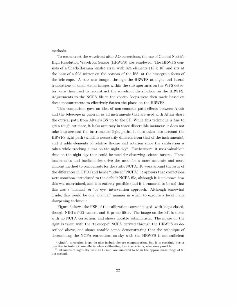
Figure 6 shows the PSF of the calibration source imaged, with loops closed,though NIRI’s f/32 camera and K-prime filter. The image on the left is takenwith no NCPA correction, and shows notable astigmatism. The image on theright is taken with the “telescope” NCPA derived through the HRWFS as de-scribed above, and shows notable coma, demonstrating that the technique ofdetermining the NCPA corrections on-sky with the HRWFS is not sufficient

9Altair’s correction loops do also include flexure compensation, but it is certainly betterpractice to isolate those effects when calibrating for other effects, whenever possible

10Estimates of night sky time at Gemini are rumored to be in the approximate range of $3per second.

22

Figure 6: Examples of the PSF of the cal source imaged on NIRI (f/32, K-prime)with (left) no NCPA correction and (right) the “telescope” NCPA correctionmade through the HRWFS.

because it both introduces aberration from the system used and does not com-pensate for aberrations for other systems. Figure 14 (left, section 3.3) shows thePSF with the “default” NIRI NCPA correction (apparently derived “by eye” asdiscussed above) and is notably better, although does still exhibit a very smallamount of 45 degree astigmatism, which is later corrected using the methodsdescribed in section 3.

2.2 Focal Plane Sharpening

Focal plane sharpening (FPS) is an empirical method of finding the NCPAby trial-and-error. The idea is to use the direct measurement of images while it-erating through changes in the shape of the deformable mirror until the sharpestimage is obtained. Once the state of the DM is known for the best image, thedifference between this state and the nominal state will directly determine thestatic offset that needs to be applied to mitigate the NCPA. Since this methodis empirical, there are countless ways to implement this in an experimental sit-uation. Some considerations in choosing a method include (but are not limitedto) accuracy, convergence time, practicality, ease of use, etc. The main advan-tage of this technique is its inherent simplicity in that results can be obtainedwithout careful regard to the characterization of the system’s properties – thisis in stark contrast with other approaches, such as phase diversity [3], which rely

23

critically on the stability and precisely known system parameters.This approach also eliminates all four of the shortcomings discussed in sec-

tion 2.1 as well as offering even further advantages. Using a calibration source(rather than a star) allows the calibrations to be carried out during the day sothat valuable time at night can be used more productively on scientific observa-tions. The calibrations are run while the telescope is stationary at the zenith,eliminating any dynamic and differential flexure contributions that would other-wise be caused by gravitational forces due to the elevation angle of the telescopeas it tracks across the sky. Furthermore, since the calibration source is mountedinside Altair, it is decoupled from potential rotational effects that the field mightotherwise contribute. Additionally, since the vibrational problems discussed insection 1.4.1 manifest most intensely at the primary mirror (m1) and the print-through/ aliasing effects originate in the secondary (m2), which are both beforethe calibration source, these two major contributions to the degradation of im-age quality are also decoupled from the NCPA correction inadequacies. Finally,the problem associated with introducing unrelated NCPA corrections from dis-tinctly different optics (namely, the HRWFS) is eliminated by measuring theimage quality directly on the detector of the instrument being optimized. Thisensures that the calibration obtained is purely related to the NCPA correctionsfor that specific instrument configuration.

Two main parameters must be selected in developing any algorithm thatwill converge on a “best” solution for the NCPA correction: parameter spaceand IQ metric. After selecting appropriate parameters, simulations are carriedout using different algorithms before actually implementing a procedure on thesystems.

2.2.1 Parameter Space

Two potential parameters, among others, for adjustments to the DM shapeinclude Zernike modes and actuators modes.

Although there are countless numbers of orthogonal bases over which couldbe chosen, the Zernike polynomials offer a natural approach across a circularpupil and are readily integrated into current software and analysis scripts11.

11Altair’s DM actually uses an “Orthonormal mirror Zernike basis” which is a projectionof the Zernike polynomials onto the deformable mirror that takes into account the centralobscuration (pinhole mirror) and the actuators and represents very well the first 12 radialorders (up to Z136) of the Zernike polynomials[18]. For the purposes of this paper, the term

24

By choosing an orthonormal basis we mitigate cross-talk between terms andensure that optimization of a single term can only increase the image quality,thereby allowing for optimization in stages. When each term can be optimizedindependently, obtaining precious telescope time becomes much more practicalsince much smaller contiguous time periods are needed, and independent resultsmay be pieced together depending on the algorithm used.

In contrast, varying actuators on the DM individually is another intriguingpotential parameter space to consider, and offers a natural approach across theactual manufactured DM since these are the finest movements that can be made.One potential advantage that this parameter may offer over using an orthonor-mal polynomial basis is that it could much more quickly converge on correctionsof aberrations that exhibit very high spatial frequencies. In a polynomial basis,these types of aberrations may not be corrected in the first handful of termsand could therefore either remain uncorrected or take an impractical amountof iterations to converge on an appropriate solution. Furthermore, this methodcould mitigate problems that may be caused by performance variance acrossthe actuators. For example, if there were an actuator that weren’t functioningat its full stroke or if it weren’t functioning at all, then using a polynomialorthonormal basis would never converge on an appropriate solution since thecorrections themselves would be inherently flawed. However, varying individualactuators could work around this by having adjacent or even opposing actuatorscompensate, since this basis is inherently not orthonormal with respect to thephase.

In researching past techniques used to mitigate NCPAs between Altair andNIRI[5], evidence of IDL code for both types of these approaches was found,although it was not apparent that the actuator space method was ever success-fully implemented.

2.2.2 Image Quality

The metric used for the solution is also quite important in influencing theeffectiveness of the technique. Since FPS is an empirical method, the accuracy towhich the correct offset to the “flattened” DM can be determine depends directlyon how accurately the image quality (IQ) on the detector can be measured. Somepotentially useful metrics include peak intensity, full width at half maximum,

“Zernike,” when used to refer to the corrections applied to the DM, refers to this basis andnot to the true Zernike polynomial.

25

encircled energy, Strehl ratio, noise equivalent area, and countless more.Peak intensity might be the most straightforward way to measure the image

quality, but it does not come without its disadvantages. For example, asym-metric (or “coma-like”) aberrations may get improperly accounted (e.g., if forinstance there were a lot of coma, but the peak of the spot was very brightdespite the offset aberration in the shape). Asymmetric aberrations could alsohave negative effects on FWHM measurements, depending on the axis throughwhich the cut(s) is(are) made. Of course, encircled energy would have similarlimitations as well. Another interesting metric to explore might be the so-called“Strehl width,” which involves comparing the image’s width to the width of auniformly illuminated disk with the same total flux and central intensity (akinto using enclosed energy)[2].

Using the Strehl ratio is a good way to avoid issues with the shape of thePSF, since it directly compares the measured peak centroid intensity with theunaberrated, diffraction limited PSF’s peak at the center and therefore won’t gettripped up by asymmetric aberrations or any other anomalous shape in the PSFthat may fool other more simple IQ metrics. Strehl is an accepted and widelyused metric in the adaptive optics community as well, so it seems like a naturallysound choice. Using Strehl ratio also makes development simpler, consideringthat much of the existing image analysis code in the Altair and NIRI librariesuse this metric as well. Using the Strehl ratio is not without its own limitations,of course. The PSF must be diffraction limited and the background must bewell characterized, or results will be inconsistent. Furthermore, the Strehl ratiomust be relatively significant in order to be accurate, so a good initial shapeof the DM must be known, and deviations from this shape must not be extreme.

2.3 Algorithm Selection and Simulations

Selection of an algorithm that explores the parameter space in terms of theimage quality metric is also a key decision in executing the FPS technique.Studies in the field of maximization can get quite complex, and practical con-siderations must be taken in order to avoid negating the some of the advantagesof using the technique. For the the investigations carried out in this work, twosimple algorithms were considered, simulated, and implemented: the well-knowndownhill simplex minimization algorithm and a simple “step-through” approach.

26

2.3.1 Simplex Method

The goal of whichever algorithm is chosen is to maximize the IQ metric asa function of the parameter space. One well-known method of minimizing afunction12 in terms of multi-dimensional parameters is called the downhill sim-plex method (also known as the “amoeba” function). If the parameter spacecontains N dimensions (independent variables), the simplex is a “shape” withN +1 points, all connected by straight lines (e.g. a triangle in two-dimensionalspace). This simplex shape converges on a minimum (although not necessarilya global minimum) by starting in some given configuration and moving one ofits extreme points (either a maximum or minimum) through a reflection, expan-sion, contraction, or combination thereof until it converges to a given fractionaltolerance. The concept is simplest to imagine in two or three dimensions, butis applicable in any number. It is not usually the most efficient way in termsof number of iterations to converge on a minimum, but it works well withouthaving to perform complicated gradients or other computationally intensive op-erations as it only has to evaluate a given function at each iterative step[4].Within IDL, the routine that executes this algorithm is known as “amoeba” andit takes a function with one input variable (in this case, a vector of Zernikecoefficients) and morphs through the variable transformations and executes thefunction one step at a time. The fractional tolerance desired for convergence isentered, along with the maximum spread, or scale, of the variables and somegiven starting point.

SimulationTo simulate the experiment using the simplex method, a randomized phase

was generated as a starting point. This was generated by adding phase contri-butions from Zernike terms through z22, each successive coefficient with mono-tonically smaller weight and such that the overall PSF held somewhat similarproperties to that of the image of the calibration source through Altair andNIRI under closed loop using no NCPA correction file (i.e., about 45% strehl,exhibiting some notable astigmatisms, as in figure 6 (left)).

Zernike polynomials out to a chosen term, j 13, were generated over a circular12Minimization and maximization are different only in semantics in that minimization al-

gorithms can be applied to the negative of an outcome in order to maximize the function.13For all purposes in this paper, the indices of the Zernike polynomials are referred to using

the so-called “Noll sequential indices,” or j such that Z1 is piston, Z2 and Z3 are tip and tilt,Z4 is focus, Z5 is primary 45 deg astigmatism, etc. [20]

27

Figure 7: Comparison of initial PSF generated by simulation code (left) to thatof the calibration source imaged through Altair onto NIRI at f/32 in K-primewith no NCPA correction (right).

disk to form a basis for the simulated phase. To construct the starting point,or initial aberrated PSF, coefficients for Zernike terms out to z22 (secondaryspherical aberration) were generated randomly using IDL’s “randomn” routine,and modified to decrease monotonically by dividing by a vector of monotonicallyincreasing integers created by the “findgen” routine in IDL. This effectively givesa random vector where each term decreases monotonically. To mimic the typicalPSF of the A-star seen with no NCPA correction in NIRI, the “findgen” factorwas taken to the power of 3/4, the randomly generated vector was multipliedby two, and the two primary astigmatism coefficients were given extra weightby a factor of 3.5. When this vector of randomly generated coefficients wasmultiplied by the vector of Zernike polynomials, and the phase contributionfrom each term was summed, it consistently produced a PSF similar to14 thatseen in the images of the Altair calibration source without NCPA correction(see Figure 7), and yielded a similar Strehl ratio between 0.4 and 0.5.

In order to simulate the NCPA correction using a downhill simplex method,the phase that gave this initial PSF was then corrected by adding a phase con-sisting of set of Zernike coefficients through z11 that varied according to the“amoeba” function in idl (i.e., the downhill simplex routine). This techniqueeffectively simulates moving the DM in Zernike space. The input function for

14While the central core of the PSFs of figure 7 are indeed similar, it is worthwhile to notethat the outer structure (i.e., the airy rings, or higher spatial frequency portions) are not atall similar. This phenomenon will be one of the main discussion points in section 3.3.

28

the amoeba routine, “func,” returned the negative of the Strehl value of a PSFgenerated by the amoeba function’s variation in the coefficients. The PSF wascalculated by taking the inverse Fourier transform of the absolute square of thepupil function, which consists of the complex vector e

i�, across the pupil15,where � is the phase generated by the sum of the Zernike polynomials and theirrespective coefficients. A “theoretical” PSF was generated the same way, butwith no additional phase introduced. The Strehl ratio is then the ratio of thenormalized maximum PSF at its center to the normalized maximum theoreticalPSF at its center. Thus the “amoeba” function was given an initial (aberrated)phase and a vector of Zernike coefficients (starting with all zeros) and outputa negative strehl ratio, minimized using the downhill simplex method. A func-tional tolerance of .001 was given to the Strehl. A weighted vector of rangeswhich again became weaker with successive terms was applied to the coefficientsso as not to stray too far from the original, decent image quality and ensureit doesn’t fall in a local minimum. Strehl ratios on the order of 90-95% wereobtained using this method, and convergence times of around 60 -120 secondswere typical.

2.3.2 Step-through Method

Since the Zernike polynomial consists of independent, orthonormal terms,a “step-through” or “focusing” method may suffice as well. In this approach,each coefficient (starting at z5, 45º astigmatism) is varied and optimized byindependently stepping through a range of values and analyzing each outcometo find a best Strehl ratio and its corresponding coefficient(s). Terms z1 - z4are omitted, as they represent piston, defocus, tip, and tilt and do not distortthe shape of the PSF in the same manner as the other terms (i.e., tip/ tilt arelateral displacements and defocus is a symmetric blurring, all of which are takeninto account by m2, rather than Altair, on the telescope).

It should also be noted that the step-through method, if proven to work, hasanother very fundamental advantage: the optimization can be done piecewisein small increments (one term at a time), rather than one single run to optimizeall coefficients. Obtaining access to the telescope, even in daytime hours, is notwithout contention and difficulty. There are always daytime maintenance tasksand other tests to be run on other instruments, etc. So having an algorithm

15A uniform apodization function was used for the pupil function: 1 inside the aperture and0 outside.

29

Figure 8: Simulated PSFs. (Left) Initial PSF with similar properties as we seein the calibration source through the optics with no NCPA correction; Strehl~ 0.45. (Right) final PSF after the simplex algorithm corrected terms throughz11; Strehl ~ 0.97.

that can be executed piecewise exhibits a real and practical advantage.

SimulationSimulations were also run on the step-through method. The same phase

initialization algorithm was used as in the downhill simplex method. This time,however, the coefficients were varied linearly through their selected range andthe Strehl ratio was measured on each step, again calculated as described inthe simplex simulation. In the simulations16, the step sizes were incrementallymade finer around the values where the maximum Strehl was found at eachcoefficient until a functional tolerance of 0.001 Strehl was met. The results ofthese simulations were indiscernible from those of the simplex method (figure8), and yielded a Strehl of over 95% when correcting out to z11.

Again, the initial phase was generated out to z22; the purpose in not correct-ing all the terms was to provide a conservative buffer for a real-world scenariowhere there may be higher-order effects than we can realistically account for.When corrected to z22, Strehl ratios of over 0.99 were obtained in both methods,

16In the actual experiment a parabolic fit was found to be just as useful as incrementallytuning the step size, due to the standard deviation of the measurements (i.e., the Strehlwas only determined to within .02, and the coefficients to within .01 µm, and thus using apolynomial fit saved a extreme amount of time).

30

and served as a sanity check that the programing was functioning as designedand expected.

2.3.3 Other Methods

The algorithms highlighted in this paper are of the very simplest sort, andit is worth mentioning that attempting other minimization techniques, such asPowell’s method or even a much more complicated approach such as the Ferretalgorithm suggested in [3], may be more efficient and effective. Approaches suchas these, and even exploring the simplex method further, may rely on the obser-vatory’s prioritization of obtaining more reliable detector control electronics, asthey certainly demand that many images be taken successively See section 3.2.1for a brief discussion on the instrument instabilities that impede such methodsat Gemini North. That being said, the maximization and minimization algo-rithms could also be adapted to not be so susceptible to electronics crashes, andbe edited such that they could pick up where they left off.

3 Experimental Results and Discussion

This section will describe the design and experimental set-up, the data col-lected and their analysis, and a discussion of the results and their meaning andsignificance in terms of improving the image quality delivered through Altair atGemini North.

3.1 Experimental Design

The experimental configuration and design and the data collection processesare presented in this section. The flowchart presented in figure 9 below showsthe generalized approach to the design of the experiment. The initializations,which include the alignment and verification procedures, are done first and theautomated procedure that was developed for this experiment follows: an im-age is taken, the image is analyzed to obtain the Strehl ratio, a new NCPAadjustment is made and implemented, and this process continues until the max-imization is reached according to the criteria set.

31

Figure 9: Flow Chart for generic FPS algorithm (same concept is used for bothsimplex and step-through methods).

3.1.1 Initializations and configurations

While the majority of the data collection was taken autonomously aftersoftware code was developed, each session had to be manually configured asdescribed below.

The telescope was moved to the zenith position and locked, and the cassegrainrotator was left parked at a random location in each session (since the field isinternal, there is no rotational dependence). Altair’s control matrix, which setsgain parameters derived from environmental data such as wind speed, r0, seeing,etc., was set to its default, as is practice when doing work with the calibrationsource.

A pinhole calibration source (known as the “A-star”, or artificial star) wasinserted near the entrance of Altair, replacing the field lens near the telescope’sfocal plan. Altair was configured in “NGS mode” such that light from the sourcetravels through the NGS light path and is imaged onto the NGS WFS for closed-loop correction. Guide loops were then closed and the A-star was imaged on

32

the NIRI detector through the K-prime filter and the f/32 camera where itsposition on the detector was ascertained. Loops were then opened and the A-star was translated towards the center of the NIRI detector. The calibrationsource was then aligned by eye on the WFS by means of a movable gimbal mirror(see Figure 4) as the WFS was read out in real time and light was distributedevenly across its sub-apertures17. This process was iterated manually until theA-star was near the center of the NIRI detector, avoiding any bad pixel patches,and also aligned on the NGS WFS. Since the positions of the steering opticsand/ or the A-star were not repeatable to a reasonable enough accuracy, thisprocedure was done at the beginning of each session. The repeatability issuesmay stem from daily calibration (and hence movement) of the Altair steeringgimbal mirrors, or may lie in the A-star/ field lens assembly mechanism, whichis also a part of the daily calibration procedures.

The NIRI configuration (f/32 camera at 2.12µm) was manually implementedusing the instrument’s EPICS dm-screen interface, and was chosen for this ex-periment for two reasons. First and foremost, it is oversampled (see section )and therefore the diffraction pattern should be easily discernible, and calculationof the Strehl ratio should therefore be accurate. Secondly, the nightly instru-ment monitoring program known at Gemini as “SV-101” is set up in the sameconfiguration to image a bright star at the beginning of each night, so there isa huge amount of data for easy comparison, especially for when the results areimplemented on-sky. The exposure time was set at 0.05s x 20 co-adds for a 1stotal integration time. In order to test the configuration, the last image takenafter the alignment was analyzed to extract a radial profile in PyRAF softwareso that it could be checked for saturation and other potentially adverse effects.Images are stored in the FITS format, which also contains header informationabout the parameters discussed above. They are stored in the Gemini Archive,and a copy of each was also moved to another personal permanent directory forease of access.

3.1.2 Coding the Algorithm(s)

IDL code was developed for this experiment that is analogous to the algo-rithms described in the sections about the simplex and step-through simulationsin section 2.3. For this development, as stated earlier, some of the more techni-

17Note that this “eyeball” alignment is just fine since the internal TT mirror, when the guideloops are closed, will correct for any small misalignment.

33

cal coding was already available in the form of IDL functions and procedures18,and this code was studied and incorporated into the algorithms designed forthis particular experiment as described below.

The “func” ProcedureA function named “func” was developed as the “heart” of the code and covers

the top three blocks in the flowchart in figure 9: applying corrections, takingthe image, and analyzing the image. The reason for the naming of the functionwas simply that the “amoeba” procedure in IDL expects this name as the func-tion it calls to work with in its minimization. “Amoeba” furthermore expectsonly one input variable. For this experiment the variable, c, was the vector ofZernike coefficients, and all other variables that passed between procedures andfunctions had to be inserted into a common block of variables rather than bedefined as a parameter of the function. A detailed description of the function“func” follows, and the code itself can bee seen in Appendix C.1.

The first thing that “func” does is open the guide loops (if they’re closed)and update the NCPA file. Loops are opened with a simple I/O routine fromthe Gemini IDL library that was modified slightly for this project. With theloops open, the NCPA file is adjusted with the addition of a vector of Zernikecoefficients – this vector will be addressed in the following paragraphs and isdefined by other procedures in the algorithm. A Gemini IDL procedure named“updateAoNcpaPar” handles converting the Zernike coefficients into the NCPAmatrix that sets the static offset on the actuators. The output of this procedureis a new NCPA file, which can then be set as the new default offset usingan IDL function developed for this project named “setncpa.” Note that thefirst iteration of “func” (depending on the procedure that calls it) usually callsa vector of zeros to the “updateAoNcpaPar” procedure and hence the NCPAoffset is not actually changed until the second iteration. Each time the NCPAfile is loaded, a control matrix has to be initialized, so a simple script called“clickCreateNewControlMatrix” was developed that simply loads the defaultcontrol matrix as discussed above. The NCPA files themselves consist of a largeand complicated matrix that is added to the reconstruction term as a static offsetin actuator voltages that correspond to a “zero point” in the spot positions onthe WFS (i.e, a

NCPA

from section 1.3). This is the file that is updated by the18Although some code already existed, documentation was rare and unclear, and a good

portion of the work on this project went into studying the old code to figure out how to hookit into these relatively simple algorithms.

34

outcome of the experiment, and there are two such files for each instrument thatis used with Altair (one for LGS and one for NGS – this project focuses on theNGS calibration).

After the NCPA file is updated and loaded, the guide loops are closed againand a wait-time of 16 seconds is begun in order to let the loop gains and correc-tions settle. The value for this wait-time was adopted from historical implemen-tations of NCPA corrections as discussed in section 2.1 and should be more thansufficient for a calibration source, since it was originally used on a stellar sourcewhich needed time to calculate seeing measurements and bandwidth to adjusttip-tilt according to local seeing variability and wind speed, etc. Between theend of this wait period and image integration, a quick check was implementedto make sure the loops were still closed and correcting due to some instabilitiesin the optimizer whereby the reconstructor would lag and loops would sponta-neously open. Although this was a relatively infrequent occurrence, it transpiredenough (and during a period of time when the experiment was unattended) towarrant the development of this extra automated check. If the reconstructorwas found to be lagging, the loops were simply commanded to re-closed andanother 16s wait-time commenced.

When the 16s wait-time and reconstructor check is done, a series of im-ages is taken on NIRI and each one is analyzed individually. The number ofimages taken is usually set during the initializations which take place in a sep-arate procedure, but can be set in “func” if no such parameter is included inthe common variable block. Due to the variability in background noise and inStrehl measurements, this number was nominally set to 10 in order to providea good sample over which to average. The procedure “goniri” was developedto simply tell the detector controller to take an image; all other parameters,such as integration time, filter, instrument configuration, etc., are set manuallyin the initialization stage described above. After one image is read out, thefile is converted to a two dimensional array in IDL using a procedure called“fits_read” from the IDL Astronomy User’s Library. The “sky” image (takenas an initialization in whichever procedure calls on “func”) is then subtractedfrom the image to remove bad/ hot pixels and give the image a zero-baseline. Afunction called “histmax” is then called to calculate the mode of the histogramwhich is used as a background measurement for the Strehl calculation19. The

19The “fwhmstrehl” routine actually does its own automated background estimation usinginterpolation of the zero-point in the MTF, but the histogram background was both found tobe very accurate and to provide a good check against the automatic background calculation

35

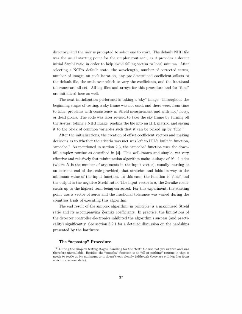
Figure 10: Example log file from the output of “func,” and IDL routine developedto automate the setting of NCPA file, taking of image with NIRI, and analysisof that image.

Strehl ratio is then calculated in a function called “fwhmstrehl,” which is alsoa part of the Gemini IDL library. It calculates the Strehl ratio by comparingthe maximum intensity of the image’s PSF, normalized by its total intensity tothe maximum of the theoretical PSF (or airy pattern) given the OTF of thesystem, normalized by its total intensity. Then, for each image in the series, the“func” routine stores the Strehl value in an array and after the last image themean value and standard deviation are calculated. Note that on each image,the “func” routine writes a log entry with data about the calculated Strehl, theZernike coefficient values, and the corresponding image name for reference. Aline with the mean Strehl and standard deviation is also included at the end ofthe output of the log file. Figure 10 shows an example of such a log file. Theresult of “func” is the negative20 of the calculated mean Strehl ratio.

The “NcpaSimplex” ProcedureAnother IDL procedure called “NcpaSimplex” was developed to fulfill the

roles of the other four blocks in the flowchart (figure 9): initializations, creationof NCPA offset vector, and criteria decision-making. This procedure first ini-tializes parameters and log files that are used in the “func” routine, then it usesa well-known minimization algorithm to vary the Zernike coefficients (via the“func” function described above) and decide if/ when the tolerance criteria ismet. This code is included in Appendix C.2.

To initialize Altair, the procedure loads all NCPA default files (includingthe NIRI, GMOS, “zero,” “telescope,” and “test” files) to the temporary IDL

in the “fwhmstrehl” procedure.20Again, this is because the “amoeba” routine minimizes its input function.

36

directory, and the user is prompted to select one to start. The default NIRI filewas the usual starting point for the simplex routine21, as it provides a decentinitial Strehl ratio in order to help avoid falling victim to local minima. Afterselecting a NCPA default state, the wavelength, number of corrected terms,number of images on each iteration, any pre-determined coefficient offsets tothe default file, the scale over which to vary the coefficients, and the fractionaltolerance are all set. All log files and arrays for this procedure and for “func”are initialized here as well.

The next initialization performed is taking a “sky” image. Throughout thebeginning stages of testing, a sky frame was not used, and there were, from timeto time, problems with consistency in Strehl measurement and with hot/ noisy,or dead pixels. The code was later revised to take the sky frame by turning offthe A-star, taking a NIRI image, reading the file into an IDL matrix, and savingit to the block of common variables such that it can be picked up by “func.”

After the initializations, the creation of offset coefficient vectors and makingdecisions as to whether the criteria was met was left to IDL’s built in function,“amoeba.” As mentioned in section 2.3, the “amoeba” function uses the down-hill simplex routine as described in [4]. This well-known and simple, yet veryeffective and relatively fast minimization algorithm makes a shape of N+1 sides(where N is the number of arguments in the input vector), usually starting atan extreme end of the scale provided) that stretches and folds its way to theminimum value of the input function. In this case, the function is “func” andthe output is the negative Strehl ratio. The input vector is a, the Zernike coeffi-cients up to the highest term being corrected. For this experiment, the startingpoint was a vector of zeros and the fractional tolerance was varied during thecountless trials of executing this algorithm.

The end result of the simplex algorithm, in principle, is a maximized Strehlratio and its accompanying Zernike coefficients. In practice, the limitations ofthe detector controller electronics inhibited the algorithm’s success (and practi-cality) significantly. See section 3.2.1 for a detailed discussion on the hardshipspresented by the hardware.

The “ncpastep” Procedure21During the simplex testing stages, handling for the “test” file was not yet written and was

therefore unavailable. Besides, the “amoeba” function is an “all-or-nothing” routine in that itneeds to settle on its minimum or it doesn’t exit cleanly (although there are still log files fromwhich to recover data).

37

The procedure written to execute the “step-through” technique was named“ncpastep.” This procedure fulfilled the same parts of the design flowchart andused many of the same initialization procedures as the “NcpaSimplex” codediscussed above, including setting initial parameters and taking a sky frame,etc. The code in its entirety can be seen in Appendix C.3.

One difference is that this procedure was aimed to alleviate the need tocomplete the optimization of every term simultaneously, so it was designed todo one coefficient per run. Therefore, the initial parameters also included settingwhich term to correct (i.e., z=5 for primary 45-deg astigmatism, z=6 for primary0-deg astigmatism, etc.), and the selection of the number of steps with which towalk through the coefficient variations (and hence by how much to vary themon each step). Also, after the first few terms in the polynomial, it becomescumbersome to enter the coefficients manually on each run, so a method to savethe output to a temporary or “test” NCPA file was devised and henceforth usedinstead of reverting to the default NIRI file on each trial.

Coding the actual procedure was relatively straightforward. The number ofsteps were input along with the range over which to vary the coefficient, andthis information gives step sizes and hence the values of the vector to input tothe “func” procedure (i.e., divide the range by the number of steps to get theinterval, start at the negative range and step through accordingly – note thata “0” value is always added and the value of the range on both the positiveand negative sides are anchored). Using the “test” NCPA file as a default input(assuming the test file has the first n Zernike coefficients already maximized),the vector, a, input to the “func” procedure to maximize the n + 1 coefficientis simply a vector of n + 1 zeros. Of course, the option to manually define thecoefficients is always available as well. Once the output of “func” was recordedand logged for each step in the range of the coefficient, a plot of Strehl vs. co-efficient value was generated and a second-order polynomial fit was producedwith IDL’s built-in “poly_fit” routine. Then the coefficient that corresponds tothe maximum value is simply where the derivative is zero (e.g., x

max

=

�b

2a ).This value is then input to the “updateAoNcpaPar” in order to be converted tothe appropriate addition in the NCPA file and saved as the new “test” file. Thisprocess is iterated as far as it is warranted, and can be done on individual termsin separate sessions, which not only eludes hardware issues related to length ofuse or number of images taken, but also allows the procedure to be done justabout any time the telescope is free for 30 min or more throughout the day,whereas the simplex routine took many hours without convergence before its

38

failures.

These three IDL procedures make up the bulk of the engine that drives theexperimental design through the different steps of the process outlined in theflowchart (figure 9). The “func” procedure takes care of taking and analyzing im-ages, storing data in log files, and applying corrections to the NCPA files, whileeither the “ncpastep” or “NcpaSimplex” procedures take care of initializationsand decide how and when to vary the NCPA files, according to the two differentalgorithms discussed. While proving useful for this experiment, it should alsobe noted that this code will undergo some refinement in the near future and bemade available to all of Gemini; it lays some significant groundwork for futuretests, procedures, and experiments.

3.2 Results

In the following section, the results of implementing the above algorithmsare presented as well as a discussion of the meaning of the outcome(s) and up-coming future related work.

3.2.1 Simplex Routine

For the Simplex Routine, the “NcpaSimplex” code described above was usedto execute the experiment after the manual alignment and calibrations werecompleted. Fractional tolerances up to .02 in Strehl22 were attempted, as wellas many variations of the number of coefficients to correct, from 2 to 18. Rangeson the coefficients from .2 to 1.0 µm were also investigated as the experimentprogressed.

Unfortunately, this routine ran into problems with the stability of the de-tector controller, and an acceptable convergence was never reached. The datafrom logs on multiple attempts to optimize the NCPA over both 2 and 8 termsusing the simplex algorithm did indicate, however, that the z5 (45º primaryastigmatism) term23 was converging around -.15µm, which was consistent with

22There was an initial misunderstanding of the definition of “fractional tolerance” whichis now understood as the allowed variation for convergence at any given simplex point (i.e.,vector of Zernike coefficients), or 2 ⇤ Strehl

max

�Strehlmin

Strehlmax

+Strehlmin

. Thus the upper attempt at 0.02would only lead to convergence, given the standard deviation of .02, if Strehl values were nearthe 90th percentile range. However, after this mistake was noted, the data from the logs werere-evaluated and were not seen to be converging in entirety before any of the NIRI DC crashes.

23End results determined that no other term up to z49 gave significant degradation to the

39

Figure 11: PSF towards the end of the longest simplex run. The Simplex routinewas converging on a local minimum that exhibited a significant trefoil pattern.

results from the step-through method discussed in more detail below in section3.2.2. That being said, the simplex routine also noticeably got “stuck” in a localminima during its longest uninterrupted run, which is a known limitation of thedownhill simplex minimization algorithm: note the apparent trefoil signaturein the PSF of figure 11, which is one of the better images where the simplexroutine was converging.

The NIRI detector suffers a known fault on its GNAAC controller wherebyevery so often (seemingly correlated with the number of images taken over agiven period of time) the electronics “hang” and the VME module needs tobe power-cycled. Since the simplex method used here relies on a readily avail-able but self-contained IDL function, it was not straightforward to save progresswithin the evaluation of the “amoeba” function, and therefore any time the NIRIdetector crashed, the procedure needed to be restarted from the beginning. Themore variables that needed to be corrected, the more iterations needed to berun, and the more likely the routine would not finish before the GNAAC crash/hang was encountered. The longest simplex run before a DC crash went outto 113 iterations of “func,” which means about 1130 individual, successive im-ages. The large number of iterations needed for this routine is due to the highnumber of terms that need to be corrected (at least 8 to match current NCPAfiles). This high number of iterations needed to converge coupled with the 10

PSF, as all other coefficients were optimized at values of < 0.03 ± 0.01µm.

40

images for each iteration (to account for variance of Strehl calculations) is whatdrives the number of NIRI frames to levels high enough to see these detectorcrashes frequently. Thus, the simplex routine, as written for this experiment,was deemed impractical and results were not utilized other than as a checkagainst the step-through method results.

3.2.2 Step-through Routine

The step-through routine was developed to avoid the nuances of the instru-ments involved such that data was output and saved between every step toavoid a situation similar to that encountered in the simplex routine. The con-trol loops were fed a vector of Zernike coefficient offsets and told to modify oneof them through a prescribed range and number of steps to iterate. The rangewas determined to be about ±0.4µm during some of the initial trials by lookingat how the PSF changed with the variation of the value. With the lower-orderterms, the PSF would smear as determined by eye at about ±0.3µm, so using0.4 for the range added a healthy buffer to allow for a confident fit. The numberof steps, again during some initial trials, was varied between 5 and 9, but wasleft at 5 for the majority of the work. This was determined due to the tradeoffbetween the accuracy of a fit and the efficient use of time on the telescope.

Images were evaluated by the code at each of these intervals described insection 3.1.2, and the resulting mean Strehl ratios were fit with a parabola todetermine the coefficient that gave the maximum Strehl ratio (Figure 12). Theparabolic fit gave the three coefficients for a second-order polynomial (i.e., a, b,and cfrom ax

2+ bx + c), and setting its derivative equal to zero to get the x-

value for the maximum was straightforward. The 10 Strehl ratio measurementsat each step were used to obtain a mean Strehl and standard deviations whichwere then fed into a Monte Carlo simulation to obtain an error estimate onthe coefficient value by doing this fit procedure 100,000 times on randomlygenerated strehl values within their respective errors at each coefficient offset.The coefficient offset relating to the maximized Strehl ratio was determined tohave a standard deviation of about ±0.01µm.

This value was then used as the “default” coefficient for that particularZernike term and the next coefficient was analyzed similarly, but now with asomewhat more optimal NCPA correction applied (i.e., a better starting point).The optimal coefficients calculated were saved and could then later be re-appliedwhether this was the next day, week, or minute. This mitigated many technical

41

Figure 12: A parabolic fit through 7 values of Strehl vs. z5 showed a maximumat about z5 = -0.14µm (PSFs shown below plot).

and practical difficulties in carrying out the experiment.Coefficients out to z49 were investigated using the step-through algorithm,

and improvements in Strehl were noted, but painfully slowly after z5. Thez5 term was significant, however, and showed about -.15 µm of residual 45ºastigmatism; all other optimized coefficients were seen to be 0.03µm (seeappendix B) .

The error in Strehl measurement on any given set of 10 images with a singleNCPA file was on the order of 2%. Improvements in Strehl out to z3724 show anincrease of about 6% in strehl from our current NCPA correction, correspondingto an improvement of around 11%. The main contribution to the NCPA wasthe first term, z5 (45º astigmatism) and this can be seen by eye in the PSFs inFigure 13 below, which shows a comparison of the PSF with the default NIRINCPA correction and the newer optimized correction.

42

Figure 13: Strehl ratio vs. NCPA correction

3.2.3 Variation With Filter Selection

This experiment concentrated mainly in the K-prime regime, where, at �=2.12µm,the detector is oversampled and therefore it is easier to assess moresubtle changes in the PSF. However, after demonstrating that the techniqueworked on a well-sampled PSF, astigmatism coefficients for other wavelengthswere tested to determine if the filters play a significant role in NCPAs. Theresults of this quick test showed us that the coefficients are mostly optimizedin a consistent manner at other filters25. Therefore obtaining several NCPA

24Note that corrections up to z49 seem to show a decrease in Strehl from corrections toz37. The data for corrections to z49 were taken on a different day and the NIRI detector wasnoticeably noisier than usual, which is reflected in the error bar (standard deviation). Thevalue at z5 - z37 is within the margin of error of the mean value at z38 - z49, but the oppositeis not true, which suggests that the mean value of the z38 - z49 corrections was most likelyon the low side of its error budget.

25These were coarse measurements to quickly test whether the coefficients were “in the ballpark,” and the only suspect one was the FeII z6 measurement, which was slightly indicativethat a very small amount of astigmatism may be introduced, but further refined measurementsneed to be done before anything quantitative is deduced. For all intents and purposes, theresults suggest that we are “in the ball park.”

43

FeII (1.64µm) H-band (1.65 µm) J-band (1.25 µm)Default NCPA correction 0.29± 0.02 0.31± 0.01 0.20± 0.01

NCPA optimized to z6 0.34± 0.02 0.36± 0.01 0.23± 0.02

(z5,z6) optimized offsets (�0.14, 0.05) (�0.11, 0.01) (�0.10, 0)

Table 1: Optimizations of first two (astigmatism) Zernike polynomial termsthrough three other filters. The coefficient offsets are on the order of thosefound for the K-prime filter (mostly) within 0.03µm (< �/50).

correction files for multiple filters may be a futile effort since it would involvemany hours of effort on changing software interactions on how and when theseNCPA files are loaded in Altair, and also could involve adding overhead to on-sky observations to gain a very small, if at all measurable, amount of imagequality.

3.3 Discussion

This experiment, first and foremost, determined that the procedure devel-oped is practical and works to improve image quality by mitigating non-commonpath aberrations. Furthermore it is an improvement over historical applied tech-niques. A comparison of the current NCPA file and the optimized one to boththe “zero” NCPA and the “telescope” NCPA (discussed in section 2.1, Figure6) shows that it is clear that there is both a need for the correction and thatthe previous method of measuring the NCPA from the HRWFS did not workas well, most likely due to the lack of accurate correction for the science path(section 2.1). This is an important part of the result in that the NCPA for otherinstruments and cameras can now be calibrated using this technique (after someminor refinement). The technique does not use time on the sky and it can bedone in small, 30-minute intervals of time, allowing for a productive day andnight of regular telescope maintenance and operation. In effect, its “cost” isvirtually nothing, and expected gain is significant.

Secondly, this experiment accomplished what it set out to do in principle,although perhaps not in magnitude. Figure 14 shows a comparison of the PSFof the calibration source using the default NIRI NCPA file (left) and after cor-rection with the new optimization done in this experiment (right). While theresulting PSF isn’t drastically improved on the order of the expected 30% Strehl,it is visibly improved in that a smoother and more complete first airy ring anda more circular core and disk is seen (the left PSF exhibits a small but notable

44

Figure 14: PSFs of the calibration source imaged in closed loops through NIRI(f/32, K-prime) with (left) the “default” NIRI NCPA file correction applied and(right) the new NCPA correction, optimized through z37.

diamond-shape from the 45º astigmatism).Perhaps another significant outcome of this experiment is the unveiling of

a previously unknown potential issue with the facility Adaptive optics system.Inspection of the PSFs in Figures 6 and 14 shows a consistent “spot” at aroundthe 5-o’clock position and other fainter, static “speckles” that appear at andoutside of the first airy ring. These are evidence of high spatial frequency struc-ture that remains uncorrected through (or introduced by) the adaptive opticssystem. Even while correcting very high-order Zernike terms, up to z49, thesespots were persistent and remained uncorrected and mostly unaltered26. Whenimaging a calibration source through virtually no turbulence on a well-sampleddetector through an optimized adaptive optics system, Strehl ratios in the high80 to low 90 percentiles were expected27. This phenomenon suggests that it willcertainly be worthwhile to explore these effects and attempt to correct them, asthere is likely around 30% Strehl to be gained if they can be mitigated.

26These features showed variation only when applying significant amounts of aberration(> .25µm),and not when the coefficients were optimized

27In previous experiments[17], it was noted that 90% Strehl values were obtained, althoughsporadically. While this result wasn’t seen even once in hundreds (if not thousands) of mea-surements, the streaking and vibrational phenomena were also not seen, so it may be that someaspect of the system has changed since then. Investigation to this detail has been commencedand is ongoing.

45

3.3.1 Future Considerations and Improvements

The efforts furnished and products developed throughout this research layimportant groundwork for upcoming projects aimed at improving the imagequality delivered by Altair at Gemini North. The following section presentsa discussion on some planned and suggested projects and studies for the nearfuture.

Implement the model and test it on the skyThe first order of business is to implement this model on the sky. Engineer-

ing night tests (ENT) for on-sky verification are being planned and are expectedto be executed in May of 2016. The tests will consist of taking images at f/32in K-prime on NIRI of a bright point source while closed-loop through Altair ingood and stable (<~.6”) seeing conditions with both the current and the newmodel at various elevation and rotation angles. These tests aim to investigatethe performance of the new NCPA model. It may be that the increase in strehlis negligible beneath the other degradational features of the system, but it isexpected that in good seeing a slight improvement may be seen. Current Strehlratios[1] in moderately good seeing conditions (.6”) in the K-band are measuredat about 0.15, so an 6% increase in Strehl ratio would yield about 0.21. In goodseeing conditions (.5” and better) Strehl ratios of around .2 are currently seenin the K-band, and improvements on the order indicated from the results of thiswork suggest Strehl ratios in these conditions with the optimized NCPA appliedto be on the order of .26, an improvement of up to 18%.

Implement customized NCPA files for other instruments and cam-eras

The technique was shown to work for at least low-order, low spatial frequencydegradations in the PSF’. Therefore it is prudent to immediately apply thetechnique to the other instruments that will use Altair for imaging: namely NIFSand GMOS, as well as the NIRI f/14 camera. All three of these instruments use(or will use) Altair to provide corrections to the turbulence for imaging celestialsources for scientific study. Implementing an individualized NCPA term to thecorrective loops can only help improve the image quality provided. Currently, allinstruments use the default NIRI NCPA file for NGS corrections. Software thatchanges this static DM offset on each telescope + instrument configuration (i.e.,each time a new target is slewed to) is already implemented, and the only work

46

left to be done is to characterize the files associated with these modes. Workto implement this will proceed immediately and should be relatively simple tocarry out: the only changes to be made are to analyze images with a non-Strehlmetric (i.e., max intensity or FWHM) since the other instruments and cameraare not over-sampled.

Furthermore, the NCPA corrections in LGS mode are known to “drift” overtime on approximately 3-6 month time scales[5], and haven’t been reassessed inquite some time (several years). Developing a daytime technique to optimize theLGS NCPA corrections, although slightly more complicated due to an off-axiscalibration source for the LGS WFS, may be significantly beneficial to imagequality in this mode. Similar algorithms could be developed using the LGS cal-ibration source. Past implementations of NCPA corrections in LGS mode weresimilarly done on the sky using the HRWFS to measure the coefficients directly,which have been shown to give results that are not specific to the science pathand therefore inaccurate.

Investigate High Spatial Frequency Structure in the PSFAs noted in the initial discussion of the results (section 3.3), this experiment

uncovered a high spatial frequency structure in the PSF of the calibration sourceat relatively low orders in the orthonormal basis. The fact that the structurecan be seen in the second (and even slightly in the first) airy ring suggests thatthese are not likely “edge effects” or effects due to polishing errors – these typesof residuals would, indeed manifest as high spatial frequency degradation, butwould more likely show up further out in the PSF structure, or at least not com-pletely destroy the diffraction structure outside the first airy ring. Investigationas to the origin and mitigation of these effects is prudent, and the potential forgain in image quality is on the order of 30% Strehl. Two suggested startingpoints, parameter space selection and initial control loop parameter calibration,are discussed below.

Explore Different Parameter SpacesWhile it seems natural to use the Zernike polynomials for a circular (or

annular) pupil, the deformable mirror does not morph smoothly over its disk.Each of the actuators behind the mirror push up and pull down and they arespaced at discreet points in a cartesian grid. Thus it may be useful to modulatethe actuators in a parameter space that is more natural to them, rather than theshape of the pupil. This is especially true since there is evidence of high spatial

47

frequency aberrations in the default NCPA files, as well as the corrected ones,and thus it might be only corrected in Zernike space at very high orders, sincethe polynomial is infinite in nature. The “orthonormal mirror Zernike basis”used in shaping the DM represents well the first 136 Zernike terms, but afterthat the basis starts to break down[18], so even if value was seen in attemptingto correct higher order terms, the corrections wouldn’t see consistent resultsafter z136.

There is evidence[5] that modulating the actuators in their own “actuator”space has been attempted in the past, although it is unknown if the work wasever completed or how successful it was. This approach may be useful to explorein the future, especially since there already exists some previously written codethat could be used to study the approach. However, care must be taken toavoid falling into a local maximum, since the actuator space is not necessarilyorthogonal over the wavefront at the pupil plane. In effect, the maximizationof the image quality via the movement of a single actuator may be differentdepending on the configuration of the other actuators. One way to avoid fallinginto one of these “local maxima/ minima” traps is to start at a known point ofdecent image quality and use small adjustments.

Another approach may be to use a different orthogonal basis over the wave-front, such as a Fourier space, whereby actuators are moved in rows and columnsalong different frequency sine and cosine waves. This approach could be use-ful to attempt, although also could lead to “aliasing modes” when the spatialfrequencies approach the distance between the actuators.

There are countless other parameter spaces that are orthogonal over an cir-cular or annular aperture, and it is worth mentioning that this topic certainlywarrants further research and investigation, although falls outside the scope ofthis paper.

Revisit Fundamental Calibration ParametersOne thing that may be worth examining is to return to the initial calibrations

in the control loops that were determined and implemented circa 2003. Manyadaptations have been made to the instrument since then, as well as collimationof the primary telescope optics and replacement of the secondary mirror, amongother changes28. It could also be that the response of one or more of the actu-

28Degradation in image quality or control loop stabilization due to these two specific ex-amples, while certainly relevant, would not have shown up in this experiment since thoseparticular common-path optics were excluded.

48

ators has changed over time, and an updated interaction matrix is necessary –this may well be an “easy fix” if it is determined to be the cause of the problem.Refining the control loop parameters may have a significant effect on NCPAoptimization, and it could very well be that some of the high spatial frequencyaberrations are due to these control matrices and fundamental, deterministicparameters. If this is the case, it may be worth consultation with some of theexperts who were involved in the building and commissioning of the instrumentin order to both catalyze and increase chances for success.

4 Summary

Non-common path aberrations were suspected to be one of three significantcauses of some notable image quality problems facing Gemini North’s adaptiveoptics facility, Altair. This experiment attempted to mitigate this source ofimage degradation in daytime (and therefore less costly) conditions by employ-ing focal plane sharpening techniques using a calibration source that is internalto Altair and imaging directly on the science detector. Two simple algorithmswere examined: the simplex downhill approach and a simple “step-through”approach. In each case, the strehl ratio was measured directly on the sciencedetector in the K-prime wavelength regime while varying the deformable mirrorby sending Zernike coefficient changes to the control loops via the NCPA file.The step-through technique was shown to function appropriately both in termsof effectiveness and efficiency, and will be used to optimize the NCPA of otherinstruments and cameras that image through adaptive optics at Gemini North.An increase in Strehl ratio of about 6% was obtained using these techniqueson NIRI in the f/32 camera at 2.12µm, and most notably, �0.15µm of 45ºastigmatism has been mitigated. A potentially previously unknown and undis-covered problem was uncovered as well in the form of high spatial frequencydegradations in the airy rings of the PSF of the calibration source and there ison the order of 30% Strehl ratio to be gained if sources for these degradationscan be found and corrected. Work is ongoing to explore improvements and newapproaches in the technique and also characterize and correct he NCPA of otherinstruments and imaging modes that are used with Altair at Gemini North.

49

A Logged Comparison Data Pre- and Post-optimiztion

to z37

Figure 15: Appendix A

Log data from the comparison of the default to the optimized strehl (Zernikecoefficients are listed as zero because they are now included in the NCPA fileused to generate the data, and therefore are not offset: the column header isa remnant of the formatting for data logs prior to the creation of the “Test”NCPA file.

50

B Final Offset Coefficients to Default NIRI NCPA

File to z37

Zernike Coefficient Optimized value ±0.01µm

z5 -0.14z6 0.02z7 0.00z8 0.04z9 0.02z10 0.02z11 0.00z12 -0.02z13 0.01z14 0.03z15 0.01z16 -0.03z17 -0.02z18 -0.01z19 0.00z20 -0.02z21 -0.01z22 -0.01z23 0.01z24 0.00z25 -0.01z26 -0.02z27 -0.02z28 0.02z29 0.01z30 0.02z31 0.01z32 -0.02z33 0.02z34 0.00z35 0.00z36 0.00z37 0.00

Table 2: Appendix B

Final, optimized offset Zernike mirror mode coefficient values (in microme-ters) of NCPA file from the default.

51

C IDL Code Exerpts

C.1 “func” code

Figure 16: “func” code (pt. 1)

52

Figure 17: “func” code (pt. 2)

The IDL function “func” represents the “heart” of the code used to do the ma-jority of the work: take NIRI images, analyze the image quality, and implementNCPA correction files, along with writing output to various log files.

53

C.2 Simplex algorithm

Figure 18: “NcpaSimplex” procedure (part 1)

54

Figure 19: “NcpaSimplex” procedure (part 2)

The IDL procedure “NcpaSimplex” is one of the two “brain” pieces implementedthat takes care of initializations, interpreting the IQ analysis given by “func”, andvarying the NCPA (Zernike coefficients) according to IDL’s “amoeba” downhillsimplex algorithm.

55

C.3 Step-through algorithm

Figure 20: “ncpastep” procedure (part 1)

The IDL procedure “ncpastep” is another “brain” piece (the more successful onein this experiment) that takes care of initializations, interpreting the IQ anal-ysis given by “func,” and varying the NCPA (Zernike coefficients) by steppingthrough a given range to find the best image quality.

56

Figure 21: “ncpastep” procedure (part 2)

57

Figure 22: “ncpastep” procedure (part 3)

58

References

[1] Lai, Olivier, Jean-Pierre Véran, Glen Herriot, John White, Jesse Ball, andChad Trujillo. "Altair Performance and Upgrades." Adaptive Optics Sys-tems IV (2014): Web.

[2] Roddier, F. Adaptive Optics in Astronomy. Cambridge, U.K.: CambridgeUP, 1999. Print.

[3] Lamb, Masen, David R. Andersen, Jean-Pierre Véran, Carlos Correia,Glen Herriot, Matthias Rosensteiner, and Jason Fiege. "Non-common PathAberration Corrections for Current and Future AO Systems." AdaptiveOptics Systems IV (2014): Web.

[4] Press, William H., and William H. Press. “Chapter 10. Minimization orMaximization of Functions.” Numerical Recipes in FORTRAN : The Art ofScientific Computing. Cambridge: n.p., 1992. Web.

[5] Rigaut, François. "Altair Man Pages." Altair Man Pages. Gemini Obser-vatory, 1 May 2004. Web.

[6] Christou, Julian. "Image Processing and Deconvolu-tion." Summer School on Adaptive Optics 2004. UCSCCfAO, Santa Cruz, CA. Year 3 in Review. Web.<http://cfao.ucolick.org/aosummer/archive/aosummer2004/pdf/ChristouDeconv.pdf>.

[7] "Gemini Observatory: Exploring The Universe, Sharing Its Wonders."Telescopes and Sites. Web. <http://www.gemini.edu/node/10750>.

[8] Tokovinin, A. "3. Wavefront Sensors." Web.<http://www.ctio.noao.edu/~atokovin/tutorial/part3/wfs.html>.

[9] "Principles of Wavefront Sensing and Reconstruction." Web.<http://cfao.ucolick.org/aosummer/book/pdf/1.1_chanan.pdf>.

[10] Hodapp, Klaus W., Joseph B. Jensen, Everett M. Irwin, Hubert Yamada,Randolph Chung, Kent Fletcher, Louis Robertson, Joseph L. Hora, DouglasA. Simons, Wendy Mays, Robert Nolan, Matthieu Bec, Michael Merrill,and Albert M. Fowler. "The Gemini Near-Infrared Imager (NIRI)." PUBLASTRON SOC PAC Publications of the Astronomical Society of the Pacific115.814 (2003): 1388-406. Web.

59

[11] Herriot, Glen, Simon Morris, Scott C. Roberts, J. Murray Fletcher, LeslieK. Saddlemyer, Gurjeet Singh, Jean-Pierre Veran, and Eric H. Richardson."Innovations in Gemini Adaptive Optics System Design." Adaptive OpticalSystem Technologies (1998), Web.

[12] Saddlemyer, Leslie K., Glen Herriot, Jean-Pierre Veran, and J. MurrayFletcher. "Design Aspects of the Reconstructor for the Gemini AdaptiveOptics System (Altair)." Adaptive Optical System Technologies (1998): n.pag. Web.

[13] Stephens, Andrew. "Gemini Observatory: Exploring The Universe, SharingIts Wonders." NIRI. Gemini Observatory, Web.

[14] Trujillo, Chad. "Gemini Observatory: Exploring The Universe, Sharing ItsWonders." ALTAIR. Gemini Observatory, Web.

[15] Rigaut, François. "Altair Weblog." Gemini Observatory, Web.<http://internal.gemini.edu/science/instruments/Altair/blog/>.

[16] Gratadour, Damien, Eric Gendron, Gérard Rousset,. “Prac-tical issues with phase diversity for NCPA compen-sation resolved on the CANARY demonstrator.” Web.<http://ao4elt3.arcetri.astro.it/proceedings/fulltext_13325.pdf>

[17] Christou, Julian C., Benoit Neichel, Francois Rigaut, Michael Sheehan,Richard M. Mcdermid, Gelys Trancho, Chadwick Trujillo, and Brian Walls."ALTAIR Performance and Updates at Gemini North." Adaptive OpticsSystems II (2010): n. pag. Web.

[18] Veran, Jean-Pierre. Altair’s Optimiser. Gemini Observatory

[19] Tokovinin, A. "AO Tutorial 3: Wave-front Sensors." Web.<http://www.ctio.noao.edu/~atokovin/tutorial/part3/wfs.html>.

[20] Mathar, R. J. "A176988 - OEIS." A176988 - OEIS. The OEIS Foundation,8 Dec. 2010. Web. <https://oeis.org/A176988>.

60