NCHRP Report 504 – Design Speed, Operating Speed, and ...

Design Speed, Operating Speed,and Posted Speed Practices

NATIONALCOOPERATIVE HIGHWAYRESEARCH PROGRAMNCHRP

REPORT 504

TRANSPORTATION RESEARCH BOARD EXECUTIVE COMMITTEE 2003 (Membership as of July 2003)

OFFICERSChair: Genevieve Giuliano, Director and Professor, School of Policy, Planning, and Development, University of Southern California,

Los AngelesVice Chair: Michael S. Townes, President and CEO, Hampton Roads Transit, Hampton, VA Executive Director: Robert E. Skinner, Jr., Transportation Research Board

MEMBERSMICHAEL W. BEHRENS, Executive Director, Texas DOTJOSEPH H. BOARDMAN, Commissioner, New York State DOTSARAH C. CAMPBELL, President, TransManagement, Inc., Washington, DCE. DEAN CARLSON, President, Carlson Associates, Topeka, KSJOANNE F. CASEY, President and CEO, Intermodal Association of North AmericaJAMES C. CODELL III, Secretary, Kentucky Transportation CabinetJOHN L. CRAIG, Director, Nebraska Department of RoadsBERNARD S. GROSECLOSE, JR., President and CEO, South Carolina State Ports AuthoritySUSAN HANSON, Landry University Professor of Geography, Graduate School of Geography, Clark UniversityLESTER A. HOEL, L. A. Lacy Distinguished Professor, Department of Civil Engineering, University of VirginiaHENRY L. HUNGERBEELER, Director, Missouri DOTADIB K. KANAFANI, Cahill Professor and Chairman, Department of Civil and Environmental Engineering, University of California

at Berkeley RONALD F. KIRBY, Director of Transportation Planning, Metropolitan Washington Council of GovernmentsHERBERT S. LEVINSON, Principal, Herbert S. Levinson Transportation Consultant, New Haven, CTMICHAEL D. MEYER, Professor, School of Civil and Environmental Engineering, Georgia Institute of TechnologyJEFF P. MORALES, Director of Transportation, California DOTKAM MOVASSAGHI, Secretary of Transportation, Louisiana Department of Transportation and DevelopmentCAROL A. MURRAY, Commissioner, New Hampshire DOTDAVID PLAVIN, President, Airports Council International, Washington, DCJOHN REBENSDORF, Vice President, Network and Service Planning, Union Pacific Railroad Co., Omaha, NECATHERINE L. ROSS, Harry West Chair of Quality Growth and Regional Development, College of Architecture, Georgia Institute of

TechnologyJOHN M. SAMUELS, Senior Vice President, Operations, Planning and Support, Norfolk Southern Corporation, Norfolk, VAPAUL P. SKOUTELAS, CEO, Port Authority of Allegheny County, Pittsburgh, PAMARTIN WACHS, Director, Institute of Transportation Studies, University of California at BerkeleyMICHAEL W. WICKHAM, Chairman and CEO, Roadway Express, Inc., Akron, OH

MIKE ACOTT, President, National Asphalt Pavement Association (ex officio)MARION C. BLAKEY, Federal Aviation Administrator, U.S.DOT (ex officio)SAMUEL G. BONASSO, Acting Administrator, Research and Special Programs Administration, U.S.DOT (ex officio)REBECCA M. BREWSTER, President and COO, American Transportation Research Institute, Atlanta, GA (ex officio)THOMAS H. COLLINS (Adm., U.S. Coast Guard), Commandant, U.S. Coast Guard (ex officio)JENNIFER L. DORN, Federal Transit Administrator, U.S.DOT (ex officio)ROBERT B. FLOWERS (Lt. Gen., U.S. Army), Chief of Engineers and Commander, U.S. Army Corps of Engineers (ex officio)HAROLD K. FORSEN, Foreign Secretary, National Academy of Engineering (ex officio)EDWARD R. HAMBERGER, President and CEO, Association of American Railroads (ex officio)JOHN C. HORSLEY, Executive Director, American Association of State Highway and Transportation Officials (ex officio)MICHAEL P. JACKSON, Deputy Secretary of Transportation, U.S.DOT (ex officio)ROGER L. KING, Chief Applications Technologist, National Aeronautics and Space Administration (ex officio)ROBERT S. KIRK, Director, Office of Advanced Automotive Technologies, U.S. Department of Energy (ex officio)RICK KOWALEWSKI, Acting Director, Bureau of Transportation Statistics, U.S.DOT (ex officio)WILLIAM W. MILLAR, President, American Public Transportation Association (ex officio) MARY E. PETERS, Federal Highway Administrator, U.S.DOT (ex officio)SUZANNE RUDZINSKI, Director, Transportation and Regional Programs, U.S. Environmental Protection Agency (ex officio)JEFFREY W. RUNGE, National Highway Traffic Safety Administrator, U.S.DOT (ex officio)ALLAN RUTTER, Federal Railroad Administrator, U.S.DOT (ex officio)ANNETTE M. SANDBERG, Deputy Administrator, Federal Motor Carrier Safety Administration, U.S.DOT (ex officio)WILLIAM G. SCHUBERT, Maritime Administrator, U.S.DOT (ex officio)

NATIONAL COOPERATIVE HIGHWAY RESEARCH PROGRAMTransportation Research Board Executive Committee Subcommittee for NCHRPGENEVIEVE GIULIANO, University of Southern California,

Los Angeles (Chair)E. DEAN CARLSON, Carlson Associates, Topeka, KSLESTER A. HOEL, University of VirginiaJOHN C. HORSLEY, American Association of State Highway and

Transportation Officials

MARY E. PETERS, Federal Highway Administration ROBERT E. SKINNER, JR., Transportation Research BoardMICHAEL S. TOWNES, Hampton Roads Transit, Hampton, VA

T R A N S P O R T A T I O N R E S E A R C H B O A R DWASHINGTON, D.C.

2003www.TRB.org

NATIONAL COOPERATIVE HIGHWAY RESEARCH PROGRAM

NCHRP REPORT 504

Research Sponsored by the American Association of State Highway and Transportation Officials in Cooperation with the Federal Highway Administration

SUBJECT AREAS

Highway and Facility Design

Design Speed, Operating Speed,and Posted Speed Practices

KAY FITZPATRICK

PAUL CARLSON

MARCUS A. BREWER

MARK D. WOOLDRIDGE

SHAW-PIN MIAOU

Texas Transportation Institute

College Station, TX


Systematic, well-designed research provides the most effectiveapproach to the solution of many problems facing highwayadministrators and engineers. Often, highway problems are of localinterest and can best be studied by highway departmentsindividually or in cooperation with their state universities andothers. However, the accelerating growth of highway transportationdevelops increasingly complex problems of wide interest tohighway authorities. These problems are best studied through acoordinated program of cooperative research.

In recognition of these needs, the highway administrators of theAmerican Association of State Highway and TransportationOfficials initiated in 1962 an objective national highway researchprogram employing modern scientific techniques. This program issupported on a continuing basis by funds from participatingmember states of the Association and it receives the full cooperationand support of the Federal Highway Administration, United StatesDepartment of Transportation.

The Transportation Research Board of the National Academieswas requested by the Association to administer the researchprogram because of the Board’s recognized objectivity andunderstanding of modern research practices. The Board is uniquelysuited for this purpose as it maintains an extensive committeestructure from which authorities on any highway transportationsubject may be drawn; it possesses avenues of communications andcooperation with federal, state and local governmental agencies,universities, and industry; its relationship to the National ResearchCouncil is an insurance of objectivity; it maintains a full-timeresearch correlation staff of specialists in highway transportationmatters to bring the findings of research directly to those who are ina position to use them.

The program is developed on the basis of research needsidentified by chief administrators of the highway and transportationdepartments and by committees of AASHTO. Each year, specificareas of research needs to be included in the program are proposedto the National Research Council and the Board by the AmericanAssociation of State Highway and Transportation Officials.Research projects to fulfill these needs are defined by the Board, andqualified research agencies are selected from those that havesubmitted proposals. Administration and surveillance of researchcontracts are the responsibilities of the National Research Counciland the Transportation Research Board.

The needs for highway research are many, and the NationalCooperative Highway Research Program can make significantcontributions to the solution of highway transportation problems ofmutual concern to many responsible groups. The program,however, is intended to complement rather than to substitute for orduplicate other highway research programs.

Note: The Transportation Research Board of the National Academies, theNational Research Council, the Federal Highway Administration, the AmericanAssociation of State Highway and Transportation Officials, and the individualstates participating in the National Cooperative Highway Research Program donot endorse products or manufacturers. Trade or manufacturers’ names appearherein solely because they are considered essential to the object of this report.

Published reports of the


are available from:

Transportation Research BoardBusiness Office500 Fifth Street, NWWashington, DC 20001

and can be ordered through the Internet at:

http://www.national-academies.org/trb/bookstore

Printed in the United States of America

NCHRP REPORT 504

Project 15-18 FY’98

ISSN 0077-5614

ISBN 0-309-08767-8

Library of Congress Control Number 2003096051

© 2003 Transportation Research Board

Price $21.00

NOTICE

The project that is the subject of this report was a part of the National Cooperative

Highway Research Program conducted by the Transportation Research Board with the

approval of the Governing Board of the National Research Council. Such approval

reflects the Governing Board’s judgment that the program concerned is of national

importance and appropriate with respect to both the purposes and resources of the

National Research Council.

The members of the technical committee selected to monitor this project and to review

this report were chosen for recognized scholarly competence and with due

consideration for the balance of disciplines appropriate to the project. The opinions and

conclusions expressed or implied are those of the research agency that performed the

research, and, while they have been accepted as appropriate by the technical committee,

they are not necessarily those of the Transportation Research Board, the National

Research Council, the American Association of State Highway and Transportation

Officials, or the Federal Highway Administration, U.S. Department of Transportation.

Each report is reviewed and accepted for publication by the technical committee

according to procedures established and monitored by the Transportation Research

Board Executive Committee and the Governing Board of the National Research

Council.

The National Academy of Sciences is a private, nonprofit, self-perpetuating society of distinguished schol-ars engaged in scientific and engineering research, dedicated to the furtherance of science and technology and to their use for the general welfare. On the authority of the charter granted to it by the Congress in 1863, the Academy has a mandate that requires it to advise the federal government on scientific and techni-cal matters. Dr. Bruce M. Alberts is president of the National Academy of Sciences.

The National Academy of Engineering was established in 1964, under the charter of the National Acad-emy of Sciences, as a parallel organization of outstanding engineers. It is autonomous in its administration and in the selection of its members, sharing with the National Academy of Sciences the responsibility for advising the federal government. The National Academy of Engineering also sponsors engineering programs aimed at meeting national needs, encourages education and research, and recognizes the superior achieve-ments of engineers. Dr. William A. Wulf is president of the National Academy of Engineering.

The Institute of Medicine was established in 1970 by the National Academy of Sciences to secure the services of eminent members of appropriate professions in the examination of policy matters pertaining to the health of the public. The Institute acts under the responsibility given to the National Academy of Sciences by its congressional charter to be an adviser to the federal government and, on its own initiative, to identify issues of medical care, research, and education. Dr. Harvey V. Fineberg is president of the Institute of Medicine.

The National Research Council was organized by the National Academy of Sciences in 1916 to associate the broad community of science and technology with the Academy’s purposes of furthering knowledge and advising the federal government. Functioning in accordance with general policies determined by the Acad-emy, the Council has become the principal operating agency of both the National Academy of Sciences and the National Academy of Engineering in providing services to the government, the public, and the scientific and engineering communities. The Council is administered jointly by both the Academies and the Institute of Medicine. Dr. Bruce M. Alberts and Dr. William A. Wulf are chair and vice chair, respectively, of the National Research Council.

The Transportation Research Board is a division of the National Research Council, which serves the National Academy of Sciences and the National Academy of Engineering. The Board’s mission is to promote innovation and progress in transportation through research. In an objective and interdisciplinary setting, the Board facilitates the sharing of information on transportation practice and policy by researchers and practitioners; stimulates research and offers research management services that promote technical excellence; provides expert advice on transportation policy and programs; and disseminates research results broadly and encourages their implementation. The Board’s varied activities annually engage more than 4,000 engineers, scientists, and other transportation researchers and practitioners from the public and private sectors and academia, all of whom contribute their expertise in the public interest. The program is supported by state transportation departments, federal agencies including the component administrations of the U.S. Department of Transportation, and other organizations and individuals interested in the development of transportation. www.TRB.org

www.national-academies.org

COOPERATIVE RESEARCH PROGRAMS STAFF FOR NCHRP REPORT 504

ROBERT J. REILLY, Director, Cooperative Research ProgramsCRAWFORD F. JENCKS, Manager, NCHRPB. RAY DERR, Senior Program OfficerEILEEN P. DELANEY, Managing EditorBETH HATCH, Assistant Editor

NCHRP PROJECT 15-18 PANELField of Design—Area of General Design

J. RICHARD YOUNG, JR., Post Buckley Schuh & Jernigan, Inc., Jackson, MS (Chair)ROBERT L. WALTERS, Arkansas SHTD, Little Rock, ARMACK O. CHRISTENSEN, Utah DOT, Salt Lake City, UTKATHLEEN A. KING, Ohio DOT, Columbus, OH MARK A. MAREK, Texas DOT, Austin, TXDAVID MCCORMICK, Washington State DOT, Seattle, WAARTHUR D. PERKINS, Latham, NYJAMES L. PLINE, Pline Engineering, Inc., Boise, IDWILLIAM A. PROSSER, FHWARAY KRAMMES, FHWA Liaison RepresentativeRICHARD A. CUNARD, TRB Liaison Representative

AUTHOR ACKNOWLEDGMENTSThe research reported herein was performed under NCHRP Proj-

ect 15-18 by the Texas Transportation Institute (TTI). Texas A&MResearch Foundation was the contractor for this study.

Kay Fitzpatrick, Research Engineer, Texas Transportation Insti-tute, was the Principal Investigator. The other authors of this report,also of TTI, are Paul Carlson, Associate Research Engineer; Mar-cus A. Brewer, Associate Transportation Researcher; Mark D.Wooldridge, Associate Research Engineer; and Shaw-Pin Miaou,Research Scientist. The work was performed under the generalsupervision of Dr. Fitzpatrick.

The authors wish to acknowledge the many individuals who con-tributed to this research by participating in the mailout surveys andwho assisted in identifying potential study sites for the field studies.In addition, the authors recognize Dan Fambro, whose insight andguidance during the early part of this project provides us with theinterest and desire to improve the design process so as to create asafer and more efficient roadway system.

This report examines the relationship between design speed and operating speedthrough a survey of the practice and a thorough analysis of geometric, traffic, and speedconditions. The basis for recent changes in speed definitions in AASHTO’s A Policyon Geometric Design of Highways and Streets (Green Book) and the Manual on Uni-form Traffic Control Devices (MUTCD) are presented. Researchers should find thedata (available on the accompanying CD-ROM) to be very useful in further exploringrelationships between roadway factors and operating speed. The report will be of inter-est to designers and others interested in understanding the factors that affect drivers’speeds.

Speed is a fundamental concept in transportation engineering. The Green Book,MUTCD, and other references use various aspects of speed (e.g., design speed, oper-ating speed, running speed, 85th percentile speed) depending on the application, butthe definitions of these aspects have not always been consistent between documents.These inconsistencies resulted in ambiguous and sometimes conflicting policies.

Design speed is a critical input to the Green Book’s design process for many geo-metric elements. For some of these elements, however, the relationship between thedesign speed and the actual operating speed of the roadway is weak or changes withthe magnitude of the design speed. Setting a design speed can be challenging, particu-larly in a public forum, and alternative approaches to design may be beneficial andshould be explored.

Under NCHRP Project 15-18, the Texas Transportation Institute compiled andanalyzed industry definitions for speed-related terms and recommended more consis-tent definitions for AASHTO’s Green Book and the MUTCD. The researchers sur-veyed state and local practices for establishing design speeds and speed limits and syn-thesized information on the relationships between speed, geometric design elements,and highway operations. Next, researchers critically reviewed geometric design ele-ments to determine if they should be based on speed and identified alternative design-element-selection criteria. Geometric, traffic, and speed data were collected at numer-ous sites around the United States and analyzed to identify relationships between thevarious factors and speeds on urban and suburban sections away from signals, stopsigns, and horizontal curves (all elements previously found to affect operating speeds).

In addition to including the survey of practice and information on the relationshipsbetween speed and various geometric and traffic factors, this report suggests refine-ments to the Green Book in the following areas: design speed definitions; informationon posted speed and its relationship with operating speed and design speed; how designspeed values are selected in the United States (noting that anticipated posted speed andanticipated operating speed are also used in addition to the process currently in the

FOREWORDBy B. Ray Derr

Staff OfficerTransportation Research

Board

Green Book, which is based on terrain, functional class, and rural versus urban);changes to functional class material; and additional discussion on speed prediction andfeedback loops. The included CD-ROM contains the field data that should be combinedwith future data collection efforts to gain a better understanding of the factors that influ-ence operating speed in urban and suburban areas.

1 SUMMARY

4 CHAPTER 1 Introduction and Research ApproachResearch Problem Statement, 4Research Objectives, 4Research Approach, 4Organization of this Report, 5

6 CHAPTER 2 Findings Speed Definitions, 6Mailout Survey, 9Design Element Review, 17Previous Relationships, 20Field Studies, 28Selection of Design Speed Value, 37Operating Speed and Posted Speed Relationships, 46Distributions of Characteristics, 54Roadway Design Class Approach, 58

79 CHAPTER 3 Interpretation, Appraisal, ApplicationsOperating Speed and Posted Speed Limit, 79Design Speed (or Roadway/Roadside Elements) and Operating Speed

Relationship, 79Design Speed and Posted Speed, 80Refinements to Design Approach, 82

86 CHAPTER 4 Conclusions and Suggested ResearchConclusions, 86Suggested Research, 89

91 REFERENCES

A-1 APPENDIXES On the accompanying CD

APPENDIX A Suggested Changes to the Green Book

APPENDIX B Mailout Survey

APPENDIX C Design Element Reviews

APPENDIX D Previous Relationships Between Design, Operating, and PostedSpeed Limit

APPENDIX E Field Studies

APPENDIX F Driving Simulator Study

APPENDIX G Selection of Design Speed Values

APPENDIX H Operating Speed and Posted Speed Relationships

APPENDIX I Distributions of Roadway and Roadside Characteristics

APPENDIX J Alternatives to Design Process

CONTENTS

Speed is used both as a design criterion to promote consistency and as a performancemeasure to evaluate highway and street designs. Geometric design practitioners andresearchers are, however, increasingly recognizing that the current design process doesnot ensure consistent roadway alignment or driver behavior along these alignments.The goals of the NCHRP 15-18 research project were to reevaluate current procedures,especially how speed is used as a control in existing policy and guidelines, and then todevelop recommended changes to the design process. Objectives completed includedthe following:

• Review current practices to determine how speed is used as a control and howspeed-related terms are defined. Also identify known relationships between designspeed, operating speed, and posted speed limit.

• Identify alternatives to the design process and recommend the most promisingalternatives for additional study.

• Collect data needed to develop the recommended procedure(s).• Develop a set of recommended design guidelines and/or modifications for the

AASHTO A Policy on Geometric Design of Highways and Streets (commonlyknown as the Green Book).

Strong relationships between design speed, operating speed, and posted speed limit wouldbe desirable, and these relationships could be used to design and build roads that would pro-duce the speed desired for a facility. While the relationship between operating speed andposted speed limit can be defined, the relationship of design speed with either operatingspeed or posted speed cannot be defined with the same level of confidence. The strongeststatistical relationship found in NCHRP Project 15-18 was between operating speed andposted speed limit for roadway tangents. Several variables other than the posted speed limitdo show some sign of influence on the 85th percentile free-flow operating speed on tangents.These variables include access density, median type, parking along the street, and pedes-trian activity level.

Previous studies have found roadway variables that are related to operating speed,including access density and deflection angle (suburban highways); horizontal curvature

SUMMARY

DESIGN SPEED, OPERATING SPEED,AND POSTED SPEED PRACTICES

and grade (rural two-lane highways); lane width, degree of curve, and hazard rating(low-speed urban streets); deflection angle and grade (rural two-lane highways); androadside development and median presence (suburban highways).

A strong limitation with all speed relationships is the amount of variability in oper-ating speed that exists for a given design speed, for a given posted speed, or for a givenset of roadway characteristics.

Design speed has a minimal impact on operating speeds unless a tight horizontalradius or a low K-value is present. On suburban horizontal curves, drivers operate atspeeds in excess of the inferred design speed on curves designed for 43.5 mph (70 km/h)or less, while on rural two-lane roadways, drivers operate above the inferred designspeed on curves designed for 55.9 mph (90 km/h) or less. When posted speed exceedsdesign speed, liability concerns arise even though drivers can safely exceed the designspeed. While there is concern surrounding this issue, the number of tort cases directlyinvolving that particular scenario was found to be small among those interviewed in aTexas Department of Transportation (TxDOT) study.

The safety review demonstrated that there are known relationships between safetyand design features and that the selection of the design feature varies based on the oper-ating speed of the facility. Therefore, the design elements investigated within this studyshould be selected with some consideration of the anticipated operating speed of thefacility. In some cases the consideration would take the form of selecting a design ele-ment value within a range that has minimal influence on operating speed or that wouldnot adversely affect safety. In other cases the selection of a design element value wouldbe directly related to the anticipated operating speed.

Factors used to select design speed are functional classification, rural versus urban,and terrain (used by AASHTO); AASHTO Green Book procedure, legal speed limit,legal speed limit plus a value (e.g., 5 or 10 mph [8.1 to 16.1 km/h]), anticipated vol-ume, anticipated operating speed, development, costs, and consistency (state DOTs);and anticipated operating speed and feedback loop (international practices).

Functional classification is used by the majority of the states, with legal speed limitbeing used by almost one-half of the states responding to the mailout survey conductedduring NCHRP Project 15-18. A concern with the use of legal speed limit is that it doesnot reflect a large proportion of the drivers. Only between 23 and 64 percent of driversoperate at or below the posted speed limit on non-freeway facilities. The legal speedlimit plus 10 mph (16.1 km/h) included at least 86 percent of suburban/urban driverson non-freeway facilities with speed limits of 25 to 55 mph (40.2 to 88.5 km/h) andincluded at least 96 percent of rural drivers on non-freeway facilities with speed limitsof 50 to 70 mph (80.5 to 112.7 km/h).

While the profession has a goal to set posted speed limits near the 85th percentilespeed (and surveys say that 85th percentile speed is used to set speed limits), in real-ity, most sites are set at less than the measured 85th percentile speed. Data from 128speed study zone surveys found that about one-half of the sites had between a 4- and8-mph (6.4- and 12.9-km/h) difference from the measured 85th percentile speed. Atonly 10 percent of the sites did the recommended posted speed limit reflect a roundingup to the nearest 5-mph (8.1-km/h) increment (as stated in the Manual on Uniform Traf-fic Control Devices [MUTCD]). At approximately one-third of the sites, the postedspeed limit was rounded to the nearest 5-mph (8.1-km/h) increment. For the remain-ing two-thirds of the sites, the recommended posted speed limit was more than 3.6 mph(5.8 km/h) below the 85th percentile speed.

The classification of roadways into different operational systems, functional classes,or geometric types is necessary for communication among engineers, administrators,and the general public. In an attempt to better align design criteria with a roadway clas-

2

3

sification scheme, a roadway design class was created in NCHRP Project 15-18. Torecognize some of the similarities between the classes for the new roadway design classscheme and the traditional functional classification scheme, similar titles were used.The classification of freeway and local street characteristics was straightforward.Determining the groupings for roads between those limits was not as straightforward.The goal of the field studies was to identify the characteristics that, as a group, wouldproduce a distinct speed. For example, what are the characteristics that would result ina high speed and high mobility performance as opposed to those characteristics thatwould result in a lower speed. The results of the field studies demonstrated that theinfluences on speed are complex. Even when features that are clearly associated witha local street design are present (e.g., no pavement markings, on-street parking, twolanes, etc.), 85th percentile speeds still ranged between 26 and 42 mph for the 13 sites.Such wide ranges of speeds are also present for other groupings of characteristics.Because of the variability in speeds observed in the field for the different roadwayclasses and the large distribution in existing roadway characteristics, the splits betweendifferent roadway design classes need to be determined using a combination of engi-neering judgment and policy decisions.

4

CHAPTER 1

INTRODUCTION AND RESEARCH APPROACH

RESEARCH PROBLEM STATEMENT

Geometric design refers to the selection of roadway ele-ments that include the horizontal alignment, vertical align-ment, cross section, and roadside of a highway or street. Ingeneral terms, good geometric design means providing theappropriate level of mobility and land use access for motorists,bicyclists, and pedestrians while maintaining a high degreeof safety. The roadway design must also be cost effective in today’s fiscally constrained environment. While balancingthese design decisions, the designer needs to provide consis-tency along a roadway alignment to prevent abrupt changes inthe alignment that do not match motorists’ expectations. Speedis used both as a design criterion to promote this consistencyand as a performance measure to evaluate highway and streetdesigns. Geometric design practitioners and researchers are,however, increasingly recognizing that the current designprocess does not ensure consistent roadway alignment ordriver behavior along these alignments.

A design process is desired that can produce roadwaydesigns that result in a more harmonious relationship betweenthe desired operating speed, the actual operating speed, andthe posted speed limit. The goal is to provide geometric streetdesigns that “look and feel” like the intended purpose of theroadway. Such an approach produces geometric conditionsthat should result in operating speeds that are consistent withdriver expectations and commensurate with the function ofthe roadway. It is envisioned that a complementary relation-ship would then exist between design speed, operating speed,and posted speed limits.

RESEARCH OBJECTIVES

The goals of this research were to reevaluate current proce-dures, especially how speed is used as a control in existing pol-icy and guidelines, and then develop recommended changesto the design process.

To accomplish these goals, the following objectiveswere met:

• Review current practices to determine how speed is usedas a control and how speed-related terms are defined.Also identify known relationships between design speed,operating speed, and posted speed limit.

• Identify alternatives to the design process and recom-mend the most promising alternatives for additional study.

• Collect data needed to develop the recommended procedure(s).

• Develop a set of recommended design guidelines and/ormodifications for the AASHTO A Policy on GeometricDesign of Highways and Streets (commonly known asthe Green Book).

RESEARCH APPROACH

The research project was split into two phases. WithinPhase I, the research team conducted the following efforts:

• reviewed the research literature to identify knownrelationships between design, operating, and postedspeed limit;

• determined current state and local practices using a mail-out survey;

• traced the evolution of various speed definitions andidentified how they are applied;

• critically reviewed current design elements to determineif they are or need to be based on speed;

• prepared the interim report that summarized the findingsfrom Phase I that included alternative design proce-dures; and

• prepared a revised work plan for Phase II.

At the conclusion of Phase I, the panel for this projectreviewed the alternative design procedures and providedfeedback on which alternatives should be investigated aspart of Phase II of the project. The following alternativeswere selected by the panel members for investigation:

• change definitions and• develop roadway design class approach.

These alternatives were not selected for additional inves-tigation, although the panel indicated interest in them:

• define intermediate speed class,• add regional variation consideration,• add consistency check–speed,

5

• add speed prediction, and• add driver expectancy.

Within Phase II, the research team conducted the follow-ing efforts:

• facilitated the inclusions of similar speed definitionsinto key reference documents that were being revisedduring this project (i.e., Green Book and MUTCD),

• collected field data to more fully develop the recom-mendations on changes to the design process,

• investigated whether a driver simulator could be used tosupplement the collected field data,

• collected data on the distribution of roadway and road-side characteristics for existing roadways,

• reviewed how design speed is selected,• investigated how the 85th percentile speed influences

the selection of the posted speed limit value,• developed recommended changes to the AASHTO Green

Book, and• prepared the final report.

ORGANIZATION OF THIS REPORT

This report includes the following chapters and appendixes:

Chapter 1. Introduction and Research Approach. Presentsan introduction to the report and summarizes the researchobjectives and approach.

Chapter 2. Findings. Contains the findings from the vari-ous efforts conducted during the project.

Chapter 3. Interpretation, Appraisal, Applications. Dis-cusses the meaning of the findings presented in Chapter 2.

Chapter 4. Conclusions and Suggested Research. Sum-marizes the conclusions and suggested research from thisproject’s efforts.

Appendix A. Suggested Changes to the Green Book. Con-tains suggested changes to the Green Book based on the find-ings from the research project.

Appendix B. Mailout Survey. Provides the individual find-ings from the mailout survey and a copy of the original survey.

Appendix C. Design Element Reviews. Discusses the rela-tionship between speed and geometric design elements thatwere evaluated in three areas: use of design speed, opera-tions, and safety. Also summarizes various definitions fordesign speed and operating speed.

Appendix D. Previous Relationships Between Design,Operating, and Posted Speed Limit. Identifies the rela-tionships between the various speed terms from the literature.

Appendix E. Field Studies. Presents the methodology andfindings from the field studies.

Appendix F. Driving Simulator Study. Presents the find-ings from a small preliminary study on driver speeds to dif-ferent functional class roadway scenes.

Appendix G. Selection of Design Speed Values. Identifiesapproaches being used to select design speed within the statesand discusses approaches that could be considered for inclu-sion in the Green Book.

Appendix H. Operating Speed and Posted Speed Rela-tionships. Investigates how 85th percentile speed is beingused to set posted speed limit.

Appendix I. Distributions of Roadway and RoadsideCharacteristics. Identifies the distribution of design elementsin two cities and for the field data (see Appendix E) by postedspeeds and design classes.

Appendix J. Alternatives to Design Process. Presents thealternatives to the design process identified in Phase I of theresearch.

6

CHAPTER 2

FINDINGS

Several studies were conducted within NCHRP Project15-18. The methodology for these studies is documented inthe appendixes. Chapter 2 contains the key findings from thefollowing studies:

• Speed Definitions• Mailout Survey• Design Element Review• Previous Relationships• Field Studies• Selection of Design Speed Value• Operating Speed and Posted Speed Relationships• Distributions of Characteristics• Design Approach

Tasks within Phase I of the project were performed toobtain a better understanding of how speed is used withindesign and operations and to identify existing practices orknowledge. The literature reviews provided information onthe following:

• current use and the history of the various speed defini-tions (documented in the Speed Definitions section ofthis chapter);

• known relationships between operating speed and designspeed or design elements (documented in Previous Rela-tionships); and

• how design speed is used in designing a roadway,whether operating speed is influenced by a design ele-ment, and if the design element has a known relationshipwith safety (documented in Design Element Review).

The mailout survey was conducted to develop a betterunderstanding of what definitions, policies, and values areused by practicing engineers in the design of new roadwaysand improvements to existing roadways. The findings fromthese efforts are summarized in Mailout Survey.

The second phase of the project could be grouped withinfive major efforts. Field studies gathered speed data androadway/roadside design element characteristics. The FieldStudies section documents the methodology and the findingsfrom a graphical and statistical analysis of the relationshipbetween operating speed and design elements. The field studyspeed data were also used as part of an analysis that examinedthe relationship between operating speed and posted speed

limit (documented in Operating Speed and Posted Speed Rela-tionships). The distribution of roadway and roadside charac-teristics were gathered for a sample of rural and urban road-ways (documented in Distributions of Characteristics). Thesedistributions, along with the findings from the field studies ofwhich roadway variables influence operating speed, were usedto develop a roadway design approach. The recommendedapproach is documented in Roadway Design Class Approach.The fifth major effort was to examine how design speed is cur-rently selected. Findings from the mailout survey, along withinformation from the literature, provided information on cur-rent practices in the United States and other countries. The fac-tors currently used in the Green Book were reviewed, andsuggested changes were identified. The findings are docu-mented in the Selection of Design Speed Values section.

SPEED DEFINITIONS

Following is a synthesis of the evolution of speed defini-tions and the latest information on various speed designa-tions (e.g., running, design, operating, posted, advisory, and85th percentile). Inadequacies and inconsistencies betweenthe definitions and their applications are also identified.

Design-Related Definitions of Speed

Barnett’s 1936 definition of design speed (1) was promptedby an increasing crash rate on horizontal curves. (See Table 1for a complete listing of the “design speed” definitions dis-cussed herein and the evolution of the term.) The main prob-lem at that time was that the curves were designed for non-motorized or slow-moving motorized vehicles; however,vehicle manufacturers were producing vehicles capable offaster speeds. Motorists were increasingly becominginvolved in crashes along horizontal curves. Designers weretypically locating roads on long tangents as much as possibleand joining the tangents with the flattest curve commensuratewith the topography and available funds. There was littleconsistency, only avoidance of sharp curves. Most designerssuperelevated the curves to counteract all lateral accelerationfor a speed equal to the legal speed limit (35 to 45 mph [56.3 to72.4 km/h]) but not exceeding a cross slope of 10 percent.When Barnett published his definition of design speed, he did

7

TABLE 1 Design speed definitions

Design Speed Definitions

Source Year Design Speed

Barnett (1) 1936 Assumed Design Speed is the maximum reasonably uniform speed which would be

adopted by the faster driving group of vehicle operations, once clear of urban areas.

AASHO, in Cron

(2)

1938 Design Speed is the maximum approximately uniform speed which probably will be

adopted by the faster group of drivers but not, necessarily, by the small percentage of

reckless ones.

A Policy on

Highway Types

(Geometric).

AASHO (3)

1940 The Assumed Design Speed of a highway is considered to be the maximum

approximately uniform speed which probably will be adopted by the faster group of

drivers but not, necessarily, by the small percentage of reckless ones. The Assumed

Design Speed selected for a highway is determined by consideration of the topography

of the area traversed, economic justification based on traffic volume, cost of right-of-

way and other factors, traffic characteristics, and other pertinent factors such as

aesthetic considerations.

A Policy on

Criteria for

Marking and

Signing No-

Passing Zones on

Two and Three

1940 The Design Speed should indicate the speed at which vehicles may travel under

normal conditions with a reasonable margin of safety. . . . The design speed of an

existing road or section of road may be found by measuring the speed of travel when

the road is not congested, plotting a curve relating speeds to numbers or percentages of

vehicles, and choosing a speed from the curve which is greater than the speed used by

almost all drivers.

Lane Roads.

AASHO (4)

A Policy on

Design

Standards.

AASHO (5)

1941 Assumed Design Speed—The approved assumed design speed is the maximum

approximately uniform speed which probably will be adopted by the faster group of

drivers but not, necessarily, by the small percentage of reckless ones. The approved

speed classifications are 30, 40, 50, 60 and 70 mph. The assumed design speed for a

section of highway will be based principally upon the character of the terrain though a

road of greater traffic density will justify choosing a higher design speed than one of

lighter traffic in the same terrain.

(continues on next page)

TABLE 1 (Continued)

A Policy on

Design

Standards.

AASHO (6)

1945 Design Speed-- Miles per hour

Rural Sections: Minimum Desirable

Flat topography 60 70

Rolling topography 50 60

Mountainous topography 40 50

Urban sections 40 50

A Policy on

Geometric Design

of Rural

Highways.

AASHO (7, 8)

1954

&

1965

Design Speed is a speed determined for design and correlation of the physical features

of a highway that influence vehicle operation. It is the maximum safe speed that can

be maintained over a specified section of highway when conditions are so favorable

that the design features of the highway govern.

A Policy on

Design of Urban

Highways and

Arterial Streets.

AASHO (9)

1973 Design Speed is the maximum safe speed that can be maintained over a specified

section of highway when conditions are so favorable that the design features of the

highway govern.

Average Highway Speed (AHS) is the weighted average of the design speeds within

a highway section, when each subsection within the section is considered to have an

individual design speed, including a design speed of up to 70 mph for long tangent

sections.

Leisch & Leisch

(10)

1977 Design Speed is a representative potential operating speed that is determined by the

design and correlation of the physical (geometric) features of a highway. It is

indicative of a nearly consistent maximum or near-maximum speed that a driver could

safely maintain on the highway in ideal weather and with low traffic (free-flow)

conditions and serves as an index or measure of the geometric quality of the highway.

AASHTO Green

Book (11, 12, 13)

1984,

1990,

&

1994

Design Speed is the maximum safe speed that can be maintained over a specified

section of highway when conditions are so favorable that the design features of the

highway govern. The assumed design speed should be a logical one with respect to

the topography, the adjacent land use, and the functional classification of highway.

MUTCD, 1988

(14)

1988 Design Speed is the speed determined by the design and correlation of the physical

features of a highway that influence vehicle operation.

Fambro et al. 1997, The Design Speed is a selected speed used to determine the various geometric design

(15); MUTCD,

2000 (16);

AASHTO Green

Book, 2001 (17)

2000,

2001

features of the roadway.

so with recommendations that superelevation be designed forthree-quarters of the design speed and side friction factors belimited to 0.16. Barnett was aware of the potential pitfalls ofhis recommended policy. In fact, he stated, “The unexpectedis always dangerous so that if a driver is encouraged to speedup on a few successive comparatively flat curves the dangerpoint will be the beginning of the next sharp curve.” Hecalled for a balanced design where all features should be safefor the assumed design speed.

In 1938, the American Association of State Highway Offi-cials (AASHO) accepted Barnett’s proposed concept with amodified definition of design speed (2). The modified defini-tion emphasizes uniformity of speed over a given highway seg-ment and consideration for the majority of reasonable drivers.

Even with the modified definition of design speed, the prob-lem of how to decide what the design speed should be for agiven set of conditions remained. In 1954, AASHO (7) revisedthe definition of design speed to the version that was still pres-ent 40 years later in the 1994 publication of the Green Book.In conjunction with the revised definition, AASHO also pro-vided additional information pertaining to the design speed.

• The assumed design speed should be logical for thetopography, adjacent land use, and highway functionalclassification (paraphrased).

• “All of the pertinent features of the highway should berelated to the design speed to obtain a balanced design.”

• “Above-minimum design values should be used wherefeasible. . . .”

• “The design speed chosen should be consistent with thespeed a driver is likely to expect.”

• “The speed selected for design should fit the traveldesires and habits of nearly all drivers. . . . The designspeed chosen should be a high-percentile value . . . i.e.,nearly all inclusive . . . whenever feasible.”

A significant concern with the 1954 design speed conceptwas the language of the definition and its relationship withoperational speed measures. The term “maximum safe speed”is used in the definition, and it was recognized that operatingspeeds and even posted speed limits can be higher thandesign speeds without necessarily compromising safety.

In 1997, Fambro et al. (15) recommended a revised defini-tion of design speed for the Green Book while maintainingthe five provisions noted above. The definition recommendedwas, “The design speed is a selected speed used to determinethe various geometric design features of the roadway.” Theterm “safe” was removed in order to avoid the perception thatspeeds greater than the design speed were “unsafe.” TheAASHTO Task Force on Geometric Design voted in Novem-ber 1998 to adopt this definition and it was included in the2001 Green Book (17).

Operational Definitions of Speed

Operational definitions of speed can take many forms. Theterm “operating speed” is a general term typically used to

9

describe the actual speed of a group of vehicles over a cer-tain section of roadway. Table 2 gives some historical andseveral current definitions of operating speed. The most sig-nificant finding from a review of the definitions is the trendtoward one “harmonized” definition among the most com-mon engineering documentation.

As recently as the 1990s, design manuals defined operatingspeed as “the highest overall speed at which a driver can travelon a given section of highway under favorable weather con-ditions and under prevailing traffic conditions without at anytime exceeding the safe speed as determined by the designspeed on a section-by-section basis.” Unfortunately, this def-inition is of little use to practicing design and traffic engi-neers. Perhaps one of the greatest concerns about the operat-ing speed definition was its assumed correlation to “. . . safespeed as determined by the design speed. . . .” While thisassumption may be valid for facilities designed at very highspeeds, such as freeways, it begins to deteriorate as the func-tional classification of the roadway approaches the localstreets.

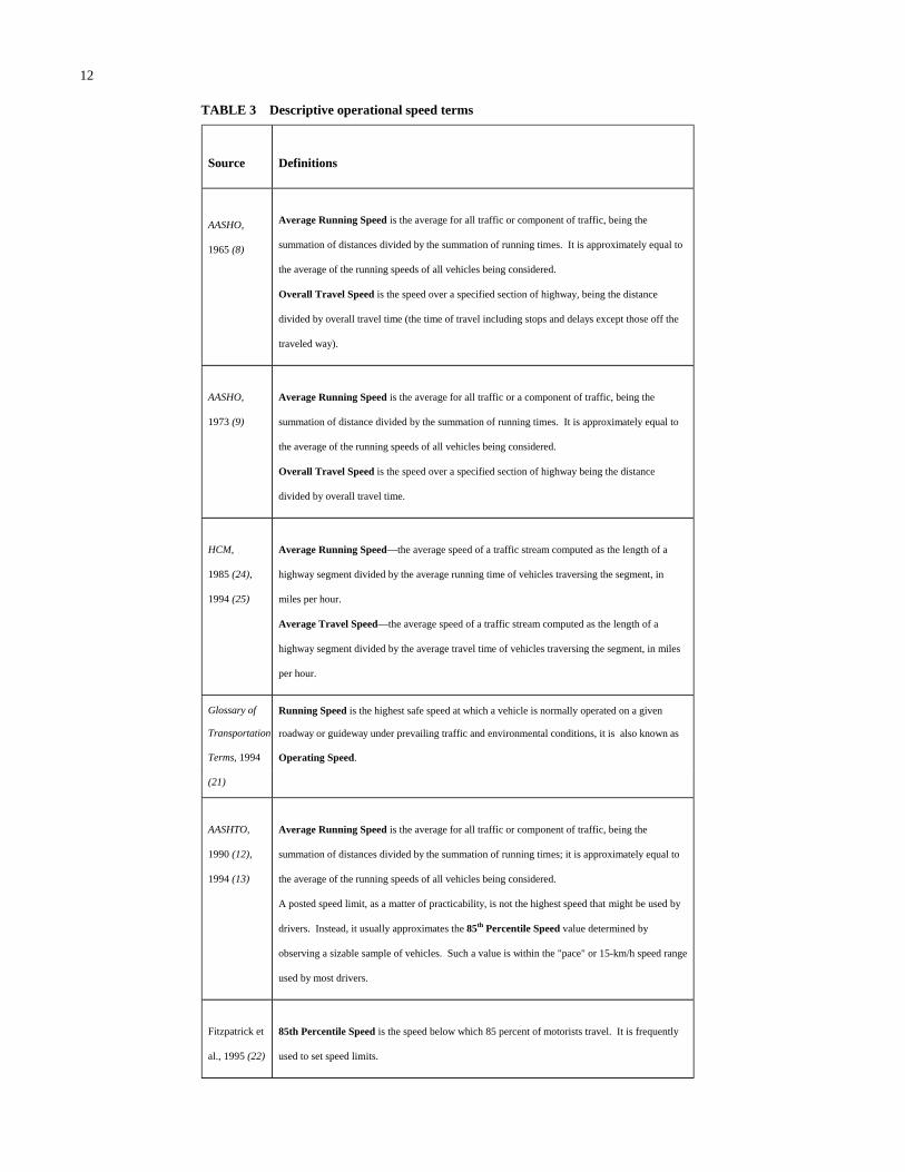
Today’s profession uses several additional speed terms,such as 85th percentile speed or pace speed. Table 3 listssuch speed terms and their respective definitions.

MAILOUT SURVEY

A mailout survey was conducted in early 1999 to developa better understanding of what definitions, policies, and val-ues are used by practicing engineers in the design of newroadways and improvements to existing roadways. Respon-dents were asked questions divided into four sections relat-ing to definitions, policies and practices, design values, andspeed values. Respondents were also asked to provide theircomments on the topic and information regarding their cur-rent position and previous experience.

The survey was mailed to the members of the AASHTOSubcommittee on Design. A total of 45 completed surveyswere received, representing 40 states. The respondents gen-erally were directors or managers within a design division ofa state department of transportation. The years of designexperience for the respondents ranged from 3 to 40, withmost having over 20 years of experience.

Appendix B contains more details on the findings from thesurvey. The findings from this survey were used to developimprovements or refinements to speed definitions that wereconsidered for inclusion in key reference documents such asthe Green Book and the MUTCD. Key findings include thefollowing:

• Most states use the 1994 Green Book definitions; how-ever, fewer respondents indicated that it was their pre-ferred definition.

• Design practices and policies vary from state to state.For example, in selecting the design speed of a new road,the functional class or the legal speed limit were mostcommonly used.

10

TABLE 2 Operating speed definitions

Source Definitions

HCM, 1950

(18)

The most significant index of traffic congestion during different traffic volumes, as far as drivers

are concerned, is the overall speed (exclusive of stops) which a motorist can maintain when

trying to travel at the highest safe speed. This overall speed is termed Operating Speed.

Matson et al.,

1955 (19)

Operating Speed is the highest overall speed, exclusive of stops, at which a driver can travel on

a given highway under prevailing conditions. It is the same as design speed when atmospheric

conditions, road-surface conditions, etc., are ideal and when traffic volumes are low.

HCM, 1965

(20)

Operating Speed is the highest overall speed at which a driver can travel on a given highway

under prevailing traffic conditions without at any time exceeding the safe speed as determined by

the design speed on a section-by-section basis.

AASHO,

1973 (9)


under favorable weather conditions and under prevailing traffic conditions without exceeding the

safe speed on a section-by-section basis used for design

Glossary of

Transportation

Terms, 1994

(21)

Running Speed is the highest safe speed at which a vehicle is normally operated on a given

roadway or guideway under prevailing traffic and environmental conditions, it is also known as

Operating Speed.

AASHTO,

1990 (12),

1994 (13)


under favorable weather conditions and under prevailing traffic conditions without at any time

exceeding the safe speed as determined by the design speed on a section-by-section basis.

Fitzpatrick et

al., 1995 (22)

Operating Speed is the speed at which drivers are observed operating their vehicles. The 85th

percentile of the distribution of observed speed is the most frequently used descriptive statistics

for the operating speed associated with a particular location or geometric feature.

TRB Special

Report 254,

1998 (23)

Operating Speed—Operating speed is the speed at which drivers of free-flowing vehicles

choose to drive on a section of roadway.

MUTCD,

1988 (14)

Operating Speed—A speed at which a typical vehicle or the overall traffic operates. May be

defined with speed values such as average, pace, or 85th percentile speeds.

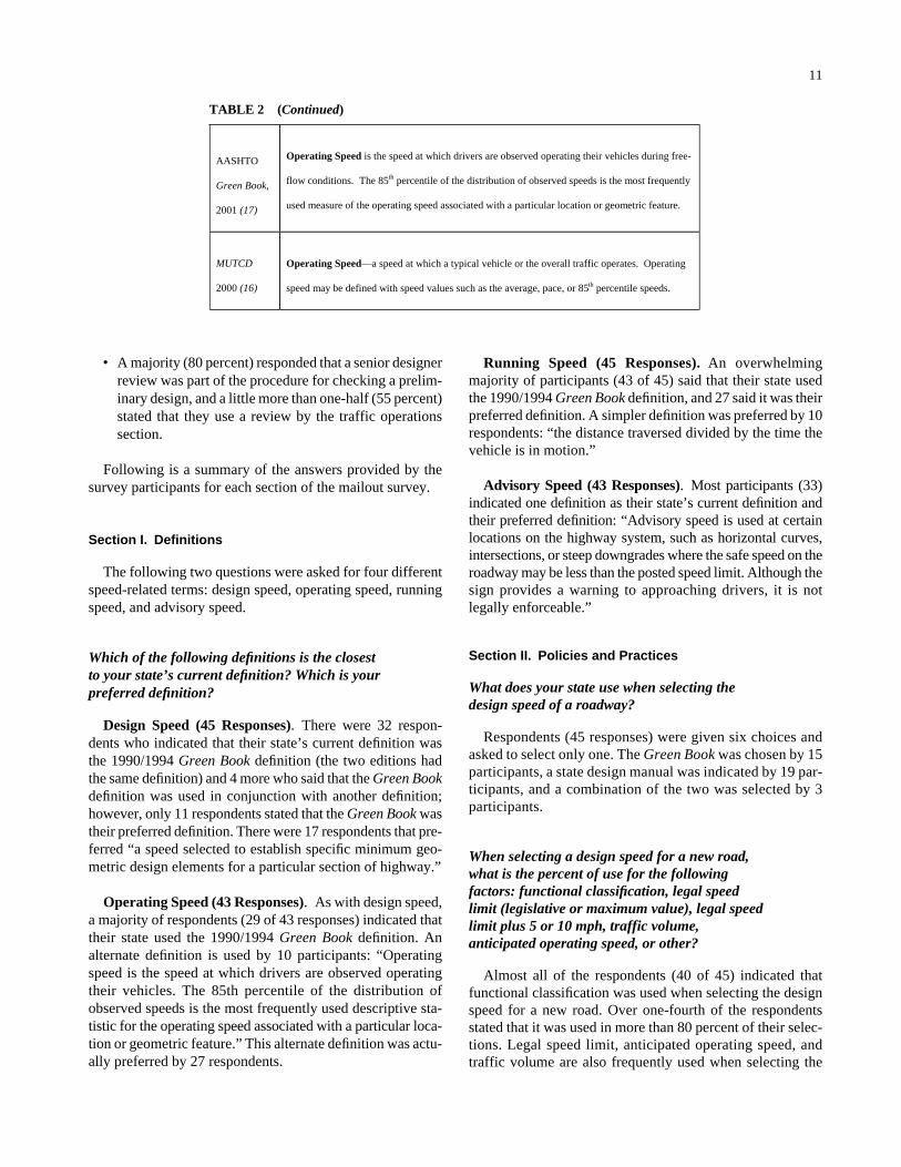
• A majority (80 percent) responded that a senior designerreview was part of the procedure for checking a prelim-inary design, and a little more than one-half (55 percent)stated that they use a review by the traffic operationssection.

Following is a summary of the answers provided by thesurvey participants for each section of the mailout survey.

Section I. Definitions

The following two questions were asked for four differentspeed-related terms: design speed, operating speed, runningspeed, and advisory speed.

Which of the following definitions is the closestto your state’s current definition? Which is yourpreferred definition?

Design Speed (45 Responses). There were 32 respon-dents who indicated that their state’s current definition wasthe 1990/1994 Green Book definition (the two editions hadthe same definition) and 4 more who said that the Green Bookdefinition was used in conjunction with another definition;however, only 11 respondents stated that the Green Book wastheir preferred definition. There were 17 respondents that pre-ferred “a speed selected to establish specific minimum geo-metric design elements for a particular section of highway.”

Operating Speed (43 Responses). As with design speed,a majority of respondents (29 of 43 responses) indicated thattheir state used the 1990/1994 Green Book definition. Analternate definition is used by 10 participants: “Operatingspeed is the speed at which drivers are observed operatingtheir vehicles. The 85th percentile of the distribution ofobserved speeds is the most frequently used descriptive sta-tistic for the operating speed associated with a particular loca-tion or geometric feature.” This alternate definition was actu-ally preferred by 27 respondents.

11

Running Speed (45 Responses). An overwhelmingmajority of participants (43 of 45) said that their state usedthe 1990/1994 Green Book definition, and 27 said it was theirpreferred definition. A simpler definition was preferred by 10respondents: “the distance traversed divided by the time thevehicle is in motion.”

Advisory Speed (43 Responses). Most participants (33)indicated one definition as their state’s current definition andtheir preferred definition: “Advisory speed is used at certainlocations on the highway system, such as horizontal curves,intersections, or steep downgrades where the safe speed on theroadway may be less than the posted speed limit. Although thesign provides a warning to approaching drivers, it is notlegally enforceable.”

Section II. Policies and Practices

What does your state use when selecting thedesign speed of a roadway?

Respondents (45 responses) were given six choices andasked to select only one. The Green Book was chosen by 15participants, a state design manual was indicated by 19 par-ticipants, and a combination of the two was selected by 3participants.

When selecting a design speed for a new road,what is the percent of use for the followingfactors: functional classification, legal speedlimit (legislative or maximum value), legal speedlimit plus 5 or 10 mph, traffic volume,anticipated operating speed, or other?

Almost all of the respondents (40 of 45) indicated thatfunctional classification was used when selecting the designspeed for a new road. Over one-fourth of the respondentsstated that it was used in more than 80 percent of their selec-tions. Legal speed limit, anticipated operating speed, andtraffic volume are also frequently used when selecting the

TABLE 2 (Continued)

AASHTO

Green Book,

2001 (17)

Operating Speed is the speed at which drivers are observed operating their vehicles during free-

flow conditions. The 85th percentile of the distribution of observed speeds is the most frequently

used measure of the operating speed associated with a particular location or geometric feature.

MUTCD

2000 (16)

Operating Speed—a speed at which a typical vehicle or the overall traffic operates. Operating

speed may be defined with speed values such as the average, pace, or 85th percentile speeds.

12

TABLE 3 Descriptive operational speed terms

Source

Definitions

AASHO,

1965 (8)

Average Running Speed is the average for all traffic or component of traffic, being the

summation of distances divided by the summation of running times. It is approximately equal to

the average of the running speeds of all vehicles being considered.

Overall Travel Speed is the speed over a specified section of highway, being the distance

divided by overall travel time (the time of travel including stops and delays except those off the

traveled way).

AASHO,

1973 (9)

Average Running Speed is the average for all traffic or a component of traffic, being the

summation of distance divided by the summation of running times. It is approximately equal to


Overall Travel Speed is the speed over a specified section of highway being the distance

divided by overall travel time.

HCM,

1985 (24),

1994 (25)

Average Running Speed—the average speed of a traffic stream computed as the length of a

highway segment divided by the average running time of vehicles traversing the segment, in

miles per hour.

Average Travel Speed—the average speed of a traffic stream computed as the length of a

highway segment divided by the average travel time of vehicles traversing the segment, in miles

per hour.

Glossary of

Transportation

Terms, 1994

Running Speed is the highest safe speed at which a vehicle is normally operated on a given

roadway or guideway under prevailing traffic and environmental conditions, it is also known as

(21)

Operating Speed.

AASHTO,

1990 (12),

1994 (13)

Average Running Speed is the average for all traffic or component of traffic, being the

summation of distances divided by the summation of running times; it is approximately equal to


A posted speed limit, as a matter of practicability, is not the highest speed that might be used by

drivers. Instead, it usually approximates the 85th Percentile Speed value determined by

observing a sizable sample of vehicles. Such a value is within the "pace" or 15-km/h speed range

used by most drivers.

Fitzpatrick et

al., 1995 (22)

85th Percentile Speed is the speed below which 85 percent of motorists travel. It is frequently

used to set speed limits.

13

TABLE 3 (Continued)

HCM, 1997

(26)

Average Running Speed—This is also called "space mean speed" in the literature. It is a traffic

stream measurement based on the observation of vehicle travel times traversing a section of

highway of known length. It is defined as the length of the segment divided by the average

running time of vehicles to traverse the segment. "Running time" includes only time that vehicles

spend in motion.

Average Travel Speed—This is also a traffic stream measure based on travel time observations

over a known length of highway. It is defined as the length of the segment divided by the

average travel time of vehicles traversing the segment, including all stopped delay times. It is

also a "space mean speed," because the use of average travel times effectively weights the

average according to length of time a vehicle occupies the defined roadway segment or "space."

TRB

SpecialReport254 (23)

10-mph Pace Χ—The 10-mph pace is the 10-mph range encompassing the greatest percentage of

all the measured speeds in a spot speed study. It is described by the speed value at the lower end

of the range and the percentage of all vehicles that are within the range; as such, it is an

alternative indicator of speed dispersion. Most engineers believe that safety is enhanced when

the 10-mph pace includes a large percentage (more than 70 percent) of all the free-flowing

vehicles at a location. (Note: 10 mph = 16.1 km/h).

85th Percentile Speed — The 85th percentile speed is the speed at or below which 85 percent of

the free-flowing vehicles travel. Traffic engineers have assumed that this high percentage of

drivers will select a safe speed on the basis of the conditions at the site. The 85th percentile

speed has traditionally been considered in an engineering study to establish a speed limit. In

most cases, the difference between the 85th percentile speed and the average speed provides a

good approximation of the speed sample’s standard deviation.

Advisory Speed — At certain locations on the highway system, such as horizontal curves,

intersections, or steep downgrades, the sage speed on the roadway may be less than the posted

speed limit. Rather than lowering the regulatory speed limits at each of these locations, traffic

engineers often place standard warning signs accompanied by a square black-and-yellow

advisory speed plate. Although this sign provides a warning to approaching drivers, it is not

legally enforceable.

Average Speed — The average (or mean) speed is the most common measure of central

tendency. Using data from a spot speed study, the average is calculated by summing all the

measured speeds and dividing by the sample size, n.


design speed of a new road. Almost one-half of those indicat-ing legal speed limit used that factor in 50 percent of theirselections, while the other half used the factor in 10 to 30 per-cent of their selections. Volume and anticipated operatingspeed were used less frequently in the selection of a new road’sdesign speed. There were 13 responses given for the “other”factor, 8 of which mentioned terrain and/or topography; 9 ofthe 13 answers for these factors ranged from 20 to 40 percent.

After indicating the factors used in design, respondentswere asked to explain the processes they used; their answersfocused on the consideration of state law, area land use, func-tional classification, and state design manuals.

When selecting a design speed for a project withfew changes (i.e., when alignment or crosssection is changed for some of the elements),what is the percent of use for the followingfactors: existing design speed, design speed thatwould have been selected for a new road, existingposted speed limit, anticipated operating speed,existing operating speed, speed associated withthe functional classification of the road, or other?

Responses to this question were highly mixed. Over one-half of the respondents (24 of 45) indicated that existing design

14

speed, existing posted speed limit, and anticipated operatingspeed were used when selecting the new design speed. Twentyof the answers for existing design speed ranged from 10 to 50percent usage. The distribution of answers for existing postedspeed limit and anticipated operating speed were identical,with nine responses between 10 and 30 percent, nine responsesbetween 40 and 60 percent, and six responses of 70 percentor greater. There were 17 responses indicating the use of thedesign speed that would have been selected for a new road,with 12 between 10 and 60 percent. There were also 17responses for the speed associated with the functional classifi-cation of the road, with 15 between 10 and 60 percent. Therewere 12 responses given in favor of existing operating speed,ranging from 10 to 50 percent, and there were 12 responsesthat indicated other factors. There was no predominant “other”factor, but some of the factors mentioned included runningspeed, terrain, accident history, traffic volume, and GreenBook guidelines. The respondents typically gave between 10and 60 percent as the percent of use for those factors, althoughthree were between 90 and 100 percent.

When selecting a design speed for a project wherethe roadway is changing in its functional class(e.g., when a two-lane highway is expanded to

TABLE 3 (Continued)

MUTCD,

1998 (14)

85th Percentile Speed — The speed at or below which 85 percent of the motorized vehicles

travel.

Average Speed—The summation of the instantaneous or spot-measured speeds at a specific

location of vehicles divided by the number of vehicles observed.

Pace Speed—The highest speed within a specific range of speeds which represents more

vehicles than in any other like range of speed. The ranges of speeds typically used is 10 mph.

MUTCD,

2000 (16)

85th Percentile Speed—The speed at or below which 85 percent of the motorized vehicles

travel.

MUTCD,

2000 (16)


location of vehicles divided by the number of vehicle observed.

Pace Speed—The highest speed within a specific range of speeds that represents more vehicles

than in any other like range of speed. The range of speeds typically used is 10 km/h or 10 mph.

MUTCD,

2000 (16)


location of vehicles divided by the number of vehicles observed.

Pace Speed—The highest speed within a specific range of speeds that represents more vehicles

than in any other like range of speed. The range of speeds typically used is 10 km/h or 10 mph.

add capacity and becomes a suburban arterial),what is the percent of use for the followingfactors: existing design speed, design speed thatwould have been selected for a new road, existingposted speed limit, anticipated operating speed,existing operating speed, speed associated withthe functional classification of the road, or other?

Two-thirds of the respondents (30 of 45) indicated thatthey used the design speed that would have been selected fora new road. Eighteen of those respondents stated that it wasused in between 20 and 60 percent of their selections, whileeight indicated it was used in more than 90 percent. Speedassociated with the functional classification of the road waschosen by 24 respondents; 21 answers were between 10 and80 percent, while the remaining answers were between 90and 100 percent. Existing posted speed limit, existing designspeed, anticipated operating speed, and existing operatingspeed are also frequently used when selecting the design speedof a new road. Of the 45 responses for these four factors, allbut five were between 10 and 60 percent. There were 10responses given for other factors, which mentioned “all of theabove,” terrain, traffic volume, and accident history; answersfor these factors ranged between 10 and 100 percent.

Once a preliminary design has been completed,what is the procedure for checking the design(check all that apply)?

A large number of respondents (39 of 45) said that they usea senior designer review, and more than one-half (27) used atraffic operations section review. Some (13) also used a safetysection review and nearly half (22) used some other methodsfor checking the design. These other methods included reviewby the state design office or district personnel (9), review byother sections such as construction and maintenance (6), andpeer review or quality assurance team review (6).

When justification is needed for a designexception (i.e., when all the elements for aroadway do not meet the selected design speed),what is the percent of use for the followingfactors: incremental cost, environmental, right ofway, consistency with adjacent section, safety,historical preservation/societal concerns, publicdemands/expectations, or other?

Respondents (45 responses) indicated that they all use awide variety of factors; all of the factors listed received at least28 responses, and the vast majority of responses describedusage of less than 30 percent for each factor. Factors listedincluded incremental cost, environmental, right of way, con-sistency with adjacent section, safety, historical preservation/societal concerns, and public demands/expectations.

15

When reconstructing a roadway, have you had asituation where the design speed of an existingroadway is greater than or equal to the operatingspeed and the citizens would like lower operatingspeeds on the facility?

Responses (45 responses) to this question were dividedfairly evenly, with 25 answering “yes” and 20 answering“no.” For those who answered “yes,” 10 respondents indi-cated that conditions are reviewed on a case by case basis,perhaps with a speed study, and are sometimes lowered. Fiveresponses indicated that nothing was done or that citizenswere informed as to how speed limits are set and no changeswould be made. Three responses referred to traffic calming,and three responses indicated that speed limit changes wereunder the authority of a specific entity, either local, regional,or statewide. The remaining responses generally referred toreconstruction or trial speed limits.

Effects of Geometric Elements on Speed

All of the respondents indicated that narrow lane widthscause drivers to drive slower on freeways, and most (89 per-cent) believe that narrow lane widths cause drivers to driveslower on local streets. When wide lane widths exist, most ofthe respondents believe they do not affect drivers’ speeds onfreeways but do affect local street speeds.

There were 29 respondents (71 percent) who indicated thatshoulder width does affect speed. About two-thirds believednarrow shoulders cause drivers to drive slower on both urbanand rural freeways. About one-half of the respondents believethat wide paved shoulders cause drivers to drive faster.

A large majority (more than 80 percent) believe that nar-row clear zone/lateral clearance widths affect the speed thatdrivers select on both urban and rural roads. A smaller major-ity (about 60 percent) believe that wide lateral clearance/clear zone widths cause drivers to drive faster.

More than 60 percent of those responding believe thatraised medians and two-way left-turn lanes (TWLTLs) affectthe speed that drivers select.

Section III. Speed Values

An initial step in the design process is defining the functionthat a facility is to serve. The ability of the roadway to providethat function is related to the anticipated volume of traffic, theanticipated operating speed, and the geometric criteria present.For the following classes of roadways (shown as columns inTable 4), please use your engineering judgment to provide theappropriate speed (mph) for each item (shown as rows).

Table 4 lists the most common responses given for each cat-egory. Appendix B includes additional details on the findings.

Section IV. Design Values

An initial step in the design process is defining the functionthat a facility is to serve. The ability of the roadway to pro-vide that function is related to the anticipated volume of traf-fic, the anticipated operating speed, and the geometric criteriapresent. For the following classes of roadways (shown ascolumns in Table 5), please use your engineering judgmentto provide the value or range of appropriate values for eachitem (shown as rows).

Table 5 lists the most common responses given for each cat-egory. Appendix B includes additional details on the findings.

16

Section V. General Comments/Concerns

Respondents were asked to provide any comments or con-cerns they had on this topic. The most common concerns men-tioned the inconsistencies between design speed, posted speed,and operating speed. Respondents noted that there was a lackof a clear relationship between the three, and often the operat-ing speed is higher than the design speed and/or posted speed.This issue was reported to lead to the possibility of increasedliability for the engineer or the agency. Related comments indi-cated that standards for design speed should allow flexibilityfor topographic features and local/regional driving attitudes.

TABLE 4 Speed values from mailout survey

URBAN

Two lanes

Multilane Arterial

Terrain

Speed Terms

Local

Collector

Undivided

Divided

Freeway

Anticipated Operating

Speed (mph)

30

35-45

45-55

50-60

60-70

Anticipated Posted

Speed (mph)

30

30-45

45

45-55

55

Level /

Rolling

Design

Speed (mph)

30

35-50

45-50

45-60

60-70


Speed (mph)

25-35

30-45

40-50

50

55-65

Anticipated Posted

Speed (mph)

25-30

35-40

45

45

55-60

Mountain

Design

Speed (mph)

30

40

40-50

50

60-65

DESIGN ELEMENT REVIEW

A goal of this research was to evaluate current procedures,especially how speed is used as a control in existing policyand guidelines. A detailed evaluation was conducted to deter-mine how speed relates to design elements. The review deter-mined (1) whether design speed is used to select the designelement value, (2) whether there is a relationship between adesign element and the operating speed, and (3) whether thereis a relationship between a design element and the safety on aroadway.

17

For this review, the researchers established three levels atwhich design speed can affect a design element (or a designelement component).

• Design speed can be directly related to the design elementor component in that the design speed is used to select theappropriate element or component. This direct relationshipassumes and consequently designs for an effect of speed.

• Design speed can be indirectly related to an element orcomponent. Under this scenario, design speed is not usedto select the design element or component, but operating

TABLE 4 (Continued)

RURAL

Two lanes

Multilane Highways

Terrain

Speed Terms

Low

High

Undivided

Divided

Freeway


Speed (mph)

35-55

60-65

60-65

60-70

70-75

Anticipated Posted

Speed (mph)

55

55

55

65

70

Level /

Rolling

Design

Speed (mph)

60

60

60

60-70

70


Speed (mph)

30-35

30-60

50-60

50-60

60-70

Anticipated Posted

Speed (mph)

25-35

55

45-55

50-60

55-65

Mountain

Design

Speed (mph)

30-40

35-60

50-60

50-60

65-70

speed is. Operating speed, as defined in the AASHTOGreen Book (13), is termed average running speed. Anindirect relationship between design speed and designelements or components is defined herein as when anoperating speed is used to select the appropriate designelement or component and when the operating speed isbased on some assumed relationship to design speed.

18

(Note: the assumed design speed/operating speed rela-tionship used for the selection of certain elements/components, however, is not well defined, as demon-strated in the subsequent sections.)

• Design speed may not be directly related to an elementor component. Here, the element under consideration isdetermined from some other method than design speed.

TABLE 5 Design values from mailout survey

Maximum Grade (%) 15 8-12 5-11 5-11 3-6

URBAN

Two lanes

Multilane Arterial

Item

Local

Collector

Undivided

Divided

Freeway

ROADWAY CROSS-SECTION ELEMENTS

Lane Width (ft)

10-12

10-12

11-12

11-12

12

Shoulder Width (ft)

2-8

0-11

10-12

10

10-12

Clear Zone (ft)

1.5 (curb)

5-20 (no curb)

1.5 (curb)

10-30 (no curb)

1.5 (curb)

12-30 (no curb)

10-44

30

Median Width (ft)

< 30

> 30

ROADWAY ALIGNMENT ELEMENTS

Radius (minimum) (ft)

300-400

200-1000

200-1000

262-2475

50-3000

Superelevation (ft/ft)

0.04

0.04

0.04

0.06

0.06

19

TABLE 5 (Continued)

RURAL

2 lanes

Multilane Highways

Item

Low

High

Undivided

Divided

Freeway

ROADWAY CROSS-SECTION ELEMENTS

Lane Width (ft)

10-12

10-12

10-12

11-12

12

Shoulder Width (ft)

2-8

8-10

8-10

10-12

10-12

Clear Zone (ft)

10

30

30

30

30

Median Width (ft)

40-60

45-90

ROADWAY ALIGNMENT ELEMENTS

Radius (minimum) (ft)

<1000

252-2477

1000-2000

1000-2000

1500-2000


0.06-0.08

0.06-0.08

0.08

0.08

0.08

Maximum Grade (%)

0.5-16

0.5-16

4-6

4-6

3-6

Most of the design elements or their values are eitherdirectly or indirectly selected based on design speed. In a fewsituations the type of roadway is used to determine the designelement. These relationships were identified from the GreenBook and are summarized in Table 6.

Several of the design elements have been found to have adefinable relationship with operating speed (see Table 7). Fora design element component to be directly related to operat-ing speed, the operational studies reviewed herein must showevidence that indeed the component under study affects oper-ating speed. When the findings of the operational studiesresult in a mixed review, the relationship is classified asinconclusive. If no relationship has been determined and thedesign element component in question has been adequatelystudied, then the design component is classified as having norelationship with operating speed. In some cases the rela-tionship is strong, such as for horizontal curves, and in othercases the relationship is weak, such as for lane width. In allcases when a relationship between the design element andoperation speed exist, there are ranges when the influence ofthe design element on speed is minimal. For example, a gradeof 6 or 7 percent influences the operating speed of trucks andsome passenger vehicles, while grades of 1 or 2 percent donot influence operating speeds.

A third review investigated the safety implications of designelements. While the relationship between a design element andoperating speed may be weak, the consequences of selecting aparticular value may have safety implications. An example isthe width of shoulders. Research has shown that no distinc-tive relationship exists between shoulder width and operat-ing speed (note that the clear zone component was reviewedseparately). Using such a finding to encourage the use of noshoulders or minimal width shoulders on high-speed facili-ties could have negative safety implications. Table 8 sum-marizes the findings from the safety review.

The reviews demonstrated that there are known relation-ships between safety and design features and that the selec-tion of design features varies based on the operating speed.Therefore, design elements (investigated within this study)should be selected with some consideration of the anticipatedoperating speed of the facility. In some cases the considera-tion should take the form of selecting a design element valuewithin a range that has minimal influence on operating speedor that would not adversely affect safety. In other cases theselection of a design element value should be directly relatedto the anticipated operating speed.

PREVIOUS RELATIONSHIPS

Several studies have investigated the relationships betweenthe various speed elements. Some of the studies have tried topredict operating speed using roadway characteristics, whileothers have attempted to identify the relationship betweenposted speed limit and operating speed. Tables 9 and 10 sum-marize the roadway and roadside variables found to influence

20

operating speed. Appendix D contains summaries of the rela-tionships identified in the literature by functional classifica-tion. Following are key findings on the relationship betweendesign elements and operating speed.

Two-Lane Rural Highways

• A 2000 FHWA study (36) collected speed data at morethan 200 two-lane rural highway sites. The study devel-oped speed prediction equations for several conditions,such as vertical curves on horizontal tangents, horizon-tal curves on grade, etc. The variables that influencedoperating speed included radius, grade, and K-value (rateof vertical curvature). For those situations where a sta-tistical relationship could not be established, a review ofthe data and engineering judgment were used to set arounded maximum operating speed value of 62.1 mph(100 km/h).

• The analyses of 162 tangent sections on two-lane ruralhighways (42) showed that when determining 85th per-centile speeds in the middle of a tangent section, it is nec-essary to observe a longer section—one that includes thepreceding and succeeding curves—since these consti-tute the primary variables affecting speed. The influenceof other, secondary geometric variables was investigatedand was found to not impact speed as much as the pri-mary variables.

• A 1991 article (43) found that for 28 horizontal curves,all of the curves with a design speed of 50 mph (80.5km/h) or less had 85th percentile speeds that exceededthe design speed. Only on the single 60-mph (96.6-km/h)design speed curve was the observed 85th percentilespeed less than the design speed.

• In a 1994 FHWA study, speed data were collected at 138horizontal curves on 29 rural two-lane highways in fivestates (33). The data in these studies clearly showed thatthe radius of the horizontal curve affects operating speed.

• The NCHRP study on stopping sight distance measuredoperating speed on limited sight distance crest verticalcurves (15). The data showed that as the inferred designspeed increases (i.e., greater available sight distance),operating speeds are higher. The mean reductions inspeed between the control and crest sections tend toincrease as available sight distance is decreased; how-ever, the reduction in speed is less than that suggestedby the then-current AASHTO criteria.

• McLean (30, 44) found design speed/operating speed dis-parities on rural two-lane highways in Australia. Hori-zontal curves with design speeds less than 55.9 mph (90km/h) had 85th percentile speeds that were consistentlyfaster than the design speed, whereas curves with designspeeds greater than 55.9 mph (90 km/h) had 85th per-centile speeds that were consistently slower than thedesign speed.

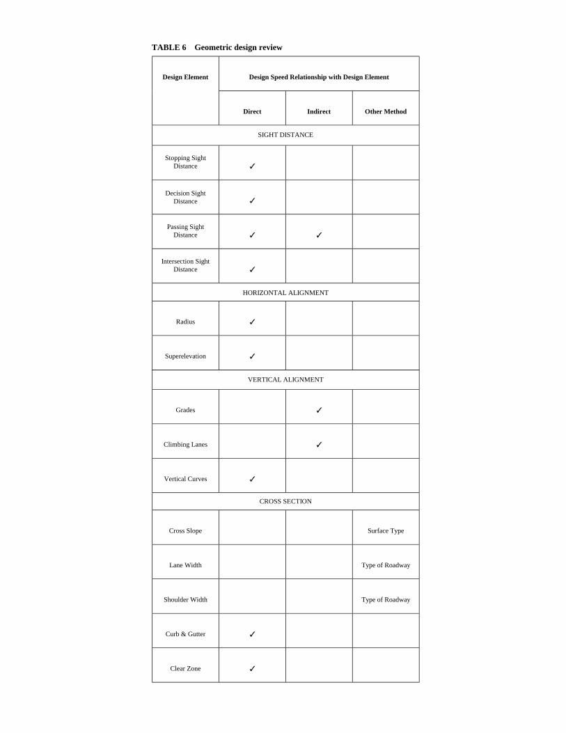
TABLE 6 Geometric design review

Design Speed Relationship with Design Element

Design Element

Direct

Indirect

Other Method

SIGHT DISTANCE

Stopping Sight Distance

✓

Decision Sight Distance

✓

Passing Sight Distance

✓

✓

Intersection Sight Distance

✓

HORIZONTAL ALIGNMENT

Radius

✓

Superelevation

✓

VERTICAL ALIGNMENT

Grades

✓

Climbing Lanes

✓

Vertical Curves

✓

CROSS SECTION

Cross Slope

Surface Type

Lane Width

Type of Roadway

Shoulder Width

Type of Roadway

Curb & Gutter

✓

Clear Zone

✓

22

TABLE 7 Operating speed review

Operating Speed Relationship with Design Element

Design Element

Direct

Inconclusive

No

SIGHT DISTANCE


yes (with limits)


✓


✓


✓


Radius

✓

Superelevation

✓

VERTICAL ALIGNMENT

Grades

✓

Climbing Lanes ✓

Vertical Curves

✓

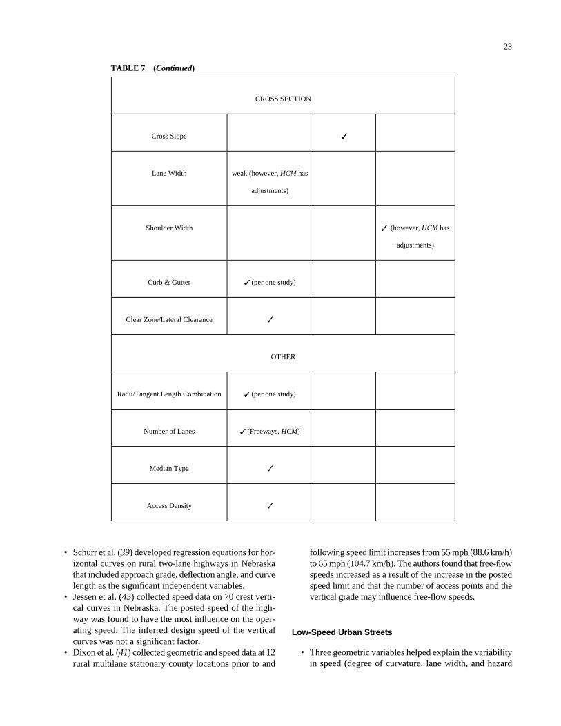
• Schurr et al. (39) developed regression equations for hor-izontal curves on rural two-lane highways in Nebraskathat included approach grade, deflection angle, and curvelength as the significant independent variables.

• Jessen et al. (45) collected speed data on 70 crest verti-cal curves in Nebraska. The posted speed of the high-way was found to have the most influence on the oper-ating speed. The inferred design speed of the verticalcurves was not a significant factor.

• Dixon et al. (41) collected geometric and speed data at 12rural multilane stationary county locations prior to and

23

following speed limit increases from 55 mph (88.6 km/h)to 65 mph (104.7 km/h). The authors found that free-flowspeeds increased as a result of the increase in the postedspeed limit and that the number of access points and thevertical grade may influence free-flow speeds.

Low-Speed Urban Streets

• Three geometric variables helped explain the variabilityin speed (degree of curvature, lane width, and hazard

TABLE 7 (Continued)

CROSS SECTION

Cross Slope

✓

Lane Width

weak (however, HCM has

adjustments)

Shoulder Width

✓ (however, HCM has

adjustments)

Curb & Gutter

✓ (per one study)

Clear Zone/Lateral Clearance

✓

OTHER

Radii/Tangent Length Combination

✓ (per one study)

Number of Lanes

✓ (Freeways, HCM)

Median Type

✓

Access Density ✓

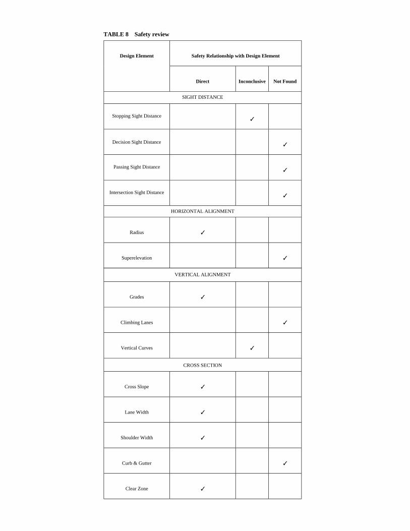
TABLE 8 Safety review

Safety Relationship with Design Element

Design Element

Direct

Inconclusive

Not Found

SIGHT DISTANCE


✓


✓


✓


✓


Radius

✓

Superelevation

✓

VERTICAL ALIGNMENT

Grades

✓

Climbing Lanes

✓

Vertical Curves

✓

CROSS SECTION

Cross Slope

✓

Lane Width

✓

Shoulder Width

✓

Curb & Gutter

✓

Clear Zone

✓

25

TABLE 9 Variables influencing midpoint horizontal curve operating speed

Influencing Roadway or Roadside Variable

Author (year)

Functional Class

Deg

ree

of C

urve

Rad

ius

Len

gth

ofC

urve

Def

lect

ion

Ang

le

Infe

rred

Spe

ed

Lan

e W

idth

Haz

ard

Rat

ing

Acc

ess

Den

sity

Spe

ed L

imit

Roa

dsid

e

Gra

de

Med

ian

Pre

senc

e

Seve

ral V

aria

bles

*

R2

Tarigan (1954) (27)

X

74

Dept of Main Roads, New

South Wales (1969) (28)

X

83

Emmerson (1969) (29)

X

na

McLean (1979) (30)

X

X

92

Glennon (1983) (31)

X

84

Lamm (1988) (32)

Rural Two-Lane

X

79

Krammes et al. (1993)

(33)

Rural Two-Lane

X

X

X

82

Islam et al. (1994) (34)

X

98

Fitzpatrick et al. (1995)

(22)

Suburban Arterials

X

72

Poe et al. (1996) (35)

Low-Speed Urban

X

X

X

X

X

X

X

X

X

75


rating) on horizontal curves on a low-speed urban streetenvironment (defined as below 40 mph [64.4 km/h]) ina 2000 study (37).

• An Arkansas study examined the relationship amongurban street function (i.e., arterial versus local traffic),width, and resulting speed (46). For the streets having

26

more local street characteristics (such as shorter length),the data did show a statistically significant differencebetween the mean speeds on wider and narrower streetsegments. When adjusted by eliminating vehicles thatturned onto or off of the street in midsegment, themagnitudes of the differences were less than 4.3 mph

TABLE 9 (Continued)


(36)

Rural Two-Lane

X X 53-

76

Poe and Mason (2000)

(37)

Low Speed Urban

X

X

X

na


(38)

Suburban Arterial

X

X

X

75


(38)

Suburban arterial

(w/o speed limit)

X

X

62

Schurr et al. (2002) (39)

Rural Two-Lane

X

X

X

46

*Several Variables = sight distance, curbs, road surface, superelevation, land use, centerline markings, warning

signs.


Author (year)

Functional Class

Deg

ree

of C

urve

Rad

ius

Len

gth

ofC

urve

Def

lect

ion

Ang

le

Infe

rred

Spe

ed

Lan

e W

idth

Haz

ard

Rat

ing

Acc

ess

Den

sity

Spe

ed L

imit

Roa

dsid

e

Gra

de

Med

ian

Pre

senc

e

Seve

ral V

aria

bles

*

R2

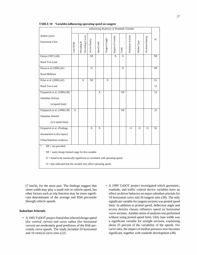
(7 km/h), for the most part. The findings suggest thatstreet width may play a small role in vehicle speed, butother factors such as trip function may be more signifi-cant determinants of the average and 85th percentilethrough vehicle speeds.

Suburban Arterials

• A 1995 TxDOT project found that inferred design speed(for vertical curves) and curve radius (for horizontalcurves) are moderately good predictors of the 85th per-centile curve speeds. The study included 10 horizontaland 10 vertical curve sites (22).

27

• A 1999 TxDOT project investigated which geometric,roadside, and traffic control device variables have aneffect on driver behavior on major suburban arterials for19 horizontal curve and 36 tangent sites (38). The onlysignificant variable for tangent sections was posted speedlimit. In addition to posted speed, deflection angle andaccess density classes influence speed on horizontalcurve sections. Another series of analyses was performedwithout using posted speed limit. Only lane width wasa significant variable for straight sections, explainingabout 25 percent of the variability of the speeds. Forcurve sites, the impact of median presence now becomessignificant, together with roadside development (38).

TABLE 10 Variables influencing operating speed on tangent


Author (year)

Functional Class

Lan

e W

idth

Prec

edin

g &

Succ

eedi

ng C

urve

s

Acc

ess

Den

sity

Spe

ed L

imit

Tan

gent

Len

gth

Reg

ion

of C

ount

ry

Gra

de

Ped

estr

ian

Act

ivit

y

Med

ian

Typ

e

On-

Stre

et P

arki

ng

R2

Parma (1997) (40)

Rural Two-Lane

NF X X NP

Dixon et al (1999) (41)

Rural Multlane

O O NP

Polus et al. (2000) (42)

Rural Two-Lane

X NF X 23-

55

Fitzpatrick et al. (1999) (38)

Suburban Arterial

(w/speed limit)

X NF 53

Fitzpatrick et al. (1999) (38)

Suburban Arterial

(w/o speed limit)

X NF 25

Fitzpatrick et al. (Findings

documented in this report)

Urban/Suburban roadways

X X O O O 92

* NP = not provided.

NF = study design limited range for this variable.

X = found to be statistically significant or correlated with operating speed.

O = data indicated that the variable may affect operating speed.

Freeways

• A case study was conducted on the effects of visibilityand other environmental factors on driver speed on a100-mi (161-km) stretch of Interstate 84 in southeastIdaho and northwest Utah (47). The data presentedshow that the drivers at the site respond to poor envi-ronmental conditions by reducing their speeds. The meanspeed reduction for all vehicles was 5.0 mph (8 km/h)during the two fog events and 11.9 mph (19 km/h) duringthe 11 snow events.

Urban Roadways

• In a 1962 study on operating speeds within the urbanenvironment, Rowan and Keese concluded that sub-stantial speed reductions occurred when sight distancewas less than 1,000 to 1,200 ft (305 to 366 m) and thatthe introduction of a curbed urban cross section and theadjacent land use (residential or commercial develop-ment) had an influence on speed reduction (48). Lateralrestrictions (trees and shrubbery) were found to be agreater influence on speed reduction than developmentdensity.

Multiple Roadway Types

• In 1966, Oppenlander reviewed the literature to identifyvariables influencing spot speed (49). The roadway char-acteristics determined to be most significant includedfunctional classification, curvature, gradient, length ofgrade, number of lanes, and surface type. Sight distance,lateral clearance, and frequency of intersections werealso determined to have an influence.

• In 1989, Garber and Gadiraju examined speed varianceson 36 roadway locations including interstates, arterials,and rural collectors (50). Analysis of variance tests founddesign speed and highway types significant, while timeand traffic volumes were not significant (50).

FIELD STUDIES

The driver’s view of a road can provide information onappropriate performance. For example, a view of a freewaywith its ramps and concrete median barrier indicates that highoperating speeds are expected. A freeway’s purpose is clearlydefined as mobility, and it tends to have high operatingspeeds in the range of 55 mph (88.5 km/h) and greater (withthe obvious exception of congested conditions). At the otherend of the spectrum is the local street, which has the purposeof providing access. Characteristics of local streets includeon-street parking, residential driveways, and other featuresthat indicate that lower operating speeds are appropriate.These facilities generally operate at speeds less than 30 or 35

28

mph (48.3 or 56.3 km/h). Between these extremes are col-lectors and arterials, which provide a mix of access and mobil-ity. Along with the mix of access and mobility comes a mixof operating speeds. The profession is seeking to better under-stand what features influence speeds on a roadway. If thosefeatures could be identified, then roadways could be designedto better influence the performance of drivers.

Site Selection

The general criteria used to select study sites are summa-rized in Table 11. These criteria were selected to provide adegree of uniformity and minimize the effects of elementsnot under consideration in this study. They were developedbased on the research team’s knowledge, especially on expe-riences from collecting similar data in previous projects. Inaddition to the criteria listed in Table 11, a goal was to selectsites from different regions of the United States. Data werecollected in seven cities located in six states:

• Little Rock, Arkansas,• St. Louis, Missouri,• Nashville, Tennessee,• Portland, Oregon,• Boston, Massachusetts, and• College Station and Houston, Texas.

To focus the site selection process, key variables wereselected for emphasis in this effort. Based on the findingsfrom previous studies (36, 38), the variables selected includedfunctional classification (arterial, collector, and local), edgetreatment (i.e., curb and gutter versus shoulder), and speedlimit. The data collected as part of the NCHRP 15-18 projectemphasized suburban/urban data because of the amount ofrural data available from previous FHWA projects (33, 36).

TABLE 11 Site selection criteria

Control

Criteria

Grade

Terrain

Surface Condition

Sight Distance

Headway/Tailway

Distance from Adjacent Horizontal Curve

Distance from Adjacent Signal or STOP Sign

+4% to -4%

Level to Rolling

Fair to Good

Adequate

5/3 s

0.1 mi

0.2 mi

Data Collection

The data collection effort included obtaining both the char-acteristics of the site and the speed data of vehicles at the site.

Site Characteristics

The site characteristic data collected at each study site arelisted in Table 12. Data focused on characteristics of the areabetween the upstream and downstream controls of the studysite except signal density, which used the number of signalswithin a mile of either side of the site. Each cross-section fea-ture was measured and recorded in the field. The presence ofthe following features was recorded: bike lane, on-streetparking, and type of median. Also, the number of lanes andthe type of edge treatment (shoulder, curb and gutter, etc.)

29

were noted. A measuring wheel was used to obtain the widthof each lane, median, and bike lane, if present.

Recording the characteristics of the roadside features for asite was more involved than collecting the data for the othersite variables. Measurements were made for some of the fea-tures and then were converted into a rating scale in the office.Determination of pedestrian and roadside characteristics wasbased on measurements and observations made at the studysites and observations from pictures and video taken at thesites. Roadside development was recorded as being residential,commercial/industrial, park/school/campus, farm, and trees/cliff/mountain. The residential and commercial/industrialcategories were expanded in the office during data analysisusing the video and pictures of the sites. The residential clas-sification was split into single-family residential and multi-family residential. Commercial/industrial was split into oneof four subcategories: multistory office buildings, low-story

TABLE 12 Site characteristics data collected at each study site

Site

• Area type (urban, suburban, rural)

• Functional class (arterial, collector, local)

• Date/time

• City

• Collector’s name

• Street

• Weather

Cross Section

• Number of lanes

• Lane width (per lane)

• Total pavement width

• Shoulder (none, curb & gutter, flush)

• Parking

• Bike lane

• Median type and width

Roadside

• Roadside development (per direction)

• Access density (per direction)

• Roadside environment (per direction)

• Pedestrian activity (low, medium, high)

Traffic Control Devices

• Signals per mile (for 1 mile in each direction)

• Posted speed limit

Alignment

• Potential controlling feature upstream and downstream of site

• Distance between potential controlling features

• Distance to speed collection area from upstream controlling feature

• Terrain

office/doctor buildings, retail strip malls and high-volumerestaurants, and industrial factories.

Access density, which is the number of access points perunit distance, is the number of driveways and roadways inter-secting within the study site (control point to control point).The number of driveways and roadways was counted forboth the study side of the roadway and the other side of theroadway. Roadside environment was determined for within2 ft (0.6 m) and within 10 ft (3.0 m) of the roadway. One offive categories was selected for the section: clear with nofixed objects, yielding objects only, combination of yieldingand isolated rigid objects, isolated rigid objects only, andmany or continuous rigid objects. The pedestrian activity rat-ing was based on the number of pedestrians observed duringthe study period, evidence of pedestrian activity, and thepresence of a sidewalk. The pedestrian activity rating wasassigned to one of three ratings: low (no pedestrians observedand no signs of pedestrian activity), medium (no or few pedes-trians observed with evidence of some pedestrian activity),or high (pedestrians observed on sidewalks or evidence ofhigh pedestrian activities).

The data associated with the characteristics of traffic con-trol devices located near or at the site included the postedspeed limit value and the number of signals per mile (thenumber of signals measured for 1-mi distance upstream anddownstream of the collection area). Additional data obtainedfrom photographs of the sites included the presence of cen-terline and edgeline pavement markings and the type of pave-ment (seal coat, asphalt, or concrete).

The alignment data included information on the featuresupstream and downstream that could affect the speed alongthe study section. The feature was either a traffic controldevice (i.e., signal or stop-control on the study roadway) ora horizontal curve with a radius ≤1,640 ft (500 m). In a fewcases, the feature was a bridge or a T-intersection.

Speed Data Collection

Speeds of subject vehicles were recorded using a KustomPro-Laser LIDAR (Light Detection and Ranging) gun con-nected to a laptop computer. Only free-flowing vehicles wereused as subjects; a free-flowing vehicle was defined as hav-ing a 5-s headway and a 3-s tailway. Vehicles that braked,turned, or exhibited any unusual behavior were not used.Data were only collected during dry pavement conditionsduring daylight hours, usually between 7:00 am and 6:00 pm.The data were only collected during the weekdays. A soft-ware program was developed within TTI to transmit thespeed, time, and distance from the laser gun to a laptop com-puter. The transfer of data occurs at a rate of approximatelythree times per second.

On roadways with low volumes such as local streets, datacollection with laser can require more than 4 hours to collectthe desired 100 plus vehicles. Therefore, on this type of facil-ity, sensors connected to traffic classifiers were used ratherthan the laser guns.

30

Data Reduction

The collected speed and distance data were transferredinto a spreadsheet and examined for irregularities or errors.Any vehicles that had been tagged in the field for unusualbehavior were removed from the file. For the sensor data,vehicles traveling closer than the minimum values for free-flow conditions (e.g., 5-s headway and 3-s tailway) wereremoved. In addition, the data collected after 6:00 pm andbefore 7:00 am were also removed.

Graphical Analyses

Plots showing the speed data by each site characteristiccan provide a visual appreciation of which variables mayhave an impact on speed. Table 13 shows several of the plotsgenerated, along with observations on the relationship shownin the plot between the roadway variable and 85th percentilespeed for suburban/urban sites. The strongest relationshipcan be seen in the posted speed versus 85th percentile speedplot (see plot 13.1 in Table 13). The statistical analysis (seefollowing section) clearly demonstrates that there is a strongrelationship between the posted speed and the operatingspeed. This relationship is expected. The 85th percentile oper-ating speed is a factor in selecting a posted speed, generallybeing used as a starting point from which the speed limit isselected for a roadway (see Appendix H). The posted speed isalso related to the roadway environment. For example, postedspeed limits of 55 mph (88.5 km/h) are not used on localstreets, and posted speed limits of 35 mph (56.3 km/h) are notseen on freeways. Therefore, posted speed limit can be a sur-rogate for several factors associated with the roadway.

Another potentially strong relationship is shown in theaccess density versus 85th percentile speed plot (see plot13.3 within Table 13). Previous studies (35, 46, 49, 51) havedemonstrated that access density or levels of access densityare associated with different speeds or speed ranges. The plotalso demonstrates that higher access densities are associatedwith lower speeds.

Statistical Analysis

Analysis for All Functional Classes and Speed Ranges

Assuming a linear relationship, Table 14 shows the resultsof the analysis that examined different percentiles. All fivemodels—Q95 (95th percentile free-flow operating speed), Q90,Q85, Q50, and Q15—have very high R2 (coefficient of deter-mination) values, indicating that are highly correlated withthe posted speed limit. In terms of the overall model good-ness of fit (based on R0

2 and R2 values), the Q50 model isarguably the best model among the five.

(text continues on page 35)

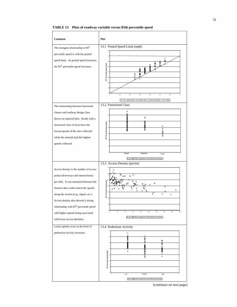
TABLE 13 Plots of roadway variable versus 85th percentile speed

Comment

Plot

The strongest relationship to 85th

percentile speed is with the posted

speed limit. As posted speed increases

the 85th percentile speed increases.

13.1 Posted Speed Limit (mph)

0

10

20

30

40

50

60

70

80

0 10 20 30 40 50 60 70

Local Collectors Arterial, C&G Arterial, Shoulder SL = 85th

85 th P

erce

nti

le S

pee

d (

mp

h)

The relationship between functional

classes and roadway design class

shows an expected plot. Roads with a

functional class of local have the

lowest speeds of the sites collected

while the arterials had the highest

speeds collected.

13.2 Functional Class

0

10

20

30

40

50

60

70

0 Arterial Collectors Local 4

Local Collectors Arterial, C&G Arterial, Shoulder

85 th P

erce

nti

le S

pee

d (

mp

h)

Access density is the number of access

points (driveways and intersections)

per mile. It was measured between the

features that could control the speeds

along the section (e.g., signal, etc.).

Access density also showed a strong

relationship with 85th percentile speed

with higher speeds being associated

with lower access densities.

13.3 Access Density (pts/mi)

0

10

20

30

40

50

60

70

0 20 40 60 80 100 120 140 160 180

85 th P

erce

nti

le S

pee

d (

mp

h)

Local Collectors Arterial, C&G Arterial, Shoulders

Lower speeds occur as the level of

pedestrian activity increases.

13.4 Pedestrian Activity

0

10

20

30

40

50

60

70

0 Low Medium High 4


85 th P

erce

nti

le S

pee

d (

mp

h)

31


TABLE 13 (Continued)

Comment

Plot

13.5 Center Line Markings

0

10

20

30

40

50

60

70

0 Center line marked Center line not marked 3

85 th P

erce

nti

le S

pee

d (

mp

h)


The absence of either centerline

markings or edgeline markings is

associated with lower speeds.

13.6 Edge Line Markings

0

10

20

30

40

50

60

70

0 1 2 3

Edge Line Markings (1=yes, 2=no)

85th

Per

cen

tile

Sp

eed

(m

ph

)

Local Collectors Arterial, C&G Arterial, Shoulder When on-street parking is permitted,

speeds are lower.

13.7 Parking

0

10

20

30

40

50

60

70

0 Parking permitted Parking not permitted 3

85 th P

erce

nti

le S

pee

d (

mp

h)

Local Collectors Arterial, C&G Arterial, Shoulder When no median is present, speeds are

slightly lower than when a raised,

depressed, or TWLTL is present with a

few exceptions.

13.8 Median Type

0

10

20

30

40

50

60

70

Raised Depressed Two Way with Left Turn Lane

85 th P

erce

nti

le S

pee

d (

mp

h)


None

32


Comment

Plot

As the distances between features that have

influence on a driver’s speed, such as a signal

or sharp horizontal curve, increase, speeds

increase.

13.9 Distance between Controls

0

10

20

30

40

50

60

70

0.0 0.5 1.0 1.5 2.0 2.5

85 th P

erce

nti

le S

pee

d (

mp

h)

Local Collectors Arterial, C&G Arterial, Shoulders Speeds on roadways with shoulders that had

widths equal to or greater than 6 ft had

speeds above 50 mph (with one exception).

Speeds on roadways with shoulders between

0 and 4 ft also had speeds up to 50 mph with

most being less than the speeds observed on

the roadways with wider shoulders. Roadways

with curb and gutter had speeds across the

entire range seen on roadways with shoulders

(25 to almost 60 mph). There is no evidence

that the presence of curb and gutter results

in lower speeds for a facility.

13.10 Shoulder Width

0

10

20

30

40

50

60

70

-4 Curb and

gutter

0 2 4 6 8 10 12 14 Feet

85 th

Per

cen

tile

Sp

eed

(m

ph)


Higher signal densities are associated with

lower speeds.

13.11 Signal Density

0

10

20

30

40

50

60

70

0.0 1.0 2.0 3.0 4.0 5.0 6.0 signals/mi

85 th P

erce

nti

le S

pee

d (

mp

h)

Local Collectors Arterial, C&G Arterial, Shoulder Fewer lower speeds are associated with larger

total pavement widths.

13.12 Total Pavement Width

0

10

20

30

40

50

60

70

0 20 40 60 80 100 120 140 Feet

85 th P

erce

nti

le S

pee

d (

mp

h)




Comment

Plot

Fewer lower speeds are associated with

the higher median widths.

13.13 Median Width

0

10

20

30

40

50

60

70

0 10 20 30 40 50 60 70 80 90 Feet

85 th P

erce

nti

le S

pee

d (

mp

h)


A wide range of speeds were recorded

for each roadside environment class.

13.14 Roadside Environment @ 2 ft

0

10

20

30

40

50

60

70

-1 0 1 2 3 4 5

Roadside Environment @ 2 ft (0=clear, 1=yielding objects, 2=combination of yielding and isolated rigid, 3=isolated rigid objects only, 4=many or continuous rigid objects)

85th

Per

cen

tile

Sp

eed

(m

ph

)

Local Collectors Arterial, C&G Arterial, Shoulder 13.14 Roadside Environment @ 10 ft

0

10

20

30

40

50

60

70

-1 0 1 2 3 4 5

Roadside Environment @ 10 ft (0=clear, 1=yielding objects, 2=combination of yielding and isolated rigid, 3=isolated rigid objects only, 4=many or continuous rigid objects)

85th

Per

cen

tile

Sp

eed

(m

ph

)

Local Collectors Arterial, C&G Arterial, Shoulder This plot shows no relationship

between lane width and speed.

13.15 Lane Width

0

10

20

30

40

50

60

70

0 5 10 15 20 25 30 Feet

85 th P

erce

nti

le S

pee

d (

mp

h)


34

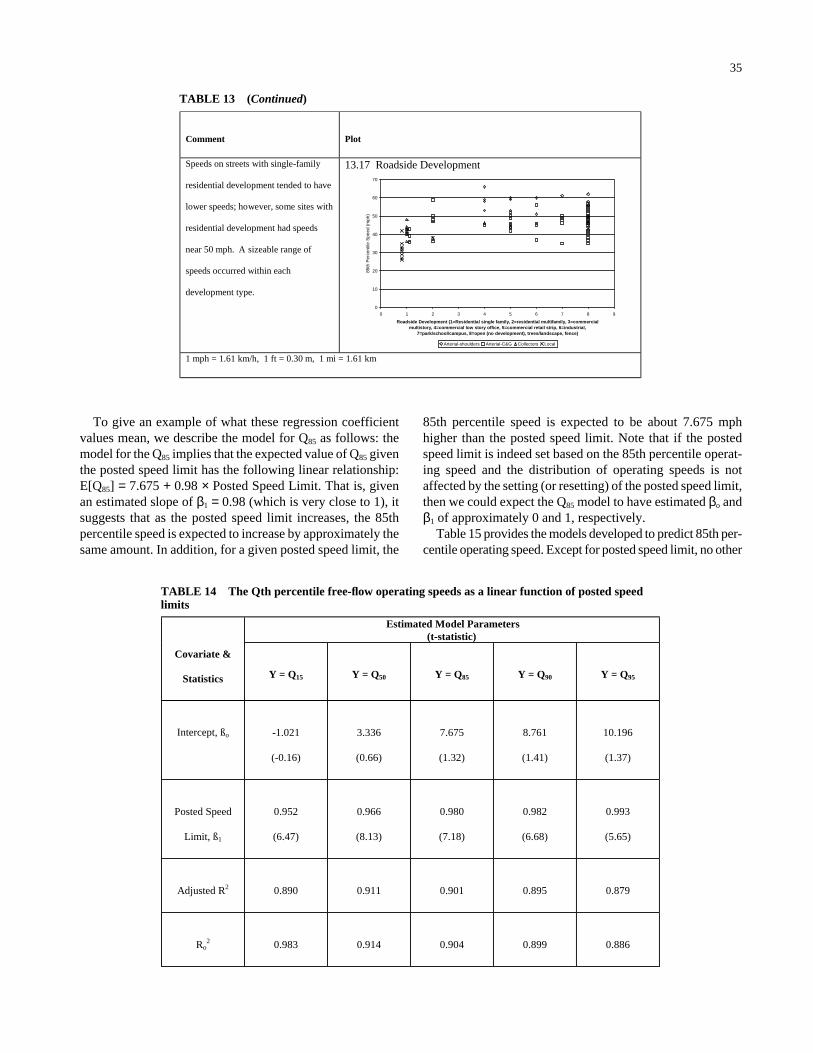
To give an example of what these regression coefficientvalues mean, we describe the model for Q85 as follows: themodel for the Q85 implies that the expected value of Q85 giventhe posted speed limit has the following linear relationship:E[Q85] = 7.675 + 0.98 × Posted Speed Limit. That is, givenan estimated slope of β1 = 0.98 (which is very close to 1), itsuggests that as the posted speed limit increases, the 85thpercentile speed is expected to increase by approximately thesame amount. In addition, for a given posted speed limit, the

35

85th percentile speed is expected to be about 7.675 mphhigher than the posted speed limit. Note that if the postedspeed limit is indeed set based on the 85th percentile operat-ing speed and the distribution of operating speeds is notaffected by the setting (or resetting) of the posted speed limit,then we could expect the Q85 model to have estimated βo andβ1 of approximately 0 and 1, respectively.

Table 15 provides the models developed to predict 85th per-centile operating speed. Except for posted speed limit, no other


Comment

Plot

Speeds on streets with single-family

residential development tended to have

lower speeds; however, some sites with

residential development had speeds

near 50 mph. A sizeable range of

speeds occurred within each

development type.

13.17 Roadside Development

0

10

20

30

40

50

60

70

0 1 2 3 4 5 6 7 8 9

Roadside Development (1=Residential single family, 2=residential multifamily, 3=commercial multistory, 4=commercial low story office, 5=commercial retail strip, 6=industrial,

7=park/school/campus, 8=open (no development), trees/landscape, fence)

85th

Per

cent

ile S

peed

(m

ph)

Arterial-shoulders Arterial-C&G Collectors Local 1 mph = 1.61 km/h, 1 ft = 0.30 m, 1 mi = 1.61 km

TABLE 14 The Qth percentile free-flow operating speeds as a linear function of posted speedlimits

Estimated Model Parameters(t-statistic)

Covariate &

Statistics

Y = Q15

Y = Q50

Y = Q85

Y = Q90

Y = Q95

Intercept, ßo

-1.021

(-0.16)

3.336

(0.66)

7.675

(1.32)

8.761

(1.41)

10.196

(1.37)

Posted Speed

Limit, ß1

0.952

(6.47)

0.966

(8.13)

0.980

(7.18)

0.982

(6.68)

0.993

(5.65)

Adjusted R2

0.890

0.911

0.901

0.895

0.879

Ro2

0.983

0.914

0.904

0.899

0.886

roadway variables were statistically significant at a 5 percentalpha level. The only variable that had a t-statistic greater than1 was access density, which had a t-value of ±1.31, corre-sponding to approximately a 20 percent alpha level. Figure 1shows a scatter plot of the relationship, with the sizes of theovals representing the standard deviation for the site. Figure 2provides a graphic illustration of the regression equations.

Analysis by Roadway Functional Class

The 78 sites were divided into four functional classes:suburban/urban (S/U) arterial, S/U collector, S/U local, andrural arterial. The number of sites available in each of thefour functional classes for analysis is 35, 21, 13, and 9,respectively. Table 16 presents modeling results from linearregressions. Figure 3 provides a graphical illustration of theregression equations.

The posted speed limit continues to exhibit a strong statisti-cal relationship with the 85th percentile speed for the S/U arte-rial and rural arterial classes. For S/U arterial, the estimatedslope parameter of 0.963 suggests that a 1-mph (1.6-km/h)increase in the posted speed limit is likely to be associatedwith about a 1-mph (1.6-km/h) increase in the expected 85thpercentile operating speed. On the other hand, the estimatedslope parameter in the rural arterial model drops significantlyto 0.517, indicating that a 1-mph (1.6-km/h) increase in theposted speed limit for rural arterial is likely to be associatedwith a 2-mph (3.2-km/h) increase in the expected 85th per-centile operating speed. Note, however, given the small sam-ple size for the rural arterial (n = 9), this interpretation shouldbe used with caution.

Based on the model goodness of fit, the division by func-tional class results in a relatively weak statistical relationshipbetween the posted speed and operating speed for S/U col-lector and S/U local roads. The weak relationships are due

36

mainly to the narrow posted speed limit range within eachfunctional class and smaller sample size.

To explore whether any of the roadway variables could helpto improve the models in Table 15, a stepwise forward selec-tion regression procedure was used. No other roadway vari-able was statistically significant (even at a 20 percent alphalevel) in terms of providing additional explaining power on thevariation of the 85th percentile speed. The only models thatcome close to meeting the 30 percent alpha level are presentedin Table 17. Both models are for the S/U collector. Oneincludes the access density as an additional explanatory vari-able, and the other includes the median type. The coefficientof the access density in the first model seems to be quite con-sistent with that obtained in the model presented in Table 15,where calibration was performed with the combined data set.The coefficient for the type of median is not as logical. Onecould expect that the speeds would be lower on a roadwaywhere vehicles turning left are stopping in the travel lane andthat the speeds could increase once a TWLTL is provided tostore these vehicles. For the data set available, only two siteshad a TWLTL, which may be insufficient to accurately cap-ture the speed relationship between roads with or without left-turn treatments.

Analysis for Sites with a 30-mph (48.3-km/h)Posted Speed Limit

As can be seen from Figure 4, sites with a 30-mph (48.3-km/h) posted speed limit experienced relatively more varia-tion in the 85th percentile operating speed as compared withthe range present at other posted speed groups. It would beinteresting to know if any of the roadway variables couldexplain this variation in a statistically significant way. Novariable was found to pass the 20 percent alpha level. Onlyone variable comes close to the 30 percent alpha level: vehi-

TABLE 15 Free-flow 85th percentile operating speed as a linear function of posted speed limitsand other variables


Model #

Intercept

Posted Speed

Limit (mph)

Access Density per Mile

(for PSL≤45 mph)

Ro2

1

7.675

(1.32)

0.980

(7.18)

0.904

2

16.089

(2.03)

0.831

(5.26)

-0.054

(-1.31)

0.923

cle parking along the street. Table 18 shows this model. Itseems to suggest that among the 30-mph (48.3-km/h) sites,those with vehicles parking along the street tend to have alower 85th percentile operating speed by about 7.5 mph(12.1 km/h) when compared with other sites that do not havevehicles parking on the side. Again, because of the low t-value,this interpretation should be used with caution.

Cluster Analysis

Given that we were unable to establish good statisticalrelationships for all considered roadway variables with thecurrent sample size (except for the posted speed limit), a clus-ter analysis was performed to see if the project team could gainadditional insights over educated inspection and judgment byclassifying roadways quantitatively according to “similarities”of their attributes and perceived influences of these attributeson operating speeds. Cluster analysis is known to offer sev-eral advantages over a manual grouping process. For example,it usually provides a more objective and consistent way ofgrouping objects, particularly for objects with more than threefeatures or dimensions. Appendix E, Field Studies, containsdetails on the cluster analysis. The analysis resulted in a seven-cluster model. The following were the noteworthy features

37

found within the analysis: pedestrian activity, parking, use ofcenterline markings, median treatment, roadside development,area type, and signal density.

SELECTION OF DESIGN SPEED VALUE

Simplified, the process of designing a roadway beginswith selecting a speed called the design speed. Then, usingthis selected design speed in conjunction with a series oftables and figures, the appropriate design criteria are chosenfor the roadway features. For example, once a value for designspeed has been chosen, it is used to determine the allowablehorizontal curve radii, whether curb and gutter should beused, and other roadway elements. The elements are thenassembled to develop the roadway cross section and the designplans used in construction.

Selecting a Design Speed Value

Methods used to select a design speed value were identi-fied from the AASHTO guidelines, from state agencies’manuals, from a mailout survey, and from the literature forinternational practices. These reviews demonstrate that sub-stantial variations exist in how design speeds are selected.

Figure 1. Scatter plot of the 85th percentile operating speed by area type, roadway class, andposted speed limit.

AASHTO Guidelines

In the 1930s, U.S. Bureau of Public Roads engineers rec-ommended that the design speed of a future highway shouldbe the speed that only 5 percent or possibly 2 percent of thedrivers will exceed after the road is built. In other words,the Bureau engineers were recommending design speedvalues equivalent to the anticipated 95th or 98th percentileoperating speeds. Quantitative guidelines for design speedbased on functional classification, rural versus urban, andterrain type (level, rolling, and mountainous) can be foundin Chapters 5, 6, 7, and 8 of the 2001 Green Book (17). Forexample, AASHTO provides quantitative guidance for rec-ommended design speeds for rural arterials by terrain type onpage 448 in the 2001 Green Book. AASHTO also discusses

38

other factors—such as operating speed, adjacent lane use,and safety—but provides little, if any, quantitative guidancerelated to how such factors should be considered or impactthe selection process of a design speed value.

United States Practices

The results of the mailout survey conducted as part of theNCHRP 15-18 research project provide interesting insightinto how the design speed value is selected. For instance,while most agencies use either the AASHTO Green Bookor their state design manual in considering the traditionalfactors—such as functional classification and terrain, to namea few—some agencies also consider legislatively mandated

0

5

10

15

20

25

30

35

40

45

0 20 40 60 80 100 120 140 160 180

Access Density (pts/mi)

Sp

eed

(m

ph

)

PSL=25, field data PSL=30, field data

PSL=25, reg PSL=30, reg

(a) Local

0

10

20

30

40

50

60

0 20 40 60 80 100 120 140 160 180


Sp

eed

(m

ph

)



PSL=45, field data PSL=30, regression

PSL=35, regression PSL=40, regression

(b) Collectors

Figure 2. Plots of regression equations using posted speed limit and access density.

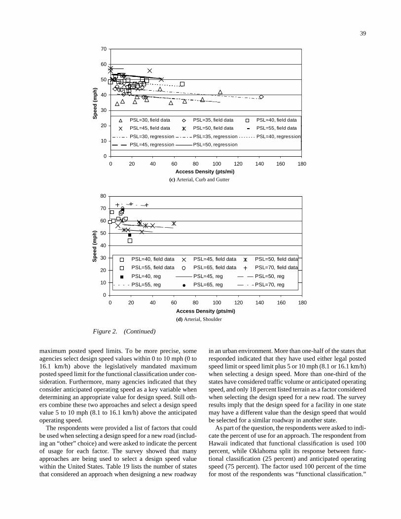
maximum posted speed limits. To be more precise, someagencies select design speed values within 0 to 10 mph (0 to16.1 km/h) above the legislatively mandated maximumposted speed limit for the functional classification under con-sideration. Furthermore, many agencies indicated that theyconsider anticipated operating speed as a key variable whendetermining an appropriate value for design speed. Still oth-ers combine these two approaches and select a design speedvalue 5 to 10 mph (8.1 to 16.1 km/h) above the anticipatedoperating speed.

The respondents were provided a list of factors that couldbe used when selecting a design speed for a new road (includ-ing an “other” choice) and were asked to indicate the percentof usage for each factor. The survey showed that manyapproaches are being used to select a design speed valuewithin the United States. Table 19 lists the number of statesthat considered an approach when designing a new roadway

39

in an urban environment. More than one-half of the states thatresponded indicated that they have used either legal postedspeed limit or speed limit plus 5 or 10 mph (8.1 or 16.1 km/h)when selecting a design speed. More than one-third of thestates have considered traffic volume or anticipated operatingspeed, and only 18 percent listed terrain as a factor consideredwhen selecting the design speed for a new road. The surveyresults imply that the design speed for a facility in one statemay have a different value than the design speed that wouldbe selected for a similar roadway in another state.

As part of the question, the respondents were asked to indi-cate the percent of use for an approach. The respondent fromHawaii indicated that functional classification is used 100percent, while Oklahoma split its response between func-tional classification (25 percent) and anticipated operatingspeed (75 percent). The factor used 100 percent of the timefor most of the respondents was “functional classification.”

0

10

20

30

40

50

60

70

0 20 40 60 80 100 120 140 160 180


Sp

eed

(m

ph

)

PSL=30, field data PSL=35, field data PSL=40, field data


PSL=30, regression PSL=35, regression PSL=40, regression

PSL=45, regression PSL=50, regression

(c) Arterial, Curb and Gutter

0

10

20

30

40

50

60

70

80

0 20 40 60 80 100 120 140 160 180


Sp

eed

(m

ph

)



PSL=40, reg PSL=45, reg PSL=50, reg

PSL=55, reg PSL=65, reg PSL=70, reg

(d) Arterial, Shoulder

Figure 2. (Continued)

The percent-of-use answers were used to weight the numberof responses. The order of the factors most used, from high-est to lowest, was as follows:

• functional classification, • legal speed limit (legislative or maximum value), • legal speed limit plus 5 or 10 mph (8.1 to 16.1 km/h), • traffic volume, and • anticipated operating speed.

Other factors occasionally considered when selecting thedesign speed for a new road include terrain, development,costs, and consistency within a corridor.

International Practices

Krammes et al. (33) reviewed the design practices in sevencountries (Australia, Canada, France, Germany, Great Britain,and Switzerland) to determine their procedures for selectingand applying a selected design speed value. At one time,most of the countries’ policies on design speed were identi-cal to current U.S. policy. Procedures for selecting a designspeed are still similar to U.S. practice (i.e., based on the classof the roadway, rural versus urban, and terrain). However,during the last 20 years several countries have refined theirprocedures for applying design speed.

40

Australia, France, Great Britain, Germany, and Switzerlandgive more formal and explicit consideration of operatingspeeds than does AASHTO policy. Although the details vary,these countries include feedback loops in the alignment designprocedures to identify and resolve operating speed incon-sistencies. In all countries reviewed, design speed is used todetermine minimum horizontal curve radii for the preliminaryalignment design. In most countries, however, superelevationrates and sight distances are based on the estimated 85th per-centile speed when it exceeds the design speed.

In addition, several countries provide quantitative guide-lines on the radii of successive horizontal alignment features.France and Germany specify the minimum radius followinglong tangents. Germany also has a comprehensive guidelineindicating acceptable and unacceptable ranges for the radii ofsuccessive curves.

Which Factors Make a Difference?

Table 20 lists the factors that are used to select design speedfrom the three methods reviewed in this project: AASHTOpolicy, state DOT practices, and international practices. If onebelieves that the design of the roadway (as represented by thedesign speed of the road) affects the operating speed of a facil-ity (as represented by the 85th percentile speed), then the useof different design speeds should result in different operatingspeeds. Because functional class, rural versus urban, and ter-rain affect the design speed selected, then different operatingspeeds should be associated with differences in these factors. If

TABLE 16 The 85th percentile free-flow operating speed as a linear function of posted speedlimits by functional class

Estimated Model Parameters (t-statistic)

Covariate and

Statistics

S/U Arterial

S/U Collector

S/U Local

Rural Arterial

Intercept

8.666

(0.92)

21.131

(1.05)

10.315

(0.19)

36.453

(3.41)

Posted Speed Limit

0.963

(4.50)

0.639

(1.14)

0.776

(0.41)

0.517

(3.02)

Ro2

0.86

0.41

0.14

0.81

Sample Size (n)

35

21

13

9

S/U = suburban/urban.

differences in these factors are not associated with differencesin operating speed, then one should question whether theyshould play a role in selecting the design speed of the highway.

Of course, the use of the three factors (functional class,rural versus urban, and terrain) to select design speed may bejustified based on reasons other than anticipated operatingspeed. The anticipated posted speed for the facility or theexpected traffic volumes may need to be considered. Also, theuse of lower design speeds on mountainous terrain may bejustified by cost considerations and by driver expectancies.

Functional Classification/Urban versus Rural

Figure 5 shows the cumulative speed distribution for urban/suburban arterials, collectors, and local streets. Most of thedata were collected during the summer of 2000, with 35 ofthe 69 arterial sites collected in Texas during 1998 and 1999.

41

At each site, spot speeds were collected on a tangent sectionof the roadway away from potential influences such as signalsor horizontal curves. The remaining sites were in Boston,Little Rock, Nashville, Portland, St Louis, and the followingTexas cities: Bryan, Corpus Christi, College Station, Hous-ton, San Antonio, and Waco. Vehicles not at free-flow speed(defined as having less than a 5-s headway between vehicles)were removed from the data sets. Table 21 lists the speed val-ues for the percentages previously suggested as the thresholdthat could be used for selecting a design speed. As expected,there are noticeable differences in operating speeds for local,collector, and arterial streets.

Terrain

While the authors did not have speed data by terrain typefor freeways available, they did have access to data for rural

0

10

20

30

40

50

60

70

80

0 10 20 30 40 50 60 70

Posted Speed Limit (mph)

85th

Per

cen

tile

Sp

eed

(m

ph

)

Local SL = 85th Regression: Local

0

10

20

30

40

50

60

70

80

0 10 20 30 40 50 60 70


85th

Per

cen

tile

Sp

eed

(m

ph

)

Collectors SL = 85th Reg: Collector

(a) Local

(b) Collector

Figure 3. Plots of regression equations using posted speed limit. (continued on next page)

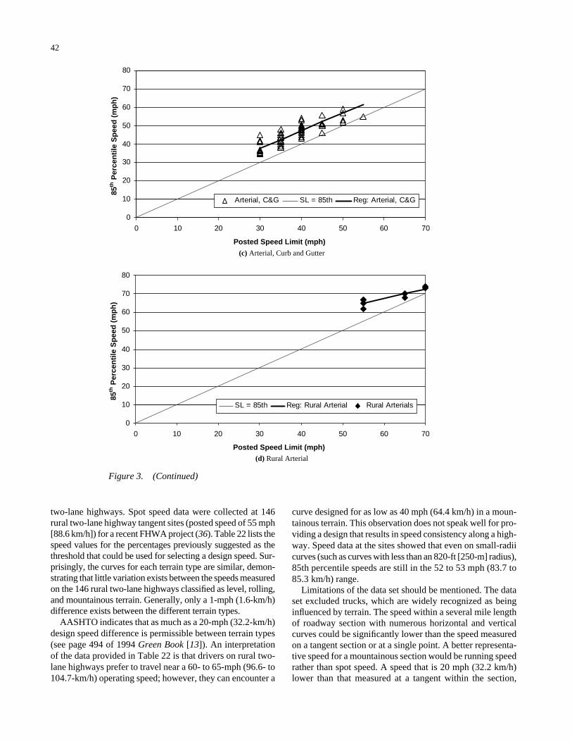
two-lane highways. Spot speed data were collected at 146rural two-lane highway tangent sites (posted speed of 55 mph[88.6 km/h]) for a recent FHWA project (36). Table 22 lists thespeed values for the percentages previously suggested as thethreshold that could be used for selecting a design speed. Sur-prisingly, the curves for each terrain type are similar, demon-strating that little variation exists between the speeds measuredon the 146 rural two-lane highways classified as level, rolling,and mountainous terrain. Generally, only a 1-mph (1.6-km/h)difference exists between the different terrain types.

AASHTO indicates that as much as a 20-mph (32.2-km/h)design speed difference is permissible between terrain types(see page 494 of 1994 Green Book [13]). An interpretationof the data provided in Table 22 is that drivers on rural two-lane highways prefer to travel near a 60- to 65-mph (96.6- to104.7-km/h) operating speed; however, they can encounter a

42

curve designed for as low as 40 mph (64.4 km/h) in a moun-tainous terrain. This observation does not speak well for pro-viding a design that results in speed consistency along a high-way. Speed data at the sites showed that even on small-radiicurves (such as curves with less than an 820-ft [250-m] radius),85th percentile speeds are still in the 52 to 53 mph (83.7 to85.3 km/h) range.

Limitations of the data set should be mentioned. The dataset excluded trucks, which are widely recognized as beinginfluenced by terrain. The speed within a several mile lengthof roadway section with numerous horizontal and verticalcurves could be significantly lower than the speed measuredon a tangent section or at a single point. A better representa-tive speed for a mountainous section would be running speedrather than spot speed. A speed that is 20 mph (32.2 km/h)lower than that measured at a tangent within the section,

0

10

20

30

40

50

60

70

80

0 10 20 30 40 50 60 70


85th

Per

cen

tile

Sp

eed

(m

ph

)

Arterial, C&G SL = 85th Reg: Arterial, C&G

(c) Arterial, Curb and Gutter

0

10

20

30

40

50

60

70

80

0 10 20 30 40 50 60 70


85th

Per

cen

tile

Sp

eed

(m

ph

)

SL = 85th Reg: Rural Arterial Rural Arterials

(d) Rural Arterial

Figure 3. (Continued)

however, would not be expected. Therefore, the analysis indi-cates that the use of terrain to select an appropriate designspeed that would result in a design that promotes speed con-sistency should be investigated. If predictable operatingspeeds along a two-lane rural highway are desired, the dataindicate that the type of terrain would not be a valued vari-able in terms of predicting speed variability.

Potential Solutions

Potential solutions to the concerns discussed previouslyinclude limiting the range of design speed values availablewithin each functional class, rural versus urban, or terrain type;

43

using anticipated posted or operating speed (or using antic-ipated posted or operating speed plus a preset incrementalincrease); incorporating a feedback loop that would checkthe predicted speed along an alignment; or managing speedson the tangent section by controlling the tangent length. Fol-lowing is a brief overview of the two potential solutions thathold the most promise.

Consideration of Anticipated Posted or Operating Speed

Several states use the anticipated posted, anticipated oper-ating, or the anticipated posted or operating speed plus 5 or

TABLE 17 The 85th percentile free-flow operating speeds as a linear function of posted speedlimits and other variables for suburban/urban collectors


Covariate & Statistics

Suburban/Urban Collector

Suburban/Urban Collector

Intercept

14.715

(1.67)

22.489

(1.47)

Posted Speed Limit

0.400

(1.59)

0.674

(1.66)

Access Density per Mile

(for PSL ≤ 45 mph)

-0.059

(1.05)

Median Type = Two Way Left

Turn Lane

-7.860

(-1.10)

Median Type = No Median

-2.593

(-0.56)

Ro2

0.586

0.583

Sample Size (n)

22

22

10 mph (8.1 or 16.1 km/h). A resulting benefit of this approachis that it ensures that the posted speed will not exceed thedesign speed—a liability concern expressed previously. Apotential for discontinuity exists between states that havelimited their freeway speeds to 55 mph (88.6 km/h) and thosewith 65- or 70-mph (104.7- or 112.7-km/h) speed limits. Ifall states adopt the procedure to set design speed at antici-pated posted speed plus 5 mph (8.1 km/h), then state A witha legislatively mandated speed of 55 mph (88.6 km/h) wouldhave a design speed of 60 mph (96.6 km/h) while state Bwith a legislatively mandated maximum speed of 70 mph(112.7 km/h) would have a design speed of 75 mph (120.8km/h). In other words, there could be a 15-mph (24.2-km/h)difference in design speeds between neighboring states for asimilar functional class road (e.g., freeways).

44

A challenge with this approach is the selection of theincrement above the anticipated posted or operating speed.This increment can represent a “safety factor” for drivers ora “cushion” between the current anticipated posted speed anda higher, perhaps legislatively allowed, future posted speed.As a safety factor, is setting sight distances for 5 or 10 mph(8.1 or 16.1 km/h) greater than the posted or operating speedsufficient? As a cushion, is 5 or 10 mph (8.1 or 16.1 km/h)sufficient to anticipate future changes in posted speeds? Areview of recent changes in speed limit laws showed that the5 or 10 mph (8.1 or 16.1 km/h) currently used by some stateswould not be adequate for rural areas. In Texas, four legisla-tive actions have changed the rural speeds limits from 55 to75 mph (88.6 to 120.8 km/h) for certain areas. Therefore,debate is needed on what should be considered as an accept-able cushion for potential speed increases.

Feedback Loop with a Speed Prediction Model

A method for ensuring that operating speeds are consid-ered within the design is to use a speed prediction model witha feedback loop. The method would predict the operatingspeed along an alignment and then compare the predictedspeed with the design speed. Krammes et al. (33) notes thatseveral countries (Australia, England, France, Germany, andSwitzerland) give more formal and explicit consideration to operating speeds than AASHTO policy does. The basicapproach was provided as follows:

• Design a preliminary alignment based on the selecteddesign speed.

• Estimate 85th percentile speeds on that alignment.• Check for large differences between 85th percentile

speeds on successive curves.• Revise the alignment to reduce these differences to

acceptable levels.

Figure 4. Relationship between the 85thpercentile operating speed and posted speedlimit (with sampling variations).

TABLE 18 A model of the 85th percentile free-flow operating speeds for sites with a 30-mph posted speed limit


Intercept

Parking Along

Street = Yes

RModel

Type

o2

Sample Size

Model for 30 mph

sites

40.401

(7.74)

-7.565

(-0.99)

0.50

15

45

TABLE 19 Approaches used by states

Approach

Number of States

(maximum of 40)

%

Functional Classification

36

90

Either Legal Speed Limit or Limit + Value

23

58

Legal Speed Limit

17

43

Legal Speed Limit plus 5 or 10 mph

11

28

Traffic Volume

15

38

Anticipated Operating Speed

15

38

Terrain

7

18

TABLE 20 Factors used to select design speed

AASHTO Policy

State DOT Survey

International Practices

Functional classification

Rural versus urban

Terrain type

Functional classification

Legal speed limit

Legal speed limit plus a value (e.g., 5 or 10 mph

[8.1 to 16.1 km/h])

Anticipated volume

Anticipated operating speed

Terrain type

Development

Costs

Consistency

Anticipated operating speed

Feedback loop

The Federal Highway Administration is developing theInteractive Highway Safety Design Model (IHSDM) in anattempt to marshal available knowledge about safety into amore useful form for highway planners and designers (52).One of the IHSDM modules is the Design Consistency Mod-ule. It provides information on the extent to which a road-way design conforms with drivers’ expectations. The primarymechanism for assessing design consistency is a speed-profilemodel that estimates 85th percentile speeds at each pointalong a roadway. Potential consistency problems for whichalignment elements will be flagged include large differencesbetween the assumed design speed and estimated 85th per-

46

centile speed and large changes in 85th percentile speedsbetween successive alignment elements.

OPERATING SPEED AND POSTED SPEEDRELATIONSHIPS

It is generally acknowledged that 85th percentile operatingspeeds exceed posted speeds (15, 22, 33, 36, 38, 43, 53). Manyof these reports have also demonstrated that the 50th percentileoperating speed either is near or exceeds the posted speedlimit. Data available within the NCHRP 15-18 project also

0

10

20

30

40

50

60

70

80

90

100

0 10 20 30 40 50 60 70 80 90

85th Percentile Speed (mph)

Cu

mu

lati

ve D

istr

ibu

tio

n (

%)

Arterials, 69 sites

Collectors, 20 sites

Locals, 13 sites

Figure 5. Distribution of 85th percentile speeds on tangent sections of urban andsuburban roadways by functional class.

TABLE 21 Speed values by functional class for urban and suburban streets

Functional

Class

Number of

Sites

Number of

Individual

Readings

85th Percentile

Speed

mph (km/h)

95th Percentile

Speed

mph (km/h)

98th Percentile

Speed

mph (km/h)

Arterials (all)

69

16425

60 (96.6)

68 (109.5)

71 (114.3)

Collectors

20

5961

44 (70.8)

49 (78.9)

53 (85.3)

Local

13

3000

34 (54.7)

39 (62.8)

42 (67.6)

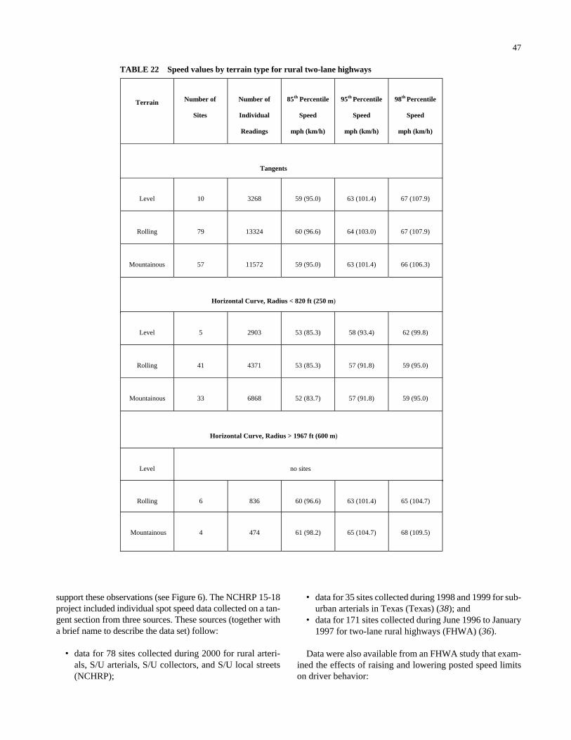
support these observations (see Figure 6). The NCHRP 15-18project included individual spot speed data collected on a tan-gent section from three sources. These sources (together witha brief name to describe the data set) follow:

• data for 78 sites collected during 2000 for rural arteri-als, S/U arterials, S/U collectors, and S/U local streets(NCHRP);

47

• data for 35 sites collected during 1998 and 1999 for sub-urban arterials in Texas (Texas) (38); and

• data for 171 sites collected during June 1996 to January1997 for two-lane rural highways (FHWA) (36).

Data were also available from an FHWA study that exam-ined the effects of raising and lowering posted speed limitson driver behavior:

TABLE 22 Speed values by terrain type for rural two-lane highways

Terrain

Number of

Sites

Number of

Individual

Readings

85th Percentile

Speed

mph (km/h)

95th Percentile

Speed

mph (km/h)

98th Percentile

Speed

mph (km/h)

Tangents

Level

10

3268

59 (95.0)

63 (101.4)

67 (107.9)

Rolling

79

13324

60 (96.6)

64 (103.0)

67 (107.9)

Mountainous

57

11572

59 (95.0)

63 (101.4)

66 (106.3)

Horizontal Curve, Radius < 820 ft (250 m)

Level

5

2903

53 (85.3)

58 (93.4)

62 (99.8)

Rolling

41

4371

53 (85.3)

57 (91.8)

59 (95.0)

Mountainous

33

6868

52 (83.7)

57 (91.8)

59 (95.0)

Horizontal Curve, Radius > 1967 ft (600 m)

Level

no sites

Rolling

6

836

60 (96.6)

63 (101.4)

65 (104.7)

Mountainous

4

474

61 (98.2)

65 (104.7)

68 (109.5)

• data for 98 sites collected between June 1986 and July1989 on nonlimited access highways (Parker) (53).

The data within the NCHRP and Texas databases followtrends similar to those of the Parker data. In both those setsof data, the 85th percentile speeds at most sites exceed theposted speed. Parker determined that the typical posted speedlimit represented the 43rd percentile speed. Statistics fromthe NCHRP, Texas, and FHWA data sets on the percentile ofvehicles that travel at various speeds (including the postedspeed limit) are given in Table 23.

Figure 6 and Table 23 illustrate differences between ruraltwo-lane highways and S/U roadways. In most situations,posted speeds represent a higher percentile value in ruralareas than S/U areas. The only exception is the rural, arterialsubdivision for the nine sites collected within this NCHRPstudy. The results for these nine sites (37th percentile speedequals posted speed) is heavily influenced by two Portlandsites that have operating speeds in excess of 65 mph (104.6km/h) while speed limits are 55 mph (88.5 km/h). Whenthese two sites are eliminated, the result goes to the 48th per-centile, which is more in line with the findings for the otherrural categories.

Rural two-lane highway sites accounted for most of thesites having 85th percentile speed values lower than theposted speed. Figure 6 shows that only one S/U local streetsite and one S/U arterial site had 85th percentile speeds lessthan the posted speed and that no S/U collector site did.Several of the rural two-lane highway sites had 85th per-centile speeds less than the posted speed.

In addition to providing information on the percentilespeed that equals the posted speed, Table 23 provides infor-mation on the percentile speed for posted speed plus 5 mph(8.1 km/h) and plus 10 mph (16.1 km/h). For rural roadswhere the functional classification is principal arterial (repre-

48

senting 36 sites in Washington), 72 percent of the free-flowvehicles were at the posted speed limit. For those roads, postedspeed limit was either 50 or 55 mph (80.5 or 88.5 km/h). Atotal of 90 percent of the free-flow vehicles were at the postedspeed limit plus 5 mph (8.1 km/h) (i.e, 55 or 60 mph [88.5or 96.6 km/h]). When the posted speed limit plus 10 mph(16.1 km/h) is used, the percent of vehicles at or below thatspeed goes to 98 percent. For those 36 sites, almost all thevehicles on the roadways were at or below posted speed plus10 mph (16.1 km/h). For all the rural classes, over 90 percentand in most cases over 97 percent of the vehicles on the road-ways are within 10 mph (16.1 km/h) of the speed limit.

S/U classes show a different speed pattern. Overall, thereare greater speed differences between the operating speedand the posted speed limit for the sites studied. Local streetshad speeds that were the closest to the posted speed limit,with 96 percent of the vehicles at or below speed limit plus10 mph (16.1 km/h). Collectors had the poorest perfor-mance, with only 86 percent of the measured free-flowvehicles being at or below speed limit plus 10 mph (16.1km/h). Only 23 percent of the free-flow vehicles on collec-tors were at the posted speed limit.

Table 24 lists the percentile speed that equals speed limit,speed limit plus 5 mph (8.1 km/h), and speed limit plus 10 mph (16.1 km/h) grouped by the speed limit for the road-way. For rural nonfreeway facilities, speed limit plus 10 mph(16.1 km/h) would include almost all vehicles on the road-ways. For suburban/urban areas, speed limit plus 10 mph(16.1 km/h) would only include between 86 and 95 percentof the vehicles on the roadways. A much larger percentageof vehicles exceed the speed limit on suburban/urban non-freeway roadways than on rural nonfreeway roadways. Forthe 30-, 35-, and 40-mph (48.3-, 56.3-, and 64.4-km/h) speedlimits, only 28, 22, and 32 percent, respectively, of the vehi-cles on the road were at or below the posted speed limit.

0

10

20

30

40

50

60

70

80

0 10 20 30 40 50 60 70 80


85th

Per

cen

tile

Sp

eed

(m

ph

)

Rural ArterialsS/U ArterialsS/U CollectorsS/U LocalSL = 85th

Figure 6. 85th percentile speed versus posted speed for NCHRP,Texas, and FHWA data.

TABLE 23 Percentile speed compared with posted speed

Percentile at or below

Given Speed*

Data

Source

Development,

Functional Class

(Posted Speed Range)

Speed

Limit

Speed

Limit

Plus

5 mph

Speed

Limit

Plus

10 mph

Number of Sites

(location)

NCHRP

Rural, Arterial

(55 to 70 mph)

37**

70

91

9 (near College Station,

Portland, and St. Louis)

FHWA

Rural, Minor Arterial

(55 mph)

59

87

99

9 (Washington)

FHWA

Rural, Principal Arterial

(50 to 55 mph)

72

90

98

36 (Washington)

FHWA

Rural, no class given

(50 to 70 mph)

64

86

97

126 (Minnesota, New York,

Oregon, Pennsylvania, Texas)

Texas

Suburban/Urban, Arterial

(30 to 55 mph)

31

69

91

35 (College Station,

Corpus Christi, Houston,

San Antonio, Waco)

NCHRP

Suburban/Urban, Arterial

(30 to 55 mph)

32

69

92

35 (Boston, College Station,

Houston, Little Rock,

Nashville, Portland, St.

Louis)

NCHRP

Suburban/Urban, Collector

(25 to 40 mph)

23

57

86

22 (Houston, Nashville,

Portland, St. Louis, Boston,

College Station, Little Rock)

NCHRP

Suburban/Urban, Local

(25 to 30 mph)

52

83

96

13 (Boston, Bryan, College

Station, Nashville, Portland,

St. Louis)

* Values represent an average for the sites included.

** Data heavily influenced by two Portland sites. Percentile with data from these sites removed = 48.

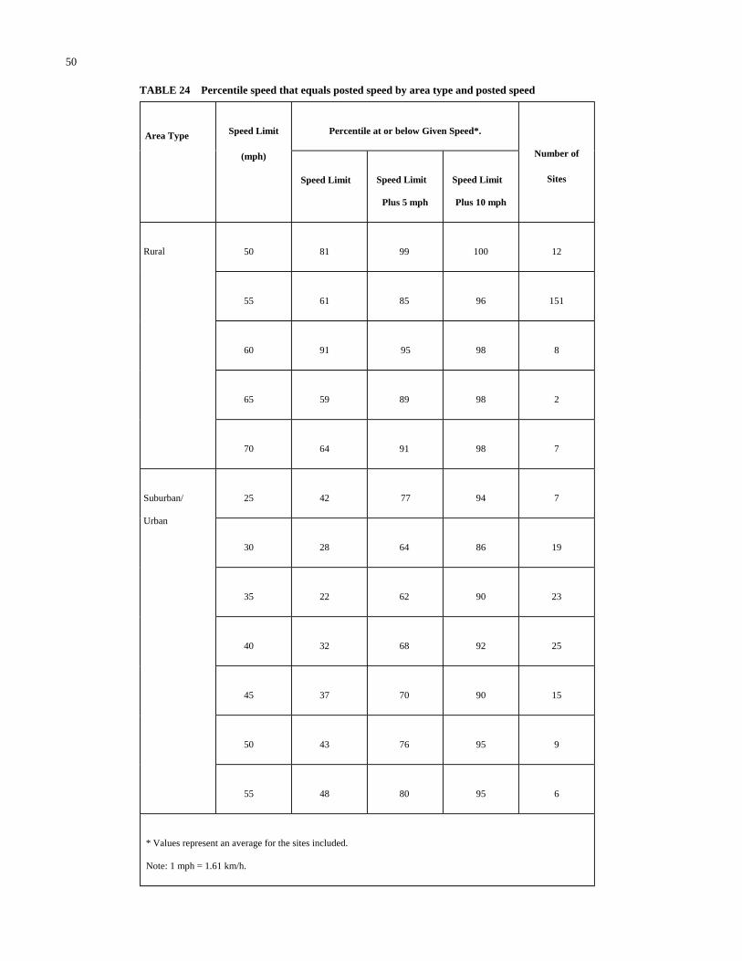
50

TABLE 24 Percentile speed that equals posted speed by area type and posted speed

Percentile at or below Given Speed*.

Area Type

Speed Limit

(mph)

Speed Limit

Speed Limit

Plus 5 mph

Speed Limit

Plus 10 mph

Number of

Sites

50

81

99

100

12

55

61

85

96

151

60

91

95

98

8

65

59

89

98

2

Rural

70

64

91

98

7

25

42

77

94

7

30

28

64

86

19

35

22

62

90

23

Suburban/

Urban

40

32

68

92

25

45

37

70

90

15

50

43

76

95

9

55

48

80

95

6

* Values represent an average for the sites included.

Note: 1 mph = 1.61 km/h.

Procedures Used to Set Speed Limits

The methods used to set speed limits have been reviewedby several authors (22, 54, 55). A recent review was conductedby an Institute of Transportation Engineers (ITE) TechnicalCommittee with the following findings (56).

• The 85th percentile speed is the predominant factor usedin setting speed limits (by 99 percent of the agenciessurveyed). Both roadway geometry and accident expe-riences are “always or usually considered” by more than90 percent of the agencies, and roadside development isalso popular, being considered “always or usually” by85 percent of the respondents.

• In an open-ended question, the top three factors used inestablishing speed zones other than 85th percentilespeed were roadway geometry, accident experience, anda new factor not present in the previous question: politi-cal pressure.

• Most jurisdictions allow deviations from the 85th per-centile speed, with most being between 5 and 10 mph(8.1 and 16.1 km/h). Reasons for the deviation includepolitics (33 percent), accidents (13 percent), roadwayareas (11 percent), and roadway geometry (9 percent).

General guidance on how to set speed limits is provided inseveral locations, such as in the MUTCD (16) and in state orcity manuals. Table 25 summarizes the information provided

51

in the MUTCD (16). A 2001 ITE publication (56) provides asummary of criteria for several states and cities. These doc-uments, however, do not make specific recommendations onhow much to adjust the speed limit when considering schoolchildren, accidents, or the geometrics present.

Operating Speed Compared with New Speed Limits

Figure 6 clearly shows that operating speeds as measured bythe 85th percentile statistic are greater than the posted speedlimit for most roadways. For several conditions, the meanspeed is also in excess of the posted speed limit. In theory, ifspeed limits are set at the 5 mph (8.1 km/h) closest to the 85thpercentile speed, then the posted speed limits should be muchcloser to the 85th percentile operating speeds than shown inTable 24. So a question is “are speed limits set with such dis-parity or do the speeds change after the speed limit is set?” Apart of a survey conducted by the ITE Traffic EngineeringCouncil (TENC) Committee 97-12 was a request for “speedzoning investigations your agency has recently conducted”(56). A total of 256 speed zoning reports were received from124 respondents (average of 2.1 reports per survey). Thematerial contained within the reports varied. For example,some contained only the speed statistics from a computersoftware program with no recommendations on changes tothe existing speed limit. Other reports were complete in-depth

TABLE 25 MUTCD guidelines for speed limits

Standard:

After an engineering study has been made in accordance with established traffic engineering practices, the Speed Limit

(R2-1) sign shall display the limit established by law, ordinance, regulation, or as adopted by the authorized agency.

The speed limits shown shall be in multiples of 10 km/h (5 mph).

Guidance:

When a speed limit is to be posted, it should be the 85th percentile speed of free-flowing traffic, rounded up to the

nearest 10 km/h (5 mph) increment.

Option:

Other factors that may be considered when establishing speed limits are the following:

• Road characteristics, shoulder condition, grade, alignment, and sight distance;

• The pace speed;

• Roadside development and environment;

• Parking practices and pedestrian activity; and

• Reported crash experience for at least a 12-month period.

studies of a roadway’s posted speed limits, including detailson the geometric conditions and accident characteristics ofthe roadway.

Several surveys provided sufficient information to com-pare the 85th percentile speed with the existing and proposedposted speed limits. Plots were generated to illustrate therelationship between the existing posted speed limit and themeasured 85th percentile speed (see Figure 7), the recom-mended posted speed limit and the measured 85th percentilespeed (see Figure 8), and the difference between the mea-sured 85th percentile speed and the recommended speedlimit and the existing speed limit (see Figures 9 and 10).

Figure 7 illustrates findings similar to those collected aspart of this study and presented in Figure 6. In general, for

52

roadways with posted speed limits of 45 mph (72.4 km/h)and below, most of the measured speeds are higher than theposted speed limit. When the posted speed limit is 55 mph(88.5 km/h) or more, only about half of the measured speedsare above the posted speed limit. Figure 8 shows that, inalmost all situations, the recommended posted speed limit isbelow the measured 85th percentile speed. The data weresubdivided by whether the recommendation was for chang-ing a speed limit or maintaining it. Both data sets had simi-lar trends.

An appreciation for the amount of difference between themeasured 85th percentile speed and the recommended postedspeed can be obtained from Figures 9 and 10. Figure 9 showsthat the range of speed differences does not vary by the exist-

0

10

20

30

40

50

60

70

80

0 10 20 30 40 50 60 70 80

Existing Posted Speed Limit (mph)

85th

Per

cen

tile

Sp

eed

(m

ph

)

Figure 7. Existing posted speed limit versus 85th percentile speedfor 128 speed surveys.

0

10

20

30

40

50

60

70

80

0 10 20 30 40 50 60 70 80

Recommended Posted Speed Limit (mph)

85th

Per

cen

tile

Sp

eed

(m

ph

)

Change Posted Speed Limit

Maintain Posted Speed Limit

SL = 85th

Figure 8. Recommended posted speed limit versus 85th percentile speedfor 128 speed surveys.

ing posted speed limit, except at the higher speed limits (55 mph [88.5 km/h] and greater) where the difference is less.Figure 10 shows the cumulative frequency of the difference.About one-half of the sites had between a 4- and 8-mph (6.4-and 12.9-km/h) difference from the measured 85th percentilespeed. At only 10 percent of the sites did the recommendedposted speed limit reflect a rounding up to the nearest 5-mph(8.1-km/h) increment (as stated in the MUTCD, see Table 25).At approximately one-third of the sites, the posted speed limitwas rounded to the nearest 5-mph (8.1-km/h) increment. Forthe remaining two-thirds of the sites, the recommended postedspeed limit was more than 3.6 mph (5.8 km/h) below the 85thpercentile speed.

53

Changes in Posted Speed Limit

A frequently asked question is how much influence doesthe posted speed have on operating speed? If one changes theposted speed, would that change the speeds of the drivers onthe roadway? Both sides of this debate have been argued.Some claim that posted speed limits are irrelevant and haveno impact. Drivers, being reasonable and prudent, will oper-ate their vehicles at a comfortable and safe speed. Operatingspeeds observed on rural two-lane highways during themandatory 55 mph (88.5 km/h) maximum speed limit periodare used as examples. These roads saw speeds in excess of70 mph (112.7 km/h) during this time period, yet had some

0

10

20

30

40

50

60

70

80

-5 0 5 10 15 20 25

Exi

stin

g P

ost

ed S

pee

d L

imit

(m

ph

)

85th Percentile Speed Minus Recommended Posted Speed Limit (mph)

Figure 9. 85th percentile speed minus recommended posted speed limitversus existing posted speed limit for 128 speed surveys.

0

10

20

30

40

50

60

70

80

90

100

-5 0 5 10 15 20

Cu

mu

lati

ve F

req

uen

cy

Difference (85th Percentile Minus Recommended Speed Limit) (mph)

Figure 10. 85th percentile minus recommended posted speed limit versuscumulative frequency for 128 speed surveys.

of the best safety records. Now with the removal of thenational speed limit, these roads are posted with a 70 mph(112.7 km/h) limit. Others comment that drivers are influ-enced by the speed limit, by at least staying within a certainrange to avoid tickets.

Data collected by Parker for an FHWA study included thefollowing findings (53):

• Before the speed limit change, the typical posted speedlimit for the experimental sites was set at the 20th per-centile speed; after the speed limit change, this increasedto the 43rd percentile speed.

• There was generally less than a 2-mph (3.2-km/h) dif-ference in average speeds, speed standard deviation,and 85th percentile speed between the before and afterspeeds. These changes were statistically significant butwere interpreted as “not sufficiently large to be of prac-tical significance.”

• Changes in posted speed limits led to changes in drivercompliance, but this reflects the definition of compli-ance as driving at or below the posted speed limit ratherthan changes in driver behavior.

• Changes in posted speed limits had little effect on high-way safety.

Parker’s work has been referenced to support the argumentthat speed limits do not influence driver’s operating speed.The thought is that because the change in posted speed did notproduce a similar change in operating speed, the posted speeddoes not influence a driver’s speed choice. However, Parker’sstudy had an acknowledged major shortcoming in the siteselection. The sites selected for the speed limit changes werechosen by local agencies on the basis of a predeterminedneed (e.g., request from the public, high incidence of crashes,compliance with local ordinances, changing land use pat-terns) rather than randomly (23). Parker qualified his con-clusions by stating that “the findings may apply to similarsites where the speed limits are changed for similar reasons.Generalization to other roadways are not appropriate.” There-fore, the question still remains on how much influence aposted speed has on operating speed.

DISTRIBUTIONS OF CHARACTERISTICS

Ranges for design elements can vary from one region toanother or from one city to another. Identifying these poten-tial variations can help engineers to gain a more complete pic-ture of the variables that are involved in specifying values fordesign elements. An approach to design that uses establishedroadway classes needs to provide information on acceptableranges within each design element. Going beyond that range,such as having curb and gutter rather than shoulders, cancommunicate a different roadway environment to the driverand result in a different speed distribution for the road as

54

compared with the same type of road in a different area of thecountry. A new approach will not be accepted if it recom-mends major changes to the roadway network, especially ifthose recommendations cannot be supported with strong evi-dence that the changes will result in a noticeable improve-ment in safety or speed consistency.

Data Collection and Reduction

Roadway and roadside characteristics data for a sample ofroadways within three cities and three predominantly ruralcounties were collected. The roadways were to include exam-ples of flat, rolling, and mountainous terrain. The researchteam reviewed the following to aid in creating a short list ofcandidate areas:

• population of cities, • terrain present, • contacts who could aid in gathering maps or other

needed information, • potential overlap with data collection efforts for the field

speed studies, and • reasonable data collection routes.

Based on the above, the following areas were selected:

Cities (2000 population) Counties

College Station, TX (60,000) Brazos County, TXPortland, OR (486,000) Somerset County, PALittle Rock, AR (175,000) Skagit County, WA

College Station, Texas

A database of streets in College Station was created usinga city map. Data were collected by driving approximately200 street segments and recording measurements while in thefield. Collected data included information such as number ofdriveways, intersections, and signals; vertical profile; road-side environment; speed limit; roadside hazard; shoulder typeand width; median type and width; lane width; and presenceof on-street parking, bike lanes, or sidewalks. The city mapwas used to count the number of horizontal curves, calculatethe average deflection angles, and obtain precise lengths foreach street. In College Station, almost all of the local, col-lector, and arterial (intermediate and suburban) streets havecurb and gutter (between 78 and 95 percent). Only 13 percentof the high-speed arterial streets had curb and gutter, with theremainder having shoulders. The average lane width washigher for the lower functional classes (local, collectors, andintermediate arterials) than the suburban or high-speed arte-rials. Only 21 percent of the local streets had sidewalks;however, 70 percent of the collectors and about one-half of

the arterials had sidewalks. Driveway density decreased asthe functional classification increased. Local streets had aweighted average of 78.7 driveways/mi (48.9 driveways/km),which equates to a spacing of approximately 67 ft (20.4 m)between driveways. Collectors and suburban arterials haveweighted averages of 20.2 and 14.3 driveways/mi (12.6 and8.9 driveways/km), respectively, which correspond to 261and 370 ft (79.6 and 112.8 m) between driveways. The typeof development for collectors and locals was uniformly res-idential; however, the other functional classes showed morevariety (residential, commercial, park, etc.), which can con-tribute to the greater variety in posted and operating speedsalong those corridors.

Little Rock, Arkansas

Using a detailed city map, a database was created that con-tains the name of each street within the city limits of LittleRock in the area south of Interstate 630 and west of U.S.Highway 65. Portions of selected neighborhoods in this areawere driven and videotaped to record data for a sample of thestreets on the street network. Collected data included numberof driveways, intersections, and signals; vertical profile; road-side environment; speed limit; roadside hazard; shoulder typeand width; median type and width; lane width; and presenceof on-street parking, bike lanes, or sidewalks. About three-fourths of the collectors and locals in Little Rock have curband gutter, with only 28 and 16 percent, respectively, hav-ing sidewalks. All the suburban arterial mileage has curband gutter and four lanes, with 75 percent also having side-walks. Driveway density in Little Rock is greater than thatfound in College Station. Local streets had 75.8 driveways/mi (47.1 driveways/km), which represents a 70-ft (21.3-m)spacing. Collectors, suburban arterials, and high-speed arte-rials had similar driveway densities, ranging from 35.5 to29.7 driveways/mi (22.1 to 18.5 driveways/km), which equatesto a spacing of 150 ft (45.7 m) for collectors and suburbanarterials and 178 ft (54.3 m) for high-speed arterials. CollegeStation’s high-speed arterials had a 1,148-ft (349.9-m) drive-way spacing.

Portland, Oregon

Portland is unique in that it has a database that includesnearly every street in four counties. The base network mostclosely resembles conditions in 1997. A copy of the Metro’sall-street network used for planning was provided for use inthis project. The fields include segment length, street name,street classification, direction type (one-way or two-way),county, city, speed limit, functional class, number of lanes,and other fields. Each segment’s length (or link) includes astreet name, left- and right-side address, and a from-node IDand to-node ID, which were based on unique nodes at each

55

X, Y, Z location. To be able to identify where a specific linkis on a map, cross street names are needed. If this informa-tion is available, then the number of intersections and thenumber of signalized intersections could be counted from themap or the number of driveways counted in the field couldbe associated with a specific section of roadway. Unfortu-nately, several efforts to obtain the names of the cross streetsassociated with the node numbers were not successful, thuslimiting the ability to expand the roadway segment charac-teristics available.

The number of miles of roadway by functional class andspeed limit were pulled from the database. In each case themajority of miles for a functional class represented a postedspeed limit that would be expected for the class. There weresome examples where the functional classes did include road-way segments with speed limits that do not agree with theexpectations for the class. For example, the local street func-tional class included a few segments with posted speeds typ-ically associated with higher functional classes of roadways.The majority of miles were at 25 mph (40.2 km/h) (192 mi[309.0 km]) with a few at 30 mph (48.3 km/h) (14 mi [22.5 km/h]) and 35 mph (56.3 km/h) (27 mi [43.5 km]);however, several miles were at 45 mph (72.4 km/h) (13 mi[20.9 km]) and 50 mph (80.5 km/h) (9 mi [14.5 km]). Hav-ing a “local” street with a 45- or 50-mph (72.4- or 80.5-km/h)speed limit provides an inconsistent message to the driver.These inconsistencies are easier to identify when databaseson the order of the one being used in Portland are available.The questionable speed limits may be a function of a mis-coded functional class rather than an incorrect speed limit.

Brazos County, Texas

The network of roads considered for Brazos County, Texas,included all U.S., state, and county roads not located withincity limits. The database of the U.S. and state roads wasobtained from TxDOT and included highway number, length,class, shoulder type, and ADT (Average Daily Traffic) range.

To collect additional data for the project, such as numberof driveways, the entire length of each U.S. and state ruralroad was driven and videotaped. Data collected with a dis-tance measuring instrument and software developed at TTIincluded number of driveways, intersections, and signals.Characteristics were also obtained for roads not on the statesystem (i.e., county roads) using the detailed county map. Thelowest posted speed limit for each of the rural roadways was55 mph (88.5 km/h) with shoulder widths ranging between 0and 12 ft (0 and 3.6 m). Lane widths were almost always 12 ft(3.6 m). Driveway density and intersection density were about10 access points per mi (6.2 access points per km) with no clearrelationship of density to functional class (one could expecthigher densities for the lower functional classes). The roundedaverage access point spacing was about 500 ft (152.4 m).

Skagit County, Washington

Based on advice from representatives within the Wash-ington State Department of Transportation, Skagit Countywas selected to represent a rural, mountainous county. Anelectronic copy of the 2000 State Highway Log was obtainedand used to construct the beginning of the database. Wash-ington State maintains videologs of their roads on a website. This web site was used and the roads “driven” to countnumber of driveways and intersections and to gather otherinformation such as roadside environment. The lower roadclasses had lower speeds. Major collectors had posted speedsbetween 25 and 55 mph (40.2 and 88.5 km/h), while the free-ways had posted speeds between 60 and 70 mph (96.6 and112.7 km/h). Shoulder widths also increased as the func-tional class increased. Weighted average shoulder width formajor collectors was 3.4 ft (1.0 m), for minor arterials it was5.7 ft (1.7 m), for principal arterials it was 6.4 ft (2.0 m), andfor freeways it was 10 ft (3.0 m). Lane width followed a sim-ilar pattern, widening from 10.7 ft (3.3 m) (major collector)to 13.4 ft (4.1 m) (freeway). The major collectors had higherdriveway and access point densities than the arterials. Themajor collector had a typical rounded access point spacing of400 ft (121.9 m), while the arterials had a spacing of about800 ft (243.8 m).

Somerset County, Pennsylvania

The Pennsylvania Department of Transportation providedan electronic database of the state-maintained roads withinSomerset County. With the extensive number of state andcounty roads on the Somerset County network, it was decidedto concentrate efforts on the northern portion of the county,specifically that portion north of Interstate 70/76. A sampleof roadways was driven and videotaped. The video tapeswere reviewed in the office, and data on driveway and inter-section density were reduced. For the roads driven in Penn-sylvania, the lower functional classes had narrower shouldersand lanes. Major collector typical shoulder width was 1.9 ft(0.6 m) while minor arterials had 3.2 ft (1.0 m), and freewayshad 8.3 ft (2.5 m). The driveway densities for the Pennsyl-vania sites were unexpected. The lower functional class (minorcollector) only had 5.8 driveways per mile (3.6 driveways perkilometer), while the higher functional classes (minor arter-ial and major collector) had between 11.3 and 14.7 drivewaysper mile (7.0 and 9.1 driveways per kilometer) (weightedaverage). The low value for minor collectors may be a func-tion of the limited sample size for the functional class (only4.9 mi [7.9 km] were driven).

Distribution of Rural Roadway Characteristics

For roads driven in all three counties, there are some note-worthy observations that can be made from the characteris-

56

tics collected. Roads in Brazos County had a fairly constantrange of posted speeds (55 to 70 mph [88.5 to 112.7 km/h]) andoperating speeds (55 to 75 mph [88.5 to 120.7 km/h]), whileroads in Skagit County had a wider variety of posted speedsthat increased as the roadway design class progressed frommajor collector to freeway. In general, the ADT increased asthe design class increased, with the exception of freeways inSomerset County. Average lane widths were between 9.4 and13.4 ft (2.9 and 4.1 m) for all categories; Brazos and SkagitCounties were very consistent in lane widths across all classes,and average lane widths tended to increase as the importanceof the design class increased. Presence and width of shoul-ders was inconsistent in all three counties; widths rangedfrom 0 to 12 ft (0 to 3.6 m), with averages from 0 to 11.2 ft(0 to 3.4 m). However, the average shoulder width increasedas the design class progressed from collector to freeway.

The use of wide medians on freeways was similarly dis-tributed among all three counties, but median widths on otherclasses were widely scattered. In general, arterials had smallermedians and collectors had little to no median width. Drive-way densities were also scattered among the design classes;freeways consistently had little to no driveway presence,while arterials and collectors had a significant presence. Ramp/intersection densities followed a trend similar to drivewaydensities. The access point spacing on the major collectorsand minor arterials in Pennsylvania (about 400 ft [121.9 m]between driveways/intersections) is closer than found in othercounties (approximately 800 ft [243.8 m] in Washington and600 ft [182.9 m] in Texas).

Distribution of S/U Roadway Characteristics

The evaluation of S/U characteristics included considera-tion of the urban and suburban sites available from the fieldspeed data (see Appendix E). The cities included in the eval-uation (and their 2000 populations) are as follows:

Roadway Inventory Cities

College Station, TX (68,000)Little Rock, AR (183,000)

Field Speed Data Cities

Boston, MA (589,000)College Station, TX (68,000)Houston, TX (1,954,000)Little Rock, AR (183,000)Nashville, TN (546,000)Portland, OR (529,000)St. Louis, MO (348,000)

The data were categorized as being from College Station,Little Rock, or field data. For the field data category, the

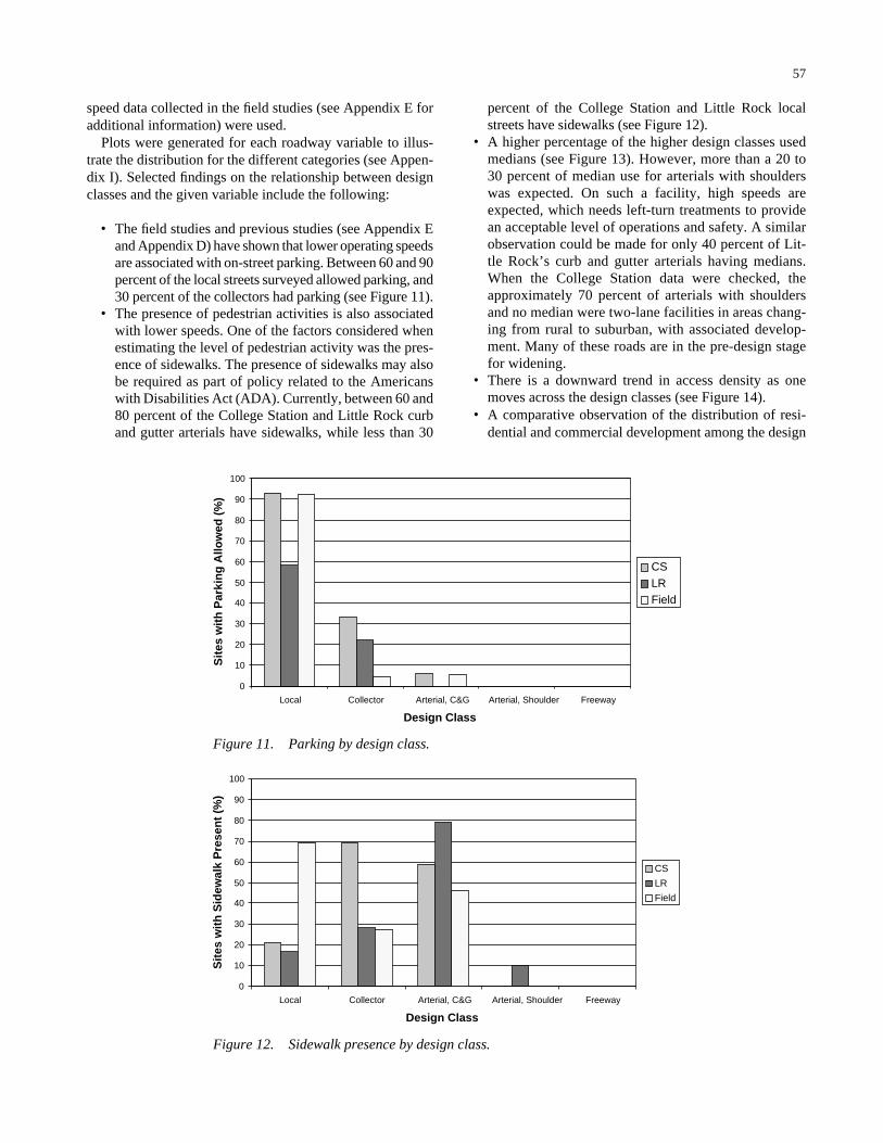
speed data collected in the field studies (see Appendix E foradditional information) were used.

Plots were generated for each roadway variable to illus-trate the distribution for the different categories (see Appen-dix I). Selected findings on the relationship between designclasses and the given variable include the following:

• The field studies and previous studies (see Appendix Eand Appendix D) have shown that lower operating speedsare associated with on-street parking. Between 60 and 90percent of the local streets surveyed allowed parking, and30 percent of the collectors had parking (see Figure 11).

• The presence of pedestrian activities is also associatedwith lower speeds. One of the factors considered whenestimating the level of pedestrian activity was the pres-ence of sidewalks. The presence of sidewalks may alsobe required as part of policy related to the Americanswith Disabilities Act (ADA). Currently, between 60 and80 percent of the College Station and Little Rock curband gutter arterials have sidewalks, while less than 30

57

percent of the College Station and Little Rock localstreets have sidewalks (see Figure 12).

• A higher percentage of the higher design classes usedmedians (see Figure 13). However, more than a 20 to30 percent of median use for arterials with shoulderswas expected. On such a facility, high speeds areexpected, which needs left-turn treatments to providean acceptable level of operations and safety. A similarobservation could be made for only 40 percent of Lit-tle Rock’s curb and gutter arterials having medians.When the College Station data were checked, theapproximately 70 percent of arterials with shouldersand no median were two-lane facilities in areas chang-ing from rural to suburban, with associated develop-ment. Many of these roads are in the pre-design stagefor widening.

• There is a downward trend in access density as onemoves across the design classes (see Figure 14).

• A comparative observation of the distribution of resi-dential and commercial development among the design

0

10

20

30

40

50

60

70

80

90

100

Local Collector Arterial, C&G Arterial, Shoulder Freeway

Design Class

Sit

es w

ith

Par

kin

g A

llow

ed (

%)

CSLRField

Figure 11. Parking by design class.

0

10

20

30

40

50

60

70

80

90

100


Design Class

Sit

es w

ith

Sid

ewal

k P

rese

nt

(%)

CS

LR

Field

Figure 12. Sidewalk presence by design class.

classes shows that the percentage of arterials with curband gutter that have residential development is nearlyidentical to the percentage that have commercial devel-opment. The mixed use of development could helpexplain the wide range of speeds recorded on arterialswith curb and gutter.

Key findings from the comparison of a roadway elementwith posted speed include the following:

• A high percent of the lower posted speed roadways hadon-street parking, as expected (see Figure 15).

• The use of sidewalks does not appear to be stronglyrelated to the posted speed of the facility in the two cities(see Figure 16).

• Driveway density has the expected relationship withthe speed ranges—the number of driveways per miledecreases as the speed range increases (see Figure 17).

58

• College Station, Little Rock, and the field speed datafollowed similar trends with respect to the percent ofsites with residential or commercial development (seeFigures 18 and 19). Lower posted speed limit sites hadmore residential development, while higher posted speedlimit sites had more commercial development.

ROADWAY DESIGN CLASS APPROACH

Background

Geometric design refers to the selection of roadway ele-ments that include the horizontal alignment, vertical align-ment, cross section, and roadside of a highway or street. Ingeneral terms, good geometric design means providing theappropriate level of mobility and land use access for motorists,bicyclists, and pedestrians while maintaining a high degreeof safety. The roadway design must also be cost effective intoday’s fiscally constrained environment. While balancing

0

10

20

30

40

50

60

70

80

90

100


Design Class

Sit

es w

ith

Med

ian

(%

)CSLRField

Figure 13. Median presence by design class.

0

20

40

60

80

100

120


Design Class

Acc

ess

Den

sity

(p

ts/m

i)

CS

LR

Field

Figure 14. Access density by design class.

these design decisions, the designer needs to provide consis-tency along a roadway to prevent abrupt changes in thedesign that do not match motorists’ expectations. In addition,the designer needs to select appropriate values for the differ-ent roadway variables to communicate to the driver the appro-priate speed and operations along a facility. Providing sev-eral lanes, a straight and relatively level alignment, few access

59

points, and an open roadside environment will not encouragedrivers to maintain low speeds. To increase the designer’sappreciation that the overall look of a roadway will influencethe operations along a facility, the roadway design classapproach has been developed.

The classification of roadways into different operationalsystems, functional classes, or geometric types is necessary for

0

10

20

30

40

50

60

70

80

90

20-30 25-35 30-40 35-45 40-50 45-55 50-60 55-65 60-70

Posted Speed Range (mph)

Sit

es w

ith

Par

kin

g A

llow

ed (

%)

CS

LR

Field

Figure 15. Parking by posted speed range.

0

10

20

30

40

50

60

70

80

90

100

20-30 25-35 30-40 35-45 40-50 45-55 50-60 55-65 60-70


Sit

es w

ith

Sid

ewal

ks (

%)

CS

LR

Field

Figure 16. Sidewalks by posted speed range.

communication among engineers, administrators, and the gen-eral public. Various classification schemes have been appliedfor different purposes for rural and urban regions. The mostcommon scheme used within the roadway design and trafficoperations groups is functional classification, which includesthree major divisions: arterial, collector, and local. This clas-sification scheme emphasizes the type of service or function

60

the roadway is to provide. The determination is made basedupon whether the roadway is primarily for access (i.e., localstreet), for mobility (i.e., arterials), or a mix (i.e., collectors).The classification scheme does not provide the level of detailneeded to establish unique characteristics between road-ways that provide similar functions but at different levels. Forexample, an interstate freeway and a four-lane high-speed

0

10

20

30

40

50

60

70

20-30 25-35 30-40 35-45 40-50 45-55 50-60 55-65 60-70


Dri

vew

ay D

ensi

ty (

drv

/mi)

CS

LR

Field

Figure 17. Driveway density by posted speed range.

0

10

20

30

40

50

60

70

80

90

100

20-30 25-35 30-40 35-45 40-50 45-55 50-60 55-65 60-70


Sit

es w

ith

Res

iden

tial

Dev

elo

pm

ent

(%)

CS

LR

Field

Figure 18. Residential development by posted speed range.

arterial provide the same function (mobility) but have verydifferent design qualities. The freeway would provide accessby ramps and would not have signals, while the four-lane high-speed arterial would have some driveways, some provision forleft turns across opposing traffic streams, and signals. To bet-ter align design criteria with a classification scheme, a road-way design class was created. To recognize some of the sim-ilarities between the classes for the roadway design classscheme and the functional classification scheme, similar titleswere used.

Development

The process for developing a roadway design class approachbegan with identifying roadway and roadside characteristicsthat could be logically grouped to describe a type of road.Information from the mailout surveys (see Appendix B), theliterature (see Appendix D), and existing reference materials(e.g., Green Book) were used to determine preliminary groups.Grouping freeway and local street characteristics was simple.Determining the splits for roads between those limits was notas simple. The goal of the field studies was to identify the char-acteristics that, as a group, would produce a distinct speed. Forexample, what are the characteristics that would result in ahigh speed and high mobility performance as opposed to thosecharacteristics that would result in a lower speed. The resultsof the field studies (see Appendix E) demonstrated that theinfluences on speed are complex. Even when features that areclearly associated with a local street design are present (e.g.,no pavement markings, on-street parking, two lanes, etc.), 85th

61

percentile speeds still ranged between 26 and 42 mph (41.8and 67.6 km/h) for the 13 sites. Such wide ranges of speeds arealso present for other groupings of characteristics.

Adding to the complexity is the variation in features thatare currently present for different roadway groups. Becauseof the rigid design features associated with freeways, freewaysare easy to identify. When access is controlled by ramps andeither a wide median or a barrier separates opposing traffic,then the roadway is probably a freeway. The distribution ofexisting features associated with other streets is not so clear.As shown in Appendix I, certain features are related to theclasses. For example, the number of lanes increases and theuse of on-street parking decreases as the class of roadwaygoes from local to freeway. The relationships for other fea-tures are not so clear. Is a characteristic of local or collectorstreets the provisions for pedestrians? If so, then a high per-centage of those facilities should have sidewalks. However,for the two cities surveyed, only 20 and 18 percent of thelocal streets and 70 and 27 percent of the collectors had side-walks. If the recommendation in a roadway design classapproach is that all local or collector streets have sidewalks(to provide for consistency for this road type between citiesand states), then several existing facilities would not meet theguidelines.

Because of the variability in speeds observed in the fieldfor the different roadway classes and the large distribution inexisting roadway characteristics, the splits between differentroadway design classes need to be determined using a com-bination of engineering judgment and policy decisions. Fol-lowing is the research team recommendation for roadwaydesign classes.

0

10

20

30

40

50

60

70

80

90

100

20-30 25-35 30-40 35-45 40-50 45-55 50-60 55-65 60-70


Sit

es w

ith

Co

mm

erci

al D

evel

op

men

t (%

)

CS

LR

Field

Figure 19. Commercial development by posted speed range.

Roadway Design Classification Procedure

A decision tree of the roadway design classification proce-dure is shown in Figure 20. The completion of the first threesteps leads to the appropriate roadway design class. Tables 26and 27 provide an overview of the different classes within theS/U and rural environments, respectively. These tables can beused to assist in selecting the appropriate class.

Features identified as being related to operating speedinclude (in general order of the strength of the relationship)posted speed limit, functional classification, access density,median presence, and on-street parking. Other features thathave been shown to be related to the speed level include pedes-trian activity, use of pavement markings, distance betweenfeatures that are known to control speed (e.g., signals), andthe signal density. The value selected for these features or thepresence of the feature should be considered in the design ofa facility.

The appropriate roadway design class can be determinedusing the flow chart in Figure 20 or by reviewing the charac-teristics tables (see Tables 26 and 27). Example pictures,along with a brief description for each roadway design class,are provided in Tables 28 through 37. This information canbe used to verify that the selected roadway design class fitsthe designer’s intentions.

The following steps are used within the roadway designclassification procedure:

Step 1: Decide if the facility will be in a rural or S/Uarea.

According to the Green Book, urban and rural areas havefundamentally different characteristics with regard to den-

62

sity and types of lane use, density of street and highwaynetworks, nature of travel patterns, and the way in whichthese elements are related. Urban areas are considered tobe those places within boundaries set by the responsiblestate and local officials having a population of 5,000 ormore. Urban areas are further subdivided into urbanizedareas (population of 50,000 and over) and small urbanareas (population between 5,000 and 50,000). For designpurposes, the population forecast for the design yearshould be used. Rural areas are those areas outside theboundaries of urban areas. For the roadway design class,suburban/urban areas should be considered the traditionalurban areas as defined in the Green Book.

Step 2: Determine the type of service to be provided bythe facility.

The Green Book explains that roadway networks providedual roles in that they provide both access to property andtravel mobility. Regulated access control is needed onarterials to ensure their primary function of mobility. Onthe other hand, the function of local roads and streets is toprovide access, which inherently limits mobility. The rela-tionship between mobility and access is one of give andtake, with collectors and arterials serving both purposes.

Step 3: Select the anticipated operating speed or adjustedposted speed.

Once the environment and type of service have beenselected, the next step is to estimate the speed at which thefacility is to operate once completed. This speed can be the

Suburban/Urban

55 to 70

Roadway Design ClassEnvironment Service

Anticipated Operating Speed

(or Adjusted PostedSpeed), (mph)

Rural

55 or higher

35 to 70

45 to 70

30 or less

45 to 55

55 or higher

30 to 40

30 to 45

30 or less

Mixed

Access

Principal Arterial

Freeway

Collector

Minor Arterial

Local

Freeway

Collector

Mobility

Mixed

Access

Mobility

Local

Principal Arterial

Major Arterial

Figure 20. Roadway design class flow chart.

(text continues on page 78)

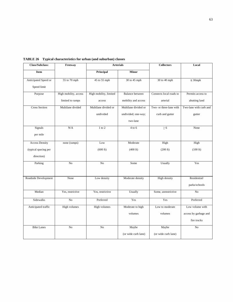
63

TABLE 26 Typical characteristics for urban (and suburban) classes

Class/Subclass: Freeway Arterials Collectors Local

Item Principal Minor

Anticipated Speed or

Speed limit

55 to 70 mph 45 to 55 mph 30 to 45 mph 30 to 40 mph ≤ 30mph

Purpose High mobility, access

limited to ramps

High mobility, limited

access

Balance between

mobility and access

Connects local roads to

arterial

Permits access to

abutting land

Cross Section Multilane divided Multilane divided or

undivided

Multilane divided or

undivided; one-way;

two-lane

Two- or three-lane with

curb and gutter

Two-lane with curb and

gutter

Signals

per mile

N/A 1 to 2

4 to 6

> 6

None

Access Density

(typical spacing per

direction)

none (ramps) Low

(600 ft)

Moderate

(400 ft)

High

(200 ft)

High

(100 ft)

Parking

No No Some Usually Yes

Roadside Development None Low density Moderate density High density Residential/

parks/schools

Median Yes, restrictive Yes, restrictive Usually Some, unrestrictive No

Sidewalks No Preferred Yes Yes Preferred

Anticipated traffic High volumes High volumes Moderate to high

volumes

Low to moderate

volumes

Low volume with

access by garbage and

fire trucks

Bike Lanes No No Maybe

(or wide curb lane)

Maybe

(or wide curb lane)

No

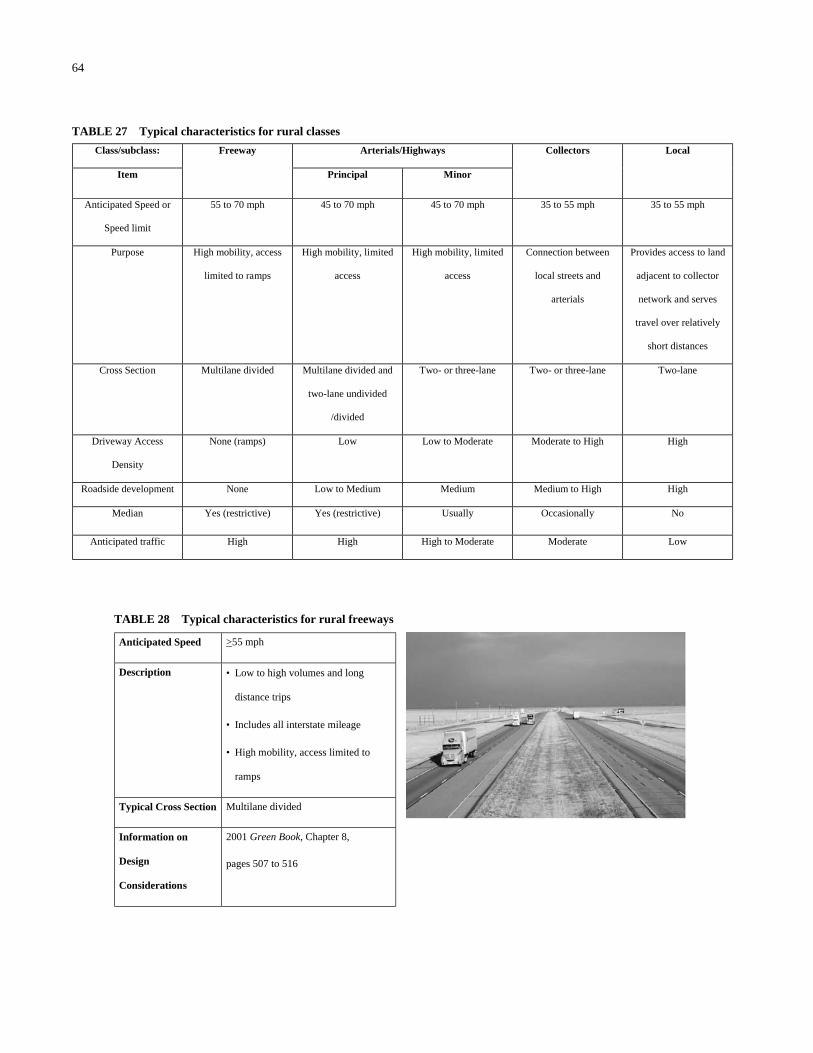
64

TABLE 27 Typical characteristics for rural classes

Class/subclass: Freeway Arterials/Highways Collectors Local

Item Principal Minor


Speed limit

55 to 70 mph 45 to 70 mph 45 to 70 mph 35 to 55 mph 35 to 55 mph

Purpose High mobility, access

limited to ramps


access


access

Connection between

local streets and

arterials

Provides access to land

adjacent to collector

network and serves

travel over relatively

short distances

Cross Section Multilane divided Multilane divided and

two-lane undivided

/divided

Two- or three-lane Two- or three-lane Two-lane

Driveway Access

Density

None (ramps) Low Low to Moderate Moderate to High High

Roadside development None Low to Medium Medium Medium to High High

Median Yes (restrictive) Yes (restrictive) Usually Occasionally No

Anticipated traffic High High High to Moderate Moderate Low

TABLE 28 Typical characteristics for rural freeways

Anticipated Speed >55 mph

Description • Low to high volumes and long

distance trips

• Includes all interstate mileage

• High mobility, access limited to

ramps

Typical Cross Section Multilane divided

Information on

Design

Considerations

2001 Green Book, Chapter 8,

pages 507 to 516

65

TABLE 29 Typical characteristics for rural principal arterials

Anticipated Speed >45 mph

Description • High volumes and long distance

trips

• Provide for relatively high travel

speeds and minimum interference to

through movement

• High mobility, limited access

Typical Cross Section Multilane divided and undivided

Information on

Design

Considerations


pages 507 to 516

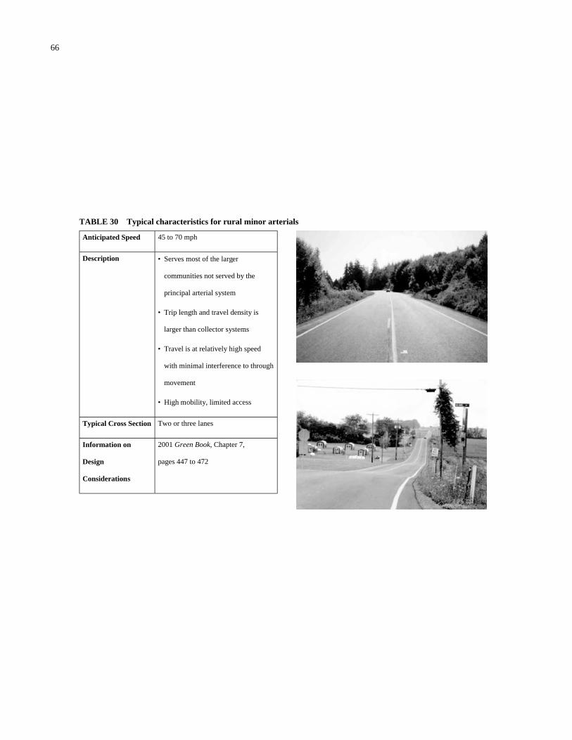
66

TABLE 30 Typical characteristics for rural minor arterials

Anticipated Speed 45 to 70 mph

Description • Serves most of the larger

communities not served by the

principal arterial system

• Trip length and travel density is

larger than collector systems

• Travel is at relatively high speed

with minimal interference to through

movement

• High mobility, limited access

Typical Cross Section Two or three lanes

Information on

Design

Considerations


pages 447 to 472

67

TABLE 31 Typical characteristics for rural collectors


Description • Travel is of intra county and

regional importance rather than

statewide importance.

• Roads provide service to any county

seat not on an arterial road.

• Connection between local streets

and arterials.

Typical Cross Section Two lanes

Information on

Design

Considerations


pages 507 to 516

68

TABLE 32 Typical characteristics for rural local streets


Description • Roads to residential development or

to isolated industry facility.

• Feeds traffic to collectors.

• Access to abutting land.

Typical Cross Section Two lanes

Information on

Design

Considerations


pages 383 to 393

69

TABLE 33 Typical characteristics for suburban/urban freeways

Anticipated Speed

≤ 55mph

Description

High mobility, access limited to ramps

Typical Cross Section

Multilane divided

Information on Design

Considerations


pages 507 to 512 and 517 to

558

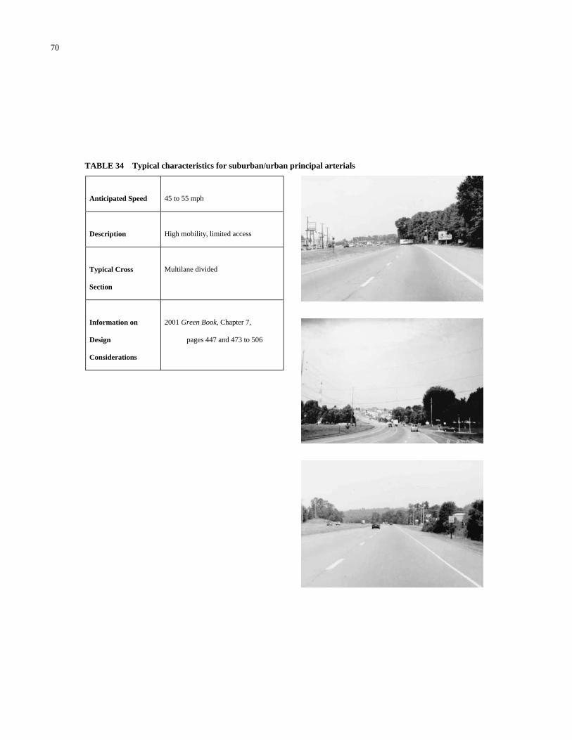
70

TABLE 34 Typical characteristics for suburban/urban principal arterials

Anticipated Speed

45 to 55 mph

Description

High mobility, limited access

Typical Cross

Section

Multilane divided

Information on

Design

Considerations


pages 447 and 473 to 506

71

TABLE 35 Typical characteristics for suburban/urban minor arterials

Anticipated Speed

35 to 55 mph

Service

Balance between mobility and access

Typical Cross

Section

Multilane divided or undivided; one

way; two lane

In CBD could be one way; two way,

two or more lanes

Information on

Design

Considerations



72

TABLE 36 Typical characteristics for suburban/urban collectors

Anticipated Speed

30 to 50 mph

Service

Connects local roads to arterial

Typical Cross

Section

Two or three lanes with curb and

gutter

Information on

Design

Considerations


pages 423 to 424 and 433 to 445

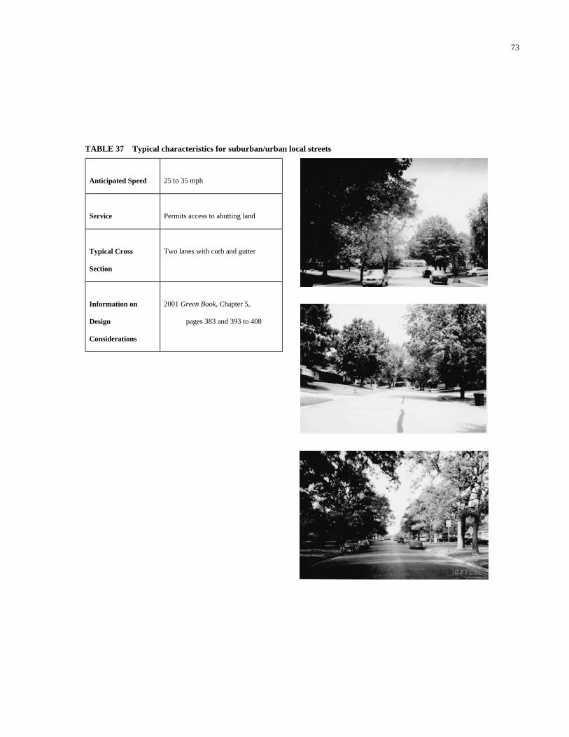
73

TABLE 37 Typical characteristics for suburban/urban local streets

Anticipated Speed

25 to 35 mph

Service

Permits access to abutting land

Typical Cross

Section

Two lanes with curb and gutter

Information on

Design

Considerations



74

Cycle Length (seconds)

50 60 70 80 90 100

Source: Transportation and Land Development, ITE, 1998

20

30

40

50

60

Spe

ed (

mph

)

Off-Peak

Peak

Figure 21. Operating speed depending on anticipatedsignal spacing and cycle length.

TABLE 38 Regression equations for calculating estimated 85th percentilespeed

The data from the field studies produced the following regression equation for predicting operating speed using posted speed limit:

All roadways (Ro2 = 0.904)

EV85 = 7.675 + 0.98 (PSL)

Where:

EV85 = Estimated 85th percentile speed (mph) PSL = posted speed limit (mph)

If the functional class of the roadway is known, the following regression equations can be used for predicting operating speed using posted speed limit:

Suburban/Urban Arterial (Ro2 = 0.86)

EV85 = 8.666 + 0.963 (PSL)

Suburban/Urban Collector (Ro

2 = 0.41)

EV85 = 21.131 + 0.639 (PSL)

Suburban/Urban Local (Ro2 = 0.14)

EV85 = 10.315 + 0.776 (PSL)

Rural Arterial (Ro

2 = 0.81)

EV85 = 36.453 + 0.517 (PSL)

TABLE 39 Typical dimensions for urban (and suburban) classes

Class/Subclass:

Arterials

Item

Freeway

Principal

(Nonfreeway)

Minor

Collectors

Local


Speed limit (mph)

55 to 70

45 to 55

30 to 45

35 to 45

≤ 30

CROSS SECTION

Lane Width (ft)

12

11 to 12

10 to 12

10 to 12

industrial: 12

residential: 9 to 11

industrial: 11 to 12

Shoulder Width (ft)

Right = 10

Left = 4 to 8

8 to 10

Parking lanes not

recommended

8 (if used), or

10 to 12 (parking lane)

2 to 6 (if used), or

7 to 8 (parking lane)

2 (if used), or

7 (parking lane)

Clear Zone (ft)

30

Curbed = 1.5,

otherwise 10

Curbed = 1.5,

otherwise 10

Curbed = 1.5,

otherwise 10

Curbed = 1.5,

otherwise 7 to 10

Median Width (ft)

Lanes Min Width

4 10

6 22 - 26

12 to 18

TWLTL = 12 to 18

TWLTL = 10 to 16

N/A

ALIGNMENT

Radius (minimum)

See tables in Green Book (17)

See tables in Green Book (17)


12

8 with snow & ice

Avoid

but max = 6

Avoid

but max = 6

Avoid

but max = 4

Maximum

Grade (%)

3 to 4 (level)

4 to 5 (rolling)

5 to 8 (level)

6 to 9 (rolling)

up to 8, desirably less

than 5

5 to 9 (level)

6 to 12 (rolling)

up to 15

Cross Slope (%) 1.5 to 2.0 1.5 to 3.0 1.5 to 3.0 1.5 to 3.0 0.5 to 1.0

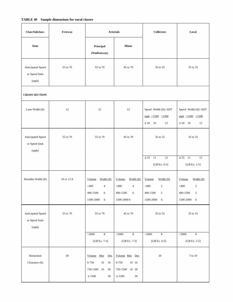
TABLE 40 Sample dimensions for rural classes

Class/Subclass:

Arterials

Item

Freeway

Principal

(Nonfreeway)

Minor

Collectors

Local

Anticipated Speed

or Speed limit

(mph)

55 to 70

55 to 70

45 to 70

35 to 55

35 to 55

CROSS SECTION

Lane Width (ft)

12

12

12

Speed Width (ft)/ ADT

mph <1500 >1500

≤ 50 10 12

Speed Width (ft)/ ADT

mph <1500 >1500

≤ 50 10 12

Anticipated Speed

or Speed limit

(mph)

55 to 70

55 to 70

45 to 70

35 to 55

35 to 55

≥ 55 11 12

[GB Ex. 6-5]

≥ 55 11 12

[GB Ex. 5-5]

Shoulder Width (ft)

10 to 12 ft

Volume Width (ft)

<400 4

400-1500 6

1500-2000 6

Volume Width (ft)

<400 4

400-1500 6

1500-2000 6

Volume Width (ft)

<400 2

400-1500 5

1500-2000 6

Volume Width (ft)

<400 2

400-1500 5

1500-2000 6

Anticipated Speed

or Speed limit

(mph)

55 to 70 55 to 70 45 to 70 35 to 55 35 to 55

>2000 8

[GB Ex. 7-3]

>2000 8

[GB Ex. 7-3]

>2000 8

[GB Ex. 6-5]

>2000 8

[GB Ex. 5-5]

Horizontal

Clearance (ft)

30

Volume Min Des

0-750 10 16

750-1500 16 30

≥ 1500 30

Volume Min Des

0-750 10 16

750-1500 16 30

≥ 1500 30

10

7 to 10

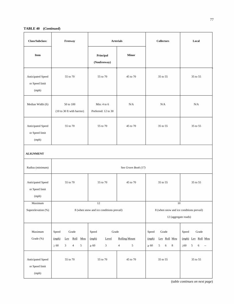
77


Class/Subclass:

Arterials

Item

Freeway

Principal

(Nonfreeway)

Minor

Collectors

Local

Anticipated Speed

or Speed limit

(mph)

55 to 70

55 to 70

45 to 70

35 to 55

35 to 55

Median Width (ft)

50 to 100

(10 to 30 ft with barrier)

Min: 4 to 6

Preferred: 12 to 30

N/A

N/A

N/A

Anticipated Speed

or Speed limit

(mph)

55 to 70 55 to 70 45 to 70 35 to 55 35 to 55

ALIGNMENT

Radius (minimum)

See Green Book (17)

Anticipated Speed

or Speed limit

(mph)

55 to 70 55 to 70 45 to 70 35 to 55 35 to 55

Maximum

Superelevation (%)

12

8 (when snow and ice conditions prevail)

10

8 (when snow and ice conditions prevail)

12 (aggregate roads)

Maximum

Grade (%)

Speed Grade

(mph) Lev Roll Mou

> 60 3 4 5

Speed Grade

(mph) Level Rolling Mount

≥ 60 3 4 5

Speed Grade

(mph) Lev Roll Mou

≥ 60 5 6 8

Speed Grade

(mph) Lev Roll Mou

>60 5 6 --

Anticipated Speed

or Speed limit

(mph)

55 to 70 55 to 70 45 to 70 35 to 55 35 to 55

(table continues on next page)

anticipated operating speed, the posted speed, the antici-pated posted speed plus a set increment such as 5 or 10 mph(8.1 or 16.1 km/h), or the adjusted operating speed asdetermined using a regression equation and then roundedto nearest 5 mph (8.1 km/h).

It should be noted that there are relationships establishedthat are available to help designers select the anticipatedoperating speed, if unknown. For instance, if the facilitycontains traffic signals, there are relationships such as theone shown in Figure 21 that can be used to estimate theoperating speed depending on the anticipated signal den-

78

sity and cycle length. Table 38 lists the equations that canbe used to calculate the adjusted posted speed with theknown posted speed.

Step 4: Look up appropriate design element values usingthe roadway design class.

The remaining step is to use Tables 39 and 40 to identifythe values for the roadway features. These tables also pro-vide a reference to the relevant chapter of the Green Book.Additional information may also be contained in a state’sdesign manuals.


Class/Subclass:

Arterials

Item

Freeway

Principal

(Nonfreeway)

Minor

Collectors

Local

<60 4 5 6

[GB Ex. 8-1]

50-55 4 5 6-7

≤ 45 5 6 7-8

[GB Ex. 7-2]

50-55 6 7 9

40-45 7 8 10

30-35 7 9 10

[GB Ex. 6-4]

50-55 6 7-8 10

40-45 7 9 12

25-30 7 10 14

[GB Ex. 5-4]

Cross Slope

1.5 to 2 %

high: 1.5 to 2%

intermediate 1.5 to 3%

high: 1.5 to 2%

intermediate 1.5 to 3%

Anticipated Speed

or Speed limit

(mph)

55 to 70

55 to 70

45 to 70

35 to 55

35 to 55

low: 2 to 6%

Notes:

GB Ex. = refers to Exhibits in Green Book (17).

Speed = previously called design speed, suggested that it reflects the anticipated 85th percentile speed of the roadway.

ADT = anticipated ADT in design year.

79

CHAPTER 3

INTERPRETATION, APPRAISAL, APPLICATIONS

Strong relationships between design speed, operating speed,and posted speed limit would be desirable, and these rela-tionships could be used to design and build roads that wouldproduce the speed desired for a facility. While a relationshipbetween operating speed and posted speed limit can bedefined, a relationship of design speed to either operatingspeed or posted speed cannot be defined with the same level ofconfidence.

Another strong limitation with the speed relationships isthe amount of variability in operating speed that exists for agiven design speed, for a given posted speed, or for a givenset of roadway characteristics. Because of strong interactionsbetween roadway features, changing one or a few features ofa roadway may not always result in a change in speed. Forinstance, the field data showed that higher operating speedsexist when centerline and edgeline markings are present.Adding centerline and edgeline markings to a roadway, how-ever, may not increase the speeds on that roadway, nor wouldit be reasonable to expect that the removal of pavement mark-ings would result in lower speeds.

Following is a summary of the identified relationshipsbetween the various speed terms and discussions on potentialchanges to the Green Book.

OPERATING SPEED AND POSTED SPEED LIMIT

The strongest relationship found in this study was betweenoperating speed and posted speed limit. Free-flow speed datawere collected at 79 sites in S/U and rural areas in sevencities located in six states. The statistical evaluations beganwith attempts to predict operating speed using the collectedroadway and roadside variables. Except for posted speedlimit, no other roadway variable was statistically significantat a 5 percent alpha level.

Table 38 lists the regression equations developed for pre-dicting operating speed using posted speed limit. The onlyvariable that had a t-statistic greater than 1 was access den-sity (a t-statistic greater than 1 corresponds to an approximate20 percent alpha level). Despite the low t-values obtained,several variables other than the posted speed limit show somesign of influence on the 85th percentile free-flow operatingspeed. These variables include access density, median type,parking along the street, and pedestrian activity level.

One encouraging aspect of this analysis is that regardlessof the low t-values, most of the estimated regression coeffi-cient values did have “expected” algebraic signs. This sug-gested that the influences of these variables on the 85th per-centile free-flow operating speed are likely to be present, andthe reason for not being able to estimate them to a good sta-tistical accuracy is most likely due to the limited number ofsites available for analysis.

DESIGN SPEED (OR ROADWAY/ROADSIDEELEMENTS) AND OPERATING SPEEDRELATIONSHIP

The design of a road appears to have minimal impact onoperating speeds unless a tight horizontal radius or a low K-value is present. As shown in Figures 22 and 23, horizon-tal radii less than 250 m (656 ft) and vertical K-values belowapproximately 20 m/% on rural two-lane highways are asso-ciated with lower operating speeds. Values above those limitsare associated with similar speeds (although large variabilityin speeds is present). Figures 24 and 25 illustrate the large vari-ance in operating speed for a given inferred design speed onrural two-lane highways. They also show that operating speedsare within similar ranges (between 90 and 110 km/h [56 and68 mph]) for each of the design speeds above 90 km/h (55.9mph) on rural two-lane highways. The inferred design speedsfor 19 suburban arterial horizontal curve sites in Texas (39)were determined and plotted in Figure 26. The suburban arte-rial data show a similar trend as the rural two-lane data—thevariance for 85th percentile speed is constant for most of thedata. Between 31.1- and 43.5-mph (50- and 70-km/h) inferreddesign speed, the operating speed is generally between 36.0and 49.7 mph (58 and 80 km/h). Even with an inferred designspeed above 62.1 mph (100 km/h), the 85th percentile speedwas still below 49.7 mph (80 km/h). At design speeds above43.5 mph (70 km/h), 85th percentile speeds are below thedesign speed of the roadway. Therefore, there is evidencethat the use of design speeds higher than 49.7 mph (80 km/h)on rural two-lane highways and 43.5 mph (70 km/h) on sub-urban arterials will not result in higher operating speeds.

Table 41 lists the point where the 85th percentile speed isapproximately equal to the inferred design speed as found inseveral previous studies. On suburban horizontal curves, dri-vers operate at speeds in excess of the inferred design speed on

curves designed for 43.5 mph (70 km/h) or less, while on ruraltwo-lane roadways, drivers operate above the inferred designspeed on curves designed for 55.9 mph (90 km/h) or less.

DESIGN SPEED AND POSTED SPEED

There is a concern within the profession of having a postedspeed limit set higher than the design speed. Design speed is

80

the primary factor in selecting a roadway’s horizontal andvertical alignments. Its use was initiated in the 1930s. Use ofstatistical analysis of individual vehicular speeds observed ata spot on the roadway was initiated at about the same time.Because of differences in design and operation criteria, thereare locations where the posted speed limit based on an 85thpercentile speed exceeds the roadway’s design speed. Thissituation is because criteria used in highway design incorpo-rate a significant factor of safety. Consequently, it is not sur-

50

60

70

80

90

100

110

0 250 500 750 1000

Radius (m)

(1 m = 3.28 ft, 1 km/h = 0.62 mph)

85th

Per

cent

ile S

peed

(km

/h)

.

> 4%

0 to 4%

0 to -4%

< -4%

Equation for > 4%

Equation for 0 to 4%

Equation for 0 to -4%

Equation for < -4%

Figure 22. Rural two-lane highway horizontal curves on grades: V85

versus R.

60

70

80

90

100

110

120

130

0 50 100 150 200 250K-Value (m/%)

(1 m = 3.28 ft, 1 km/h = 0.62 mph)

NLSD

LSD

SSD Data - NLSD

SSD Data- LSD

Sag

Equation for LSD

85th

Perc

entil

e Sp

eed

(km

/h)

Figure 23. Rural two-lane highway vertical curves on horizontal tangents:V85 versus K.

prising that motorists feel comfortable traveling at speedsgreater than the roadway’s design speed during good weatherconditions.

When posted speed exceeds design speed, however, liabilityconcerns arise even though drivers can safely exceed the designspeed. While there is concern surrounding this issue, the num-ber of tort cases directly involving that particular scenario wasfound to be small among those interviewed in a Texas DOTstudy (22). The respondents to the survey indicated that the pri-mary concern associated with the posted speed versus designspeed issue rested with the then-current AASHTO definition ofdesign speed (“the maximum safe speed that can be maintained

81

over a specified section of highway when conditions are sofavorable that the design features of the highway govern”).Although it is obvious that the “maximum” safe speed can beexceeded without difficulty on vertical and horizontal curveswhen good weather conditions are present, it is difficult toconvince the general public that a roadway’s design speedcan be exceeded with safety. The study concluded that if theAASHTO definition for design speed were changed (as it wasin the 2001 edition of the Green Book), then liability concernsmay be reduced substantially. Based on the findings from thesurvey and interviews and the research team’s knowledge andexperience, the guidelines in Table 42 were developed.

0

20

40

60

80

100

120

140

0 20 40 60 80 100 120 140

Inferred Design Speed (km/h)

(1 km/h = 0.62 mph)

85th

Per

cent

ile S

peed

(km

/h)

Figure 24. 85th percentile speed versus inferred design speed for 138 rural two-lane highway horizontal curves.

0

10

20

30

40

50

60

70

0 10 20 30 40 50 60 70

Inferred Design Speed on Crest (mph)

85th

Per

cent

ile S

peed

(m

ph)

Figure 25. 85th percentile speed versus inferred design speed on rural two-lanehighway limited sight distance crest vertical curves.

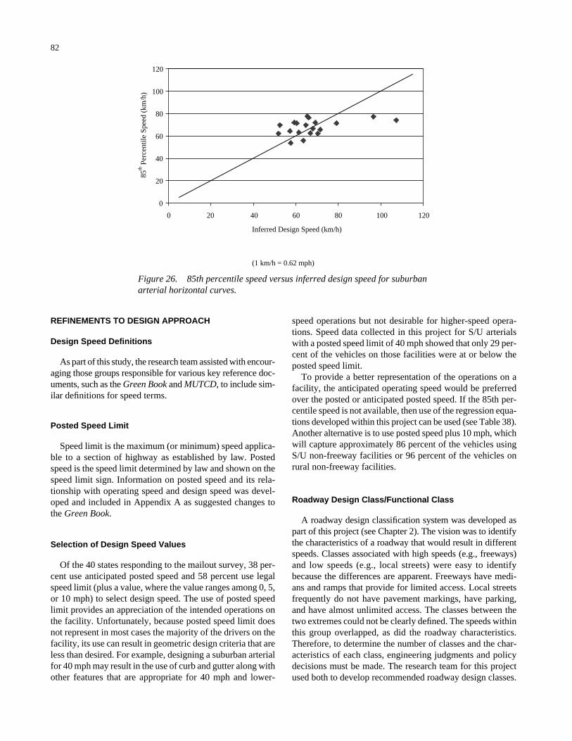
REFINEMENTS TO DESIGN APPROACH

Design Speed Definitions

As part of this study, the research team assisted with encour-aging those groups responsible for various key reference doc-uments, such as the Green Book and MUTCD, to include sim-ilar definitions for speed terms.

Posted Speed Limit

Speed limit is the maximum (or minimum) speed applica-ble to a section of highway as established by law. Postedspeed is the speed limit determined by law and shown on thespeed limit sign. Information on posted speed and its rela-tionship with operating speed and design speed was devel-oped and included in Appendix A as suggested changes tothe Green Book.

Selection of Design Speed Values

Of the 40 states responding to the mailout survey, 38 per-cent use anticipated posted speed and 58 percent use legalspeed limit (plus a value, where the value ranges among 0, 5,or 10 mph) to select design speed. The use of posted speedlimit provides an appreciation of the intended operations onthe facility. Unfortunately, because posted speed limit doesnot represent in most cases the majority of the drivers on thefacility, its use can result in geometric design criteria that areless than desired. For example, designing a suburban arterialfor 40 mph may result in the use of curb and gutter along withother features that are appropriate for 40 mph and lower-

82

speed operations but not desirable for higher-speed opera-tions. Speed data collected in this project for S/U arterialswith a posted speed limit of 40 mph showed that only 29 per-cent of the vehicles on those facilities were at or below theposted speed limit.

To provide a better representation of the operations on afacility, the anticipated operating speed would be preferredover the posted or anticipated posted speed. If the 85th per-centile speed is not available, then use of the regression equa-tions developed within this project can be used (see Table 38).Another alternative is to use posted speed plus 10 mph, whichwill capture approximately 86 percent of the vehicles usingS/U non-freeway facilities or 96 percent of the vehicles onrural non-freeway facilities.

Roadway Design Class/Functional Class

A roadway design classification system was developed aspart of this project (see Chapter 2). The vision was to identifythe characteristics of a roadway that would result in differentspeeds. Classes associated with high speeds (e.g., freeways)and low speeds (e.g., local streets) were easy to identifybecause the differences are apparent. Freeways have medi-ans and ramps that provide for limited access. Local streetsfrequently do not have pavement markings, have parking,and have almost unlimited access. The classes between thetwo extremes could not be clearly defined. The speeds withinthis group overlapped, as did the roadway characteristics.Therefore, to determine the number of classes and the char-acteristics of each class, engineering judgments and policydecisions must be made. The research team for this projectused both to develop recommended roadway design classes.

0

20

40

60

80

100

120

0 20 40 60 80 100 120

Inferred Design Speed (km/h)

(1 km/h = 0.62 mph)

85th

Perc

entil

e Sp

eed

(km

/h)

Figure 26. 85th percentile speed versus inferred design speed for suburbanarterial horizontal curves.

A part of the effort of developing the roadway design classeswas to investigate the current distribution of roadway char-acteristics. The current distribution of roadway characteris-tics supported the findings from the field studies. Roadwaysbetween a freeway and a local street have a mix of speeds andcharacteristics, with many overlaps between the classes.

83

Because freeways are easily identified as a unique classof roadway, the Green Book should include informationand discussion on its characteristics. There are chapterswithin the Green Book that include such discussions. Chapter8 covers freeways, and Chapter 10 discusses grade separa-tions and interchanges. The material in Chapter 1, however,

TABLE 41 Point where 85th percentile speed is approximately equal to inferred design speed

Point where 85th percentile speed is

approximately equal to inferred design speed

Roadway Type

Curve

Reference

km/h

mph

Rural

Vertical

Fambro et al. (15)

97 to 105

60 to 65

Two-lane rural

Vertical

Messer et al. (57)

97 to 113

60 to 70

Suburban

Vertical


90

56

Two-lane

highways

Horizontal

Chowdhury et al. (43)

90

56

Two -lane rural

Horizontal

Krammes et al. (33)

90

56

Suburban

Horizontal


70

43

Suburban

Horizontal

data available from

Texas DOT project 1769

(38)

70

43

Low-speed Horizontal Poe et al. (37) 42*

26*

* estimated from graph

1 mph = 1.61 km/h, 1 ft = 0.30 m

presents freeways as a subclass of arterial streets. To sup-port the uniqueness of freeways as a roadway class withdesign criteria that are different from both S/U and ruralarterials, we recommend that the Green Book Chapter 1 berevised to include freeways as a unique class. Therefore,information on freeways as a unique roadway class wasdeveloped and presented as suggested changes to the GreenBook (see Appendix A).

Speed Prediction/Feedback Loop

A method for ensuring that operating speeds are consid-ered within the design is to use a speed prediction model witha feedback loop. The method would predict the operating

84

speed along an alignment and then compare the speed to thedesign speed. Several countries have a more explicit consid-eration of operating speeds than AASHTO policy. The basicapproach is as follows:

• Design a preliminary alignment based on the selecteddesign speed.

• Estimate 85th percentile speeds on the alignment.• Check for large differences between 85th percentile

speeds.• Revise the alignment to reduce these differences to

acceptable levels.

The Federal Highway Administration is developing theInteractive Highway Safety Design Model (IHSDM) in an

TABLE 42 Guidelines for setting speed limits while considering design speed

Guidelines for Setting Speed Limits:

• Speed limits on all roadways should be set by an engineer based on spot speed studies and the 85th percentile

operating speed. Legal minimum and maximum speeds should establish the boundaries of the posted speed

limits. If an existing roadway’s posted speed limit is to be raised, the engineer should examine the roadway’s

roadside features to determine if modifications are necessary to maintain roadside safety.

• The 85th percentile speed is considered the appropriate speed limit even for those sections of roadway that

have an inferred design speed lower than the 85th percentile speed. Posting a roadway’s speed limit based on

its 85th percentile speed is considered good and typical engineering practice. This practice remains valid even

where the inferred design speed is less than the resulting posted speed limit. In such situations, the posted

speed limit would not be considered excessive or unsafe.

• Arbitrarily setting lower speed limits at point locations due to a lower inferred design speed is neither

effective nor good engineering practice.

• If a section of roadway has (or is expected to have) a posted speed greater than the roadway’s inferred design

speed and a safety concern exists at that location, appropriate warning or informational signs should be

installed to warn or inform drivers of the condition. Inferred design speeds slightly less than the posted speed

limit do not present an unsafe operating condition because of the conservative assumptions made in

establishing design stopping sight distances. It is important to remember that any sign is a roadside object

and that it should be installed only when its need is clearly demonstrated.

• New or reconstructed roadways (and roadway sections) should be designed to accommodate operating speeds

consistent with the roadway’s highest anticipated posted speed limit based on the roadway’s initial or ultimate

function.

Source: Fitzpatrick et al. (22)

attempt to marshal available knowledge about safety into amore useful form for highway planners and designers (52).One of the IHSDM modules is the Design ConsistencyModule. It provides information on the extent to which aroadway design conforms with drivers’ expectations. Theprimary mechanism for assessing design consistency is aspeed-profile model that estimates 85th percentile speeds ateach point along a roadway. Potential consistency problemsfor which alignment elements will be flagged include largedifferences between the assumed design speed and estimated85th percentile speed and large changes in 85th percentilespeeds between successive alignment elements.

The findings from the field studies conducted as part of thisNCHRP project could be used as a starting point for an S/Uspeed prediction model. The model could start with thespeeds predicted from the identified relationship betweenposted speed limit and operating speed. The predicted speedscould then be adjusted using developed modification factors.

85

The approach of calculating a predicted value and then mod-ifying it by using adjustment factors was employed in devel-oping an algorithm for predicting the safety performance of arural two-lane highway (58). The adjustment factors wereselected based upon available information on relationshipsbetween the geometric element and safety and the consensusof an expert panel.

Numerous studies have examined the relationships betweendesign features and operating speeds (see Appendix D). Rela-tionships identified in this project in addition to the strongrelationship between operating speed and posted speed limitinclude association of the following with lower speeds: higheraccess density, higher signal density, higher pedestrian activ-ities, the absence of centerline or edgeline markings, thepresence of parking, and the lack of a median. The relation-ships identified in this project and in other projects could be used to develop a speed prediction and feedback loopapproach to design.

86

CHAPTER 4

CONCLUSIONS AND SUGGESTED RESEARCH

CONCLUSIONS

Following the conclusions that are subdivided by the majorefforts within the project is a summary of the suggestedchanges for the next edition of the Green Book

Relationships

• Strong relationships between design speed, operatingspeed, and posted speed limit would be desirable, andthese relationships could be used to design and buildroads that would produce the speed desired for a facility.While a relationship between operating speed and postedspeed limit can be defined, a relationship of design speedto either operating speed or posted speed cannot bedefined with the same level of confidence.

• The strongest relationship found in NCHRP Project 15-18was between operating speed and posted speed limit.Except for posted speed limit, no other roadway variablewas statistically significant at a 5 percent alpha level.

• Design speed appears to have minimal impact on oper-ating speeds unless a tight horizontal radius or a lowK-value is present. Large variance in operating speedwas found for a given inferred design speed on ruraltwo-lane highways. On suburban horizontal curves, driv-ers operate at speeds in excess of the inferred designspeed on curves designed for 43.5 mph (70 km/h) orless, while on rural two-lane roadways, drivers operateabove the inferred design speed on curves designed for55.9 mph (90 km/h) or less.

• When posted speed exceeds design speed, however,liability concerns arise even though drivers can safelyexceed the design speed. While there is concern sur-rounding this issue, the number of tort cases directlyinvolving that particular scenario was found to be smallamong those interviewed in a Texas DOT study.

Mailout Survey

• A mailout survey was conducted in early 1999 to developa better understanding of what definitions, policies, andvalues are used by practicing engineers in the design ofroadways. Responses indicate that most states used the

1994 Green Book definitions (the 2000 Green Book wasnot yet published during the survey), but far fewerrespondents indicated that it was their preferred defini-tion. Therefore, there was a degree of dissatisfactionwith the 1994 definitions and their applications to thedesign process.

• Responses to Section II of the survey illustrate howdesign practices and policies can vary widely from stateto state. In selecting the design speed of a new road, thefunctional class or the legal speed limit were most com-monly used. For existing roads with few changes, eachpossible answer was chosen by between one-fourth andone-half of the respondents. In projects where the road-way is changing its functional class, the design speed fora new road of similar nature (55 percent) and the speedassociated with the functional class (47 percent) wereidentified as the most important.

• A senior designer review was part of the procedure forchecking a preliminary design, according to a largemajority (80 percent) of respondents, and reviews bythe traffic operations section were used by a little morethan one-half (55 percent) of the respondents.

• Almost all respondents (97 percent) believed that lanewidth affected drivers’ speed. Shoulder width (71 per-cent), clear zone (79 percent), presence of a raised median(61 percent), and presence of a two-way left-turn lane(66 percent) were often identified as having a perceivedinfluence on speed.

Design Element Review

• Most of the design elements and their values are eitherdirectly or indirectly selected based on design speed. Ina few situations, the type of roadway is used to deter-mine the design element value or feature; however, thetype of roadway is strongly associated with the operat-ing speed of the facility.

• The relationship with operating speed has been identifiedfor several design elements. In some cases the relation-ship is strong, such as for horizontal curves, and in othercases the relationship is weak, such as for lane width. Inall cases when a relationship between the design elementand operation speed exists there are ranges when theinfluence of the design element on speed is minimal.

87

• A third review investigated the safety implications ofdesign elements. While the relationship between a designelement and operating speed may be weak, the conse-quences of selecting a particular value may have safetyimplications. The safety review demonstrated that thereare known relationships between safety and design fea-ture and that the selection of the design feature variesbased on the operating speed of the facility. Therefore,the design elements investigated within this study shouldbe selected with some consideration of the anticipatedoperating speed of the facility. In some cases the con-sideration would take the form of selecting a design ele-ment value within a range that has minimal influence onoperating speed or that would not adversely affect safety,while in other cases the selection of a design elementvalue would be directly related to the anticipated oper-ating speed.

Previous Relationships Between Design,Operating, and Posted Speed Limit

• A late 2000 Federal Highway Administration (FHWA)research project developed regression equations that pre-dict operating speed on rural two-lane highways (36).Speed data were collected at over 200 two-lane ruralhighway sites for use in the project. Several otherresearch projects have also developed regression equa-tions to predict speeds on rural two-lane highways, espe-cially at horizontal curves. The feature that is most fre-quently identified as influencing speed on two-lane ruralhighways is horizontal curvature (degree of curve, radius,length of curve, deflection angle, superelevation, orinferred design speed). Grade, tangent length, and lanewidth have also been found to influence speed.

• Other studies have developed regression equations oridentified roadway features that affect speed on suburbanarterials and local streets. Features identified includelane width, hazard rating, access density, speed limit,roadside development, and median presence.

Field Studies

• Free-flow speed data were collected at 78 sites in S/Uand rural areas in seven cities located in six states. Foreach site, roadway and roadside characteristics werealso collected, such as number of access points withinthe study section, roadside development type, and lanewidth.

• Initial graphical evaluation provided a visual apprecia-tion of potential relationships between a roadway orroadway variable and operating speed. Findings fromthe evaluation included the following:– Posted speed limit: This has the strongest relationship

to 85th percentile speed. As posted speed increasesthe 85th percentile speed increases.

– Functional class: Local roads had the lowest speedscollected, while arterials had the highest.

– Access density (the number of access points, such asdriveways and intersections, per mile): It showed astrong relationship with 85th percentile speed, withhigher speeds being associated with lower accessdensities.

– Pedestrian activity: Lower speeds occur as pedestrianactivity increases.

– Centerline or edgeline markings: The absence ofeither is associated with lower speeds.

– On-street parking: When permitted, speeds are lower.– Median: When present, speeds are slightly lower than

when a raised, depressed, or TWLTL is present, witha few exceptions.

– Distance between features that have influence on adriver’s speed, such as a signal or sharp horizontalcurve: As the distance increases, speeds increase to apoint and then plateau.

– Shoulder width: Roadways with shoulders that havewidths of 6 ft (1.8 m) or more have speeds above 50mph (80.5 km/h), with one exception. Roadways withshoulders between 0 and 4 ft (0 and 1.2 m) also hadspeeds up to 50 mph (80.5 km/h), but most speedsobserved were lower than on the roadways with widershoulders. Roadways with curb and gutter had speedsacross the entire range seen on roadways with shoul-ders (25 to almost 60 mph [40.2 to almost 96.6 km/h]).There is no evidence that the presence of curb andgutter results in lower speeds for a facility.

– Signal density: Higher signal density is associatedwith lower speed.

– Pavement width: Fewer lower speeds are associatedwith wider pavement.

– Median width: Fewer lower speeds are associatedwith wider medians.

– Lane width: No relationship was apparent betweenlane width and speed.

– Type of residential development: Speeds on streetswith single-family residential development tended tohave lower speeds; however, some sites with residen-tial development had speeds near 50 mph (80.5 km/h).A sizeable range of speeds occurred within each devel-opment type.

• The statistical evaluation began with attempting to pre-dict operating speed using the collected roadway androadside variables. – The site variation in operating speeds is highly corre-

lated with the variation in posted speed limits.– Access density had a t-statistic greater than 1, which

corresponded to an approximate 20 percent alphalevel.

– No other roadway variable was statistically signifi-cant at the 20 percent alpha level or higher. Despitetheir low t-values, however, several variables do show

88

some sign of influence on the 85th percentile free-flow operating speed, including median type, parkingalong the street, and pedestrian activity level. Oneencouraging aspect of this analysis is that regardlessof the low t-values, most of the estimated regressioncoefficient values do have “expected” algebraic signs.This suggests that the influences of these variables onthe 85th percentile free-flow operating speed arelikely to be there, and the reason for not being able toestimate them to a good statistical accuracy is mostlikely due to the limited number of sites available foranalysis.

• A cluster analysis was performed to determine if theproject team could gain additional insight on the per-ceived influences of a roadway attribute on operatingspeed. The analysis resulted in a seven-cluster model.The following were the noteworthy features found withinthe analysis: pedestrian activity, parking, centerline,median treatment, roadside development, area type, andsignal density.

• A strong limitation with the speed relationships is theamount of variability in operating speed that exists for agiven design speed, for a given posted speed, or for agiven set of roadway characteristics.

Selection of Design Speed

• Factors used to select design speed include the following:– AASHTO: functional classification, rural versus urban,

terrain;– State DOTs: AASHTO Green Book procedure, legal

speed limit, legal speed limit plus a value (e.g., 5 or10 mph [8.1 or 16.1 km/h]), anticipated volume, antic-ipated operating speed, development, costs, and con-sistency; and

– International Practices: anticipated operating speedand feedback loop.

• Currently one-third of the responding states have usedoperating speed to select a design speed value, and one-half have used anticipated posted speed. The anticipatedposted speed implicitly considers the functional class ofthe roadway, whether it is in a rural or urban area, and,in some cases, the terrain; however, it also represents adeparture from the procedure present in the Green Book.

Operating Speed and Posted SpeedRelationships

• Several studies have demonstrated that 85th percentileoperating speeds typically exceed posted speeds. Thesestudies also show that the 50th percentile operatingspeed either is near or exceeds the posted speed limit.

• The data analyzed within this study showed that between37 and 64 percent of the free-flow vehicles on rural

roads are at or below the posted speed limit. The per-cent of vehicles at or below the speed limit is muchlower for S/U roadways (on the order of only 23 to 52percent).

• For rural non-freeway facilities, speed limit plus 10 mphwould include almost all vehicles on the roadways. ForS/U areas, speed limit plus 10 mph would only includebetween 86 and 95 percent of the vehicles on the road-ways. A much larger percentage of vehicles exceed thespeed limit on S/U non-freeway roadways than on ruralnon-freeway roadways. For the 30-, 35-, and 40-mph(48.3-, 56.3-, and 64.4-km/h) speed limits, only 28, 22,and 32 percent, respectively, of the vehicles on the roadwere at or below the posted speed limit.

• While the MUTCD recommends setting posted speedlimits near the 85th percentile speed (and the surveyssay that agencies are using the 85th percentile speedlimit to set speeds), in reality those agencies consis-tently set a majority of sites lower than the measured 85thpercentile speed by 5 mph (8.1 km/h) or more.

• Data for 128 speed study zone surveys were used in theanalysis. About one-half of the sites had between a 4-and 8-mph (6.4- and 12.9-km/h) difference from themeasured 85th percentile speed. At only 10 percent ofthe sites did the recommended posted speed limit reflecta rounding up to the nearest 5-mph (8.1-km/h) incre-ment (as stated in the MUTCD; see Table 25). At approx-imately one-third of the sites, the posted speed limit wasrounded to the nearest 5-mph (8.1-km/h) increment. Forthe remaining two-thirds of the sites, the recommendedposted speed limit was more than 3.6 mph (5.8 km/h)below the 85th percentile speed.

• Drivers’ attitude that they can drive 5 to 10 mph (8.1to 16.1 km/h) higher than the speed limit and avoid aticket does not encourage compliance with posted speed;however, neither does setting speed limits that are morethan 5 mph (8.1 km/h) from the measured 85th per-centile speed.

• Most agencies report using the 85th percentile speed asthe basis for their speed limits, so the 85th percentilespeed and speed limits should be closely matched. How-ever, a review of available speed studies demonstratesthat the 85th percentile speed is only used as a “start-ing point,” with the posted speed limit being almostalways set below the 85th percentile value by as much as8 to 12 mph.

Distributions of Roadway and RoadsideCharacteristics

• An approach to design that uses established roadwayclasses needs to provide information on acceptable rangesfor each design element. Going beyond an acceptable

89

range for a design element would theoretically commu-nicate a different roadway class (or speed environment)to the driver. To gain a better appreciation of existingconditions, roadway and roadside characteristics datafor a sample of roadways within three cities and threepredominantly rural counties were collected.

• The results for the rural roadways illustrate some note-worthy trends. – There appear to be design class relationships with

ADT, average lane width, average shoulder width,average median width, and average deflection angle.

– Less apparent from the data were expected relation-ships between design class and posted speed andbetween design class and driveway or intersectiondensity.

• The S/U roadway characteristics indicate that someexpected relationships between variables do exist, whileother anticipated relationships were not as apparentfrom the data. – Design class appears to be related to posted speed,

operating speed, presence of parking, pedestrian activ-ity, number of lanes, driveway density, intersectiondensity, signal density, and roadside development.

– Relationships between design class and lane width,median presence, or median width were anticipatedand may possibly exist, although the extent of thoserelationships is not apparent from the data.

– There are apparent relationships between posted speedrange and the following: operating speed, presence ofparking, presence of curb and gutter, average numberof lanes, lane width, median width, shoulder width,driveway density, intersection density, and roadsidedevelopment.

– The use of sidewalks does not appear to be stronglyrelated to the posted speed of the facility in the twocities.

Design Approach

• The classification of roadways into different operationalsystems, functional classes, or geometric types is nec-essary for communication among engineers, adminis-trators, and the general public. To better align designcriteria with a classification scheme, a roadway designclassification system was created. To recognize someof the similarities between the classes for the roadwaydesign class scheme and the functional classificationscheme, similar titles were used.

• Grouping freeway and local street characteristics wasstraightforward. Determining the splits for roads betweenthose limits was not as straightforward. The goal of thefield studies was to identify the characteristics that, as agroup, would produce a distinct speed. For example,what are the characteristics that would result in a high

speed and high mobility performance as opposed to thosecharacteristics that would result in a lower speed? Theresults of the field studies demonstrated that the influ-ences on speed are complex. Even when features thatare clearly associated with a local street design are pre-sent (e.g., no pavement markings, on-street parking,two lanes, etc.), 85th percentile speeds still rangedbetween 26 and 42 mph (41.8 and 67.6 km/h) for the 13sites. Such wide ranges of speeds are also present forother groupings of characteristics.

• Because of the variability in speeds observed in thefield for the different roadway classes and the large dis-tribution in existing roadway characteristics, the splitsbetween different roadway design classes need to bedetermined using a combination of engineering judg-ment and policy decisions.

Suggested Changes to the DesignApproach/Next Edition of the Green Book

• Add discussion on posted speed limit to encourage abetter understanding of the relationship between 85thpercentile speed and posted speed limit (i.e., postedspeed limits are generally set between 4 and 8 mph [6.4and 12.9 km/h] less than the measured 85th percentilespeed). Comment that between only 23 and 64 percentof vehicles operate below the posted speed limit inurban areas.

• Change text to recognize freeways as a unique func-tional class. Encourage the recognition that the look ofa roadway (e.g., ramps, wide shoulders, and medians) isassociated with the anticipated speeds on the facility.

• Add comments in the design speed discussion to iden-tify that the following may affect operating speed: radius,grade, access density, median presence, on-street park-ing, pedestrian activity, and signal density.

• Add information on the state of the practice for select-ing design speed values. Anticipated operating speedand anticipated posted speed limit are being used by anotable percentage of the states.

• Introduce the concept of speed prediction and feedbackloops. Reference the FHWA work on the IHSDM.

SUGGESTED RESEARCH

• Develop speed prediction model(s) for use in the S/U environment. Currently, FHWA is developing aspeed prediction model for rural two-lane highways aspart of the IHSDM. A speed prediction model is alsoneeded for other than two-lane highways in the ruralenvironment. The findings from the field studies con-ducted as part of this NCHRP project could be used asa starting point for an S/U speed prediction model. The

90

model could start with the speeds predicted from theidentified relationship between posted speed limit andoperating speed. The predicted speeds could then beadjusted using developed modification factors and con-sideration of signal spacing. The approach of calculat-ing a predicted value and then modifying it by usingadjustment factors was employed in developing an algo-rithm for predicting the safety performance of a ruraltwo-lane highway. The adjustment factors were selectedbased upon available information on relationshipsbetween geometric elements and safety and the consen-sus of an expert panel. The relationships identified inthis project and in other projects could use a similarapproach to develop a speed prediction and feedbackloop approach to design.

• Collect additional data to expand the speed data setdeveloped in this NCHRP study to confirm (or not con-firm) indications observed in available data. The statisti-cal evaluation in this study found only posted speed limitto be significant at a 5 percent alpha level. The only othervariable that had a t-statistic greater than 1 was accessdensity, which corresponded to an approximate 20 per-cent alpha level. Despite the low t-values obtained, sev-eral variables other than the posted speed limit do showsome sign of influence on the 85th percentile free-flowoperating speed. One encouraging aspect of the analysiswas that regardless of the low t-values, most of the esti-mated regression coefficient values did have “expected”algebraic signs. This suggests that the influences of thesevariables on the 85th percentile free-flow operating speedare likely to be there, and the reason for not being able toestimate them to a good statistical accuracy is most likelydue to the limited number of sites available for analysis.A simple calculation suggests that using the same siteselection practice, about three times more sites are neededto allow the estimates of some roadway variables toachieve a 5 percent alpha level. However, with a carefullyplanned site selection procedure following good experi-

mental design principles, the project team estimated thatthe desirable statistical level may be achievable with justone and one-half to two times more sites.

• Conduct research that emphasizes drivers’ speed choicebehaviors. For example, in this NCHRP study many ofthe speed distribution plots show three modes, indicatingthat there are perhaps three types of drivers in terms oftheir speed choices: (1) conservative drivers who alwaystry to stay below the posted speed limit, (2) moderatedrivers, who constitute the majority of the drivers, whotry not to exceed the speed limit to an unreasonabledegree, and (3) aggressive drivers, who use the postedspeed limit as the lower bound and constantly look foropportunities to drive at higher speeds. This kind ofresearch recognizes the importance of human factors indetermining driving speeds and the heterogeneity of thedriver population. Studies developed to these ends shouldbe careful to separate causality from correlation.

• Perform research that would use simultaneous equationmodeling to evaluate the speed data. The approach wouldrecognize that both posted speed limits and operatingspeeds are exogenous variables and that many variablesother than the operating speed have been used by theengineer to determine the posted speed limit. Thisresearch will require data on how the posted speed limitis determined.

• Evaluate the effects of considering the entire speed dis-tribution, instead of focusing on a particular percentilespeed in designing and operating roadways.

• Examine the roles of engineers, legislators, and enforce-ment officers in the setting of speed limits. Develop rec-ommendations on how to encourage uniformity in thesetting and enforcement of speed limits. Some of theseefforts are ongoing with current FHWA projects.

• Determine the percent of freeway vehicles in both therural and S/U environments that are driving at theposted speed limit, at the posted speed limit plus 5 mph(8.1 km/h), and at the posted speed limit plus 10 mph(16.1 km/h).

91

REFERENCES

1. Barnett, J., “Safe Side Friction Factors and SuperelevationDesign.” Highway Research Board, Proc. Vol. 16 (1936) pp.69–80.

2. Cron, F. W., “Highway Design for Motor Vehicles — A His-torical Review. Part 6: Development of a Rational System ofGeometric Design.” Public Roads, Vol. 40, No. 1 (1976) pp.9–18.

3. American Association of State Highway Officials, Policy onHighway Types (Geometric) (1940) AASHO, Washington, DC.

4. American Association of State Highway Officials, A Policy onCriteria for Marking and Signing No-Passing Zones on Twoand Three Lane Roads (1940) AASHO, Washington, DC.

5. American Association of State Highway Officials, A Policy onDesign Standards (1941) AASHO, Washington, DC.

6. American Association of State Highway Officials, A Policy onDesign Standards (1945) AASHO, Washington, DC.

7. American Association of State Highway Officials, A Policy onGeometric Design of Rural Highways (1954) AASHO, Wash-ington, DC.

8. American Association of State Highway Officials, A Policy onGeometric Design of Rural Highways (1965) AASHO, Wash-ington, DC.

9. American Association of State Highway Officials, A Policy onDesign of Urban Highways and Arterial Streets (1973)AASHO, Washington, DC.

10. Leisch, J. E., and Leisch, J. P., “New Concepts in Design-SpeedApplication.” Transportation Research Record 631, Trans-portation Research Board, Washington DC, (1977) pp. 5–14.

11. American Association of State Highway and TransportationOfficials, A Policy on Geometric Design of Highways andStreets (1984).



14. Manual on Uniform Traffic Control Devices for Streets andHighways. Federal Highway Administration, U.S. Departmentof Transportation, Washington, DC (1988).

15. Fambro, D. B., Fitzpatrick, K., and Koppa, R. J., “Determina-tion of Stopping Sight Distances.” NCHRP Report 400, Trans-portation Research Board, Washington, DC (1997).

16. Manual on Uniform Traffic Control Devices for Streets andHighways — Millennium Edition. Federal Highway Adminis-tration, U.S. Department of Transportation, Washington, DC(2000).


18. Highway Capacity Manual. Transportation Research Board,Washington, DC (1950).

19. Matson, T. M., Smith, W. S., and Hurd, F. W., Traffic Engi-neering. McGraw-Hill Book Company, Inc., New York (1955).

20. Highway Capacity Manual. Transportation Research Board,Washington, DC (1965).

21. Glossary of Transportation Terms. U.S. Department of Trans-portation, Federal Highway Administration, Washington, DC(1994).

22. Fitzpatrick, K., Blaschke, J. D., Shamburger, C. B., Krammes,R. A., and Fambro, D. B., “Compatibility of Design Speed,Operating Speed, and Posted Speed.” Final Report FHWA/TX-95/1465-2F. Texas Department of Transportation, College Sta-tion, TX (October 1995).

23. “Managing Speed: Review of Current Practice for Setting andEnforcing Speed Limits.” TRB Special Report 254, Trans-portation Research Board, National Research Council, Wash-ington, DC (1998).

24. Highway Capacity Manual, Special Report 209. TransportationResearch Board, Washington, DC (1985).



27. Tarigan, A., “Driver Performance on Horizontal Curves.” Pro-ceedings of Annual Meeting, Highway Research Board, Wash-ington, DC (1954).

28. Department of Main Roads, New South Wales. “The Behav-iour of Drivers on Horizontal Curves.” Main Roads, Vol. 34,No. 4, New South Wales, Australia (1969) pp. 127–128.

29. Emmerson, J. “Speeds of Cars on Sharp Horizontal Curves.”Traffic Engineering & Control, Vol. 11, No. 3, London (July1969) pp. 135–137.

30. McLean, J., “An Alternative to the Design Speed Concept forLow Speed Alignment Design.” Transportation ResearchRecord 702. Transportation Research Board, Washington, DC(1979) pp. 55–63.

31. Glennon, J., Newman, T., and Leisch, J., “Safety and Opera-tional Considerations for Design of Rural Highway Curves.”Report No. FHWA/RD-86/035, Federal Highway Administra-tion, Washington, DC (December 1985).

32. Lamm, R. and Choueiri, E. M., “Recommendations for Evalu-ating Horizontal Design Consistency Based on Investigationsin the State of New York.” Transportation Research Record1122, Transportation Research Board, Washington, DC (1987)pp. 68–78.

33. Krammes, R. A., Brackett, R. Q., Shafer, M. A., Ottesen, J. L.,Anderson, I. B., Fink, K. L., Collins, K. M., Pendleton, O. J., andMesser, C. J., “Horizontal Alignment Design Consistency forRural Two-Lane Highways.” Research Report FHWA-RD-94-034. Federal Highway Administration, Washington, DC (1994).

34. Islam, M.N., and P.N. Seneviratne. “Evaluation of Design Con-sistency of Two-Lane Rural Highways.” ITE Journal, Vol. 64,No. 2, Washington, DC (February 1994) pp. 28–31.

35. Poe, C. M., Tarris, J. P., and Mason, Jr., J. M., “Relationship ofOperating Speed to Roadway Geometric Design Speed,” Penn-sylvania Transportation Institute, Report Number PTI 9606(December 1996).

92

36. Fitzpatrick, K., Elefteriadou, L., Harwood, D., Collins, J.,McFadden, J., Anderson, I. B., Krammes, R.A., Irizarry, N.,Parma, K., Bauer, K., and Passetti, K., “Speed Prediction forTwo-Lane Rural Highways.” Report FHWA-RD-99-171, Fed-eral Highway Administration, Washington, DC (2000).

37. Poe, C., and Mason Jr., M., “Analyzing Influence of GeometricDesign on Operating Speeds Along Low-Speed Urban Streets:Mixed Model Approach.” Transportation Research Record1737. Transportation Research Board, Washington, DC (2000)pp 18–25.

38. Fitzpatrick, K., Carlson, P. J., Wooldridge, M. D., and Brewer,M. A., “Design Factors That Affect Driver Speed on SuburbanArterials.” Report FHWA/TX-00/1769-3. Texas TransportationInstitute, College Station, TX (August 1999).

39. Schurr, K. S., McCoy, P. T., Pesti, G., and Huff, R., “Relation-ship Between Design, Operating, and Posted Speeds on Hori-zontal Curves on Rural Two-Lane Highways in Nebraska.”Transportation Research Board. Annual Meeting. (January 2002).

40. Parma, K., “Evaluation of Alignment Indices in EstimatingTangent Speeds on Rural Two-Lane Highways.” A MastersThesis, Texas A&M University, College Station, TX (1997).

41. Dixon, K. K., Wu, C. H., Sarasua, W., and Daniels, J., “Postedand Free-Flow Speeds for Rural Multilane Highways in Georgia.”Journal of Transportation Engineering. (November/December1999) pp. 487–494.

42. Polus, A., Fitzpatrick, K., and Fambro, D., “Predicting Operat-ing Speeds on Tangent Sections of Two-Lane Rural High-ways.” Transportation Research Record 1737. TransportationResearch Board, Washington DC (2000) pp. 50–57.

43. Chowdhury, M. A., Warren, D. L., and Bissell, H., “Analysisof Advisory Speed Setting Criteria.” Public Roads, Vol. 55,No. 3 (December 1991) pp. 65–71.

44. McLean, J. R., “Speeds, Friction Factors, and AlignmentDesign Standards.” Research Report ARR 154. AustralianRoad Research Board, Victoria, Australia (1988).

45. Jessen, D. R., Schurr, K. S., McCoy, P. T., Pesti, G., and Huff,R. R., “Operating Speed Prediction on Crest Vertical Curves ofRural Two-Lane Highways in Nebraska.” TransportationResearch Record 1751. Transportation Research Board, Wash-ington, DC (2001).

46. Gattis, J. L., and Watts, A., “Urban Street Speed Related toWidth and Functional Class.” Journal of Transportation Engi-neering, Vol. 125, No. 3 (May/June 1999).

47. Liang, W. L., Kyte, M., Kitchener, F., and Shannon, P., “TheEffect of Environmental Factors on Driver Speed: A CaseStudy.” Transportation Research Record 1635. TransportationResearch Board, Washington DC (1999) pp. 155–161.

48. Rowan, J., and Keese, C. J., “A Study of Factors InfluencingTraffic Speed.” HRB Bulletin 341, Highway Research Board,Washington, DC (1962).

49. Oppenlander, C., “Variables Influencing Spot-Speed Charac-teristics—Review of the Literature.” Special Report 89, High-way Research Board, Washington, DC (1966).

50. Garber, N. J., and Gadiraju, R., “Factors Affecting Speed Vari-ance and Its Influence on Accidents.” Transportation ResearchRecord 1213, National Research Council, Washington, DC(1989) pp. 64–71.

51. Fitzpatrick, K., Nowlin, L., and Parham, A. H., “Procedures toDetermine Frontage Road Level of Service and Ramp Spac-ing.” Report FHWA/TX-97/1393-4F, Federal Highway Admin-istration, Washington, DC (August 1996).

52. Interactive Highway Safety Design Model (IHSDM): MakingSafety a Priority Online. http://www.tfhrc.gov/safety/ihsdm/brief.htm, accessed 2000.

53. Parker, Jr., M. R., “Effects of Raising and Lowering SpeedLimits on Selected Roadway Sections.” Final Report, Publica-tion No. FHWA-RD-92-084, Federal Highway Administration,Washington, DC (January 1997).

54. Parker, Jr., M. R., “Synthesis of Speed Zoning Practices.” Pub-lication No. FHWA-RD-85-096, Federal Highway Administra-tion, Washington, DC (July 1985).

55. Parker, Jr., M. R., “Comparison of Speed Zoning Proceduresand Their Effectiveness.” Final Report, prepared for the Michi-gan Department of Transportation, Lansing, Michigan, (Sep-tember 1992).

56. ITE Technical Committee 97-12, Parma, K., chair. “Survey ofSpeed Zoning Practices.” ITE Informational Report. Instituteof Transportation Engineers, Washington, DC (2001).

57. Messer, C. J., Mounce, J. M., and Brackett, R. Q., “HighwayGeometric Design Consistency Related to Driver Expectancy.”Volume II, Research Report No. FHWA/RD-81/036, FederalHighway Administration, Washington, DC (1981).

58. Harwood, D. W., Council, F. M., Hauer, E., Hughes, W. E., andVogt, A., “Prediction of the Expected Safety Performance ofRural Two-Lane Highways.” FHWA-RD-99-207, FederalHighway Administration, McLean, VA (September 2000).

A-1

APPENDIXES

The appendixes are published on the accompanying CD.Their titles and contents are as follows:

Appendix A. Suggested Changes to the Green Book.Contains suggested changes to the Green Book based on thefindings from the research project.

Appendix B. Mailout Survey. Provides the individualfindings from the mailout survey and a copy of the originalsurvey.

Appendix C. Design Element Reviews. Discusses therelationship between speed and geometric design elementsthat were evaluated in three areas: use of design speed, oper-ations, and safety. Also summarizes various definitions fordesign speed and operating speed.

Appendix D. Previous Relationships Between Design,Operating, and Posted Speed Limit. Identifies the rela-tionships between the various speed terms from the literature.

Appendix E. Field Studies. Presents the methodology andfindings from the field studies.

Appendix F. Driving Simulator Study. Presents the find-ings from a small preliminary study on driver speeds to differ-ent functional class roadway scenes.

Appendix G. Selection of Design Speed Values. Identi-fies approaches being used to select design speed within thestates and discusses approaches that could be considered forinclusion in the Green Book.

Appendix H. Operating Speed and Posted Speed Rela-tionships. Investigates how 85th percentile speed is beingused to set posted speed limit.

Appendix I. Distributions of Roadway and RoadsideCharacteristics. Identifies the distribution of design ele-ments in two cities for the field data (see Appendix E) byposted speeds and design classes.

Appendix J. Alternatives to Design Process. Presentsthe alternatives to the design process identified in Phase I ofthe research.

Abbreviations used without definitions in TRB publications:

AASHO American Association of State Highway OfficialsAASHTO American Association of State Highway and Transportation OfficialsAPTA American Public Transportation AssociationASCE American Society of Civil EngineersASME American Society of Mechanical EngineersASTM American Society for Testing and MaterialsATA American Trucking AssociationsCTAA Community Transportation Association of AmericaCTBSSP Commercial Truck and Bus Safety Synthesis ProgramFAA Federal Aviation AdministrationFHWA Federal Highway AdministrationFMCSA Federal Motor Carrier Safety AdministrationFRA Federal Railroad AdministrationFTA Federal Transit AdministrationIEEE Institute of Electrical and Electronics EngineersITE Institute of Transportation EngineersNCHRP National Cooperative Highway Research ProgramNCTRP National Cooperative Transit Research and Development ProgramNHTSA National Highway Traffic Safety AdministrationNTSB National Transportation Safety BoardSAE Society of Automotive EngineersTCRP Transit Cooperative Research ProgramTRB Transportation Research BoardU.S.DOT United States Department of Transportation

NCHRP Report 504 – Design Speed, Operating Speed, and ...

Documents

Transcript of NCHRP Report 504 – Design Speed, Operating Speed, and ...