NBS-M016 Contemporary Issues in Climate Change and Energy …
35
NBS-M016 Contemporary Issues in Climate Change and Energy 2010 A Domestric Hot Water System Lecture Handout 4 Section 22 Introduction to Renewables Section 23 Solar Energy Section 24 Wind Energy Section 25 Tidal Energy A Darrieus Rotor
Transcript of NBS-M016 Contemporary Issues in Climate Change and Energy …

NBS-M016 Contemporary Issues in Climate
Change and Energy 2010
A Domestric Hot Water System
Lecture Handout 4
Section 22 Introduction to Renewables
Section 23 Solar Energy
Section 24 Wind Energy
Section 25 Tidal Energy
A Darrieus Rotor

N. K. Tovey NBS-M016 Contemporary Issues in Energy and Climate Change 2010 Section 22
22. RENEWABLE ENERGY RESOURCES.
22.1 ORIGINS OF RENEWABLE ENERGY
RESOURCES
Renewable energy sources may be divided into three
categories as was discussed in Section 4.
1) Solar -
a) direct
b) indirect - e.g. wind, waves., biomass
2) Lunar - tidal
3) Geothermal
Of these, both direct and indirect solar sources are about
50000 times the geothermal resource, and 500000 times the
lunar source.
As revision you should consult section 4 of of the notes for
the magnitudes of the different sources.
Often included in the heading of Renewable Energy is Energy
from Waste. Sometimes such energy is linked with biomass.
It is perhaps more correctly to consider this as an alternative
Energy Source. Thus PET COKE is now often being used in
the Cememnt industry and also Iron and Steel. While an
alternative fuel it has an even higher carbon factor than coal
The subject of Renewable \Energy is vast and a brief overview
was given earlier in the course in Section 4. Two specific
topics will be covered explicitly in more depth: Solar and
Wind, although notes are also included for tidal as this has
recently ( 2009) been the subject of a Government
Consultation.
23. SOLAR
23.1 Introduction The sun behaves as a nearly perfect BLACK BODY
radiator at a temperature of 6000K generated from
nuclear fusion.
it emits a continuous spectrum from 200nm (ultra-
violet), through visible light (400 - 800nm) to infra-red
(up to 3000nm).
Outside earth's atmosphere, the intensity of solar
radiation is 1395 Wm-2, although this may vary by up to
+_ 5% as a result of sun spot activity, and from the
variation in the distance of the sun from the earth.
Absorption by the atmosphere (which is more significant
at certain wavelengths) reduces value by about 28% to
1000 W-2 on a horizontal surface directly below the sun.
Reduction for more northerly latitudes is not that great
provided that collector is tilted perpendicular to the sun.
Thus in UK a values of 800+ Wm-2 can be achieved on a
clear day in summer.
Much more significant in reducing the levels are the
climatic conditions.
Typical annual averages:-
UK 8 MJm-2
(about 93 Wm-2 - up to 115 Wm-2 in in SE)
France (South) 14 MJm-2 (about 162 Wm-2)
Australia 16 MJm-2 (about 185 Wm-2)
India 20 MJm-2 (about 231 Wm-2)
Solar radiation has two components:-
a) direct - a direct line of sight from sun to place in
question.
b) indirect (or diffuse)- solar radiation from reflections
from the ground, atmosphere, clouds etc.
Indirect radiation is always present during daylight hours.
Direct radiation is present only when sun is not obscured
by cloud. Diffuse radiation on a clear day is less than
diffuse radiation on a cloudy day. Thus in summer,
north facing windows receive more solar gain on a cloudy
day than on a clear day.
Unlike many countries, the direct component is relatively
small - only 45% in summer, and about 35% in winter.
Nevertheless up to 80 Wm-2 is still received during the
day time on a dull winters day in the UK.
Applications in situations where direct component is a
major part of total radiation:-
1) direct electricity generation from photo- voltaic
cells. BP have developed a refrigerator/freezer for
the storage of vaccines in Third World countries.
2) Indirect electricity generation by raising steam. e.g.
Paris exhibition 1879, Egypt 1913, Bairstow,
California 1982.
3) Adsorption cycle refrigerators, freezers, and air-
conditioners.
4) Solar cooking. e.g. China, India.
5) Special applications - metallurgical etc., Odeillo,
France.
6) Centralised Power Plants – e.g. Bairstow, California,
Gila Bend, Arizona, Seville, Spain.
Most direct applications require focusing or semi-
focusing collectors which must be tracked with the sun
either automatically or manually. For some applications,
some types of manual tracking collector need only be
adjusted once a week.
In UK, most applications will be for low temperature
heating requirements e.g. hot water/ space heating.
Diffuse radiation can be collected with stationary flat-
plate collectors, and thus do not require frequent
attention either for periodic tracking adjustments or for
servicing.

N. K. Tovey NBS-M016 Contemporary Issues in Energy and Climate Change 2010 Section 23
105
23.2 Active and Passive systems
Systems which deliberately collect solar radiation
such as any of the devices listed above are known as
ACTIVE SOLAR DEVICES.
PASSIVE SOLAR ENERGY applications include
incidental solar heating (or cooling) of buildings
from architectural design, crop drying, drying washing, etc. Greenhouses are a particular
architectural which exploits PASSIVE SOLAR
ENERGY.
Some people also include in the group PASSIVE,
those hot water heaters etc. which operate on a
thermosyphon and thus have no moving (ACTIVE)
parts.
23.3 Summary of Solar Energy
Solar
Radiation
Deliberate
Collection
Incidental Collection
Unfocussed
Focused Architectural Design
Biomass
flat plate
collectors/
solar ponds
parabolic or tracking
planar collectors (with
or without extra
lenses/mirrors)
water/space
heating
High temperature
R & D
heating / cooling
Process Heat
Power generation
greenhouses
crop drying
Fig. 23.1 Summary of Solar Energy
23.4 Passive Solar Energy - heating.
Solar energy (both direct and diffuse) falling on a object will
cause it temperature to rise until there is a balance between
the heat gained and the heat lost. A small proportion of the
incoming radiation will also be reflected from the surface.
WALLS AND ROOF - often rise to a temperature ABOVE the
surrounding air-temperature in direct sunlight, and this may
cause some heat to flow inwards. Can be significant in hot
climates. [Note: the need to insulate buildings in hot climates
to prevent heat gain is often over-looked - it is as important as
insulation of buildings to retain heat in cold climates].
Indeed problems of overheating are now becoming an issue
even in the UK.
WINDOWS - a significant proportion (about 80 - 85% in the
case of single glazing) is transmitted directly to the interior
where it will be absorbed by the contents of the room.
However, the heat energy given off by these objects is of a
much longer wavelength, and a large proportion of this heat
will be internally reflected by the glass, and will thus be
'trapped'.
On a CLEAR day in the depth of winter a south facing room
with large windows can be self sufficient in energy during
daylight hours even in the UK. However, for the 17+ hours of
darkness, such large windows would cause increased heat
losses. Such windows, however, will often lead to over
heating in summer
A BALANCED ARCHITECTURAL DESIGN IS
NEEDED TO GIVE OPTIMUM IN FUEL SAVING.
NOTE:-
For SOUTH facing windows, maximum solar gain occurs in
March/April and August/September. The sun is too high in
the sky in June and a higher proportion of incoming sunlight is
reflected. This can help to reduce overheating in summer.
However, overheating in SOUTH facing rooms in summer can
occur even in the UK unless overhanging shading is
provided.

N. K. Tovey NBS-M016 Contemporary Issues in Energy and Climate Change 2010 Section 23
106
23.5 Architectural Features to enhance Passive Gain.
1) Minimise north facing window area
2) Maximise south facing window area and provide
these rooms with SOLID uncarpeted floors e.g.
polished timber or tiles. Alternatively provide a
conservatory on south side of house.
3) Place most heavily used rooms, or rooms with lowest
activity levels to south of building.
4) Provide inter room ventilation by mechanical means,
and provide automatic ventilation of conservatories
to avoid overheating in summer.
5) Provide an overhang over south facing windows and
shelter conservatories to minimise overheating in
summer. One method is to plant deciduous trees.
In winter the shading is limited, but in summer
when in full leaf, significant shading can be
provided. But trees close to property can cause
foundation problems.
6) Provide a Trombe Wall behind a glazed front wall, but
ensure adequate ventilation is provided for summer.
Some Examples of Passive Solar Design and
associated problems
A Passive Design incorporating a Trombe Wall construction
includes the old people's homes in Bebbington which were
designed jointly by Pilkington Glass and Merseyside
Development Corporation. Success of design depends on
CORRECT operation of vents A - E These were often set
incorrectly by the occupants.
A second house - The Marseille House also incorporates a
series of slats which had to opened and closed correctly.
A School in Wallesey requires no active heating (see separate
sheet). Heat from lighting and body heat supplement solar
gain through a double skinned glass wall. Part of internal
layer is constructed of reversible aluminium slats - black
outwards in winter, shiny side outwards in summer. Air
temperatures range from 17oC in winter to 24oC in summer,
although summertime radiant temperatures sometimes reaches
uncomfortable levels over 28oC.
Passive solar cooling can be achieved in dry climates by
inducing a flow of air through the house. The incoming
air passes over damp cloths and this cools the air as the
water evaporates. Temperature depressions of 5 - 10oC
are possible.
Fig. 23.2 A Trombe wall house of the design used in
Bebbington scheme.
Fig. 23.3 Passive Solar Cooling
Fig. 23.4 Example of Passive Solar Cooling and Passive Solar Heating in a European style house.

N. K. Tovey NBS-M016 Contemporary Issues in Energy and Climate Change 2010 Section 23
107
The “sun space” serves as a collector in winter when the solar
shades are open and as a cooler in summer when the solar
shades are closed. Thick concrete walls modulate wide swings
in temperature by absorbing heat in winter and insulating in
summer. Water compartments provide a thermal mass for
storing heat during the day and releasing heat at night.
However, frequently in summer, adequate cooling does not
occur and buildings overheat – e.g. the so called “low Energy”
Building at Chingwa University in Beijing.
23.6 ACTIVE SYSTEMS - Flat Plate Collectors
1) Thermosyphon - hot water storage cylinder must be
above top of collector.
Fig. 23.5 A thermosyphon solar collector
NOTE: The contra-flow system in the tank to ensure
maximum efficiency
2) Pumped Systems: same basic diagram except water is
pumped around circuit, and cylinder can be below
collector. However, active controls must be present to
ensure hot water is not pumped to radiate heat from
collector at night time.
3) Pumped Trickle Type Collectors - these collectors allow water to run down in grooves
under gravity. Some experiments have been made with
additives to make water black and improve absorption.
All water runs by gravity over the collector.
Fig. 23.6. A trickle type collector - NOTE: contra flow
system through tank
4) Indirect Systems - use two storage cylinders, one for
solar circuit to preheat the water before going into
conventionally heated hot water cylinder.
Solar Heating pre-heats incoming hot water and can be
used even if the temperature rise is small.: NOTE the
contra flow heat exchangers in both tanks.
Fig. 23.7 An indirect solar heating system
Fig. 23.8. The Broadsol variant of indirect solar heating
5) Tubular Flat Plate Collectors - these consist of a
series of glass tubes at the centre of which is a pipe
conducting the working fluid. Some such schemes have
evacuated tubes which reduce heat losses from collectors.
Fig. 23.9 The problem with flat plat collectors is that unless
they are aligned perpendicular to the sun, the reflectivity of
the cover glass can be high reducing the effective amount of
energy available.

N. K. Tovey NBS-M016 Contemporary Issues in Energy and Climate Change 2010 Section 23
108
Fig. 23.10 Tubular collectors
With a tubular collects, the sun is perpendicular to the glass
surface for a wide range of azimuth angles, and
thus reduces reflection. compared to flat plate collectors.
Fig. 23.11 An array of tubular collectors
Note: spacing between tubes is necessary to exploit full
potential and this does reduce the effective collector area.
Tubular collectors may be 3-%% more efficient..
23.7 Solar panels with combi-boilers.
Most combi boilers specify that they must have cold water as
input and are unsuitable for using with a solar tank,
particularly as in summer the tank water can reach over 60oC.
A few combi boilers do allow solar preheating using a system
shown in Fig. 23:12
Fig. 23.12. A solar pre-heating system with a combi boiler
NOTE: Most combi boilers do not allow solar pre-heating –
contact the manufacturer.
23.8 Advantages and disadvantages of different types
of flat plate collector.
1) Thermosyphons must have cylinder perched at apex of
roof. In many houses there may be inadequate room.
Care must be taken with pipe work runs to ensure free
circulation.
2) Pumped systems require pump energy. It is normal to
delay switching on system until collector temperature is
at least 3oC warmer than water in cylinder.
3) Provision must be made to avoid water in collector from
freezing. - remember the collector may be several
degrees colder than the air temperature on a clear night.
Collectors should contain anti-freeze or should be
drained.
4) Thermosyphons cannot be drained conveniently. Trickle
systems are the best as they automatically drain when
pump is switched off.
5) Direct systems cannot be used if anti-freeze or other
additives are present. Further if water temperature is not
high enough, then the storage tank becomes an ideal
breeding ground for Legionnaires Disease bacteria.
6) Indirect systems are convenient in that topping up by
conventional sources can be done.
7) Tubular collectors improve efficiency somewhat, but
seasonal performance of all collectors will not exceed
about ~40% - 50%
(DESPITE MANUFACTURER'S CLAIMS!).
NOTE: Collectors are most efficient if they raise the water
temperature by only a few degrees. Double glazing
REDUCES efficiency unless high temperatures >80oC are
used.
23.9 Some Resuts from the Broadsol Project
The Broadsol Project was initiated by a consortium including
UEA, Broadland District Council and CML Contracts who
did the installation.
The aim was to involve the community and ultimately 40
householders had panels attached to their properties with 19
of them being monitored.
Fig. 23.13 Broadsol installation in Norwich
Over the year one installation achieved 911.562 kWh despite
manufacturers claims that the figure would be higher. Some
interesting things emerge.
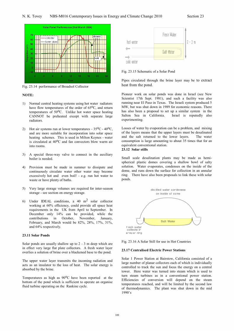
Up to 7+ kWh can be achieved on a sunny day – more than
sufficient for requirements. Even on a March day (March 2nd
2004) when there was snow on the ground, a temperature of
59oC was achieved. This was more than sufficient for a
childs bath and an adult shower that evening – see Fig. 23.14
23.10 Applications of active systems to space heating.
In Milton Keynes a house has been designed to use an active
hot water system to assist in space heating (see separate
sheet). A 43 m2 collector feeds two 2.5 m3 storage tanks
situated centrally in the house. Computer simulations
suggested that 30% savings could be achieved
Cold Water in
Cold Water in
N. K. Tovey NBS-M016 Contemporary Issues in Energy and Climate Change 2010 Section 23
109
Fig. 23.14 performance of Broadsol Collector
NOTE:
1) Normal central heating systems using hot water radiators
have flow temperatures of the order of 65oC, and return
temperatures of 50oC. Unlike hot water space heating
CANNOT be preheated except with separate large
radiators.
2) Hot air systems run at lower temperatures - 35oC - 40oC,
and are more suitable for incorporation into solar space
heating schemes. This is used in Milton Keynes - water
is circulated at 40oC and fan convectors blow warm air
into rooms.
3) A special three-way valve to connect in the auxiliary
boiler is needed.
4) Provision must be made in summer to dissipate and
continuously circulate water other water may become
excessively hot and even boil! - e.g. run hot water to
waste or have plenty of baths.
5) Very large storage volumes are required for inter-season
storage - see section on energy storage.
6) Under IDEAL conditions, a 40 m2 solar collector
working at 60% efficiency, could provide all space heat
requirements in the UK from April to September. In
December only 14% can be provided, while the
contributions in October, November, January,
February, and March would be 82%, 28%, 17%, 31%,
and 64% respectively.
23.11 Solar Ponds
Solar ponds are usually shallow up to 2 - 3 m deep which are
in effect very large flat plate collectors. A fresh water layer
overlies a solution of brine over a blackened base to the pond.
The upper water layer transmits the incoming radiation and
acts as an insulator to the loss of heat. The solar energy is
absorbed by the brine.
Temperatures as high as 90oC have been reported at the
bottom of the pond which is sufficient to operate an organise
fluid turbine operating on the Rankine cycle.
Fig. 23.15 Schematic of a Solar Pond
Pipes circulated through the brine layer may be to extract
heat from the pond.
Pioneer work on solar ponds was done in Israel (see New
Scientist 17th Sept. 1981), and such a facility was also
running near El Paso in Texas. The Israeli system produced 5
MW, but was shut down in 1989 for economic reasons. There
has also been a proposal to set up a similar system in the
Salton Sea in California. Israel is reputedly also
experimenting.
Losses of water by evaporation can be a problem, and mixing
of the layers means that the upper layers must be desalinated
and the salt returned to the lower layers. The water
consumption is large amounting to about 35 times that for an
equivalent conventional station.
23.12 Solar stills
Small scale desalination plants may be made as hemi-
spherical plastic domes covering a shallow bowl of salty
solution. Water evaporates, condenses on the inside of the
dome, and runs down the surface for collection in an annular
ring. There have also been proposals to link these with solar
ponds.
Fig. 23.16 A Solar Still for use in Hot Countries
23.17 Centralised Electric Power Stations
Solar 1 Power Station at Bairstow, California consisted of a
large number of planar collectors each of which is individually
controlled to track the sun and focus the energy on a central
tower. Here water was turned into steam which is used to
turn steam turbines as in a conventional power station.
Efficiencies of conversion will depend on the steam
temperatures reached, and will be limited by the second law
of thermodynamics. The plant was shut down in the mid
1990’s

N. K. Tovey NBS-M016 Contemporary Issues in Energy and Climate Change 2010 Section 23
110
Fig. 23.17 A centralised power station:- each reflector must
be steered individually to track the sun.
Other systems have been the SEGS series which have
included a small natural gas boiler so that super-heating can
be done - thereby improving efficiency.
Future developments suggest linking a combined cycle gas
turbine with a centralised solar power station. The exhaust
from the gas turbine would be used primarily for superheating
and reheating, and finally the feed water heating, whereas
the solar system would transfer the heat needed in
evaporation. This latter is a limitation in conventional
CCGT's as the
temperature difference varies along the heat exchanger. Using
such a combination can boost the overall efficiency of a CCGT
by 5%+
To supply all the electrical requirements of the USA about
12500 sq km of the Arizona Desert would be required
(assuming a conversion efficiency overall of 10%), and this
would involve a huge investment in materials.
A very good review of the subject is included in Renewable
Energy by Johansson, Kelly, Reddy, and Williams - pages
222-290.
23.18 Thermionic Generators
When an electrode is heated (by solar or other means) some
electrons will gain sufficient energy to escape. If a second
electrode is placed close to the first and is cooled, then a
current can be induced to flow in an external circuit
connecting the two electrodes.
Fig. 23.18 A Thermionic Generator
23.19 Photo-voltaic cells
Semiconductors doped with minute quantities of certain
elements (e.g. 1 part per million) can be arranged in pairs to
generate electricity when irradiated by solar radiation.
Fig. 23.19 Schemtaic of A Photo-Volatic Cell
The first type - the "N" - type consists of an element such as
silicon doped an element with one additional electron - e.g.
arsenic. The second or "P" type has a doping element with
one fewer electron - e.g. boron.
Made up into a sandwich, of one "P" layer overlying one "N"
layer these will generate an open circuit voltage of about 0.6
Volts, at an efficiency of about 15%.
Gallium Arsenide and Cadmium Sulphide will probably
eventually give practical efficiencies of about 25%.
Theoretically, the efficiency is about 30%.
Only wavelengths shorter than 1100 nm are effective, longer
wavelengths only produce heating of device which reduces
efficiency.
Costs of photo voltaic cells. The following prices were often
cited in the 1990s
$ per peak
watt
1961 175
1973 50
1975 20
1986 5 - 6
1991 4 - 5
1994 3 - 4
However, the reduction is cost does not seem to have been
continued as there are references to current 2010 prices in the
range of $4 - $6 per peak watt – and some current website are
even quoting prices as high as $8-$10 per peak watt. These
prices compare with around
$1.2 - $1.8 for coal
$2.0 - $ 2.3 for a PWR,
$0.8 for a CCGT
and $1.5 – 1.8for onshore wind
Note: for the fossil fuel these costs are only the capital costs,
and do not include running costs - i.e. fuel costs).
Scope for much further reduction in price seems somewhat
limited except for small scale applications - possibly

N. K. Tovey NBS-M016 Contemporary Issues in Energy and Climate Change 2010 Section 23
111
eventually to $2 - $3. For example isolated farmsteads etc.
applications in Third World for freezers/refrigerators.
The University of Northumbria installed a 40 kW photo-
voltaic generator on the side of a building in 1994. Several
others followed – including the ZICER building in 2003.
That building produces ~22000kWh a year from a 34 kWp
array implying a load factor of 8%.
23.20 Solar Satellite Power Stations.
Outside earth's atmosphere in geostationary orbit, sun never
sets, there is no absorption by atmosphere, and no clouds.
Satellite Power Stations would collect energy and convert it
into a microwave beam for transmission to earth where energy
would be reconverted to electricity with an efficiency of about
80%.
Present schemes suggest placing giant solar modules in
geosynchronous earth orbit. To produce as much power as five
large nuclear power plants (1 billion watts each) several
square miles of solar collectors, weighing 10 million pounds,
would have to be assembled in orbit; an earth-based antenna 5
miles in diameter would be required. Smaller systems could
be built for remote islands, but the economy of scale suggests
advantages to a single large system
Power density in microwave beam as it heats earth would be
beam would be 23 mW cm-2 at centre falling to 1 mW cm-2 at
edge.
Exclusion zone necessary around each receiving site in case
beam goes off "target". Also fail safe devices are proposed to
disperse beam in fault conditions.
Standards of microwave exposure:-
10 mW cm-2 in USA
but only 0.1 mW cm-2 in USSR.
23.21 Ocean Thermal Energy Conversion (OTEC)
In tropics sea surface temperature is 25oC or higher while at
a depth of 500m it is about 5oC.
Large potential - e.g. in Gulf Stream off Florida, but this
might affect climate of northern Europe.
This temperature difference can be exploited using second law
of thermodynamics.
Warm surface water is used to boil a fluid such as ammonia
(or very low pressure steam) which then expands through a
turbine and condensed by the supply of cold water.
As low temperatures are involved, the efficiency of conversion
is low (about 1 - 2%).
Enormous volumes of water must be pumped from depth in
normal operation of such a plant.
Generally non-polluting, but plant must be moored in deep
water. Hence there are problems in transmitting power
ashore. Suggestions have been made to use electricity to
electrolyse water and pump the hydrogen ashore as a fuel in
its own right.
Scheme first proposed in 1880, and first one built was off
Cuba in 1929.
Second scheme off West Africa in 1950s (3.5MW). This
scheme improved fishing in area as nutrients from deep ocean
were brought to surface.
Current scheme (50MW) is in operation off Hawaii.
23.22 Biomass possibilities
Plants collect solar energy, and convert them into a form
which might be used as a fuel - e.g. peat, wood etc.
In developed world, wood is being used faster than it is
planted, so such schemes would need massive planting, and
thus be in competition with areas used for food production, or
alternative scrub land could be used. Once again there is a
substantial environmental impact.
However, on steep slopes, planting of trees could minimise
soil erosion and could be an additional benefit.
Other plants such as sugar beet, water hyacinth etc. can be
used, but are probably most effective if they are digested or
fermented into a secondary fuel.
anaerobic digestion (oxygen free conditions) can produce
biogas which is largely methane, but also contains CO2 which
is often removed to provide a fuel of higher calorific value.
Many sewage works in UK treat their sewage in this way.
However, temperature must be kept above 34oC, and a large
proportion of energy is required in heating. In countries such
as India and China small scale digesters are in widespread
use, particularly where there are many animals.
On livestock farms in UK it could be a very appropriate form
of energy.
Fermentation - Yeast can be used to break down
carbohydrates in plants to form alcohols. It is used
extensively in Brazil where the alcohol is used as a petrol
substitute. - but see issue of New Scientist January 1993
which suggests that Brazil may be moving away from this in
favour of oil.
Sugar cane is crushed an allowed to ferment. After
distillation the liquid is 95% alcohol, and this is blended to
give Gasohol (20% alcohol and 80% petrol). New engines
could run off alcohol alone.
Advantages and Disadvantages of Biomass for UK
Advantages
1) Techniques well developed e.g. in Brazil.
2) Plants collect AND store energy.
3) Non-polluting.
Disadvantages
1). Energy used in collecting crops and in processing is
not known wil a high degree of accuracy, and there
are some who say that the energy requirements of
maintenance and harvesting mean that the source is
not a net energy producer (however look at practical
notes). We must be sure that scheme will be a net
producer of energy.

N. K. Tovey NBS-M016 Contemporary Issues in Energy and Climate Change 2010 Section 23
112
2). Biomass production would compete with food
production.
thus of Land in UK:- about 75% of land is
currently not built up or in conservation areas,
and if all non-built up or mountainous regions
were used exclusively for biomass, then only
12% of UK energy needs could be produced
by this means.
Three biomass plants are now in operation in East Anglia, but
all of these are really using agricultural wastes as the fuel.
The UEA system will use an advanced gasification technique
combined with combined heat and power. The largets
biomass power stations are around 20 – 30MW in size
compared to up to 4000 MW for a single coal fired power
station.
23.23 Economics of Solar Hot Water Heaters in UK.
Current cost is around £3500 - £4000, of which around £600 +
is for a replacement cylinder and typically £1500 for
installation. The cheaperst would be around £3000, but
some suppliers are quoting over £6000. We shall assume
£3,500 in our calculations.
A large household uses 140 litres of hot water each day at a
temperature of 55oC.
Inlet water temperature is 10oC.
so energy required = 140 x 4.1868 x (55-10) kJ/day
= 9.63 GJ/annum
=============
For gas heating, seasonal efficiency for hot water is about
60%
so delivered energy requirement is:- 9.63/0.6
= 16.05
GJ/annum
=============
Cost of gas in Feb 2009 varies from around 2.6p per kWh for
high useage to over 6p for low usage, with a typical weighterd
average for those with gas central heating of around 3.5p
Or around £10.03 per GJ
So current annual running cost is 16.05 x 9.72 = £156
======
A 2.6 m2 solar collector would provide 40 - 50% of total
requirement. Assume 50%, so saving is £78 per annum.
[This is probably an over estimate of saving as the saving is
more to do with the sequence of use rather than any technical
matter]. Thus if people have showers/baths in the morning,
there will be much less saving than if they have them late
morning etc.]
So net present value at 0% discount rate, using a lifetime of
the collectors of 20 years is 20 x 78 - 3500 = - £1940, and
so is far from cost effective.
With full rate electricity at prices ranging from 11p – 16p per
kWh for the second tier about and up to 26p for the first tier
rate, the weighted average cost per unit of full rate electricity
appears to range from 13.5 – 14.5p (say 14p) per kWh. This
rewpresents 7.60p per kWh (– Jan 2005 average of two tier
rate) or about £38.90 per GJ. For electricity we must
remember that the heating at point of end use is 100%
efficient and thus the total annual cost will be 9.63 *38.90 =
£375 and the saving from a solar collector may be estimated at
£187.50 per year or around £3700 over 20 years giving a small
net present value overall of +£200.
At a discount rate of 5%, the cumulative discount for 20 years
(year 0 + 19 years of discounting) is 13.085319 (see table
below) so the total effective saving for full rate electricity is
now only 13.085319 x 187.50 = £2453.50 making it even less
attractive as the NPV is now -£1046.50 in the case of
electricity.
In practice the savings will not actually be 50% as energy is
consumed in the pump. For full rate electricity, the scheme
would still be just cost effective over 20 years assuming no
discounting, but with a typical discount rate of 5%, the
installation price would have to be no greater than £2000.
In the case of gas, the price would have to be no more than
£1400 to be cost effective at 0% discount rate, but at 5%, the
price would have to be under £1000. Unfortunately even
with mass production, the labour installation charges are still
likely to be equal to this price even if the components were
free. On the other hand if the collectors were installed at the
tiem of initial house construction, the labour charges could be
much less and could then be just about cost effective even for
gas. Even if soalr heaters are not installed initially, if dual
circuit cylinders were mandatory, then this would probably
shave up to £1000 of the cost of installationb of a complete
system.
With mass production, the cost of all the components could
probably be brought down to about £ 500 for the collector,
£80 for tank, £40 for pump, £40 for pipe work and fittings or
a total of £660, but the installation charge would still remain
at around £1000, giving a total cost of £1660. Even then the
scheme is not cost effective over 20 years under current gas
fuel costs even with 0% discount rate.. [cost £1660 – saving
£1560]
If Government were to invest money (i.e. subsidise the
installations such that they just became cost effective over 10
years over 5% discount rate – it is questionable whether
people would consider things over a longer period) then the
total cost if electricity were the fuel should not be greater than
£1520, i.e. a subsidy of £140 for electrically heated
installation), but for gas the total cost after subsidy and any
discounting indicated above would have to be no more than
£632, or a subsidy of £around £1000 per collector.
To install collectors on all the suitable domestic properties
(i.e around 15 million out of 23 million) and using this
subsidy figure would involve an investment of £0.5 billion
pounds per annum and £15 billion pounds in total. Remember
that electric heating of hot water only constitutes a small
proportion, although the Government should perhaps
introduce a differential subsidy depending on fuel type used.?
We can estimate a possible installation rate assuming that
financial barriers were not a limitation. Currently only about
10000 collectors are installed a year although this figure is
now increasing. Let us assume that a concerted effort is made
with a target in the first year of 50000 units raising by 50000 a
year for 10 years until half a million are installed each year as
the market would start to see saturation effects. We shall
N. K. Tovey NBS-M016 Contemporary Issues in Energy and Climate Change 2010 Section 23
113
neglect the issues relating to replacement collectors and
concentrate only on new installations beginning in 2009 and
continuing for 35 years when all 15 million suitable houses
would be equipped. With 250 working days in each year, and
each collector requiring 2 people for 2.5 days to install some
1000 people would need to be employed initially solely in the
installation with perhaps 50% of that number in sales,
distribution, ordering, purchasing. In addition there would
perhaps be a further 1500 involved in manufacture making
around 3000 in total which would rise to 30000 by yerar 10
giving sufficient time to develop the necessary skills base.
DISCOUNT TABLE FOR 5% DISCOUNT RATE
Present value of
£1 Cumulative present
value of £1
0 1 1
1 0.952381 1.952381
2 0.907029 2.85941
3 0.863838 3.723248
4 0.822702 4.54595
5 0.783526 5.329476
6 0.746215 6.075691
7 0.710681 6.786372
8 0.676839 7.463211
9 0.644609 8.10782
10 0.613913 8.721733
11 0.584679 9.306413
12 0.556837 9.863250
13 0.530321 10.393571
14 0.505068 10.898639
15 0.481017 11.379656
16 0.458112 11.837768
17 0.436297 12.274065
18 0.415521 12.689585
19 0.395734 13.085319
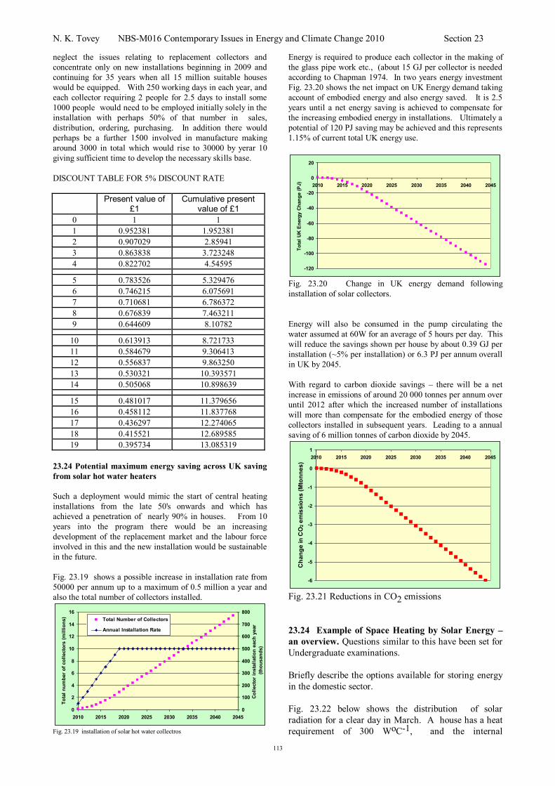
23.24 Potential maximum energy saving across UK saving
from solar hot water heaters
Such a deployment would mimic the start of central heating
installations from the late 50's onwards and which has
achieved a penetration of nearly 90% in houses. From 10
years into the program there would be an increasing
development of the replacement market and the labour force
involved in this and the new installation would be sustainable
in the future.
Fig. 23.19 shows a possible increase in installation rate from
50000 per annum up to a maximum of 0.5 million a year and
also the total number of collectors installed.
0
2
4
6
8
10
12
14
16
2010 2015 2020 2025 2030 2035 2040 2045
To
tal
nu
mb
er
of
co
llecto
rs (
mil
lio
ns)
0
100
200
300
400
500
600
700
800
Co
llecto
r in
sta
llati
on
each
year
(th
ou
san
ds)
Total Number of Collectors
Annual Installation Rate
Fig. 23.19 installation of solar hot water collectros
Energy is required to produce each collector in the making of
the glass pipe work etc., (about 15 GJ per collector is needed
according to Chapman 1974. In two years energy investment
Fig. 23.20 shows the net impact on UK Energy demand taking
account of embodied energy and also energy saved. It is 2.5
years until a net energy saving is achieved to compensate for
the increasing embodied energy in installations. Ultimately a
potential of 120 PJ saving may be achieved and this represents
1.15% of current total UK energy use.
-120
-100
-80
-60
-40
-20
0
20
2010 2015 2020 2025 2030 2035 2040 2045
To
tal
UK
En
erg
y C
han
ge (
PJ)
Fig. 23.20 Change in UK energy demand following
installation of solar collectors.
Energy will also be consumed in the pump circulating the
water assumed at 60W for an average of 5 hours per day. This
will reduce the savings shown per house by about 0.39 GJ per
installation (~5% per installation) or 6.3 PJ per annum overall
in UK by 2045.
With regard to carbon dioxide savings – there will be a net
increase in emissions of around 20 000 tonnes per annum over
until 2012 after which the increased number of installations
will more than compensate for the embodied energy of those
collectors installed in subsequent years. Leading to a annual
saving of 6 million tonnes of carbon dioxide by 2045.
-6
-5
-4
-3
-2
-1
0
1
2010 2015 2020 2025 2030 2035 2040 2045
Ch
an
ge
in
CO
2 e
mis
sio
ns
(M
ton
ne
s)
Fig. 23.21 Reductions in CO2 emissions
23.24 Example of Space Heating by Solar Energy –
an overview. Questions similar to this have been set for
Undergraduate examinations.
Briefly describe the options available for storing energy
in the domestic sector.
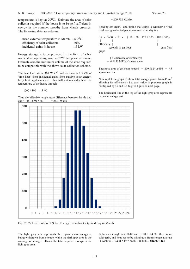
Fig. 23.22 below shows the distribution of solar
radiation for a clear day in March. A house has a heat
requirement of 300 WoC-1, and the internal
N. K. Tovey NBS-M016 Contemporary Issues in Energy and Climate Change 2010 Section 23
114
temperature is kept at 20oC. Estimate the area of solar
collector required if the house is to be self sufficient in
energy in the summer months from March onwards.
The following data are relevant.
mean external temperature in March - 6.9oC
efficiency of solar collectors 40%
incidental gains in house 1.5 kW
Energy storage is to be provided in the form of a hot
water store operating over a 25oC temperature range.
Estimate also the minimum volume of the store required
to be compatible with the above solar collection scheme.
The heat loss rate is 300 WoC-1 and as there is 1.5 kW of
"free heat" from incidental gains from passive solar energy,
body heat appliances etc. this will automatically heat the
temperature of the house through
1500 / 300 = 5 oC
Thus the effective temperature difference between inside and
out = (15 - 6.9) *300 = 2430 Watts
= 209.952 MJ/day
Reading off graph, and noting that curve is symmetric = the
total energy collected per square metre per day is:-
0.4 x 3600 x 2 x ( 10 + 50 + 175 + 325 + 485 + 575)
| | |
efficiency | |
seconds in an hour data from
graph
[ x 2 because of symmetry]
= 4.6656 MJ/day/square meter
Thus total area of collector needed = 209.952/4.6656 = 45
square metres
Now replot the graph to show total energy gained from 45 m2
allowing for efficiency - i.e. each value in previous graph is
multiplied by 45 and 0.4 to give figure on next page.
The horizontal line at the top of the light grey area represents
the mean energy lost.
Fig. 23.22 Distribution of Solar Energy throughout a typical day in March
The light grey area represents the region where energy is
being withdrawn from storage, while the dark grey area is the
recharge of storage. Hence the total required storage is the
light grey area.
Between midnight and 06:00 and 18:00 to 24:00, there is no
solar gain, and heat has to be withdrawn from storage at a rate
of 2430 W = 2430 * 12 * 3600/1000000 = 104.976 MJ

N. K. Tovey NBS-M016 Contemporary Issues in Energy and Climate Change 2010 Section 23
115
In addition there is partial withdrawal from storage between
06:00-07:00, 07:00 - 08:00 and corresponding periods in late
afternoon.
The energy withdrawn in these periods is
2 * [(2430-180)*3600 + (2430-900) *3600)/1000000
| |
6 – 7 am 7 – 8 am
= 27.216 MJ
[the factor 2 is included to account for the afternoon period]
and total energy needed in storage
= 104.976 + 27.216 = 132.192 MJ
Fig. 23.23 Replotted graph showing total energy for whole collector and area where storage is necessary
The same result is obtained if the area of the solar gain
histogram which is above the 2430 line is evaluated.
Each cubic metre of water weighs 1000 kg, and thus the
energy stored per cubic metre per 10C temperature rise is
4.1868 MJ [ this is specific heat of water from data book).
Thus with 25oC temperature range, the volume required =
132.192 / 4,1868 / 25
= 1.26 cubic metres.
================
This example shows the result when the heat loss is steady.
In the case of heating hot water by solar energy, the usage
will be far from constant, but the same basic method may be
applied. Perhaps the easiest way to tackle such a problem is
to start at midnight and work out the cumulative gain over the
day making allowance for use. This represents the net energy
in storage. If the collector area is sized correctly then when
the end of the day is reached there should be no energy
remaining in storage. The maximum positive value of storage
during the day represents the maximum energy to be stored,
and from this the maximum storage volume can be
ascertained.

N. K. Tovey NBS-M106 Contemporary Issues in Energy and Climate Change 2010 Section 24
116
24 WIND ENERGY
24.1 Introduction - theory
Energy from wind is obtained by extracting KINETIC
ENERGY of wind.
K E mV. . 1
2
2
where V is velocity of wind,, and m is mass of air
but mass of air flowing through blades in 1 sec.
= density x area x distance travelled in 1 sec.
= A V
where A is the area swept by the blades,
and is the density of air
Thus K E AV V R V. . . 1
2
1
2
2 2 3 ............ (1)
Equation (1) is the theoretical amount of energy present in the
wind.
HOWEVER, this assumes that all the air is brought to a
standstill, which it can't be otherwise the air would pile up.
The THEORETICAL MAXIMUM POWER which can be
extracted is 59.26% of the KINETIC ENERGY in the wind.
This is also known as the Betz Efficiency, and is a theoretical
limitation on the amount extracted
Practical Efficiencies reduce the amount of power extracted
further.
The best modern aerofoil machines achieve about 75 - 80% of
the THEORETICAL EFFICIENCY - i.e. 40 - 45% overall, but
most rarely exceed 30%. Older machines such as the
American farmstead multi-blade machine usually achieve
efficiencies of less than 20%..
A typical Load Factor for Wind Energy Convertors is 30%,
but often significantly less. Because of poor design and
spacing, the load factor in California is only 20.8%
24.2 Types of Wind Machine - may be classified in three
ways.
i) by type of energy provided.
a) electrical output
b) mechanical output - pumping water etc.
c) heat output - as a wind furnace
- mechanical power is fed to turn a paddle
in bath of oil or water which then heats
up e.g. device near Southampton.
ii) by orientation of axis of machine
a) horizontal axis - HAWT
b) vertical axis - VAWT
iii) by type of force used to turn device
a) lift force machines
b) drag force machines
For electrical output, lift type machines are needed which
have blade tip speeds several times the wind speed. The will
have few blades as multiple blades increase turbulence and
affect the lift. Most turbines are either 2 - or 3 - bladed, but
some early designed had 4 - blades, and a few have just one
blade.
Drag type machines (blade tip speeds are less than the wind
speed) and are more suited to high torque applications such as
water pumping / heating.)
Drag machines have a high solidity - i.e. the amount of the
swept area is high. Typical examples are the multi-bladed
American farmstead water pump and the Savonius rotor.
NOTE: The output from a DRAG type machine would have to
be geared up by a factor of 100 and consequently very large
transmission losses to be suitable for electricity generation.
24.3 Sizes of Machines for different Power outputs.
Output power of machine may be determined from equation
(1).
POWER is proportional to swept area (i.e. square of blade
diameter) and cube of wind speed.
Wind Speed
(m/s)
Blade 5 10 15
diameter (m) (kW) (kW) (kW)
1 0.02 0.16 0.53
2 0.08 0.6 2.1
5 0.49 3.9 13.3
10 1.96 15.7 53
20 7.85 63 212
50 49.1 393 1325
100 196 1571 5301
Output power assumes that overall efficiency of machine is
40% which is typical for latest machines..
Variation in output with height of rotor.
Fig. 24.1 [adapted from Cranfield University WEB site]
showing variation in wind speed. Overall there is a
logarithmic profile to the mean wind speed contour as shown.

N. K. Tovey NBS-M106 Contemporary Issues in Energy and Climate Change 2010 Section 24
117
Fig. 24.2 Zone of affect wind patterns over a wood.
Downwind, there can be significant change in the flow
regime causing differential loading on the turbine.
Above the wind surface there is a boundary layer and the wind
speed, in the absence of minor fluctuations varies in a
logarithmic fashion. Fig. 24.1 shows such variation
superimposed on a logarithmic profile. Thus the higher the
turbine hub, the higher the wind speed, although the variation
becomes less as the height increases. In the first generation
wind turbines in the early – mid 1990s typical hub heights
were 35 – 50m. More recently the norm has been around
70m for a 1.5 MW machine and around 90m for a 2 MW
device.
Variations such as these can place severe differential loading
on the blades and can lead to premature failure from fatigue.
In the 1980s between 5 and 10% of the 10 000 turbines (i.e.
500 - 1000 turbines) of the turbines installed in California
were showing severe signs of fatigue.
It is thus undesirable to site turbines close to areas where
turbulence is likely to be significant - e.g. downwind of an
urban areas or woods.
24,4 Nature of Wind Speed data for Wind Energy
Predictions
Though estimates of wind speed on a 1km x 1km square basis
are available, they are average values over a long period and
can only give approximate estimates of output. The Uk
National Database has mean annual windspeeds at 10m, 25m,
and 45m for each 1km x 1km square across the whole of the
UK. Though such data may be used in initial planning,
ideally, hourly readings over a period of a year are needed at
the development stage of any project.
However, the a serious problem with the data can arise from
the way in which the data is averaged. The following data
shows the mean wind speed as measured on an hourly basis.
The mean wind speed for the 24 hour period is 5.5 metres per
second.
On the other hand the output from a wind turbine depends on
the cube of the wind speed, so more correctly in determining
the effective mean wind speed we should first cubed the wind
speed, determine the mean of the cubes and then take the
cube root. In the example shown, the effective wind speed
now becomes 6.14 metres per second,
When we compare the output using the original figure of 5.5
m/s with the revised figure, there is a difference of just under
40% i.e. the true output is nearly 40% greater than that
determined from the crude mean.
Table 24.1 Example of wind speed variation during day and
two methods used to estimate mean windspead.
Time
Wind
Speed m/s
cube of
Wind
Speed
Time
Wind
Speed
m/s
cube of
Wind
Speed
00:00 3.5 42.9 12:00 8.1 531.4
01:00 4.0 64.0 13:00 8.0 512.0
02:00 4.3 79.5 14:00 7.1 357.9
03:00 4.8 110.6 15:00 6.2 238.3
04:00 5.3 148.9 16:00 5.0 125.0
05:00 5.6 175.6 17:00 4.3 79.5
06:00 6.5 274.6 18:00 4.0 64.0
07:00 7.3 389.0 19:00 3.8 54.9
08:00 8.4 592.7 20:00 3.0 27.0
09:00 8.2 551.4 21:00 2.5 15.6
10:00 8.0 512.0 22:00 3.0 27.0
11:00 8.3 571.8 23:00 2.8 22.0
Frequently data is only available on a daily mean, or even
monthly mean basis, and so estimates based on such values
will often be less than the true resource.
Using the corrected mean speed as indicated above will
improve matters, but it may also over-compensate. Thus
wind turbines for electricity generation cannot operate
below a certain cut-in wind speed - typically around 4.5
- 5 m/s, and secondly, above the design speed the
blades are normally feathered so that the output is at the
designed speed. Finally, in extreme gale force
conditions, the turbines are shut down to prevent
structural damage. Thus a better way to assess the
potential output is to take frequent wind speed
measurements (e.g. hourly or more frequent), and use a
power rating curve to evaluate the actual power output
such as the one shown in Fig. 24.3.
Fig. 24.3 Turbine rating Curve.
Turbines are often classified by their size, and this
refers to their design output. In the example shown in
Fig. 24.3 this would be 300 kW, and this output would
be sustained at any wind speed between 12 and 25 m/s.
Above 25 m/s the turbine would cease to operate and
there would be no output. Similarly below about 3 m/s
0
50
100
150
200
250
300
350
0 5 10 15 20 25 30
Wind Speed (m/s)
Ou
tpu
t P
ow
er
(kw
)

N. K. Tovey NBS-M106 Contemporary Issues in Energy and Climate Change 2010 Section 24
118
there would be no output, whereas at a wind speed of 10
m/s the output would be 228 kW or 76% of the rated
output. Provided that the turbine is reliable then it
should now possible to achieve a load factor of
approaching 30% in the UK, although in some locations
over 40% is achieved on an annual basis. On average,
the figure is around 28%. Turbine rating curves for
different wind turbines may be found at:
http://emd.dk/euwinet/wtg_data/default.asp
although recently (2009) it appears that this link has
changed
24.5 Arrays of Turbines in a Wind Farm
It is easy to estimate the output from a single wind turbine
using the rating curve, but interactions between turbines
occurs when they are clusters in a wind farm. If the wind is
predominantly uni-directional, then they may be sited in rows
at right angles to the wind direction (e.g. the Altmont Pass in
California), but more often the interactive effects must be
considered. Turbulence from one machine can affect
neighbouring ones, and particularly those downwind.
Johansson et al (1993) give a table showing the effects of
clustering .
Table 24.2 Reduction in output arising from Park Effect.
Array Size 5D spacing 7D spacing 9D
spacing
2 x 2 87 93 96
3 x 4 76 87 92
6 x 6 70 83 90
8 x 8 66 81 88
10 x 10 63 79 87
The above table shows the percentage production of wind
power had there been no interference between turbines.
Clearly, less than 7 diameters spacings are unacceptable, and
current wisdom is to use between 7 and 10 diameters as the
norm. In California, many early machines were sited at 1.5 - 3
diameters, and this partly explains the very poor load factors.
One reason why the load factor at Blood hill is inferior to that
at Somerton is because of park effects because of the
proximity of the one turbine to another.
24.6 Examples of Early modern Wind Devices.
A 1.25 MW machine was installed in Vermont in 1941, but
was taken out of service when one of the 7 tonne blades broke
off and flew 1/2 mile. A 60 kW device was installed in UK in
1956 but later abandoned. A 1.25 -kW machine at Tvind in
Denmark was installed in 1958 and provided energy needs for
a School as well as surplus for the neighbouring community. .
In California, and other parts of States (e.g. Hawaii), wind
farms have been established mostly as a result of tax
incentives. Problems with blade fatigue have occurred, and
most have had to have blades renewed. Some turbines have
had a build up of insects on the blades which have caused the
turbines to consume energy rather than generate energy.
Because of the sudden investment, many mistakes were made
and the whole wind energy development nearly collapsed
through people understanding the economic advantages from
tax credits, but had no idea on how to site turbines or how
build ones which operated reliably etc. In the early years
there were many days when large numbers of machines in
California were not operating despite sufficient wind, because
of failure/poor maintenance,
Some very large early machines, although performing very
well, and are economical in both land area and efficiency
suffered from difficulties when failures occured. For
example, on Oahu (Hawaii), just the cost of hiring a large
crane for the week of maintenance during the early 1990s cost
as much as the value of the total output of electricity for a
whole year. On top of that had to be added the cost of the
replacement gear box.
Fig. 24.4 An early 2.5 MW Wind Turbine in Hawaii. The
blade diameter is over 90m.
The largest wind turbines ever built by the mid 1980s was in
the Orkneys on Burgar Hill. This was a 3 MW device with a
blade diameter of just under 100 m
Until 1990 there were few other wind turbines in UK, the
most notable being:-
three in Orkneys including one 3MW device - largest in
world
one 1 MW device at Richborough Power Station,
30 kW machine at Boroughbridge,
one of 150 kW size near Southampton.
odd ones in Cornwall
four of different designs at Carmarthen Bay, including 2
vertical axis machines. [these were blown up by National
Power in 1994]
several 5-15 kW devices, and numerous 50-200W
devices.
In the early 1990s several wind farms were developed, them
ost notable being Delabole in Cornwall, Llandinam in mid-
Wales where there were no fewer than 103 x 300kW devices,
and Blood Hill in Norfolk.
Wind Energy has always been seen as perhaps most effective
renewable source of energy - even CEGB acknowledged this.

N. K. Tovey NBS-M106 Contemporary Issues in Energy and Climate Change 2010 Section 24
119
24.7 Expansion of Wind Power in UK.
During the 1990s, Wind Energy Development was supported in
the UK by a feed in tariff mechanism under the Non Fossil Fuel
Obligation. Since 2002, the support has been via the
Renewable Obligation since when the installation has increased
rapidly reaching 900 MW of new installation last year.
Currently there are a further 1700MW under construction. In
autumn 2008, the Uk overtook Denmark in having the largest
capacity of offshore wind which currently (March 2009) stands
at 565.85MW.
Both the Non Fossil Fuel Obligation and the Renewable
obligation will be covered in the Regulation Module later in the
year. Fig. 24.4 shows the build up of wind capacity over the
last 20 years.
Fig. 24.5 Wind Capacity in the UK to date
Wind Energy
0
2000
4000
6000
8000
10000
12000
14000
16000
18000
1990 1995 2000 2005 2010 2015 2020
Insta
lled
Cap
acit
y (
MW
) offshore in planning
offshore consented
offshore under construction
offshore operational
onshore in planning
onshore consented
onshore under construction
onshore operational
Fig. 24.6 Winbd Capcity in UK and projected capcity. For those under construction it is assumed that they will be fully operational within 2 years of construction start. For those for
which consent has been received, it is asssuemd that only 80% of projects will actually be built and that construction will start in next 2 – 3 years and will be pahsed over 3 years. For
those in planning, it is assumed that only 50% of those currently in the planning system will actually be built’
The first offshore windfarm in UK was at Blyth,
Northumgerland where 2 x 2MW machines are installed. As of
March 2009, 565.8 MW had been installed with a further
774MW under construction. One project, the London Array has
been approved – this wind farm will have a capacity of
1000MW, comparable with that of a fossil fuel power station.

N. K. Tovey NBS-M106 Contemporary Issues in Energy and Climate Change 2010 Section 24
120
The size of offshore wind turbines in increasing and two
turbines both of 5MW capacity have been installed offshore in
North East Scotland (Beatrice). This is a European
Demonstrator Project with the hub height at 88m, and the blade
diameter of 126m.
Details of this project can be seen at the following WEB address
http://www.beatricewind.co.uk/Uploads/Downloads/Scoping_do
c.pdf
Table 24.3 Installed Capacity in Europe (December 2008)
Table 24.4 Offshore Wind Capacity (December 2008).
Installed Capacity Percentage
UK 591 40.2%
Denmark 409 27.8%
Netherlands 247 16.8%
Sweden 133 9.0%
Belgium 30 2.0%
Ireland 25 1.7%
Finland 24 1.6%
Germany 12 0.8%
Currently the largest onshore wind turbine is the 2.75 MW
turbine, named Gulliver, situated at Ness Point in Lowestoft –
see Fig. 24.7).
Fig. 24.7 Largest onshore wind turbine (2.75 MW) in
UK at Ness Point, Lowestoft
24.8 Problems cited regarding Wind Power
1) Visual Intrusion - machines will be large 80+ m high with
blade diameters up to 90m.. Visiual impact is usually at the
heart of all anti-wind lobbies, although they will often try
to cited spurious scientific evidence as a the reason to
object (see below). Visiual impact is a matter of
preference, and anti-wind lobbyists would do better for
their cause if they concentrated on this aspect rather than
the numerous fallacious scientific arguments often claimed
such as:
i) What happens when the wind does not blow?
Currently we have to deal with sudden failures of
large fossil fuel plant – e.g. Sizewell B tripped in
2008 causing the loss of 1188MW within 30 seconds.
This would be equivalent to 40% of our wind turbines
operating under gale force conditions suddenly facing
a calm within 30 seconds – somethigns which
certainly does not occur with the diversity of spread.
In this respect wind generation is far more resilient to
fluctuations than ever conventional generation is.
ii) Noise is a problem. Some people say they are as
noisy as being near a jet engine. It is true that the
noise at the nacelle approaches 100+dB, but the noise
falls off rapidly and at ground level will normally be
below 60dB, a figure which falls off rapidly such that
at around 250m, it will be down to below 40 dB which
is normally taken to be a background rural noise level.
Normally planning authorities will suggest a minimum
of 400m. In any case less than 400m will normally
offshore onshore total
Germany 12 23891 23903
Spain 16740 16740
Italy 0 3736 3736
France 0 3404 3404
UK 591 2650 3241
Denmark 409 2771 3180
Portugal 2862 2862
Netherlands 247 1978 2225
Sweden 133 888 1021
Ireland 25 977 1002
Austria 995 995
Greece 985 985
Poland 472 472
Belgium 30 354 384
Bulgaria 158 158
Czech Republic 150 150
Finland 24 119 143
Hungary 127 127
Estonia 78 78
Lithuania 54 54
Luxembourg 35 35
Latvia 27 27
Romania 10 10
Slovakia 3 3
Cyprus 0 0
Malta 0 0
Slovenia 0 0

N. K. Tovey NBS-M106 Contemporary Issues in Energy and Climate Change 2010 Section 24
121
cause an increase in turbulence and so a developer
would avoid such locations anyway as they would
result in a reduction in output.
iii) TV interference in local region and radio interference
over a larger region, particularly if an array of
machines acts as a long wave radio transmitter - may
affect emergency service frequencies. However, this
can be overcome using suitably located repeater
stations, and is less of a problem nowadays anyway
with the advent of cable and satellite chanels, and
digitial signals are less affected anway compared to
old analogue signals.
iv) Land required for a wind farm of comparable output
of large fossil fuel station is large. While the total
land area is indeed large as machines have to be
spaced 7 – 10 blade diameters apart, apart from a
small hard base at base for cranes and also access
roads, the majority of the intervening land can be
used for agriculture. There are restrictions on
locations of turning the machine off in such
conditions. buildings close to wind turbines for
trubulence effects – see above.
v) Ice on blades causes problems. In the past, ice
formation on tower and blades was a problem, see Fig.
24.8, Ice build up could cause vibration and damage
the blade, or ice could fly off. [It can be shown that
the distance ice may fly from a 330 kW machine can
be as high as 250m]. In modern turbines there are
several strategies which can be adopted, the most
severe being turning the machine off inadverse
conditions. However, in the winter of 2008 – 2009 ice
was seen to come off a wind turbine in East Anglia.
vi) Wind Turbines kill birds. This is an over-rated issue,
and hazards to birds. It is true that in some locations
birds have been killed, but in many locations there is
little evidence. The highest incidence rate is around
3 birds strikes per installed megawatt per year, which
as a worst case scenario would imply around 9000 at
present in the UK. This should be compared with
around 1 million killed each year on the roads and
several million who collide with other fixed
structures. Thus wind turbines have far less impact
on birds than other man made structures or vehicles.
Fig. 24.8 Ice formation on a Wind Turbine
24.9 Economics of Wind Power
The current cost for installation of an onshore wind turbine
varies from around £800 to £1100 per installed kilowatt
depending on the cost of grid connections etc. For offshore
wind, the cost has risen significantly recently as the larger
turbines needed are in short supply at the present time and
exceed £2500 per installed kilowatt.
24.10 Types of Machine - Drag devices.
These devices rely on the drag present by the sails/blades of the
wind device to the wind.
a) VERTICAL AXIS DRAG DEVICES
S - SHAPED ROTOR
Fig. 24.9 A Savonius Rotor
In its simplest form, this device consists of two semi-cylindrical
metal sheets welded together to form an 'S' shape in plan.
The concave side presents a high drag coefficient to the wind
while the convex face has a relatively low drag coefficient. The
device thus rotates.
It is self starting, and produces moderate torque, but the tip
speed is limited to the wind speed. Efficiencies are low -
typically about 10% or less.
APPLICATIONS:- water pumping, wind furnace
A variant of this device separates the two parts of the 'S' - This
is the SAVONIUS MACHINE. Wind deflected by the
windward cup is partly redirected to push the opposing cup.
Efficiencies of this are somewhat improved - up to about 10 -
20%.
PERSIAN "TURNSTILE" DEVICE
In Iran from the 7th century AD walls were constructed across
valleys, and provided with openings with vertical axis devices
shaped like a turnstile. The wind pushed one sail forward while
the opposing sail moving towards the wind was sheltered by the
wall (i.e. its drag coefficient was low). Thus a valley was
dammed to extract wind power in a similar manner to hydro
power.

N. K. Tovey NBS-M106 Contemporary Issues in Energy and Climate Change 2010 Section 24
122
APPLICATION - grinding corn
b) HORIZONTAL AXIS DEVICES - RELYING MOSTLY
ON DRAG
The traditional windmill was of this type with efficiencies up to
10%. The American farm wind multi-bladed device is another
example. Here with careful shaping of the blades efficiencies
up to 30% have been reached, but most devices have
efficiencies nearer 15%.
NOTE: The forces on the blades are proportional to their area,
and so the multi-bladed device has a large starting torque which
makes it ideal for water pumping as it is self starting even
against a pumping load. However, the multiple blades create
substantial eddying and turbulence at high rotor speeds which
limit the efficiency.
Horizontal axis machines must be pointed into the wind to
achieve maximum output. In gale force conditions, they present
very large wind loads on the supporting structure, and The
multi-bladed variety must be feathered by turning the hub axis
at right angles to the wind.
Fig. 24.10 A typical horizontal drag device used for water
pumping in USA.
24.11 Lift Devices
These devices have blades which are carefully shaped into an
aerofoil and rely on lift for operation (see Fig. 24.11).
Fig. 24.11 Representation of forces acting on an aerofoil. The
blade should be viewed as though the observer is above the
wind turbine and looking directly down on a blade which is just
reaching top dead centre.
a) HORIZONTAL AXIS LIFT DEVICES
In these devices, the axis of the machine must be pointed
directly into the wind.
The blades rotate in a plane at right angles to the wind, and the
relative velocity of the wind to the blade is the vectorial sum of
the wind and blade velocity. IT IS THIS RELATIVE
VELOCITY WHICH DETERMINES THE LIFT FORCES ON
THE BLADE.
The blade is tilted at the BLADE ANGLE so that the angle of
attack is optimum. Lift forces are produced by the lower
pressure created on the upper side of the aerofoil and are
directed at right angles to the relative wind direction.
Drag forces are also present from the friction on the blade
surface and this is directed in the direction of the relative wind.
The vectorial sum of the lift and drag forces then determines
whether or not the blade will continue to rotate. Thus if this
relative force vector points in the direction of the blade motion,
the blade will continue to rotate. If the resultant vector points in
the opposite direction, then the blade will stall.
Lift to drag ratios of 50 - 100 are normal with efficiently
designed aerofoils, but this ratio changes with angle of attack,
and above a critical angle, the drag forces increase more rapidly
than the lift forces, and thus stall conditions prevail.
To minimise turbulence and eddy currents, the number of
blades must be kept low, and the starting torque of such
machines is also low. To avoid slow speed stalling, the blade
angles must be constantly adjusted.
Many of these devices are not self starting and need to draw
power from the grid to get them going.
b) VERTICAL AXIS LIFT FORCE MACHINES

N. K. Tovey NBS-M106 Contemporary Issues in Energy and Climate Change 2010 Section 24
123
There are three types here
i) The Darrieus Rotor shaped like a three bladed egg-
beater, [ see front cover for a photograph].,
ii) the straight bladed Darrieus rotor
iii) the Musgrove rotor.
The Darrieus rotor is not self starting, and is very prone to
stalling at slow speeds. The angle of attack of the blades cannot
be adjusted, and the device is not self starting. Some devices
incorporate a small Savonius rotor to start the machine, but this
will limit potential efficiency because of the increased drag they
cause.
The straight sided rotor is really the central part of a Darrieus
rotor, but the pitch of the blades can be constantly varied during
each revolution to optimise performance. Stalling is less of a
problem.
NOTE: frequency of change of blade angle is much higher than
for horizontal axis machines.
The Musgrove rotor has hinged vertical blades which tilt
inwards and this can be used to control speed of device and to
reduce loadings during storm force conditions
Fig. 24.12 A Musgrove Turbine
24.12 Small Scale applications.
The power required by the average household is significantly
larger than that likely to be provided by most small so-called
“micro-wind” generators. The DIY chain B & Q did market
them for installation from 2005, but there have been numerous
problems with them and except when mounted on tower blocks
or individually on their own mast in remote locations they
usually fail to live up to expectations, some falling well short of
the output expected. Of the “mini-wind” turbines – i.e. those
of 6kW or above the load factor is around 10% well below that
of more conventional devices.
Other considerations needed for all wind turbines include:
1) safety switching - to ensure that the grid line is fully
isolated should work need to be done on it,
2) the wind generator is fully protected against lighting
strike surges which might damage the device,
3) considerations of costs paid for electricity exported
to/imported from grid.
The above issues can significantly increase the cost of the
installed devices.
24.13 A worked example for a wind turbine
Fig. 24.13 shows the rating curve for a typical 1500 kW turbine.
Estimate:
i). the annual output if the wind speed profile at the site
during the year is as shown in Table 24.15.
ii). The saving in carbon dioxide emissions resulting from
the operation of the turbine if the carbon dioxide
emission factor for electricity is 0.5 kg / kWh

N. K. Tovey NBS-M106 Contemporary Issues in Energy and Climate Change 2010 Section 24
124
Fig. 24.13 Turbine Rating curve.
Table 24.5 Wind Speed Profile
wind speed (m/s) days
<1 10
1 - 3 20
3 - 5 40
5 - 7 60
7 - 9 100
9 - 11 60
11 - 13 40
13 - 15 15
15 - 17 8
17 - 19 5
19 - 21 3
21 - 23 2
> 23 2
Table 24.5 Wind Speed Profile
The best way to make the estimate is to do the
calculations in tabular form – see Table 24.6
Column 3 is merely the mean of the range of column 1
Column 4 are values read off the gfraph for the relevant
wind speed
Column 5 is the relevant output = i.e. column 2 * column
4 * 24 /1000 – the 24 is to convert to hoursw (from days)
and the 1000 is to give MWh instead of kWH.
Table 24.6 Calculations for Worked Example
Wind
Speed
Number
of Days
Mean
Wind
Speed
Output
kW
Energy
produced
MWh
(1) (2) (3) (4) (5)
<1 10 0 0 0
1 - 3 20 2 0 0
3 - 5 40 4 0 0
5 - 7 60 6 90 129.6
7 - 9 100 8 680 1632
9 - 11 60 10 1275 1836
11 - 13 40 12 1500 1440
13 - 15 15 14 1500 540
15 - 17 8 16 1500 288
17 - 19 5 18 1500 180
19 - 21 3 20 1500 108
21 - 23 2 22 1500 72
> 23 2 24 0 0
TOTAL 6225.6
As the total output is 6225.6 MWh and 0.5 tonnes of carbon
dioxide are4 displaced for each MWh generated the total carbon
dioxide saved will be 6225.6 * 0.5
= 3112.8 tonnes
In other situations, the frequency of the wind speed may be
given instead of the number of days
Thus table 24.7 shows the exactly same data as in Table 24.5
but this time as percentages

N. K. Tovey NBS-M106 Contemporary Issues in Energy and Climate Change 2010 Section 24
125
Table 24.7 Wind Speed Profile shown as a percentage
wind speed (m/s) frequency
<1 2.74%
1 - 3 5.48%
3 - 5 10.96%
5 - 7 16.44%
7 - 9 27.40%
9 - 11 16.44%
11 - 13 10.96%
13 - 15 4.11%
15 - 17 2.19%
17 - 19 1.37%
19 - 21 0.82%
21 - 23 0.55%
> 23 0.55%
Once again it is most efficient top proceed in tabuilar form –
Table 24.8
Table 24.8 – Worked example when windspeed
information is given as a frequenct
Wind
Speed
Mean Wind
Speed frequency
Outpu
t kW
Power *
frequency
(1) (2) (3) (4) (5)
<1 0 2.74% 0 0
1 - 3 2 5.48% 0 0
3 - 5 4 10.96% 0 0
5 - 7 6 16.44% 90 15
7 - 9 8 27.40% 680 186
9 - 11 10 16.44% 1275 210
11 - 13 12 10.96% 1500 164
13 - 15 14 4.11% 1500 62
15 - 17 16 2.19% 1500 33
17 - 19 18 1.37% 1500 21
19 - 21 20 0.82% 1500 12
21 - 23 22 0.55% 1500 8
> 23 24 0.55% 0 0
TOTAL 711
In this approach column 5 is merely the product of the output
(from column 4) and the frequency as a fraction. There is no
need to multiply by 24 as in previous method. The sum of
column (5) then gives the effective average output for the
turbine, i.e. 711 kW. This implies that the load factor is
711/1500 = 47.4% which is on the high side, but possible.
To work out the total amount of energy produced multiply this
figure of 711 by the number of hours in a years (i.e. 8760)
= 711 * 8760 /1000 = 6225.6 MWh – i.e. exactly the
same as before
Note the division by 1000 is to convert from kWh to MWh.
24.14 The Future of Wind
The UK has the best wind resource in Europe and load factors
significantly in excess of those being achieved in Germany are
now common. In 2008 just under 1000 MW of new wind
installation was completed and as this is the only technology
which is currently available (other than biomass) which is
technically mature and also potentially economically attractive,
this will be key in reaching the target of 15% of all energy
consumption to come from renewable by 2020. Indeed since
non-electricity uses are likely to fall well short, the electricity
target isw likely to be set at over 30% which will in trun imply
the installation of at least a further 10000 MW of wind
generation by 2020, or over 3 times the current installed
capacity.

N. K. Tovey NBS-M016 Contemporary Issues in Energy and Climate Change 2010 Section 25
126
25. Tidal Power
Churchill No 2 Barrier, Orkney. This barrier is 620 m long and was constructed during World War II. There is a difference in tides of 1 hour 40 minutes between the east and west
sides of the barrier giving the potential for a tidal barrage without much of the capital costs associated with construction and without most of the environmental problems associated
with such barrages.
25.1 Tidal Power - Theory
Tides arise from the rotational motion of the earth and the
differential gravitational field set up by the Earth,
Moon, and Sun. The relative motions of these cause
several different tidal cycles:-
1) a semi-diurnal cycle - period 12 hrs 25 mins
2) a semi-monthly cycle - (i.e. Spring - Neap
Tides) corresponding with the position of the
moon
3) a semi-annual cycle - period about 178 days
which is associated with the inclination of the
Moon's orbit. This causes the highest the
highest Spring Tides to occur in March and
September.
4) Other long term cycles - eg a nineteen year
cycle of the Moon.
The Spring Tides have a range about twice that of neap tides,
while the other cycles can cause further variations of up to 15%.
The Tidal range is amplified in estuaries, and in some
situations, the shape of the estuary is such that near resonance
occurs. This happens in the Severn Estuary where a tidal range
at Cardiff is over twice that at the mouth of the estuary (see
diagram on separate sheet).
A barrage placed across such an estuary can affect the resonance
conditions, and either enhance further the potential range or
suppress it. Careful modelling is therefore needed in the
evaluation of any scheme.
Potential power is proportional to area impounded and the
square of the tidal range. Thus about 4 times as much power
can be generated at spring tides as at neap tides.
Historically most interest has been shown in Tidal Basin
Schemes although in the last few years ineterst has also been
shown into marine current deivces which operate in a similar
manner to Wind Turbines. Such devices are described in
section 25.7. There have also been ideas suggested for Tidal
Lagoons which are in essence a derivative of the basin schemes.
(section 25.8).
25.2 Tidal Power - Introduction to Basin Schemes

N. K. Tovey NBS-M016 Contemporary Issues in Energy and Climate Change 2010 Section 25
127
There have been tidal mills in operation for many centuries e.g.
at Woodbridge in Suffolk, but only in the last 25 years have
major new schemes been constructed to generate electricity.
Examples include the 240 MW Tidal Power Station at La Rance
near St Malo in France, a scheme in northern USSR, and more
recent schemes in China. All except La Rance are small
schemes < 10 MW.
As early as 1925, consideration for a tidal barrage across the
Severn Estuary was given by the Brabazon Committee. The
proposal was for a barrage just seawards of the present Severn
Bridge.
Subsequent schemes have favoured a more seaward barrage
some as far seaward as Minehead.
Three Energy Papers on Tidal power have been written (Nos.
23, 27, and 46). The last of these is the so called Bondi Report
(1981). There are also references to Tidal Power in the more
recent Energy Papers 55 - 66.
Other estuaries in the UK under consideration include:-
1) Solway Firth
2) Morecombe Bay
3) The Wash
4) Humber
5) Dee
6) Mersey (recently this scheme has been promoted actively
and could be the first scheme in the UK).
7) Strangford Lough
The total potential, if all sites were developed, would be to
generate about 125 PJ of electricity per year, or about 16% of
UK consumption.
About 147 PJ per annum (6%) could be generated by the
favoured scheme for the Severn which has the second highest
tidal range in the world (after the Bay of Fundy in Canada).
Tidal Basin Schmes fall into one of 5 categories.
1) schemes working on EBB flow only
2) schemes working on FLOOD flow only
3) schemes working on both EBB and FLOOD
4) Double Basin Schemes
5) Any of the the above schemes but incorporating pumping at
high or low tide.
25.2.1 EBB schemes
Generation on EBB flow only ( see Fig. 25.1) . The basin
fills through sluice gates which are closed at high tide, and
the water allowed to pass through the turbines as the tide
ebbs.
Generation starts around 4 hours after high tide to ensure
the head is large, and hence the output is greatest.
Generation can be continued for up to 2 hours after low tide.
Generation is possible for only one-third of time.
The water in the basin is always above mean sea level, and
thus the mean water level in the basin is raised compared to
conditions before the barrage is constructed..
Fig. 25.1 Generation from Tidal Power in the EBB Mode
25.2.2 FLOOD Schemes
Generation on FLOOD flow only. (Fig. 25.2) The basin is
emptied rapidly through sluice gates which are then closed at
low tide. Generation occurs as water flows in to flood the
basin.
As with ebb flow schemes, generation is restricted to 4 hours
in every 12 (2 hours either side of high tide).
The total energy generated would be less as less water would
be able to pass through the turbines.
The mean water level in the basin would be below mean sea
level, and hence would cause a hazard to shipping.
25.2.3 Two Way Generation Schemes
Two way generation on both EBB and FLOOD. This is a
combination of the above methods (Fig. 25.3).
Generation is possible for more than 8 hours in any 12 hour
cycle.
However, the total energy output is reduced as the mean
height of the basin is at about mean sea level, and the
effective head during generation is reduced. Also two way
turbines are inherently less efficient.
Ports need relatively high water levels for shipping for at
least part of the time and if, as with the Svern Barrage, there
are several such ports, these would probably suffer.
The cost would be up to 20% greater than the equivalent
single flow scheme.
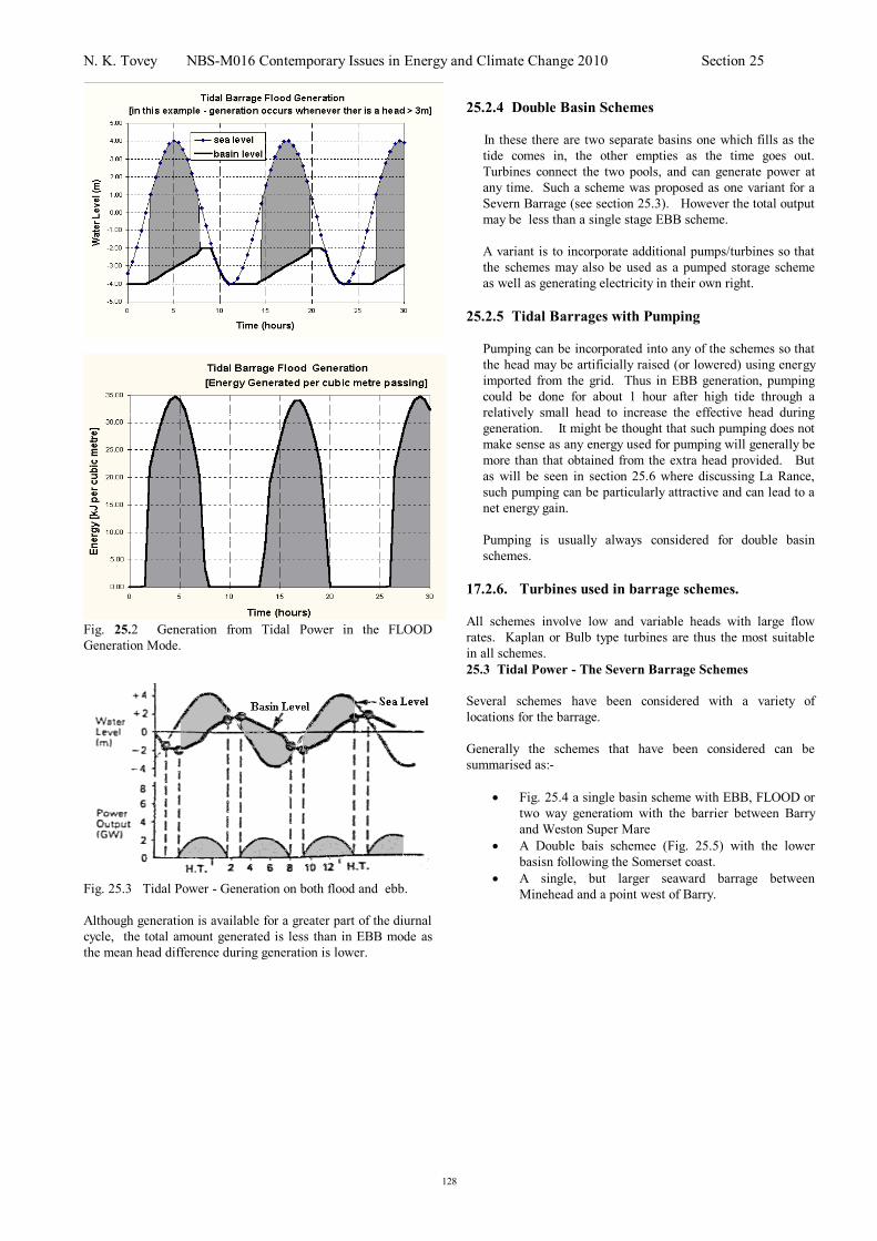
N. K. Tovey NBS-M016 Contemporary Issues in Energy and Climate Change 2010 Section 25
128
Fig. 25.2 Generation from Tidal Power in the FLOOD
Generation Mode.
Fig. 25.3 Tidal Power - Generation on both flood and ebb.
Although generation is available for a greater part of the diurnal
cycle, the total amount generated is less than in EBB mode as
the mean head difference during generation is lower.
25.2.4 Double Basin Schemes
In these there are two separate basins one which fills as the
tide comes in, the other empties as the time goes out.
Turbines connect the two pools, and can generate power at
any time. Such a scheme was proposed as one variant for a
Severn Barrage (see section 25.3). However the total output
may be less than a single stage EBB scheme.
A variant is to incorporate additional pumps/turbines so that
the schemes may also be used as a pumped storage scheme
as well as generating electricity in their own right.
25.2.5 Tidal Barrages with Pumping
Pumping can be incorporated into any of the schemes so that
the head may be artificially raised (or lowered) using energy
imported from the grid. Thus in EBB generation, pumping
could be done for about 1 hour after high tide through a
relatively small head to increase the effective head during
generation. It might be thought that such pumping does not
make sense as any energy used for pumping will generally be
more than that obtained from the extra head provided. But
as will be seen in section 25.6 where discussing La Rance,
such pumping can be particularly attractive and can lead to a
net energy gain.
Pumping is usually always considered for double basin
schemes.
17.2.6. Turbines used in barrage schemes.
All schemes involve low and variable heads with large flow
rates. Kaplan or Bulb type turbines are thus the most suitable
in all schemes.
25.3 Tidal Power - The Severn Barrage Schemes
Several schemes have been considered with a variety of
locations for the barrage.
Generally the schemes that have been considered can be
summarised as:-
Fig. 25.4 a single basin scheme with EBB, FLOOD or
two way generatiom with the barrier between Barry
and Weston Super Mare
A Double bais schemee (Fig. 25.5) with the lower
basisn following the Somerset coast.
A single, but larger seaward barrage between
Minehead and a point west of Barry.

N. K. Tovey NBS-M016 Contemporary Issues in Energy and Climate Change 2010 Section 25
129
Fig. 25.4 A proposed single basin scheme
Fig. 25.5 A proposed double basin scheme. The upper basin would be filled at high tide, the lower one emptied at low tide.
Fig. 25.6 A proposed single basis scheme. This is largest of all and would generate about 12000 MW.
After an extensive review, the Bondi Committee considered
that the EBB only schemes without pumped storage were the
most cost effective, and proposed three schemes:-
a) A seaward barrage near Minehead which would have
an installed capacity of 12000 MW (i.e. 24% of
current installed capacity, and would generated about
9% of the needs of England and Wales (Fig. 25.6).
b) An inner barrage just seaward of Cardiff which would
have an installed capacity of 7200 MW (Fig. 25.4).
c) A staged scheme involving scheme (b) with the option
to provide a second basin on the southern side of the
estuary between Weston super Mare and Minehead.
The Bondi Committee favoured scheme (b).
Tidal Power from the Severn is predictable (unlike other
renewables). However, there will be many occasions when the
peak demand will occur when no power is available.
In the Bondi committee report it was estimated that an installed
capacity of 7.2GW would only reduce the requirement for new
fossil fuel / nuclear plant by about 1 GW because these plant
would still be required to meet peak demand. Exepreince of La
Rance scheme indicates that Load Factors of around 25% can be
achieved – cf 20 – 40% for Wind turbines, depending on
location. Tidal barrage schemes will save fossil fuel and
reduce carbon emissions, but will not significantly reduce
capacity requirement for new conventional stations unless
pumped storage is incorporated [NKT’s comment]..
25.4 Tidal Power - Some Environmental Considerations of
Basin Schems.

N. K. Tovey NBS-M016 Contemporary Issues in Energy and Climate Change 2010 Section 25
130
There are several effects which such a scheme would have
including:-
1) accessibility of shipping to existing Ports
2) employment - the Severn Barrage would provide
jobs for about 21000 for up to 10 years.
3) large quantities of concrete will be needed and the
materials for this and the earth fill barrage will
have to be shipped to site.
4) water quality in the estuary might be affected if
pollutants are not dispersed so readily.
5) recreation facilities could be provided in the basin.
6) extra pumping would be needed for land drainage.
7) sea defences would be less vulnerable to attack.
8) reduced sediment transport might lead to siltation
behind barrage - however, by allowing flushing
during summer (or periods of low demand), much
of the impact of this can be reduced more easily
than for hydro schemes,.
9) some species of birds would decline (especially
wading birds), but other species would probably
increase. However, with the double basin scheme
it is likely that the habitat for wading birds would
increase.
25.5 Tidal Power - other considerations of basin schemes.
EBB generation tidal schemes would NOT increase the
requirement for pumped storage schemes unless there is a high
proportion of nuclear plant or if the proportion of fossil fired
stations is low, or the proportion of other renewables is high.
Fossil fired plant would be used to provide firm power at times
of demand with no tidal power available. However, if these
stations are displaced by large numbers of other renewable
resources, then the need for extra storage would increase.
During the 1980s, the CEGB were interested in Private money
being spent on Tidal Schemes as large sums of money would be
required - four times the capital cost of Sizewell. However, the
former CEGB would NOT give a guarantee that they will
purchase all or even ANY of the power at a fixed price. This
makes the economics difficult to evaluate. In the new regime
following privatisation, it would be even more difficult to
guarantee a a purchase price unless there was legislation.
The National Grid would argue that once sources of power are
available (i.e. stations constructed) the decision to use power
from that source is based solely on the marginal costs (including
any subsidy (e.g. NFFO), and not the capital costs. Unless there
is an agreed price (as there was originally for wind under
NFFO) the viability for tidal is less certain if large schemes go
ahead. On other hand smaller schemes such as the Mersey
might well be more viable.
Double basin schemes have an advantage in that they can
enhance the storage opportunity through additional pumped
storage. This aspect is not taken into account in financial
considerations. Since extensive renewable energy development
would necessarily lead to an increase demand for pumped
storage, such an additional facility could be an added benefit
and should be treated as a net economic benefit for the whole
Electricity Supply System. This needs central coordination
and planning to achieve..
If a double basin scheme were built, there could be further
advantages by combining wind turbine generation at the site
with generation as an integrated package, rather than allowing
renewables to compete one with another.
25.6 La Rance scheme
The "La Rance Tidal Barrage" is situated a few kilometres
upstream from St Malo at a location where the tidal range is
13.5m during Spring Tides. The enclosed basin has an area of
2200 hectares and the barrage was completed in the late 1960s.
the barrage itself is 750m long and the foundations are 13 m
below mean French Ordnance Datum. The barrage
incorporates shipping locks and provides a dual carriageway
link between St Malo and Dinard.
There are 24 units each with a maximum generation of 10 MW
generating at 3500 volts which is stepped up to 225 kV for the
French SuperGrid. The turbines are 4-bladed Kaplan Bulb
turbines with a diameter of 5.35 m with output as follows.
TABLE 25.1 Output Power per unit for different head
differences at La Rance.
Head
> 9m 7m 5m 3m
Ebb Flow 10 10 8 3.2
Flood Flow 10 9.5 5.5 2
The generation is thus greatest in the EBB generation mode.
The barrage can operate in a one way mode, although EBB flow
generation is only normally considered, or on two way flow.
Overall, the output in recent years indicates a load factor of
around 25%, which is higher than the 16 - 17% several text
book imply.
In one way operation the sluice gates are opened on the
incoming tide to fill the basin and then closed at high tide. As
the tidal cycle is sinusoidal, the fall in level from high tide is
relatively small in the first 3 hours, and no generation takes
place. Generation will continue beyond low water as the head
will still be sufficient for generation for up to 90 minutes after
low water (Fig. 18.7).
A variant of the scheme is to pump water for a period of about 1
hour after high water into the basin. Though this introduces
inefficiency (~85% efficient) the head difference is small and
generation can later take place over a greater head and hence
this pumping arrangement is a net energy producer. Electricity
for pumping is drawn from the grid, and clearly if this coincides
with peak demand, no pumping will be done on that tidal cycle
(Fig. 25.7).
The Two way operation which is used from time to time starts
with the basin emptied with the sluice gates closed. When the
tide has risen sufficiently (usually about 4 hours after low water,
generation in the flood mode can occur for up to 1.75 hours.
The turbines are stopped and the sluice gates opened to allow
the basin to fill - with pumping if relevant. The sluice gates
are closed at high tide, and generation on the Ebb tide then
takes place as before except that generations ceases at low tie to
allow the sluice gates to be opened to empty the basin. In
theory pumping to empty the basin is possible, but cavitation
problems may prevent this as the turbines must always be
completely covered with water. The cycle then resumes.

N. K. Tovey NBS-M016 Contemporary Issues in Energy and Climate Change 2010 Section 25
131
Fig. 25.7 One way operation of La Rance – incorporating
optional pumping. Additional output can be obtained by
overfilling basin at high tide. The head difference during
pumping is less than that in generation, and hence there is a net
gain in the system.
In two way operation, the basin does not rise to the same level
as in single way operation as the turbines form a restriction to
the incoming tide. As a result, the two way generation usually
provides less electricity, but the generation period is more
uniformly spread over the diurnal cycle. Assume that the tidal
cycle is exactly 12 hours.
25.7 Marine Current Devices
There are several regions around the coast of the UK where
significant currents exists. Often these occur in narrow
straits between islands – e.g. Eynhallow Sound between
Mainland Orkney and Rousay, in the Fall of Warness near
Eday (Orkney), the Pentland Firth, and between Cap de la
Hague and Aldernay. Barrages are costly to build and
several people believe they are environmentally undesirable.
It is possible, in theory to construct marine current turbines
which are like underwater wind turbines to harness power
from the currents. Typical sizes will be 0.5 – 2MW and
individual or clusters of devices can be installed. The
strong currents and corrosion do mean that technical
developments are still needed and the technology is
probably 20 years + behind that of wind. A single
demosntration scheme of 750 kW has been operating off
Cornwall. The EMEC Centre in Orkney has a test site at
the Fall of Warness, and it is hoped to fully commission this
in mid – late 2007 with direct Grid connection. These are
experimental and if successful, and if the costs could be
brought down, then full scale commercial exploitation
might be possible in around 10 years time or so.
. The formula to get the power from a marine turbine will be
exactly the same as for a wind turbine:-
where is the efficiency (typically around 40% for the best
machines)
is the density of sea water which may be taken as
1070 kg m-3
R is the radius of the area swept
V is the wind velocity.
Typically the diameter of the blades should not be more than
50% of the water depth and it makes sense to have all turbines
in an area of the same diameter. That means the size will be
dictated by the minimum depth of water where the turbines are
to be installed. The density of sea water is nearly 1000 times
that of air, and so even though the velocity is much less,
significant output is potentially obtainable from devices with
blade diameters from about 10 m upwards. For a 0.5 MW
device a blade diameter of around 20m is required in a current
of 2 m s-1, whereas for a windturbine of equivalent output a 40
m blade diameter with a wind speed of 12 m s-1 is required.
Because the current speeds are relatively low (in normal
generation terms), it would not make sense to attempt to
generated in synchronism with the mains. Instead
consideration is likely to be given to generating with DC and
then inverting to AC when the power comes ashore.
Marine Current Turbines will have to work in a harsh
environment and technical problems such as offshore and
underwater maintenance still need to be addressed.
25.8 Tidal Lagoons.
A relatively recent development in Tidal Power has been the
development of the Tidal Lagoon principle. Unlike the Tidal
barrage, for which there is already a full scale operational
device at La Rance, and several individual tidal stream devices,
there is no operating Tidal Lagoon scheme. Whi8le the Tidal
Lagoon does offer a considerable potential it has yet to be
tested, and unlike the tidal stream devices which can be
constructed in modular form, the lagoon requires the
construction of very large devices which will not only be a long
time in construction, but also have significant initial
investments in embodied energy and associate carbon in the
construction phase. While in the long term there will be a
significant saving tin carbon, the initial heavy carbon outlay is
an issue which must be addressed, and may require a significant
phasing (and consequential limit on the rate of deployment) of
such schemes if there is not to be a significant increase and
overshoot in carbon emissions in the criticval period between
now ond 2025.
A tidal lagoon requires the construction of a large barrier to
enclose a large tidal area. Unlike a barrage this is not connected
to land, and is located in relatively shallow areas in tidal
esturaries such as in Swansea Bay in the Severn Esturary.
A barrier some 90 miles long would be constructed with the
requirement of some 200 million tonnes of aggregate. This
would create an artifical basin from which both flood and ebb
generation is possible (probably supported by pumping).
It is probable that the lagoon wmight be built in stages, but
until a complete section is isolated from the main estuary, no
generation can take place and this is a disadvantage compared to
tidal stream edevices. A normal tidal barrage would require
only around 7 – 10% of the amount of aggregate, and this should
be somewhat quicker to construct and start recover the benefits.
It is claimed that a laod factor of 61% might be achieved, which
is high for renewable generation, although experience with other
technologies suggests that such levels are unlikely to be
achieved in the early schemes. However, if it does then there
could be significant advantages.
Perhaps the best aspects of such lagoons is, like the double
basin scheme for barriers the potential ability to provide a level
of pumped storage, particularly if multiple basins schemes are
used.
32
2
1VR

N. K. Tovey NBS-M016 Contemporary Issues in Energy and Climate Change 2010 Section 25
132
25.10 Consultation on Severn Tidal Schemes January –
April 2009
In January 2009, the new Department of Energy and Climate
Change launched an extensive public consultation relating to
several different proposed schemes for extracting energy from
the tides in the Severn Estuary. The consultation may be
consulated at:
http://severntidalpowerconsultation.decc.gov.uk/
Essentially there are 5 separate barrage schemes, several
lagoons, some of which are connected to land, and two tidal
fence schemes. These are summarised in the following:
Fig. 25.8 Proposed Barrier schemes in the 2009 consultation

N. K. Tovey NBS-M016 Contemporary Issues in Energy and Climate Change 2010 Section 25
133
Fig. 25.9 Proposed Lagoon schemes in the 2009 consultation
Fig. 7.10 Proposed Tidal Fence Schemes in the 2009 consultations.

N. K. Tovey NBS-M016 Contemporary Issues in Energy and Climate Change 2010 Section 25
134
Comparison of different schmes
Installed
capacity
Annual
Generation
Earliest
operation
capital
cost Cost per unit
MW TWh £bn p/kWh
B1 Outer Barrage from Minehead to Aberthaw 14800 25.3 2022 29 7.3
B2 Middle Barrage from Hinkley to Lavernock Point ~9950 19.3 2021 21.9 7.82
B3 Middle Barrage ( Cardiff - Weston ) 8640 16.8 2020 18.3 7.39
B4 Inner Barrage (Shoots Barrage) 1050 2.77 2019 2.6 6.69
B5 Beachley Barrage 625 1.59 2018 1.8 8.21
F1a Tidal Fence (Cardiff - Weston) 0.7 ?
4.4 40.47
F1b Tidal Fence (Minehead -Aberthaw) 3.3 6.3 14.33
L3a English Grounds Tidal Lagoon 1.41 2018 3.1 11.35
L3b Welsh Grounds Tidal Lagoon 1360 2.31 2019 2.6 11.27
L3c Peterstone Flats 1120 2.33 2019 3.3 9.03
L3d Bridgewater Bay 1360 2.64 2020 3 8.29
L3e(i) Offshore Tidal Lagoon 1 1360 2.6 2020 5.8 12.86
L3e(ii) Offshore Tidal Lagoon 2 760 1.32 2019 3.5 15.05
• Tidal Fences are unknown technology so uncertainty over operation date.
• For comparison Sizewell B generates ~8.0 TWh per annum.
• Data do not consider potential advantages of double barrier scheme with pumped storage – something which will be needed
with more renewables
NOTES:
• In 1979, construction of Dinorwig Pumped Storage Power station (1800 MW) was started and cost £0.45bn
• Compared to January 1979, the RPI in Jan 2009 was 399.89, i.e. prices were 4 times those in 1979. Thus the cost of similar
station today would be £1.8bn or £1m per installed MW.
• If 50% of capacity were available as pumped storage, the Minehead – Aberthaw basin if made a double basin would provide
same capabilities as spending £7bn elsewhere on alternative pumped storage and is thus a net benefit to the scheme.
• Such additional spending will be needed in future with increased renewable generation such as wind
• A holistic approach is needed
See http://www.independent.co.uk/opinion/letters/letters-tidal-power-1517932.html
• Public Consultation on Severn Tidal Schemes is currently open – until 23rd April 2009.
•
• Have your say!
• See http://severntidalpowerconsultation.decc.gov.uk/ Where more details of schemes may be found
25.10 Numeric Example of a Tidal Barriers.
The following are two numeric examples of how an assessment
of tidal energy may be made. On the Energy Field Courses in
1999 and 2001 estimates were made of the potential of the Race
of Aldernay between Cap de la Hague and Aldernay, while in
2005, and 2007, barrier and tidal streams in Orkney wefre
examined.
25.11 Example of an existing Tidal Barrage where there is a
tide height difference – e.g. Churchill Barriers, Orkney.
A man made causeway is built joining two islands. After
construction it is found that there high tide on the east is 3
hours before high tide on the west.
The tidal heights are shown in the following table and graph
Time relative to
east side (hrs)
Height on east
side (m)
Height on west
side (mj)
0 1.80 0.00
1 1.56 0.90
2 0.90 1.56
3 0.00 1.80
4 -0.90 1.56
5 -1.56 0.90
6 -1.80 0.00
7 -1.56 -0.90
8 -0.90 -1.56
9 0.00 -1.80
10 0.90 -1.56
11 1.56 -0.90
12 1.80 0.00
13 1.56 0.90

N. K. Tovey NBS-M016 Contemporary Issues in Energy and Climate Change 2010 Section 25
135
. The shaded area shows the output for each cubic metre
flowing through the turbine [ thisshaded area is shown for
information only]..
Estimate the daily electricity production and the mean power
produced if a turbine with a diameter of 4047mm is inserted
into the causeway. Power can be extracted whenever the height
difference between the two sides of the barrier exceeds 0.9mThe
density of sea water is 1070 kg m-3, and the efficiency of the
turbines is 80%.
First work out the height difference in column 4 and then the
effective height in column 5. Whenever the height is less than
the critical 0.9m there is no generation available. The shaded
columns are direct copies from the data. Notice the data are
symmetric and many values are the same value (or same value
but opposite sign)
Time relative to east
Height east
Height west
Height differ-ence
Effective
Height
Velocity Cube of velocity
(m) (m) (m) (m) (m/s)
0 1.80 0.00 1.80 1.80 5.94 209.87
1 1.56 0.90 0.66 0.00 0.00 0.00
2 0.90 1.56 -0.66 0.00 0.00 0.00
3 0.00 1.80 -1.80 -1.80 5.94 209.87
4 -0.90 1.56 -2.46 -2.46 6.95 335.08
5 -1.56 0.90 -2.46 -2.46 6.95 335.08
6 -1.80 0.00 -1.80 -1.80 5.94 209.87
7 -1.56 -0.90 -0.66 0.00 0.00 0.00
8 -0.90 -1.56 0.66 0.00 0.00 0.00
9 0.00 -1.80 1.80 1.80 5.94 209.87
10 0.90 -1.56 2.46 2.46 6.95 335.08
11 1.56 -0.90 2.46 2.46 6.95 335.08
12 1.80 0.00 1.80 1.80 5.94 209.87
2179.8
Now water flowing through turbine, must be consistent.
i.e potential energy of head difference = kinetic energy flowing
thorugh turbines
i.e. mgh = 0.5 m V2
or V = sqrt( 2 g h)
where g is the acceleration due to gravity = 9.81 m s-1
Hence enter the values of velocity as computed in the
manner outlined above in column 6. Notice you should
disregard the –ve sign in these calculation as this merely
implies two way flow. This will be the velocity of the water
through the turbine.
Now by continuity
the mass passing per second = density x volume
= density x velocity x cross section area
= V R2
and kinetic energy = 0.5 m V2 multiplied by efficiency
so energy available = 0.5 V R2
V2 = 0.5 R
2 V
3
substituting values for , , and R
gives the theoretical energy at any instant = 5505.09 V3
(remember that density of SEA water is 1070 kg m-3
).
Alternatively the energy available in a day will be
2 x 5505.09 x V3
[the factor 2 comes from two tidal cycles per day)
Thus to find total energy work out V3 and enter values in
column 7 and sum
total energy will thus be 2 * 5505.1 *2179.8 /1000/1000
MWh per day.
= 24.00 MWh per day
and the rated output of the turbine will be 24.00/24 = 1MW
25.12 Enclosed basin Tidal Power Example (La Rance):
The height (h) of the water level above mean sea level in the
Rance Estuary in Northern France may be approximately found
from the relationship:-
h dt
p 0 5
360. cos( )
where t is the time in hours after high tide,
d is the range (maximum-minimum) of the tide = 9m,
and p is the period between high tides (12.5 hours in this
case).
Generation of electricity takes place whenever there is a head
difference of 2.089m or more, and continues until the level of
water in the basin falls to 0.779m below mean sea level. The
turbines have an efficiency of 60%. You may assume that the
density of water is 1000 kg/m3.
Estimate how long generation can continue during each tidal
cycle. Estimate also the mean output from the power station if a
total of 108.73 x 10⁶ m3 of water pass through the turbines
during generation.
SOLUTION:
First use the equation to work out the height of the tide at each
hour from 0 up to 12.5 hours. It is only necessary to do this
once an hour:

N. K. Tovey NBS-M016 Contemporary Issues in Energy and Climate Change 2010 Section 25
136
HOUR HEIGHT (m) HOUR HEIGHT (m)
0 4.500 7 -4.184
1 3.943 9 -0.843
2 2.411 10 1.391
3 0.283 11 3.280
4 -1.916 12 4.359
5 -3.641 13 4.359
6 -4.465
Now plot a graph with the time as the x-axis.
Now draw on lines which are 2.089m below high tide
(representing start of generation), and 0.779m below mean tide
(representing the end of generation.
The start coincides exactly with the 2 hour point. This can be
checked as at two hours the difference from high tide is 4.5 -
2.411 = 2.089m).
Similarly the generation ceases when the level is 0.779m below
mean tide, but the head of 2.089 must still be maintained. So
the level of the tide when generation ceases will be:-
-0.779 - 2.089 = - 2.868 i.e. exactly the
height after 8 hours.
So generation will occur for 8 - 2 = 6 hours (answer to first
part).
======
There are now two ways to proceed for the second part:-
Method 1: Graphical Method
Plot on the basin level assuming a linear decline from the start
to the end of generation.
Then measure off at each hour the height difference between the
basin level and the tide as shown in the following table:-
HOUR HEIGHT HEAD
0 4.500 no generation
1 3.943 no generation
2 2.411 2.089
3 0.283 3.337
4 -1.916 4.656
5 -3.641 5.502
6 -4.465 5.446
7 -4.184 4.285
8 -2.868 2.089
9 -0.843 no generation
10 1.391 no generation
11 3.280 no generation
12 4.359 no generation
13 4.359 no generation
This method continues after the Numeric Method
NUMERIC METHOD
It is not difficult to linearly interpolate to get the height of the
basin at any hour between the start and end of generation as
shown in the table below. Once this has been found it is a
simple matter to subtract the tide level from the basin level to
get the effective head.

N. K. Tovey NBS-M016 Contemporary Issues in Energy and Climate Change 2010 Section 25
137
HOUR HEIGHT BASIN HEAD
0 4.500 4.500 no generation
1 3.943 4.500 no generation
2 2.411 2.089 2.089
3 0.283 3.620 3.337
4 -1.916 2.740 4.656
5 -3.641 1.861 5.502
6 -4.465 0.981 5.446
7 -4.184 0.101 4.285
8 -2.868 -0.779 2.089
9 -0.843 no generation
10 1.391 no generation
11 3.280 no generation
12 4.359 no generation
13 4.359 no generation
BOTH METHODS
The figures in the final columns for both methods are the same.
The energy generated at any one instant is ...... m.g.h
To find out the MEAN OUTPUT we need to find the mean head
over the period.
There is a small catch here:-
For the shaded area we can take the approximation that the head
is that for 5 hours, similarly for 4 hours and 6 hours etc. But
for both 2 hours and 8 hours, the generation is for only half the
time, so the mean generation height is given by:-
0.5 x 2.089 + 3.337 + 4.656 + 5.502 + 5.446 + 4.285 + 0.5 x 2.089
---------------------------------------------------------------------------
6
= 4.219 m
The time interval is 6 x 3600 seconds
volume density of water
| |
So mean output = 108.73 x 106 x 1000 x 9.81 x 4.219
------------------------------------------
6 x 3600
= 125 MW
=======
So mean output is 125 MW