NBER WORKING PAPER SERIES

TRADE INTEGRATION AND RISK SHARING

Aart Kraay

Jaume Ventura

Working Paper 8804

http://www.nber.org/papers/w8804

NATIONAL BUREAU OF ECONOMIC RESEARCH

1050 Massachusetts Avenue

Cambridge, MA 02138

February 2002

We thank Pol Antràs, Antonio Fatás, Philip Lane and participants in the International Seminar on

Macroeconomics at University College Dublin, June 2001, for their useful comments. The views expressed

herein are those of the authors and not necessarily those of the National Bureau of Economic Research or

The World Bank.

© 2002 by Aart Kraay and Jaume Ventura. All rights reserved. Short sections of text, not to exceed two

paragraphs, may be quoted without explicit permission provided that full credit, including © notice, is given

to the source.

Trade Integration and Risk Sharing

Aart Kraay and Jaume Ventura

NBER Working Paper No. 8804

February 2002

JEL No. F15, F36, G15

ABSTRACT

What are the effects of increased trade in goods and services on the trade balance? We study the

effects of reducing transport costs in a Ricardian model with complete asset markets and find that this

increases the volatility of the trade balance. This result applies regardless of whether supply or demand

shocks are the main source of economic fluctuations. Both type of shocks generate fluctuations in the

trade balance that are in part moderated by stabilizing movements in the terms of trade. Trade integration

dampens these terms of trade movements and, for a given distribution of shocks, amplifies fluctuations

in the trade balance. To overturn this result, one must assume that either trade integration is sufficiently

biased towards goods with strong comparative advantage and/or risk aversion is sufficiently extreme. We

calibrate the model to U.S. data and find that, for reasonable parameter values, increased trade in services

could double the volatility of the trade balance.

Aart Kraay Jaume Ventura

The World Bank Department of Economics

MIT

50 Memorial Drive

Cambridge, MA 02139

and NBER

jaume@mit.edu

1

In the last thirty years, the volume of trade among industrial countries has

more than tripled. During this same period, trade imbalances among these countries

have grown larger and more volatile. It is natural to ask whether there is a connection

between these two developments and, in particular, whether they are both driven by

the same set of economic forces. Many have argued that the increased volume of

trade is due to a reduction in the technological and policy-induced costs of trading

goods and services.1 Is it possible that these cost reductions are also responsible for

the increase in the size and volatility of trade imbalances? If so, what are the main

theoretical channels through which this happens? Are these channels quantitatively

important?

Unfortunately, there is little in the form of received “wisdom” that can help us

answer these questions.2 This state of affairs reflects in part the absence of a simple

workhorse model incorporating the main insights of the theories of goods and asset

trade and the key interactions between them. This paper attempts to fill this gap. Our

strategy is to build from the classic continuum model of Dornbusch, Fischer and

Samuelson [1977] and add asset markets to it. To motivate trade in goods and

services, we assume countries have different industry technologies. To motivate trade

in assets, we assume countries experience imperfectly correlated shocks to

technology (or “supply”) and to preferences (or “demand”). As usual, we assume that

some goods can be traded at negligible transport costs (the “traded” sector), while the

rest can only be traded at prohibitively high transport costs (the “nontraded” sector).

We interpret the process of trade integration as one in which some nontraded goods

become traded.

The main theoretical result of this paper is that trade integration increases the

volatility of the trade balance. This result applies regardless of whether supply or

1 Baier and Bergstrand (2001) find that about 31 to 45 percent of the increase in the volume of trade can be explained by reductions in costs of trading goods and services. Of this total, tariff rate reductions and preferential agreements account for 23 to 26 percent, and transport cost declines for 8 to 9 percent. We think that these are very conservative estimates and the real numbers might be even higher. 2 A remarkable exception is Cole and Obstfeld [1991], who provide an example in which a drastic reduction (from prohibitive to negligible) in the costs of trading all goods and services has no effect on the trade balance. As we shall see later, their model obtains as a special case of ours.

2

demand shocks are the main source of economic fluctuations. Both type of shocks

generate fluctuations in the trade balance that are in part moderated by stabilizing

movements in the terms of trade. Trade integration dampens these terms of trade

movements and, for a given distribution of shocks, amplifies fluctuations in the trade

balance. To overturn this result is not easy in our framework, but it can be done in two

cases. The first one requires that trade integration be sufficiently biased towards

goods with strong comparative advantage. By this we mean that the newly-traded

goods must exhibit cross-country differences in productivity that are ‘large’ relative to

those of existing traded goods. The second case requires that risk aversion be

sufficiently extreme. That is, preferences must exhibit a coefficient of relative risk

aversion that is either ‘large’ or ‘small’ relative to the logarithmic benchmark.

However, these two exceptions are not likely to be empirically relevant.

Why does trade integration increase the effects of supply shocks on the trade

balance? Economy-wide fluctuations in labour productivity lead to fluctuations in the

production of each good and also in the range of traded goods produced by the

country. When the traded sector is small, shocks that raise labour productivity

primarily raise the production of goods already produced in the country, and this

lowers their prices and worsens the terms of trade. This in turn moderates the

increase in income and the trade surplus created by the shock. Similarly, shocks that

lower labour productivity improve the terms of trade, moderating the resulting trade

deficit. When the traded sector is large, shocks to labour productivity are mostly

reflected in fluctuations in the range of goods produced at home, with only small

effects on their prices and the terms of trade. By increasing the size of the traded

sector, trade integration decreases the effects of supply shocks on the terms of trade

and so raises the volatility of the trade balance.

Why does trade integration reduce the effects of demand shocks on the trade

balance? The intuition is simple and is based on the classic analysis of the transfer

problem. In the presence of transport costs, there is a home bias in consumption

since domestic goods are cheaper at home than abroad. Under these conditions,

3

shocks that increase spending re-direct demand towards domestic goods and

improve the terms of trade. This raises income and finances in part the increase in

spending, moderating the trade deficit. Through the same mechanism, shocks that

reduce spending worsen the terms of trade, moderating the trade surplus. By

weakening the home bias in consumption, trade integration lessens the effects of

demand shocks on the terms of trade and raises the volatility of the trade balance.

Armed with these theoretical findings, we calibrate the model to U.S. data to

provide a quantitative assessment of the effects of further trade integration. We argue

that future trade integration is likely to be concentrated in services. In industrial

countries, services account for almost 70 percent of value added but only for 20

percent of exports and imports.3 To some extent this mismatch reflects a wide variety

of technological and policy-induced barriers to trade that are specific to services. Our

premise is that some of these barriers are likely to fall significantly over the next

decade or two, spurred by improvements in communications technology as well as

reductions in regulatory barriers. We therefore study two scenarios in which trade in

services goes half the way and all the way towards “catching-up” with trade in the rest

of the economy. For plausible parameter values, we find that trade integration almost

doubles the volatility of the U.S. trade balance.

The paper is organized as follows: section one presents a version of the

Dornbusch-Fischer-Samuelson model of Ricardian trade with asset markets. Section

two uses the model to determine the main theoretical effects of trade integration on

the trade balance. Section three calibrates the model to actual data and provides a

quantitative assessment of the effect of increased trade in services on the U.S. trade

balance. Section four concludes.

3 Moreover, much of existing trade in services is concentrated in transportation and travel. For instance, in the U.S. these two items constitute roughly half of service trade but only five percent of service production.

4

1. The Dornbusch-Fischer-Samuelson Model with

Asset Markets

This section presents a simple model designed to study how the nature and

costs of commodity trade affect the behavior of the trade balance. We build on the

classic Ricardian trade model with a continuum of goods due to Dornbusch, Fischer

and Samuelson [1977], and then add asset markets to it. We consider a world that

lasts one period and consists of two countries: Home and Foreign.4 Each country is

endowed with labour, L and L*. As usual an asterisk refers to Foreign variables.

Countries use labour to produce a continuum of intermediate goods, indexed by

z∈ [0,1]. These intermediates are then combined to produce a nontraded final good

that is used for consumption.

Countries trade in goods to exploit differences in the technology used to

produce intermediates. The extent to which they are able to do so depends on the

costs of trading these intermediates. In particular, we assume that a fraction τ of the

intermediates can be transported across countries without cost. We refer to these

intermediates as the traded sector and assign them a low index, z∈ [0,τ]. The rest of

the intermediates cannot be transported across countries and we refer to them as the

nontraded sector, z∈ (τ,1]. We shall interpret changes in the equilibrium as τ

increases as the effects of trade integration.

Countries trade in assets to insure against risks. At the beginning of the

period, countries are uncertain about their labour productivity and their taste for

consumption. As usual, we assume that they know the true probability distribution of

these variables, but not their realizations. In particular, we assume that there are S

4 It is not difficult to write a multi-period version of this model. But there is little point in doing so, since we assume throughout that international financial markets are complete and factors of production are non-reproducible. Under the standard assumptions that shocks are independent and identically distributed, and both countries have 'ex-ante’ identical time-separable and homothetic preferences, there is no incentive to engage in intertemporal trade and the multi-period model is equivalent to a sequence of one-period models.

5

states of nature, indexed by s=1,…,S; and assign state s a probability πs. Since

countries are risk-averse, they have an incentive to share risks before the state of

nature is revealed. We rule out frictions in financial markets and allow countries to

freely trade a full set of Arrow-Debreu securities.

1.1 Firms, Technology and The Labour Market

Each country contains many competitive firms that produce the final good and

intermediates. In the final good sector, firms use a symmetric Cobb-Douglas

technology that requires the use of all intermediates. We shall see later that

consumption is strictly positive in all countries and states of nature. Since the final

good is nontraded, this means that the production of the final good is also strictly

positive in all countries and states of nature. Therefore, the prices of the final good in

Home and Foreign, Ps and Ps*, are given by:

(1)

⋅= ∫1

0

ss dz)z(plnexpP and

⋅= ∫1

0

*s

*s dz)z(plnexpP

where ps(z) and ps*(z) are the prices of variety z of intermediates in Home and

Foreign. Since the final good is not traded, purchasing power parity (i.e. Ps=Ps*)

applies if the prices of intermediates are equalized across countries. In general, this

will not be the case.

In the intermediates sector, Home and Foreign firms produce intermediates

using only labour. The cost of producing one unit of intermediate z in Home and

Foreign is )z(af

Ws

s ⋅ and )z(af

W **s

*s ⋅ , respectively. We assume labour productivity

varies across countries and states of nature in a way that is captured by the indexes

fs and fs*. We shall refer to variation in fs and fs* as technology or supply shocks. This

6

is the first source of uncertainty in this model. We assume that unit labour

requirements vary across intermediates and across countries in a way that is

captured by the technology schedules a(z) and a*(z).

Given our assumptions about the technology used to produce the final good,

all intermediates are produced in equilibrium. To determine where the traded

intermediates are produced, it is useful to order them using the rule that z≤z’ if and

only if )'z(a)'z(a

)z(a)z(a **

≥ , for all z,z’∈ [0,τ]. This ordering rule implies that traded

intermediates with low indexes are Home exports while traded intermediates with high

indexes are Home imports. To rule out states of nature in which one country

produces all the traded intermediates, assume that ∞=→ )z(a

)z(alim*

0z and 0

)z(a)z(alim

*

z=

τ→.

Let zs be the index of the cutoff good that separates Home exports and imports, i.e.

the good for which costs of production in Home and Foreign are the same:

(2) )z(af

W)z(af

Ws

**s

*s

ss

s ⋅=⋅

The prices of traded intermediates are the same in both countries and can be

written as follows:

(3)

τ∈⋅

∈⋅==

],z(z)z(af

W

]z,0[z)z(af

W

)z(p)z(ps

**s

*s

ss

s

*ss

Nontraded intermediates are produced in both countries, and their prices

might differ:

7

(4) )z(af

W)z(ps

ss ⋅= and )z(a

fW)z(p *

*s

*s*

s ⋅= if z∈ (τ,1]

Equations (1)-(4) summarize firm maximization and provide all the relevant

relationships between goods and factor prices. To complete the production side of

model, we need to ensure that labour markets clear. Define Cs as Home’s

consumption of the final good. Then, we have that:

(5) **ss

sss**

ss

s

LWLWCP)1(z

LWLWLW

⋅+⋅⋅⋅τ−+=

⋅+⋅⋅

Equation (5) states that Home’s share of world labour income or production

equals the share of world spending on goods produced by Home. The latter consists

of the shares of world spending on Home’s traded sector and nontraded sector,

respectively.

Equations (1)-(5) are almost identical to those of the original Dornbusch-

Fischer-Samuelson model. These equations determine the pattern of labour income

and goods trade as a function of the world distribution of spending. To complete the

model, we therefore need a consumption side for the model. Dornbusch, Fischer and

Samuelson [1977] assumed that Home’s shares of world labour income and spending

differ at most by an exogenously given transfer or trade balance. This modeling

strategy permitted an illuminating analysis of the economic effects of war reparations.

After World Wars I and II, cross-border financial transactions were severely restricted

and the transfers imposed on the defeated countries were determined mainly by

political factors. But this does not seem to be the appropriate modeling strategy

today, when a sophisticated international financial market exists in which countries

can buy and sell a large array of securities. Recognizing this change in the economic

environment, we next provide a market-based theory of the determinants of the

transfers or trade balances.

8

1.2 Preferences and Asset Markets

Each country contains a representative consumer that maximizes the

following utility function:

(6) ∑=

γ−γ

γ−−⋅⋅π=

S

1s

1ss

s 11CdU and ∑

=

γ−γ

γ−−⋅⋅π=

S

1s

1*s

*s

s*

11CdU

where ds and ds* are variables that measure the value of consuming when the state of

nature is s. We assume that ds and ds* vary across states of nature, and refer to this

variation as preference or demand shocks. These shocks are the second and final

source of uncertainty in the model.

Representative consumers obtain income by inelastically supplying a labour

endowment equal to L and L*. Therefore, their income is equal to the wage times the

labour endowment, and their budget constraints can be written as follows:

(7) ( ) 0LWCPQS

1sssss ≤⋅−⋅⋅∑

=

and ( ) 0LWCPQS

1s

**s

*s

*ss ≤⋅−⋅⋅∑

=

where Qs is the price of the Arrow-Debreu security that delivers one unit of income in

state s. These constraints simply state that the total (across states of nature) value of

consumption cannot exceed the total value of income. Naturally, in each state the

values of income and consumption need not be equal. Maximizing (6) subject to (7)

we obtain:

(8) ( )

( )∑∑=

γ−γ

γ

γ−γ

γ

=

⋅⋅⋅π

⋅⋅⋅π=

⋅⋅

⋅⋅S

1's

1

's's's

1

's

1

sss

1

sS

1's's's

sss

PQd

PQd

LWQ

CPQ and ( )

( )∑∑=

γ−γ

γ

γ−γ

γ

=

⋅⋅⋅π

⋅⋅⋅π=

⋅⋅

⋅⋅S

1's

1*'s's

*'s

1

's

1*ss

*s

1

sS

1's

**'s's

*s

*ss

PQd

PQd

LWQ

CPQ

9

Equation (8) describes how consumers distribute their spending across states

of nature. The share of spending is higher in states of nature that are more likely

(higher πs) and consumption yields higher utility (higher ds). The relationship between

spending and the price of consumption (Qs⋅Ps) is ambiguous. On the one hand,

consumers want to achieve the highest possible amount of total consumption. To

attain this objective they should spend more on those states in which the

consumption good is cheap. On the other hand, consumers are risk averse and want

to distribute their total consumption as evenly as possible across states of nature. To

attain this objective they should spend more on those states in which consumption is

expensive. As usual, the first consideration dominates if risk aversion is low, γ<1,

while the second consideration dominates if risk aversion is high, γ>1. In the magical

case of logarithmic preferences, γ=1, the two effects cancel and the distribution of

spending is not affected by the price of consumption.

Equilibrium in international financial markets requires that the world value of

consumption equals the world value of income in each state of nature:

(9) **ss

*s

*sss LWLWCPCP ⋅+⋅=⋅+⋅

Equations (8) and (9) implicitly define the distribution of consumption and the

prices of all Arrow-Debreu securities as a function of the world distribution of labour

income and price levels.

This completes the presentation of the model. Equations (1)-(5) and (8)-(9)

describe the solution of the model up to a choice of numeraire. For a given

distribution of spending, the production side of the model (as described by Equations

(1)-(5)) determines the world distribution of labour income, price levels and the

pattern of goods trade. For a given world distribution of labour income and price

levels, the consumption side of the model (as described by Equations (8)-(9))

10

determines the world distribution of spending and the pattern of transfers or trade

balances.5

2. Determinants of the Trade Balance

Our goal in this section is to develop results about the effects of trade

integration on the trade balance. To do this, we make three strategic assumptions:6

A1. (Identical size) L=L*=1;

A2. (Symmetric technologies) Let the relative technology schedule for the traded

sector be )z(a)z(a);z(A

*

≡τ for z∈ [0,τ]. Then, 1);z(A);z(A =τ−τ⋅τ for all τ;

A3. (Symmetric shocks) Let *s

ss d

d=δ and *s

ss f

f=φ . If there exists a state s with πs=π

such that (φs,δs)=(φ,δ), then there exists another state s’ with πs’=π such that

(φs’,δs’)=(φ-1,δ-1).

Assumption A1 simply states that countries have the same size and

normalizes it to one. Assumption A2 centers the relative technology schedule at 0.5⋅τ

and forces (log) productivity differences to be symmetric. This can be understood as

saying that no country has a superior technology on average. By writing the

5 The Arrow-Debreu model of asset trade generates predictions about the transfers that countries make in different states of nature. These predictions are robust in the sense that enlarging the menu of assets consumers can choose from would not affect these transfers or trade balances. But it is difficult to find assets that resemble the set of Arrow-Debreu securities that the theory postulates in existing financial markets. Nevertheless, we do not believe that this observation invalidates the theory. The key assumption underlying the model’s predictions for the trade balance is not that a full set of Arrow-Debreu securities is actually traded, but instead that it is possible to manufacture them with the available menu of assets. Whether this assumption provides a reasonably good description of actual financial markets is a hotly debated question. Nevertheless, we shall adopt it in what follows. Since we do not specify the available menu of assets, we interpret the theory as being silent on what specific assets are used to implement the equilibrium transfers or trade balances. Recognizing this, we focus only on its predictions for the trade balance. 6 We will relax these assumptions in the next section when we calibrate the model to the U.S. data.

11

technology schedule as an explicit function of the size of the traded sector, i.e. A(.;τ),

we recognize that its shape depends not only on our technology assumptions, i.e.

a(z) and a*(z); but also on how we distribute goods between traded and nontraded

sectors. Assumption A3 says that both countries face the same distribution of shocks.

Note that this distribution is defined in terms of relative shocks as opposed to

absolute shocks. This is in anticipation of the finding that only relative shocks can

generate fluctuations in the trade balance and the terms of trade. Together, these

three assumptions ensure that the two countries are symmetric and this simplifies the

algebra of the problem substantially.

An implication of assumptions A1-A3 is that both countries have the same real

wealth ‘ex-ante’, i.e. ( ) ( )∑

∑

∑

∑

∈

γ−γ

γ

∈

∈

γ−γ

γ

∈

⋅⋅⋅π

⋅⋅=

⋅⋅⋅π

⋅⋅

Ss

1*ss

*s

1

s

Ss

**ss

Ss

1

sss

1

s

Ssss

PQd

LWQ

PQd

LWQ. In this particular

case, Equations (8)-(9) admit a simple and intuitive closed-form solution for Home’s

share of world spending, *s

*sss

sss CPCP

CPe⋅+⋅

⋅≡ :

(10) γ−γ⋅τ−

γ−γ⋅τ−

ω⋅δ+

ω⋅δ≡γτδω= 1)1(

ss

1)1(ss

sss1

),;,(ee

where *s

*s

sss f/W

f/W=ω is Home’s relative labour costs or double-factoral terms of trade.

This variable will play a crucial role in what follows and is closely related to the real

exchange rate or ratio of price levels since τ−ω= 1s*

s

s

PP . Since higher terms of trade

lead to an appreciation of the real exchange rate, this means that 0es

s ≥ω∂

∂ if γ≥1, and

12

0es

s ≤ω∂

∂ if γ≤1. Note also that trade integration reduces the effects of changes in the

terms of trade on spending.

Let xs be the share of traded goods produced in Home, i.e. xs is implicitly

defined as ss );x(A ω=τ⋅τ . Assume A(.;τ) is invertible and let A-1(.;τ) be its inverse

function. Then, τ

τω≡τω=− );(A);(xx s1

ss , with );(x1);(x 1ss τω−=τω − and 0x

s

s ≤ω∂

∂ . The

effects of changes in τ on xs are ambiguous, since they depend on how the

distribution of unit labour requirements of the marginal traded goods compares to that

of existing traded goods. In the top (bottom) panel of Figure 1, we depict the case in

which the distribution of unit labour requirements is uniformly less (more) dispersed

across marginal goods than across existing traded goods. This leads to a counter-

clockwise (clockwise) rotation in the xs schedule. Since dispersion in unit labour

requirements is the source of comparative advantage, we say that in the top panel

trade integration is biased towards goods where comparative advantage is weak,

while in the bottom panel it is biased towards goods where comparative advantage is

strong.7

Using this notation, we can now rewrite Equation (5) to obtain:

(11) ( ) ( )γτδω⋅τ−+τω⋅τ=ω⋅φ+

ω⋅φ ,;,e)1(;x1 sss

ss

ss

7 This definition is not devoid of some ambiguity, since there is no reason for the distribution of unit labour requirements of the marginal traded goods to always be uniformly more or uniformly less dispersed than that of existing traded goods. For instance, if trade integration is biased towards goods that exhibit either very strong or very weak comparative advantage, the distribution of unit labour requirements of the marginal traded goods has more mass both in the tails and around the mean than that of existing traded goods. In this case, the rotation of the xs schedule is counter-clockwise near the middle, but clockwise in the extremes. Obviously, more complicated shifts are also possible. To eliminate any ambiguity, we assume from now on that the distribution of unit labour requirements of the marginal traded goods is either uniformly more or uniformly less dispersed than that of existing traded goods. It is straightforward to extend the analysis to the general case.

13

The left-hand side of Equation (11) is Home’s share of world labour income or

production, while the right-hand side is world spending on Home produced goods.

Equation (11) implicitly defines the equilibrium value of ωs. Since Home’s trade

balance as a share of world income, ts, is the difference between exports, τ⋅xs⋅(1-es),

and imports, τ⋅(1-xs)⋅es, we can write:

(12) ( ) ( )[ ]γτδω−τω⋅τ= ,;,e;xt ssss

We shall next use Equations (11)-(12) to study the cyclical behavior of the

trade balance and the effects of trade integration. To streamline the discussion, in

sections 2.1 and 2.2 we assume that fluctuations in the terms of trade have no effect

on spending. That is, we restrict the analysis to the logarithmic case in which γ=1.

This restriction leads to a clean description of the effects of trade integration on the

trade balance. In section 2.3, we examine the consequences of removing this

restriction.

2.1 The Cyclical Behavior of the Trade Balance

In this world economy, countries use asset markets ex-ante to transfer income

to those states of nature in which their labour productivity is low and the value of

consumption is high. The trade balance records the transfers between countries that

are made ex-post. In general, the nature of these transfers depends on the

distribution of shocks and their effects. To isolate the main forces at work, we study

next two polar examples where all the shocks are of the same type.

Consider first an economy where fluctuations in the trade balance are driven

exclusively by technology or supply shocks. In the top panel of Figure 2, we assume

that there are two states of nature s=H,L; with (φH,δH)=(φ,1) and (φL,δL)=(φ-1,1) with

φ>1. We refer to these as the high and low states, respectively. The AS schedule

14

plots Home’s share of world labour income for different values of the terms of trade,

i.e. the left-hand side of Equation (11). The slope is positive because, ceteris paribus,

higher terms of trade raise Home’s relative wages and its share of labour income. The

AS schedule shifts across states since, holding constant the terms of trade, the larger

is Home’s relative productivity the larger is its relative labour income. The AD

schedule plots the share of world spending on Home produced goods for different

values of the terms of trade, i.e. the right-hand side of Equation (11). The slope of this

schedule is negative because ceteris paribus higher terms of trade reduce the

demand for Home traded goods. The top panel of Figure 2 also shows the TB

schedule plotting the trade balance for different values of the terms of trade, i.e.

Equation (12). The equilibrium value for ωs is obtained by crossing the AS and AD

schedules, while the equilibrium value for ts is obtained by projecting the equilibrium

value for ωs to the TB schedule.

The story depicted in the top panel of Figure 2 is quite standard. Home uses

asset markets to purchase income in the low state and finances this by selling income

in the high state. By running a trade surplus in the high state and a trade deficit in the

low state, Home is able to achieve the same spending in both states despite the

fluctuations in labour income. The size of the trade balances that are required to

achieve this depends on the effects of productivity gains on the terms of trade, i.e. on

the slope of the AD schedule. When Home’s productivity is high, its terms of trade

deteriorate moderating the increase in Home’s share of world labour income and

lowering the required trade surplus. Naturally, the opposite applies when Home’s

productivity is low. If these movements in the terms of trade are strong, trade

balances are small in absolute value.8

8 Cole and Obstfeld [1991] were the first to provide an influential example of how these terms of trade movements could be large enough to eliminate trade balances. Their example is the special case of our

model in which (i) there are only supply shocks, (ii) 0s

sx=

ω∂

∂ and (iii) τ=0. Our model shows that their

result also holds if τ<1, provided that γ=1.

15

Consider next an economy where fluctuations in the trade balance are driven

exclusively by preference or demand shocks. In the bottom panel of Figure 2, we

assume there are two states of nature s=H,L; with (φH,δH)=(1,δ) and (φL,δL)=(1,δ-1);

and δ>1. Once again, we refer to these as the high and low states. The AD schedule

shifts across states because, ceteris paribus, the larger is Home’s share of world

spending the higher is the demand for Home nontraded goods. The TB schedule also

shifts because, ceteris paribus, the larger is Home’s share of world spending the

lower is the demand for Home exports and the higher is the demand for Home

imports.

The story depicted in the bottom panel of Figure 2 is also quite standard.

Home uses asset markets to purchase income in the high state and finances this by

selling income in the low state. By running a trade deficit in the high state and a trade

surplus in the low state, Home is able to spend more when the value of consumption

is high. The size of the trade balances that are required to achieve this depends on

the effects of increases in spending on the terms of trade, i.e. on both the shift and

the slope of the AD schedule. When Home spending is high, its terms of trade

improve, raising Home’s share of world labour income and lowering the required trade

deficit. Of course, the opposite applies when Home spending is low. Once again, we

find that if movements in the terms of trade are strong, trade balances are small in

absolute value.

The intuitions developed in these two polar examples carry almost directly to

the general case with many states of nature and with some of these states involving a

mixture of supply and demand shocks. We shall not pursue this point further though.

Instead, we build on these intuitions to address the main question of this paper: how

does trade integration change the cyclical behavior of the trade balance?

16

2.2 The Effects of Trade Integration

We have seen that supply and demand shocks generate fluctuations in the

trade balance that are moderated in part by stabilizing movements in the terms of

trade. Next, we show how trade integration dampens these terms of trade movements

and, for a given distribution of shocks, this amplifies fluctuations in the trade balance.

To see this, apply the implicit function theorem to Equations (11)-(12) with γ=1 to

obtain:

(13)

τ∂∂⋅τ+

τ⋅

ω∂∂⋅τ−

ω⋅φ+φ

ω⋅φ+φ

=τ

ss

s

s2

ss

s

2ss

s

s xtx

)1(

)1(ddt

Our symmetry assumptions A1-A3 imply that the average trade balance is

zero. Therefore, a necessary condition for the volatility of the trade balance to

increase with τ is that

τ=

ddtsign)t(sign s

s for all s. Since 0xs

s ≤ω∂

∂ , we have

established the following result:

Result #1: Assume that changes in the terms of trade do not affect spending, i.e. γ=1;

and trade integration is unbiased, i.e. 0xs =τ∂

∂ . Then, trade integration increases the

volatility of the trade balance.

This is the main result of the paper and provides theoretical support for the

view that a reduction in the costs of trading goods and services is in part responsible

for larger trade imbalances. Note that Result #1 does not place any restriction on the

distribution of shocks beyond assumption A3. In particular, there could be any

number of states of nature with any mix of demand and supply shocks. The intuition

is simple: trade integration both flattens the AD schedule and makes it less sensitive

17

to changes in the world distribution of spending. The first of these effects reduces the

impact of supply shocks on the terms of trade and increases their impact on the trade

balance. The two effects combine also to reduce the impact of demand shocks on the

terms of trade while increasing their impact on the trade balance.

It is also immediate to provide a first qualification to our main result:

Result #2: If trade integration is sufficiently biased towards goods with strong

comparative advantage, it could lead to reduction in the volatility of the trade balance.

If trade integration is biased towards goods with strong comparative

advantage, the xs schedule rotates clockwise. If this effect is strong enough, the AD

schedule might become steeper in the middle range. Assume that shocks are not too

large and the equilibrium lies in this range. Then, trade integration increases the

impact of supply shocks on the terms of trade and reduces their impact on the trade

balance. Therefore, the economy with supply shocks of section 2.1 provides an

example that proves Result #2. It is also possible that trade integration increases the

effects of demand shocks on the terms of trade and reduces their impact on the trade

balance. But since trade integration makes the AD schedule less sensitive to changes

in the world distribution of spending, we need the extra requirement that the increase

in slope more than “compensates” for the smaller shift. When this happens, the

economy with demand shocks of section 2.1 provides an additional example that also

proves Result #2.9

Is there any reason to expect trade integration to be biased towards goods

with strong comparative advantage? Naturally, this question cannot be answered

without actual data. But some intuition can be obtained by comparing our model of

trade integration with its most popular alternative. We have modeled trade integration

as a situation in which the transport costs of a small set of goods falls dramatically

9 Note that in these two examples,

τ∂

∂⋅τ sx

has different sign and is larger in absolute value than τst .

18

from prohibitive to negligible, without placing any restrictions on the characteristics of

these goods. An alternative way to model trade integration is to assume the same

transport cost for all goods and consider a small reduction in this cost. In this case, at

high transport costs only goods with strong comparative advantage are traded. As

transport costs fall goods with weaker comparative advantage start to be traded as

well. In this alternative model, trade integration is always biased towards goods in

which comparative advantage is weak.

2.3 Spending and the Terms of Trade

We now return to the more general case in which changes in the terms of

trade affect spending. That is, we remove the restriction that γ=1. As will become

apparent shortly, it is not possible to derive general results on the effects of trade

integration on the trade balance. However, a detailed examination of the two polar

cases of section 2.1 allows us to derive useful intuitions. To simplify matters, we

assume throughout this section that trade integration is unbiased, i.e. 0xs =τ∂

∂ .

Consider first the economy where fluctuations are driven by supply shocks. If

risk aversion is high, γ>1, spending depends positively on the terms of trade and both

the AD and the TB schedules rotate clockwise with respect to the benchmark case of

logarithmic preferences. If risk aversion is low, γ<1, spending depends negatively on

the terms of trade and the AD and the TB schedules rotate counter-clockwise with

respect to the benchmark. If the effects of terms of trade changes on Home’s share of

spending are not too strong, i.e. s

s

s

s

s

s x1

exω∂

∂⋅τ−τ−≤

ω∂∂≤

ω∂∂ , the qualitative description of

the effects of supply shocks in Figure 2 still applies. The only difference with the

benchmark case is quantitative. If risk aversion is high, spending becomes counter-

cyclical and this increases the volatility of the trade balance with respect to the

benchmark case. If risk aversion is low, the opposite applies.

19

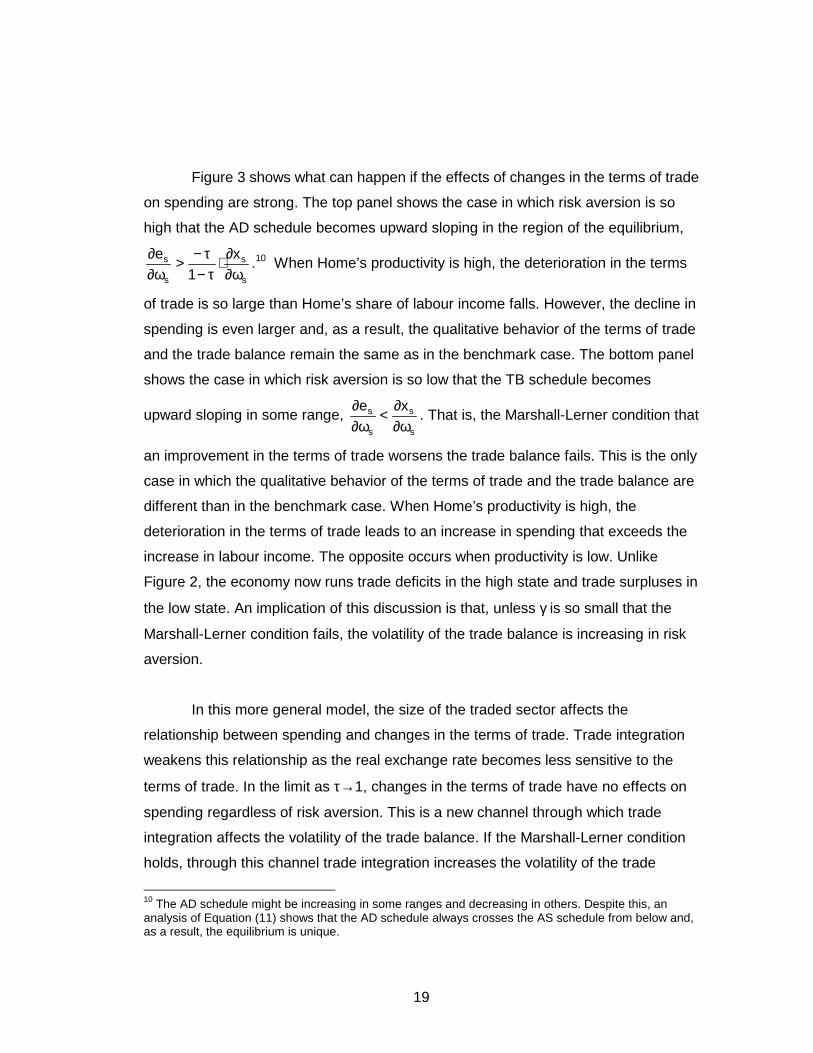
Figure 3 shows what can happen if the effects of changes in the terms of trade

on spending are strong. The top panel shows the case in which risk aversion is so

high that the AD schedule becomes upward sloping in the region of the equilibrium,

s

s

s

s x1

eω∂

∂⋅τ−τ−>

ω∂∂ .10 When Home’s productivity is high, the deterioration in the terms

of trade is so large than Home’s share of labour income falls. However, the decline in

spending is even larger and, as a result, the qualitative behavior of the terms of trade

and the trade balance remain the same as in the benchmark case. The bottom panel

shows the case in which risk aversion is so low that the TB schedule becomes

upward sloping in some range, s

s

s

s xeω∂

∂<ω∂

∂ . That is, the Marshall-Lerner condition that

an improvement in the terms of trade worsens the trade balance fails. This is the only

case in which the qualitative behavior of the terms of trade and the trade balance are

different than in the benchmark case. When Home’s productivity is high, the

deterioration in the terms of trade leads to an increase in spending that exceeds the

increase in labour income. The opposite occurs when productivity is low. Unlike

Figure 2, the economy now runs trade deficits in the high state and trade surpluses in

the low state. An implication of this discussion is that, unless γ is so small that the

Marshall-Lerner condition fails, the volatility of the trade balance is increasing in risk

aversion.

In this more general model, the size of the traded sector affects the

relationship between spending and changes in the terms of trade. Trade integration

weakens this relationship as the real exchange rate becomes less sensitive to the

terms of trade. In the limit as τ→1, changes in the terms of trade have no effects on

spending regardless of risk aversion. This is a new channel through which trade

integration affects the volatility of the trade balance. If the Marshall-Lerner condition

holds, through this channel trade integration increases the volatility of the trade

10 The AD schedule might be increasing in some ranges and decreasing in others. Despite this, an analysis of Equation (11) shows that the AD schedule always crosses the AS schedule from below and, as a result, the equilibrium is unique.

20

balance if risk aversion is low, but lowers it if risk aversion is high. If the Marshall-

Lerner condition fails, trade integration always lowers the volatility of the trade

balance through this channel.

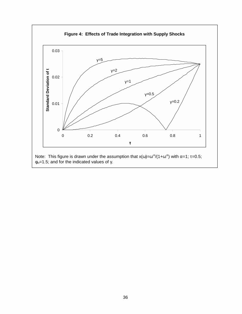
If risk aversion is high enough, or else sufficiently low that the Marshall-Lerner

condition fails, this new channel might be strong enough to generate a negative

relationship between trade integration and the volatility of the trade balance. Figure 4

illustrates this by plotting the volatility of the trade balance against the size of the

traded sector for different values of risk aversion. Not surprisingly, we find that at

values of γ that do not depart much from one, trade integration monotonically

increases the volatility of the trade balance. But if risk aversion is sufficiently extreme,

there might be some ranges in which an increase in the size of the traded sector

lowers the volatility of the trade balance.

The other polar case in which fluctuations are driven only by demand shocks

is much simpler to analyze. Naturally, if the effects of terms of trade changes on

Home’s share of spending are not too strong, i.e. s

s

s

s

s

s x1

exω∂

∂⋅τ−τ−≤

ω∂∂≤

ω∂∂ , the

qualitative description of the effects of supply shocks in Figure 2 still applies. But

even if risk aversion is so high that the AD schedule becomes upward sloping or so

low that the TB schedule becomes upward sloping, the qualitative description in

Figure 2 still applies. This is shown in Figure 5. The only difference with the

benchmark case is quantitative. If risk aversion is high, increases in spending are

reinforced by improvements in the terms of trade and this increases the volatility of

the trade balance with respect to the benchmark case of logarithmic preferences. If

risk aversion is low, the opposite applies. An implication is that the volatility of the

trade balance is increasing in risk aversion. Unlike the case of supply shocks, this

relationship holds at all levels of risk aversion.

As we have already discussed, in the more general case of this section trade

integration has the additional effect of weakening the effects of the terms of trade on

21

spending. In the economy with demand shocks, through this channel trade integration

increases the volatility of the trade balance if risk aversion is low, but lowers it if risk

aversion is high. It is conceivable that if risk aversion is high enough this effect

becomes strong enough to create a range in which trade integration reduces the

volatility of the trade balance. We have however been unable to find a numerical

example in which this happens. Figure 6, which is analogous to Figure 4, shows how

the volatility of the trade balance changes as the size of the traded sector increases

for different values of γ. In all cases, the relationship is monotonically increasing.

The results of this section can now be summarized as follows:

Result #3: If risk aversion is sufficiently higher or sufficiently lower than the

benchmark case of logarithmic preferences, trade integration might lead to a

reduction in the volatility of the trade balance.

Figure 4 provides examples that prove this claim.

To sum up, Result #1 provides theoretical support for the view that trade

integration raises the volatility of the trade balance. Results #2 and #3 qualify this

view by showing what can go wrong if the two conditions stated in Result #1 are

violated. These cases however do not seem likely to be empirically relevant.

3. An Application to Trade in Services

Our objective in this section is to develop a sense of the quantitative

importance of the effects of trade integration on the trade balance. To achieve this

goal, we calibrate the model and use it to study the effects of an increase in the

22

tradeability of services.11 While further trade integration is likely to occur in many

different industries, we think that the example of services is particularly interesting

given the glaring mismatch between the share of services in production and their

share in international trade. In industrial countries, the service sector accounts for

almost 70 percent of value added but only 20 percent of exports and imports. To a

large extent, this bias in trade flows is the result of both technological and policy-

induced barriers to trade in services. There are signs however that this is likely to

change in the near future.12

We interpret the two-country model in section 1 as describing the United

States (Home) and the rest of the O.E.C.D. countries (Foreign). We calibrate the

model using available data and then consider two scenarios. In the first one, we

increase the share of traded goods in services to half of that observed in the rest of

the economy. In the second one, we increase the share of traded goods in services to

that observed in the rest of the economy.

3.1 Calibration

To calibrate the model, we need three pieces of information: (1) the size of the

traded sector; (2) the relative technology schedule; and (3) the distribution of shocks.

11 Throughout this section, we will use the term services to refer to transportation, communication, utilities, wholesale and retail trade, FIRE (finance, insurance and real estate), and other services (notably health, education, and other professional services). 12 As the textbook example of haircuts suggests, many services are inherently more difficult to transport than manufactures and commodities. Services also tend to be more vulnerable to a wide variety of non-tariff barriers to trade, such as professional licensing requirements that discriminate against foreigners, domestic content requirements in public procurement, or poor protection of intellectual property rights. But this seems to be changing rapidly. The last decade has brought a series of technological improvements that are making many services increasingly tradeable. As a result of advances in telecommunications technology, outsourcing abroad of computer programming, data entry, and call center services is becoming common practice. With the appearance of e-commerce, wholesale/retail sales and brokerage services can now be offered worldwide online. And the development of new software has raised the ability of architectural, engineering and other types of consulting firms to better interact around the globe. But this is not all. Recent multilateral negotiations under the World Trade Organization’s General Agreement on Trade in Services have made substantial progress towards dismantling a wide array of policy-induced barriers to trade in services. The harmonization of rules and regulations within the European Union has also contributed to this process.

23

For reasons of data availability, we choose 1997 as the reference year, and we

discuss how to obtain each of these three items in turn.

Item 1. The size of the traded sector: In all industries, some goods are traded

while others are not. Our objective here is to determine the size of the traded sector

for the economy as a whole, and at the industry level. We do so by taking seriously

the theoretical implication that every traded good is produced either at home or

abroad. Define X and M as overall U.S. exports and imports, and let v be the share of

the U.S. in O.E.C.D. GDP in 1997. O.E.C.D. spending on U.S. exportables is X/(1-v).

This is the sum of foreign spending on U.S. exportables plus U.S. spending on these

exportables. The former is simply X, and since all countries distribute their spending

equally across goods, the latter is simply X⋅v/(1-v). Following the same argument, we

can calibrate O.E.C.D. spending on U.S. importables as M/v. This means that the

traded sector of the O.E.C.D. is X/(1-v)+M/v. To obtain the nontraded sector in the

U.S., we simply take gross output, G, and subtract the traded sector, X/(1-v). Under

the assumption that the U.S. share in O.E.C.D. production is the same as its share in

GDP, the non-traded sector of the O.E.C.D. is (G-X/(1-v))⋅(1-v)/v. We use data on G,

X, and M from the 1997 U.S. input-output table to compute the traded and nontraded

sectors and find that the share of traded goods, τ, is roughly 10 percent. 13

To obtain the size of the traded sector industry-by-industry, we repeat the

procedure using data on G, X and M for 33 3-digit industries spanning the entire

economy. The first column of Table 1 reports the share of tradeables in gross output

or production by industry. There are substantial differences in the share of traded

goods across industries. In services, which account for 62 percent of production,

tradeables represent only 3 percent of production. In the rest of the economy

(primarily manufacturing which accounts for 28 percent of production), tradeables

represent 22 percent of production.

13 Note that we are expressing tradeables as a fraction of production, rather than value added. For the U.S., the share of exports plus imports in value added in 1997 is 0.23.

24

Item 2. The relative technology schedule: We calibrate differences in industry

technologies to match data on trade in goods and services.14 To do so we need to

impose some additional structure on the data. In particular, we treat the distribution of

relative productivities within each of the 33 industries as unobservable, but assume

that it is well approximated by a lognormal distribution. This means that our calibration

procedure must come up with two parameters per industry, namely, the mean (µi) and

variance (σi) of log productivity differences. Unfortunately, we do not have enough

information to do so. We therefore set σi=σ=0.5 for all industries and use the trade

data to determine µi for each industry. This assumption means that we restrict the

relative productivity of goods in the 95th percentile to be roughly 5 times that of goods

in the 5th percentile within each industry. This does not seem unreasonable.

Moreover, we find that the results are robust to sensible changes in the value of σ.

Define the relative technology schedule for the traded sector of industry i

as)z(a)z(a)z(A

i

*i

i ≡ ; and order goods by using the rule that z≤z’ if and only if

)'z(a)'z(a

)z(a)z(a

i

*i

i

*i ≥ . Assume that, within an industry, the distributions of log productivities

in the traded and nontraded sectors are identical. Then, our assumptions imply that

),(N~)z(Aln ii σµ for industry i. To obtain the value of µi for each industry, note that on

average the share of exports in the traded sector of industry i corresponds to the

share of traded goods for which ω>)z(Ai . We therefore choose µi to ensure that

[ ] ii x)z(AP =ω> where v/M)v1/(X

)v1/(Xxii

ii +−

−= . Inverting this probability gives:

14 Could we have estimated productivity differences directly? A vast number of papers report cross-country estimates of productivity levels. However, only very few provide disaggregated productivity comparisons based on disaggregated purchasing power parity adjustments for inputs and outputs, which are essential for meaningful productivity level comparisons (see Harrigan (1999) for a review). Because of the difficulties in collecting disaggregated price data, these papers focus on only a subset of industries (for example, Harrigan (1999) reports estimates for machinery and equipment manufacturing productivity levels across several O.E.C.D. countries). But without information on productivity levels comparisons for all sectors and for all potential trading partners, it is impossible to construct a relative technology schedule.

25

(14) ( ) )x1(ln i1

i −Φ⋅σ−ω=µ −

where Φ(.) denotes the cumulative normal distribution function. To implement this

procedure, we need information on the average values of productivity-adjusted

relative wages, ω. We obtain average relative wages by equating the U.S. share of

O.E.C.D. income with the observed 40 percent U.S. share in O.E.C.D. GDP in 1997.

We interpret differences in average productivity as reflecting differences in human

capital between the U.S. and the rest of the O.E.C.D., and measure them using data

on years of total education.15 This leads us to an estimate of the productivity-adjusted

wage of 33.1=ω .

With this number at hand, and the assumption that σ=0.5, we use Equation

(14) to obtain a set of estimates for the µis. The results are shown in the third column

of Table 1. There are large differences across sectors in calibrated mean relative

productivities, ranging from 0.47 to 2.68. By construction, these differences in

average relative productivities reflect differences across industries in exports as a

share of tradeable production (reported in the second column of Table 1). Perhaps

the most noticeable feature of column 3 is again the difference between services and

the rest of the economy. Although tradeables as a fraction of services production is

quite small, exports as a share of tradeables is much larger in services than in the

rest of the economy (79 percent versus 30 percent). This implies that average relative

productivity must be substantially higher in services than in the rest of the economy

(2.54 versus 1.31).

Given values of µi obtained in this way, we can construct the empirical analog

of the inverse of the relative technology schedule as a weighted average of the

industry distributions of relative productivities:

15 Specifically we use the Barro-Lee (2000) data on human capital stocks to find that average total years of education in the U.S. and in the rest of the O.E.C.D. in 1995 are 12.2 and 8.3, respectively. We then assume a Mincer coefficient of 0.1, and adjust relative wages by a factor of 07.1e )3.83.12(1.0 =−⋅ .

26

(15) ( ) ( )∑=

−

σµ−ω

Φ−⋅=τ

τω≡τω33

1i

ii

1 ln1t;A);(x

where ti denotes the share of industry i in the overall traded sector. The results of this

procedure are depicted in Figure 7 under the label “baseline”. Note that there are

substantial cross-country differences in productivities. The ratio of productivities

between goods in the 95th and 5th percentiles is around 7.5.

The schedules labeled “Scenario 1” and “Scenario 2” correspond to our

assumptions that the share of traded goods in services increases from 2.5 to 10, and

to 22 percent, respectively. In particular, for each industry i within services, we

assume that the share of traded goods in that industry increases to half the level of

the trade share in the rest of the economy (in the first scenario), and increases all the

way to the level of the trade share in the rest of the economy (in the second

scenario). This in turn increases ti (the share of industry i in the overall traded sector)

for each of the industries within services, in Equation (15). To understand the effects

of trade integration on the relative technology schedule, remember that our

calibrations indicate that US relative productivity in services is substantially higher

than in the rest of the economy. This means that in our example, trade integration is

biased towards goods in which the U.S. has comparative advantage. As a result, the

relative technology schedule shifts to the right and becomes steeper than in the

benchmark case. Note also that such a rightward shift in the relative technology

schedule was not possible in the examples in Section 2 where we restricted attention

to the case of symmetric technology differences across countries.

Item 3. The distribution of shocks: We calibrate shocks to demand and supply

to match the cyclical properties of the U.S. trade balance. To do this, we first need to

know the value of the risk aversion coefficient, γ. It is clear from the discussion in

section 2 that this coefficient plays an important role in determining the volatility of the

trade balance. In the absence of strong priors on the magnitude of this parameter, we

27

consider scenarios in which γ takes the values 0.5, 1 and 5. We then assume that

there are two equally likely states of nature s=H,L; in which (φH,δH)=(φ,δ) and (φL,δL)=(

φ-1,δ-1). As in Section 2, the parameters φ and δ regulate the standard deviation of

shocks to supply and demand, respectively. We then choose φ and δ to match the

cyclical properties of the U.S. trade balance as a share of O.E.C.D. income over the

period 1970-1999, as summarized by (1) its standard deviation, which is 0.5 percent;

and (2) its comovement with income measured as the slope of a regression of the

U.S. trade balance on U.S. income (both as a share of O.E.C.D. income), which is –

0.3. We do this for each of the three values of the coefficient of relative risk aversion

that we consider.

The results of this procedure are presented in the first two columns of Table 2.

In the benchmark case of γ=1, a combination of supply shocks with a standard

deviation of 2 percent and demand shocks with a standard deviation of 10 percent

are required to match the cyclical properties of the trade balance. Since the U.S.

trade balance tends to decline when incomes are high, we require large demand

shocks and small supply shocks in order to match the data. If γ=5, we need a smaller

difference between demand and supply shocks (with standard deviations of 8 percent

and 5 percent, respectively). If γ=0.5, we need a larger differences in the volatility of

demand and supply shocks (with standard deviations of 17 percent and 3 percent

respectively) in order to match the observed cyclical properties of the trade balance.

To understand these differences, remember that fluctuations in the terms of trade

magnify (dampen) the effects of demand shocks if γ>1 (γ<1). This is why we need

smaller demand shocks the larger is γ.

3.2 Results

The remaining columns of Table 2 summarize the result of our trade

integration exercise, reporting the predicted standard deviation of the U.S. trade

28

balance as a fraction of O.E.C.D. income in the baseline 1997 scenario, and the two

integration scenarios discussed above. By construction, the standard deviation of the

trade balance is equal to its observed value of 0.5 percent of O.E.C.D. income in all

three rows of the first column. Moving to the right illustrates the effects of goods and

services trade liberalization on asset trade.

In the benchmark case of γ=1, we find quite substantial effects of further trade

integration on the volatility of the trade balance, which rises from 0.5 percent to 0.7

percent when services are half as tradeable as the rest of the economy, and to 0.9

percent when services are equally tradeable than the rest of the economy. This

suggests that the main effect of trade integration on the volatility of the trade balance

summarized in Result #1 is quantitatively important. On the other hand, Result #2

which qualifies our main result does not appear to be empirically very important.

Although in this example trade integration is biased towards goods in which the U.S.

has comparative advantage, we find that the quantitative effects of this bias are trivial.

To isolate the effects of this bias, we re-estimate Scenario 2, but do so under the

assumption that the relative technology schedule does not change relative to the

baseline scenario. In this case, we find that the standard deviation of the trade

balance is 0.95%, as opposed to 0.94% when we allow for a bias in trade integration.

Finally, the rows with γ=5 and γ=0.5 show the effects of trade integration when

we allow for the possibility that changes in the terms of trade also affect spending.16

When γ=5 we find that the effects of trade integration on the standard deviation of the

trade balance are substantially smaller, with the latter rising to only 0.6 percent in the

second integration scenario. To understand this difference, remember that when γ>1,

fluctuations in the terms of trade induce fluctuations in spending which amplify

fluctuations in the trade balance. As trade integration proceeds, the effects of

fluctuations in the terms of trade on spending fall, and so the volatility of the trade

16 Remember that we have re-calibrated the underlying shocks in each row of Table 2 to replicate observed fluctuations in the trade balance. As a result, changes in the volatility of the trade balance aross different values of γ for a given level of trade integration reflect changes in our assumptions about both (i) the shocks which drive fluctuations, and (ii) the degree of risk aversion.

29

balance increases by less than in the benchmark case of γ=1. When γ=0.5, we find a

much larger effect of trade integration on the volatility of the trade balance, with the

latter rising to 0.9 percent in the first scenario, and 1.2 percent in the second. The

intuition for this is just the converse of the case where γ=5: through their effects on

spending, fluctuations in the terms of trade attenuate fluctuations in the trade

balance, and the importance of this attenuation declines with trade integration.

To sum up, our empirical example suggests that the effects of trade

integration on the volatility of trade balance can be substantial, with the volatility of

the trade balance almost doubling in the benchmark case of log preferences.

Although in our example trade integration is biased towards goods in which the U.S.

has comparative advantage, the quantitative effects of this bias are negligible.

Departures from the assumption of log preferences do affect the quantitative effects

of trade integration, with larger (smaller) increases in the volatility of the trade balance

when risk aversion is low (high). However, in our calibrations the additional effects of

risk aversion are never sufficiently strong to reverse our qualitative conclusion that

trade integration will increase the volatility of the trade balance.

4. Concluding Remarks

In this paper, we have used a simple model of trade in goods and assets to

analyze the question of how trade integration affects the trade balance. We hope our

contribution will induce others to explore this issue from alternative theoretical

perspectives. We have motivated trade in goods and assets by postulating

differences in technology and imperfectly correlated shocks. But one could for

instance allow for differences in factor endowments and/or increasing returns to scale

as an additional motive for trade in goods. Similarly, one might introduce differences

in time preference and/or rates of return to capital as an additional motive to trade in

assets. We conjecture that the main results of this paper would survive in these more

30

general frameworks, except for extreme cases. The interesting question is whether

new and realistic effects would arise that cannot be studied in our simple framework.

Finally, we hope that our contribution also provides a good theoretical

grounding to empirical studies of the effects of trade integration. By isolating key

theoretical channels, the model here can sharpen the interpretation of econometric

studies on this subject. By providing a fully specified model, we also hope to aid in the

task of developing quantitative assessments of the effects of trade integration on the

trade balance. In this respect, our calibration exercise should be interpreted only as a

simple illustration or example. A serious quantitative analysis of the effects of trade

integration on the trade balance would be a major project on its own.

References

Baier, S.L. and J.H. Bergstrand [2001], “The Growth of World Trade: Tariffs, Transport Costs and Income Similarity,” Journal of International Economics, 53, 1, 1-27. Barro, R.J. and J. Lee [2000], "International Data on Educational Attainment: Updates and Implications," Harvard University Center for International Development Working Paper No. 42. Cole, H. and M. Obstfeld [1991], “Commodity Trade and International Risk Sharing: How Much Financial Markets Matter?” Journal of Monetary Economics, 28, 1, 3-24. Harrigan, J. [1999], “Estimation of Cross-Country Differences in Industry Production Functions,” Journal of International Economics, 47, 267-293. Dornbusch, R., S. Fischer and P. Samuelson [1977], “Comparative Advantage, Trade and Payments in a Ricardian Model with a Continuum of Goods,” American Economic Review, 67, 823-839.

31

Table 1: Trade and Relative Productivity by Industry

Average

Tradeables/ Exports/ RelativeProduction Tradeables Productivity(1)

Agriculture and MiningAgriculture 0.13 0.41 1.34Metallic ores mining 0.21 0.31 1.18Coal mining 0.09 0.84 2.46Crude petroleum and natural gas 0.38 0.03 0.60Nonmetallic minerals mining 0.11 0.29 1.15

ConstructionConstruction 0.00 0.00 0.47

ManufacturingFood 0.10 0.39 1.32Tobacco 0.15 0.74 2.08Textiles 0.17 0.32 1.19Apparel 0.44 0.09 0.78Lumber and wood products 0.15 0.22 1.03Furniture and fixtures 0.21 0.18 0.96Paper 0.16 0.36 1.25Printing 0.05 0.49 1.49Chemicals 0.26 0.39 1.30Petroleum Refining 0.11 0.33 1.22Rubber and Plastics 0.17 0.28 1.13Leather 0.75 0.06 0.71Nonmetal Production 0.16 0.23 1.04Primary Metals 0.22 0.22 1.02Fabricated metals 0.13 0.31 1.18Industrial Machinery 0.39 0.43 1.37Electrical machinery 0.50 0.31 1.18Motor Vehicles 0.37 0.16 0.92Other Transportation Equipment 0.44 0.51 1.53Other Manufacturing 0.40 0.30 1.16

ServicesTransportation Services 0.12 0.77 2.17Communications 0.00 0.00 0.89Electric Utilities 0.01 0.15 0.89Gas Utilities 0.00 0.00 0.89Trade 0.05 0.71 2.00FIRE 0.02 0.88 2.68Other Services 0.01 0.77 2.19

Weighted Averages (2)Overall 0.10 0.37 1.49Rest of Economy 0.22 0.30 1.31Services 0.03 0.79 2.54

Notes:

(1) This column reports 2/2

ie]iA[Eσ+µ

= (2) The first column uses shares in total production as weights; the remaining columns uses shares in

tradeables production as weights.

32

Table 2: Calibration Results

Standard Deviation of US Trade Balance/OECD GDP

Afterγ φ δ Before Scenario 1 Scenario 2

0.5 1.03 1.17 0.50% 0.91% 1.24%1 1.02 1.10 0.50% 0.74% 0.94%5 1.05 1.08 0.50% 0.58% 0.60%

Notes: (1) To obtain the standard deviation of the trade balance as a fraction of U.S. GDP simply multiply by 2.5.

33

Figure 1: Effects of Trade Integration on Relative Technology Schedule

Case 1: Trade Integration Weakens Comparative Advantage

0

1

2

0 0.5 1x

A( ττ ττ

x;ττ ττ)

, ωω ωω

Low τHigh τ

AB

B'

A'

Case 2: Trade Integration Strengthens Comparative Advantage

0

1

2

0 0.5 1x

A( ττ ττ

x;ττ ττ)

, ωω ωω

Low τ High τ

AB

B'A'

34

Figure 2: Effects of Supply and Demand Shocks, γγγγ=1

Supply Shocks

AS, ADTrade Balance 0

ASHASL

AD

TB

EH

ELEL

EH

ω

Demand Shocks

AS, ADTrade Balance 0

ASADHTBHTBL

EH

EL

ADL

EL

EH

ω

Note: These figures are drawn under the assumption that x(ω)=ω-α/(1+ω-α) with α=0.2; τ=0.5; φH=1.5 in the top panel and δH=1.5 in the bottom panel; and γ=1.

35

Figure 3: Effects of Supply Shocks

γ>>1

AS, ADTrade Balance 0

ASHASLADTB

EH

ELEL

EH

ω

γ<<1

AS, ADTrade Balance 0

ASHASL

AD

TB

EH

EL EL

EH

ω

Note: These figures are drawn under the assumption that x(ω)=ω-α/(1+ω-α) with α=0.2, τ=0.5; φH=1.5; and γ=5 in the top panel and γ=0.2 in the bottom panel.

36

Figure 4: Effects of Trade Integration with Supply Shocks

0

0.01

0.02

0.03

0 0.2 0.4 0.6 0.8 1

ττττ

Stan

dard

Dev

iatio

n of

t γ=2

γ=1

γ=5

γ=0.5

γ=0.2

Note: This figure is drawn under the assumption that x(ω)=ω-α/(1+ω-α) with α=1; τ=0.5; φH=1.5; and for the indicated values of γ.

37

Figure 5: Effects of Demand Shocks

γ>>1

AS, ADTrade Balance 0

ASADHTBHTBL

EH

EL

ADL

EL

EH

ω

γ<<1

AS, ADTrade Balance 0

ASADHTBHTBL

EH

EL

ADL

EL

EH

ω

Note: These figures are drawn under the assumption that x(ω)=ω-α/(1+ω-α) with α=0.2; τ=0.5; δH=1.5; and γ=5 in the top panel and γ=0.2 in the bottom panel.

38

Figure 6: Effects of Trade Integration with Demand Shocks

0

0.01

0.02

0.03

0.04

0.05

0 0.2 0.4 0.6 0.8 1

ττττ

Stan

dard

Dev

iatio

n of

t

γ=5γ=2

γ=1γ=0.5

γ=0.2

Note: This figure is drawn under the assumption that x(ω)=ω-α/(1+ω-α) with α=1; τ=0.5; δH=1.5; and for the indicated values of γ.

39

Figure 7: Estimated Relative Technology Schedule

0

0.5

1

1.5

2

2.5

3

3.5

4

4.5

5

0 0.1 0.2 0.3 0.4 0.5 0.6 0.7 0.8 0.9 1

x

A( ττ ττ

x;ττ ττ)

BaselineScenario 1Scenario 2