NBER WORKING PAPER SERIES THE NEW FAMA PUZZLE

NBER WORKING PAPER SERIES

THE NEW FAMA PUZZLE

Matthieu BussiereMenzie D. ChinnLaurent FerraraJonas Heipertz

Working Paper 24342http://www.nber.org/papers/w24342

NATIONAL BUREAU OF ECONOMIC RESEARCH1050 Massachusetts Avenue

Cambridge, MA 02138February 2018, Revised January 2022

We would like to thank Agnès Bénassy-Quéré, Yin-Wong Cheung, Alexander Chudik, Jeffrey Frankel, Jim Hamilton, Jean Imbs, Ben Johannsen, Joe Joyce, Steve Kamin, Evgenia Passari, Arnaud Mehl, Lucio Sarno, and conference participants at the Banque de France-Sciences Po. “Workshop on Recent Developments in Exchange Rate Economics,” the “Jean Monnet Workshop on Financial Globalization and its Spillovers,” and seminars at the Banque de France, ECB, Brandeis and the University of Adelaide, Dallas Fed, and UC Riverside. The views expressed do not necessarily reflect those of the Banque de France, the Eurosystem, or NBER.

At least one co-author has disclosed additional relationships of potential relevance for this research. Further information is available online at http://www.nber.org/papers/w24342.ack

NBER working papers are circulated for discussion and comment purposes. They have not been peer-reviewed or been subject to the review by the NBER Board of Directors that accompanies official NBER publications.

© 2018 by Matthieu Bussiere, Menzie D. Chinn, Laurent Ferrara, and Jonas Heipertz. All rights reserved. Short sections of text, not to exceed two paragraphs, may be quoted without explicit permission provided that full credit, including © notice, is given to the source.

The New Fama PuzzleMatthieu Bussiere, Menzie D. Chinn, Laurent Ferrara, and Jonas Heipertz NBER Working Paper No. 24342February 2018, Revised January 2022JEL No. F31,F41

ABSTRACT

We re-examine the historically common finding that ex post depreciation and the forward premium are negatively correlated, termed the forward premium puzzle. When covered interest differentials are zero, this finding is equivalent to the rejection of the joint hypothesis of uncovered interest parity (UIP) and full information rational expectations. We term this result the Fama puzzle (1984), given the difficulty in identifying a time-varying risk premium that could rationalize this result. In our analysis, the rejection occurs for eight exchange rates against the US dollar, but does not survive into the period during and in the decade after the financial crisis. Strikingly, in contrast to earlier findings, the Fama coefficient – the coefficient on the interest differential – then becomes large and positive; this is what we term the New Fama Puzzle. Using survey based measures of exchange rate expectations, we find much more constant evidence in favor of UIP. Hence, the explanation for the switch in the Fama coefficient in the wake of the global financial crisis is mostly a change in how expectations errors and interest differentials co-move.

Matthieu BussiereBanque de France31 rue Croix des Petits Champs75001 [email protected]

Menzie D. ChinnDepartment of EconomicsUniversity of Wisconsin-Madison1180 Observatory DriveMadison, WI 53706and [email protected]

Laurent FerraraSKEMA Business School5 Quai Marcel Dassault92150 [email protected]

Jonas HeipertzColumbia Business SchoolNew York, [email protected]

1

1. Introduction

The commonplace finding that ex post changes in exchange rates do not offset interest

differentials so as to equalize expected returns constitutes one of the durable puzzles in the

international finance literature. Empirically, this condition manifests itself in a negative

coefficient in a regression of exchange rate depreciation on interest differentials, which is often

termed the forward premium puzzle,1 documented in Fama (1984) and Tryon (1979), and what

we term the old Fama puzzle.

This finding seemingly contradicts one of the most central concepts in international

finance, namely uncovered interest rate parity. However, uncovered interest parity (UIP)

relates expected exchange rate changes to interest rate differentials. It’s only the joint

hypothesis of UIP and full information rational expectations – sometimes termed the

unbiasedness hypothesis – that leads to the implied value of unity for the regression coefficient

in the Fama (1984) regression. The most commonplace explanation for the rejection of the unit

coefficient – such as the existence of a time-varying exchange risk premium, which drives a

wedge between forward rates and expected future spot rates – has found little empirical

verification, despite numerous studies.2

We revisit this puzzle for several reasons, the most important of which is the finding

that the Fama coefficient has switched sign during the period starting with the global financial

1 If there are no covered interest differentials (as should be the case in the absence of capital controls and capital requirements), then the forward premium equals the interest differential. A regression of depreciation on the forward premium is equivalent to a regression of depreciation on interest differentials. We re-examine this point in the theoretical section. 2 In fact, Fama did not interpret the negative coefficient as a puzzle, as he attributed the result to the presence of a time varying risk premium. Engel (1996) surveys the failure of the portfolio balance models and consumption capital asset pricing models to provide a risk premium basis for the Fama result. See also Chinn (2006) and more recently Engel (2014).

2

crisis, and subsequently flipped sign again. It is this switching back and forth in a persistent

fashion that prompts our investigation of this “new” Fama puzzle.

Even without this back-and-forth result, one would have wanted to re-examine the

Fama result. First and foremost, interest rates in many advanced economies experienced a

prolonged period in which short rates effectively hit the effective lower bound, with a

corresponding compression of interest differentials, while ex post depreciations have not

exhibited a comparable reduction. Moreover, some measures of risk and uncertainty have risen

to record levels, raising the possibility that the effects of risk might be more easily detected

than in previous periods. The first point is clearly illustrated in Figure 1: where we plot one-

year interest rates for a set of eight selected countries and the United States. The commensurate

decline in interest differentials is shown in Figure 2. Figure 3 depicts the corresponding one

year exchange rate depreciations. These developments motivate us to re-examine whether the

Fama result is a general phenomenon or one that is regime-dependent.

The second point is illustrated by the plot of the VIX and the Economic Policy

Uncertainty Index, shown in Figure 4. This development potentially allows us to distinguish

between competing explanations for the failure of the unbiasedness hypothesis. Specifically,

we can examine whether the inclusion of these risk proxies alters the Fama result.3

To anticipate our results, we obtain the following findings. First, Fama’s (1984) finding

that interest rate differentials point in the wrong direction for subsequent ex-post changes in

exchange rates is by and large replicated in regressions for the full sample, ranging from

January 1999 to September 2021, but are really only replicated for the period 1999-2006. That

3 The question of exchange rate developments in light of interest rate differentials is obviously important for policy makers in general (and central bankers in particular, see for instance Coeuré, 2017).

3

is, the results change if the sample is broken into three periods – one before the global financial

crisis, one during and after, encompassing the effective lower bound era, and another one

largely corresponding to the period after the lift-off of US rates. For the middle period, interest

differentials correctly signal the right direction of subsequent exchange rate changes, but with

a magnitude that is not reconcilable with the conventional interpretation of UIP. In fact, we

obtain positive coefficients at exactly a time of high risk when it would seem less likely that

UIP would hold, presuming risk aversion explains deviations from UIP. Some months after

US rates rise above zero, the old Fama finding re-appears, and persists into the second episode

of zero lower bound rates.

We also find that the inclusion of a proxy variable for risk, namely the VIX, results in

Fama regression coefficients that are overall similar to those obtained without accounting for

risk aversion. This finding suggests that changes in the elevation of risk as measured by the

VIX do not explain the Fama puzzle, at least not in a direct linear fashion.

It is the use of expectations data that provides the following key insights. First, interest

differentials and anticipated exchange rate changes are overall positively correlated throughout

sample periods, consistent with the proposition that investors tend to equalize, at least partially,

returns expressed in common currency terms. The relationship between expected depreciation

and interest differentials also exhibits more stability than that involving ex post depreciation.

Second, in cases where the Fama coefficient switches sign from negative to positive, and

subsequently positive to negative, the result arises because the correlation of expectations

errors and interest differentials changes substantially. Hence, exchange risk does not appear to

be the primary reason why the Fama coefficient has been so large in recent years (although

that factor does play a role for certain currencies).

4

In the next section we briefly lay out the theory underlying the UIP and Fama

regressions, and review the existing literature. In Section 3, we examine the empirical results

obtained from estimating the Fama regression over different samples, and augmented with a

risk proxy. In Section 4 we explore the results dropping the full information rational

expectations assumption, and rely instead upon survey data on expectations. Section 5 presents

a decomposition of the components driving the deviation of the Fama coefficient from the

posited value of unity, and an economic interpretation for the changes we observe. Section 6

concludes.

2. Theory and Literature

One of the building blocks of international finance, the concept of uncovered interest parity

(UIP) is incorporated into almost all theoretical models. UIP is a no arbitrage profits condition:

(1) 𝐸𝐸𝑡𝑡𝑀𝑀[𝑠𝑠𝑡𝑡+ℎ − 𝑠𝑠𝑡𝑡] = (𝑖𝑖ℎ,𝑡𝑡 − 𝑖𝑖ℎ,𝑡𝑡∗ )

where 𝑠𝑠𝑡𝑡+ℎ − 𝑠𝑠𝑡𝑡 is the depreciation of the reference currency with respect to the foreign

currency from time 𝑡𝑡 to time 𝑡𝑡 + ℎ, 𝑖𝑖ℎ,𝑡𝑡 and 𝑖𝑖ℎ,𝑡𝑡∗ are the interest rates of horizon ℎ at time 𝑡𝑡 of

the reference and the foreign country, respectively. 𝐸𝐸𝑡𝑡𝑀𝑀 denotes the market’s expectation based

on time 𝑡𝑡 information. To fix ideas and to anticipate on the empirical results, let 𝑖𝑖ℎ,𝑡𝑡 represent

the US interest rate, 𝑖𝑖ℎ,𝑡𝑡∗ the foreign interest rate (that of the UK, euro area, Japan, etc), and s𝑡𝑡

the number of US dollars per foreign currency unit, such that an increase in s𝑡𝑡 is a depreciation

of the dollar. If the US interest rate, for any maturity h, is above, for example, Japan’s interest

rate, i.e. 𝑖𝑖𝑡𝑡 > 𝑖𝑖𝑡𝑡∗, then we should expect the dollar to depreciate with respect to the Japanese

yen at horizon h.

5

In other words, the market’s expectation of returns is equalized in common currency

terms, so that excess returns are not anticipated ex ante. In practice, the most common way in

which testing the validity of UIP has been implemented is by way of the Fama regression

(Fama, 1984), where the forward premium is treated as being equivalent to the interest

differential:4

(2) 𝑠𝑠𝑡𝑡+ℎ − 𝑠𝑠𝑡𝑡 = 𝛼𝛼 + 𝛽𝛽�𝑖𝑖ℎ,𝑡𝑡 − 𝑖𝑖ℎ,𝑡𝑡∗ � + 𝑢𝑢𝑡𝑡+ℎ

The OLS regression coefficient β is given by the following expression:

(3) �̂�𝛽 = 𝐶𝐶𝐶𝐶𝐶𝐶(𝑖𝑖ℎ,𝑡𝑡−𝑖𝑖ℎ,𝑡𝑡∗ ,𝑠𝑠𝑡𝑡+ℎ−𝑠𝑠𝑡𝑡)

𝑉𝑉𝑉𝑉𝑉𝑉(𝑖𝑖ℎ,𝑡𝑡−𝑖𝑖ℎ,𝑡𝑡∗ )

Under the joint null hypothesis of uncovered interest parity and rational expectations, 𝛽𝛽 = 1,

and the regression residual is a true random error term, orthogonal to the interest differential.

Note that the intercept 𝛼𝛼 may be non-zero while testing for UIP using equation (2). A non-zero

α may reflect a constant risk premium (hence, tests for β = 1 are tests for a time-varying risk

premium, rather than risk neutrality per se) and/or approximation errors stemming from

Jensen’s Inequality and from the fact that expectation of a ratio (the exchange rate) is not equal

to the ratio of the expectation.

In order to understand the surprising nature of the results for empirical tests of

uncovered interest parity, it is helpful to clarify what is to be expected from a Fama regression

4 For ease of exposition, log approximations are used. In the empirical implementation, exact formulas are used. We have examined data at three month and one year horizons (h ∈ [3,12]), using monthly data. This means the regression residuals are serially correlated under the null hypothesis of rational expectations and uncovered interest parity. We account for this issue by using robust standard errors. We report results for h=12, in order to conserve space; h=3 results are reported in the Appendix Tables 2-4.

6

by isolating the key assumptions necessary to go from equation (1) to regression equation (2).

There are three key assumptions, as laid out in the following equations:

(4) 𝑓𝑓ℎ,𝑡𝑡 − 𝑠𝑠𝑡𝑡 = �𝑖𝑖ℎ,𝑡𝑡 − 𝑖𝑖ℎ,𝑡𝑡∗ � − 𝜖𝜖ℎ,𝑡𝑡

𝑐𝑐𝑖𝑖𝑐𝑐,

(5) 𝑓𝑓ℎ,𝑡𝑡 = 𝐸𝐸𝑡𝑡𝑀𝑀[𝑠𝑠𝑡𝑡+ℎ] + 𝜖𝜖ℎ,𝑡𝑡𝑉𝑉𝑐𝑐 ,

(6) 𝑠𝑠𝑡𝑡+ℎ = 𝐸𝐸𝑡𝑡𝑀𝑀[𝑠𝑠𝑡𝑡+ℎ] − 𝜖𝜖𝑡𝑡+ℎ𝑓𝑓 .

When 𝜖𝜖ℎ,𝑡𝑡𝑐𝑐𝑖𝑖𝑐𝑐 is zero, then equation (4) indicates that there are no barriers to arbitrage using the

forward rate 𝑓𝑓ℎ,𝑡𝑡 (of horizon h, at time t). In other words, covered interest parity holds, or

equivalently, the covered interest differential is zero. This condition applies when capital

controls are not relevant, and there are no regulatory or funding constraints.5 For currency

pairs of advanced economies and for offshore yields (which we use),6 covered interest parity

has held up, up until the global financial crisis. Equation (5) indicates that the forward rate is

equal to the market’s expectation of the future spot rate up to an exchange risk premium term,

𝜖𝜖ℎ,𝑡𝑡𝑉𝑉𝑐𝑐 . This is tautology, unless greater structure is imposed.7

The combination of 𝜖𝜖ℎ,𝑡𝑡𝑐𝑐𝑖𝑖𝑐𝑐 = 𝜖𝜖ℎ,𝑡𝑡

𝑉𝑉𝑐𝑐 = 0 in Equations (4) and (5) yields uncovered interest

rate parity. Only when combined with the assumption of full information rational expectations,

namely 𝐸𝐸𝑡𝑡�𝜖𝜖𝑡𝑡+ℎ𝑓𝑓 � = 0 in equation (6)8, does one obtain the regression equation (2), where the

5 See Dooley and Isard (1980) for discussion and Popper (1993) for a review of the pre-2008 experience, in which the covered interest differential is attributed to political risk. 6 Note that we use offshore yields rather than sovereign bond yields, thereby mitigating the convenience yield channel emphasized by Engel (2016). 7 See Engel (1996) for a discussion of how the forward rate and the expected spot rate might deviate even under rational expectations and risk neutrality. 8 Note that the definition of the expectation or forecast error is the negative of the convention, i.e., actual minus forecast.

7

regression residual can be interpreted as the forecast error. In general, the 𝛽𝛽 = 1 hypothesis

relies upon three moment conditions:

(7) 𝑝𝑝𝑝𝑝𝑖𝑖𝑝𝑝(�̂�𝛽) = 1 −𝐶𝐶𝐶𝐶𝐶𝐶�𝑖𝑖ℎ,𝑡𝑡−𝑖𝑖ℎ,𝑡𝑡

∗ ,𝜖𝜖ℎ,𝑡𝑡𝑐𝑐𝑐𝑐𝑐𝑐�

𝑉𝑉𝑉𝑉𝑉𝑉�𝑖𝑖ℎ,𝑡𝑡−𝑖𝑖ℎ,𝑡𝑡∗ �

−𝐶𝐶𝐶𝐶𝐶𝐶�𝑖𝑖ℎ,𝑡𝑡−𝑖𝑖ℎ,𝑡𝑡

∗ ,𝜖𝜖ℎ,𝑡𝑡𝑟𝑟𝑐𝑐�



∗ ,𝜖𝜖𝑡𝑡+ℎ𝑓𝑓 �


When the covered interest differential is zero, the first covariance term is zero. This has been

the approach adopted historically; however, recent work has documented the fact that covered

interest differentials have increased in recent years even when using offshore rates (Borio et al.,

2016; Du et al., 2018), and so we do not impose this assumption in our analysis. In the absence

of covered interest differentials, as long as there is a time varying risk premium or biased

expectations, then 𝑝𝑝𝑝𝑝𝑖𝑖𝑝𝑝(�̂�𝛽) will deviate from unity.

The literature testing variants of the uncovered interest rate parity hypothesis is vast

and varied. Most of the studies fall into the category employing the full information rational

expectations hypothesis; in our lexicon, that means they are tests of the unbiasedness

hypothesis. Estimates of equation (6) using horizons for up to one year typically reject the

unbiasedness restriction on the slope parameter. For instance, the survey by Froot and Thaler

(1990), finds an average estimate for β of -0.88.9 Bansal and Dahlquist (2000) provide more

mixed results, when examining a broader set of advanced and emerging market currencies.

They also note that the failure of unbiasedness appears to depend upon whether the US interest

rate is above or below the foreign interest rate.10 11 Frankel and Poonawala (2010) document

9 Similar results are cited in surveys by MacDonald and Taylor (1992) and Isard (1995). Meese and Rogoff (1983) show that the forward rate is outpredicted by a random walk, which is consistent with the failure of the unbiasedness hypothesis. 10 Flood and Rose (1996, 2002) note that including currency crises and devaluations, one finds more evidence for the unbiasedness hypothesis. 11 See Hassan and Mano (2017) for a different perspective on how the Fama puzzle relates to the carry trade.

8

that for emerging markets more generally, the unbiasedness hypothesis coefficient is typically

more positive.12

The poor performance of the interest differential as a predictor shows up in other ways.

At short horizons, the interest differential is outperformed by a random walk model of the

exchange rate (Cheung et al., 2005; Cheung et al., 2019). However, at longer horizons, the

interest differential does much better than a random walk, mirroring the fewer rejections of the

unbiasedness hypothesis at longer horizons documented by Chinn and Meredith (2004).

There is an alternative approach that relaxes the rational expectations approach

involving the use of survey-based data to measure exchange rate expectations. In this case, the

error term in equation (6), 𝜖𝜖𝑡𝑡+ℎ𝑓𝑓 , need not be a true innovation. It could have a non-zero mean,

be serially correlated, and perhaps correlated with the interest differential. Froot and Frankel

(1989) were early expositors of this approach. In a related vein, Chinn and Frankel (1994)

document that it was more difficult to reject UIP for a broad set of currencies when using

survey based forecasts. Similar results were obtained by Chinn and Frankel (2020), when

extending the data up to 2018, increasing the sample to about 32 years. This pattern of findings

suggests that the assumption of full information rational expectations is not innocuous, and

that the examination of the UIP condition both dispensing with the rational expectation

assumption is warranted.

One approach we will not investigate is the bias arising from improper restrictions in

the estimation methodology, such as coefficient restrictions when there is substantial

12 Chinn and Meredith (2004) tested the UIP hypothesis at five year and ten year horizons for the Group of Seven (G7) countries, and found greater support for the UIP hypothesis holding at these long horizons than at shorter horizons of three to twelve months. The estimated coefficient on the interest rate differentials were positive and were closer to the value of unity than to zero in general.

9

persistence (Moore, 1994; Zivot, 2000), unbalanced regressions (Maynard and Phillips, 2001),

nonlinearity due to thresholds (Baillie and Kilic, 2006), and issues of cointegration (Chinn and

Meredith, 2005).

3. Fama Regressions

We collected monthly data for the interest rates and currencies of eight economies -- Canada,

Switzerland, Japan, Denmark, Norway, Sweden, UK and the euro area – over the Jan. 1999 –

September 2021 period. We examine twelve month exchange rate depreciation and the

corresponding offshore interest rates of twelve month maturities; the use of offshore interest

rates has historically obviated the need to account for the impact of capital controls.13

Figure 2: depicts twelve month maturity yield differentials, while Figure shows twelve

month depreciations, all over the 1999-2021 period. One of the contrasts clearly highlighted

by the two figures is that while yield differentials have shrunk toward zero in the wake of the

global financial crisis – at least until about 2015 --, exchange rate depreciations have not

exhibited a comparable compression.

Table 1 reports in Panel A the results from Equation (2) at the twelve month horizon,

for the full sample.14 The results are largely in accord with previous findings. The slope

coefficients on the interest differential (i.e., the “Fama regression slope coefficient”) are

negative, with the exception of Canada. Under the maintained hypothesis the coefficient should

13 We adopt the standard assumption of no default risk. In general, this is believed to hold, although during the height of the global financial crisis, counterparty risk was perceived as high (along with liquidity issues), so that covered interest parity did not hold (Coffey et al., 2009; Baba and Packer, 2009). 14 Since we are examining one year horizons, the interest rate sample is truncated at 2020M09.

10

be unity, which we test. In four cases, including the euro, one can reject the unit coefficient

null at the 1% level. The Canadian dollar, the Japanese yen, the Norwegian krone and British

pound fail to reject.15 Even when the coefficients are not significantly different from unity, it

is important to recall that the proportion of variation explained is very small.

The Fama regression represents a non-structural relationship. There is little reason to

believe the same results will hold over time. For instance, as policy regimes change, the

expectation formation process will change as well. Changes in the general economic

environment will also have an impact, possibly through regulations or global risk.

In order to identify break points in the Fama regression, we used the Bai (1997) and

Bai-Perron (1998) Sequential L+1 breaks vs. L test for structural breaks. While different break

points are identified for different exchange rates, the euro exchange rate (against the dollar) is

illustrative. Restricting the number of breaks to two, and using a 5% significance level, we

identify three periods: 1999M01-2005M04, 2005M05-2017M04, and 2017M05-2020M09.

For other exchange rates, we also identify two breakpoints, except for Switzerland and Norway

(for which we identify only one). However, even when two breakpoints are identified, the

second breakpoint is not usually the same.16 Nonetheless, we decide to use as a common

breakpoint those that apply to the euro.

15 Engel et al. (2021) finds weaker rejection of unbiasedness using a longer sample for the early period, and an alternative estimator for standard errors. They find in a 2007-2020 period, positive coefficients but a general failure to reject unity for the slope coefficient. 16 We have also conducted the analysis with a first breakpoint at 2006M08, and a second at 2018M01. That breakpoint incorporates exchange rate changes up to 2007M08, which could be considered as the beginning of the Global Financial Crisis, with the turmoil on the US housing market. Using this setup, we again obtain the same pattern of coefficient sign reversals.

11

There are several candidate events to associate with the first breakpoint. That time is

associated both with the ECB raising rates, and with US expected interest rates exceeding

actual rates. The second breakpoint is not clearly identified with any given event, although it

is about a year and a half after the increase in US policy rates, and underprediction of short

term interest rates.17 Consequently, we separate the sample into early, middle and late periods,

with ex post exchange rate depreciations ending April 2006, April 2018, and September 2021,

respectively. The respective subperiod results are presented in Panels B, C and D of Table 1.

In the pre-crisis (early) period, the coefficients are uniformly negative, and significantly

different from unity in all cases. Exchange rate depreciation is strongly -- and positively --

related to the interest differential. The estimated coefficients range from -2.1 to -5.2. The null

hypothesis of unity is rejected for all cases. The joint null hypothesis that the constant is zero

and the slope coefficient is unity is also uniformly rejected.

Turning the middle period, we obtain drastically different results. The slope coefficient

is positive in all instances. In five of eight cases, one can reject the null of a unit coefficient,

so even with the positive coefficient, the results are not consistent with the unbiasedness

hypothesis. To our knowledge, the only other study documenting something similar to our

findings is Baillie and Cho (2014). However, their analysis only extends up to 2012, while we

obtain this result over a period extending up to 2017.

In the late period, all the slope coefficients save Japan’s were negative – ranging from

-0.9 to -10.3. The null of a unit coefficient was rejected in all cases. One might think that

17 As indicated by the Survey of Professional Forecasters forecasts of the three month Treasury yield; this is discussed further in Section 5.

12

coefficients should switch back after the zero lower bound is re-attained. It is difficult to

determine whether this in fact occurs, given the few observations available especially when

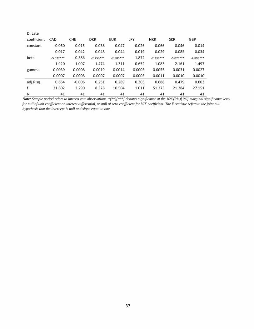
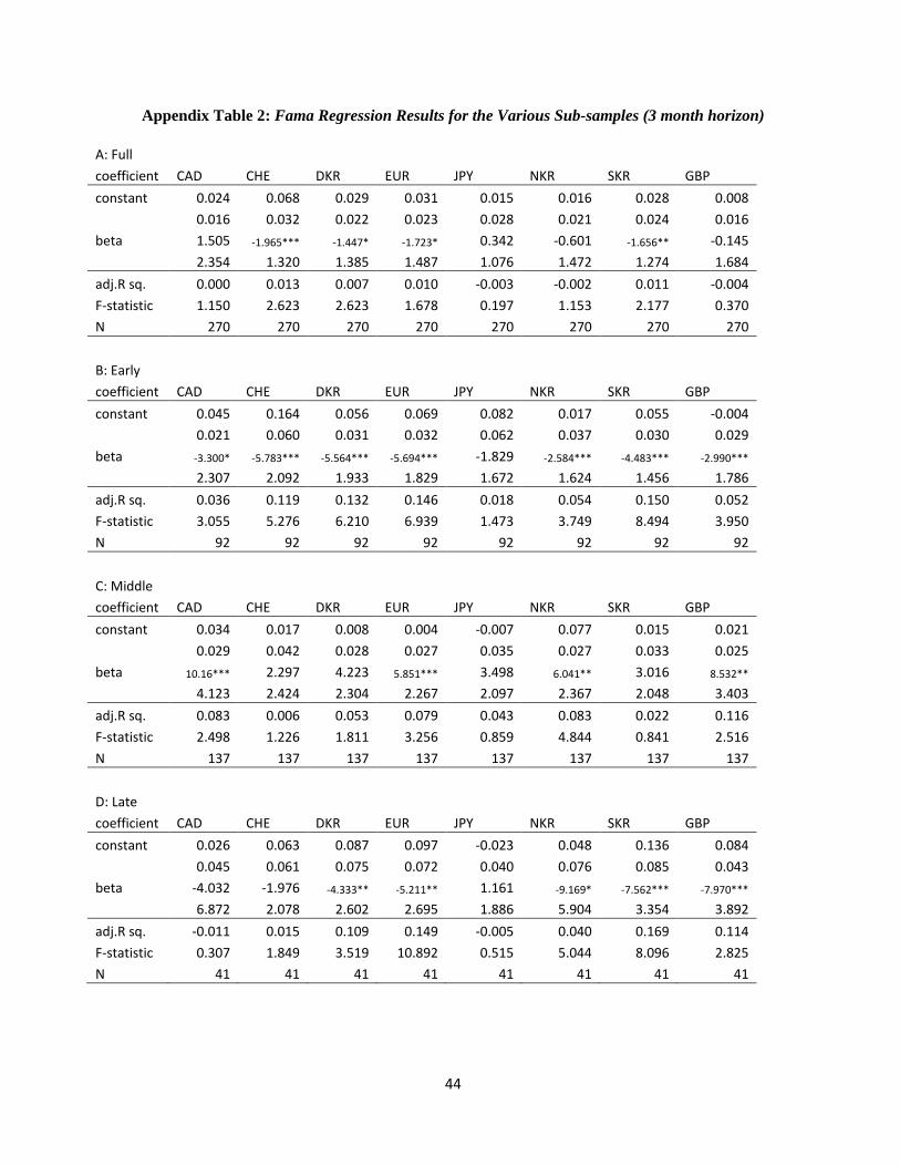
using the 12-month horizon. Using 3-month horizons, however, the slope coefficients remain

negative, albeit not always significantly so, after February 2020 (see tables in the Appendix).

To highlight the change in how the relationship between interest differentials and ex

post depreciations change over time, we focus on the Euro in Figure 5. The stabilization of the

interest differential, compared to pound depreciations, is now obvious. One way to illustrate

the contrast pre- and post-crisis, not necessarily evident in Figure 5, is to show a scatterplot of

depreciation against the yield differential. Figure 6 depicts the data for the three periods. In the

pre-crisis period, the slope is negative (as in the conventional empirical wisdom), while in the

post-crisis period, it is clearly positive. In the late period, the slope is again negative.18 Another

way to illustrate this finding is to show the evolution of the beta coefficients from rolling Fama

regressions. Figure 7 shows beta coefficients obtained from regressing the 12 month dollar

depreciation against the euro on the US-euro area interest differential, for three year rolling

windows. Results confirm the switch of signs of coefficients from negative to positive around

the beginning of 2006, and with less certainty a switch to negative again somewhere between

mid-2014 and mid-2016.

To highlight how the estimated beta coefficients evolve over time for all the currencies,

we show in Figure 8 the coefficients for the corresponding subperiods. In the top panel (early

period), the beta coefficients are tightly centered around negative values. In the middle panel

(middle period), the coefficients are positive and more widely spread. In the bottom panel (late

18 Appendix Figure 1 shows the corresponding graphs for all the currencies.

13

period), the estimates are mostly negative and very widely dispersed. The switch in slope

coefficient signs from the early to middle, and middle to late, holds across currencies with

strong regularity, with the sole exception of the Japanese yen. In that particular case, the

coefficient switches but once, from the early period to the middle period, and stays constant

thereafter.

Interestingly, the adjusted R2 rise substantially from essentially zero in the full sample

to values of around 0.2 to 0.8 in the various subsamples. From a statistical perspective, this

result is consistent with the conclusion that estimating over the full sample imposes restrictions

that are rejected by the data.19

One plausible criticism of our finding of sign switches is primarily driven by using the

dollar as a base currency. Remarkably, the switch from negative to positive coefficients holds

when examining exchange rates using other base currencies (see Appendix Table 1). The

switch from positive to negative coefficients in 2017 holds for fewer cross rates. Nonetheless,

this pattern of results indicates that there is at least one break in the Fama relationship for not

just those exchange rates expressed against the US dollar. These results confront the

researcher with at least two related questions. The first is the longstanding puzzle of why the

bias exists; the second is why the correlation changed so much after the crisis, and then again

seemingly reverted.

With respect to the first question, one approach is to allow for an exchange risk

premium, i.e., drop the assumption of 𝜖𝜖𝑡𝑡𝑉𝑉𝑐𝑐 = 0 (but retain the assumption of 𝜖𝜖𝑡𝑡

𝑐𝑐𝑖𝑖𝑐𝑐 = 0). Doing

19 The absolute size of the coefficients is larger after the first period; mechanically, this arises because the regression coefficient is a covariance divided by the variance of the interest differential, and the variance of interest differentials are much smaller post-Crisis, as illustrated in Figure 2.

14

so means that the error 𝑢𝑢𝑡𝑡+ℎ in 𝑠𝑠𝑡𝑡+ℎ − 𝑠𝑠𝑡𝑡 = 𝛼𝛼 + 𝛽𝛽�𝑖𝑖ℎ,𝑡𝑡 − 𝑖𝑖ℎ,𝑡𝑡∗ � + 𝑢𝑢𝑡𝑡+ℎ includes a term that is

potentially correlated with the interest differential. A potential solution is to include as an

additional regressor some variable that proxies for an exchange risk premium, 𝜖𝜖𝑡𝑡𝑉𝑉𝑐𝑐 . This

suggests the following regression equation:20

(8) 𝑠𝑠𝑡𝑡+ℎ − 𝑠𝑠𝑡𝑡 = 𝛼𝛼 + 𝛽𝛽�𝑖𝑖ℎ,𝑡𝑡 − 𝑖𝑖ℎ,𝑡𝑡∗ � + 𝛾𝛾𝑍𝑍𝑡𝑡 + 𝑢𝑢𝑡𝑡+ℎ,

where 𝑍𝑍 is a proxy variable.

We select the VIX as a proxy measure 21. The VIX is a commonly used measure of

(inverse) risk appetite, and has been shown to have substantial explanatory power for exchange

rates (Hossfeld and MacDonald, 2015, Ismailov and Rossi, 2018) and for excess returns

(Brunnermeier et al., 2008, Habib and Stracca, 2012, or Husted et al., 2018).22

The results of the VIX augmented Fama regressions are reported in Table 2 and are

notable in the following sense. The inclusion of the VIX does not alter the basic pattern of

results for the Fama coefficient estimates found in Panel A of Table 1. However, the estimate

of the VIX coefficient is typically positive in the full sample, though generally non-significant.

20 If the exchange risk premium is a mean zero random error term, there is no need to include a proxy variable. If, however, there is a central bank reaction function that essentially makes the error term correlated with the interest differential (as in a Taylor rule), then the estimates obtained from a simple Fama regression will be biased. Variants of this approach include McCallum (1994), in which the central bank responds to exchange rate depreciation, and Chinn and Meredith (2004), in which exchange rate depreciation feeds into output and inflation gaps that determine central bank policy rates. See also Mark and Wu (1998) and Engel (2014). 21 Note that we also evaluate inflation differentials (and industrial production growth differentials) as proxies for a premium, in this case a liquidity premium, in line with Engel et al.’s (2019) model of forward rate bias (and high interest-high value currencies). However, we do not obtain empirical evidence for the usefulness of those variables in explaining the Fama puzzle. 22 See Berg and Mark (2018) for discussion of uncertainty and the risk premium.

15

We also examined the impact of VIX inclusion in the three subsamples, but overall we

do not obtain any significant results. This result suggests that when the slope coefficients

switch sign, it’s not because of the omission of the VIX.23

4. Testing UIP with Survey Data

Another way of testing whether arbitragers equalize expected returns is by dropping the

assumption of mean zero expectations error, namely 𝐸𝐸𝑡𝑡�𝜖𝜖𝑡𝑡+1𝑓𝑓 � = 0 in equation (6). It might be

that agents are truly irrational, they use bounded rationality, or have not completely learned

the model governing the economy (or, as in Mark and Wu, 1998, some agents are noise

traders).

This means we replace equation (6) with:

(9) �̂�𝑠𝑡𝑡+ℎ𝑀𝑀 = 𝐸𝐸𝑡𝑡𝑀𝑀[𝑠𝑠𝑡𝑡+ℎ] − 𝜖𝜖𝑡𝑡+ℎ𝑀𝑀𝑓𝑓

The observed survey based measure of the future spot rate, �̂�𝑠𝑡𝑡+1𝑀𝑀 , equals the market’s

expectation, up to a mean zero random error.24 There is no assumption, then, that the ex ante

measure will be an unbiased measure of the ex post measure.

This substitution leads to the following regression equation (where we have not

suppressed the exchange risk premium):

(10) �̂�𝑠𝑡𝑡+ℎ𝑀𝑀 − 𝑠𝑠𝑡𝑡 = 𝛼𝛼 + 𝛽𝛽′�𝑖𝑖ℎ,𝑡𝑡 − 𝑖𝑖ℎ,𝑡𝑡∗ � + 𝑢𝑢𝑡𝑡

23 Kalemli-Ozcan and Varela (2021) investigate how the deviation from survey-implied UIP moves with the VIX, as opposed to how ex post depreciation moves. 24 In other words, we are assuming Classical measurement error, in line with most other analyses. Constant bias would be impounded in the constant. Time varying bias would be much more problematic.

16

In this case, the regression error impounds the forecast error; there is no guarantee that this

forecast error is mean zero, and uncorrelated with the interest differential -- or for that matter,

the risk proxy.

We use as measures of expectations survey data sourced from Consensus Forecasts

from 2003M01 to 2021M09. Notice that survey data availability necessitates a change in the

sample period.25

The results of the regressions are reported in Table 3, using the same format as in Table

1. One of the defining features of the results is (1) the point estimates are almost uniformly

positive (except for the Canadian dollar, in the early period), and (2) coefficients for the Swiss

franc in full and middle samples, and Japanese yen are in all samples, are significantly greater

than one, confirming that those currencies are considered as safe havens by practitioners.

Mechanically, the difference in estimated slope coefficients arises from the fact that ex ante

and ex post measures of depreciation differ substantially, so that the ex ante measures are

usually biased predictors. The rejection of the null hypothesis of unit coefficient, despite

positive estimates, can in part be attributed to the lower variability of ex ante depreciation,

leading to smaller estimated standard errors. These results are consistent with those obtained

in previous studies using survey data, including Chinn and Frankel (1993) and Chinn and

Frankel (2020)26.

25 An additional complication is that the interest rates and exchange rates do not align precisely in this data set. Interest rates are sampled at end-of-month, while exchange rates forecasts are sampled usually at the second Monday of the month by Consensus Forecasts. We have cross checked the results for the euro using Currency Forecasters Digest/FX Forecasts data (as used in Chinn and Frankel, 2020). The results are the same when the expected, futures and spot rates are exactly aligned. 26 Skeptics of survey based measures argue that reported forecasts are read off of interest differentials. Chinn and Frankel (1993) note the pattern of relationship between expected spot rates and forwards was consistent with the idea that survey respondents use other information in judging future exchange rate movements. In addition,

17

Why are the results so different going from the ex post to ex ante measures? The reason

is that the two measures of exchange rate depreciation differ widely and that the variation in

ex ante measures is substantially smaller than that of ex post measures. For instance, for the

euro dollar exchange rate, the one year ex ante changes range from -0.10 to +0.07; ex post

changes range from -0.22 to +0.26. The corresponding standard deviations are 0.037 and 0.100,

respectively. Roughly speaking, ex post changes are about three times as large as ex ante, for

the euro.

Table 3 displays the estimated β’ coefficients in the full sample as well as in the three

sub-periods. Turning to the full sample results in Panel A, in contrast to the results using ex

post depreciation, the coefficient on the interest differential is almost always positive. That

does not mean that uncovered interest parity holds, as less than half of the cases reject the null

of a unit slope coefficient (interestingly, not the euro). And in fact, for all cases save the

Canadian dollar the joint null hypothesis of a zero constant and unit slope is resoundingly

rejected. Interestingly, the sub-period point estimates (Panels B-D) do not suggest a switch in

coefficient signs through the three periods.

Our findings of positive coefficients might be interpreted as an artifact of subsample

selection. Applying Bai-Perron tests to the data indicate one or multiple breaks in all cases,

even when using a high significance level. However, the estimated slope coefficients for the

separate subperiods are all positive.

In sum, our empirical results indicate largely negative correlations between ex post

depreciation in the early and late periods, and largely positive correlations during the middle

Cheung and Chinn (2001) survey foreign exchange traders, and find that interest differentials are only one of the inputs forecasters use.

18

period. Inclusion of a conventional risk proxy, the VIX, does not alter these basic results. On

the other hand, expected depreciation and the interest differential is almost always positively

correlated.

5. Reconciling the Results

The contrasting results obtained using ex ante and ex post depreciation suggests that

understanding the characteristics of exchange rate expectations are critical to solving the

puzzle.

To see this point explicitly, consider again the decomposition outlined in equation (7), that is:

𝑝𝑝𝑝𝑝𝑖𝑖𝑝𝑝��̂�𝛽� = 1 −𝐶𝐶𝐶𝐶𝐶𝐶�𝑖𝑖ℎ,𝑡𝑡−𝑖𝑖ℎ,𝑡𝑡

∗ ,𝜖𝜖ℎ,𝑡𝑡𝑐𝑐𝑐𝑐𝑐𝑐�

𝑉𝑉𝑉𝑉𝑉𝑉�𝑖𝑖ℎ,𝑡𝑡−𝑖𝑖ℎ,𝑡𝑡∗ ��

𝐴𝐴


∗ ,𝜖𝜖ℎ,𝑡𝑡𝑟𝑟𝑐𝑐�

𝑉𝑉𝑉𝑉𝑉𝑉�𝑖𝑖ℎ,𝑡𝑡−𝑖𝑖ℎ,𝑡𝑡∗ ��

𝐵𝐵


∗ ,𝜖𝜖𝑡𝑡+ℎ𝑓𝑓 �


��

𝐶𝐶

,

where the relevant interest differential regression coefficients with the covered interest

differential, exchange risk, and expectation errors are labelled A, B, and C, respectively. From

this decomposition, it is clear that an increase in the estimated β coefficients could in principle

be due to a decrease in A, B, or C. The fact that the use of survey expectations reduces the

presence of coefficient switches suggests that the C term, involving forecast errors, is of crucial

importance.

In order to examine this conjecture more formally, we examine the regression

coefficients conforming to A, B, and C inverted so as to present a decomposition of estimated

(black squares) from UIP coefficient minus one value (i.e., 0), for the early, middle, and late

periods, respectively. Because our survey data only begins in 2003, we start our estimates for

19

all coefficients at that date (hence these estimated β coefficients for early period differ from

those reported in Panel B of Table 1).

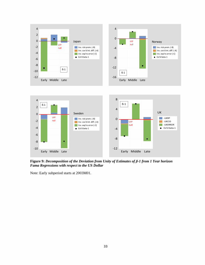
Estimates at the twelve month horizon are presented in Figure 9. For all the currencies

save the Canadian dollar, the coefficient estimate swings from negative to positive moving

from the early to middle period (the Canadian dollar’s coefficient is just above zero, switching

to large positive). In all cases, the correlation between expectations errors and interest

differentials swings from positive to negative, or becomes substantially less positive

(Switzerland and Japan). To be concrete, in the pre-crisis period, forecast errors defined as

𝐸𝐸𝑡𝑡𝑀𝑀[𝑠𝑠𝑡𝑡+ℎ] − 𝑠𝑠𝑡𝑡+ℎ are positively correlated with �𝑖𝑖ℎ,𝑡𝑡 − 𝑖𝑖ℎ,𝑡𝑡∗ � (showing up as a negative

component in the decomposition); that correlation is very negative in the middle period

(showing up as above zero in the figures). Since these components are subtracted from the

value of unity, that drives estimated Fama coefficients from negative to positive values.

Notice that the switch in the risk premium component – the B term – is not particularly

central to the switch in the Fama regression slope coefficient for any of the currencies. The

foregoing discussion suggests that the reason the puzzle has evolved in going from early to

middle period is mainly because of a change in how expectations errors co-move with interest

differentials, i.e., the C component.

The sign of the coefficient on the interest differential changes again – from positive to

negative -- moving from the middle to late period for all the currencies, save the Japanese yen.

There the correlation switches, but in a way that is opposite that for the other currencies. The

Swiss franc slope coefficient sign switches too, but in this case it’s a change in the exchange

risk premium correlation which drives the switch. The C component is unchanged in this case.

20

In the other six cases, the switch in how expectations errors move with the interest differential

drives the switch in the Fama regression coefficient sign.

What lies behind the change in the C component? For these currencies – save the

Japanese yen – the forecast errors as defined in equation (6) change from significantly negative

in the pre-crisis period to half positive in the middle crisis period. Finally, in the late period,

the dollar appreciates more than expected, except with respect to the Swiss France. In fact, the

Swiss franc is the only case for which the dollar constantly depreciates against more than

expected. The forecast errors – over- or underprediction – do not correspond to the switches

in slope coefficient in the Fama regression.

In words, the overprediction of dollar depreciation is systematically greater, the greater

the US-foreign interest differential. One of the characteristics of the 2005-17 period is that for

most of the period, US interest rates were consistently expected to rise faster than they actually

did. This point is illustrated in Figure 10, which shows the US three month Treasury yield and

the corresponding forecasts for up to one year as of the third quarter of each year. To the extent

that higher rates are associated with a stronger currency, the fact that rates did not rise in line

with expectations meant that the dollar ended up being weaker than anticipated – hence the

greater than anticipated dollar depreciation.

This means the reversals in the Fama coefficients is due in part to the larger mistakes

in forecasting dollar changes in the post-crisis period, and very little is attributable to changes

21

in exchange risk co-movements. And still less is associated with covered interest differentials

co-movements.27

6. Conclusions

Our extensive cross-currency analysis of uncovered interest parity has yielded new

empirical results that establish a new set of stylized facts.

First, the bivariate relationship between ex post depreciation and interest differentials,

as summarized in the Fama regression, is subject to breaks. While such breaks have shown up

in previous studies, the breaks associated with the global financial crisis and the subsequent

period of low interest rates, and the subsequent reversal, are quantitatively and qualitatively

much more pronounced. The positive, albeit very large, Fama regression coefficient detected

in much of the last decade is not usually consistent with uncovered interest parity. Moreover,

even if the coefficient magnitude were consistent with UIP, the finding would run counter to

the intuition that UIP should hold when risk is not important.

Second, we find that the inclusion of a proxy variable for risk, in the form of the VIX,

results in Fama regression coefficients that are largely unchanged. Hence, the Fama puzzle is

not explained by risk, at least when proxied by the VIX in a linear specification.

Third, uncovered interest parity regressions estimated using survey data are less

indicative of breaks. That finding suggests that the breakdown in the Fama relationship is

related to the nature of expectations errors.

27 At the three-month horizon, the A component is slightly more important, but remains less significant than the B and C components.

22

Fourth, a formal decomposition of deviations from the posited value of unity in the

Fama regression indicates that the switch in signs from the early to middle period can largely

be attributed to the switch in the nature of the co-movement between expectations errors and

interest differentials. We find that the switch does not tightly correspond to the period of

extended zero lower bound in the US. Rather the break coincides with persistent overprediction

of the US short term interest rate and hence overprediction of dollar strength.

From these results, we conclude that the change in the Fama coefficients is one that is

primarily driven by systematic expectational errors ruled out in the full information rational

expectations framework. Risk – either time varying or time invariant – might be important, but

it is not primarily important in driving ex post exchange rate changes.

REFERENCES

Baba, Naohiko, and Frank Packer, 2009, "From turmoil to crisis: dislocations in the FX swap market before and after the failure of Lehman Brothers." Journal of International Money and Finance 28(8): 1350-1374.

Baillie, Richard T. and Dooyeon Cho, 2014, "Time variation in the standard forward premium regression: Some new models and tests." Journal of Empirical Finance 29: 52-63.

Baillie, Richard T., and Rehim Kilic, 2006, "Do asymmetric and nonlinear adjustments explain the forward premium anomaly?" Journal of International Money and Finance 25(1): 22-47.

Bansal, Ravi, and Magnus Dahlquist, 2000, "The forward premium puzzle: different tales from developed and emerging economies." Journal of international Economics 51(1): 115-144.

Berg, Kimberly and Nelson Mark, 2018, “Measures of Global Uncertainty and Carry Trade Excess Returns,” Journal of International Money and Finance 88: 212-227.

Borio, Claudio, Robert Neil McCauley, Patrick McGuire and Vladyslav Sushko, 2016, “Covered interest parity lost: understanding the cross-currency basis,” BIS Quarterly Review, September 2016: 45-64.

23

Brunnermeier, Markus, Stefan Nagel, and Lasse H. Pedersen, 2008, “Carry Trades and Currency Crashes,” NBER Macroeconomics Annual, 2008 (Feb.)

Cheung, Yin-Wong and Menzie Chinn, 2001, “Currency traders and exchange rate dynamics: a survey of the US market,” Journal of International Money and Finance 20: 439-471.

Cheung, Yin-Wong, Menzie Chinn and Antonio Garcia Pascual, 2005, “Empirical Exchange Rate Models of the Nineties: Are Any Fit to Survive?” Journal of International Money and Finance 24 (November): 1150-1175.

Cheung, Yin-Wong, Menzie Chinn, Antonio Garcia Pascual, and Yi Zhang, 2019, “Exchange Rate Prediction Redux: New Models, New Data, New Currencies,” Journal of International Money and Finance 95: 332-362.

Chinn, Menzie, 2006, “The (Partial) Rehabilitation of Interest Rate Parity: Longer Horizons, Alternative Expectations and Emerging Markets,” Journal of International Money and Finance 25(1) (February): 7-21.

Chinn, Menzie and Jeffrey Frankel, 2020, “A Third of a Century of Currency Expectations Data: The Carry Trade and the Risk Premium,” mimeo (June).

Chinn, Menzie and Jeffrey Frankel, 1994, "Patterns in Exchange Rate Forecasts for 25 Currencies." Journal of Money, Credit and Banking 26(4): 759-770.

Chinn, Menzie and Guy Meredith, 2004, “Monetary Policy and Long Horizon Uncovered Interest Parity.” IMF Staff Papers 51(3): 409-430.

Chinn, Menzie and Guy, Meredith, 2005, “Testing Uncovered Interest Parity at Short and Long Horizons during the Post-Bretton Woods Era,” NBER Working Paper No. 11077 (January).

Coffey, Niall, Warren B. Hrung, and Asani Sarkar, 2009, “Capital Constraints, Counterparty Risk, and Deviations from Covered Interest Rate Parity,” Federal Reserve Bank of New York Staff Reports no. 393 (October).

Cœuré, Benoît, 2017, “The international dimension of the ECB’s asset purchase programme,” Speech at the Foreign Exchange Contact Group meeting, 11 July 2017.

Dooley, Michael P., and Peter Isard, 1980, "Capital Controls, Political Risk, and Deviations from Interest-rate Parity." Journal of Political Economy 88(2): 370-384.

Du, Wenxin, Alexander Tepper, Adrien Verdelhan, 2018, “Deviations from Covered Interest Rate Parity,” The Journal of Finance 73(3): 915-957.

Engel, Charles, 1996, “The Forward Discount Anomaly and the Risk Premium: A Survey of Recent Evidence,” Journal of Empirical Finance. 3 (June): 123-92.

Engel, Charles, 2014, “Exchange Rates and Interest Parity.” Handbook of International Economics, vol. 4, pp. 453-522.

24

Engel, Charles, 2016, “Exchange Rates, Interest Rates, and the Risk Premium,” American Economic Review 106: 436-474.

Engel, Charles, Dohyeun. Lee, Chang Liu, Chenxin Liu and Steve Pak Yeung Wu, 2019, “The uncovered interest parity puzzle, exchange rate forecasting and Taylor rules.” Journal of International Money and Finance 95: 317-331.

Engel, Charles, Ekaterina Kazakova, Mengqi Wang, Nan Xiang, 2021, “A Reconsideration of the Failure of Uncovered Interest Parity for the U.S. Dollar,” forthcoming, International Seminar on Macroeconomics, NBER.

Fama, Eugene, 1984, "Forward and Spot Exchange Rates." Journal of Monetary Economics 14: 319-38.

Fernald, J., T. Mertens and P. Shultz, 2017, “Has the dollar become more sensitive to interest rates?”, FRBSF Economic Letter, 2017-18, June 2017.

Flood, Robert P. and Andrew K. Rose, 1996, “Fixes: Of the Forward Discount Puzzle,” Review of Economics and Statistics: 748-752.

Flood, Robert P., and Andrew K. Rose, 2002, "Uncovered interest parity in crisis." IMF Staff Papers 49(2): 252-266.

Frankel, Jeffrey and Menzie Chinn, 1993, "Exchange Rate Expectations and the Risk Premium: Tests for a Cross Section of 17 Currencies." Review of International Economics 1(2): 136-144.

Frankel, Jeffrey, and Jumana Poonawala, 2010, "The forward market in emerging currencies: Less biased than in major currencies." Journal of International Money and Finance 29.3: 585-598.

Froot, Kenneth and Jeffrey Frankel, 1989, "Forward Discount Bias: Is It an Exchange Risk Premium?" Quarterly Journal of Economics. 104(1) (February): 139-161.

Froot, Kenneth A., and Richard H. Thaler, 1990, "Anomalies: foreign exchange," The Journal of Economic Perspectives 4(3): 179-192.

Habib, Maurizio M., and Livio Stracca, 2012, "Getting beyond carry trade: What makes a safe haven currency?." Journal of International Economics 87(1): 50-64.

Hassan, Tarek, and Rui Mano, 2017, “Forward and spot exchange rates in a multi-country world.” Mimeo (January).

Hossfeld, Oliver, and Ronald MacDonald, 2015, "Carry funding and safe haven currencies: A threshold regression approach." Journal of International Money and Finance 59: 185-202.

Husted, Lucas, John H. Rogers, and Bo Sun, forthcoming, “Uncertainty, Currency Excess Returns, and Risk Reversals,” Journal of International Money and Finance 88: 228-241.

Ismailov, Adilzhan and Barbara Rossi, 2018, “Uncertainty and Deviations from Uncovered Interest Rate Parity,” Journal of International Money and Finance 88: 242-259.

25

Kalemli-Özcan, Ṣebnem, and Liliana Varela, 2021, “Five Facts about the UIP Premium,” NBER Working Paper No. w28923.

MacDonald, Ronald and Mark P. Taylor, 1992, “Exchange Rate Economics: A Survey,” IMF Staff Papers 39(1): 1-57.

McCallum, Bennett T., 1994, "A reconsideration of the uncovered interest parity relationship." Journal of Monetary Economics 33(1): 105-132.

Mark, Nelson C., and Yangru Wu, 1998, "Rethinking deviations from uncovered interest parity: the role of covariance risk and noise." The Economic Journal 108(451): 1686-1706.

Maynard, Alex, and Peter CB Phillips, 2001, "Rethinking an old empirical puzzle: econometric evidence on the forward discount anomaly." Journal of applied econometrics 16(6): 671-708.

Moore, Michael J., 1994, “Testing for Unbiasedness in Forward Markets,” The Manchester School 62 (Supplement):67-78

Tryon, Ralph W., 1979, “Testing for rational expectations in foreign exchange markets,” International Finance Discussion Paper No. 139.

Zivot, Eric, 2000, “Cointegration and Forward and Spot Exchange Rate Regressions,” Journal of International Money and Finance 19(6): 785-812.

26

-1

0

1

2

3

4

5

6

7

8

00 02 04 06 08 10 12 14 16 18 20

I_12_CA I_12_CH I_12_DKI_12_EA I_12_JP I_12_NOI_12_SW I_12_UK I_12_US

Figure 1: Interest Rates on 1Year Eurocurrency Deposits, %

27

-6

-4

-2

0

2

4

6

8

00 02 04 06 08 10 12 14 16 18 20

I_12_US-I_12_CA I_12_US-I_12_CHI_12_US-I_12_DK I_12_US-I_12_EAI_12_US-I_12_JP I_12_US-I_12_NOI_12_US-I_12_SW I_12_US-I_12_UK

Figure 2: 1Year Eurocurrency Deposit Rates Differential (US Dollar minus Foreign Currency), %

28

-.4

-.3

-.2

-.1

.0

.1

.2

.3

.4

00 02 04 06 08 10 12 14 16 18 20

CADEP12 CHDEP12 DKDEP12 EADEP12JPDEP12 NODEP12 SWDEP12 UKDEP12

Figure 3: 1 Year Ex-Post Depreciation Rate of the US Dollar with respect to Foreign Currency (Positive values indicate dollar depreciations), decimal format

29

Figure 4: VIX (left scale) and US Economic Policy Uncertainty index (right scale), both end-of-period.

-.02

-.01

.00

.01

.02

.03

.04

-.3

-.2

-.1

.0

.1

.2

.3

00 02 04 06 08 10 12 14 16 18 20

EA12DIF (left scale)EADEP12 (right scale)

Figure 5: 1 Year Eurocurrency Deposit Rates Differential and 1Y-Ex-Post Depreciation Rate of the US Dollar with respect to euro (decimal format)

30

Panel (a): Early (pre-crisis)

Panel (b): Middle (Crisis/Post-Crisis)

Panel (c): Late

Figure 6: Scatterplot of the 1 Year Ex-Post Depreciation Rate (1 Year Ahead) on 1 Year Eurodeposit Rate Differential of US Dollar with respect to the Euro (decimal format)

Note: Regression line in red.

-.3

-.2

-.1

.0

.1

.2

.3

-.03 -.02 -.01 .00 .01 .02 .03

1 year US-euro area interest differential

1 ye

ar e

x po

st d

epre

ciat

ion

2005M05-2017M04

31

-25

-20

-15

-10

-5

0

5

10

15

2002 2004 2006 2008 2010 2012 2014 2016 2018

Figure 7: Estimates of Beta from a 1 Year horizon Fama Regression Euro with respect to the US Dollar 3 Year Rolling Windows (timing refers to interest differentials)

Figure 8: Estimates of Beta from a 1 Year horizon Fama Regression for Early, Middle, and Late Periods

-12

-8

-4

0

4

8

12

Early Middle Late

Inv. risk prem. (-B)Inv. cov'd int. diff. (-A)Inv. exp'ns error (-C)Est'd beta-1

ß-1

UIPnull

Canada

-12

-10

-8

-6

-4

-2

0

2

4

Early Middle Late


ß-1 UIPnull

Switzerland

32

-10

-8

-6

-4

-2

0

2

4

Early Middle Late


ß-1

UIPnull

Denmark

-10

-8

-6

-4

-2

0

2

4

6

Early Middle Late


ß-1

UIPnull

Euro

33

Figure 9: Decomposition of the Deviation from Unity of Estimates of β-1 from 1 Year horizon Fama Regressions with respect to the US Dollar

Note: Early subperiod starts at 2003M01.

-12

-10

-8

-6

-4

-2

0

2

4

Early Middle Late


ß-1

UIPnull

Japan

-16

-12

-8

-4

0

4

Early Middle Late


ß-1

UIPnull

Norway

-10

-8

-6

-4

-2

0

2

4

Early Middle Late


ß-1

UIPnull

Sweden

-12

-8

-4

0

4

8

Early Middle Late

-UKRP-UKCID-UKERROREst'd beta-1

ß-1

UIPnull

UK

34

0

1

2

3

4

5

6

7

00 02 04 06 08 10 12 14 16 18 20

GS3M GS3M_1YRFCAST1

Figure 10: Three month Treasury yield and Survey of Professional Forecasters mean forecast as of Q3, in %. Green shading denotes early, late periods.

Table 1: Fama Regression Results

A: Full coefficient CAD CHE DKR EUR JPY NKR SKR GBP constant 0.012 0.051 0.017 0.017 0.008 -0.002 0.011 -0.004

0.010 0.021 0.015 0.016 0.022 0.014 0.017 0.010 beta 1.310 -1.420*** -1.045*** -1.019*** -0.058 -0.583 -1.084*** -0.108 1.588 0.872 0.909 0.988 0.755 0.944 0.942 1.109 adj.R sq. 0.010 0.036 0.018 0.015 -0.004 0.003 0.018 -0.004 F-statistic 3.606 10.684 5.699 4.947 0.033 1.737 5.815 0.054 N 261 261 261 261 261 261 261 261

B: Early coefficient CAD CHE DKR EUR JPY NKR SKR GBP constant 0.037 0.137 0.056 0.068 0.086 0.017 0.048 0.006

0.010 0.022 0.014 0.014 0.023 0.018 0.017 0.021 beta -3.793*** -4.888*** -5.180*** -5.213*** -2.419*** -2.158*** -4.141*** -2.136***

1.227 0.860 1.118 0.956 0.637 0.834 1.022 1.126 adj.R sq. 0.290 0.438 0.430 0.467 0.274 0.196 0.374 0.104 F-statistic 38.146 72.024 69.601 80.804 35.418 23.252 55.472 11.534 N 92 92 92 92 92 92 92 92

C: Middle coefficient CAD CHE DKR EUR JPY NKR SKR GBP constant 0.017 0.006 -0.013 -0.016 -0.037 0.023 -0.015 -0.011

0.014 0.026 0.017 0.016 0.027 0.022 0.020 0.015 beta 9.167*** 1.520 2.560 3.778*** 3.885*** 4.127*** 2.382 5.331***


D: Late coefficient CAD CHE DKR EUR JPY NKR SKR GBP constant 0.048 0.053 0.113 0.100 -0.036 0.058 0.152 0.100

0.019 0.030 0.056 0.042 0.012 0.033 0.055 0.016 beta -10.10*** -0.865* -3.986*** -3.797*** 2.083** -10.34*** -6.504*** -7.230***


Note: Sample period refers to interest rate observations. *(**)[***] denotes significance at the 10%(5%)[1%] marginal significance level for null of unit coefficient. The F-statistic refers to the joint null hypothesis that the intercept is null and slope equal to one.

36

Table 2: Fama Regression augmented with VIX Results

A: Full coefficient CAD CHE DKR EUR JPY NKR SKR GBP constant -0.057 0.019 0.003 0.000 -0.043 -0.078 -0.058 -0.025

0.023 0.031 0.038 0.036 0.033 0.033 0.034 0.022 beta 1.873 -1.173*** -0.885*** -0.844*** 0.027 0.341 -0.539 0.060

1.514 0.921 1.049 1.071 0.780 1.117 0.996 1.114 gamma 0.002 0.001 0.001 0.001 0.002 0.004 0.003 0.001 0.001 0.001 0.001 0.001 0.001 0.001 0.001 0.001 adj.R sq. 0.122 0.047 0.016 0.015 0.038 0.067 0.061 0.001 F-statistic 19.047 7.410 3.107 2.986 6.093 10.348 9.426 1.195 N 261.000 261.000 261.000 261.000 261.000 261.000 261.000 261.000

B: Early coefficient CAD CHE DKR EUR JPY NKR SKR GBP constant 0.080 0.162 0.132 0.121 0.021 0.247 0.124 0.024

0.035 0.061 0.062 0.061 0.045 0.047 0.073 0.055 beta -4.310*** -5.018*** -5.775*** -5.522*** -2.381*** -4.780*** -4.637*** -2.164***

1.217 0.892 1.003 0.916 0.619 0.828 0.905 1.116 gamma -0.002 -0.001 -0.004** -0.002 0.003 -0.012*** -0.004 -0.001 0.002 0.002 0.002 0.002 0.002 0.002 0.003 0.002 adj.R sq. 0.319 0.437 0.462 0.481 0.323 0.489 0.398 0.099 F-statistic 22.292 36.338 40.139 43.155 22.736 44.454 31.130 5.999 N 92 92 92 92 92 92 92 92

C: Middle coefficient CAD CHE DKR EUR JPY NKR SKR GBP constant -0.057 0.019 0.003 0.000 -0.043 -0.078 -0.058 -0.025

0.023 0.031 0.038 0.036 0.033 0.033 0.034 0.022 beta 1.873 -1.173*** -0.885*** -0.844*** 0.027 0.341 -0.539 0.060

1.514 0.921 1.049 1.071 0.780 1.117 0.996 1.114 gamma 0.002 0.001 0.001 0.001 0.002 0.004 0.003 0.001 0.001 0.001 0.001 0.001 0.001 0.001 0.001 0.001 adj.R sq. 0.122 0.047 0.016 0.015 0.038 0.067 0.061 0.001 F-statistic 19.047 7.410 3.107 2.986 6.093 10.348 9.426 1.195 N 261 261 261 261 261 261 261 261

37

D: Late coefficient CAD CHE DKR EUR JPY NKR SKR GBP constant -0.050 0.015 0.038 0.047 -0.026 -0.066 0.046 0.014

0.017 0.042 0.048 0.044 0.019 0.029 0.085 0.034 beta -5.022*** -0.386 -2.753*** -2.985*** 1.872 -7.239*** -5.070*** -4.896***

1.920 1.007 1.474 1.311 0.652 1.083 2.161 1.497 gamma 0.0039 0.0008 0.0019 0.0014 -0.0003 0.0055 0.0031 0.0027 0.0007 0.0008 0.0007 0.0007 0.0005 0.0011 0.0010 0.0010 adj.R sq. 0.664 -0.006 0.251 0.289 0.305 0.688 0.479 0.603 f 21.602 2.290 8.328 10.504 1.011 51.273 21.284 27.151 N 41 41 41 41 41 41 41 41

Note: Sample period refers to interest rate observations. *(**)[***] denotes significance at the 10%(5%)[1%] marginal significance level for null of unit coefficient on interest differential, or null of zero coefficient for VIX coefficient. The F-statistic refers to the joint null hypothesis that the intercept is null and slope equal to one.

38

Table 3: Uncovered Interest Parity Regressions

A: Full coefficient CAD CHE DKR EUR JPY NKR SKR GBP constant 0.000 -0.054 -0.016 -0.017 -0.057 0.033 0.020 0.000

0.003 0.007 0.005 0.005 0.007 0.004 0.005 0.004 beta 0.283 2.360*** 1.188 1.377 2.987*** 1.653*** 1.374 0.880 0.328 0.373 0.290 0.293 0.240 0.258 0.294 0.338 adj.R sq. 0.000 0.349 0.185 0.217 0.597 0.278 0.206 0.088 F-statistic 0.095 114.882 49.056 59.923 314.866 82.706 55.860 21.520 N 213 213 213 213 213 213 213 213

B: Early coefficient CAD CHE DKR EUR JPY NKR SKR GBP constant -0.002 -0.008 0.013 0.012 -0.019 0.026 0.047 0.005

0.005 0.014 0.006 0.006 0.014 0.006 0.008 0.007 beta -0.394** 1.845 1.141 1.105 2.374*** 1.168 0.724 0.465 0.309 0.510 0.383 0.389 0.347 0.251 0.340 0.316 adj.R sq. 0.012 0.307 0.199 0.183 0.618 0.268 0.087 0.044 F-statistic 10.720 3.691 2.832 2.613 26.769 10.446 19.421 7.264 N 44 44 44 44 44 44 44 44

C: Middle coefficient CAD CHE DKR EUR JPY NKR SKR GBP constant -0.004 -0.062 -0.027 -0.027 -0.062 0.026 0.008 -0.011

0.005 0.007 0.004 0.004 0.008 0.005 0.005 0.005 beta 0.119 2.164*** 0.386* 0.673 2.797*** 1.352 0.937 0.401 0.543 0.485 0.360 0.378 0.357 0.364 0.318 0.580 adj.R sq. -0.007 0.260 0.012 0.042 0.505 0.150 0.082 0.003 F-statistic 1.350 67.941 49.716 40.936 36.395 16.478 1.266 2.304 N 137 137 137 137 137 137 137 137

D: Late coefficient CAD CHE DKR EUR JPY NKR SKR GBP constant 0.011 -0.008 -0.011 -0.002 0.006 0.060 0.002 0.020

0.005 0.013 0.013 0.013 0.007 0.012 0.013 0.012 beta 2.450* 0.416 1.536 1.293 0.437* 1.906 2.961*** 1.346 0.735 0.441 0.445 0.457 0.333 0.984 0.499 0.817 adj.R sq. 0.191 0.019 0.344 0.311 0.013 0.090 0.579 0.076 F-statistic 33.856 28.892 7.474 2.822 1.641 67.109 109.359 8.058 N 32 32 32 32 32 32 32 32


39

-.10

-.05

.00

.05

.10

.15

.20

.25

-.025 -.015 -.005 .000 .005 .010

CA12DIF

CAD

EP12

-.3

-.2

-.1

.0

.1

.2

.3

-.012 -.008 -.004 .000 .004 .008 .012

CA12DIF

CAD

EP12

-.10

-.05

.00

.05

.10

.15

-.004 -.002 .000 .002 .004 .006 .008

CA12DIF

CAD

EP12

-.2

-.1

.0

.1

.2

.3

.00 .01 .02 .03 .04 .05

CH12DIF

CHD

EP12

-.2

-.1

.0

.1

.2

.3

.4

-.01 .00 .01 .02 .03 .04

CH12DIF

CHD

EP12

-.08

-.04

.00

.04

.08

.12

.005 .010 .015 .020 .025 .030 .035 .040

CH12DIF

CHD

EP12

40

-.3

-.2

-.1

.0

.1

.2

.3

-.02 -.01 .00 .01 .02 .03

DK12DIF

DKD

EP12

-.3

-.2

-.1

.0

.1

.2

-.03 -.02 -.01 .00 .01 .02 .03

DK12DIF

DKD

EP12

-.12

-.08

-.04

.00

.04

.08

.12

.16

.005 .010 .015 .020 .025 .030 .035 .040

DK12DIF

DKD

EP12

-.2

-.1

.0

.1

.2

.3

-.02 -.01 .00 .01 .02 .03

EA12DIF

EAD

EP12

-.3

-.2

-.1

.0

.1

.2

-.02 -.01 .00 .01 .02 .03

EA12DIF

EAD

EP12

-.12

-.08

-.04

.00

.04

.08

.12

.005 .010 .015 .020 .025 .030 .035

EA12DIF

EAD

EP12

41

-.16

-.12

-.08

-.04

.00

.04

.08

.12

.16

.00 .01 .02 .03 .04 .05 .06 .07 .08

JP12DIF

JPD

EP12

-.3

-.2

-.1

.0

.1

.2

.3

-.01 .00 .01 .02 .03 .04 .05 .06

JP12DIF

JPD

EP12

-.06

-.04

-.02

.00

.02

.04

.06

.000 .005 .010 .015 .020 .025 .030 .035

JP12DIF

JPD

EP12

-.2

-.1

.0

.1

.2

.3

.4

-.06 -.05 -.04 -.03 -.02 -.01 .00 .01 .02

NO12DIF

NO

DEP

12

-.3

-.2

-.1

.0

.1

.2

.3

-.04 -.03 -.02 -.01 .00 .01 .02 .03

NO12DIF

NO

DEP

12

-.2

-.1

.0

.1

.2

.3

-.004 .000 .004 .008 .012 .016 .020

NO12DIF

NO

DEP

12

42

Appendix Figure 1: Scatterplot of the 1 Year Ex-Post Depreciation Rate (1 Year Ahead) on 1 Year Eurodeposit Rate Differential (decimal format) Note: Regression line in red.

-.2

-.1

.0

.1

.2

.3

-.03 -.02 -.01 .00 .01 .02 .03

SW12DIF

SWD

EP12

-.4

-.3

-.2

-.1

.0

.1

.2

.3

-.03 -.02 -.01 .00 .01 .02 .03

SW12DIF

SWD

EP12

-.15

-.10

-.05

.00

.05

.10

.15

.20

.000 .005 .010 .015 .020 .025 .030 .035

SW12DIF

SWD

EP12

-.15

-.10

-.05

.00

.05

.10

.15

.20

-.04 -.03 -.02 -.01 .00 .01

UK12DIF

UKD

EP12

-.3

-.2

-.1

.0

.1

.2

-.03 -.02 -.01 .00 .01 .02

UK12DIF

UKD

EP12

-.08

-.04

.00

.04

.08

.12

.16

-.004 .000 .004 .008 .012 .016 .020

UK12DIF

UKD

EP12

43

Appendix Table 1: Estimated Fama Coefficients for the Various Sub-samples for Selected Base Currencies (12 month horizon)

A: Full USD CAD CHE DKR EUR JPY NKR SKR GBP USD 1.310 -1.420 -1.045 -1.019 -0.058 -0.583 -1.084 -0.108 JPY -0.058 -0.065 -0.911 -0.047 -0.160 -0.146 -0.023 0.725 EUR -1.019 -0.421 -2.294 0.138 -0.160 1.744 -0.572 0.828 GBP -0.108 3.122 -0.117 0.612 0.828 0.725 0.960 0.123

B: Early USD CAD CHE DKR EUR JPY NKR SKR GBP USD -3.793 -4.888 -5.180 -5.213 -2.419 -2.158 -4.141 -2.136 JPY -2.419 1.404 -4.260 -1.800 -3.086 0.004 0.261 1.921 EUR -5.213 -6.628 -6.917 -0.141 -3.086 0.772 -1.908 -3.542 GBP -2.136 4.262 -2.851 -2.908 -3.542 1.921 -0.398 -3.424

C: Middle USD CAD CHE DKR EUR JPY NKR SKR GBP USD 9.167 1.520 2.560 3.778 3.885 4.127 2.382 5.331 JPY 3.885 4.181 2.448 2.955 3.246 3.946 2.689 5.350 EUR 3.778 3.011 -0.811 0.125 3.246 6.642 0.754 9.939 GBP 5.331 5.766 5.238 6.351 9.939 5.350 6.248 3.448

D: Late USD CAD CHE DKR EUR JPY NKR SKR GBP USD 7.142 0.839 1.347 1.830 3.355 2.208 1.368 3.374 JPY 3.355 4.559 2.286 2.762 3.010 4.122 2.555 5.523 EUR 1.830 1.750 -0.318 0.197 3.010 7.194 0.246 7.125 GBP 3.374 4.996 5.428 4.211 7.125 5.523 5.948 2.901

Note: Significance tests relate to the null hypothesis that the slope equal to one. *(**)[***] denotes significance at the 10%(5%)[1%] marginal significance level.

44

Appendix Table 2: Fama Regression Results for the Various Sub-samples (3 month horizon)

A: Full coefficient CAD CHE DKR EUR JPY NKR SKR GBP constant 0.024 0.068 0.029 0.031 0.015 0.016 0.028 0.008

0.016 0.032 0.022 0.023 0.028 0.021 0.024 0.016 beta 1.505 -1.965*** -1.447* -1.723* 0.342 -0.601 -1.656** -0.145 2.354 1.320 1.385 1.487 1.076 1.472 1.274 1.684 adj.R sq. 0.000 0.013 0.007 0.010 -0.003 -0.002 0.011 -0.004 F-statistic 1.150 2.623 2.623 1.678 0.197 1.153 2.177 0.370 N 270 270 270 270 270 270 270 270

B: Early coefficient CAD CHE DKR EUR JPY NKR SKR GBP constant 0.045 0.164 0.056 0.069 0.082 0.017 0.055 -0.004

0.021 0.060 0.031 0.032 0.062 0.037 0.030 0.029 beta -3.300* -5.783*** -5.564*** -5.694*** -1.829 -2.584*** -4.483*** -2.990***


C: Middle coefficient CAD CHE DKR EUR JPY NKR SKR GBP constant 0.034 0.017 0.008 0.004 -0.007 0.077 0.015 0.021

0.029 0.042 0.028 0.027 0.035 0.027 0.033 0.025 beta 10.16*** 2.297 4.223 5.851*** 3.498 6.041** 3.016 8.532**


D: Late coefficient CAD CHE DKR EUR JPY NKR SKR GBP constant 0.026 0.063 0.087 0.097 -0.023 0.048 0.136 0.084

0.045 0.061 0.075 0.072 0.040 0.076 0.085 0.043 beta -4.032 -1.976 -4.333** -5.211** 1.161 -9.169* -7.562*** -7.970***

6.872 2.078 2.602 2.695 1.886 5.904 3.354 3.892 adj.R sq. -0.011 0.015 0.109 0.149 -0.005 0.040 0.169 0.114 F-statistic 0.307 1.849 3.519 10.892 0.515 5.044 8.096 2.825 N 41 41 41 41 41 41 41 41

45

Note: Sample period refers to interest rate observations. *(**)[***] denotes significance at the 10%(5%)[1%] marginal significance level for null of unit coefficient on interest differential, or null of zero coefficient for VIX coefficient. The F-statistic refers to the joint null hypothesis that the intercept is null and slope equal to one.

46

Appendix Table 4: UIP Regressions Results Using Survey Data on Exchange Rate Expectations for the Various Sub-samples (3 month horizon)

A: Full coefficient CAD CHE DKR EUR JPY NKR SKR GBP constant 0.000 -0.054 -0.016 -0.017 -0.057 0.033 0.020 0.000

0.003 0.007 0.005 0.005 0.007 0.004 0.005 0.004 beta 0.283** 2.360*** 1.188 1.377 2.987*** 1.653*** 1.374 0.880 0.328 0.373 0.290 0.293 0.240 0.258 0.294 0.338 adj.R sq. 0.000 0.349 0.185 0.217 0.597 0.278 0.206 0.088 F-statistic 0.095 114.882 49.056 59.923 314.866 82.706 55.860 21.520 N 213 213 213 213 213 213 213 213

B: Early coefficient CAD CHE DKR EUR JPY NKR SKR GBP constant -0.002 -0.008 0.013 0.012 -0.019 0.026 0.047 0.005

0.005 0.014 0.006 0.006 0.014 0.006 0.008 0.007 beta -0.394** 1.845 1.141 1.105 2.374*** 1.168 0.724 0.465*


C: Middle coefficient CAD CHE DKR EUR JPY NKR SKR GBP constant -0.004 -0.062 -0.027 -0.027 -0.062 0.026 0.008 -0.011

0.005 0.007 0.004 0.004 0.008 0.005 0.005 0.005 beta 0.119 2.164*** 0.386* 0.673 2.797*** 1.352 0.937 0.401 0.543 0.485 0.360 0.378 0.357 0.364 0.318 0.580 adj.R sq. -0.007 0.260 0.012 0.042 0.505 0.150 0.082 0.003 F-statistic 1.350 67.941 49.716 40.936 36.395 16.478 1.266 2.304 N 137 137 137 137 137 137 137 137

D: Late coefficient CAD CHE DKR EUR JPY NKR SKR GBP constant 0.011 -0.008 -0.011 -0.002 0.006 0.060 0.002 0.020

0.005 0.013 0.013 0.013 0.007 0.012 0.013 0.012 beta 2.450** 0.416 1.536 1.293 0.437 1.906 2.961** 1.346 0.735 0.441 0.445 0.457 0.333 0.984 0.499 0.817 adj.R sq. 0.191 0.019 0.344 0.311 0.013 0.090 0.579 0.076 F-statistic 33.856 28.892 7.474 2.822 1.641 67.109 109.359 8.058 N 32 32 32 32 32 32 32 32


47

Appendix Table 5: Data Sources

Variable Source Timing Spot Exchange Rates, against U.S. Dollar

IMF, International Financial Statistics Monthly, End-of-Period, Start: 1999M1

Forward Exchange Rates (3M and 12M), against U.S. Dollar

Thomson Reuters Datastream Daily, End-of-Period, Start: 29/01/1999

Expected Exchange Rates (3M and 12M), against U.S. Dollar

Consensus Forecast Economics Inc.

Monthly, sampled at the second Monday of the month, Start: 2003M1

Eurocurrency Deposit Rates (3M and 12M)

Thomson Reuters Datastream Daily, End-of-Period, Start: 29/01/1999

Volatility S&P 500 Index (VIX) CBOE Daily, End-of-Period, Start: 29/01/1999 Note: If applicable, series are obtained for the following currencies: Canadian Dollar, Danish Krone, Euro, Japanese Yen, Norwegian Krone, Pound Sterling, Swedish Krona, Swiss Franc, United States Dollar

NBER WORKING PAPER SERIES THE NEW FAMA PUZZLE

Documents

Transcript of NBER WORKING PAPER SERIES THE NEW FAMA PUZZLE