NBER WORKING PAPER SERIES

TESTING A ROY MODEL WITH PRODUCTIVITY SPILLOVERS:EVIDENCE FROM THE TREATMENT OF HEART ATTACKS

Amitabh ChandraDouglas Staiger

Working Paper 10811http://www.nber.org/papers/w10811

NATIONAL BUREAU OF ECONOMIC RESEARCH1050 Massachusetts Avenue

Cambridge, MA 02138September 2004

We are grateful to Dan Black, Elliott Fisher, V. Joseph Hotz, Luis Rayo, Jonathan Skinner, John Wennberg,and seminar participants at the University of Chicago (GSB), UCLA, UCSD, and Syracuse University, andthe NBER Summer Institute for helpful comments. Jeffrey Geppert, Dan Gottlieb and Lee Lucas providedexpert assistance with the data. We received support from NIA P01 AG19783-02. The opinions in this paperare those of the authors and should not be attributed to the National Institute of Aging (NIA) or the NationalBureau of Economic Research (NBER). Address correspondence to Amitabh.Chandra@Dartmouth.edu andDouglas.Staiger@Dartmouth.edu. The views expressed herein are those of the author(s) and not necessarilythose of the National Bureau of Economic Research.

©2004 by Amitabh Chandra and Douglas Staiger. All rights reserved. Short sections of text, not to exceedtwo paragraphs, may be quoted without explicit permission provided that full credit, including © notice, isgiven to the source.

Testing a Roy Model with Productivity Spillovers: Evidence from the Treatment of Heart AttacksAmitabh Chandra and Douglas StaigerNBER Working Paper No. 10811September 2004JEL No. I1, J0

ABSTRACT

Productivity spillovers are often cited as a reason for geographic specialization in production. A large

literature in medicine documents specialization across areas in the use of surgical treatments, which

is unrelated to patient outcomes. We show that a simple Roy model of patient treatment choice with

productivity spillovers can generate these facts. Our model predicts that high-use areas will have

higher returns to surgery, better outcomes among patients most appropriate for surgery, and worse

outcomes among patients least appropriate for surgery. We find strong empirical support for these

and other predictions of the model, and decisively reject alternative explanations commonly

proposed to explain geographic variation in medical care.

Amitabh ChandraDepartment of Economics6106 Rockefeller HallDartmouth CollegeHanover, NH 03755and NBERamitabh.chandra@dartmouth.edu

Douglas StaigerDartmouth CollegeDepartment of EconomicsRockefeller Hall, Room 322Hanover, NH 03755-3514and NBERdouglas.staiger@dartmouth.edu

1

I. Introduction

Since Marshall (1890), economists have used the concept of productivity spillovers in

production to rationalize the agglomeration of industries in certain parts of the country – software

in Silicon Valley, furniture in North Carolina, and biotechnology in Cambridge, Massachusetts.1

For Marshall, these spillovers arise from workers learning from other workers who have the

specialized knowledge, although there are alternative mechanisms, such as the selective migration

of inputs that favor one sector, that can generate productivity spillovers. Regardless of the precise

mechanism, area specialization tends to be self reinforcing: the specialization of production

increases the productivity of all local firms in that sector, further encouraging firms to specialize.

Thus, small differences in local conditions can result in large differences in specialization and

productivity, emphasizing the importance of path dependence and the potential “lock-in” of

historical events (Arthur, 1989).

In this paper we derive testable empirical implications of productivity spillovers in an

equilibrium model of specialization based on a prototypical Roy model. In our generalized Roy

model, regions specialize between two sectors. As the proportion of workers in an area that are

employed in one sector increases, productivity spillovers increase the productivity for all workers

in that sector, while simultaneously reducing productivity in the competing sector. Thus, this

model naturally generates higher returns to working in a specialized sector, yet does not

necessarily generate any relationship between specialization and overall productivity (because of

the negative externality on workers in the competing sector). If there is limited mobility across

areas, the productivity spillovers can generate multiple-equilibria with different rates of

specialization across areas, and where a high degree of specialization in equilibrium is not

necessarily related to overall productivity of the area.

We test the equilibrium implications of the Roy model with productivity spillovers in the

context of the treatment of heart attacks. There are three reasons that the treatment of heart attacks

is a particularly useful application for thinking about geographic productivity spillovers. First,

markets for heart attack treatment are geographically distinct. The acute nature of this condition

requires immediate treatment and generally precludes a patient from traveling long distances to

seek care. Therefore, mobility is limited and it is possible to observe production in many distinct

1 For example, Zucker et al. (1988) link the timing of entry and location of biotechnology firms to the presence of academics that publish in basic science journals, while Jaffe et al. (1993) document that inventors tend to cite patents that were developed in the same geographic region. In medical care, there is a large literature on knowledge spillovers beginning with Coleman, Katz and Menzel (1957) who found that doctors who were more integrated with colleagues were the first to adopt a new drug. More broadly, Acemoglu and Angrist (2000) and Moretti (2003, 2004a,b) find evidence of human capital externalities on wages and productivity.

2

local markets. Second, the treatment of heart attacks is characterized by the choice between two

competing interventions—intensive management characterized by the use of surgical or invasive

interventions, and non-intensive management characterized by the use of drugs and other non-

invasive interventions. Some geographic areas specialize in the intensive management of heart

attacks, while others specialize in non-intensive management. Finally, unlike other markets,

neither production choice can completely dominate a market because some patients are always

more appropriate for a particular intervention (for example, 95 year old patients do not benefit

from surgery, and must be treated non-invasively). Thus, the productivity of both intensive and

non-intensive management can be observed in all markets.

Understanding geographic variations in medical care is of interest in its own regard.

Beginning with the work of Sir Allison Glover who documented significant variation in

tonsillectomy rates across areas in the United Kingdom [Glover (1938)], an enormous body of

literature in economics and medicine has documented variations in the use of intensive treatments

(that is surgical or technologically intensive treatments) across comparable locales. Traditional

explanations such as sampling variation, differences in income and insurance, patient-preferences,

and underlying health status do not explain these variations.2 Surprisingly, the use of more

intensive procedures is not associated with improved satisfaction, outcomes, or survival but is

associated with significantly higher costs. (Fisher et al., 2003a,b and Baicker and Chandra

(2004a,b).3 These facts stand in sharp contrast to the results of Randomized Clinical Trials (RCT)

that consistently find gains from the surgical management of acute conditions that are routinely

interpreted as evidence in support of more intensive management of patients.4 These apparently

conflicting findings can potentially be explained by a model of diminishing returns. Whereas

RCTs are performed on a group of patients most likely to benefit from the intervention, the lack of

a cross-sectional relationship between intensity and outcomes is explained by a “flat of the curve”

argument, where physicians perform the intervention until the marginal return is zero. Indeed, this

is the interpretation that is used by McClellan et.al (1994) and McClellan and Newhouse (1997),

2 Phelps (2000) provides an economists perspective of the immense literature on geographic variation in physician practice style. The medical literature on this topic is succinctly summarized in Chassin et. al (1987), Fisher et al (1994), Baicker and Chandra (2004a, 2004b) and the Dartmouth Atlas of Health Care [Wennberg and Cooper (1999) and Wennberg and Birkmeyer (2000)]. 3 Similar observations have been made by comparing treatments and outcomes in the US and Canada. See Cutler (2002) for a review of this literature.

4 See for example, Anderson et.al (2003) and Jacobs (2003). A review of over 23 trials by Keeley, Boura and Grines (2003) noted the demonstrated superiority of the intensive intervention over fibrionic therapy.

3

to explain the small returns from more intensive treatments for heart attacks. Likewise, in the

medical literature, Fisher et al. (2003b) argue that a 30 percent reduction in Medicare spending

(such that spending in high use regions is reduced to that of low intensity areas) would not have

any deleterious effects on patient outcomes or satisfaction.

While the diminishing returns model is intuitively appealing, it has a number of problems.

First, there is no reason to expect wide variation in the use of treatments across areas that are

similar, without making additional assumptions such as area norms or supplier-induced demand.

Second, such models predict a positive relationship between usage and outcomes unless all areas

are in the range of zero marginal benefits. A more fundamental problem with the diminishing

returns model is that it predicts that the marginal benefit from more intensive patient treatment is

lower in areas that are more aggressive. But US-Canada comparisons using IV methods (Beck et

al., 2003) and time-series comparisons (Pilote, McClellan, et al., 2003) suggest the opposite: the

marginal benefit from more technologically intensive treatment in heart attack patients is larger in

the US, where management of heart attacks is much more aggressive. As we discuss in the next

section, these stylized facts are completely consistent with a model that incorporates productivity

spillovers.

We organize our paper as follows. In Section II, we generalize a prototypical Roy model

of specialization to allow for productivity spillovers, and derive a wide range of testable

predictions of this model. Two of these predictions are consistent with other models, but others are

unique to the Roy model with productivity spillovers. In Section III we describe our data and

estimation strategy. Section IV tests the implications of the model using chart-data from the CCP

on a sample of Medicare beneficiaries who had a heart attack. Section V concludes and discusses

the policy implications of our work including its implications for the interpretation of randomized

clinical trials. In the data appendix to this paper we describe the precise details of our estimation

sample.

II. A Roy Model of Heart Attack Treatment with Productivity Spillovers

We consider a simple Roy model of patient treatment choice in the presence of

productivity spillovers. In this model, an individual patient chooses between two alternative

treatments: intensive intervention (denoted s, since this treatment path usually involves surgery)

versus non-intensive management (denoted m, since this option emphasizes medical

management). The physician chooses the treatment option that maximizes expected utility, based

on the expected survival rate (Survivals, Survivalm) associated with each option. The survival rate

from a given treatment option depends on patient characteristics (Z), but is also positively related

to the fraction of all patients that receive the same treatment (Ps, Pm=1-Ps). Thus, a patient’s

4

choice of a specific treatment has a positive productivity externality on all other patients receiving

the same treatment.5

More formally, conditional on the fraction of patients receiving the treatment, let the

survival rate associated with each treatment option take the simple form:

(1) Survivali = βiZ + αiPi, + εi for i=s,m.

The first term (βiZ) represents an index of how appropriate a given patient is for each treatment

based on medically relevant characteristics (Z). The second term (αiPi) captures the productivity

spillover, which is positive if α>0: area specialization in a given treatment improves survival for

all patients receiving that treatment. The final term (εi) represents factors that influence survival

and which are known to the patient (or physician) at the time of choosing a treatment option but

unobserved to the econometrician.

An individual patient receives the intensive treatment only if the survival benefit is

positive. Therefore, the probability that an individual patient receives the intensive treatment is

given by:

(2) Pr{intensive treatment} = Pr{ (Survivals - Survivalm) > 0 }

= Pr{ (αs+αm)Ps - αm + (βs-βm)Z > (εs - εm) }.

Among the patients that choose the intensive treatment, the expected survival benefit is given by:

(3) E[(Survivals - Survivalm)|intensive treatment]

= (βs-βm)Z + (αs+αm)Ps - αm. + E[(εs - εm)|intensive treatment].

Thus, the expected survival benefit among patients receiving the intensive treatment (the treatment

on the treated) depends on a patient’s relative appropriateness for the treatment, the proportion of

all patients that receive the intensive treatment, and a term representing the selection effect.

Equations (1)-(3) represent a standard Roy model except that, in equilibrium, Ps must be

equal to the proportion of patients choosing the intensive treatment according to equation (2).

Assuming that both Z and ε vary in the population, this implies the following equilibrium

condition must hold:

(4) Ps = EZ [Pr{ (αs+αm)Ps - αm + (βs-βm)Z > (εs - εm) }]

≡ G(Ps).

Thus, equilibrium in this model is defined as a solution to equation (4) (a fixed point). In other

words, in equilibrium the proportion of patients choosing the intensive treatment must generate

5 This feature is similar to how network externalities are modeled by Katz and Shapiro (1985, 1986). An alternative model, that we estimate and reject (see Table 8), uses: Survivali = βiZ + αiNi, + εi for i=s,m. Here, N is the number of patients in an area that receive the ith treatment. This alternative model predicts that larger areas are better at the use of both interventions.

5

survival benefits to intensive treatment that are consistent with this proportion actually choosing

the treatment. For example, if half of patients choose surgery but this generates survival benefits

such that fewer than half of all patients would actually choose surgery, then surgery rates will

decline until they reach an equilibrium value.

This simple model has a number of very strong empirical implications. First, as

illustrated in Figure 2, Equation (4) can generate variation across areas in the proportion of

patients receiving the intensive treatment for two different reasons. For a given distribution of

patients (which fixes the function G), there can be multiple equilibria because of the productivity

spillovers. For example, panel A illustrates a situation with two equilibria: An intensive

equilibrium in which most patients receive surgical treatment and the returns to this treatment are

high, and a non-intensive equilibrium in which few patients receive surgical treatment and the

returns to this treatment are low (the middle point crossing point represents an unstable

equilibrium). Alternatively, differences across areas in the distribution of patients (which changes

the function G) will also lead to different equilibria.6 For example, panel B illustrates a situation

in which most of the patients in one area are more appropriate for surgery leading to an intensive

equilibrium, while most of the patients in the non-intensive area are not appropriate for surgery.

Even in the single equilibrium scenario the productivity spillover increases the differences across

areas: Having more surgically appropriate patients in an area (a shift upward in G) increases the

return to surgical treatment for other patients, which in turn leads to a further increase in surgery

(a move to the right along G). Thus, small differences in the distribution of patients can

potentially generate large equilibrium differences in specialization across areas.

A second empirical implication of the model that follows immediately is that identical

patients will be more likely to be treated intensively in an area where more patients are appropriate

for intensive management of the heart-attack (based on Z). Any shift in the distribution of patients

(Z) that results in a higher proportion being treated surgically (Ps) results in a higher probability of

choosing surgery for each patient as a direct consequence of Equation (2). This implication is

similar to that tested by Goolsbee and Klenow (2002) for individuals’ purchase of home

computers: Preferences of the population have spillovers on the choice of an individual. While

this implication of the model is always true in the single equilibrium case, it may not hold in the

multiple equilibrium case if a shift in the distribution of Z affects the choice among the

equilibrium. Unfortunately, our model is silent on what determines the choice among multiple

equilibria.

6 Arthur (1989) emphasizes the importance of “lock-in” by historical events. In our application, two regions might have differed in terms of their distribution of initial patient types. This difference is what caused the choice of present specialization.

6

A number of additional implications of the model are illustrated in Figure 3. For

simplicity, we ignore unobserved patient characteristics (ε) in this figure in order to focus on the

intuition of the model; under standard regularity assumptions about ε (see Heckman and Honore

(1990)) this results in no loss of generality, but significantly simplifies the exposition. The top

panel plots survival as a function of a patient’s appropriateness for intensive management (which

depends on Z) for each of the two treatment options (intensive and non-intensive). Patients to the

left of the intersection of these two curves are treated non-intensively, while patients to the right

are treated intensively. Patients further to the right are both more likely to receive intensive

treatment, and experience higher returns to the treatment if treated. Thus, the model predicts that

the return to surgery (treatment on the treated) is highest among patients with the highest

probability of treatment.

The bottom panel of Figure 3 illustrates four additional implications of the model by

comparing these survival curves between intensive and non-intensive areas. First, the quality of

non-intensive management is worse in areas that are intensive. Thus, there should be a negative

relationship between the proportion of patients that receive surgically intensive treatment and

indicators of the quality of care for patients treated medically – i.e., intensive surgical treatment

crowds out good medical management. A second implication of the model follows directly: In

intensive areas survival will be higher among patients that are most appropriate for intensive

management, but lower among patients that are more appropriate for medical management. In

other words, the areas’ specialization in intensive management helps patients that are appropriate

for this type of care but hurts patients who require less intensive management. For example, to the

extent that age is a crude proxy for requiring less intensive management, our model predicts that

very-old patients are worse off being in an intensive area, while those who are younger benefit

from their areas’ specialization on the intensive margin. On net, however, overall mortality may be

higher or lower in surgically intensive areas.

A third implication of our model is that the marginal patients receiving the intensive

treatment in intensive areas will be less appropriate for the treatment than the average patient

receiving the intensive treatment. As shown in the top panel of Figure 3, patients are given the

intensive surgical treatment if their appropriateness is above the point where the medical and

surgical survival curves intersect. As seen in the bottom panel of Figure 3, this intersection is at a

lower appropriateness level in intensive areas. Therefore, the additional patients receiving the

intensive treatment in these surgically intensive areas are less appropriate than the patients

receiving the intensive treatment in non-intensive areas.

A final implication of our model is that among those receiving intensive treatment, the

survival benefit in the surgically intensive area is larger than the survival benefit in the medically

7

intensive area. In other words, the treatment effect on the treated will be larger in more intensive

areas. As can be seen in the bottom panel of Figure 3, this higher return is the net result of higher

survival if patients are treated intensively and lower survival if patients are treated medically in the

surgically intensive areas. Thus, the high return to intensive treatment in surgically intensive areas

is the result of both a positive productivity externality on intensive treatment and a negative

productivity externality on medical treatment.

Many of these implications would not be predicted in a model that does not allow for

productivity spillovers. For example, the flat-of-the-curve argument suggests a model in which

the survival return to intensive treatment for a given patient is the same everywhere. In this model,

the higher treatment rates in some areas might be the result of excess capacity or financial

incentives that lower the cost of providing intensive care and encourage the treatment of patients

who receive little benefit. But such a model unequivocally predicts that the average survival

benefit of intensive treatment will be lower for patients receiving the treatment in high-intensity

areas. Moreover, since externalities play no role in the flat-of-the-curve argument, this model

does not imply a lower quality of medical management or higher mortality among patients least

appropriate for intensive treatment in high-intensity areas. Finally, the characteristics of other

patients in the area play no role in determining treatment of a given patient in the flat-of-the-curve

model, while this is a fundamental feature of models with productivity spillovers.

In addition to having a wide range of testable empirical implications, the fundamental

assumption of productivity spillovers in our model is quite plausible in health care. Much of

physician learning about new techniques and procedures occurs from direct contact with other

physicians (“see one, do one, teach one”), which leads to natural Marshallian knowledge

spillovers from practicing in an area in which physicians have specialized in a particular style of

practice. In their seminal paper on knowledge spillovers in medicine, Coleman, Katz and Menzel

(1957) found that doctors who were the most integrated in a social-network were the first to adopt

a new drug. More recently, a randomized control trial found that providing information to

"opinion leaders" in a hospital resulted in large increases in the use of appropriate medications

following heart attacks and decreases in the use of outdated therapies (Soumerai et al., 1998).

Another mechanism generating productivity spillovers may be through the availability of support

services in area hospitals (cath labs, cardiac surgeons, cardiac care units, nurse staff), which will

depend more on the overall practice style in the area rather than on any individual patient’s needs.

Finally, productivity spillovers may occur through the matching process of physicians to areas,

since physicians who are more skilled at a particular treatment may self-select into areas in which

use of this treatment is more common.

8

A second advantage of our model is that it is generally consistent with the key empirical

regularities summarized in the introduction. In particular, our productivity spillovers model can

generate: (1) substantial differences across areas in the use of intensive procedures that is

unrelated to average patient outcomes, (2) a negative correlation between surgical intensity and

the quality of medical management of a condition, and (3) large returns to receiving the intensive

intervention, particularly in high-intensity areas. Thus, a very simple equilibrium model of

productivity spillovers can rationalize all of the main stylized facts in the literature.

III. Data and Estimation.

Data

We focus our empirical work on the treatment of AMI for four reasons. First,

cardiovascular disease, of which AMI is the primary manifestation, is the leading cause of death in

the US. Each year about 1.5 million people in the United States have heart attacks; of these over

200,000 AMIs occur in the Medicare population alone. The toll in lives is heavy; about one-third

of these patients die in the acute phase. Second, the acute nature of heart-attacks requires that the

patient be immediately treated at the nearest hospital; a feature that reduces the possibility of

selection where patients of a certain type seek care in another part of the country. Third,

treatments for AMI are well understood and well measured—more intensive management relies

on bypass and angioplasty as two procedures to restore blood-flow to the coronary arteries. We

measure the use of this class of interventions by focusing on cardiac catheterization since it is a

well-understood marker for surgically intensive management of patients (see for example,

McClellan et.al (1994) and McClellan and Newhouse (1997)).7 Alternatively, the non-intensive

treatment regime would use fibrinolytics therapy (also known thrombolytics), that dissolve clots

that may have formed in a blood vessel. These drugs are administered intravenously either as

single injections or as a drip. Common thrombolytics include streptokinase and tissue

Plasminogen Activator (tPA). Regardless of whether a patient is treated using intensively or using

thrombolytics, patients should also be prescribed beta-blockers during their hospital stay that

reduce the uptake of adrenalin and thereby slow the heart. Beta-blockers have been shown to

improve outcomes for the majority of patients, their use is substantially below what most experts

7 In performing cardiac catheterization, a cardiologist inserts a thin plastic tube (catheter) into an artery or vein in the arm or leg, from where it is advanced into the chambers of the heart and into the coronary arteries. The catheter measures the bloods oxygen saturation and blood pressure within the heart. It us also used to get information about the pumping ability of the heart muscle. Catheters are also used to inject dye into the coronary arteries which can then be imaged to assess arterial stenosis using an x-ray. Catheters with a balloon on the tip (that is inflated in order to compress the atherosclerotic plaque to improve blood flow) are referred to as PTCA.

9

believe is appropriate, and the rate of beta-blocker use among AMI patients is a widely used

measure of the quality of medical care [Jencks (2003), and Baicker and Chandra (2004a)].

Because beta-blockers are form of medical management of patients, their use serves as a marker of

the quality of non-intensive medical management in an area. Finally, because mortality post-AMI

is high, a well-defined endpoint is available to test the efficacy of alternative interventions.

Because acute myocardial infarction is both common and serious, it has been the topic of

intense scientific and clinical interest. One effort to incorporate evidence-based practice guidelines

into the care of heart attack patients, begun in 1992, is the Health Care Financing Administration's

Health Care Quality Improvement Initiative Cooperative Cardiovascular Project (CCP). The CCP

developed quality indicators that were based heavily on clinical practice guidelines developed by

the American College of Cardiology and the American Heart Association. Information about more

than 200,000 patients admitted to hospitals for treatment of heart attacks was obtained from

clinical records. The CCP is considerably superior to administrative data (of the type used by

McClellan et.al (1994)) as it collects chart data on the patients—detailed information is provided

on laboratory tests, the location of the myocardial infraction, and the condition of the patient at the

time of admission. In the data Appendix we provide a detailed account of the estimation sample

used in this paper.

Defining Geography.

To construct local markets for health care we exploit insights from The Dartmouth Atlas

of Health Care. The Atlas divides the U.S. into 306 Hospital Referral Regions (HRR), with each

region determined at the zip code level by the use of an algorithm reflecting commuting patterns

and the location of major referral hospitals. The regions may cross state and county borders,

because they are determined solely by migration patterns of patients. For example, the Evansville,

Indiana hospital referral region encompasses parts of three states because it draws patients so

heavily from Illinois and Kentucky. HRRs are best viewed as the level where tertiary services

such as cardiac surgery are received (although they are not necessarily the appropriate

geographical level for primary care services). We describe the precise algorithm to construct the

HRRs in the Data Appendix to the paper.

Analysis at the HRR level is preferable to analysis at the city, or state level since it uses

the empirical pattern of patient commuting to determine the geographic boundaries of each referral

region, rather than assuming that the arbitrary political boundaries of states and cities also define

the level at which the health care is delivered. Furthermore, for the purpose of studying

geographic productivity spillovers, an analysis at the HRR level is superior to one at the level of

10

individual hospital for two reasons. First, patients can be assigned to HRR based on their

residence, rather than based on the hospital at which they received treatment (which may be

endogenous). In addition, geographic productivity spillovers are likely to operate at a broader

level than that of a given hospital, e.g. these spillovers are expected to reach beyond the boundary

of the firm to affect productivity at all firms in a region. Physicians often have operating privileges

in multiple hospitals and interact (socially and professionally) with other doctors who may or may

not practice in their hospital, and patients are commonly referred to other hospitals within the

HRR for treatment. Through such interactions, the entire area (as measured by HRRs) is more

appropriate for analyzing equilibrium implications of productivity spillovers.8

Estimation

The key estimating equations in this paper take the following form:

(5) Outcomeijk = β0k + β1k Intensive Treatmenti + XiΠk + uijk

Here, Outcomeijk refers to either survival or costs for patient i in HRR j; k is an indicator variable

that indexes the different groups for whom the effect of intensive management is sought (e.g.,

patients appropriate for intensive management versus not, or alternatively, high-intensity HHRs

versus low intensity HRRs). Following McClellan et.al (1994) and McClellan and Newhouse

(1996), Intensive Treatment is measured by the receipt of cardiac catheterization within 30 days of

the AMI. Alternatively, in some specifications we use total spending (Medicare Part A and Part B

charges) in the first year after the AMI as a proxy for intensive treatment. The vector Xi includes

the entire set of CCP controls listed in the data appendix. These variables provide a relatively

complete summary of the patient’s condition at the time of admission, i.e. include all of the

relevant clinical information available to the physician in the patient’s chart at the time of the heart

attack. Our tables report estimates of β1k and their difference between different sub-samples of the

data; the latter is the central parameter of interest for the purpose of testing our model. Standard

errors are clustered at the level of each area.

8 As an alternative to the use of HRRs we have also re-estimated our analysis using the U.S. Census Bureaus’ “Metropolitan Statistical Area” (MSA) designation of urban areas. In general, HRRs may be thought of encompassing the relevant MSA with the addition of surrounding rural areas whose patients travel to the MSA to seek care. Using the MSA sample results in a loss of sample size, and introduces some noise into the IV analysis since within an MSA (such as Manhattan or Boston) there is much less variation in differential distance. The results reported in this paper are robust the use of MSAs, with the exception of the IV estimates which while not statistically different from what we report are very imprecise.

11

Both our model and common sense suggest that the choice of intensive treatment for a

patient will be endogenous. Even though we have excellent information on the patient’s clinical

condition at admission, the attending physician or cardiologist is likely to make the treatment

choice based on information that is not observable in the CCP (for example, using information

observed in the weeks following the initial admission). In particular, the selection problem that

confounds OLS estimation of the above equation is that intensive treatment is recommended to

patients who will benefit most, and these patients are typically in better health (e.g. did not die in

the first 24 hours after the heart attack). This selection of healthy patients into treatment biases

OLS estimates toward finding a large effect of intensive treatment. We follow the work of

McClellan et.al (1994) and estimate equation (5) using instrumental variables. In particular, we

use differential distance (measured as the distance between the patient’s zip-code of residence and

the nearest catheterization hospital minus the distance to the nearest non-cath hospital) as an

instrument for intensive treatment. We capped differential distance at +/- 25 miles based on

preliminary analysis that suggested little effect of differential distances beyond 25 miles on the

probability that a patient receives catheterization.

To define a patient’s clinical appropriateness for intensive management we estimate a

logistic regression model for the probability of receiving cardiac catheterization within 30 days of

the heart attack. Specifically we estimate:

(6) Pr(Cardiac Cathij)= G(θ0 + θj + XiΦ)

Here, θj is the risk-adjusted logistic index for the use of cardiac catheterization in HRR j

(j=1,2,...,306). This equation is analogous to equation (2) in our model, with the HRR fixed

effects capturing the externality that causes similar patients to be treated differently across areas.

Fitted values from this regression, Pr(Cardiac Cathij)= Ĝ (θ0 + XiΦ), are used as an empirical

measure of clinical appropriateness for cardiac catheterization. For simplicity, in much of the

empirical work we split the fitted values at their median to yield two equally sized groups; those

above the median are appropriate for intensive management, and those below are not. In order to

classify areas as being intensive versus not, we construct HRR level (risk-adjusted) catheterization

rates by recovering the θj from the equation above.

IV. Empirical Results.

Our empirical results are organized into two sections. We begin by testing the basic

implications of the Roy model – that patients are sorted into surgery versus medical management

based on the returns to each type of treatment. We then turn to testing the model’s implications

that depend on the presence of productivity spillovers.

12

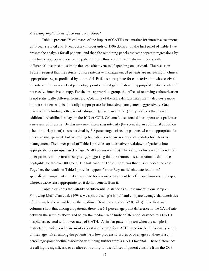
A. Testing Implications of the Basic Roy Model

Table 1 presents IV estimates of the impact of CATH (as a marker for intensive treatment)

on 1-year survival and 1-year costs (in thousands of 1996 dollars). In the first panel of Table 1 we

present the analysis for all patients, and then the remaining panels estimate separate regressions by

the clinical appropriateness of the patient. In the third column we instrument costs with

differential-distance to estimate the cost-effectiveness of spending on survival. The results in

Table 1 suggest that the returns to more intensive management of patients are increasing in clinical

appropriateness, as predicted by our model. Patients appropriate for catheterization who received

the intervention saw an 18.4 percentage point survival gain relative to appropriate patients who did

not receive intensive therapy. For the less appropriate group, the effect of receiving catheterization

is not statistically different from zero. Column 2 of the table demonstrates that it also costs more

to treat a patient who is clinically inappropriate for intensive management aggressively. One

reason of this finding is the risk of iatrogenic (physician induced) complications that require

additional rehabilitation days in the ICU or CCU. Column 3 uses total dollars spent on a patient as

a measure of intensity. By this measure, increasing intensity (by spending an additional $1000 on

a heart-attack patient) raises survival by 3.8 percentage points for patients who are appropriate for

intensive management, but by nothing for patients who are not good candidates for intensive

management. The lower panel of Table 1 provides an alternative breakdown of patients into

appropriateness groups based on age (65-80 versus over 80). Clinical guidelines recommend that

older patients not be treated surgically, suggesting that the returns to such treatment should be

negligible for the over 80 group. The last panel of Table 1 confirms that this is indeed the case.

Together, the results in Table 1 provide support for our Roy-model characterization of

specialization—patients most appropriate for intensive treatment benefit most from such therapy,

whereas those least appropriate for it do not benefit from it.

Table 2 explores the validity of differential distance as an instrument in our sample.

Following McClellan et al. (1994), we split the sample in half and compare average characteristics

of the sample above and below the median differential distance (-2.0 miles). The first two

columns show that among all patients, there is a 6.1 percentage point difference in the CATH rate

between the samples above and below the median, with higher differential distance to a CATH

hospital associated with lower rates of CATH. A similar pattern is seen when the sample is

restricted to patients who are most or least appropriate for CATH based on their propensity score

or their age. Even among the patients with low propensity scores or over age 80, there is a 3-4

percentage-point decline associated with being further from a CATH hospital. These differences

are all highly significant, even after controlling for the full set of patient controls from the CCP

13

(the first-stage F-statistics on differential distance are over 50 for all specifications reported in

Table 1).

The third and fourth columns of Table 2 report survival rates for patients above and below

the median differential distance. If differential distance is unrelated to patient mortality risk, then

these estimates can be combined with the difference in CATH rates from the first two columns to

form a simple Wald estimate of the effect of CATH on survival. Among all patients, there is a 0.9

percentage point decline in survival associated with being further from a CATH hospital,

suggesting that the intensive treatment associated with CATH leads to improved survival. The

Wald estimate suggests that CATH is associated with a 15 percentage-point improvement in

survival (.009 gain in survival / .061 increase in CATH), an estimate quite close to the 14.2

percent estimate from Table 1 that controlled for the full set of patient controls. The remaining

rows show results for other patient samples that are similarly consistent with the Table 1

estimates, with a larger association between differential distance and survival seen among patients

that are more appropriate for CATH and no relationship seen among patients that are less

appropriate for CATH. Given the similarity of the Wald estimates to IV estimates with a full set

of patient controls, it appears that differential distance is uncorrelated with observable differences

in mortality risk. The fifth and sixth columns show that, as expected, there is little difference in

the average 1-year predicted survival rate (from a logit of survival on the patient controls) for

patients above and below the median differential distance.

The final two columns of Table 2 compare average 30-day predicted CATH rate (the

propensity to get CATH) for only those patients getting CATH in the areas above and below

median differential distance. If the additional patients getting CATH in the low differential

distance sample were less appropriate for CATH, we would expect to see that the average patient

getting CATH in these areas would have a lower propensity. In contrast, we see little difference in

the sample that is nearer to a CATH hospital. Thus, it appears that differential distance is an

instrument that increases CATH rates among a sample of patients that is very similar (at least on

observable factors) to the average patient being treated. Therefore, it appears reasonable to

interpret the IV coefficients as estimates of the treatment effect in the treated population.

In the remaining tables we evaluate the between-area predictions of our model. We begin

with testing the simplest between-area implication: To be consistent with an economic model of

specialization, our theoretical model predicts that as areas increase their intensity the additional

patients receiving the intensive management should be less clinically appropriate for the

intervention. In contrast, a non-economic model would predict that intensive areas simply perform

more intensive treatments on all patients; there is no triage of patients into the treatment based on

their appropriateness. To test this insight we estimate:

14

(7) Appropriatenessij = µ0 + µ1 ln(Cath Rate)j + ei

The dependent variable is a measure of the appropriateness of a patient for cardiac cath (e.g., the

propensity score), and the equation is estimated at the patient level only for individuals receiving

CATH. The explanatory variable of interest is the natural logarithm of the risk-adjusted area

CATH rate. Following the logic of Gruber, Levine and Staiger (1999), the coefficient µ1 measures

the difference in mean Appropriateness between the average and the marginal patient receiving the

invasive treatment. If average appropriateness among patients getting CATH is declining as the

CATH rate rises (µ1<0), we infer that the marginal patient getting CATH was less appropriate than

the average patient (analogously to deriving marginal cost curves from average cost curves).

The results of estimating equation (7) are reported in Table 3. As the area’s intensity

increases, the marginal patient is 4.5 percentage points less likely to be appropriate for intensive

treatments. As a robustness check, we included two alternative measures of clinical

appropriateness: age and a measure of clinical ineligibility for CATH as defined by the American

College of Cardiologists (AHA) and the American Heart Association (AHA). Table 3 indicates

that by both measures, the marginal patient is significantly less likely to be appropriate for cardiac

catheterization.9

Figure 3 provides a graphical illustration of this relationship. For each of the 306 HRRs

we graph the average propensity to receive cardiac catheterization (amongst patients who actually

received it) against the log of the area risk-adjusted CATH rate. Using local-regression, we

estimated the relationship between the average propensity and the risk-adjusted CATH rate and

the slope of this line at each point (which we also smoothed). These estimates were then used to

plot average and marginal patient receiving treatment. As seen in the figure, average

appropriateness of patients getting CATH declines in more intensive areas. The average

appropriateness can decline only if the marginal patient is less appropriate— as the lower line in

Figure 3 indicates, the appropriateness of the marginal patient appears to be below the average

patient and also declines as areas become more surgically intensive.

B. Testing Implications of Productivity Spillovers

The empirical results in Tables 1-3 provide support for the basic assumptions of the Roy

model – that patients are sorted into surgery versus medical management based on the returns to

9 Both measures are included as covariates in our estimation of the empirical appropriateness for cardiac catheterization. As such, these results are not three separate confirmations of the same prediction. The ACC/AHA measures are based on an evaluation of the patients chart characteristics and classify each patient as being ideal, appropriate, and inappropriate for catheterization; see Scanlon et.al (1999) for details.

15

each type of treatment. The remaining tables focus on testing for the presence of productivity

spillovers. Table 4 tests the prediction that the quality of medical management is worse in areas

that are surgically intensive. To measure the extent of intensive treatment in an area, we use the

risk-adjusted 30-day CATH rate in each HRR. The risk-adjusted CATH rate reflects variation

across areas in the probability that observationally identical patients will receive CATH, and

therefore measures the productivity externality through its role of increasing the probability of

receiving the intensive treatment (see equation 2). To measure the quality of medical care in an

area, we use the risk-adjusted rate ate which patients received beta-blockers in the HRR. Use of

beta-blockers is a widely used marker for the quality of medical care. Not surprisingly, the risk-

adjusted CATH rate is positively correlated with other risk-adjusted rates of intensive surgical

treatment such as bypass (CABG) and angioplasty (PTCA). More importantly, the negative

correlation between the risk-adjusted CATH and beta-blocker rates supports the view that the

quality of medical management is worse in surgically intensive areas.

The remaining rows of Table 4 report the correlation between risk-adjusted CATH rates

and other area-level characteristics of interest. Risk-adjusted CATH rates are positively associated

with cardiovascular surgeons per capita (physicians who perform cardiac surgery), and the number

of CATH labs per capita. These correlations are consistent with the view that a higher level of

support services available in high-intensity areas may contribute to the externalities. The last three

rows of this table demonstrate, perhaps surprisingly, that risk-adjusted CATH rates are not

strongly associated with demographic characteristics of the HRR such as population, income, or

education.

A more fundamental implication of productivity spillovers is that the same patient will be

more likely to receive intensive treatment in an area where more patients receive this type of

treatment. This suggests that the characteristics of other patients in the population will influence

the treatment choice of an individual. Empirically, this implies that risk-adjusted CATH rates (the

HRR effect on CATH, holding individual patient characteristics constant) should be higher in

areas where the average patient is more appropriate for CATH. In the first column of Table 5 we

regress risk-adjusted CATH rates on the average propensity to get CATH in each HRR. The

coefficient is statistically significant and implies that for every 1 percentage point increase in the

expected CATH rate (based on patient characteristics), there is an additional 0.71 percentage point

increase in the area CATH rate because of spillovers. In the second column we control for area

demographics which could potentially confound this relationship, but they are insignificant and do

not materially change the coefficient. In the final two columns, we repeat this exercise using the

risk-adjusted beta-blocker rate as the dependent variable. The model implies that we should see

the opposite effect in these regressions, as the rise in CATH-appropriate patients exerts a negative

16

externality on the quality of medical care. The coefficient on the average propensity to get CATH

is negative and significant, implying that every 1 percentage-point increase in the expected CATH

rate reduces the use of beta blockers by 0.75 percentage points. This estimate is also robust to

controls for area demographics, although the percent of the population under age 65 and per capita

income both have independent significant effects on beta-blocker use.

A key implication of the productivity spillovers, which cannot be reconciled by other

models, is that the return to intensive management should be higher in high-intensity areas versus

low intensity ones. To test this prediction, we use our estimates of HRR level intensity from the

estimation of equation (6) to classify patients as being treated in high or low intensity regions (as

measured by whether the risk-adjusted CATH rates is above or below the median rate). In Table 6,

we report IV estimates of the effect of receiving intensive management within each of these two

groups. The results of this analysis are reported in a manner that mirrors the estimates in Table 1.

The survival returns to intensive management in intensive areas is roughly three times the return

observed in low intensity areas, while there is no statistically significant difference in the costs

associated with the different areas. As an alternative test, we should also find that those areas with

poor medical management have better outcomes from the use of intensive procedures. In the next

panel of Table 6, we classify patients into areas of differing intensity based on the area’s risk-

adjusted beta-blocker usage rates. High beta-blocker usage is an indicator of high quality medical

management, suggesting that these areas have specialized in medical management and therefore

should have a low return to intensive treatment. Once again, we note the dramatic degree to which

the predictions of area specialization are at work: The impact of CATH on survival is much

smaller in areas with good medical management.

Finally, Table 7 tests a unique implication of productivity spillovers: Patients most

appropriate for intensive treatments are better off being treated in high-intensity areas, while

patients who are least appropriate for intensive treatments should be worse off in such areas. To

test this prediction we split patients into 3 equal-sized groups of appropriateness for intensive

treatments. Within each group, we report the relationship between survival and the area CATH

rate in the first column. We also report the relationship between spending and the area rate in the

second column. The first panel of Table 7 replicates the central finding from the area-variations

literature—area intensity is associated with costs but not associated with improved outcomes

among patients as a whole. However, as the second panel demonstrates this finding masks

significant heterogeneity in the effect of intensive by patient appropriateness. Patients appropriate

for intensive managements clearly benefit from being treated in intensive areas. However, as the

productivity externality predicts, patients least appropriate for intensive treatments are harmed as a

result of being treated in intensive areas. The size of the negative externality is surprisingly

17

large—increasing area CATH intensity by ten percentage points (0.1) would reduce the survival of

patients least appropriate for CATH by 0.75 percentage points. This finding holds true (although

less significant) when we split the data by alternative indicators of appropriateness for intensive

treatment, including age and ACC/AHA guidelines.

Our model suggests that patients who are inappropriate for CATH are worse off in

intensive areas because (1) the quality of medical management in these areas is worse than in

other areas, and (2) few of these patients receive intensive treatment, even in the more intensive

areas. The last two columns of Table 7 explore these two dimensions of care directly by

estimating the relationship between area CATH intensity and the rate at which patients receive

beta blockers (as an indirect marker of quality of medical management) and CATH (as a direct

marker of intensive management). Beta-blocker use is lower among all patient groups in the high

intensity areas, suggesting that quality of medical management is generally poor in these areas. At

the same time, CATH rates among those patients least appropriate for CATH rise much less in

high intensity areas than for other patients. Thus, worse outcomes for this group appear to result

from worse medical management in areas with high CATH intensity, as our model predicts.

Medical practice guidelines recommend that nearly all patients receive beta blockers,

independent of whether they are treated intensively or non-intensively. Nevertheless, one might

be concerned that lower beta-blocker use in high CATH intensity areas was simply the mechanical

substitution of surgery for beta blockers among a subset of patients, rather than a broad indicator

of low quality medical management. Figure 4 provides two pieces of evidence against this

mechanical interpretation. This figure plots the percent of patients who receive beta-blockers

during hospitalization against patient appropriateness for catheterization (estimated by a running

regression) in HRRs with risk-adjusted CATH rates above and below the median. First, the use of

beta blockers is actually higher among patients that are more appropriate for CATH, which is the

opposite of the mechanical substitution explanation. Furthermore, we see that intensive areas are

less likely to provide beta-blockers to all patients (as was seen in Table 7), suggesting that these

areas provide poor quality medical management to all patients.

Finally, our analysis has assumed that productivity spillovers depend on the proportion of

patients receiving a given treatment, rather than the absolute number. Alternatively, productivity

spillovers could be more prevalent in larger areas; larger HRRs such as Los Angeles or Manhattan

may excel at both the intensive and non-intensive delivery of care. To explore this hypothesis

further, we estimate the relationship between alternative measures of HRR size and patient

survival in Table 8. We regress 1-year survival on patient risk-adjusters, the risk-adjusted CATH

rate and the log of the resident population (first 4 columns) and log of AMIs per hospital (last four

columns). Table 8 demonstrates that the size measures are largely insignificant—larger areas do

18

not result in improved survival. On the other hand, the “externality” (as measured by the HRR

CATH rate) is always protective of patients who are appropriate for CATH and harmful for

inappropriate patients.

V. Conclusion

A very simple equilibrium model of patient treatment choice with geographic productivity

spillovers appears to rationalize the main stylized facts concerning variation across areas in the use

of technologically intensive medical care. The model yields a range of additional empirical

implications, which we found uniform support for in our analysis of treatment for heart attacks.

Alternative models, such as those based on “flat-of-the-curve” medicine and supplier-induced

demand, have fundamentally different implications that are clearly rejected by the data. Thus,

there appears to be strong empirical support for the presence of productivity spillovers in medical

care.

Although knowledge spillovers are the most natural interpretation of our model and

empirical results, there are certainly other mechanisms that could generate similar spillovers. For

example, the spillovers may come from a form of network externality, in which specialization in a

given treatment results in better support services arising in the area (e.g. specialized surgical

centers, nursing staff, etc.). Alternatively, area specialization may attract physicians with a

comparative advantage in that specialty, thereby generating better outcomes within the narrow

specialty but worse outcomes more broadly. These models share the key feature that

specialization in one sector improves productivity in that sector while reducing productivity

elsewhere, thereby reinforcing the tendency to specialize. A careful analysis of the welfare

implications of our results will require knowledge of the underlying mechanism. Nevertheless, all

of these mechanisms generate similar empirical implications in our data.

The presence of productivity spillovers may justify a policy intervention to ameliorate the

deleterious effects of the externality. However, evaluating the welfare implications of any

proposed intervention is not a trivial exercise. Understanding what policy lever to push hinges

importantly on whether the variations observed in the data are the consequence of single or

multiple equilibria. With multiple equilibria we may be able to identify areas stuck in sub-optimal

equilibrium, and one-time interventions that “shock” the system to a different equilibrium would

be called for (for example, see O’Connor et al. (1996)). With single equilibrium, productivity

spillovers can generate either too much or too little intensive treatments, depending on the size of

the externalities and the distribution of patients in the area. Thus, from a policy perspective, the

evidence to date has little to say about whether there is any reason to reduce the variation across

19

areas in the use of technologically intensive treatments or, if so, what would be the appropriate

policy response.

Our results also raise important questions about what can be learned from randomized

controlled trials in medicine. While randomized trials are considered the gold standard for

determining the effectiveness of a given medical treatment, they are designed to provide a partial-

equilibrium estimate of the treatment effect in a well-defined population. But with productivity

spillovers, the general equilibrium effect of adopting a new treatment could be smaller or larger

than the partial equilibrium estimate of treatment effectiveness, because of the negative externality

imposed on patients who are more appropriate for an alternative treatment and the positive

externality on patients who are more appropriate for the new treatment. This general-equilibrium

effect is not identified in a typical randomized trial, but could potentially be estimated in a trial

that randomized across areas rather than individuals. In addition, the effectiveness of the treatment

depends on where the trial is conducted (just as our IV estimates depended on intensity in the

area): Surgical interventions may perform poorly in an area that specializes in medical

management of its patients and perform well in a more surgically intensive area. As such the

external validity of a randomized trial is compromised.

The implications of our findings go well beyond the treatment of heart attacks. To the

extent that productivity spillovers are a common feature of many sectors, our results provide

compelling evidence that such spillovers are an important feature of geographic specialization.

Moreover, our results provide some of the first direct evidence of the negative externalities

imposed on a subset of the population because of equilibrium pressures towards specialization.

Such negative externalities are a central component of arguments for government intervention.

Finally, our model has interesting empirical implications when applied to the more general

question of human capital externalities. For example, our model would suggest that people living

in areas with higher ability populations would be more likely (holding ability constant) to go to

college, the return to going to college in these areas would be higher, but wages of low ability

people in these areas would be lower. In principal, these are all testable implications.

20

Data Appendix I. Construction of Hospital Referral Regions. Hospital Referral Regions are constructed using a two part algorithm. Step 1: All acute care hospitals in the 50 states and the District of Columbia were identified from the American Hospital Association Annual Survey of Hospitals and the Medicare Provider of Services files and assigned to a location within a town or city. The list of towns or cities with at least one acute care hospital (N=3,953) defined the maximum number of possible Hospital Service Areas (HAS). Second, all 1992 and 1993 acute care hospitalizations of the Medicare population were analyzed according to ZIP Code to determine the proportion of residents' hospital stays that occurred in each of the 3,953 candidate HSAs. ZIP Codes were initially assigned to the HSA where the greatest proportion (plurality) of residents were hospitalized. Approximately 500 of the candidate HSAs did not qualify as independent HSAs because the plurality of patients resident in those HSAs were hospitalized in other HSAs. The third step required visual examination of the ZIP Codes used to define each HSA. Maps of ZIP Code boundaries were made using files obtained from Geographic Data Technologies (GDT) and each HSA's component ZIP Codes were examined. In order to achieve contiguity of the component ZIP Codes for each HSA, "island" ZIP Codes were reassigned to the enclosing HSA, and/or HSAs were grouped into larger HSAs. This process resulted in the identification of 3,436 HSAs, ranging in total 1996 population from 604 (Turtle Lake, North Dakota) to 3,067,356 (Houston) in the 1999 edition of the Atlas. Intuitively, one may think of HSAs as representing the geographic level at which “front end” services such as diagnoses are received. Step II: Hospital service areas make clear the patterns of use of local hospitals. A significant proportion of care, however, is provided by referral hospitals that serve a larger region. Hospital referral regions were defined in the Dartmouth Atlas by documenting where patients were referred for major cardiovascular surgical procedures and for neurosurgery. Each hospital service area was examined to determine where most of its residents went for these services. The result was the aggregation of the 3,436 hospital service areas into 306 hospital referral regions that were named for the hospital service area most often used by residents of the region. Thus if a Medicare enrollee living in Hartford, CT were admitted to a hospital in Boston, MA, the utilization would be attributed to Hartford, and not to Boston. This assignment avoids the serious shortcoming of unusually high utilization rates in large referral centers such as Boston or Rochester, MN. II. Construction of CCP Estimation Sample: The CCP used bills submitted by acute care hospitals (UB-92 claims form data) and contained in the Medicare National Claims History File to identify all Medicare discharges with an International Classification of Diseases, Ninth Revision, Clinical Modification (ICD-9-CM) principal diagnosis of 410 (myocardial infarction), excluding those with a fifth digit of 2, which designates a subsequent episode of care. The study randomly sampled all Medicare beneficiaries with acute myocardial infarction in 50 states between February 1994 and July 1995, and in the remaining 5 states between August and November, 1995 (Alabama, Connecticut, Iowa, and Wisconsin) or April and November 1995 (Minnesota); for details see O’Connor et.al (1999). The Claims History File does not reliably include bills for all of the approximately 12% of Medicare beneficiaries insured through managed care risk contracts, but the sample was representative of the Medicare fee-for-service (FFS) patient population in the United States in the mid-1990s. After sampling, the CCP collected hospital charts for each patient and sent these to a study center where trained chart abstracters abstracted clinical data. Abstracted information included elements of the medical history, physical examination, and data from laboratory and diagnostic testing, in addition to documentation of administered treatments. The CCP monitored the reliability of the data by monthly random reabstractions. Details of data collection and quality control have been reported

21

previously in Marciniak et.al (1998). Finally, the CCP supplemented the abstracted clinical data with diagnosis and procedure codes extracted from Medicare billing records and dates of death from the Medicare Enrollment Database. For our analyses, we delete patients who were transferred from another hospital, nursing home or emergency room since these patients may already have received care that would be unmeasured in the CCP. We transformed continuous physiologic variables into categorical variables (e.g., systolic BP < 100 mm Hg or > 100 mm Hg, creatinine <1.5, 1.5-2.0 or >2.0 mg/dL) and included dummy variables for missing data. We used date of death to identify patients who did or did not survive through each of three time points: 1-day, 30-days, and 1-year after the AMI. For all patients, we identified whether they received each of 6 treatments during the acute hospitalization: reperfusion (defined as either thrombolysis or PCI within 12 hours of arrival at the hospital), aspirin during hospitalization, aspirin at discharge, beta-blockers at discharge, ACE inhibitors at discharge, smoking cessation counseling, and each of 3 treatments within 30-days of the AMI: cardiac catheterization, PCI, or CABG. We used the ACC/AHA guidelines for coronary angiography to identify patients who were ideal (Class I), uncertain (Class II), or inappropriate (Class III) for angiography; these details are provided in Scanlon et.al (1999). For each AMI patient we computed Medicare Part A and Part B costs within 1 year by weighting all Diagnosis Related Groups (DRGs) and Relative Value Units (RVUs) nationally. This measure of costs abstracts from the geographic price adjustment in the Medicare program. III. Construction of clinical appropriateness index, HRR cathetherization rates, and HRR beta-blocker rates. To compute this index we estimate a logistic regression model for the probability of receiving cardiac catheterization within 30 days of the heart-attack. We estimate:

Pr(Cardiac Cathij)= F(θ0 + θj + XiΦ) Pr(Beta Blockersij)= F(θ0 + Πj + XiΦ)

Fitted values from this regression, Pr(Cath|X), are used as an empirical measure clinical appropriateness for cardiac catheterization. The HRR fixed effects for the use of cardiac catheterization and beta-blockers are obtained as θj, and Πj respectively. Note that these fixed-effects are not used to obtain our empirical measure of appropriateness for cardiac catheterization. Included in this model are the following risk-adjusters: Age, Race, Sex (full interactions) previous revascularization (1=y) hx old mi (1=y) hx chf (1=y) history of dementia hx diabetes (1=y) hx hypertension (1=y) hx leukemia (1=y) hx ef <= 40 (1=y) hx metastatic ca (1=y) hx non-metastatic ca (1=y) hx pvd (1=y) hx copd (1=y) hx angina (ref=no)

hx angina missing (ref=no) hx terminal illness (1=y) current smoker atrial fibrillation on admission cpr on presentation indicator mi = anterior indicator mi = inferior indicator mi = other heart block on admission chf on presentation hypotensive on admission hypotensive missing shock on presentation peak ck missing

peak ck gt 1000 non-ambulatory (ref=independent) ambulatory with assistance ambulatory status missing albumin low(ref>=3.0) albumin missing(ref>=3.0) bilirubin high(ref<1.2) bilirubin missing(ref<1.2) creat 1.5-<2.0(ref=<1.5) creat >=2.0(ref=<1.5) creat missing(ref=<1.5) hematocrit low(ref=>30) hematocrit missing(ref=>30) ideal for CATH (ACC/AHA criteria)

22

References Acemoglu, Daron and Joshua Angrist. “How Large are Human Capital Externalities? Evidence from

Compulsory Schooling Laws,” in Ben S. Bernake and Kenneth Rogoff, Eds., NBER Macroeconomics Annual Volume 15 (Cambridge, MA: MIT Press) 2000: 9-59.

Arthur, W. B. “Competing technologies, increasing returns, and lock-in by historical events,” Economic Journal 99, 1989: 116-131.

Andersen HR, Nielsen TT, Rasmussen K, et al. “A comparison of coronary angioplasty with fibrinolytic therapy in acute myocardial infarction,” New England Journal of Medicine 349, 2003:733-742.

Beck, Christine A., John Penrod, Theresa W. Gyorkos, Stan Shapiro, Louise Pilote “Does Aggressive Care Following Acute Myocardial Infarction Reduce Mortality? Analysis with Instrumental Variables to Compare Effectiveness in Canadian and United States Patient Populations,” Health Services Research 38(6), 2003: 1423-40.

Coleman, J.S., Katz, E., and Menzel, H. “The Diffusion of an Innovation Among Physicians” Sociometry 20(4), December 1957: 253-270

Cutler, David and Mark McClellan “Productivity Change in Health Care,” American Economic Review 2001a: 281-286.

Cutler, David and Mark McClellan “Is Technological Change in Medicine Worth It?” Health Affairs, 20(5) 2001b: 11-29.

Cutler, David. “Equality, Efficiency and Market Fundamentals: The Dynamics of International Medical Care Reform,” Journal of Economic Literature XL, September 2002: 881-906.

Baicker, Katherine and Amitabh Chandra, “Medicare Spending, The Physician Workforce, and The Quality Of Health Care Received By Medicare Beneficiaries.” Health Affairs, April 2004a: 184-97.

Baicker, Katherine and Amitabh Chandra, “The Productivity of Physician Specialization: Evidence from the Medicare Program,” American Economic Review 90(2), May 2004b: 333-38.

Becker, Gary and Kevin Murphy, “The Division of Labor, Coordination Costs, and Knowledge.” Quarterly Journal of Economics 107(4), November 1992: 1137-1160.

Chassin MR, Brook RH, Park RE, et al. Variations in the use of medical and surgical services by the Medicare population. New England Journal of Medicine 1986; 314:285-290.

Fisher, Elliott, et al. "Hospital Readmission Rates for Cohorts of Medicare Beneficiaries in Boston and New Haven." New England Journal of Medicine 1994; 331: 989-95.

Fisher, Elliott, et al., “The Implications Of Regional Variations In Medicare Spending. Part 1: The Content, Quality, And Accessibility Of Care.” Annals of Internal Medicine, February 18, 2003, 138(4): 273-87.

Fisher, Elliott, et al., “The implications of regional variations in Medicare spending. Part 2: Health outcomes and satisfaction with care.” Annals of Internal Medicine, February 18, 2003, 138(4): 288-98.

Glover, Allison F., "The Incidence of Tonsillectomy in School Children,” Proceedings of the Royal Society of Medicine 31, 1938: 1219-1236.

Goolsbee, Austan and Peter Klenow. “Evidence on Learning and Network Externalities in the Diffusion of Home Computers,” Journal of Law & Economics 45, October 2002: 317-344.

23

Gruber, Jonathan, Phillip B. Levine, and Douglas Staiger. “Abortion Legalization and Child Living Circumstances: Who is the Marginal Child?” Quarterly Journal of Economics, 1999: 263-292.

Heckman, James J. and Bo Honore. “The Empirical Content of the Roy Model,” Econometrica, 58(5) Sept. 1990: 1121-49.

Jaffe, Adam, Trajtenberg, Manuel and Henderson Rebecca. “Geographic Location of Knowledge Spillovers as Evidenced by Patent Citations,” Quarterly Journal of Economics 108(3), August 1993: 577-98.

Jacobs, Alice K. “Primary Angioplasty for Acute Myocardial Infarction -- Is It Worth the Wait?” New England Journal of Medicine 2003, 349: 798-800.

Jencks SF, et al., “Quality of Medical Care Delivered to Medicare Beneficiaries.” Journal of the American Medical Association, 284(13), October 4, 2000:

Katz M. L., and Shapiro C. "Network externalities, competition, and compatibility," American Economic Review 75, 1985: 424-440.

Katz, M. L., and Shapiro, C. “Technology adoption in the presence of network externalities,” Journal of Political Economy 94, 1986: 822-841.

Keeley EC, Boura JA, Grines CL. “Primary angioplasty versus intravenous thrombolytic therapy for acute myocardial infarction: a quantitative review of 23 randomised trials,” Lancet 361, 2003:13-20.

Leape, Lucian L., R.E. Park, D.H. Solomon et al., “Does Inappropriate Use Explain Small Area Variations in the Use of Health Care Services,” Journal of the American Medical Association 1990, 263(5):669-672.

Lomas, J., M. Enkin, G.M. Anderson, W.J. Hannah, E. Vayda, and J. Singer, ”Opinion Leaders vs. Audit and feedback to implement practice guidelines: delivery after previous cesarean section,” Journal of the American Medical Association 1991, 265:2202-2207.

McClellan, Mark, B.J. McNeil and J.P. Newhouse. “Does more intensive treatment of acute myocardial infarction reduce mortality?” Journal of the American Medical Association September 1994, 272(11): 859-66,.

McClellan, Mark and J.P. Newhouse “The marginal cost-effectiveness of medical technology: a panel instrumental-variables approach,” Journal of Econometrics 77(1) March 1997: 39-64,.

Marshall, Alfred. Principles of Economics. (New York NY: Macmillan), 1890.

Marciniak TA, Ellerbeck EF, Radford MJ, et al. “Improving the quality of care for Medicare patients with acute myocardial infarction: results from the Cooperative Cardiovascular Project.” Journal of the American Medical Association 1998; 279:1351-1357.

Moretti, Enrico. “Human Capital Externalities in Cities,” National Bureau of Economic Research Working Paper 9641, April 2003.

Moretti, Enrico. “Worker’s Education, Spillovers, and Productivity: Evidence from Plant Level Production Functions,” American Economic Review 94(3), June 2004a: 656-91.

Moretti, Enrico. “Estimating the Social Return to Higher Education: Evidence from Longitudinal and Repeated Cross-Sectional Data,” Journal of Econometrics 121, 2004b: 175-212.

O'Connor Gerald T., et. al “A regional intervention to improve the hospital mortality associated with coronary artery bypass graft surgery. The Northern New England Cardiovascular Disease Study Group.”Journal of the American Medical Association 1996; 275(11):841-6.

24

O'Connor, Gerald T., Quinton, H. B., Traven, N. D., Ramunno, L. D., Dodds, T. A., Marciniak, T. A., Wennberg, J. E. “Geographic Variation in the Treatment of Acute Myocardial Infarction: The Cooperative Cardiovascular Project,” Journal of the American Medical Association 1999 281: 627-633

Phelps, C.E. “Information Diffusion and Best Practice Adoption,” in Handbook of Health Economics, Volume 1, edited by AJ Culyer and JP Newhouse, Elsevier Science B.V., 2000: 224 -264.

Pilote L, McClellan M, Saynina O, Lavoie F. “Cardiac procedures use and outcomes in elderly patients with acute myocardial infarction in the United States and Canada, 1988-1994,” Medical Care 41(7), 2003:813-822.

Scanlon PJ, Faxon DP, Audet AM, et al. “ACC/AHA guidelines for coronary angiography. A report of the American College of Cardiology/American Heart Association Task Force on practice guidelines (Committee on Coronary Angiography). Developed in collaboration with the Society for Cardiac Angiography and Interventions.” Journal of the American College of Cardiology. 1999; 33(6):1756-824.

Soumerai, Stephen B., et al. “Effect of Local Medical Opinion Leaders on Quality of Care for Acute Myocardial Infarction: A Randomized Controlled Trial,” Journal of the American Medical Association 1998 279: 1358-1363.

Tu, Jack V., Pashos, Chris L., Naylor, C. David, Chen, Erluo, Normand, Sharon-Lise, Newhouse, Joseph P., McNeil, Barbara J. “Use of Cardiac Procedures and Outcomes in Elderly Patients with Myocardial Infarction in the United States and Canada,” New England Journal of Medicine 336, 1997: 1500-1505

Wennberg, John and MM Cooper, Eds. The Quality of Medical Care in the United States: A Report on the Medicare Program, The Dartmouth Atlas of Health Care 1999 (Chicago: American Health Association, 1999).

Wennberg, David E., JD Birkmeyer, Eds. The Dartmouth Atlas of Cardiovascular Health Care. (Chicago: American Hospital Publishing, Inc, 2000).

Zucker, Lynne G., Darby, Michael R., and Brewer, Marilynn B. “Intellectual Human Capital and the Birth of U.S. Technology Enterprises,” American Economic Review 88(1), March 1998: 290-306.

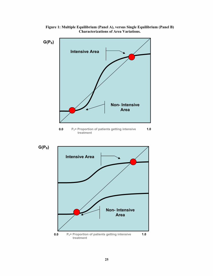
25

Figure 1: Multiple Equilibrium (Panel A), versus Single Equilibrium (Panel B)

Characterizations of Area Variations.

0.0 1.0

Ps= Proportion of patients getting intensive treatment

G(PS)

Intensive Area

Non- Intensive Area

0.0 1.0

Ps= Proportion of patients getting intensive treatment

G(PS)

Intensive Area

Non- Intensive Area

26

Figure 2: Graphical Illustration of Specialization with Productivity Spillovers

Panel A describes the relationship between two alternative ways to treat patients within an area. The survival production possibilities frontier describes the best treatment for a patient of given clinical appropriateness. The model predicts that the returns to intensive management are increasing in patients’ appropriateness for such interventions. Panel B contrasts the care across two areas that differ in their surgical intensity. The productivity spillover results in patients appropriate for intensive management being better off in the surgically intensive areas, whereas patients appropriate for non-intensive management being worse off in such areas. See Section II of text for details and formal model.

Clinical Appropriateness for Intensive Management

Survival

Treat Intensively

Treat Non-Intensively

Prediction: Return is HIGHER for those who are more appropriate for intensive management.

Survival if Treated Intensively

Survival if Treated Non-intensively

Clinical Appropriateness for Intensive Management

Prediction: Treated surgically in intensive area, but medically in less-intensive area

Prediction: Least Appropriate are WORSE OFF in an intensive area

Prediction: Most Appropriate are BETTER OFF in an intensive area Intensive Area

Non- Intensive Area

Survival

27

Figure 3: Relation Between Average Patient and Marginal Patient Receiving Cardiac Catheterization

For each of the 306 HRRs we graph the average propensity to receive cardiac catheterization (amongst patients who actually received it) against the log of the area risk-adjusted CATH rate. Using local-regression, we estimated the relationship between the average propensity and the risk-adjusted CATH rate and the slope of this line at each point. These estimates were then used to plot average (upper line) and marginal patient (lower line and estimated as the local difference in the average) receiving treatment.

Ave

rage

pro

pens

ity to

get

CA

THam

ong

patie

nts

getti

ng C

ATH

HRR risk-adjusted cath rate (log scale)

Average patient getting CATH Marginal patient getting CATH HRR data point

.2 .3 .4 .5 .6 .7

.55

.6

.65

.7

.75

28

Figure 4: Percent of Patients Getting Beta Blockers by Patient Propensity to Get Cath In HRRs With Low (Top Line) and High (Bottom Line) Risk-Adjusted Cath Rate

%

get

ting

beta

blo

cker

s

Cath propensity

0 .2 .4 .6 .8 1

.2

.3

.4

.5

.6

.7

This figure plots the percent of patients who receive beta-blockers during hospitalization against patient appropriateness for catheterization (estimated by a local regression) in HRRs with risk-adjusted CATH rates above and below the median.

29

Table 1: Instrumental Variable Estimates of Intensive Management and Spending on 1 Year Survival by Clinical Appropriateness of Patient

IV Estimates of Impact of CATH: Impact of $1000:

Sample: on 1-Year Survival

on 1-year Cost ($1000s)

on 1-year Survival

1. All patients 0.142 9.086 0.016 (n=129,895) (0.036) (1.810) (0.005) 2.By CATH propensity a. Above the Median 0.184 4.793 0.038 (n=64,799) (0.034) (1.997) (0.017)

b. Below the Median 0.035 17.183 0.002 (n=65,096) (0.083) (3.204) (0.005)

Difference: 0.149 -12.39 0.036 (0.090) (3.775) (0.018) 3. By age a. 65-80 0.171 6.993 0.024 (n=89,947) (0.037) (1.993) (0.009) b. Over 80 0.016 16.026 0.001 (n=39,948) (0.108) (2.967) (0.007)

Difference: 0.155 -9.033 0.023 (0.114) (3.574) (0.011)

Notes: CATH propensity is an empirical measure of patient appropriateness for intensive treatments. We define this measure by using fitted values from a logit model of the receipt of cardiac catheterization on all the CCP risk-adjusters. Differential-distance (measured as the distance between the patient’s zip-code of residence and the nearest catheterization hospital minus the distance to the nearest hospital) is the instrument. Each model includes all the CCP risk-adjusters and the standard errors are clustered at the level of each HRR.

30

Table 2: Relationship Between Differential-Distance and Probability of Catheterization and Survival, and Differential-Distance and Observable Characteristics

30-day CATH rate

1-year Survival

1-year Predicted Survival

30-day predicted CATH rate for patients getting CATH

DD Below Median

DD Above Median

DD Below Median

DD Above Median

DD Below Median

DD Above Median

DD Below Median

DD Above Median

Sample: All patients 48.9% 42.8% 67.6% 66.7% 67.5% 67.2% 63.3% 63.2% (n=129,997) By CATH propensity Above the Median 74.0% 67.1% 84.6% 83.8% 83.4% 83.5% 72.6% 72.6% (n=64,733)

Below the Median 22.9% 19.5% 50.1% 50.4% 51.1% 51.6% 32.3% 32.5% (n=65,244) By age 65-80 61.1% 54.9% 74.3% 73.5% 73.9% 73.9% 67.4% 67.3% (n=90,016) Over 80 20.3% 16.5% 52.1% 52.1% 52.6% 52.7% 34.6% 34.1% (n=39,961)

Notes: CATH propensity is an empirical measure of patient appropriateness for intensive treatments. We define this measure by using fitted values from a logit model of the receipt of cardiac catheterization on all the CCP risk-adjusters. Differential-distance (measured as the distance between the patient’s zip-code of residence and the nearest catheterization hospital minus the distance to the nearest hospital) is the instrument. Each model includes all the CCP risk-adjusters and the standard errors are clustered at the level of each HRR.

31

Table 3: Relationship between the Average and Marginal Patient Receiving Cardiac Catheterization

Characteristic of average patient getting CATH across all areas

Patient Characteristic

Difference Between average patient and marginal patient getting CATH in higher-CATH HRRs

1. CATH propensity 0.633 -0.045 (0.002) (0.008) 2. Over age 80 0.125 0.063 (0.002) (0.012)

0.028 0.010 3. Not eligible for CATH using ACC/AHA guidelines (0.001) (0.003)

Notes: CATH propensity is an empirical measure of patient appropriateness for intensive treatments. We define this measure by using fitted values from a logit model of the receipt of cardiac catheterization on all the CCP risk-adjusters. Sample is restricted to patients receiving cardiac catheterization within 30 days of an AMI. ACC/AHA guidelines reflect a binary variable assigned to each patient in the CCP that measures whether the patient is ideal, appropriate, or not eligible for catheterization based on chart-review.

32

Table 4: Correlation of HRR Level Measures of Intensive Treatment, Medical Management, Support of Medical Treatment and Demographic Characteristics

Correlation 10th 90th with HRR HRR indicator Mean SD percentile percentile CATH rate

Measures of intensive treatment Risk-adjusted 30-day CATH rate 46.3% 9.1% 34.5% 58.3% 1.00 Risk-adjusted 30-day PTCA rate 17.7% 5.1% 11.3% 23.6% 0.81 Risk-adjusted 30-day CABG rate 13.4% 2.9% 10.2% 16.9% 0.51 Risk-adjusted 12-hour PTCA rate 2.7% 2.6% 0.6% 5.8% 0.52 Measures of Quality of medical management Risk-adjusted β-blocker rate 45.6% 9.5% 34.2% 58.3% -0.31 Support for intensive treatment Cardiovascular Surgeons per 100,000 1.06 0.27 0.70 1.40 0.33 Cath Labs per 10,000 2.40 0.76 1.50 3.30 0.39 Demographic characteristics log of resident population 13.96 0.89 12.72 15.18 -0.05 log of per capita income 9.55 0.20 9.31 9.85 0.02 Percent College graduates 19.3% 5.5% 13.1% 26.6% -0.05

Notes: HRR surgical and medical intensity rates are computed as the risk-adjusted fixed effects from a patient level regression the receipt of CATH or beta-blockers on HRR fixed effects and CCP risk-adjusters. CATH propensity is an empirical measure of patient appropriateness for intensive treatments. We define this measure by using fitted values from a logit model of the receipt of cardiac catheterization on all the CCP risk-adjusters.

33

Table 5: Relationship between HRR Patient Characteristics and HRR Treatment

HRR Level Dependent Variables

HRR-Level Independent Variables:

Risk-adjusted30-day CATH rate

Risk-adjusted30-day CATH rate

Risk-adjusted Beta Blocker Rate

Risk-adjustedBeta Blocker Rate

Average propensity to get CATH 0.707 0.761 -0.753 -0.590 (0.248) (0.239) (0.306) (0.205) Percent under age 65 0.253 -0.534 (0.193) (0.199) log of resident population -0.006 -0.009 (0.008) (0.009) log of per capita income 0.031 0.209 (0.034) (0.031) R-squared 0.04 0.05 0.04 0.21 N 303 303 303 303

Notes: HRR surgical and medical intensity rates are computed as the risk-adjusted fixed effects from a patient level regression the receipt of CATH or beta-blockers on HRR fixed effects and CCP risk-adjusters. CATH propensity is an empirical measure of patient appropriateness for intensive treatments. We define this measure by using fitted values from a logit model of the receipt of cardiac catheterization on all the CCP risk-adjusters.

34

Table 6: Instrumental Variable Estimates of Intensive Management and Spending on Survival, by Surgical Intensity of Hospital Referral Region

Impact of $1000:

Sample:on 1-Year Survival

on 1-year Cost ($1000s)

on 1-year Survival

1. By HRR risk-adjusted CATH rate

a. Above the Median 0.256 6.691 0.038 (n=63,771) (0.061) (3.510) (0.021)

b. Below the Median 0.09 9.835 0.009 (n=66,124) (0.059) (3.155) (0.007)

Difference: 0.166 -3.144 0.029(0.085) (4.720) (0.022)

2. By HRR risk-adjusted β-blocker rate

a. Below the Median 0.189 6.33 0.03 (n=64,862) (0.050) (2.434) (0.013)

b. Above the Median 0.071 11.003 0.006 (n=65,033) (0.048) (2.550) (0.005)

Difference: 0.118 -4.673 0.024

IV Estimates of

Impact of CATH:

Notes: HRR intensity rates are computed as the risk-adjusted fixed effects from a patient level regression the receipt of CATH or beta-blockers on HRR fixed effects and CCP risk-adjusters. Differential-distance (measured as the distance between the patient’s zip-code of residence and the nearest catheterization hospital minus the distance to the nearest hospital) is the instrument. Each model includes all the CCP risk-adjusters and the standard errors are clustered at the level of each HRR.

35

Table 7: Relationship Between HRR Catheterization Rate, Survival and Costs, by Clinical Appropriateness for Intensive Management

OLS Estimates of the Relationship Between HRR Risk-Adjusted CATH Rate and:

Sample: 1-Year Survival

1-year Cost ($1000s)

Beta Blocker in Hospital

Catheterization within 30 days

1. All patients 0.007 8.093 -0.28 0.702 (n=138,873) (0.019) (1.410) (0.073) (0.004) 2. By CATH propensity a. Top Tercile 0.052 10.012 -0.366 0.802 (n=46,287) (0.019) (1.439) (0.073) (0.032)

b. Middle Tercile 0.03 11.154 -0.271 0.906 (n=46,295) (0.030) (1.784) (0.082) (0.021)

c. Bottom Tercile -0.075 2.763 -0.209 0.369 (n=46,291) (0.028) (1.612) (0.073) (0.021) Difference (Top-Bottom): 0.127 7.249 -0.157 0.433 (0.034) (2.161) (0.103) (0.038) 3. By age a. 65-80 0.023 9.616 -0.311 0.775 (n=96,093) (0.021) (1.448) (0.072) (0.012)

b. Over 80 -0.031 4.738 -0.215 0.531 (n=42,780) (0.028) (1.603) (0.080) (0.022) Difference (Top-Bottom): 0.054 4.878 -0.096 0.244 (0.035) (2.160) (0.108) (0.025) 4. By AHA/ACC criterion a. Ideal 0.027 9.845 -0.302 0.769 (n=89,569) (0.023) (1.599) (0.076) (0.010)

b. Appropriate -0.002 6.174 -0.282 0.752 (n=31,800) (0.024) (1.537) (0.080) (0.026)

c. Not appropriate -0.08 2.958 -0.177 0.264 (n=17,504) (0.040) (1.511) (0.065) (0.021) Difference (Top-Bottom): 0.107 6.887 -0.125 0.505 (0.046) (2.200) (0.100) (0.023)

Notes: CATH propensity is an empirical measure of patient appropriateness for intensive treatments. We define this measure by using fitted values from a logit model of the receipt of cardiac catheterization on all the CCP risk-adjusters. HRR surgical and medical intensity rates are computed as the risk-adjusted fixed effects from a patient level regression the receipt of CATH or beta-blockers on HRR fixed effects and CCP risk-adjusters.

36

Table 8: Relationship between Survival and alternative measures of HRR size, by clinical appropriateness of patient

By CATH propensity By CATH propensity HRR-Level Independent Variables:

All patients

Top Tercile

Middle Tercile

Bottom Tercile

All patients

Top Tercile

Middle Tercile

Bottom Tercile

Risk-adjusted CATH rate 0.006 0.052 0.031 -0.077 0.008 0.053 0.031 -0.075 (0.019) (0.019) (0.030) (0.028) (0.019) (0.019) (0.030) (0.028) log of resident population -0.002 -0.001 0.002 -0.007 (0.002) (0.002) (0.003) (0.003) log of AMIs per hospital 0.005 0.014 0.006 -0.007 (0.004) (0.005) (0.007) (0.006) N 138,873 46,287 46,295 46,291 138,873 46,287 46,295 46,291

Notes: CATH propensity is an empirical measure of patient appropriateness for intensive treatments. We define this measure by using fitted values from a logit model of the receipt of cardiac catheterization on all the CCP risk-adjusters. HRR surgical and medical intensity rates are computed as the risk-adjusted fixed effects from a patient level regression the receipt of CATH or beta-blockers on HRR fixed effects and CCP risk-adjusters.