NBER WORKING PAPER SERIES

RANK-ORDER TOURNAMENTS ASOPTIMUM LABOR CONTRACTS

Edward P. Lazear

Sherwin Rosen

Working Paper No. 401

NATIONAL BUREAU OF ECONOMIC RESEARCH1050 Massachusetts Avenue

Cambridge MA 02138

November 1979

We are indebted to Merton Miller for helpful comments on afirst draft. The research was supported in part by theNational Science Foundation. The research reported hereis part of the NBER's research program in Labor Studies.Any opinions expressed are those of the authors and notthose of the National Bureau of Economic Research.

NBER Working Paper 401November 1979

Rank-Order Tournaments as Optimum Labor Contracts

ABSTRACT

It is sometimes suggested that compensation varies across individualsmuch more dramatically than would be expected by looking at variations intheir marginal products. This paper argues that a compensation schemebased on an individual's relative position within the firm rather than hisabsolute level of output will, under certain circumstances, be the preferredand natural outcome of a competitive economy. Differences in the level ofoutput between individuals may be quite small, yet optimal "prizes" areselected in a way that induces workers to allocate their effort and invest­ment activities efficiently.

In particular, by compensating workers on the basis of their relativeposition in the firm, one can produce the same incentive structure for risk­neutral workers that the optimal and efficient pie~e rate produces. It mightbe less costly however, to observe relative position than to measure thelevel of each worker's output directly. This results in the payment ofprizes, wages which for some workers greatly exceeds their presumed marginalproducts. When risk aversion is introduced, the prize salary structure nolonger duplicates the allocation of resources induced by the optimal piecerate. For activities which have a high degree of inherent riskiness, pay­ment based on relative position will dominate.

Finally, when workers are allowed to be heterogeneous, an importantresult is obtained. Competitive contests which pay workers on the basis oftheir relative position will not, in general, sort workers in a way whichyields an efficient allocation of resources. In particular, low qualityworkers will attempt to contaminate a firm comprised of high quality workers,even in the absence of production complimentarities. This suggests thathigh quality firms will use non-price techniques to allocate jobs to appli­cants.

Edward P. LazearSherwin RosenDepartment of EconomicsUniversity of Chicago1126 E. 59th StreetChicago, II 60637

312/753-4525312/753-4503

I. INTRODUCTION

It is a familiar proposition in labor economics that under competitive

conditions workers are paid the value of their marginal products. In order

for this statement to be meaningful, it is apparent (see Alchian and

Demsetz, 1972) that some mechanism exist for ascertaining and monitoring

productivity. If inexpensive reliable monitors are available, the optimal

compensation method is a periodic wage that pays on the basis of observed

input. However, when the firm cannot monitor input as closely as the worker

can, compensation based on input that the firm actually observes invites

shirking by workers and may be inefficient. In these cases, the situation

can be improved if rewards are based on output, so long as that is more

easily observed by both parties. It is true that compensation geared to

, input is generally superior to that based on output when monitoring costs

are negligible, because workers must bear more risk in an incentive contract

than in a wage contract, creating gains from trade if the firm is less risk­

averse than are its employees. Nevertheless, when monitoring is not free,

the gain in efficiency from output or incentive payments may outweigh the

loss of utility due to additional risk-bearing of workers.

A wide variety of incentive payment schemes are used in practice and

one of them, simple piece rates, has been extensively analyzed (e.g., see

Cheung (1969), Stiglitz (1975), Mirrlees (1976)). In this paper we consider

another type of incentive payment, namely contest and prizes, that has not

been analyzed very much, yet which seem to be prevalent, either implicitly

or explicitly, in many labor contracts. The main difference between

prizes and other types of incentive compensation is that in a

2

contest earnings depend on rank order among a group of workers, whereas

piece rates typically are paid on the basis of individual performance.1

The prototype contest is the tennis match, where winning and losing prizes

are fixed in advance, independently of each player's performance in that

particular contest.

The analysis of alternative compensation schemes is related to the

problem of moral hazard and providing appropriate incentives for eliciting

effort and investment when information is costly and monitoring costs are

asymmetric. Each type of compensation method is characterized by certain

parameters, such as the piece rate, the prize structure and so forth. For

each scheme we seek the values of the parameters that maximize utility of

workers, subject to a zero profit constraint for competitive firms. For

familiar reasons, the scheme that actually emerges in competitive markets

achieves the unconditional maximum utility of workers among the set of

conditional maximums. Two dimensions of incentives need to be distinguished:

one is investment or skill acquisition prior to the time a work activity is

entered and the other is the effort expended, after skills have been

acquired, in a given work situation or play of the game. In this work we

concentrate on the first and ignore the second. The emphasis on prior

investment lends itself most readily to an interpretation of earnings

prospects over the whole life cycle, or lifetime rather than annual earnings.

Section II demonstrates that two-player tournaments achieve the same

allocation of resources as piece rates when workers are risk-neutral.

Therefore, choice between the two forms of payment depends on costs of

assessing rank rather than individual performance. These issues are

important for the structure of executive pay. Section III extends these

3

results to N-player tournaments; sequential tournaments with eliminations,

which give rise to skewed realized reward structures; and to problems where

rank rather than total output is valued by consumers. Section IV shows the

very surprising result that tournaments can be the social optimum contract

when workers are risk-averse. This is applied to a problem originally

formulated by Friedman (1951) on the relation between skewness in the

overall earnings distribution and workers' preferences for lotteries.

Section V discusses problems of adverse selection in tournaments in the

presence of population heterogeneity and asymmetric information, and the

economic structure of handicapping systems when these differences are known

to everyone.

II. PIECE RATES AND TOURNAMENTS WITH RISK-NEUTRALITY

A. Piece Rates

Consider the simplest linear production structure in which worker j

produces (lifetime) output qj according to

where ~ is the worker's precommitted choice of investment in the activity

(a measure of skill) and € is a random or luck component drawn out of a

known distribution with 2E(€.) = o.

JProduction requires only labor and

production risk is completely diversifiable for firms, so entrepreneurs act

as expected value maximizers, or as if they were risk-neutral. Notice that

this production structure, which is maintained throughout, specifies that a

worker's product is a random variable, but that the mean of the probability

4

distribution can be affected by the worker's own actions. The incentive

mechanism is designed to elicit the optimum value of ~, or to choose the

"correct" distribution. Analysis of the case where workers can also affect

variance is left for some other occasion.

The piece rate solution is very simple to analyze in this case. Let

the piece rate be r. Ignoring discounting, the worker's net income is

rq - ~(~), where C(jJ) is the cost of producing skill level jJ, with

C' and C" > O.. Risk-neutral workers choose jJ to maximize

which, for given r, implies C'(jJ) = r: investment equates marginal cost

and marginal return. Let the firm sell the output on a competitive market

at price Then expected profit is

E(Vq - rq) = (V - r)jJ

so entry and competition for workers bids up the piece rate to r = V.

This implies, in conjunction with the worker's investment criteria, that

(2) C'(jJ) = V

Therefore the marginal cost of investment equals its social return, the

4standard result that piece rates are efficient.

B•. Rank-Order Tournaments

Now consider a two-player tournament in which the rules of the game

specify a fixed prize WI to the winner and a fixed prize W2 to the loser.

Production of each player, j and k, follows (1), with €:.,i=j,k~

5

independently and identically distributed, and E(E:.) = 01.

and

Th~ winner is determined by the largest drawing of q. The contest is

rank-order because the margin of winning does not affect earnings.

Contestants precommit their investment strategy knowing the rules of the

game and the prizes and do not communicate or collude during the investment

period. We seek the competitive equilibrium prize structure (W1,WZ) .

. Consider the contestant's problem, assuming that both have the same

costs of investment C(~), so that their behavior is identical. A

contestant's expected utility (wealth) is

P(W l - C(~» + (1 - P)(WZ - C(~»

(3) = PWI + (1 - P)WZ - C(~)

where P is the probability of winning. The probability that j wins is

P = prob(qj > qk) = prob(~j - ~ > E:k - E:j

)

(4) - prob(~j - ~k > ~) = G(~j - ~)

where ~ = E:k

- E:j

• ~ ~ g(~), G(o)

= zcrZ (because E: and E:E: j k

is the cdf of g(~), E(~) = 0 and

are i.i.d.). Each player chooses ~i

to maximize (3), which requires, assuming interior solutions,

(WI - WZ)ap c' (~ ) = 0---a~. i

1.

(5) i = j,k

(WI - WZ)aZp _

C"(~.) < 0Z 1.

a~i

We adopt the Nash-Cournot assumptions that each player optimizes

against the optimum investment of his opponent.(or he plays against the

market over which he has no influence). This is perhaps justified

6

because investment is precommitted, each player is a small part of the

market and does not know the identity of his opponent at the time investment

decisions are made. Thus j takes ~ as given in determining his

investment and conversely for k. It then follows from (4) that, for player

j

which upon substitution into (5) yields j's reaction function

Player k's

reversed.

reaction function looks the same except with ~j and

The symmetry of (6) implies that when the Nash solution exists

~j = ~k and P = G(O) =~. However, it is not necessarily true that there

is a solution because with arbitrary density functions the objective function

(3) may not be concave in the relevant range. 5 It is possible to show that

a solution exists provided that cr2 is sufficiently large, i.e., contestse:

are feasible only when the variance of chance is large enough. This result

accords with intuition and is in the spirit of the old saying that a

(sufficient) difference of opinion is necessary for a horse race. Technical

details are slightly tedious and therefore are relegated to an appendix.

Existence of an equilibrium is assumed in all that follows.

Substituting ~j = ~k at the Nash equilibrium equation (6) reduces to

(7) i = j ,k

so each player's investment depends on the spread between winning and losing

prizes. The levels of the prizes only influence the decision to enter the

7

game and the players' expected rent if entry is profitable. The condition

for entry is that maximum expected utility be nonnegative. With P = ~

equation (3) becomes

which simply says that expected winnings at the best investment strategy

must be at least as large as opportunity cost if workers are to enter the

tournament.

The risk-neutral firm is more passive. Its actual gross receipts are

(qj + qk)'V and its ~osts are the total prize money WI + WZ• Competition

for labor bids up the purse to the point where expected total receipts equal

costs, or WI + Wz = (~j + ~k) ·V.

the zero profit condition reduces to

But since ~ = ~ = ~j kin equilibrium,

Therefore the expected value of product equals the expected prize in

equilibrium. Substituting (8) into the worker's utility function (3) with

P = ~ in equilibrium, the worker's expected utility at the optimum

investment strategy is

(9) V~ - C(~).

The equilibrium prize structure selects WI and W2 to maximize (9) or

(10) i = 1,2

and the marginal cost of investment equals its social marginal return,

v = C'(~), in the tournament as well as the piece rate. So competitive

tournaments, like piece rates, are efficient and both result in exactly

the same allocation of resources.

8

To summarize the analysis, the problem for the firm is to choose a

prize structure (W1,W2) that maximizes profits. The decision by

individuals to invest in skill or effort (~) depends upon the spread

between winning and losing. As the spread increases, the incentive to

devote additional resources to improving one's probability of winning

increases. The firm would like to increase the spread and thereby induce

higher productivity "play" (which increases the firm's revenue). However,

as the spread increases contestants invest more, but their costs are

increased as well. The latter is what limits the spread. A firm offering

too large a spread induces excessive investment. A competing firm can

attract all the workers by·decreasing the spread, because it lowers workers'

costs by more than it lowers expected earnings and therefore raises expected

utility. If the marginal cost of skill acquisition is increasing, there is

a unique equilibrium spread between the prizes that maximizes expected

utility.

Some further manipulation of the equilibrium conditions yields an

interesting interpretation in terms of the theory of agency (see Ross (1972),

Becker and Stigler (1974) and Harris and Raviv (1978». Solve (7) and (8)

for WI and W2 to obtain

WI = V~ + C'(~)/2g(O) = V~ + V/2g(O)

(11)

Wz = V~ - C'(~)/2g(O) = V~ - V/2g(O)

The second equality follows from V = C'(~). Now think of the term

C'(~)/2g(O) or V/Zg(O) in (11) as an entrance fee or bond that is

p~ted by each player. The winning and losing prizes payoff the marginal

9

value product plus or minus the entrance fee. That is, the players receive

their marginal product combined with a fair winner-take-all gamble over the

total entrance fees or bonds. The appropriate social investment incentives

are given by each contestant's attempt to win the gamble. This contrasts

with the main agency result, where the bond is returned to each worker

after a satisfactory performance has been observed. There the incentive

mechanism works through the employee's attempts to work hard enough to

recoup his own bond. Here it works through the attempts to win the contest.

Let us conclude this part of the discussion with some comparative

statics, all of.which follow from the marginal conditions (10) and the

worker's investment decision (7). These two imply also that

We first see what happens when the distribution of luck is changed.

From (7), all that matters about the random variables is the value of the

distribution of ~ at ~ = 0, or g(O). It is clear, however, from the

definition ~= Ek - E. that a reduction in the variance of luck 02

J E

concentrates the pdf of ~ around zero so that g(O) increases. For

example, if E is normal then g(O) = 1/21 'IT02 and ag(O)/aOE

< O. YetE

condition (10) shows that the optimal investment is independent of the

higher moments of the distribution of chance for risk-neutral workers:

marginal cost equals marginal return irrespective of g(~) so long as

E(~) = O. Therefore a reduction in luck does not change the quality of

the contestants. It does reduce the spread (WI - W2 ), from (12).

Equation (11) shows also that WI falls and W2 rises, i.e., the total

entrance fees decline and the size of the gamble falls. The reason is

10

that a given incremental investment buys each player a smaller incremental

probability when luck is more important. The stakes must therefore increase

to give contestants the proper marginal incentives to invest. This implies

that among risk-neutral workers the optimal prizes are closer together in

occupations that are inherently less riskY~ Note that paying by the piece

gives a similar result.

There are only two other exogenous factors in this problem: parameters

of the cost function, C(]..I), and V. From condit.ion (12) the spread is

independent of costs for a given value of V. However, anything that

increases marginal costs must reduce investment since V = C'(]..l). From (11),

this condition implies no reduction in the entrance fee, which remains at

V/Zg(O), but a reduction in the "certain income" V']..I. Both prizes are

reduced by the same amount because the lower total product cannot support

the same total prize money.7 An increase in V with given costs raises

investment since its value has increased, from (10). The incentive to

invest more is signalled by an increase in the spread, from (lZ). Greater

total productivity also supports a larger total purse WI + WZ' Equation

(11) implies that W1 must increase, but Wz need not rise. The entrance

fee and magnitude of the gamble are incr.,ased in any case, which is another

way of saying that investment incentives rise.

Finally, there is an important practical implication of these results.

While it remains true from the zero profit condition (8) that ex ante

expected wages equal expected marginal product in a tournament, the actual

realized earnings definitely do not equal marginal productivity in either

an ex ante or ex post sense. Consider ex ante first. Since ]..lj = ]..Ik = ']..I,

expected marginal products are equal. So long as W1 > Wz' which it must

11

to induce any investment, the payment that j receives never equals the

payment that k receives. It is impossible that the prize is equal to

ex ante marginal product, because ex ante marginal products are equal.

It is equally obvious that wages are not equal to ex post marginal products.

Actual marginal product for j is Vqj rather than V~j. But qj is a

random variable, the value of which is not known until after the game is

played~ while Wi and W2 · are fixed in advance. Only under the rarest

coincidence would Wi = vqj and W2 = Vqk. Therefore, wages do not equal

ex post marginal products.

C. Comparisons

All compensation schemes can be viewed as transforms of the distribution

of productivity into the distribution of earnings. The piece rate of

Section II.A is a linear transform and apart from a change in the mean and

a change in scale, the earnings distribution absolutely follows the

distribution of output. The tournament in Section II.B is an entirely

different animal. It is a distinctly nonlinear transformation that converts

the continuous distribution of productivity into a discrete binomial

distribution of earnings. In spite of this difference, we have shown that

a competitive prize-tournament structure duplicates the allocation of

resources achieved by a piece rate structure, when workers are risk-neutral.

This is clear from examination of conditions (2) and (10). In both cases

the fundamental marginal condition is the same: V = ct(~) so investment

is the same. The reason for this is that risk-neutral workers only care

about the first moment of the earnings distribution and in both cases that

is given by V~ - C(~), where ~ is determined by (2) or (10). Even

Ii

though the higher moments differ, those differences do not affect expected

ut~lity or wealth. In Section IV we analyze cases where workers are risk­

averse. There, preferences for higher order moments in addition to the

mean serve to break the tie between the two schemes on the grounds of

tastes alone.

Nevertheless, we believe that even in the risk-neutral setting there

are important factors that influence the choice between the two. Chief

among them are possible differences in costs of information. If rank is

more easily observed than each individual's level of output, tournaments

dominate piece rates. On the other hand, occupations in which an

individual's output level is easily observed would have no particular

preference for a prize scheme. For example, salesmen whose output is

easily observed are paid by piece rates, whereas many business executives,

whose output is much more difficult to observe, engage in contests.

Consider the salary structure for executives. It appears as though

the salary of, say, the vice-president of a particular corporation is

substantially below that of the president of that same corporation. Yet

presidents are often chosen from the ranks of vice-presidents. On the day

that a given individual is promoted from vice-president to president, his

salary may triple. It is difficult to argue that his skills have tripled

in that one-day period, presenting difficulties for standard theory, where

supply factors should keep wages in those two occupations approximately

equal. It is not a puzzle, however, when interpreted in the context of a

prize. If the president of a corporation is viewed as the winner of a

match and as such receives the higher prize, WI' then that wage payment

is settled upon not only because it reflects his current productivity as

13

president, but rather because it induces that individual and all other

individuals to perform appropriately when they are in more junior positions.

This interpretation suggests that presidents of large corporations do not

necessarily earn high wages because they are more productive as presidents,

but because this particular type of payment 'structure makes them more

productive over their entire working life. A contest provides the proper

incentives for skill acquisition prior to coming into the position~

III. RISK-NEUTRALITY: SOME EXTENSIONS

This section extends the analysis to N players and also discusses some

aspects of sequential contests.

A. Several Contestants

It is easy to show that the formal equivalence between piece rates and

tournaments is not an artifact of two-player games, when all players are

risk-neutral and have identical costs. players and

prizes, W. for i th place.~

worker's expected utility is

N(13) EPiW

i- C(~)

Let there be N

The probability of i th place is P. ,~

N

so a

Since the players are identical, the Nash solution, if it exists, implies

Pi = l/N for all i and for all players. Therefore (13) becomes, in

equilibrium,

(14) (EW.)/N - C(~)~

14

However, for zero expected profit, the total purse must be exactly supportedN

by expected revenues. Expected revenue is E(6Vq.) = NV~, so competitive~

equilibrium requires 6W. = NV~.~

Substituting into (14), each worker acts

to maximize V~ - C(~). That is, ~ is chosen to satisfy V = C'(~) just

as in the two-player case. Therefore a tournament is efficient independent

of the number of players.

There is a curious feature of the N-player case that only first and

last place prizes are uniquely determined in competitive equilibrium. This

is sufficiently nonobvious that it is worth discussing, but requires a few

details and is therefore relegated to appendix 2. This indeterminacy is a

feature of the risk neutral case and vanishes when risk aversion is intro-

duced.

B. Sequential Contests

This section considers a few aspects of sequential games. Before

doing so, it is necessary to clarify a possible point of confusion between

what might be labeled repetitive and sequential contests.

1. Repetitive games

The point at issue concerns the proper interpretation of the stochastic

term E in the output technology q = jl + E. As stated at the outset,

we think of as investment and of q as lifetime output. There-

fore E must be interpreted as "lifetime luck"; or alternatively as

a drawing out of a known distribution of life-persistent person effects or

15

ability whose realization is unknown to all agents at the time investment

decisions and contracts are drawn up. On this interpretation, € is

revealed only very slowly, and strictly speaking in the .formal model above,

at the end of the lifetime. Clearly, there is only a single period or one-

time tournament in a whole lifetime, though the "period" is a long one to

be sure.

In repetitive play one might think of a series of, say, annual contests.

This stands in the same relation to a single lifetime contest as a compound

lottery does to a simple lottery. Let annual output be written

Suppose now that €t is i.i.d.--qt = Jl + €t' where t is a year index.

2 2E(€t) = 0, E(€t) = cr and E(€t€s) = 0 for t +s . In this case has

the interpretation of "pure luck." In this case also, however, annual risk

is diversifiable by each worker over his lifetime, e.g., by using a saving

account, since a good outcome in a given year is likely to be offset by an

equally poor outcome in some other year. The point is that with sufficient

repetition and independent error all risk would be diversified away,

for basically the same reasons that the sample standard deviation of the mean

of a distribution shrinks to zero as the sample size increases. Incottle could

be made constant over the lifetime and the tournament structure would unravel.

Consequently, in order for a tournament to make sense there must be

some risk that is nondiversifiable by the worker and that is revealed only

9relatively slowly. Put in another way, € is the remaining element of

chance after all independent components have been diversified through

repetition. The simplest error structure consistent with this requirement

is a variance-component specification €it = 0i + nit' where i refers to

persons and t to years. Clearly, we have nothing to say about risk that

the worker can diversify himself.

16

2. Sequential games: information and skew

The main interest of sequential contests is their possible use in

gaining information about the undiversifiable chance component in lifetime

productivity. The analogy with sequential statistical analysis is suggestive

of how € (or 0 in the variance-component) comes to be revealed. We

cannot do justice to this complicated problem here and the following brief

ff . 10comments must su ~ce.

Contests with eliminations give rise to a skewed income distribution.

Consider sequential two-player games starting with N players. A winner

is selected through a series of paired contests, "quarter-finals," "semi-

finals," and "finals." The first round consists of N/2 two-person matches:

N/2 players lose, earning W21 . N/2 win, receiving WII plus the

opportunity to advance to the next round. In the second round N/4 are

losers and N/4 are winners. So N/4 end up with WII + W22 and N/4

get WII + WI2 plus the opportunity to advance to the next round. The

final distribution of income has N/2 with W21 ; N/4 with Wll+ W

22;

ZN/8 with Wil + WI2 + W

23, etc., and the winner, with L W as income,

t=1 Itwhere Z = in N/in 2. This distribution has positive skew.

A plausible story can be told which yields sequential contests and

skew. Returning to the point that rank may be less costly to determine

than individual outputs, suppose further that it is cheaper to determine

relative position in a two-person game than in a multi-person game. Let

0i be an unobserved ability component for player i, with neither

contestants nor firms taking this into account when selecting an optimal ~

because it is unobserved at the time of investment. Then

where n is pure luck and tthrefers to the t

17

contest. If we want to select the players with the largest ~ + ° it also

pays to have only winners play winners, since

Therefore a sequential elimination tournament may be a cost-efficient way

of selecting the best person.ll

Information about prior outcomes influences wage rates and prizes in

sequential games. To illustrate, let production take place in two periods

and consider a two-player contest played in period 1 only. The winner

receives (W11 ,WI2 ) in periods 1 and 2 respectively and the loser gets

(WZ1 ,WZ2)' Ignoring discounting for simplicity, lifetime income is

WI = W11 + W12 for the winner and Wz = WZ1 + W22 for the loser. Each

player chooses ~ before the game is played to maximize expected wealth

PW1 + (1 - P)W2 C(~) and the Nash solution is identical to Section II.B:

C'(~) = g(O) (WI - W2). The budget constraint is only slightly altered to

WI + Wz = 4V~, so in competitive equilibrium WI and Wz are basically

the same as before, though twice as large because production takes place

over two periods instead of one.12

If workers are not bound to the same firm over their lifetime then

competition would bid up the second period wage of the winner to the

expected value of the second or largest order statistic:

W12 :I E(Vqj2 1j wins) = V~ + VE(oj Iqj 1 > qkl) , where qil is first-period

production and qi2 is second-period production of player i. The reason

is that a competing firm, knowing a game had been played, could infer the

second-period conditional expectation of the winner's product simply by

knowing his identity. The same logic implies WZ2 = E(vqjZlj loses) =

V~ + E(ojlqjl < qkl). If the firm organizing the contest attempted to

18

ensure that the winner stayed by paying more than E(VQj2 !j wins), it

would have to pay less than the conditional expectation to the loser.

Competition for losers would make the firm unactuarial in period 2 and

invite bankruptcy. With W12 and W22 fixed by their conditional

expectation, Wll and W21 are determined to be consistent with the

competitive game equilibrium comditions on gross wealth WI and W2 , the

firm is actuarially balanced period by period and it makes no difference

if the players depart or not in period 2. One can even imagine the

existence of firms whose major activity is running contests among young

workers (period i) that provide sorting and information services for other

firms for older workers (period 2), minor leagues in a sense. This is

essentially financed by the workers themselves in the manner of the

entrance fees discussed in Section II. This places restrictions on the

shape of the "age-earnings" profile, but there remains an element of in-

determinacy to the prize or wage in each period, though not to wea.lth,

and W 132'

C. Rank-Order Objective Functions

It is of some interest to note that the fundamental solution to the

tournament prize structure survives a broad class of alternative specifi-

cations of the revenue function. Consider a horse race. The criterion

v . (Uj + Uk) assumes that gate receipts are proportional to the total or

average speed in the race. It may be that spectators also care about rank

as well as overall speed. Let Qi be the expected value of the speed of

19

the i th place horse (an order statistic). If spectator's willingness

to pay depends on the expected quality of the winning horse, revenue is

instead of So long as win and place prizes

so gate receipts also dependis the cdf ofthenof

and W2 are the stakes, contestants still behave exactly as in Section II:

~ is the same for both and depends on the spread. If F(e) is the cdf

F2(Q -~)

1

on the spread through its influence on the distribution of the winner's

expected speed. The competitive prize structure still maximizes contestants'

expected utility but the zero profit constraint is somewhat altered from the

above. However, only the details differ: The equilibrium spread solves the

maximum problem and the prize levels satisfy the constraint. Similar

considerations apply if revenue depends on Q1 and Q2 so that spectators

care about expected speeds of both ranks and on the closeness of the contest.

Notice that since the revenue function always involves ~,there always

exists an alternative piece rate scheme: For example, each horse could be

paid in proportion to its speed. Therefore virtually the same issues of

comparison arise as those considered above: Even if revenue depends on rank

the optimum compensation method need not depend on rank.

As an historical note, one of the few papers we have been able to find

on the prize structure in tournaments is by Sir Francis Galton (1902).15

Galton considered a race with n-contestants where a fixed sum was to be

divided among the first two places. With prizes W1 and W2 Galton

proposed the following division on strictly a priori grounds

20

That is, the ratio of first to second prize stands in the same relation as

th~ corresponding expected rank-order differences over third place. This

criterion is roughly related to expected relative outcomes or productivity.

Galton's work is an important paper in statistics but is less interesting

to economists because it does not take account of a contestant's incentive to

run fast. His contest is a random draw of a sample of size n from a fixed

population. By contrast, the crucial aspect of our work is in allowing the

prize structure to change the population distributions through incentives to

invest. The population distributions are therefore endogenous in our model

but exogenous in his model. Nonetheless, Galton went on to show the

remarkable result that (Ql - Q3)/(Q2 - Q3) is approximately 3.0 independent

of n when the parent distribution is normal. Therefore his criterion leads

to a highly skewed prize structure. This result would perhaps be less

surprising today, given what is known about the characteristic skew of

extreme value distributions, yet it does roughly concur with the prize

structures commonly observed in sports activities such as tennis and horse

racing. Skew is not necessarily an implication of a single n-player contest

in our model, though it is not inconsistent with it. We believe, however,

that skewed prizes in each play of a repetitive game structure may be a

strong implication of the incentive to elicit effort in each round and that

dimension has been ignored here.

21

IV. OPTIMAL PRIZE STRUCTURE WITH RISK-AVERSION

In the previous section, we obtained the surprising result that

contests and piece-rate compensation schemes yield identical and efficient

allocations of resources. In this section, we allow for risk-aversion of

contestants and show that the choice of compensation scheme is no longer

indeterminate. Even when costs of ascertaining output are zero, the

piece-rate scheme tends to dominate for distributions of € with low

variance, while prizes tend to dominate for high variance distributions.

The reason is roughly as follows: In a piece-rate scheme, players are

paid a fixed sum (to be determined optimally) plus some proportion of their

output. The higher is the variance in chance, €j' the higher will tend

to be the variance in income (although this can be offset by reducing the

variable and increasing the fixed part of the payment). A prize structure

truncates the extremes of the distribution by converting it to a binomial.

However, the necessity of a positive spread in the prize structure implies

that there must be some variance in income. For small 2a ,€

it appears as

though the variance introduced by the requisite spread exceeds that which

results from paying by the piece. But as 2a gets large, higher expected€

utility is produced by fixing maximum gain and loss in advance with prizes

than by taking one's chance and allowing €j to affect wages strongly.

The fixed component would have to be so high relative to the variable

piece component in the piece rate that investment incentives are too small

and prizes dominate.

22

A. Optimum Linear Piece Rate 16

The piece-rate scheme analyzed pays workers a fixed amount, I, plus

rq, where r is piece rate per unit of output. The problem for the firmJ

is to pick an r, I vector that maximizes workers' expected utility

(15) max{E(U) = maxfU(y)8(y)dy}l,r

where

(16)

y:: I + rq - C(1l )

- I + rll + r8 - C(ll)

and 8(y) is the pdf of y. Since V~ is expected revenue from a worker

and I + r~ is expected wage payments, the zero profit market constraint is

(17) V~ := I + r~ .

The worker's problem is to choose ~ to maximize expected utility, given

r· and r. If € '" f (€) , the worker's problem is

Max E(U) := fU(I + r~ + r€ - C(~»f(€)d€ •~

The first-order condition is

aEa~U) = f[U'(y)](r - C'(~»f(€)d€ := 0 ,

which conveniently factors so that

(18) r = C'(~) .

Condition (18) is identical to the risk-neutral case, and it should be.

Investing in ~ gives a certain return of r; the error, €, is

23

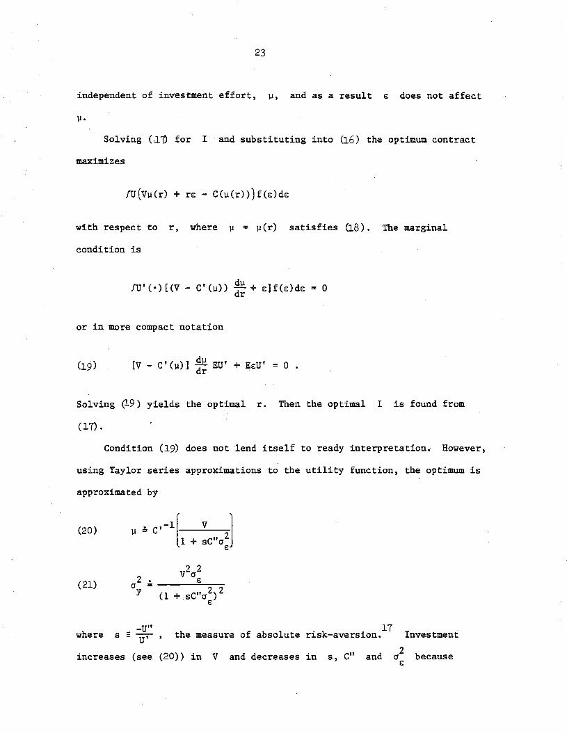
independent of investment effort, ~, and as a result e does not affect

Solving (,1'0 for I and substituting into u.6) the optimum contract

maximizes

with respect to r, where ~ = ~(r) satisfies u.8). The marginal

condition is

d~!U'(·)[(V - C'(~» dr + e]f(e)de = 0

or in more compact notation

[v - C'(~)] d~ EU' + EeU' = 0 .dr

Solving ~9) yields the optimal r. Then the optimal I is found from

(17) •

Condition (19) does not lend itself to ready interpretation. However,

using Taylor series approximations to the utility function, the optimum is

approximated by

(20)

(21)

h f b 1 . k . 17t e measure 0 a so ute r1S -averS10n.where_ -U"

s = U'

increases (see (20» in V and decreases in s, C" and2

cre

Investment

because

24

all these changes imply corresponding changes in the marginal piece rate

r which influences investment through condition (18). The same changes

in V, sand C" have corresponding effects on the variance of income

(see (21» but an increase in 2(J

€:can actually reduce variance if 2

(J€:

is

large because it reduces r and increases I.

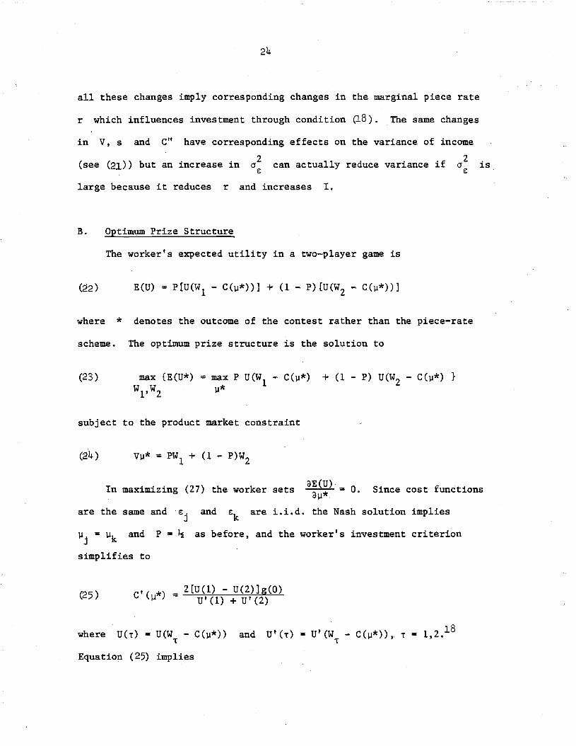
B. Optimum Prize Structure

The worker's expected utility in a two-player game is

(~2) E(U) = P[U(W1 - C(p*»] + (1- P)[U(W2 - C(p*»]

where * denotes the outcome of the contest rather than the piece-rate

scheme. The optimum prize structure is the solution to

(23) max P U(W1 - C(p*)p*

+ (1 - P) U(W2

- C(p*) }

subject to the product market constraint

Vp* = PW + (1 - P)W1 2

In maximizing (27) the worker sets oE(U) = 0oll* . Since cost functions

are the same and and €k are i.i.d. the Nash solution implies

Pj = Pk and P = ~ as before, and the worker's investment criterion

simplifies to

(25 ) C'(].l*) = 2[U(I) - U(2)]g(0)U' (1) + U' (2)

where U(.) = U(W - C(ll*»• and = U' (W - C(ll*»,' • = 1,2.18

•Equation (25) implies

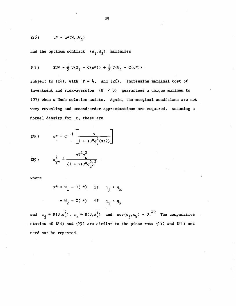
25

and the optimum contract (W1,WZ) maximizes

(27) 1 1EU* = 2" U(W1 - C(lJ*)) + 2" U(WZ - C(lJ*)) .

subject to (24), with P =~, and (26). Increasing marginal cost of

investment and risk-aversion (U" < 0) guarantees a unique maximum to

(27) when a Nash solution exists. Again, the marginal conditions are not

very revealing and second-order approximations are required. Assuming a

normal density for €, these are

z •(Jy* =

where

= W - C(Il*)Z

if

if

statics of (28) and (29) are similar

and

need not be repeated.

and19

cov(€j'€k) = O. The comparative

to the piece rate (20) and (21) and

26

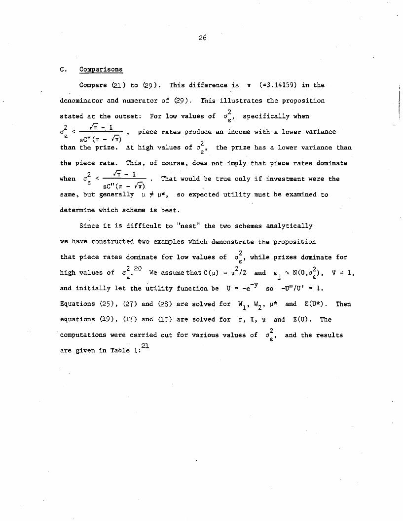
C. Comparisons

Compare (21) to (29). This difference is rr (=3.14159) in the

denominator and numerator of ~9). This illustrates the proposition

piece rates produce an income with a lower variance

2At high values of cr, the prize has a lower variance thane

than

stated at the outset:

2 .;; - 1(j < ----"---

e: sC"(rr _ /;)the prize.

For low values of 2cr ,e: specifically when

the piece rate. This, of course, does not imply that piece rates dominate

when 2 1;- 1 That would be true only if investment were thecr <e: sC" ('IT - /;)

same, but generally fl :f: fl*, so expected utility must be examined to

determine which scheme is best.

Since it is difficult to "nest" the two schemes analytically

we have constructed two examples which demonstrate the proposition

that piece rates dominate for low values of

and initially let the utility function be

while prizes dominate for

and v = 1,2e. 'V N(O,cr ),J e

-U" /U' = 1.soU = -e-y

2cr ,e

2= fl /2We assume that C(fl)Z 20

cr •e

high values of

Equations (25) , (27) and (28) are solved for WI' Wz' fl* and E(U*). Then

equations (19) , (17) and (15 ) are solved for r, I, fl and E(U). The

computations were carried for various values of 2 and the resultsout cr ,e:21

are given in Table 1:

27

Table 1

Constant Absolute Risk-Aversion

2)l* E(U) - E(U*)(J )l

-f..

.5 .667 1.03 .2751.5 .. 40 .678 .0882.5 .285 .567 .0293.0 .25 .532 .0123.5 .222 .505 -.00086.5 .133 .413 -.0418.0 .117 .395 -.051

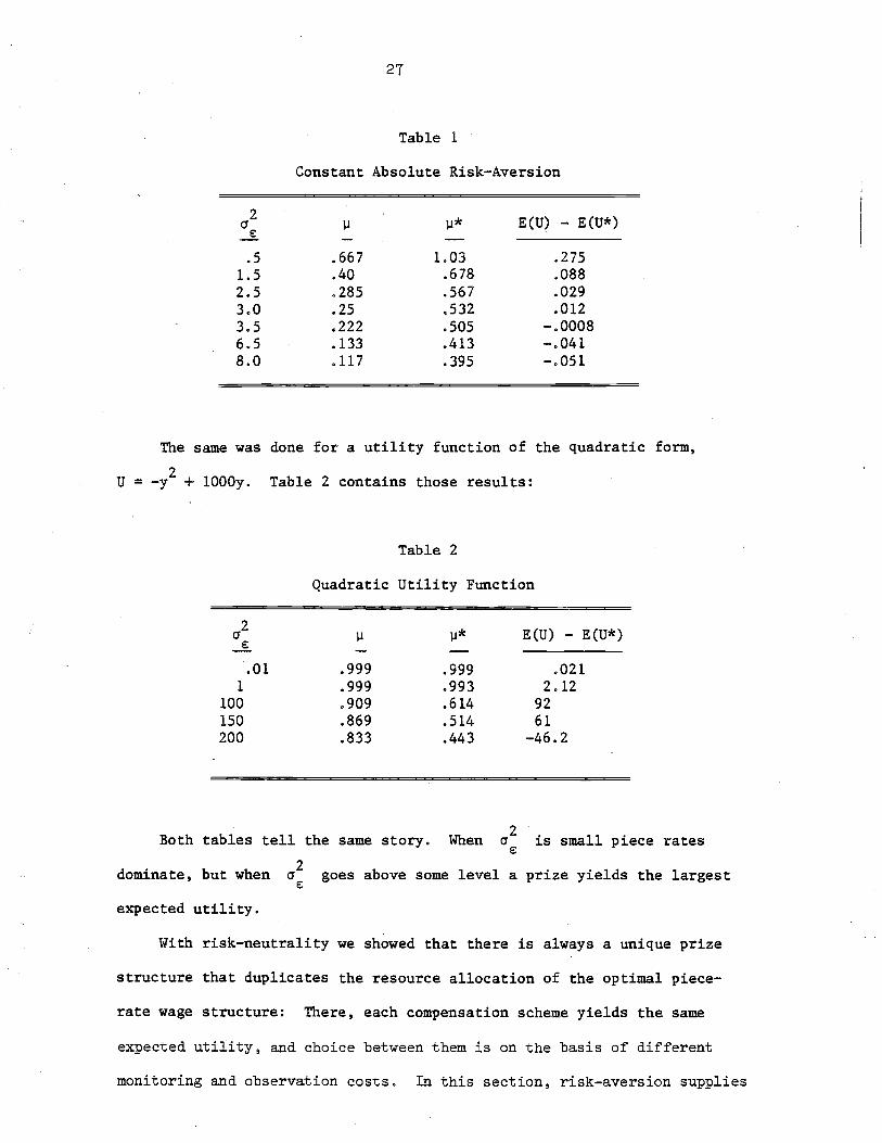
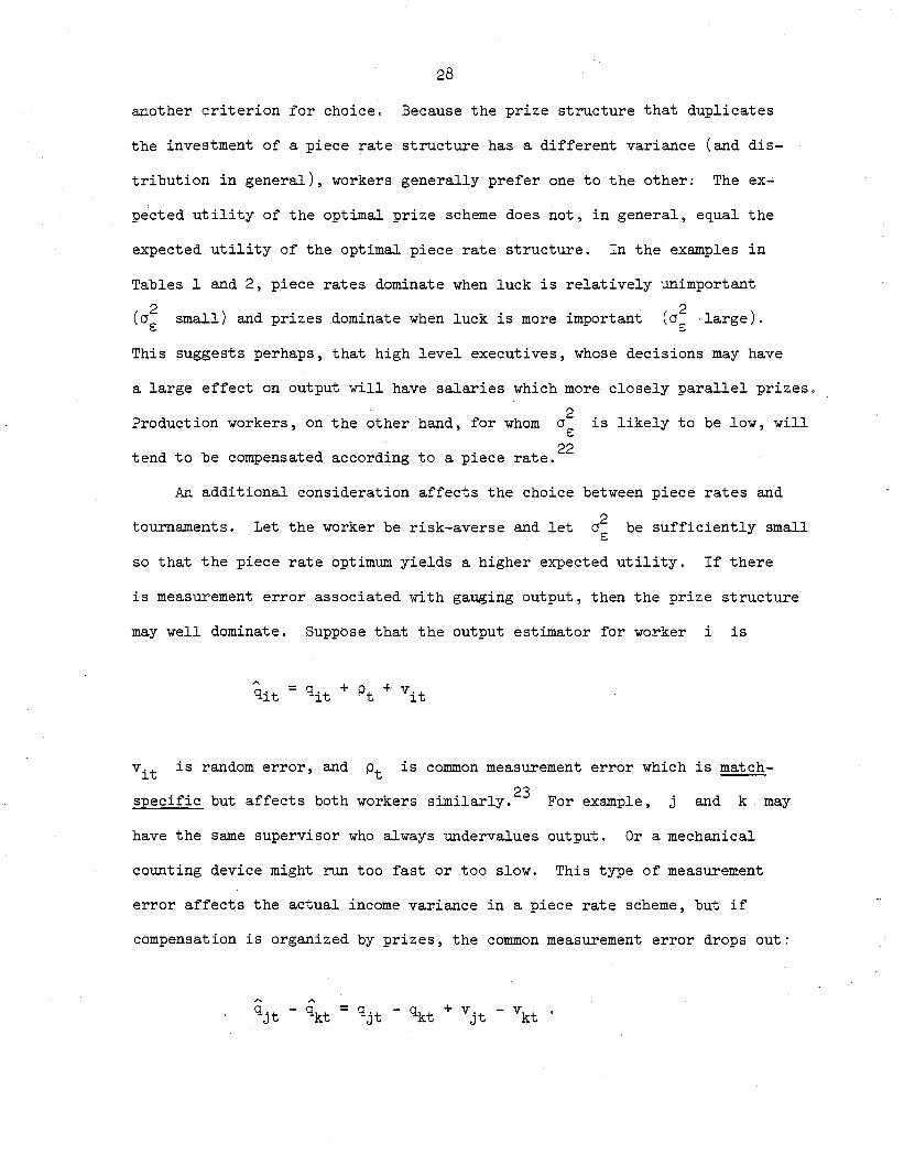
The same was done for a utility function of the quadratic form,

U = _y2 + 1000y. Table 2 contains those results:

Table 2

Quadratic Utility Function

2)l* E(U) - E(U*)(J )l

-f..

.01 .999 .999 .0211 .999 .993 2.12

100 .909 .614 92150 .869 .514 61200 .833 .443 -46.2

Both tables tell the same story. When (J2. 11·~s sma p~ece ratese:

2dominate, but when (J goes above some level a prize yields the largeste:

expected utility.

With risk-neutrality we showed that there is always a unique prize

structure that duplicates the resource allocation of the optimal piece-

rate wage structure: There, each compensation scheme yields the same

expected utility, and choice between them is on the basis of different

monitoring and observation costs. In this section, risk-aversion supplies

28

another criterion for choice. Because the prize structure that duplicates

the investment of a piece rate structure has a different variance (and dis-

tribution in general), workers generally prefer one to the other: The ex-

pected utility of the optimal prize scheme does not, in general, equal the

expected utility of the optimal piece rate structure. In the examples in

Tables 1 and 2, piece rates dominate when luck is relatively unimportant

(o~ small) and prizes dominate when luck is more important (cr~ ,large).

This suggests perhaps, that high level executives, whose decisions may have

a large effect on output will have salaries which more closely parallel prizes.

Production workers, on the other hand, for whom

tend to be compensated according to a

02E:

. t 22p~ece ra e.

is likely to be low, will

An additional consideration affects the choice between piece rates and

tournaments. Let the worker be risk-averse and let cr2 be sufficiently smallE:

so that the piece rate optimum yields a higher expected utility. If there

is measurement error associated with gauging output, then the prize structure

may well dominate. Suppbse that the output estimator for worker i is

vit is random error, and Pt is common measurement error which is match­

specific but affects both workers similarly.23 For example, j and k may

have the same supervisor who always undervalues output. Or a mechanical

counting device might run too fast or too slow. This type of measurement

error affects the actual income variance in a piece rate scheme, but if

compensation is organized by prizes, the common measurement error drops out:

A A

qjt qkt = qjt - qkt + V jt - vkt .

29

The sign of is unaffected by Contest-specific measurement

error adds no noise to the tournament, but does contribute variance to

piece rate income. Therefore, if

structure may dominate even if

2cr p is sufficiently large, the prizet

is small.

-D. Skewed Earnings Distribution with Risk-Aversion

In the risk-neutral world, we obtained a positively skewed distribution

of income by ,introducing contests with eliminations. Skewed overall income

distributions fallout of the analysis with risk-aversion quite easily.

Suppose that there are two occupations, A and B, and that all

individuals are alike. Let jls output in A or B be given by

m m=ll.+e:.

J Jm =: A,B

Assume for simplicity that costs of investment are the same in both

let it be the case that as the result of the

2> cr B. Further,

E:

a piece rate

2is inherently riskier, i.e., cr AE:

risk differences,

Aoccupations, but that

Those in B end up with income that reflects the distribution of

scheme is optimal for B, whereas the prize scheme is optimal for A.

BE: • If

that is normally distributed, then their incomes are normally distributed

with mean

either WI

BI + r].l

2 2and variance r cr B. Those in A receive incomes ofE:

Since A is inherently riskier than B, the expected

utility associated with A is lower than that for B at any common V.

Therefore, relative supplies of workers must adjust to increase the value

of services in A until expected utilities are equal across occupations.

This implies that the mean income in A must exceed the mean in B to

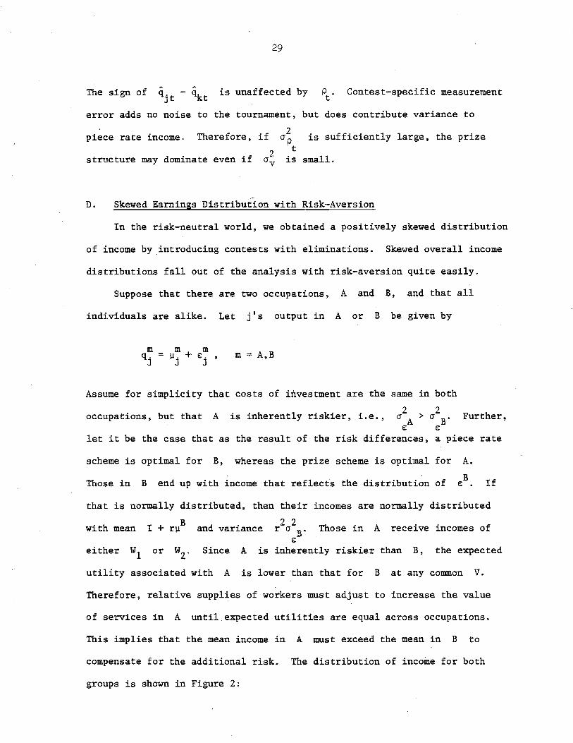
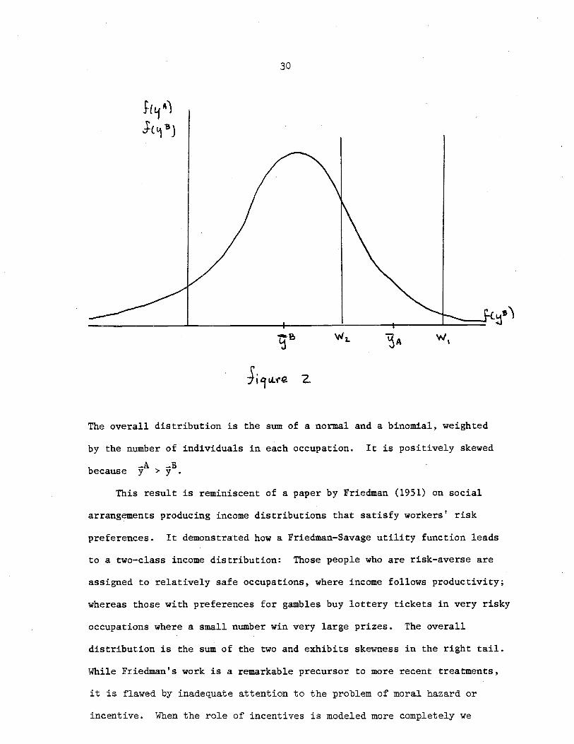
compensate for the additional risk. The distribution of income for both

groups is shown in Figure 2:

because

30

The overall distribution is the sum of a normal and a binomial, weighted

by the number of individuals in each occupation. It is positively skewed

_A _BY > Y .

This result is reminiscent of a paper by Friedman (1951) on social

arrangements producing income distributions that satisfy workers' risk

preferences. It demonstrated how a Friedman-Savage utility function leads

to a two-class income distribution: Those people who are risk-averse are

assigned to relatively safe occupations, where income follows productivity;

whereas those with preferences for gambles buy lottery tickets in very risky

occupations where a small number win very large prizes. The overall

distribution is the sum of the two and exhibits skewness in the right tail.

While Friedman's work is a remarkable precursor to more recent treatments,

it is flawed by inadequate attention to the problem of moral hazard or

incentive. When the role of incentives is modeled more completely we

31

obtain a similar result with only risk-aversion, since the optimum contract

is a tournament if the underlying distribution of outcomes has a large

variance.

V. HETEROGENEOUS CONTESTANTS

Workers are not sprinkled randomly across firms, but rather seem to be

sorted by ability levels. One explanation for this has to do with comple-

mentarities in production. But even in the absence of such complementarities,

sorting may be an integral part of optimal labor contract arrangements.

Therefore, this section analyzes tournament structures in the risk-neutral

case when investment costs differ among persons. Two types of persons are

assumed, a's and b's- , with marginal costs of the a's being smaller than

that of the b's: C~(~) <Cb(~) for all ~. The distribution of distur­

bances f(e) is assumed to be the same for both groups. Many of the fol-

lowing results continue to hold, with usually obvious modification of the

arguments, if the a's and b' s draw from different distributions. Part

A addresses the question of self-selection and part B discusses handicap

systems.

A. Adverse Selection

Suppose eac~ person knows which class he belongs to, but that this infor-

mation is not available to any player or firm. The principal result is that

the a's and b's do not self-sort into their own "leagues. " Rather every-

one prefers to play in the "major leagues;" all workers prefer to work in firms

with the best workers, even in the absence of production complementarities.

Furthermore, there is no price rationing mechanism that induces Pareto

optimal self-selection, and mixed play is inefficient because it cannot

32

sustain the efficient investment strategies. Therefore tournament

structures naturally require credentials and other nonprice signals to

differentiate people and assign them to the appropriate contest. Firms

will select their employees based upon some initial information and all

are not permitted to enter.

The proof of adverse selection is to assume "pure" contests a - a

and b - b and demonstrate that they are not viable. We know from

Section II that if a's play each other and b's play each other the

outcomes are efficient, since V = C~(~a) = Cb(~b). Suppose the market

is organized and sorted into separate a contests and b contests

satisfying Section II and contemplate which contest a given person, whether

an ~ or Q.., would choose to enter.

If a person has an arbitrary investment level ~. expected gross

revenue from entering league i = a,b is

(30) R = wi + (Wii 2 1 i = a,b

are winning andi i Wiwhere P is the probability of winning and WI' 2

losing prizes in league i contests. But if the market is perfectly

sorted then iP =G(~-··W':).

~

where is the existing players' (the

opponents') investment in that league, satisfying V = C ~ (~~) •~ ~

In

equilibrium W~ - W~ = V!g(O), from equation (12), in both leagues and

Wi = V~. - V/2g(O), from (11). Substitution into (30) yields2 ~

(31) i = a,b.

Several properties of 81) follow from Section II. First,

There is higher quality play in a - a which supports a larger total

purse and the spread is the same in both leagues. Second, since

G'(·) = g(.)

33

is symmetric with a maximum of g(O), G(~ _ ~~) = pi has1

an inflection point at Third, since G(O) = 1/2, direct evaluation

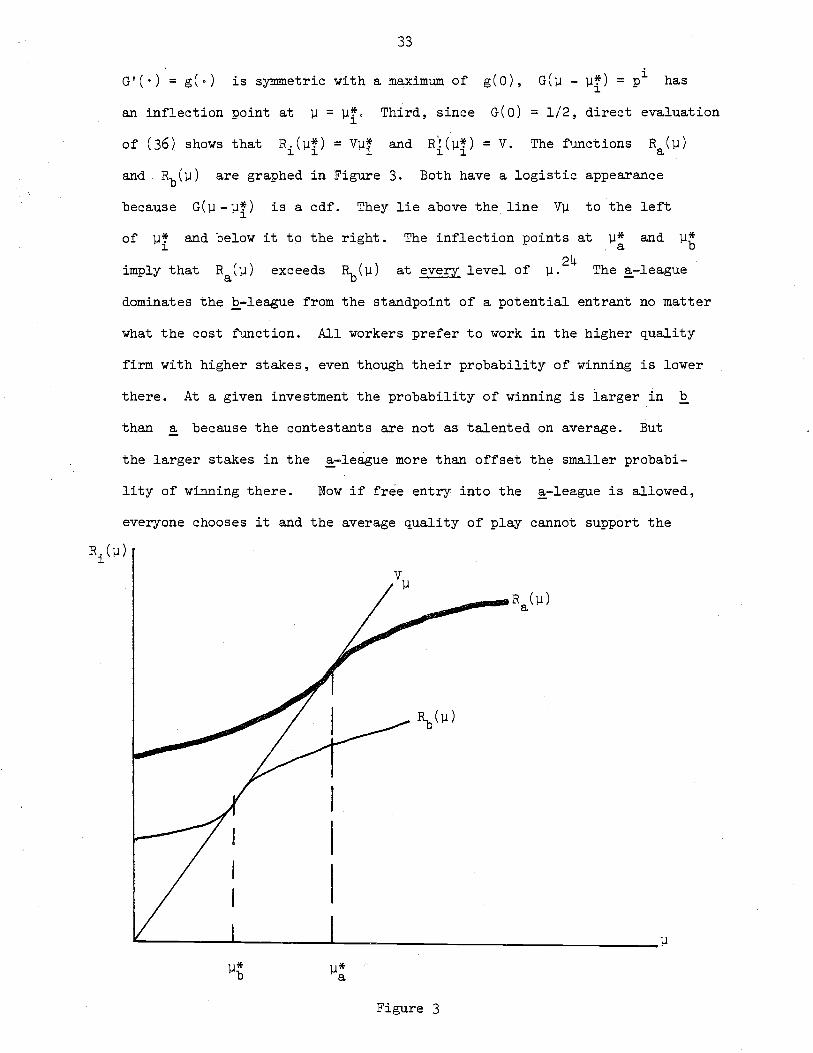
of (36) shows that The functions

and Rb(~) are graphed in Figure 3. Both have a logistic appearance

because is a cdf. They lie above the line to the left

imply that The §.-leagueat every level of

of ~~1

and below it to the right.

exceeds

The inflection points at

24~.

~*aand ~*b

dominates the E.-league from the standpoint of a potential entrant no matter

what the cost function. All workers prefer to work in the higher quality

firm with higher stakes, even though their probability of winning is lower

there. At a given investment the probability of winning is larger in b

than a because the contestants are not as talented on average. But

the larger stakes in the §.-league more than offset the smaller probabi-

lity of winning there. Now if free entry into the §.-league is allowed,

everyone chooses it and the average quality of play cannot support the

R. (~)1

~*b ~*a

Figure 3

separating equilibrium prize money (W~, W;) because total product is

contaminated by lower quality b's. The market structure collapses and

the assumed optimal separation is contradicted.

Since the demand for participation in b contests is effectively

zero, the obvious question is whether price rationing alone can achieve

market separation. The answer is no. The reason is that a single price

must be charged to all possible entrants, take it or leave it, because

the a's and b's cannot be recognized in advance. Yet a single price

does not give any differential incentives for either a's or b's to

enter the ~-league.

Again, initially assume separation and consider a ~-person who

invested ~ and contemplates jumping into the a-league. From (31) the

expected gain in income in a over b is

Similarly, the gain to an ~-person who, having committed investment ~:'

contemplates going from league b to league a is

But G(~* - ~*) = 1 - G(~* - ~*}b a a bso that The expected

gain from participation in league a to either an a or a b is the same

when both invest at their social optimum levels. Therefore any entrance

fee (over and above the gamble) has the same deterrent effect on entry for

either a's or b's. In particular, the price that absolutely deters b's

from entry also deters all of the a's. Of course, if a b anticipated

crashing an ~ contest he would do better by investing less than ~~.

35

That ~ould only make him a more eager participant, even a larger price

deterrent ~ould be necessary to keep him out and that surely turns a~ay

the a's.

If the price mechanism and pure self-interest do not separate markets

when cost information is asymmetric, does competitive equilibrium in mixed

firms yield the proper investment incentives? Generally the answer is no.

Suppose the proportion of ~'s in the population is .kno~ by everyone

to be a and the pairings are random so the chance of playing an ais a

and the chance of playing a b is (1 - a). Let the prizes in mixed play

P the probability of ~inning if matched against an aa

and Pb the ~inning probability if matched against a b. Expected utility

of a player of type i is

Wz + (aP~ + (1 - a )P~) (Wl

- Wz) - Ci

(lJi

)

Where pi is the probability of a win for a player of type i when hea

opposes an a, and similarly for

The first-order condition for "mixed investment" J.l. is~

.t oP; +cJ.l.

~

(l -cpiJb -

~)ClJi (WI - WZ) = C~ (J.l.)~ ~

A development similar to Section II reveals that in equilibrium 02) becomes

(ag(O) + (1 - a)g(~a - ~b)J(W1 - WZ

) =

( 33) for a's and

c' (~ )a a

for b I s.

Again, only spread matters for invest~ent decisions.

It is not entirely clear what competitive eqUilibrium looks like in

mixed contests when players' types are unknown, but perhaps a case can be

36

made that the net value of output is maximized subject to a zero profit

constraint and the Nash behavior implicit in (33). The chances of pairings

tively. Therefore expected product is

of a - a, a - b, and b - bare2

a , 2a(l - a) and

211 a2 + 2a(l ­

a

2(1 - a) respec-

22(1 - a) ~b = 2 [alla + (1 - a)~b] and the zero profit constraint is

The net value of output is

so the equilibrium maximizes (35) with respect to WI and W2 subject to

(33) and (34).

The first-order condition for the optimal spread ~W - WI

by differentiating (35):

W2 is found

( 36)

Though the solution v = C'(~ ) = C'(~)a a b . 0satisfies (36), examination of (33)

shows that it violates the equilibrium investment strategies except possibly

when a =~. In fact, the solution with mixed players is efficient only

when a =~. In that case, the optimal spread is given by ~W = V/(g(O) +

g(ll: - u~»/2. This is larger than the spread in pure contests because both

players invest less in mixed than pure play at any given spread. The spread

must be larger to induce greater investment. In all other cases, one type

of player overinvests and the other underinvests to satisfy (36), because

37

a~a/a6W and a~b/a6W are positive. Therefore a mixed league with no cost

revelation is almost always inefficient. Equation (33) implies that the a's

underinvest and the b's overinvest when a < ~ and the opposite is true

when a > ~.

We are led to the unalterable conclusion that a pure price system

cannot sustain an efficient competitive equilibrium in the presence of

population heterogeneity and private information. This does not say that

price competition cannot separate markets, but it does imply that if markets

are separated on the basis of price incentives alone then they must be

inefficient. It is easy to produce an example of such an equilibrum. The

a's want to differentiate themselves from the b's because they are

potentially more productive. Consider the following two contests. In one

the prize structure is set up as in Section II, equations (11) and (12).

In the other there is a much larger spread and a smaller losing prize.

Following the development of the first part of this section, assume that

only b's are attracted to the first type of contest and only a's to the

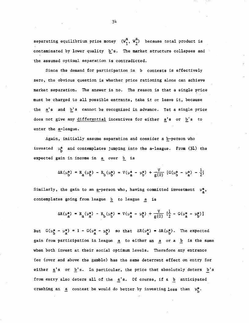
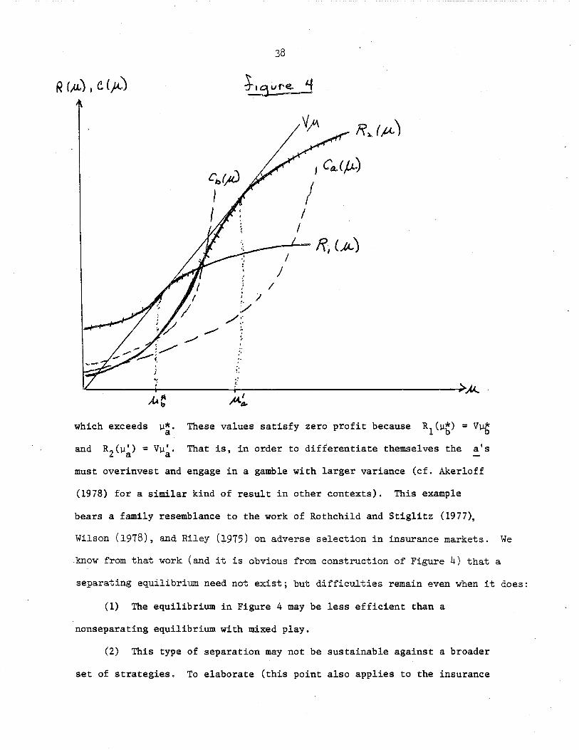
second. The situation is shown in Figure 4. The curve labeled R1(~) is

the expected payoff from entering the first type of contest at investment

~ and is identical to ~(~) in Figure 3. R2(~) is the expected payoff

to entering a contest with greater spread and smaller losing prize. It is

therefore steeper than R (~)a in Figure 3 and has a smaller intercept than

In distinction to Figure 3 where R (~)a everywhere dominated

for larger values. The overall return function is therefore the upper

envelope of these two curves. As illustrated, the b's find it optimal

to invest ~~, which is efficient for them; but the a's invest ,~a'

38

.,;

,

; I,.:/

/,'/",

,,,:.

II

I------.- If, (A.)

/J

/

which exceeds J.l*.a These values satisfy zero profit because R (J.l*) = Vj.I*1 b b

and That is, in order to differentiate themselves the a's

must overinvest and engage in a gamble with larger variance (cf. Aker10ff

(1978) for a similar kind of result in other contexts). This example

bears a family resemblance to the work of Rothchild and Stiglitz (1977),

Wilson (1978), and Riley (1975) on adverse selection in inSurance markets. We

.know from that work (and it is obvious from construction of Figure 4) that a

separating equilibrium need not exist; but difficulties remain even when it does:

(1) The equilibrium in Figure 4 may be less efficient than a

nonseparating equilibrium with mixed play.

(2) This type of separation may not be sustainable against a broader

set of strategies. To elaborate (this point also applies to the insurance

39

problem), suppose the leagues and prizes are set up as in Figure 4 with

players "signing" into a league prior to committing investment. The mere

act of signing into league 1 or 2 therefore reveals their type. But once

types are revealed all those labeled as a's can gain from trade: There

are post-signing incentives to set up yet another league that satisfies

conditions (11) and (12) for that yields higher rents for the a's than

league 2 and no game in league 2 is ever played. If that happens no b

signs up in league 1, knowing that signing in the "dummy" league 2 labels

him an a and ultimately entitles participation in what appears to be a

dominant game, as in Figure 3. This behavior, akin to a time inconsistency,

unravels the two-league structure and separation is not achieved.

The practical resolution of these difficulties, which has its obvious

counterpart in the structure of real-life tournaments, is the use of

nonprice rationing and certification to sort people into the appropriate

games, based on past performances. Similarly, firms use nonprice factors

in allocating jobs among applicants. Presumably the market solves a

complicated experimental design problem, perhaps with a hierarchical

structure, that elicits this information in an efficient manner. The

issues are similar to those sketched in Section III.B.

Upon reflection, it is not terribly paradoxical that price information

alone does not allocate resources efficiently in these circumstances and

that nonprice rationing can be more effective. After all, only a fool or

a person with tastes for random dissipation of his wealth would examine

only the price of a transaction when there is a nontrivial probability of

misrepresentation of the other terms. That nonprice factors are

ubiquitous in labor markets is recognized in the theory of equalizing

differences. For practical examples of nonprice rationing one need go no

40

further than the problem of allocating academic economists to departments.

Yet there appears to be a special problem with tournament structures that

should be pointed out. Strictly speaking, in the formal model above there

is no social value of sorting inherent in the technology, since total

output is the sum of independent outputs of all the workers. The tournament

introduces a socially contrived dependence through strategic factors

involved with attempting to improve one's chance of winning, for which

relative output is crucial. The independence of production implies that

sorting is no problem in the piece rate solution when workers are risk­

neutral: It makes no difference who works with whom because rewards are

based on independent individual performance?5 Of course, there would be

productive value of sorting if the objective function were not summable,

e.g., V(qj,qk) or the order statistic example in Section III.C instead

of V· (qj + qk). Nevertheless, the above differences may suggest that

stratification and sorting present greater difficulties for tournaments

than for individual performance-geared incentive schemes. Still,

tournaments may be the socially efficient arrangement if rank is easier

to observe than is individual performance.

B.Handicap Systems

This section moves to the opposite extreme of the previous discussion

and assumes that the identities of each type of player are known to everyone.

Gambles involving N players of known talent are said to be fair if each

player has win probability of liN. When the quality of play is drawn out

of fixed distributions that differ among players, fairness is achieved by

handicaps that equalize the upper liN quantiles of the various

41

distributions; e.g., with N = 2 the weaker player is given "points" to

equalize the medians. It is surprising that this criterion of fairness

fails to hold true in competitive markets where prizes affect probability

distributions and the gambles are productive: The market clearing handicap

implies less than full equalization so that the better player always has a

competitive edge.

Consider again two types a and b now known to everyone. Prize

structures in a - a and b - b tournaments satisfying (11) and (12) are

efficient, but those conditions are not optimal in mixed a - b play.

Denote the socially optimal levels of investment by lJ* and lJ~ , theira

difference by LllJ, and the prizes in a mixed league by WI and W2

, Let

h be the handicap awarded to b with LllJ ~ h ~ O. Then the Nash solution

in the a - b tournament satisfies

C' (lJ )a a

(37)

(The second condition in (37) follows from symmetry of g(~).) Since

independence of outcomes implies no social preference for alternative

structures when revenues are additive, the efficient investment criterion

is v = C'(lJ*) = C' (u:k)a a b . b 'independent of pairings, Therefore from (37)

the optimum spread in a mixed match must be

(38) LlW = V/g(LllJ - h)

to induce proper investments by both contestants. The spread is larger

in mixed than pure contests unless a gives b the full handicap

42

h = ~~ - ~~. Otherwise, the appropriate spread is a decreasing function of

h. - - -and Wz must also satisfy the zero profit constraint WI + Wz =

v . (~~ + ~~) independent of h since the spread is always adjusted to

induce investments ~~ and ~~.

The gain to an a from playing a b with handicap h rather than

another a with no handicap is the difference in expected prizes since

costs are the same in all matches C (~*):a a

Y (h)a

where P = G(A~ - h) is the probability that a wins the mixed match.

The corresponding expression for b is

The zero profit constraints in a - a, a - band b - b imply that

ya(h) + yb(h) = 0 for all admissible h; so the gain of playing mixed

matches to a is completely offset by the loss to b and vice versa.

If Ca(~) is not greatly different from Cb(~) then

A~ = ~: - ~~ is small and P ~ t + g(A~ - h). This approximation and

the zero profit constraint reduce (39) to

(41) Y (h) ~ -VA~ r:i _ g(O) (l _ J!.)la l: g(A~ - h) A~J

The expression for yb(h) is the same except for the absence of the minus

sign in front of VA~. y~(h) = -yb(h) < 0 so the gain to a decreases in

h and the gain to l increases in h. Moreover,

Y (0) = Vt.].l [g(O) - 1] > 0 and Y (t.].l) = -Vt.].l/2. Therefore there existsa g(t.].l) 2 a

a unique h* satisfying Ya(h*) = yb(h*) = 0 and 0 < h* < t.].l.

If the actual handicap is less than h* , a's prefer to play in mixed

contests rather than with their own type while b's prefer to play with

~'s only. The opposite is true if h > h*. Since the gain to the one is

the loss to the other, side payments and guarantees could induce b's to

play against a's in the first case and a's to play against b's in the

second. However, side payments are unnecessary when h = h*, for then no

one cares who they are matched against. Therefore h* is the competitive

market clearing handicap and the condition 0 < h* < t.].l implies that it is

less than full. The a's are given a compe~itive edge in equilibrium,

- 1 1p ~ 2 + g(t.].l - h*) > 2 because they contribute~ to total output in

mixed matches than the b's do. This same result holds if € has aa

different variance than €b' but may be sensitive to the assumption of

statistical independence and output additivity.

VI. SUMMARY AND CONCLUSIONS

This paper proposes an alternative to compensation in proportion to

marginal product. Under certain conditions, the new scheme yields ~~ allo-

cation of resources identical to that generated by the efficient piece rate.

By compensating workers on the basis of their relative position in the firm,

one can produce the same incentive structure for risk neutral workers that

the optimal piece rate produces. It might be less costly, however, to

observe relative position than to measure the level of each worker's output

directly. This would result in paying salaries which resemble "prizes";

wages which for some workers greatly exceed their presumed marginal products.

44

When risk aversion is introduced~the prize salary structure no longer

duplicates the allocation of resources induced by the optimal piece rate.

For activities which have a high degree of inherent riskiness~ contests will

tend to dominate. For sufficiently small levels of inherent riskiness~ the

competitive piece rate tends to dominate. Given risk aversion~ a positively

skewed overall distribution of income is the natural outcome of the mixing

of the distribution of income for those paid prizes with that for those paid

piece rates.

Finally, we allow workers to be heterogeneous. This complication adds

an important result: Competitive contests will not, in general, sort workers

in a way which yields an efficient allocation of resources. In particular,

low quality workers will attempt to contaminate the firm comprised of high

quality workers, even if there are no complementarities in production. This

contamination results in a general breakdown of the efficient solution if

low quality workers are not prevented from entering. This is, therefore, one

rationalization for the use by high quality firms of initial credentials when

allocating jobs to applicants.

45

FOOTNOTES

1. This statement needs qualification. For example, annual bonuses may

depend on group measures such as total profits of the firm, but not on

rank order of workers within each labor category.

2. Virtually all the results of this paper hold true if the error structure

is multiplicative rather than additive, but the exposition is slightly

less convenient in the case.

3. Throughout the analysis, we assume that the worker has control only over

~. A more general specification would allow him to affect the variance

of E. Although this will not alter the solution in the risk neutral

case, risk averse workers might sacrifice ~ for lower variance of E.

This problem, of inducing the worker to avoid cautious strategies, is

one which we do not analyze here.

4. A nonlinear piece rate schedule r(q) provides the correct marginal

incentives so long as r'(q) = V at equilibrium. It is clear that a

one-parameter linear piece rate is the competitive solution in this

case, since nonlinearities or two-part tariffs can only transfer

inframarginal rents to employers, thus violating the zero profit

condition. A one-parameter piece rate is definitely nonoptimal in

the presence of risk aversion. See below.

5. Since a~P = g(~j -~) and g(.) is a pdf, a2P/a~~ = g'(~j - ~k)j

may be positive and fulfillment of second-order conditions in (5) may

imply sharp breaks~in the reaction function. See the appendix for

elaboration.

46

6. With normal errors (12) and (8) imply

The ratio of the spread to the mean prize is proportional to the

coefficient of variation of output. This formula also applies toN

an N-player game with WN replacing W2 in the numerator and rWi/N

in the denominator.

7. Of course, in a full analysis any change in costs of all participants

would change industry supply and therefore alter V, but those

qualifications are straightforward.

8. Lazear (1979, 1979a) uses this notion in a deterministic but dYnamic

setting. By paying an individual more than his marginal product later

in life, and less than marginal product earlier in life, one induces

optimal effort and investment behavior throughout the worker's lifetime.

9. Of course, the risk is diversifiable across workers and therefore by

firms. One might also think that risks could therefore be pooled

among groups of workers through, say, sharing agreements, but that

is false because of moral hazard. A worker would never agree to share

prizes since doing so (completely) results in ~ = 0 so that E(qj + qk) = O.

As the result, firms offering tournaments' or piece-rates in the pure sense

yield higher expected utility than the sharing arrangement.

10. There is some discussion of contests in the statistics literature for

the method of paired comparisons. Samples from different populations

are compared pairwise and the object is to choose the one with the

largest mean. If all pairs are compared, the experimental design is

similar to a round-robin tournament. An alternative design is a

47

knockout tournament with single or double elimination, which does not

generate as much information as the round-robin but which requires

fewer samples and is cheaper. These problems are discussed by David (1963)

and Gibbons, Olkin and Sobel (1977), but are not helpful here because

they assume fixed populations, whereas the essence of our problem is

to choose an experimental design and payoff mechanism that induces

players to choose the correct distributions to draw from. A complete

treatment would add the additional complexity of allowing investment

strategies to change as new information becomes available.

11. With the current technology and risk neutral workers, there is no

advantage to being able to distinguish the best from second-best,

etc. The motivation for this analysis comes from considering other

payoff structures where level is important in nonadditive ways. A

multiplicative technology, where revenue equals Vf(qjqk), for example,

implies that sorting of workers is important. Similarly, a payoff

which depends on the level of the highest output individual may also

require sorting. This latter case is discussed below in another context.

12. Strictly speaking, the production variables in the two-period problem

should be rescaled to make the outcomes identical with Section II, but

that is a detail.

13. See Lazear (1979) for additional details.

14. Economies of joint consumption, in some activities such as performance,

may imply very large rewards to a small number of people. To a

potential entrant the game might look like a lottery based on rank

order and it may appear as if consumers value rank perse. See Rosen

(1979) for elaborat ion.

48

15. We are indebted to George Stigler for this reference. There is a

well-known paper by Mosteller (1951) on how many games must be played

before one is fairly certain that the best team emerges victorious,

as well as the literature on paired comparisons referred to above,

but these are not directly relevant.

16. The following is similar to a problem analyzed by Stiglitz (1915). A

linear piece rate structure is a simplification. A more general

structure would allow for nonlinear piece rates (see Mirrlees, 1916).

A still more general model allows for the compensation scheme to be a

random variable. Prescott and Townsend (1919) consider this in the

11.

context of a selection problem.

Furthermore, r::: V/(l + sC"cr2 )e:

r = V and I = ° in the case of risk ·aversion, s = 0, as asserted

in Section II. All these approximations use first-order expansions

for terms in U'(.) and second-order expansions for terms in U(·).

The same is true of the approximations below for the tournament.

18. With N players and N prizes (WI the first place prize, W2 secondN

place, etc.) equation (25) becomes C,(~) =k[U(l) - U(N)]/EU'(T), where

k is a constant. As in Section III.A, the numerator contains terms

only in first and last place prizes. But now the denominator contains

terms in all the other prizes as well, removing the source of indeter-

minacy of the entire prize structure that occurred in the risk-neutral

case.

19· Furthermore, C,(~*)::: g(O)(Wl - W2), so the spread is still crucial

for investment incentives, as in the risk-neutral case.

49

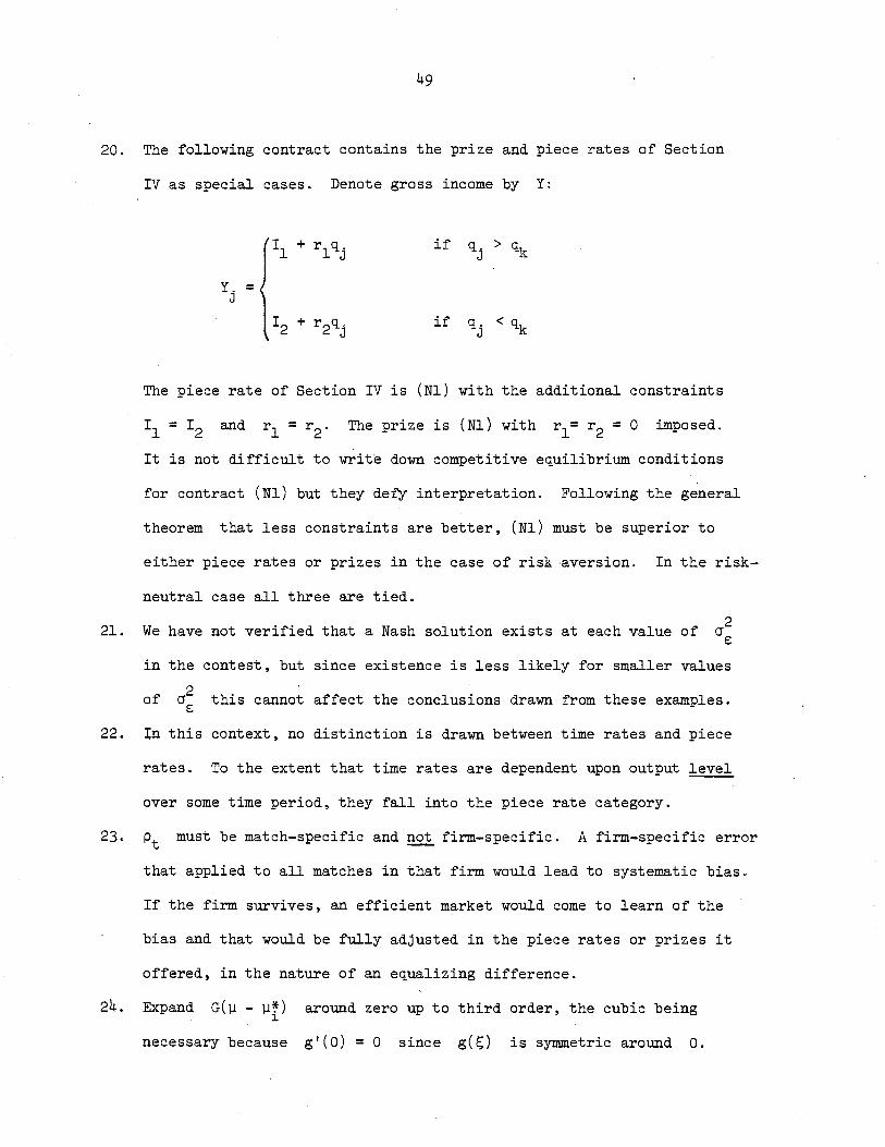
20. The following contract contains the prize and piece rates of Section

IV as special cases. Denote gross income by Y:

11 + r l qj if qj > qk

Y. =J

12 + r 2qj

if qj < qk

The piece rate of Section IV is (Nl) with the additional constraints

and The prize is (Nl) with imposed.

It is not difficult to write down competitive equilibrium conditions

for contract (Nl) but they defy interpretation. Following the general

theorem that less constraints are better, (Nl) must be superior to

either piece rates or prizes in the case of risk ·aversion. In the risk-

neutral case all three are tied.

21. We have not verified that a Nash solution exists at each value of cr~

in the contest, but since existence is less likely for smaller values

of cr2 this cannot affect the conclusions drawn from these examples.€:

22. In this context, no distinction is drawn between time rates and piece

rates. To the extent that time rates are dependent upon output level

over some time period, they fall into the piece rate category.

23. Pt must be match-specific and not firm-specific. A firm-specific error

that applied to all matches in that firm would lead to systematic bias.

If the firm survives, an efficient market would come to learn of the

bias and that would be fully adjusted in the piece rates or prizes it

offered, in the nature of an equalizing difference.

24. Expand G(~ - ~~)~

around zero up to third order, the cubic being

necessary becaus.e g'(O) = 0 since g(F;) is synnnetric around O.

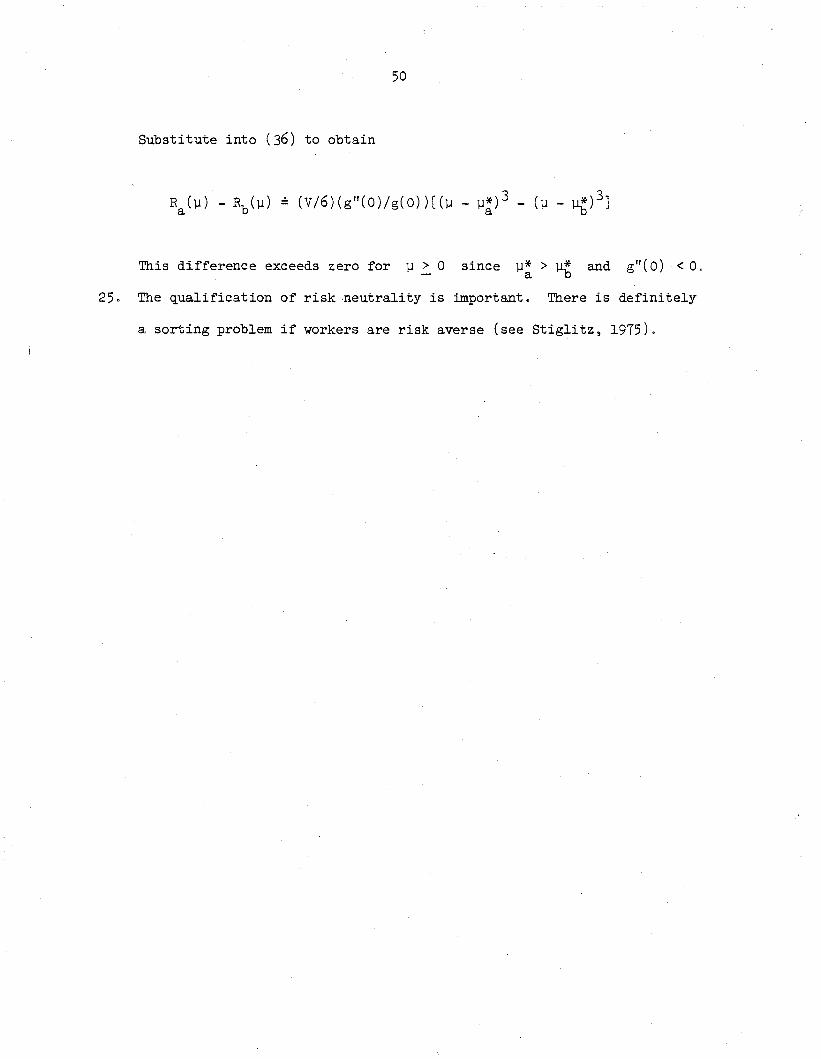
50

Substitute into (36) to obtain

This difference exceeds zero for ]..1 > 0 since ]..1* > ]..1b* and g"( 0) < o.- a

25. The qualification of risk neutrality is important. There is definitely

a sorting problem if workers are risk averse (see Stiglitz, 1975).

51

REFERENCES

Alehian , A.A. and H. Demsetz. "Production, Information Costs and EconomicOrganization," American Economic Review. LXII, No.5 (pp. 777-795)December, 1972.

Becker, G. and G. Stigler. "Law Ecforcement, Malfeasance and Compensationof Enforcers," Journal of Legal Studies. (pp. 1-18) 1974.

Cheung, Steven. The Theory of Share Tenacy: With Special Application toAsian Agriculture and the First Phase of Taiwan Land Reform. Chicago:University of Chicago, 1969.

David, H.A. The Method of Paired Comparisons. London: Charles Griffin,1973.

Friedman, M. "Choice, Chance and the Personal Distribution of Inc9me,"Journal of Political Economy. Vol. LXI, No.4 (pp. 277-90) August,1953.

Galton, Francis. "The Most Suitable Proportion Between the Values of Firstand Second Prozes," Biometrika. Vol. 1 (pp. 385-390) London: Cam­bridge University Press, 1901-1902.

Gibbons, J.D., I. Olkin and M. Sobel. Selecting and Ordering Populations:A New Statistical Methodology. John Wiley and Sous, New York: 1977.

Harris, M. and A. Reviv. "Some Results on Inceptive Contract with Applica­tion to Education and Employment, Health Insurance and Law Enforcement,"American Economic Review. Vol. 68, No.1 (pp. 20-30) 1978.

Lazear, Edward. "Why Is There Mandatory Retirement," Journal of PoliticalEconomy. December, 1979.

"Agency, Earnings Profiles, Productivity and Layoffs,"unpublished draft. Chicago: University of Chicago, April, 1979, (1979a).

Mirrlees, J.A. "The Optimal Structure of Incentives and Authority Withinan Organization," Bell Journal of Economics. Vol. 7, No.1 Spring, 1976.

Mosteller, F. "Remarks on the Method of Paired Comparisons; the Least SquaresSolution Assuming Equal Standard Deviations and Equal Correlations,"Psychometrika. Vol. XVI, pp. 3-11 Colorado: Psychometrika Society,January-December, 1951.

Prescott, E. and R. Townsend. "On the Theory of Value with Private Infor­mation," unpublished. Carnagie-Mellon University, 1979.

Riley, J. "Competitive Signalling," Journal of Economic Theory. Vol. 10(pp. 174-186) 1975.

Rosen, Sherwin. "Economics of Superstars," unpublished. University ofChicago, 1979.

52

Ross, Steve. "An Economic Theory of Agency," American Economic Review.Vol. 63, No.2 (Pl'. 134-139) May, 1973.

Rothchild, M. and J. Stiglitz. "Economics in Competitive Insurance Markets:The Economics of Imperfect Information," Quarterly Journal of Economics.Vol. XC, No. 4(361) (Pl'. 629-649) November, 1976.

Stiglitz, J.E. "Incentives, Risk and Information: Notes Towards a Theoryof Hierarchy," Bell Journal of Economics. Vol. 6, No.2 (Pl" 552-579)Autumn, 1975.

Wilson, Charles A. "A Model of Insurance Markets with Incomplete Information,"Journal of Economic Theory. Vol. 16 (2) (Pl'. 167-207) December, 1977.

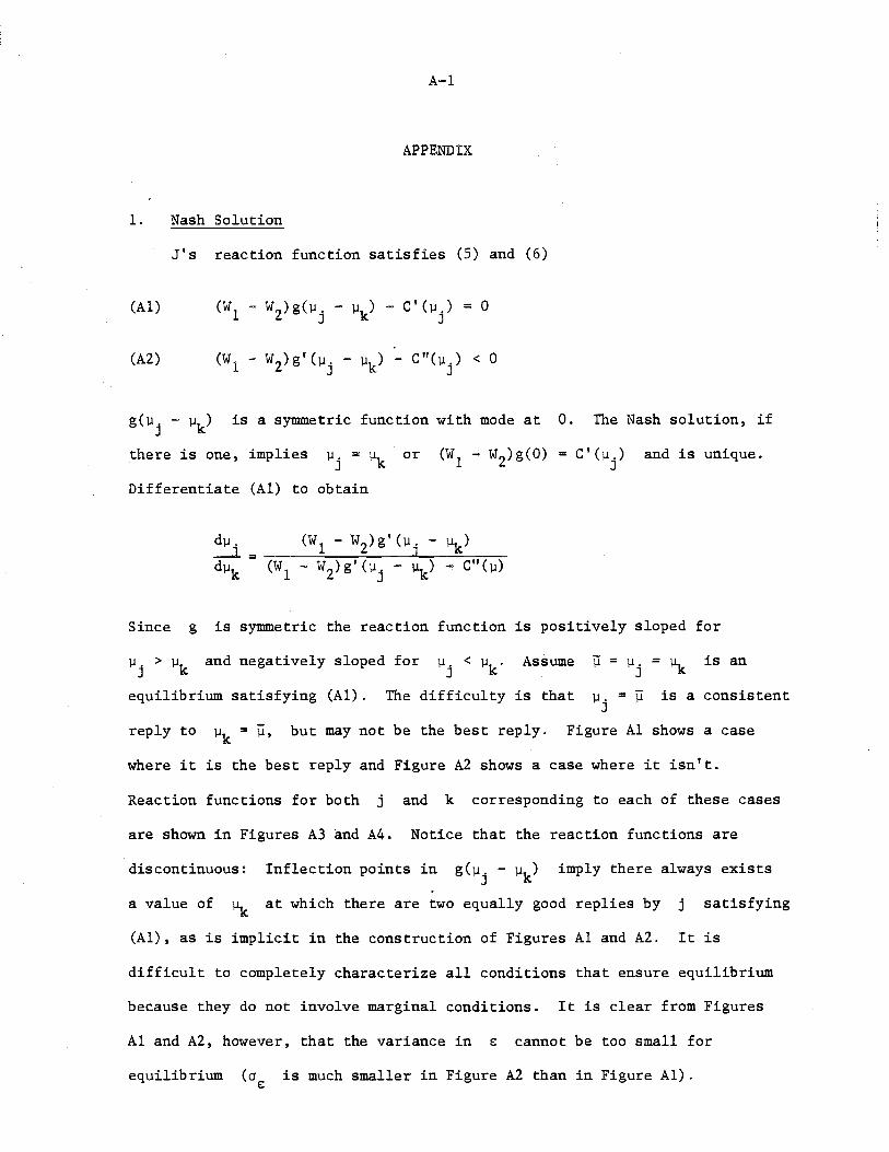
A-I

APPENDIX

1. Nash Solution

(AI)

(A2)

J's reaction function satisfies (5) and (6)

(w W)g'( ) - C"(".) < 01 - 2 llj - llk "J

g(llj - llk) is a symmetric function with mode at O. The Nash solution, if

there is one, implies llj :0 llk or C'(ll.)J

and is unique.

Differentiate (AI) to obtain

Since g is symmetric the reaction function is positively sloped for

llj > llk and negatively sloped for llj < llk' Assume jj = ll. = llk is anJ

equilibrium satisfying (AI) . The difficulty is that llj = jj is a consistent

reply to II = ii, but may not be the best reply. Figure Al shows a casek

where it is the best reply and Figure A2 shows a case where it isn't.

Reaction functions for both j and k corresponding to each of these cases

are shown in Figures A3 and A4. Notice that the reaction functions are

discontinuous: Inflection points in g(llj - llk) imply there always exists

a value of llk at which there are two equally good replies by j satisfying

(AI), as is implicit in the construction of Figures Al and A2. It is

difficult to completely characterize all conditions that ensure equilibrium

because they do not involve marginal conditions. It is clear from Figures

Al and A2, however, that the variance in s cannot be too small for

equilibrium (as is much smaller in Figure A2 than in Figure AI).

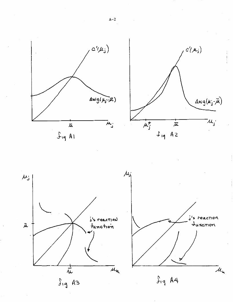
A-2

~

J '1 A2

"u,.J

i I'j, 't'~4..t..,."rJ

+a..7\C+,cm

?~

.) I, I"e4.cT,Ot\

-'----- .J.U.llc...T'OY\

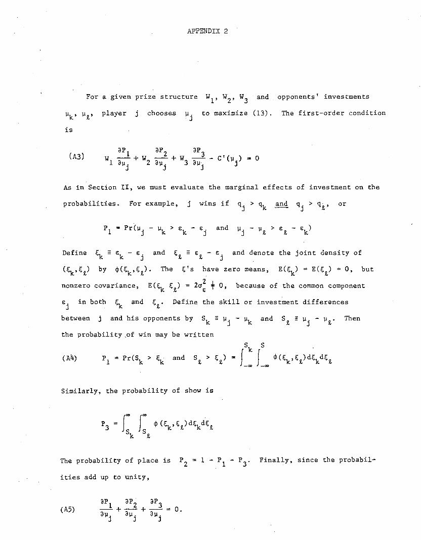
APPENDIX 2

For a given prize structure WI' W2

, W3

and opponents' investments

is

chooses ll.]

to maximize (13). The first-order condition

ap ap ap(1\3) W _1 + W _2 + W _3 - C' (ll .) = 0

1 all. 2 all 0 3 all]o ]] ]

As in Section II, we must evaluate the marginal effects of investment on the

probabilities. For example, j wins if or

and

Define ~k = £k - £j and ~t = £t - £j and denote the joint density of

(~k'~t) by ¢(~k'~t)· The ~'s have zero means, E(~k) = E(~t) = 0, but

nonzero covariance, E(~k ~t) = 20; +0, because of the common component

£j in both ~k and ~t. Define the skill or investment differences

between j and his opponents by and Then

the probability ,of win may be written

Similarly, the probability of show is

The probability of place is P2 = 1 - PI - P3

. Finally, since the probabil~

ities add up to unity,

(A5)

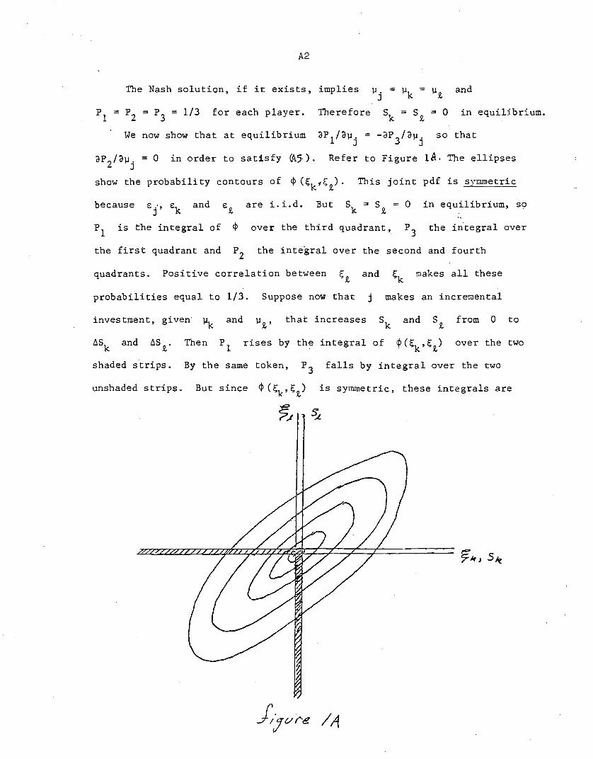
A2

The Nash solution, if it exists, implies ~j = ~k = ~t and

P = P = P = 1/3 for each player. Therefore Sk = Sn = 0 in equilibrium.1 Z 3 "-

We now show that at equilibrium aPl/a~j = -aP3/a~j so that

ap Z/dllj = 0 in order to satisfy (4.5·). Refer to Figure Itt, The ellipses

show the probability contours of </>·(i;;kfi;;t). This joint pdf is symmetric

because E: .', E:k

and E: tare Ll.d. But Sk = St = 0 in equilibrium, so

J

PI is the integral of </> over the third quadrant, P3 the integral over

the first quadrant and Pz the inte-gral over the second and fourth

quadrants. Positive correlation between ~t and ~k makes all these

probabilities equal to 1/3. Suppose now that j makes an incremental

investment, given ~k and ~t' that increases Sk and St from 0 to

65k and 65t

. Then PI rises by the integral of </>(~k'~t) over the two

shaded strips. By the same token, P3

falls by integral over the two

unshaded strips. But since <I>(~k'~t) is symmetric, these integrals are

~ ~

A3

equal and opposite in sign and P2 is unchanged. Therefore aP2/a~j = 0

and the optimum condition (A3) reduces to

~)

Finally) elementary manipulations.of (A4) imply

which is just the marginal density of ~k evaluated at ~k = O.

Substituting this into (A6) gives

i = j,k)i

which is virtually identical to equation (7) of Section II.

Note two things: First) Wz does not appear in ~6). This is the

source of the indeterminacy. Any Wz suffices so long as

1V~ = 3 [WI + Wz + W

3] ~ C(~j). Second) again only the win-show spread is

important in the determination of investment. The intuition is clear. A

risk-neutral player views games as equal so long as they have the same

expected value. Thus) increasing Wz and reducing WI and W3

but

leaving (WI - W3

) unchanged has no effect on the expected value of the

game. And because it leaves the spread between WI and W3

unchanged)

it does not change the value of ~. It is) therefore) like a lump-sum tax

coupled with offsetting lump-sum subsidies) and does not affect behavior.

As mentioned in the text, the indeterminacy vanishes when risk-aversion

is introduced.