NBER WORKING PAPER SERIES

MONOPOLISTIC COMPETITION, AGGREGATEDEMAND EXTERNALITIES AND

REAL EFFECTS OF NOMINAL MONEY

Olivier 3. Blanchard

Nobuhiro Kiyotaki

Working Paper No. 1770

NATIONAL BUREAU OF ECONOMIC RESEARCH1050 Massachusetts Avenue

Cambridge, MA 02138December 1985

We thank Andy Abel, Rudi Dornbusch, Bob Hall, Jeff Sachs, LarrySummers and Marty Weitzman for useful discussions. The researchreported here is part of the NBER's research program in EconomicFluctuations. Any opinions expressed are those of the authors andnot those of the National Bureau of Economic Research.

NBER Working Paper #1770Decenber 1985

t'tnoçolistic Canpetition, Aggregate DenendEcternaljH_es and Peal Effects of Nominal bney

Olivier CI. BlanchardDeparbient of EconomicsM.I.T.Cartridge, MA 32139

Nthuhiro KiyotakiDepartnent of EconomicsUniversity of Wisconsin1180 Cbservatory DriveMadison, WI 53706

A long etanding issue in macroeconomics is that of the relation

competition to fluctuations in output. In this paper we e,amine

monopolistic competition and the role of aggregate demand in th

output. We first show that monopolistically competitive economi

aggregate demand externality. We then show that, because of thi

menu costs, that is small costs of changing prices may lead to

aggregate demand on output and on welfare.

of imperfect

the relation between

e determination of

es exhibit an

s externality, small

large effects of

A long standing issue in macroeconomic, Ii that of the relation of Imperfect

competition to fluctuation! in output. In this paper we examine the relation between

monopolistic competition and the role of aggregate demand in the determination of

output. We first show that monopolistically competitive economies exhibit an

aggregate demand externality. We then show that1 because of this externality, small

menu costs, that is small cost of changing prices may lead to large effects of

aggregate demand on output and on welfare.

The paper is organized as follows. Section I builds a simple general equilibrium

model, with monopolistic competition in both labor and goods markets, and with

nominal money it then characterizes the equilibrium. Section II characterizes the

inefficiency associated with monopolistic competition and shows the inefficiency to

be due to an aggregate demand externality. Bection III studies the effect, of change!

in nominal money, when money is the numeraire, and when there are small, second

order, costs of changing prices. It shows that changes in nominal money may have

first order effects on output and welfare, and shows the close relation between this

result and the results obtained in Section II.

Section I. A model of monopolistic competition

We want to construct a model in which each price setter is large in its own

market but small with respect to the economy. The most convenient assumption is that

of monopolistic competition. The simplest model of monopolistic competition, for our

2

purposes, would be one of households using labor to produce differentiated goods.

However, because we want to focus later on both wage and price decisions, and want

the model to be easily comparable to the standard macroeconomic model, we construct a

model with both households and firms, and with separate labor and goods markets. Both

labor and goods markets are monopolistically competitive. Each firm sells a product

which is an imperfect substitute for other products each household sells a type of

labor which is an imperfect substitute for other types. The assumption of

monopolistic competition in both sets of markets is made for symmetry and

transparence rather than for realism. Although we choose to interpret suppliers of

labor as individual households, an alternative interpretation is to think of them as

unions or syndicates (as in Hart C 1982)).

The second choice follows from the need to avoid Says law, or the result that

the supply of goods produced by the monopolistically competitive firms automatically

generates its own demand. To avoid this, we must allow agents to have the choice

between consumption of these goods and something else. In the standard macroeconomic

model, the choice is between consumption and savings. In other models of monopolistic

competition, the choice is between produced goods and a non produced good (Hart, 1982

for example), or between produced goods and leisure (Startz 1985). Here, we shall

assume that the choice ts between buying goods and holding money. This is most simply

and most crudely achieved by having real money balances in the utility function of

agents. Thus, money plays the role of the non produced good and provides services'2.

A Glower constraint would lead to similar results. Developing an

explicitly intertemporal model just to justify why money is positively valueddoes not seem worth the additional complexity here.

There are however differences between money and a non produced good,which arise from the fact that real, not nominal money balances enter utilitywe shall point out differences as we ao along.

3

Money is also the numeraire, so that firms and workers quote prices and wages in

terms of •cney p this will play essentially no role in this and the newt section, but

will become important in Section ill

The third choice is to sake assumptions aboututility and technology which lead

to demand antpricing relations which are as close to traditional ones as possible,

so as to allow an easy co.parison with standard macroeconomic models. This however

sometimes requires strong restrictions on utility and technology, which we shall

indicate as we go along

The model3

The economy is composed of m firms, each producing a specific good which is an

imperfect substitute for the other goods, and n consumer— workers, households for

short, each of them owning a type of labor which is an imperfect substitute 4cr the

other types. As a result, each firm has some monopoly power when it sets its price,

and each worker has some monopoly power when he sets his wage4. We now describe the

problem faced by each firm and each household.

Firms are indexed by i, i 1,... ,m. Each firm i has the following technology

n -1 I

CI) V1 = ( E N.3 •i ) jrjj=l

The model can be viewed as an extension of the Dixit—Stiglitz (1977)model of monopolistic competition to macroeconomics.

Since in equilibrium each labor supplier sells some of his labor to allfirms, it is again more appropriate to think of labor suppliers as craftunions rather than individual workers. However since we want to analyze laborsupply and consumption decisions simultaneously, we shall continue to refer tolabor suppliers as "consumer—workers' or households.

4

Vs denotes the output of firm I. Ni., denotes the quantity of labor of type i

used in the production of output i. There are n different types of labor, indexed i,

1,... ,n. The production function is a CES production function, with all inputs

entering symmetrically3.

The two parameters characterising the technology are s and o. The parameter u Is

equal to the elasticity of substitution of inputs in production ; it will also be the

elasticity of demand 4cr each type of labor with respect to the relative wage. The

parameter is equal to the inverse of the degree of returns to scale —1 will be

the elasticity of marginal cost with respect to output —elasticity of marginal cost

for short in what follows—. To guarantee the existence of an equilibrium, we limit

ourselves to the case where is strictly greater than unity and where m is equal to

or greater than unity.

Each period, the firm maxinises profits. Nominal profits for firm i are given by

n

(2) V = PV — E W N±

P1 denotes the nominal output price of firm i. It, denotes the nominal wage

associated with labor type j. The firm maximises (2) subject to the production

function (1) • It takes as given nominal wages and the prices of the other outputs. It

also faces a downward sloping demand schedule for its product, which will be derived

below as a result of utility maximisation by households. We assume that the number of

firms is large enough that taking other prices as given is equivalent to taking the

price level as given.

We take the number of firms as given. The issue of whether there arefixed costs of production tan therefore be left aside.

5

Households are indewed by j, j al,... ,n. Houi,hold j supplies labor of type j.

It derives utility from leisure, consumption and real money balances. Its utility

function is given by i

1—1 p(3) Ui CC) (Mi/P) —

6—1 9where C E C116) 6-i

i :1m 1—6 1

and P EP. )1—9m i1

The first term, Cj, is a consumption index —basket— which gives the effect of

the consumption of goods on utility, C±. denotes the consumption of good i by

household j. C., is a CES function of the C s. All types of consumption goods enter

utility symmetrically. The parameter 6 is the elasticity of substitution between

consumption goods in utility it will also be the elasticity of demand for each type

of good with respect to its relative price. To guarantee existence of an equilibrium,

6 is restricted to be greater than unity.

The second term gives the effect of real money balances on utility, is a

parameter between zero and one. Nominal money balances are deflated by the nominal

price index associated with C. We shall refer to P as the price level;

The third term in utility gives the disutility from work. N is the amount of

labor supplied by household j. —1 is the elasticity of marginal disutility of labor

p is assumed to be equal to or greater than unity67.

The assumption that utility is homogeneous of degree one in consumptionand real money balances, as well as additively separable in consumption and'eal money balances or the one hand and leisure on the other is made toeliminate income effects on labor supply. Under these assumptions1 competitivelabor supply would just be a function of the real wage1 using the price indexlefined in the text. It also implies that utility is linear in income this-acilitates welfare evaluations.

For reasons which will be clear below, we shall exclude the case where

a

Households maximise utility subject to a budget constraint. Each household takes

prices and other wages as given. Again we assume that n is large enough that taking

other wages as given is equivalent to taking the nominal wage level as given. It also

faces a downward demand schedule for its type of labor, which will be derived as the

result of profit maximisation by firms. The budget constraint is given by I

S m

(4) E P. C. + w3 w + p, +

i1 i•1

M denotes the initial endowment of money. Vj is the share of profits of firm i

going to household j.

u I Ii b r i urn

The derivation of the equilibrium is given in the appendix. The equilibrium can

be characterised by a relation between real money balances and aggregate demand, a

ar of demand functions for goods and labor and by a pair of price arid wage rules

The relation between real money balances and real aggregate consumption

expenditures, which we shall call aggregate demand for short, is given by

(5) V = K (HIP) where

n m m i—e 1

46) V ( E Ps I/P and P E 4(1/rn) P1 I 1—6j=I i=1 i1

The demand functions for goods and labor are given by i

ooth e and p are equal to unity.

7

—6Cl) • K (M/P) CP./P)

aCe) • K., (NIP) (W1/W)

where the wage index W I, given by ;

n 1—0 1

(9) L E W ) 1—;n Jul

The price arid wage rules are given by i

a—i Cl / Cl '6 a1)C 10) (Pt /P) (($/(e—1)) K (W/P) (M/P) ] i I , . . .

a(—1) (1/ (1+oi—i)(11) (W/W) t Ca/ (a—I) )K (P/W) (NIP) I j=1 , . . . ,n

The letters K, K, K, K, K. are constants which depend on the parameters of the

technology and the utility function as well as the number of firms and households.

We interpret these equations, starting with the relation between real money

balances and aggregate demand. First order conditions for households imply a linear

relation between desired real money balances and consumption expenditures.

Aggregating over households and using the fact that, in equilibrium, desired money

equal actual money gives equation (5).

The demand for each type of good relative to aggregate demand is a function of

the ratio of its nomtnal price to the nominal price index, the price level, with

elasticity (—9). The demand for labor by firms is a derived demand for labor it

depends on the demand for goods and thus on real money balances. The demand for each

type of labor is a function of the ratio of its nominal wage to the nominal wage

index, with elasticity (—u).

B

We now consider the price rule. Given the price level, each firm is a monopolist

with non increasing returns to scale and decides about its real —or relative— price

Ps/P. An increase in the real wage (W/P) shifts the marginal cost curve upward,

leading to an increase in the relative price. An increase in real money balances

shifts the demand curve for each product upward; if the firm operates under strictly

decreasing returns, the marginal cost curve is upward sloping and the relative price

increases. If the firm operates under constant returns, the shift in aggregate demand

has no effect on Its relative price.

We finally consider the ge rule. We can think of households as solving their

utility maximisation problem in two steps. They first solve for the allocation of

their wealth, including labor income, between consumption of the different products

and real money balances. After this step, the assumption that utility is linearly

homogenous in consumption and real money balances implies that utility is linear in

wealth, thus linear in labor income. The next step is to solve for the level of labor

supply and the nominal wage. Given that utility is linear in labor income, we can

think of households as monopolists maximising the surplus from supplying labor.

Formally, if p denotes the constant marginal utility of real wealth, households solve

in the second step

max p(W3/P) N — ; N = K(P1/P) (W4/W)

The real wage relevant for worker i is W,/P, which we can write as the product

(W/W) (WIRY. The demand for labor of type j is a function of the relative wage (W,/W)

as well as real money balances (rIIP)

9

An increase in the aggregate real wage ((dIP) leads household j to increase itslabor supply, thus to decrease its relative wage (WItfl. An increase in real money

balances leads, if p is strictly greater than unity, to an increase in the relative

wage. If p is equal to unity, if the marginal disutility of labor is constant,workers supply more labor at the same relative wage, in response to an increase Inaggregate demand.

Y!!!Letric eouillbrium

Equilibrium and symmetry, both across firms and across households, implies that

all relative prices and all relative wages must be equal to unity, Thus, using P. F'

for all i and W, = W for all J, and substituting in equations (10) and (11) gives

'—1(12) (P/W) (one—i)) K (HIP)

(13) (k/F') = (o'/(u—l)) K... (HIP)

Equation (12), which is obtained from the individual price rules and the

requirement that all prices be the same gives the price wage ratio (P/W) as a

function of real money balances. If firmsoperate under strictly decreasing returns,

the price wage ratio is an increasing function of the level of output, thus of real

money balances. Equivalently, the real wage (W/P) consistent with firms behavior is

a decreasing function of real money balances. We shall refer to equation (12) as the

"aggregate price rule".

Equation (13), which is obtained from the individual wage rules and the

requirement that all waues be the same gives the real wage (WIP) as a function of

FIGURE 1. THE MONOPOLISTICALLY COMPETITIVE EQUILIBRIUM.

&g (wi i') rAt

ru&

.toe (t-ijp )

cC 4—')

pC ('oi-i).

10 -

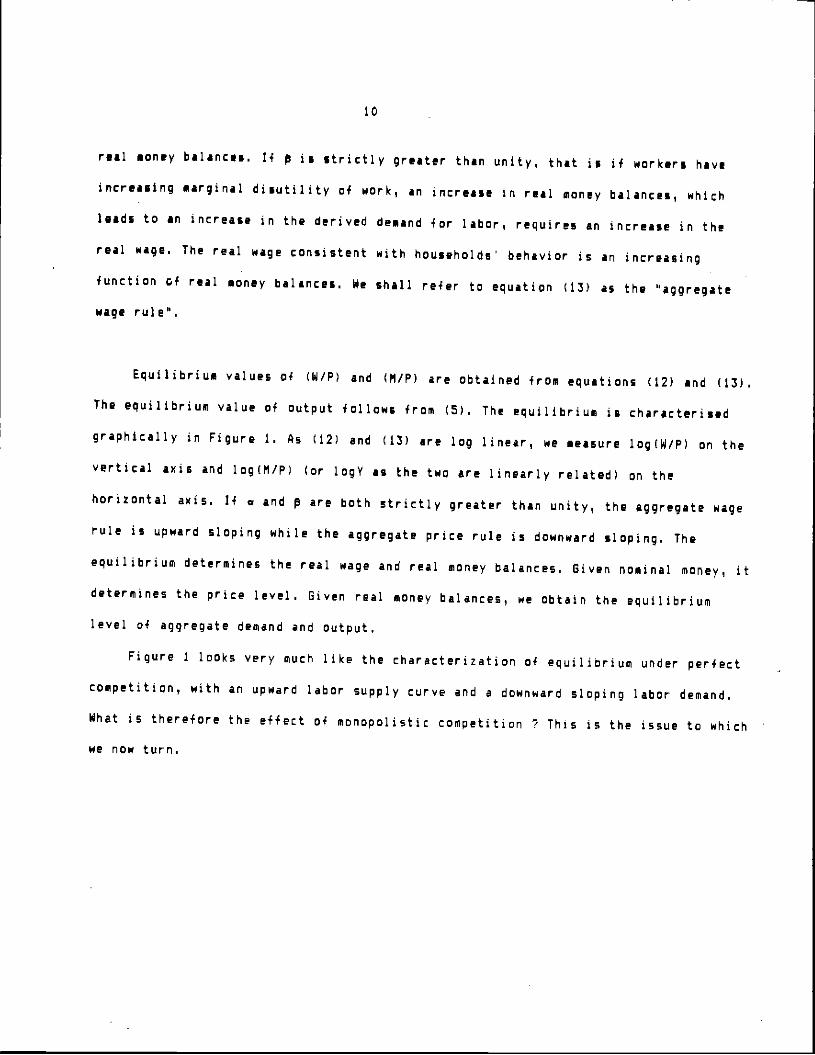
real money balances. 14 p ii strictly greater than unity, that is if workers have

increasing marginal disutility of work, an increase in real money balances, which

leads to in increase in the derived demand for labor, requires an increase in the

real wage. The real wage consistent with households' behavior is an increasing

function of real money balances. We shall refer to equation (13) as the "aggregate

wage rule.

Equilibrium values of (W/P) and (M/P) are obtained from equations (12) and (13).

The equilibrium value of output follows from (5). The equilibrium is characterised

graphically in Figure 1. As (12) and (13) are log linear1 we measure logcw/P) on the

vertical axis and log(M/P) (or logY as the two are linearly related) on the

horizontal axis. If a and p are both strictly greater than unity, the aggregate wage

rule is upward sloping while the aggregate price rule is downward sloping. The

equilibrium determines the real wage and real money balances. Given nominal money, it

determines the price level. Given real money balances, we obtain the equilibrium

level of aggregate demand and output.

Figure 1 looks very much like the characterization of equilibrium under perfect

competition, with an upward labor supply curve and a dDwnward sloping labor demand.

What is therefore the effect of monopolistic competition 7 This is the issue to which

we now turn.

Section 2 Inefficiency and externalities

Comparing monopolistic competition and perfect competition

lo characterize the inefficiency associated with monopolistic competition, we

first compare the equilibrium to the competitive equilibrium. The competitive

equilibrium is derived under the same assumptions about tastes, technology and the

number of firms and households, but assuming that each firm (each household) takes

its price (wage) as given when deciding about its output (labor).

The competitive equilibrium is very similar to the monopolistically competitive

one. The demand functions for goods and labor are still given by equations (7) and

(8). The price and wage rules are identical to equations (10) and (11), except for

the absence of 8/Ce—i) in the price rules and the absence of c/(u—i) in the wage

rules (the constant terms K, K,,, K,, K... and K are the same in both equilibria). (The

derivation is left to the reader). The explanation is simple. The term 61(9—1) is the

excess of price over marginal cost, reflecting the degree of monopoly power of firms

in the goods market if firms act competitively, price is instead equal to

cost. The same explanation applies to households.

Again, symmetry requires in equilibrium all nominal prices and all nominal wages

to be the saris this gives equations identical to (12) and (13), but without the

terms S/Cs—)) in the aggregate price rule and /(o'—i) in the aggregate wage rule. The

price wage ratio consistent with firms' behavior is lower in the competitive case by

9/CS—i) at any level of real money balances (output); the real wage consistent with

household's behavior is lower in the competitive case by u/Co—1) at any level of real

11

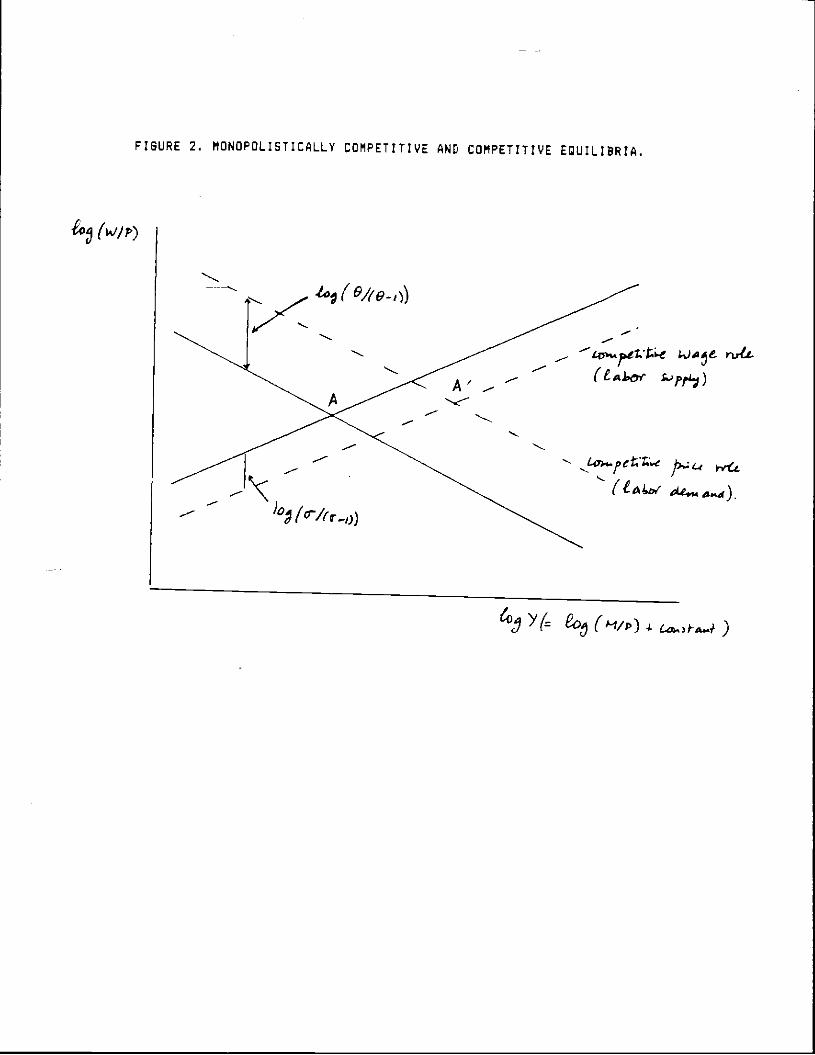
FIGURE 2. MONOPOLISTICALLY COMPETITIVE AND COMPETITIVE EQUILIBRIA.

— t.pett.e k)S1&nAt

£..'pØ)

(L4wAe...4._1)

4o (9,/(9,))

A'rI —

1°j fr/er_,

6j Y(= (Hip)

12

money balances. The monopolistically competitive and competitive aggregate wage and

price rules are drawn in Figure 2. Point A gives the competitive equilibrium, point

A gives the monopolistically competitive equilibrium.

The equilibrium level of real money balances is lower in the monopolistic

equilibrium the price level is higher. Employment and output are lower. What

happens to the real wage is ambiguous and depends on the degrees of monopoly power in

the goods and the labor markets. If, for example, there is monopolistic competition

in the goods market but perfect competition in the labor market, then the real wage

is unambiguously lower under monopolistic competition.

Denoting by R the ratio of output in the monopolistically competitive

equilibrium to output in the competitive equilibrium, R is given by

R o'—1 9-1 ) a-l 1

e 8

P is an increasing function of and 8. The higher the elasticity of

substitution between goods or between types of labor, the closer is the economy to

the competitive equilibrium. P is an increasing function of and . If and p are

both close to unity, P is small the existence of monopoly power in either the goods

or the labor markets can have a large effect on equilibrium output.

Aggregate demand externalities

Under monopolistic competition, output of monopolistically produced goods is too

low. We have shown above that this follows from the existence of monopoly power in

price and wage setting. n alternative way of thinking about it is that it follows

from an aggregate demand externality.

13

The argument is as follows i in the monopolistically competitive equilibrium,

each price (wage) setter has, given other prices, no incentive to decrease its own

price (wage) and increase its output (labor). Suppose however that all price setters

decrease their prices simultaneously p this increases real money balances and

aggregate demand. The increase in output reduces the initial distortion of

underproduction and underemployment and increases social welfare6.

We now make the argument more precise1 By the definition of a monopolistically

competitive equilibrium, no firm has an incentive to decrease its price, and no

worker has an incentive to decrease its wage, given other prices and wages, Consider

now a proportional decrease in all wages arid all prices, (dP./P1 ) (dW,/W) < 0 for

all i and i, which leaves all relative prices unchanged but decreases the price

level.

Consider first the change in the real value of firms9. At a given level of

output and employment, the real value of each firm is unchanged. The decrease in the

price level however increases real money balances and aggregate demand. This in turn

shifts outward the demand curve faced by each firm and increases profit an increase

in demand at a given relative price increases profit as price exceeds marginal cost.

Thus, the real value of each firm increases.

° An alternative way of stating the argument is as follows 14 startingfrom the monopolistically competitive equilibrium, a firm decreased its price,this would lead to a small decrease in the price level and thus to a smallincrease in aggregate demand. While the other firms and households wouldbenefit from this increase in aggregate demand, the original firm cannotcapture these benefits and thus has no incentive to decrease its price. Wehave chosen to present the argument in the text to facilitate comparison withthe argument of Section III.

What happens to the real value of firms is obviously of no directrelevance for welfare. This step is however required to characterize whathappens to the utility of household below.

14

Consider then the effect of a proportional reduction of prices and wages on the

utility of each household. Consider household j. We have seen that, once the

household has chosen the allocation of his wealth between real money balances and

consumption, we can write its utility as:

p(l1/P) —

where p is the constant marginal utility of real wealth and I. is the total wealth of

the Jth household. Using the budget constraint, we can express utility as

p a

IL, [j (W,/P)N — N 3 p E V±3/P + p (M3/P)i•1

Utility is the sum of three terms. The second is profit income —in terms of

utility— we have seen that each firms profit goes up after an increase in

aggregate demand. Thus, this term increases. The first term is the household

surplus from supplying labor. At a given level of employment, N, the proportional

change in wages and prices leaves this term unchanged. But the increase In aggregate

demand and the implied derived increase in employment implies that this term

increases : at a given real wage, an outward shift in the demand for labor increases

utility as the real wage initially exceeds the marginal utility of leisure. The third

term is the real value of the money stack, which increases with the fall in the price

level. Tnus, utility unambiguously increases.

10Note that, if we were performing the same experiment in the neighborood

not of the monopolistically competitive but of the competitive equilibrium,the first two terms would be equal to zero. The third one would however stilloe present. This is one of the implications of our use of real money as thenon produced good. If real money enters utility, then the competitiveequilibrium is not a Pareto optimum, as a small decrease in the price levelincreases welfare. This inefficiency of the competitive equilibrium disappearsf money is replaced by a non produced good, while the aggregate deamandexternality under monopolistic competition remains valid (see Kiyotaki 1994).

A similar point is made by Cooper and John C 1985].As we have not specified how money is introduced ir. this economy, it is

cest to think of them as helicopter drops.13 Here, and in the next section, instead of focusing on the effects ofaggregate aemand on output in general, we focus for convenience on the moreiarrow question of whether changes in nominal money have real effects. Theesults here and in the next section would apply equally to non monetary pureggreqate demand shifts, i.e. shifts which leave labor supply unchanged at auven real wage, where the real wage is defined as the aoe in terms of the:onsumption basket. If we modify the utility function to be

The notion of an aggregate demand externality is an old idea in macroeconomics.

It has been formalised in various recentpapers; although these papers have on the

surface relatively little in common, they share the following properties u an

increase in one agents activity increases the activity level and welfare of others

a general increase in activity, if it can be engineered, by taxation or other means,

may be welfare improving". Diamond (1982) builds a macroeconomic model where trade

takes place through search and shows that increased search by one trader has

externalities as it increases the probability for other traders to find a profitable

trade. Startz (1984) builds a macroeconomic model in which firms can not directly

observe effort by individual workers. This leads to a payment scheme which has the

implication that the optimal amount effort for each worker depends on the level of

effort put in by other workers. In both cases, a small increase in activity is

welfare improving.

Identifying the inefficiency associated with monopolistic competition as an

aggregate demand externality does not however imply that movements in aggregate

demand affect output. Consider for example changes in nominal money'2. As equations

(12) and (13) are homogeneous of degree zero in P, W and H, nominal money is

obviously neutral, affecting all nominal prices and wages proportionately and leaving

output and employment Thus something else is needed to obtain real

16

effects of nominal money. We examine tht effects of costs of price setting in the

next section.

1— p

U3 • (C3 )UM/P)+m) — N3 —p s

Then shifts in e will shift the demand for goods given real money balances,

while leaving labor supply unchanged at a given real wage and are thereforepure aggregate demand shocks. By contrast, shifts in are not pure aggregatedeamnd shocks.

17

Section 3. Menu costs and real effects of nominal tone

We now introduce small costs of setting prices, small "menu" costs. There are

obviously costs to changing prices, which range from the cost of changing tags and

printing new catalogs to gathering the information needed to choose the new prices,

informing new customers of these prices and so on. The question however is whether

these costs, which cannot be very large, can have important macroeconomic effects,

This section shows that theymay. Small menu costs may imply large movements in

activity in response to demand, and may have large welfare effects".

The first part of the section formalizes the argument for small changes in

nominal money, and shows the close relation between the aggregate demand externality

argument of the previous section and the argument presented in this section. The

second part considers larger changes in nominal money, and focuses on the effects of

structural parameters on the ratio of output and welfare effects to menu costs.

We are not the first to make this point. Ilankiw (1985) has pointed outthat, under imperfect competition! private and social costs of price setting could differsubstantially, leaving open the possibility of large welfare effects of demand changes.Akerlof and Yellen (l9BSa, 1985b) have emphasized the potential welfare effects of nearrationality under imperfect competition. Decision makers are said to be "near rational" ifthey react to changes in the environment only if not reacting would entail a first orderioss. As Akerlof and Yellen point out however, near rationality can be described as fullrationality subject to second order costs of taking decisions, so that their analysis isdirectly relevant to this section. Our contribution is to point out the relation to theaggregate demand externality emphasized in the last section, and because our model is moreexplicitly based on utility and profit maximisation, to give a more detailed welfareanal ysi S.

18

The effects of small changes in nominal money

We start by considering the effects of a small change in nominal money1 dM,

starting from the equilibrium described in the first section. The argument proceeds

as follows

At the initial nominal prices arid wages, the change in nominal money leads to a

change in aggrei'te demand, thus to a change in the demand facing each firm. If

demand is satisfied, the change in output implies in turn a change In the derived

demand for labor, thus a change in the demand facing each worker. Unless firms

operate under constant returns, each firm wants to change its relative price. Unless

workers have constant marginal utility of leisure, each worker wants to change his

relative wage. We show however that the loss in value to a firm which does not adjust

its relative price is of second order ; the same is true of the utility of a worker

who does not adjust his relative wage. Thus second order menu costs may prevent firms

and workers from adjusting prices and wages. The implication is that nominal prices

and nominal wages do not adjust to the change in nominal money. The second part of

the argument is to show that the change in real money balances has first order

effects on weifare we show that the effect on welfare is indeed first order, and of

the same sign as the change in money. The argument has very much the same structure

as the aggregate demand externality argument of the previous section ; this

coincidence is not accidental and we return to it below.

The first part is a direct application of the envelope theorem. Consider firms

first. Let V1 be the value of firm i. V± is a function of P± as well as of P, W and II

V1 = V1 (Pi ,P,W,tl) . Let V1 — be the maximised value of firm i, after maximisation

over P1 V = V(P,W,M) . The envelope theorem then says that

FIGURE 3. AGGREGATE DEMAND EXTERNALITIES AND MENU COSTS

(Pin)

t.og(iii)

& (P/n')

0

&1O1H)

r &dct A

E1 (P/ri

a—il-c j—c}V

/ oj

19

dV./dM • 8V1/IM + (6V,I8P) (dP./dPl) • 8V,/SM

To a first order, the effect of a change in Fl on the value of the firm is the

same whether or not it adjusts its price optimally in response to the change in P1.

Exactly the same argument applies to the utility of the household. Thus, second order

menu costs (but larger than the second order loss in utility or in value) will

prevent each firm from changing its price given other prices and wages and each

worker from changing its wage given other prices and wages. The implication is that

all nominal prices and wages remain unchanged and that the increase in nominal money

implies a proportional increase in real money balances.

What remains to be shown is that the change in real money balances has positive

first order effects on welfare. }owever, as we have already shown in the previous

section, the increase in real money balances, associated with the increase in

aggregate demand and employment, raise; firmsprofits and the households' surpluses

from supplying labor. Thus, it increases welfare in the neighborood of the

monopol i stically competitive equilibrium.

The relation between aggregate demand externalities and the argument of this

section is illustrated using the diagram in Figure 315•

Figure 3 plots the price rule (10) giving the price chosen by firm i as a

function of the price level. The logarithm of the price level is on the vertical axis

while the logarithm of the price of the it' firm is on the horizontal one both are

The reason why the argument below is only an illustration is that it only looks atfirms, taking the real wage as given it is thus only a partial equilibrium argument. Thergument would be a general equilibrium one if we were looking at an economy composed ofouseholds, each producing a differentiated good.

20

measured as ratios to nominal money. The price rule is drawn for a given real wage

(WIN (assumed to be set at its monopolistically competitive value) and gives

log(P/K) as a linear function of logCP/P'l). in the presence of monopoly power, the

price rule has slope greater than one. We also drawisoprofit loci, giving

combinations of (P,/M) and (PIM) which yield the same level of real profit for the

firm''. The symmetric monopolisticallycompetitive equllibriu& is given by the

intersection of the price rule and the 45 degree line, point E. Point A gives the

highest real profit point on the 45 degree line.

The aggregate demand externality argument can then be stated as follows.Consider a small proportional decrease of

prices, keeping nominal money and the real

wage constant. The equilibrium moves from paint E to a point like E along the 45

degree line. The profit of each firm rises with the increase in aggregate demand.

However, in the absence of coordination, no firm has an incentive to reduce prices

away from the equilibrium point E.

The menu cost argument considers instead a small increase in nominal monet. At

the initial set of prices, realmoney balances would increase and the economy would

move from point E to a point like point E . But, absent menu costs, each firm would

find in its interest to increase itsprice until the economy had returned to point E.

In the presence of menu costs however, thesemenu costs, if large enough, can prevent

this movement back to E, so that the economy remains at E and all firms end up with

higher real profits.

The figure assumes decreasing returns to scale. Note also that, as firms take thePrice level as given when choosing their own price, isoprofit loci are horizontal alongthe price rule.

21

P similar argument, although slightly more complicated, holds for wages. We

shall not present it here.

it is also important to note the specific role pyd by mony in this section.

The presence of an aggregate demand externality does not depend on the nature of the

produced good, and on the nature of the numeraire. The results of this section depend

on money being the non produced good and the numeraire, That money is the numeraire

implies that, given menu costs, unchanged prices and wages mean unchanged nominal

prices and wages. That money is the non produced good implies that as the government

can vary the amount of nominal money, it can, if nominal prices and wages do not

adjust, change the amount of real money balances, the real quantity of the non

produced good.

The effects of iaroer chanoes in nominal money

If we want to examine the effects of larger changes in nominal money, we can no

longer use the result derived above, for its proof relies on the assumption of small

changes in money. For larger changes, the private opportunity costs of not adjusting

prices in response to the change in money —private costs, for short— are no longer

negligible and depend on the parameters of the model. We now investigate this

dependence.

The private costs laced by a firm depends on the size of the demand shifts as

well as on the two parameters and 9. As we have seen, these costs are of second

order in response to a change in aggregate demand, thus roughly proportional to the

square of the change in aggregate demand. More precisely, define NA p ,$) to be the

private opportunity cost to a firm expressed as a proportion of initial revenues,

associated with not adjusting its price in response to a change of IOOA% in aggregate

22

demand, when all other firms and households keep their prices and wages unchanged.

Then, by simple computation, we get

L (A m,9) (C ( — 1)2(9I)]/ 12(1+9(—1))]) A' + o(A2)

where o(A2) is of third order.

The closer - i s to one , i • e the closer to constant returns are the returns to

scale, the smaller the private cost. In the limit, if is equal to one, then private

costs of not adjusting prices are equal to zero as the optimal response of a

monopolist to a multiplicative shift in isoelastic demand under constant marginal

cost is to leave the price unchanged. Thus private costs are an increasing function

of . They are also an increasing function of 9 the higher the elasticity of demand

with respect to price, the higher the private costs of not adjusting prices.

Ewactly the same analysis applies to workers. The two important parameters for

them are and o, If we define the function L in the same way as above, the private

opportunity cost to a worker, measured in terms of consumption and expressed as a

proportion of initial consumption), associatet with not adjusting the waqe in

response to a change of lOOM, in aggregate demand, when all other firms and

households keep their prices and wages unchanged, is given by

C (9—1)J9] L( (1+A) —1

where (9—1)I9 is the initial share of wage income in BNP.

If is close to unity, i.e if the elasticity of the marginal disutility of

labor is close to unity, private costs of not adjusting wages are small ; in the

limit, if marginal disutility of labor is constant, private costs are equal to zero.

If is very large, if labor types are close substitutes, private costs of not

adjusting wages are high.

23

Table Ia gives the size of menu colts as a proportion of the firms revenues

(GNP produced by the firm) which are just sufficient to prevent a firm from adjusting

its price in response to a change in demand Table lb gives the size of menu costs

(in terms of consumption) as a proportion of initial consumption (GNP consumed by the

worker) which are just sufficient to prevent a worker from adjusting his wage. --

Lbie I Changes in agQgate demand and menu costs(a) (b)

Loss in value to a firm from not Loss in utility (in terms of consumptiDn)adjusting prices (as a proportion to a worker from not adjusting wages asof initial revenues) a proportion of initial consumption)*

alpha theta 1.05 1.10 beta sigma 1.05 1.10

1.1 5 .003% .013 1.4 5 .0667. .265

1.1 2 .001 .004 1.4 2 .027 .11120 .008 .031 20 .105 .416

1.0 5 .000 .000 1.2 5 .025 .1001.3 5 .018 .071 1.6 5 .112 .451

* e 5 a 1.1

N0 is the initial level of nominal money, H, the level after the change.

Thus, given the unit elasticity of aggregate demand with respect to real money

balances and the assumption that all other prices have not changed, table Ia gives

the private costs associated with not changing prices in the face of 57. and lox

changes in demand to the firm. The main conclusion is that very small menu costs ,say

less than .017. of revenues, may be sufficient to prevent adjustment of prices.

Results are qualitatively similar for workers. Table lb gives the private costs of

not changinc the effects of changes of +57. and +107. in the demand for final goods. It

24

assumes that is equal to 1.1, so that changes in the der2ved demand for labor are

of 5.5% and 11% approximately. Weexpect p to be higher than so that table lb looks

at values of p between 1.2 and 1.6. For values of p close to unity, required menu

costs are again very smallas p increases however, required menu casts become non

negligible for and a 11% change in demand, they reach .45% of initial

consumption, a number which is no longer negligible.

The more relevant comparison however, at least from the point of view of

welfare, is between private costs and welfare effects, i.e. the change in utility

resulting from the changes in output, employment andreal money which are implied by

a change in nominal money at given prices andwages. Welfare effects depend on the

size of the change in nominal money as well as on the parameters a1 1 and op the

dependence is a complex one and we shall not analyze it here in detail, Table 2 gives

numerical examples. It gives the required menu costs and welfare effects associated

with two different changes in nominal money, 5% and 10% and different values of the

structural parameters.

For each of the two changes inmoney, the first column gives the minimum value

of menu costs, expressed as a proportion of GNP, which prevents adjustment of nominal

prices and wages ; this value is the sum of menu costs required to prevent firms from

adjusting their prices and workers from adjusting theirwages, given other wages and

prices. The second column gives the welfare effects of an increase in nominal money

at unchanged prices and wages, expressed in terms of consumption, again as a

proportion of GNP. The third gives the ratio of welfare effects to menu costs.

25

Table 2 Menu costs and welfare effects

1.05 M1/N0 = 1.10

alpha beta Menu Welfare Ratio Menu Welfare RatioCosts Effects Costs effects

(eu5)1.1 1.2 .03% 1.797. 60 .11% 3.54% 32

1.4 .07% 1.83% 26 .28% 3.60% 131.6 .11% 1.91% 17 .46% 3.72% 8

1.2 1.2 .04% 1.62% 45 .15% 3.57% 241.4 .08% 1.877. 24 .33% 3.67% Ii

1.6 .13% 1.98% 15 .53% 3.65% 7

($.o.10)1.1 1.2 .03% .94% 31 .11% 1.86% 17

1.4 .06% 1.02% 17 .23% 1.93% 81.6 .09% 1.11% 12 .36% 2.05% 6

1.2 1.2 .04% .99% 25 .16% 1.87% 121.4 .07% 1.07% 16 .29% 2.01% 71.6 .11% 1.27% 12 .44% 2.24% 5

Welfare effects turn out not to be much affected by the specific values of the

parameters, at least for the range of values we consider in the table. Thus, the

ratio of welfare effects to menu cost has the same qualitative behavior as that of

the ratio of output movements to menu costs. It is largest for values of m, p, $ and

a close to unity, and decreases as these parameters increase. In the table, it varies

from 60 for low values of m p, S and to 5 for high values of these parameters.

Demand determinationofoup

We have until now assumed that increases in real money balances at constant

prices and wages led to increases in output and employment. When we were analyzing

the effects of small changes ir money, this assumption was clearly warranted in the

-io (k'/p)

0

FIGURE 4. DEMAND DETERMINATION OF OUTPUT.

fr';c:, yjt,

-

V= (i,)* C)M)

26

initial conopolistically competitive equilibrium, as price exceedE marginal cost,

firms will always be willing to satisfy a small increase in demand at the existing

price. The same is true of workers as the real wage initially exceeds the marginal

disutility of labor, workers will willingly accomodate a small increase in demand for

their type of labor. When we consider larger changes in money, this may no longer be

the case. Even if firms do not adjust their price, they have the option of either

accomodating or rationing demand ; they will resort to the second option if marginal

cost exceeds price. The same analysis applies to workers. From standard monopoly

theory, we know that firms and workers will accomodate relative increases in demand

of

IL Iand (o/(e—1))p—1 respectively

This raises the question of whether, assuming menu costs to be large enough, an

increase in demand can increase output all the way to its competitive level. The

answer is provided in Figure 4. Figure 4 replicates Figure 2 and draws the aggregate

price and wage rules under competitive and monopolistically competitive conditiDns. A

is the monopolistic competitive equilibrium, A' the competitive one. Along the

monopolistically competitive price rule, price exceeds marginal cost thus firms

will satisfy demand, at a aiven price wage ratio, until marginal cost equals price,

that is until they reach the competitive locus, In our case, firms will supply up to

point B. The shaded area F is the set of output—real wage at which firms will ration

rather than supply. By a similar argument, workers will supply up to point B • The

shaded area N is the set of real wage combinations where workers do not satisfy labor

demand. The figure makes it clear that an increase in nominal money will increase

output and employment. It also makes clear that, no matter how large menu costs are,

27

it is impossible unless the competitive andmonopolistically competitive real wages

are equal, to attain the competitive equilibriumthrough an increase in nominal

money.

What happens therefore as demand increase; depends on both menu casts and supply

constraints. If menu costs are larae, supply constraints will come into effect first.

If menu costs are small a more likely case, prices and wages adjust before supply

constraints come into effect.

Conclusion

The results of this paper are tantalizingly close to those of traditional

Keynesian models under monopolistic competition, output is too low, because of an

aggregate demand externality. This externality, together with small menu costs,

implies that movements in demand can affect output and welfare. Inparticular,

increases in nominal money can increase both output and welfare, In fact, while we

believe these results to be important to the understanding of macroeconomic

fluctuations, it is also clear that there is still a long way to go for this model to

Justify Keynesian results. Let us mention some of the main issues.

The scope for small menu costs to lead to large output, employment and welfare

effects in our model depends critically on the elasticity of labor supply with

respect to the real wage being large enough (on (—l) being small). Evidence or

individual labor supply suggests however a small elasticity, Thus the 'menu cost"

approach runs into the same problem as the imperfect information approach to output

fluctuations neither can easily generate large fluctuations in output in response

to demand if the real wage elasticity of labor supply is low. As ir, the imperfect

information case, the theory may be rescued by the distinction between temporary and

28

permanent changes in demand. An other possibility is that unions have a flatter labor

supply than individuals. More likely, the assumption that labor markets operate as

spot markets (competitive or monopoflstically competitive) may have to be

abandoned''.

The ana'ysis of this paper is purely static. There are substantial conceptual

issues in extending the model to look at the dynamic effects of demand on output, in

the presence of menu costs, If menu costs lead to staggered nominal price and wage

decisions, with fixed lengths of time between decisions, the model delivers1

depending on the particular staggering structure, the same qualitative results as

recent macroeconomic models with staggering, such as those by Akerlof (L969), Taylor

(1979) and Slanchard (1983) (see Blanchard (1985) for a more detailed argument). if

however menu costs lead price and wage setters to use (S,s) policies, which imply

random periods of time between decisions, the results may be quite different p in

response to a change in aggregate demand, only a few prices may be readjusted p they

may however be readjusted by a large amount, implying a large change in the price

level, and little effect of real money on output, apart form the distortions on the

price structure (see Caplin and Spulber (1985), and Blanchard and Fischer (1985) for

further discussion),

'' This is the direction taken by Akerlof and Vellen (1985b) who formalize the goodsmarket as monopolistically competitive and the labor market using the 'efficiency wage"hypothesis.

Appendix

This appendix derives the market equilibrium conditions (5) to (11)

given in the text and proceeds in three steps. The first derives the demand

functions of each type of )abor and each type of product by solving part of

the maximization problems of firms and households. These functions hold

whether or not_prices and wages are set by workers and firms at their profit

or utility maximizing level. The second derives price rules from firms

profit maximization and wage rules from workers utility maximization. The

third characterises market equilibrium.

1. Demands for product and labor types

a) in order to maximize profit, each firm minimizes its production costfor a given level of output and wages

n n I

sin W N1 subject to ( E NT)3d j1

Solving this minimimation problem gives i

-aN1 (n T1 (W3/W) Y

n 1

and E W N U- 1—a) W Y (allj=j

-

n 1—a 1

where W ((I/n) W 11—a (a2)1The demand for labor of type 3 is therefore given by

—a

= E Nj = (W3/W) N/n (a3)i =1

mn 1 m

where N E CE E W N±)/W (n 1—o') V1 (a4)i .1 1=1

N can be interpreted as the aggregate labor index

bI in order to maximize utility, each household chooses the optimumcomposition of consumption and money holdings for a giver level of totalwealth Ii and product prices

s—i or

max A3 ( t C18 )€+—l(M3/P)

ifsubject to E P± C + N3 I.,

1=1

Solving this maximization problem gives i—8

• (P./P) U Ij/Pm) (a5)

P13 (I—fl I and (a6)

A3 i 11/P (a?)if i—s i I r

where P ((i/rn) E F, ) 1—6 and p • (1 m 8—1) (1—1) CaB)

p can be interpreted as the marginal utility of real wealth

The demand for product of type i is therefore given by—e

Vt = E = (F'1/P) (Vim) (a9)1=1

n if n

where V = CE E P± C.3)/P (l/P) E I. (alO)

j i jal

V denotes real aggregate consumption expenditures of households and willbe referred to as "aggregate demand",

Note that (a5) , (a6) (a9) and (alO) imply the following relationbetween aggregate demand and aggregate desired real money balances

n

V = (11(1—fl) N/P where Fl= E N'3 (all)j=l

2. Price and waoe rules

a) Taking as given waaes and the price level1 each firm chooses itsprice and output so as to maximize profit

V1 = P. V1 — (43 N3 (a12)

j=1

subject to the cost function Cal) and the demand function for itsproduct (a9). Salving the above maximization problem gives

1 cr1= (8/48—iHn 1—c a V± (4, or equivalently (a13)

1a cr1 1

P1 /P [((8/ (8— 1)) n i—c m ) ((4/F') (V ) 1 (1±6 (cr-I) ) (a 14)

Equation (all) Implies that the price is equal to 91(6—1) times the

b) Taking as given prices and other wages, each household chooies itswage and labor supply so as to maximize utility. Using (*6)

u

• p li/P — N

subject to the demand forconstraint i

its type of labor (a3) and the budget

W N + E +

Solving this maimization problem givesi

p Wi/P = (u/(o—l)) N ,or equivalently

(a 16)

W,/W IC (a/(c—1) ) (/p)n1—a 6-1 1

)(P/W)(N )J (l+o(—1))

Equation (aiB) implies that the real wage1 In terms of utility, is equalto a/Cu—i) times the marginal disutility of labor.

3. Market equilibrium

In equilibrium, desired real money balances must be equal to actualbalances. Thus P1 P1'. Replacing in Call) gives

= (rI(1—)) P1/P

This is equation (5) in the text. Then, from equations (a4), Ca9) and

i =1

If all firms choose the same —not necessarily optimal— price, thisreduces to

Substituting equationproduct i, equation (7) inequation (a3) gives thethe text. Note that asthese demand functions,

optimally.Substituting equation

equation (10) in the text,for worker i, equation (11)

marginal cost

(a1)

(a 17)

(ale)

(a19) , we get

N = tin 1—a) (XI(1—)) m

(a 19)

m -o6

E (P1/N ) (HIP)

_L_ 1'0( U

N En 1— m U/Cl—fl)) (HIP)

(a20)

(a21

(a19) into (a?) gives the demand function forthe text. Substituting equation (a21) into

demand function for labor of type .i, equation (B)we have not used the price and wage rules to derivethey hold even when prices or wages are not set

(a19) into (a14) gives the price rule for firm i,Substituting (a19) into (alS) gives the wage rulein the text.

in

BIb 11 ography

Akerlol, Beorge, "Relative wages and the rate of inflation", OlE 83—3 (August1969) : 353—374

Akerlof, George and Janet Yellen, "Can small deviation! from rationality makesignificant differences to economic equilibria?', AER, 75—4

(September 1985,a)706—721

Akerlof, George arid Janet 't'ellen, "A near—rational model of the business cycle,with wage end price inertia", forthcoming OJE, 1985,b

Ellanchard, Olivier, "Price asynchronization and price level inertia", in"Indeation, Contracting and debt in an inflationary world", Dornbusch and Simonseneds, MIT press, 1983 : 3—24

Blanchard, Olivier, "The wage price spiral", forthcoming QJE, 1985

Blanchard, Olivier and Stanley Fischer, "Macroeconomics", Chapters Band 9,mimeo 1985

Caplin, Andrew and Daniel Spulber, "Menu costs, inflation and endogenousrelative price variability", mimeo, Harvard, 1965

Cooper, Russell and Andrew John, "Coordinating coordination failures InKeynesian models", mimec, Cowles Foundatiori,745, April 1985

Diamond, Peter, "Aggregate demand management in search equilibrium", JPE, 90,October 1982 : 881—894

Dixit, Avinash and Joseph Stiglitz, "Monopolistic competition and optimumproduct diversity", PER, 67—3, June 1977, 297—308 -

Hart, Oliver, "A model of imperfect competition with Keynesian featuresH, OJE97—1 (February 1982) :109—138

Kiyotaki, Nobuhiro, "Macroeconomic implications of monopolistic competition",mimeo Harvard, April 1984

Mankiw, Gregory, "Small menu costs and large business cycles : a macroeconomicmodel of monopoly", OJE, 100—2 (May 1985) : 529—539

Mortensen, Dale1 "The matching process as a non cooperative bargaining game", in"The economics of information and uncertainty", John McCall ed, University of ChicagoPress and NBER, 1982

Solow, Robert, "Monopolistic competition and the multiplier", mimeo MIT, 1984

Startz, Richard, "Prelude to macroeconomics", AER, 74, (December 1984) : 881—892

Taylor, John, "Staggered price setting in a macro model", PER 69—2 (May 1979):108—113