NBER WORKING PAPER SERIES

EXISTENCE AND PERSISTENCE OF PRICE DISPERSION: AN EMPIRICAL ANALYSIS

Saul Lach

Working Paper 8737http://www.nber.org/papers/w8737

NATIONAL BUREAU OF ECONOMIC RESEARCH1050 Massachusetts Avenue

Cambridge, MA 02138January 2002

I thank David Genesove, Kala Krishna and Shlomo Yitzhaki for their comments and Aryeh Bassov forexcellent research assistance. I also thank the Central Bureau of Statistics in Israel for making the price dataavailable for research. Financial support from the Israel Science Foundation and from the Morris FalkInstitute for Economic Research in Israel is gratefully acknowledged. The views expressed herein are thoseof the author and not necessarily those of the National Bureau of Economic Research.

© 2002 by Saul Lach. All rights reserved. Short sections of text, not to exceed two paragraphs, may bequoted without explicit permission provided that full credit, including © notice, is given to the source.

Existence and Persistence of Price Dispersion: an Empirical AnalysisSaul LachNBER Working Paper No. 8737January 2002JEL No. L11

ABSTRACT

Using a unique data set on store-level monthly prices of four homogenous products sold in Israel,

I study the existence and characteristics of the dispersion of prices across stores, as well as its persistence

over time. I find that price dispersion prevails even after controlling for observed and unobserved product

heterogeneity. Moreover, intra-distribution mobility is significant: stores move up and down the cross-

sectional price distribution. Thus, consumers cannot learn about stores that consistently post low prices.

As a consequence, price dispersion does not disappear and persists over time as predicted by Varian�s

(1980) model of sales.

Saul LachDepartment of EconomicsHebrew UniversityJerusalem, 91905Israeland NBERSaul.Lach@huji.ac.il

1 Introduction

Casual observation indicates that price dispersion is a readily observed feature of many markets:

deviations from the “law of one price” are the norm, rather than the exception. Indeed, a

variety of models have been developed in the Industrial Organization literature to account for

this fact. It is therefore surprising that price dispersion has not been the subject of a rigorous

and systematic empirical scrutiny: we do not have a clear sense of the magnitude of price

dispersion nor of its relationship to the type of product, and we know even less about the

reasons for its existence.

Indeed, since the seminal work of Pratt, Wise and Zeckhauser (1979) there has not been

much empirical work documenting the extent and types of price dispersion. Lack of adequate

data is probably the main reason for this dearth of empirical work.1 In this paper, I use unique

data on store-level prices of four homogenous products sold in Israel to study the existence and

characteristics of the dispersion of prices across stores, and its persistence over time.

Many of the theoretical models on price dispersion are static by nature: they analyze a

single-shot pricing game between firms selling the same good. Cross-sectional price dispersion

is the result of a Nash equilibrium in pure or in mixed strategies (prices). In the pure strategy

case, some stores persistently sell their product at lower prices. If consumers can learn from

experience, this persistence seems rather implausible to sustain over time. In the mixed-strategy

case, stores randomize their prices and, therefore, do not post consistently low or high prices. As

a consequence, consumers cannot learn about stores that consistently have low prices (Varian,

1980). Hence price dispersion does not disappear and may be expected to persist over time.

This reasoning implies that if price dispersion is persistent, the ranking of stores in the

price distribution should fluctuate over time. Giving empirical content to this hypothesis, and

testing it with the available data, is the second goal of this paper. To the best of my knowledge

this is the first empirical study to analyze the evolution over time of the price distribution with

micro-level data. This is now feasible because, for each product, I have a long time-series of

monthly price observations by store.

The main result is that price dispersion across stores is prevalent and differs across prod-

ucts in reasonable ways. Price dispersion prevails after controlling for observed and unobserved

product heterogeneity. In addition, intra-distribution mobility is significant: stores move up

and down the cross-sectional price distribution. Thus, consumers cannot learn about which

1There is, however, some empirical work in the marketing literature based mostly on ad-hoc survey data.Pratt, Wise and Zeckhauser (1979) collected their own price data from stores selected from the Boston YellowPages.

1

stores have consistently low prices.

The paper is organized as follows. After a brief theoretical background in Section 2

and a description of the data in Section 3, the existence and characteristics of price dispersion

are examined in Section 4. In Section 5, I analyze the extent of intra-distribution mobility.

Conclusions close the paper.

2 Theoretical Background

The theoretical literature on price dispersion offers a variety of models with non-degenerate

price distributions as the equilibrium outcome: stores charge different prices for the same ho-

mogenous good. These models then rationalize the observed price dispersion as an equilibrium

phenomena.

In a world with identical sellers and buyers and with perfect information (alternatively,

when consumers can search costlessly for the lowest price) and no capacity constraints, the

unique Nash equilibrium is the perfectly competitive price (the Bertrand outcome). On the

other hand, imperfect information is not sufficient to support price dispersion. If search costs

are strictly positive the unique equilibrium is the monopoly price (Diamond, 1971). Imperfect

information makes it possible for firms to “capture” customers and act as local monopolists

because consumers must incur positive costs of finding lower prices.

The message from the Diamond model is that for price dispersion to exist in equilibrium,

there must be some heterogeneity among buyers and/or sellers.2 For example, when a mass

of consumers have negligible search costs, they will eventually get informed about the stores

charging the lowest price. These consumers are the “shoppers”. It then pays to deviate from

the monopoly price because stores that deviate will get all the shoppers. In equilibrium, the

shoppers will pay a low price, while the remaining consumers shop randomly and will pay either

the low or the high price.

Products that are otherwise homogenous are sold by different sellers and some of this

heterogeneity is passed on to the products turning them, in fact, into “differentiated products”.

In the classical models of Hotelling (1929) and Chamberlin (1933), products differ in their

2Different models emphasize different sources of heterogeneity. For example, price dispersion may arisebecause of differences in the sellers’ production costs (Reinganum, 1979), differences in consumers’ search costs(Rob, 1985), or in their beliefs about the price distribution (Rothschild, 1974), differences in the repetitiveness ofpurchases and resultant customer loyalties (McMillan and Morgan, 1988), and differences in buyers’ informationabout prices due to their random exposure to advertising (Butters, 1977). Even when consumers and firmsare identical ex-ante, a price dispersion equilibrium can arise as a result of ex-post heterogeneity in the priceinformation consumers receive (Burdett and Judd, 1983). Note that in all these models the heterogeneity pertainsto the buyers and/or to the sellers. It is therefore not that surprising that the equilibrium price distributionreflects this underlying heterogeneity.

2

location only. In these models also, product differentiation leads to monopolistic competition

and, consequently, to price dispersion.

Finally, if price dispersion for an homogeneous product is to persist over time, the equi-

librium price choices cannot be a pure strategy equilibrium. If some stores are always selling at

low prices, and if consumers can learn over time to identify these stores, then they will eventu-

ally shop at the low-priced stores and price dispersion will tend to disappear. If the dispersion

in prices persists over time then it must be that sellers vary their prices randomly over time

so that consumers cannot fully learn which store is selling at the lowest price, a point argued

forcefully by Varian (1980). The use of mixed strategies—sales—carries the empirical implication

that the position of the store (ranking) within the cross-sectional price distribution changes

over time in a random fashion.

In sum, theory tells us that lack of full information and some heterogeneity in the buyers

and/or sellers, which may be passed on to the products, is necessary for price dispersion to

exist. Furthermore, for price dispersion to persist over time, sellers should be changing their

prices (randomly) so as to preclude consumers from getting fully informed.

3 The Data

The data set consists of price quotations obtained from retail stores by the Central Bureau of

Statistics (CBS). Once a month, the CBS samples prices on a variety of goods from a sample

of stores, and uses them to compute the monthly Consumer Price Index.3

I originally collected data on 31 products for the period January 1993—June 1994 (18

months). These products were selected after reviewing the list of major items in the CPI for

goods having a precise label that make them easily identifiable by the person collecting the

price data at the store. This should ensure that the prices over time correspond to the same

physical product. For example, I chose a product labeled “Brand A Instant Coffee (250 grams)”

but would not have selected it if, instead, it were labeled just “Brand A Instant Coffee”. In

many cases, price quotations of different brands are obtained in different stores and I know

which store is quoting which branch of the product.4

Many of these products, however, have relatively small number of stores with price

3 Importantly, the price data are not “scanner” data. The prices are therefore “asking” prices. For manyproducts, asking and actual transaction prices are identical. The data set used by Lach and Tsiddon (1992,1996) came from the same source (the CBS), but included different products and covered a different time period.

4For example, store 1 quotes the price of a bottle of brand A beer and store 2 quotes the price of a similarsized bottle of brand B beer. In general, the brand quoted at the store does not change during the sample period.

3

quotations in any month (less than 7-8 stores), making the estimates of price dispersion for

these products not very reliable. I therefore decided to focus on just four products with a

relatively large number of stores per month. For these products, the time series data were

extended until December 1996, totalling 48 months of price quotations. The list of products

appears in Table 1.

There is one durable good—a refrigerator—and three frequently purchased food staples—

chicken, coffee, and flour. In any given month (out of the 48 months) there are at least 35 stores

with price data on the refrigerator, but no more than 43 stores. On average, in any month,

I have price data from 38 stores selling the refrigerator, and from 37 stores selling chicken,

but only from about 14-15 stores selling coffee tins or flour packages. This results in that the

number of observations for the refrigerator and the chicken products is 2-3 times larger than

that for coffee and flour.

There is variation in the number of reporting stores over time because the sample of

stores changes slowly over time (new stores are added to the sample while others drop out)

and also because stores that are out of stock when visited by the CPI surveyor are assigned a

missing value.5 On average, a store appears in the sample, i.e., has a price quotation, in over

75 percent of the sample period (in 37-40 out of the 48 months).

As mentioned above, the definition of the products is very precise and includes the brand

name, weight, model number, and other identifying information ensuring that the prices refer

to the same product across stores. The refrigerator, coffee and flour are exactly the same

product in terms of physical attributes (brand, model, size, etc.). In short, these products are

“homogenous” as far as physical characteristics go.

The price of the chicken product refers to 1 kilogram of a whole frozen chicken. Re-

gretfully, there is no information on the specific brand quoted by the store. Frozen chicken,

however, is most likely a “generic” product because customers do not care (much) about the

brand.6 Frozen chicken comes in three sizes and I do have this information. Because size may

affect the price per kilogram I will control for this size effect when comparing prices across

stores. In any case, over 2/3 of the observations correspond to the smallest-sized chicken (Size

1).7

5This does not occur very frequently. When the prices in the months preceding and following a month witha missing value remained constant, that constant price was imputed to the month having the missing value.

6From casual observation. Moreover, one brand dominates the market so that most quotations probably referto the dominating brand.

7The largest sized chicken is sold in only one store in the sample. 69 percent of the observations correspondto the smallest chicken (Size 1) while 29 correspond to the intermediate size (Size 2).

4

This concern for preserving homogeneity of the product across stores and over time

makes these data uniquely suited for the measurement and analysis of price dispersion. When

consumers buy many products at the same store, the prices of the various products sold by

the retailer are interdependent (Lal and Matutes, 1989). In this setting, one may naturally

be interested in the price dispersion of baskets of products across stores or, more generally, on

properties of the joint price distribution of many products. The available data do not allow me

to tackle this issue. I focus, instead, on the marginal price distributions, and their associated

dispersion measures, of the four products. These marginal distributions arise naturally in

models of equilibrium price dispersion in multiproduct settings (McAfee, 1995; Gatti, 2000).

4 Estimates of Cross-Sectional Price Dispersion

Because the general price level increased at an annual rate of about 10-12 percent during 1993-

96, nominal prices were transformed into real prices by dividing each price quotation by the

CPI monthly index. Henceforth, all prices are in terms of January 1993 prices in New Israeli

Shekels (NIS).8

4.1 Preliminary Estimates

Figure 1 displays kernel estimates of the log price distribution pooled over stores and months.

Log prices are expressed as deviations from the month’s average. Because adjusted log prices av-

erage to zero in every month all the variation in the densities is within-month (cross-sectional).

Obviously, the notion of “one price” does not hold in the data. In fact, prices exhibit

substantial dispersion. Table 2 presents simple means and variation measures of the real price

data (not in logs nor in deviation terms). Averaging over months and stores, the mean price

of the refrigerator during the four-year period was 3170 NIS with a standard deviation of 154

NIS. A kilogram of frozen chicken and coffee had comparable mean prices while flour was an

order of magnitude cheaper.

The relationship between price dispersion and the type of product is interesting. Figure

1 and all the dispersion measures in Table 2 indicate that the refrigerator is the product with

the lowest price dispersion, while coffee exhibits the highest price dispersion. In fact, 50 (90)

percent of the refrigerator price quotations in the middle of the distribution are within 5 (15)

percent of each other. Given that a reasonable discount is about 5-10 percent of the price,

refrigerator prices are tightly concentrated in this region of the distribution. Nevertheless,

8The exchange rate in January 1993 was 2.76 NIS per U.S. dollar.

5

prices are dispersed: the highest price is 43 percent higher than the lowest one. In the three

food products, the mid-50 percent of the prices are much more dispersed, and the highest price

is more than twice the lowest price.

In their sample, Pratt, Wise and Zeckhauser (1979) found that the coefficient of variation

decreases with the mean price of the good. Table 2 reports a similar finding. These results

are consistent with the view that, because of the presence of a fixed cost component, search is

more valuable for high-price goods. In other words, search costs are low relative to the high

price of the good and, as a consequence, more searching for the lowest price is undertaken.

Eventually, consumers will get fully informed about which store is charging what price. Stores

will then have to price at approximately the same marginal cost—the Bertrand outcome—and

exhibit minimal price dispersion in equilibrium. On the other hand, in the case of low-price

items, search costs relative to the price of the good may be significant for some consumers and

these will refrain from a complete search for the lowest price. An equilibrium can then exist

in which consumers with high search costs pay higher prices than consumers with low search

costs—the shoppers—resulting in price dispersion.9

4.2 Heterogeneity-controlled Estimates

Even though the products appear homogenous in terms of physical characteristics, all four

products are being sold by different stores. Stores differ in their location, reputation, credit and

repair policy, availability of complementary products, opening and closing hours and, generally

speaking, in their “quality of service”. Indeed, the estimates of price dispersion in Figure 1 and

Table 2 reflect cross-sectional heterogeneity in location, type of store and other observed and

unobserved characteristics of the stores selling the products. The variation in measurable and

immeasurable characteristics across stores renders the same physical product a “differentiated

product”. The observed price dispersion may therefore reflect the equilibrium prices of a

monopolistic competitive model with differentiated products (Hotelling, 1929; Chamberlin,

1933).

Thus, a simple explanation for the observed existence of price dispersion relies on product

heterogeneity. The challenge is to verify whether prices continue to be dispersed after removing

the main sources of heterogeneity. Some of the heterogeneity can be controlled for using

available information in the CBS file on the type of store (grocery, supermarket, delicatessen,

open market, etc.) selling the product and on the city where the store is located. In addition,

9A mitigating argument is the strong negative association between the price level of the product and thefrequency of purchase. In general, consumers would search less intensively for the lowest price of an infrequentlypurchased good.

6

given the panel structure of the data, other store characteristics that remain constant over

time can be captured by a fixed “store effect” while fluctuations in the prices of the products

common to all stores—aggregate fluctuations—above and beyond the fluctuations in the CPI are

accounted for by a “month-effect”.

This suggests the use of the following empirical model as a way of controlling for observed

store characteristics, for time-invariant unobserved store-characteristics, and for aggregate time-

varying effects,

logPit = pit = µ+ αi + δt + γc + λτ + εit (1)

where αi is a store effect, δt is a month effect, γc captures the effect of the store’s location

(city) and λτ estimates the type-of-store effect.10

The residual variation is the focus of interest here. The residual price bεit can be in-terpreted as the price of an homogenous good after controlling for the effects of variation in

“quality of service” (including location and type of store) and time effects in the prices of the

same good across stores. The residual is, in fact, approximately equal to the percentage devi-

ation of a store’s price from the geometric mean price in the month. The distribution of these

residuals can be compared across products because scale effects are absorbed in the overall

constant.

Equation (1) was estimated by OLS for each product separately and bεit was computed.These residual prices average to zero for a given store over time, for a given month across stores,

for a given city (across stores and months), etc.11 Note that not all effects can be separately

identified due to the many instances of perfect multicollinearity (e.g., when there is only one

store in the city). This does not affect the estimation of εit—our primary interest—but it may

cast some doubts about the relevance of some of the significance tests of the group effects in

equation (1) presented in Table 3.

Most group effects are significant, except for the type-of-store effect which does not

significantly affect prices in two out of the three products with type-of-store data. Somewhat

10For notational convenience the price quotations (stores) are indexed by the store index i = 1, ..., nt, and themonth index t = 1, ..., 48, but not by the city and type. αi, δt, γc and λτ are the coefficients of dummy variables.

11The parameters in (1) have no causal interpretation: equation (1) is the best linear projector of log priceusing the observed store characteristics. This equation was modified to fit the particular features of each product.All the stores selling the refrigerator are of the same type so that no “type effect” can be identified. For chicken,a size dummy was added to the regression.

7

surprisingly, the monthly dummies also come in significant in the three food products suggesting

that there is an aggregate component affecting store prices not captured by the CPI.

From the R20s of the regressions in Table 3 we see that although much of the variation in

prices can be accounted for by the variation across cities and types of store, by the time-invariant

store characteristics, and by aggregate shifts in the price distribution, there still remains a

sizable part of the total variation to be accounted for, particularly for the refrigerator and

chicken products. The R2, however, is a relative measure of the variation in prices explained by

the model, and is not informative on the absolute magnitude of the variation left unexplained.

Thus, even the 9 percent of unexplained variation in coffee may be “large” when compared to

the variation in a similarly priced product such as chicken (whose R2 is 60 percent).

The dispersion of prices in our sample can be seen in Figure 2 which displays the evolution

of five quantiles of bεit over time. The first impression from Figure 2 is that price dispersion

continues to characterize the cross-sectional distribution of prices even after controlling for

heterogeneity. The second feature of Figure 2 is that the cross-sectional distributions appear to

be quite stable over time in the sense that they appear to be drawn from the same population

(except, possibly, for coffee in the first half of the sample period).

Table 4 presents the time-averages of some of these quantiles and associated dispersion

measures. Roughly speaking, 50 percent of the refrigerator and food prices in the middle of the

distribution differ at most by about 3 and 8.5 percent, respectively. Compared with the results

in Table 2 (column 4), the interquartile range declines by about half for the first two products,

but declines even more for coffee and flour from 51 and 19 percent to 5 percent, respectively.

Notice the similarity of the estimated interquartile ranges and standard deviations of bεit inTable 2.

Again, the refrigerator—the most expensive and less frequently purchased good—has the

lowest price dispersion according to all three variability measures. The interquartile range tells

us that, on average, half of the stores sell the refrigerator within a 3.1 percent price difference,

or almost 100 NIS, of each other.12 This is not to say that prices are not dispersed. The stores

at either end of the distribution—in the bottom and top 5 percent—post prices that differ by at

least 10.5 percent or about 333 NIS. The product exhibiting the highest dispersion in prices is

chicken. The highest- and lowest-priced 5 percent of the stores are at least 24 percent apart.

Given the stability of the cross-sectional distribution, I pooled the 48 cross-sectional

densities and interpret the result as an estimate of the cross-sectional residual price distribution.

Figure 3 shows kernel estimates of the density of residual log prices (bεit) for the 48 months12The aveage real price during the sample period was 3170 NIS (Table 1).

8

pooled together (recall that residual prices average to zero in every month, city, store, etc.).

The standard deviation and quantiles of these distributions can be read off Table 4.13,14

In sum, controlling for permanent observed and unobserved differences across stores does

indeed account for a large portion of the dispersion in real prices, but there is still some price

dispersion which cannot be attributed to heterogeneity as measured here.15 Moreover, the

cross-sectional distributions are quite stable over time.

5 Intra-distribution Dynamics

The finding that prices vary across stores within any single month, and that this dispersion

is roughly constant over time, does not imply that stores do not change their prices over

time. Intra-distribution mobility—changes over time in the position of stores within the price

distribution—is perfectly consistent with a stable cross-sectional distribution.

What can be said about the transition from one cross-sectional price distribution to

another. Are stores’ positions in the distribution stable or changing over time? If the stores’

position change, do stores charge low prices for short periods of time and then set high prices for

longer periods? Or are stores adjusting their prices up and down to keep buyers from learning

about the identity of the store charging the lowest price, as suggested by Varian (1980)?

These are interesting questions related to the existence and nature of mobility within the

cross-sectional distribution, or intra-distribution dynamics, and some of them are addressed in

this section. To the best of my knowledge, these issues have never been empirically confronted

in the context of price dispersion.

5.1 Are Stores’ Positions Changing?

Most of the issues of interest can be addressed by assigning each store to a quartile in the cross-

sectional distribution of residual prices bεit and analyzing the evolution of these assignments overtime. To be precise, I use Ft, the empirical distribution of residual prices in month t, to define

three cutoff points q1t, q2t and q3t as follows: 0.25 = Ft(qt1), 0.5 = Ft(qt2), and 0.75 = Ft(qt3).

13The estimated moments and quantiles of the pooled bε0s underlying the densities in Figure 3 are weightedaverages of the cross-sectional (monthly) estimated moments and quantiles with weights equal to the proportionof observations in the month out of the total number of observations (over all 48 months). The estimates inTable 4 are unweighted averages, i.e., they assume that the number of observations is the same in each month.

14 In general, the estimated densities are more concentrated (squeezed) toward their mean (zero) than a normaldensity with a similar mean and variance.

15Recall, however, that theoretical models require some sort of heterogeneity in products-sellers-buyers forprice dispersion to exist in equilibrium.

9

Each residual price bεit was then assigned to the corresponding quartile in the obvious way.Thus, a store with residual price between qt2 and qt3 is in the third quartile of the cross-

sectional distribution in month t, while a store with residual price larger than qt3 is in the

fourth quartile meaning that it has a price higher than 75 percent of all the stores in month t.

Figure 4 shows bar charts of the percentage of months spent by each store in each of the

four quartiles ordered from the first quartile at the bottom to the third one at the top (the

fourth quartile is the complement to 1). Note that the position of the store in the distribution is

nothing but stable. As evidenced by the length of the bars, the vast majority of the stores spend

some time at the lower and upper quartiles of the price distribution, but these percentages vary

considerably across stores.

Ranks provide even more precise information about the stores’ positions in the cross-

sectional distribution. Examination of the stores’ ranks reaches a similar conclusion. More

often than not, stores are observed to have the lowest and highest ranks at least once during

the sample period. Indeed, there is considerable variation in the ranks assigned to a given store

over time. This can be seen in Figure 5 where their standard deviation are plotted in ascending

order.16

5.2 How Long do Stores Remain in the Same Position?

Having established that stores change their position in the cross-sectional price distribution,

I would like to enquire about the frequency of these changes. Do stores have long continuous

spells in a given quartile of the distribution, or do they jump around from quartile to quartile?

That is, I am interested in the duration of spells in each quartile of the distribution.

Table 5 presents features of the distribution of durations in each quartile. Duration is

defined as the number of consecutive months at which the store has a (residual) price in a given

quartile. The store can have several spells of different durations in each quartile. The statistics

in Table 5 refer to the pooled data on durations (i.e., within and across stores).

Durations of length one month appear to be the rule, in particular for the food products.

In stores selling the refrigerator, approximately 30 percent of the spells in each quartile last

one month. The proportion of spells lasting one month increases to about 40 percent in stores

selling flour, and to 57 and 63 percent in stores selling chicken and coffee, respectively. There

are no striking differences in the duration distribution across quartiles.

16To get some idea of the magnitude of the standard deviation recall that ranks are uniformly distributed on[1, nt] . Thus, assuming independence across stores and over time, the mean and standard deviation of the ranks

are nt+12

andq

n2t−112 , respectively.

10

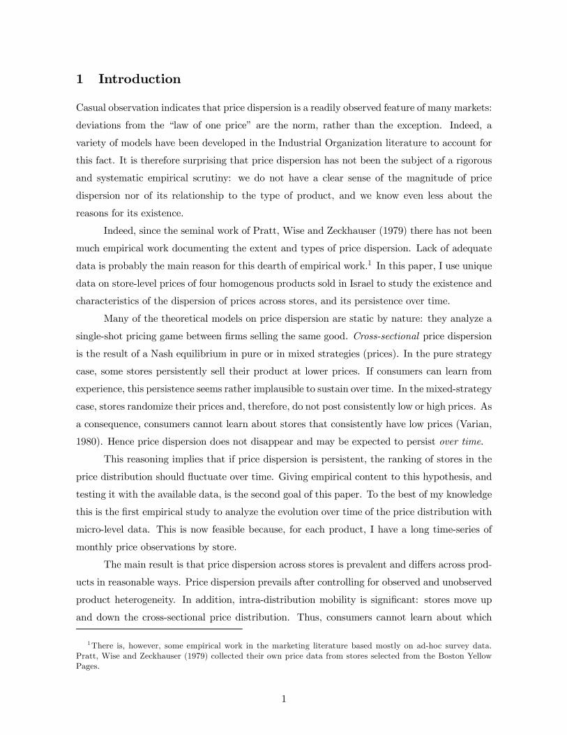
As indicated by the median duration (last row), (at least) 50 percent of the spells in a

given quartile last no more than one month for coffee and chicken (except q4 in the latter),

and at most 2-3 months for flour and for the refrigerator. This means that there is a lot of

“jumping” around the cross-sectional distribution, particularly for coffee and chicken.17

5.3 Transitions between Positions

If duration in a given quartile is short then there is a high probability that, say, next month

the price will jump to a different quartile of the distribution. The transition process from

one cross-sectional distribution (Ft) to another (Ft+1) can be modelled by assuming that this

transition is done in a Markovian fashion through a 4 × 4 transition matrix Tt where its ijthentry gives the probability that a store in the ith quartile in month t (i.e., with a residual

price between qti−1 and qti) moves to the jth quartile in month t + 1. Consistent estimates

of Tt are the sample proportions of stores moving from one quartile to another. Assuming a

time-invariant transition matrix, the 47 estimated transition matrices—one for each transition

between months t and t+1—can be averaged to produce a single (estimated) transition matrix

T.18

Examination of T gives a good idea on the extent of intra-distribution mobility. If stores

keep their positions over time—lack of mobility—then T should have “large” diagonal entries.

If there is a lot of intra-distribution dynamics—mobility—this would be reflected in “large” off-

diagonal probabilities.

The results are presented in Table 6 when the time-horizon is one month (i.e., a transition

between month t and month t + 1). The probability of remaining in the same first quartile

is higher for stores selling the refrigerator (0.78) and flour (0.71) than for the stores selling

chicken (0.51) or coffee (0.43). This result accords with the duration results in Table 5.19 In

fact, the smaller diagonal terms in the food product transition matrices imply that the latter

two products have higher probabilities of moving up and down the price distribution than

17 I recomputed the quartiles and associated duration statistics in Figure 4 and Table 5 using the observedprice of the store—instead of its residual price—and found qualitatively similar features: stores still change theirpositions in the cross-sectional distribution but do so somewhat less often.

18The Markovian and homogeneity assumptions correspond to Quah’s (1993) insight originally developed toanalyze the transition and convergence of country incomes over time. The matrix T is the weighted average ofthe estimated transition probabilities for each month with weights equal to the proportion of observations ineach cell.

19The probability of jumping to another quartile conditional on being in a given quartile (row) is the sum ofthe off-diagonal probabilities in a given row. The (unconditional) probability of jumping is the average of theconditional probabilities which equals the probability of observing a one-month spell.

11

stores selling the refrigerator or flour. Note that mobility is weaker at the extremes of the price

distribution reflecting, perhaps, some (time-varying) unobserved heterogeneity across stores

not captured by (1).

Extending the time-horizon to from 1 to 6 months (i.e., a transition from January to July

to January, etc.) increases intra-distribution mobility (Table 7). As expected, the probability of

remaining within the same quartile after 6 months is quantitatively lower than the probability

of the same event after 1 month. Roughly speaking, these estimates imply that a consumer

that knows the position (quartile) of each store during month t will have approximately a 30-35

percent probability—the average of the estimated diagonal terms—of observing the store in the

same position (quartile) during month t+ 6.20

The estimated transition probabilities are based on a series of strong assumptions re-

garding the order of the Markov process, the time-horizon, the choice of cutoff points in the

distribution, etc.21 Nevertheless, it is comforting that the conclusions reached here are consis-

tent with the duration results in the previous subsection.

5.4 Rank Correlations

A more basic feeling for the persistence in the stores rank can be obtained from the correlations

between stores’ ranks in the residual price distribution across two different months. Figure 6

plots the correlations between the stores’ ranks in January 1993 and their ranks in all subsequent

months (this is just one possible choice out of the 47 possibilities). As expected, the correlations

between the first and subsequent months t is positive for almost all months within the year,

and then oscillate around zero—sometimes considerably. Yet after the first 4-6 months these

correlations are not statistically different from zero.22 This means that knowledge of a store’s

position in any given month is useful in predicting its position in the price distribution up to

no more than 4 to 6 months ahead.

20As Column # indicates many observations are lost when moving from Table 6 to Table 7 because only storeswith consecutive data are included. The literature offers many indices of the degree of intra-distribution mobilitybut, given the small dimension of the transition matrix and the controversy regarding the interpretation of someof the indices, I prefer to present the whole transition matrix here (see Geweke et al., 1986).

21One could in principle generate the 6-month transition from the 1 month-transition matrix. However, it iswell known that there may be inconsistencies across T matrices estimated over shorter and longer time-horizons.This is the case here as well.

22To assess the statistical significance of these estimates we compare them to the exact critical values for thenull hypothesis of no rank correlation. These critical values, tabulated in Table Q of Siegel and Castellan (1988),depend on the number of stores involved in the calculation of the correlation. Using the average number of storesfrom Table 1, the critical values at a 5 percent significance level for the estimated rank correlation are 0.32 forthe refrigerator, 0.33 for chicken, 0.56 for coffee, and 0.54 for flour.

12

In sum, the stability of the cross-sectional price distribution over time masks significant

intra-distribution dynamics. Consumers cannot learn in a definite way which store is charging

what price because the ranking of stores in the distribution changes over time. According to

one measure, a consumer that knows the position of each store during a given month will have

approximately a 30-35 percent probability of observing the same position six months ahead.

According to another measure, after approximately 4-6 months there is no correlation between

the initial rank and the current one. This “short memory” feature of the markets—a reflection of

the significant turbulence in the evolution of the cross-sectional price distribution—is consistent

with a model of consumer search and stores’ use of mixed price strategies (sales). As argued by

Varian (1980), this would preclude rational searchers from identifying the lowest-priced store

over time.

6 Conclusions

This paper measured and analyzed the price dispersion of four homogeneous goods across stores

in Israel over a period of 48 months (1993-1996). The main finding is that price dispersion pre-

vails after controlling for observed and unobserved product heterogeneity. The cross-sectional

price distribution is quite stable over time, but this stability masks an intensive process of stores’

repositioning within the cross-sectional distribution; there is substantial intra-distribution mo-

bility. This finding is consistent with Varian’s (1980) argument about the need for “sales”

(randomized prices) when consumers search rationally for the lowest price.

Is the existence of price dispersion a reflection of strategic behavior or is it driven by

stores’ heterogeneity? As previously observed, price dispersion prevails even after controlling

for product heterogeneity. Thus, heterogeneity cannot be the only reason for the observed

dispersion. Of course, it may still be unobserved (and uncontrolled for) heterogeneity that is

driving this result. But time-invariant heterogeneity has been controlled for, and even if it were

not, this type of heterogeneity cannot generate the observed intra-distribution dynamics. In

principle, time-varying heterogeneity can account for both cross-sectional price dispersion and

intra-distribution dynamics. For example, prices may respond to the arrival of store-specific

(idiosyncratic) shocks, a component of the ε0its in (1). The problem with this interpretation is

that we would need a lot of idiosyncratic “large” shocks arriving every month to destroy the

intertemporal rank correlation. It is difficult to believe that this is happening at the level of

the individual store. Thus, again, heterogeneity alone cannot be the whole story. Indeed, while

it is tempting to interpret the evidence of intra-distribution mobility as reflecting some form

of strategic interaction this is not entirely warranted by the paper’s results. In order to say

13

something about this, additional empirical research is required.

14

References

[1] Burdett, K. and K. L. Judd (1983), “Equilibrium Price Dispersion”, Econometrica, 51,

955-969.

[2] Butters, G. R. (1977), “Equilibrium Distributions of Sales and Advertising Prices”, Review

of Economic Studies, 44, 465-491.

[3] Chamberlin, E. (1933), The Theory of Monopolistic Competition, Cambridge, Mass.: Har-

vard University Press.

[4] Diamond, P. (1971), “A Model of Price Adjustment”, Journal of Economic Theory, 3,

156-168.

[5] Gatti, J. Rupert (2000), “Equilibrium Price Dispersion with Sequential Search”, mimeo,

Trinity College, Cambridge, UK.

[6] Geweke, J., R.C. Marshall and G.A. Zarkin (1986), “Mobility Indices in Continuous Time

Markov Chains”, Econometrica, 54, 1407-23.

[7] Hotelling, H. (1929), “Stability in Competition”, Economic Journal, 39, 41-57.

[8] Lach, Saul and D. Tsiddon (1992), “The Behavior of Prices and Inflation: An Empirical

Analysis of Dissagregated Price Data”, Journal of Political Economy, April, 100(2), pp.

349-389.

[9] Lach, Saul and D. Tsiddon (1996),“Staggering and Synchronization in Price-Setting: Evi-

dence from Multiproduct Firms”, American Economic Review, December, 86(5), pp. 1175-

1196.

[10] Lal, Rajiv and Carmen Matutes (1989), “Price Competition in Multimarket Duopolies”,

Rand Journal of Economics, 20, pp. 516-37.

[11] McAfee, R. Preston (1995), “Multiproduct Equilibrium Price Dispersion”, Journal of Eco-

nomic Theory, 67, 83-105.

[12] McMillan, J. and P.B. Morgan (1988), “Price Dispersion, Price Flexibility and Repeated

Purchasing”, Canadian Journal of Economics, 21, 883-902.

[13] Pratt, J.W., Wise, D. and R. Zeckhauser (1979), “Price Differences in Almost Competitive

Markets”, Quarterly Journal of Economics, 93, 189-211.

15

[14] Quah, D. (1993), ”Empirical Cross-Section Dynamics in Economic Growth”, European

Economic Review, 37, 426-34.

[15] Reinganum, J. (1979), “A Simple Model of equilibrium Price Dispersion”, Journal of

Political Economy, 87, 851-858.

[16] Rob, R. (1985) “Equilibrium Price Distributions”, Review of Economics Studies, 52, 487-

504.

[17] Rothschild, M. (1974), “Searching for the Lowest Price when the Distribution of Prices is

Unknown”, Journal of Political Economy, 82, 689-711.

[18] Siegel, Sidney and N. John Castellan, Jr. (1988), Nonparametric Statistics for the Behav-

ioral Sciences, McGraw-Hill Book Company, international edition, 2nd edition.

[19] Varian, H. (1980) “A Model of Sales”, American Economic Review, 70, 651-659.

16

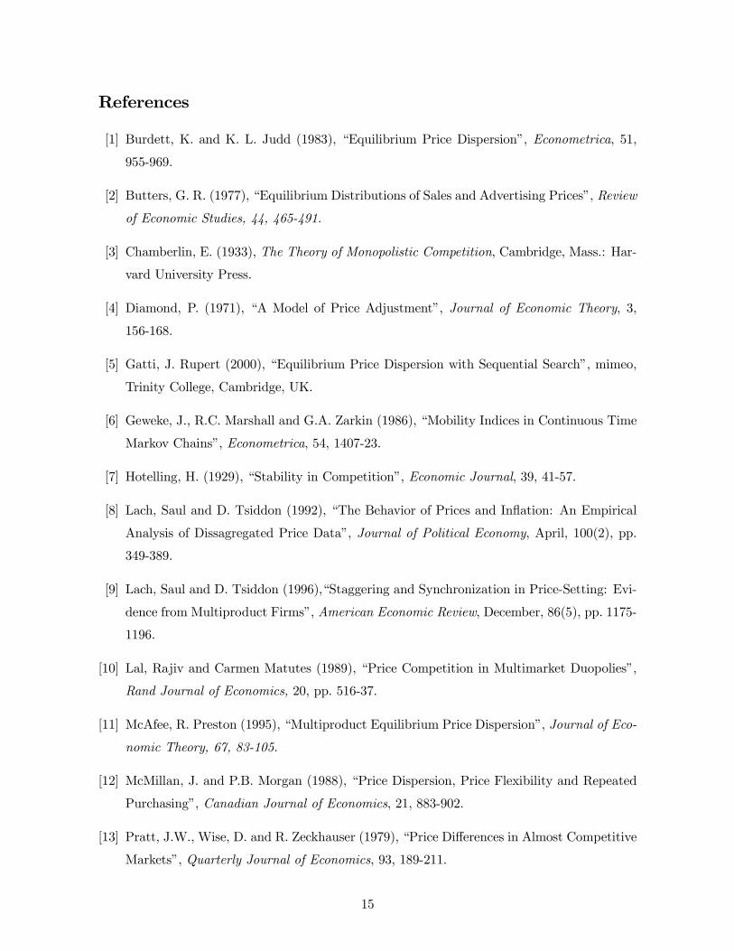
Table 1:List of ProductsProduct No. of Stores Months in Sample No. of Observations

Mean (Min, Max) Mean (Std)

Refrigerator 38.0 (35, 43) 38.0 (14.1) 1826Chicken 36.5 (33, 42) 39.8 (13.3) 1751Size 1 25.1 (22, 29) 40.1 (12.7) 1203Size 2 10.4 (9, 12) 38.5 (14.9) 500

Coffee 13.5 (12, 15) 40.6 (12.6) 649Flour 14.6 (13, 16) 36.9 (13.0) 701

Table 2: Simple StatisticsProduct Mean Price Coefficient of 75% quantile

25% quantile95% quantile5% quantile

2nd highest2nd lowest

(Std) Variation (×100)

Refrigerator 3170.1 (153.9) 4.85 1.05 1.15 1.43Chicken 9.78 (1.13) 11.55 1.17 1.44 2.06Size 1 9.69 (1.10) 11.39 1.15 1.45 2.03Size 2 9.92 (1.18) 11.89 1.18 1.46 1.83

Coffee 11.85 (2.33) 19.66 1.51 1.79 2.30Flour 1.55 (0.21) 13.35 1.19 1.41 2.00Prices not in logs and deflated to January 1993. Estimates are on the pooled data,i.e., over months and stores.The number of observations appears in Table 1.

Table 3: Tests for Group Effectsp-value of F-test

Refrigerator Chicken Coffee Flour

Month Effects 1.00 0.00 0.00 0.00Store Effects 0.00 0.00 0.07 0.00City Effects 0.00 0.00 0.00 0.00Type Effects — 0.00 0.12 0.21Size Effects — 0.00 — —

N 1826 1751 649 641∗

R2 0.50 0.60 0.91 0.83

R2

0.47 0.57 0.90 0.81Based on OLS estimates of equation (1). Storesselling the refrigerator are all of the same type.∗The flour equation is 60 observations short from the numberin Table 1 because two stores have missing type data.

17

Table 4: Price Dispersion MeasuresMonthly Averages

Product Standard Quartiles Differences in QuantilesDeviation 25% 75% 75%-25% 95%-5%

Refrigerator 0.0323 -0.0171 0.0143 0.0313 0.1048Chicken 0.0728 -0.0408 0.0458 0.0865 0.2361Coffee 0.0585 -0.0232 0.0306 0.0538 0.2205Flour 0.0436 -0.0232 0.0247 0.0479 0.1600Price dispersion based on bεit.Averages over 48 months of the plots in Figures 3.

Table 5: Distribution of Durations by Quartile(percentages)

Duration

1 month2 months3 months4 months5 months6+ months

MeanMedian

Refrigeratorq1 q2 q3 q4

27.2 33.3 30.1 25.221.1 21.4 22.7 20.98.8 14.9 18.4 11.310.5 15.5 11.0 13.09.7 6.6 9.8 4.422.7 8.4 8.0 25.2

4.02 2.70 2.77 4.033 2 2 3

Chickenq1 q2 q3 q4

57.2 61.2 60.9 45.122.5 21.7 24.8 19.68.6 9.7 10.2 13.04.1 4.7 1.5 10.31.4 0.8 1.5 6.06.2 1.9 1.1 6.0

1.99 1.69 1.61 2.421 1 1 2

Duration

1 month2 months3 months4 months5 months6+ months

MeanMedian

Coffeeq1 q2 q3 q4

66.3 66.7 61.9 55.820.0 25.7 21.6 20.97.4 1.9 9.3 8.11.1 2.9 4.1 9.31.1 1.9 3.1 2.34.1 0.9 0.0 3.6

1.71 1.52 1.65 1.941 1 1 1

Flourq1 q2 q3 q4

36.7 45.1 38.6 40.08.2 19.7 27.1 14.018.4 16.9 17.1 16.014.3 9.9 7.1 8.010.2 2.8 4.3 4.012.2 5.6 5.8 18.0

3.20 2.28 2.30 3.223 2 2 2

18

Table 6: One-Step Transition Matrix (1-month horizon)

Refrigerator# q25 q50 q75 ∞

439 q25 0.78 0.11 0.07 0.04439 q50 0.18 0.65 0.09 0.08440 q75 0.02 0.22 0.65 0.11447 ∞ 0.03 0.02 0.17 0.78

Chicken# q25 q50 q75 ∞

429 q25 0.51 0.20 0.18 0.11423 q50 0.26 0.42 0.23 0.09418 q75 0.13 0.27 0.39 0.21431 ∞ 0.10 0.10 0.19 0.61

Coffee# q25 q50 q75 ∞

155 q25 0.43 0.21 0.13 0.23155 q50 0.23 0.35 0.30 0.12154 q75 0.10 0.32 0.41 0.17164 ∞ 0.23 0.11 0.17 0.49

Flour# q25 q50 q75 ∞

152 q25 0.71 0.10 0.09 0.10158 q50 0.20 0.58 0.11 0.11155 q75 0.06 0.27 0.59 0.08157 ∞ 0.02 0.06 0.21 0.71

Based on residual prices bε. Column # gives the number of price quotations in the initialquartile which equals the sum over months of the number of stores in each quartile.A store enters the calulations only when it has data on two consecutive periods. Entriesare weighted averages of the month-specific probabilities of moving from one quartileto another with weights given by the proportion in each month of the total observationsin the intial quartile (Column #)

19

Table 7: One-Step Transition Matrix (6-month horizon)

Refrigerator# q25 q50 q75 ∞

64 q25 0.38 0.25 0.17 0.2060 q50 0.32 0.25 0.16 0.2763 q75 0.14 0.32 0.33 0.2168 ∞ 0.18 0.18 0.29 0.35

Chicken# q25 q50 q75 ∞

65 q25 0.31 0.34 0.24 0.1158 q50 0.28 0.28 0.27 0.1760 q75 0.23 0.23 0.22 0.3264 ∞ 0.20 0.13 0.23 0.44

Coffee# q25 q50 q75 ∞

23 q25 0.26 0.26 0.17 0.3121 q50 0.38 0.24 0.24 0.1420 q75 0.25 0.30 0.30 0.1525 ∞ 0.20 0.08 0.28 0.44

Flour# q25 q50 q75 ∞

21 q25 0.24 0.33 0.19 0.2423 q50 0.26 0.26 0.31 0.1723 q75 0.31 0.17 0.35 0.1731 ∞ 0.13 0.16 0.13 0.58

See notes to Table 6.

20

ln (real price), deviation from monthly average

Chicken

0

.01

.02

.03

.04

Coffee

Flour

-.5 -.25 0 .25 .5

0

.01

.02

.03

.04

Refrigerator

-.5 -.25 0 .25 .5

Figure 1: Price Densities

21

Refrigerat

-0.08

-0.06

-0.04

-0.02

0

0.02

0.04

0.06

0.08

0.1

1 3 5 7 9 11 13 15 17 19 21 23 25 27 29 31 33 35 37 39 41 43 45 47

month

Q10 Q25 Q50 Q75 Q90

Chicken

-0.15

-0.1

-0.05

0

0.05

0.1

0.15

1 3 5 7 9 11 13 15 17 19 21 23 25 27 29 31 33 35 37 39 41 43 45 47

month

Q10 Q25 Q50 Q75 Q90

Coffee

-0.25

-0.2

-0.15

-0.1

-0.05

0

0.05

0.1

0.15

1 3 5 7 9 11 13 15 17 19 21 23 25 27 29 31 33 35 37 39 41 43 45 47

month

Q10 Q25 Q50 Q75 Q90

Flour

-0.15

-0.1

-0.05

0

0.05

0.1

0.15

1 3 5 7 9 11 13 15 17 19 21 23 25 27 29 31 33 35 37 39 41 43 45 47

month

Q10 Q25 Q50 Q75 Q90

Figure 2: Quantiles of the Residual Price Distribution

22

epsilon

Chicken

0

.05

.1

.15

Coffee

0

.05

.1

.15

Flour

-.5 -.25 0 .25 .5

0

.05

.1

.15

Refrigerator

-.5 -.25 0 .25 .5

0

.05

.1

.15

Figure 3: Cross-sectional Residual Price Densities

23

Refrigerator

.25

.5

.75

q1pcnt q2pcnt q3pcnt

12

34

56

78

910

1112

1314

1516

1718

1920

2122

2324

2526

2728

2930

3132

3334

3536

3738

3940

4142

4344

4546

4748

Chicken

.25

.5

.75

q1pcnt q2pcnt q3pcnt

12

34

56

78

910

1112

1314

1516

1718

1920

2122

2324

2526

2728

2930

3132

3334

3536

3738

3940

4142

4344

Coffee

.25

.5

.75

q1pcnt q2pcnt q3pcnt

12

34

56

78

910

1112

1314

1516

Flour

.25

.5

.75

q1pcnt q2pcnt q3pcnt

12

34

56

78

910

1112

1314

1516

17

Figure 4: Time Spent in each Cross-sectional Quartile (%)

24

Std

RefrigeratorStore

1 5 10 15 20 25 30 35 40 45 50

1

5

10

15

20

Std

ChickenStore

1 5 10 15 20 25 30 35 40 45

1

5

10

15

20S

td

FlourStore

1 5 10 15 20

1

3

6

Std

CoffeeStore

1 5 10 15 20

1

3

6

Figure 5: Standard Deviation of Stores’s Ranks

25

Sp

ea

rma

n (

1,t

)

month

Chicken

-1

-.5

0

.5

1

Coffee

-1

-.5

0

.5

1

Flour

1 6 12 24 36 42 48

-1

-.5

0

.5

1

Refrigerator

1 6 12 24 36 42 48

-1

-.5

0

.5

1

Figure 6: Rank Correlations (1,t)

26