NBER WORKING PAPER SERIES

EVIDENCE ON GROWTh,INCREASING RETURNS AND THE

EXTENT OF THE MARKET

Alberto F. AdesEdward L. Glaeser

Working Paper No. 4714

NATIONAL BUREAU OF ECONOMIC RESEARCH1050 Massachusetts Avenue

Cambridge, MA 02138April 1994

We are grateful to Robert Barro, José Scheinkman. Andrei Shleifer and participants at theHarvard Growth Seminar for very helpful comments. Matt Botein and Melissa McSherryprovided excellent research assistance. We acknowledge financial support from the NationalScience Foundation and the Toner/Clark Fund. This paper is pait of NEER's researchprogram in Growth. Any opinions expressed are those of the authors and notthose of theNational Bureau of Economic Research.

NBER Working Papa #4714April 1994

EVIDENCE ON GROWTh,INCREASING REI1JRNS AND THE

EXTENT OF THE MARKET

ABSTRACT

We examine two sets of economies (19th century U.S. states and 20th century less

developed countries) where growth rates axe positively correlated with initial levels of

development to document how these dynamic increasing returns operate. We find that open

economies do not display a positive connection between initial levels and later growth; instead,

closed economies do display this positive correlation (i.e. divergence). This evidence suggests

that increasing returns operate by expanding the extent of the market (as in the big push theories

of Murphy, Shleifer and Vishny (1989)). For U.S. states, we also find that larger markets

enhance growth by increasing the division of labor. Among LDCs, while more diversified

production increases growth, diversification is negatively associated with openness for the poorest

economies (as in the quality ladder theories of Boldrin and Scheinkman (1988). Young (1991)

and Stokey (1991)). However, and despite the negative effect that openness has on the diversity

of production and, thus, on growth, we find that openness still substantially increases growth for

these poorer economies.

Alberto F. Ades Edward L. GlaeserDepartment of Economics Department of EconomicsHarvard University Harvard UniversityCambridge, MA 02138 Cambridge, MA 02138

and NBER

1. Introduction

Following Allyn Young (1928), much of the recent theoreticalwork on economic growth builds on

increasing returns to scale in production. Unlike models based on neoclassical production functions, these

models suggest that steady-state per capita growth rates arenot independent of initial conditions.' Romer

(1983 and 1986), Lucas (1988), Murphy. Shleifer and Vishny (1989), Rebelo (1991) and others use

increasing returns so that initial levels are positivelycorrelated with later growth rates and the endogenous

portion of growth continues indefinitely. Under particular assumptions, these models suggest that the the

world's lead economy will display divergence over time and often they also predict that the cross-section

of the world's economies will also not show convergence.

But empirical work on cross-country growth generally finds convergence, not divergence. Baumol

(1986), DeLong (1988), Barro (1991), Barro and Sala-i-Martin (1992) and Mankiw, Rozner and Weil

(1992) document patterns of convergence in cross-country and U.S. data. Across countries, per capita

GDI's do not converge unconditionally between 1960 and 1985,but they do converge once we condition

on variables (such as education) that determine the steady state level of income per capita. This evidence

would seem to contradict modern endogenous growth theory.'

In fact, the well-documented conditional convergence of Barro and Sala-I-Martin (1992) and others is

more relevant for tests based on the neoclassical growth model. Endogenous growth models predict

unconditional, not conditional, divergence.' Most of these theories also predict that increasing returns

should operate only during specific time periods (i.e. during industrialization) or 'in specific countries.

We use the term neoclassical to refer to production functions that display diminishing returns toscale.

'Growth theorists (see, for example, Romer (1986)) tend to avoid this contradiction by emphasizingthat divergence need only appear in the time series evidence of the lead economy. In many models

divergence is not predicted in a cross section.

'Technically, the issue is whether or not savings or schooling behavior should be treated as an

exogenous variable (as Solow (1957) treats Investment), or whether they should be considered asendogenously determined by other initial conditions. Barro (1991) takes a partial approach, treatingschooling as only a right hand side variable but treating investment as endogenouslydetermined by other

initial conditions.

Instead of testing implications of the neoclassical growth model against the alternative hypothesis of

endogenous growth, we proceed by testing the hypotheses of endogenous growth models against each

other and against the alternative hypothesis that increasing returns never operate.

Our primary question is whether increasing returns occur because higher Initial GD)' acts to increase

the demand for national products. Recent papers such as Becker and Murphy (1993) or Murphy, Shleifer

and Vishny (1989) predict that growth %Ilows initial wealth because that wealth creates a market for

certain activities. According to these models, higher initial income should increase later growth rates

more strongly when an economy is closed than when an economy isopen. In open economies, aggregate

demand is fixed by world markets and higher initial levels of income do not change effective demand.

In closed economies, national income determines demand.

We address this question with two samples of economies that display wacondllionaldynamic increasing

returns (U.S. states in the 19th century and the 65 poorest countries in 1960).' In our country sample

we use income and urbanization to measure growth and the share of trade in GD)' to measure openness.

Across U.S. states, we use the state's levels of urbanization (following De Long and Shleifer (1993)) and

manufacturing to measure development. Nineteenth century income data for U.S. states is neither reliable

(despite heroic efforts by Easterlin and others) nor theoretically appropriate in economies with

considerable amounts of migration between states. For the states, we use physical distance to major

regional ports (and, thus, to major east coast markets)' and regional railroad development as our basic

measures of openness.'

Across all of our samples, we find that increasing returns axe important for closed no:open economies.

This evidence suggests that increasing returns operate by expanding the extent of the market as in big

'The importance of these samples immediately tells us about that there are places where increasingreturns do operate.

'Such physical measures could also be used for 20th century data for U.S. states or cross-countrycomparisons. However, the vastly improved nature of transportation makes reliance on geography muchless palatable in the age of the airplane, truck and high speed ocean transport. See Pred (1980) for amore detailed discussion of these issues.

'Regional rail has the useful attribute of giving us time series as well as cross-sectional variation.

2

push theories (Rosenstein-Rodan (1943) and Murphy, Shlelfer and Vishny (1989)) or theories where

growth derives from the division of labor (Becker and Murphy (1993)). This finding does not support

the implication of quaiity ladder arguments that openness is particularly damaging for economies at the

very bottom of the income distribution (see Stokey (1991) or Young (199!)).

We explore ftzrther the relationship between initial levels, openness and growTh with a variety of

decompositions. For both the nineteenth century U.S. data and the world data, the division of labor spurs

growth. In the U.S. data, initial GD? and openness increase growth in part by increasing the division

of labor. For world data, initial GDP raises the division of labor, but openness deters it (as in Stokey

(1991)). However, while openness acts against growth in poorer countries by reducing the division of

labor, the overall connection between openness and growth for the poorest nations is strongly positive -

- the direct positive effects of openness overwhelm the indirect effect that works through lost diversity.

Section Il discusses the relevant theories. Section III describes the data. Section IV presents our basic

empirical results starting with the openness/increasing returns connection. The next two sections present

our decompositions. Section VII concludes.

II. Theories of Increasing Returns

This section presents the relevant implications of four major sets of theories of endogenous growth.

lnformatiortoi Access

In Romer (1983, 1986), endogenous growth is obtained with an aggregate production functioo that

exhibits increasing returns that are eiternal to the investing finn. Knowledge-based growth theories may

predict that openness spurs growth because of the connection of trade to information transmission (e.g.

reverse engineering of traded goods, the Italian merchant Marco Polo, the Portuguese traders in 16th

3

century Japan, or the innovations brought by European traders to native Americans).' But even if

openness increases access to a wider set of ideas for all countries,it is not obvious bow it interacts with

growth at different levels of development. Two effects seem likely to drive the cross-effect between

openness and initial GD?: (1) bigher human capitalcould make it easier to take advantage of new ideas

so more developed areas may benefit most from the exposure created by trade, and (2) the new ideas

brought by trade might be less new to more developed countries. Evidence on the openness-initial GDP

cross-effect can help determine the relative importance of these two effects but it cannot be used as a test

for the roleof informational spillovers more broadly.

Big Pushes

A second theory of increasing returns is the big push theory of Rosenstein-Rodan (1943) and Murphy,

Shleifer and Vishny (1989). This theory emphasizes the importance of coordination and demand

spillovers in generating increasing returns and multiple equilibria. Technically, the Murphy a a!. models

also rely on the existence of fixed costs (and hence increasing returns) in technology, but the emphasis

of their work lies on the role that increasing levels of income play in creating a larger market for

industrialized output.

According to the theory of the big push, within closed economies more initial wealth creates more

demand for industrialized products which in turn induces firms to pay the fixed costs of growth. By

contrast, in small open economies the demand curves facing local producers are set by world markets and

uninfluenced by local wealth.' The big push theory predicts that growth will be related to initial wealth

and access to world markets but also that the interaction between wealth and openness will be negative

'Of course, some European innovations, such as the Inquisition, may not have been good for growth.

'This type of effect might be part of the explanation for the smooth post-war Japanese business cycle.This emphasis on pecuniary externalities links growth with Keynesian (1936) macroeconomics. A naturaltest of the importance of pecuniary externalities for business cycles is to compare output volatility(relative to world output) for open and closed economies.

4

as openness eliminates the linkage between initial wealth and effective demand. We also test for the

importance of the big push by checking if the extent of the market works by increasing the rate of growth

of physical capital (where fixed costs are most likely to matter).

Diversity and Specializaüon

A third set of increasing returns theories with implications for openness emphasize the role of

specialization. The connection between the division of labor and economic progress is typically

associated with Smith (1976). Becker and Murphy (1993) argue for the role that the division of labor

plays in increasing both the level and the growth rate of income over time.' A finer division of labor

can speed up growth because concentration in a single task might facilitate innovation and learning by

doing (as Smith suggested). The costs of acquiring new skills might also lower as the range of tasks

involved diminishes.'0

Smith's famous dictum is that the division of labor is limited by the extent of the market. If that is

true, growth should be connected to initial levels only in closed economies. In open economies, the

world market is what determines the extent of the market. These models predict the same negative

interaction between openness and initial wealth as the big push theories, but they also predict that the

positive effect of the extent of the market on later growth should lessen when we control for the division

of labor.

'Becker and Murphy emphasize the importance of coordination as opposed to actual market size for

the division of labor. However, their model also allows for the standard Smithian effects ofmarket size.

These effects becomeparticularly close in spirit to their work whenthe statistical returns to scale of largermarkets are taken into account, i.e. when larger markets work by diversifying Idiosyncratic demand

shocks to particular consumers.

'° A supposed advantage of assembly lines is the ease of training assembly line employees.

S

The Qualisy Ladder: SpecialWng in the Wrong Products

A final set of theories that offer predictions on the relationship between increasing returns and openness

are the quality ladder arguments of Boldrin and Scbeinbnan (1988), Stokey (1991), Grossman and

Heipman (1991) and Young (1991), and the 19th century protectionists List (1856) and Rae (1834).

Quaiity ladder theories are tied to the division of labor theories in that they argue that the range of goods

produced is critical to growth, but in the quality ladder theories openness lessens diversity in production.

Divisionof labor theories emphasize the importanceoftbehigberdemand forabroader rangeof products

that comes about with increased openness; quality ladder models emphasize bow openness raises the

foreign supply of these products, and thus lessens the effective demand for the domestic production of

those products.

Under quality ladder arguments, openness is particularly damaging for the extremely poor countries.

With free trade, less developed countries will tend to specialize in low growth activities that are intensive

in the use of natural resources or unskilled labor, thereby allowing middle income countries to reallocate

their resources away from these low growth activities)' In Stokey's words "if the industries in which

the less developed country has a static comparative advantage are industries in which there are limited

opportunities for learning, then the effect of free trade is to speed up learning in the more developed

country and to slow it down in the less developed one." Therefore, and contrary to big push and division

of labor theories, quality ladder arguments predict that initial income will be more closely associated with

later growth for open economies than for closed economies.

III.- The Data

This section describes our data sets and their construction.

"High income countries may in fact also reduce growth as they reduce their production of high

growth products and cater more to world tastes.

6

Construction oft/ic Data Sets

our cross-counuy data set was constructed using several different sources. The data on urbanization

were assembled by hand from bard copy, and come from the 1988 edition of the Frospeas of World

llrbwdzationi' The cross-countzy data on population and real per capita GD? are from the Barro and

Wolf (1991) data set. The trade data are from theWorld Bank's World Tables, and consists on imports

and exports of goods and non-factor services. Data on educational attainment is from Barro and Lee

(1993). The data on road infrastructure is from Canning and Fay (1992), and the land area data come

from the 1986 edition of the FAQ Production Yearbook

For the U.S. states, we also used a variety of different sources. The data on state population.

urbanization and labor force are from the Historical Statistics oft/ic United States (1976). For population

in the state's main city, we used the 1980 Census and several issues of the Statistical Abstract oft/ic

United Stases. For some states, we used direct 19th century census data. The data on the labor force

engaged in manufacturing in 1880 and 1890 is from several issues of Statistical Abstract of the United

States. For earlier years, we used the 1840 to 1870 censuses."

The railroad data for 1860 to 1890, and the data on distance from the state's main city to the main

regional city are from the Ssatisticoi Abstract oft/ic United Stases. For each port, the relevant regional

port was either New York, San Francisco or New Orleans, whichever was closer. The railroad data for

1840 and 1850 is from Wicker (1960). Literacy data are taken from the U.S. censuses. We had no

12 Data are available only for countries or areas with two million or more inhabitants in 1985.

"A problem with the U.S. census labor force and manufacturing data is that the populatioà covereddid not remain invariant during our sample period. Thus, while the 1840 and 1870 censuses covered thewhole population, the 1850 census covered the free male labor force above 15 years of age only, and the1860 census included free females and extended the age limit to 10 years or older. We dealt with thisproblem by obtaining census estimates of the slave population. To. construct labor shares inmanufacturing, we assumed that all slaves of 15 years of age and older were In the labor force, and that15 percent of them were in manufacturing (we based this figure on Sokoloff (1982)). Before thesecorrections, Southern states displayed wild variations in their manufacturing shares. We also tried alteringour assumptions about slave labor force participation rates and shares In nianufactur'mg slightly but noneof our results seemed sensitive to these alterations.

7

choice but using data on white literacy only as before 1860 the census provides no Information on literacy

rates for the slave population. Finally, we gathered data on over 300 hundred occupations from the 1850

and 1810 censuses.

Our U.S. data thus covers the deódes 1840-1890. Data was not collected before 1840 because of

availabilityproblems. We stopped in 1890 because (1) massive immigration to eastern cities potentially

biases our results, (2) rail development had become extremely comprehensive by 1890 so variation across

regions became less meaningfol, and (3) by 1890 the eastern states had achieved a similar level of

development to the most developed nations in ourcross-country sample. Moreover the period 1840-1890

is typically considered the era of America's big push?

Descripilon of the Data

Tables Ia and lb show the five fastest and five slowest growers in our cross-country sample ftioth in

tenns of GD? and urbanization) and the corresponding initial levels of the relevant variable. While the

average initial income of the fastest growers is about $ 150 (in 1980 dollars) higher than that of the

slowest growers, the group shows considerable heterogeneity. It includes both relatively well-off countries

as Malta and extremely poor ones as Lesotho. This is not the case with the slowest growers; all of them

are in Sub-Saharan Africa.

In terms of urbanization, the distinctions are more clear-cut. The average level of initial urbanization

for the fastest growers is about double that of the slowest ones. Korea is the fastest grower on both

counts,' and only five of the twenty countries are outside Sub-Sabaran Africa. Table Ic shows the five

most and five least urbanized U.S. states in 1840, and table Id does the same thing for 1890.. Table le

shows the largest and smallest spurts in urbanization growth. Table If shows the largest and smallest

changes in urbanization over the 1840-1890 sample.

" There is a strong correlation between urbanization and Incomegrowth across countries. Webelieve this fact supports our use of urbanization in the U.S. regressions.

8

IV. Evidence on Increasing Returns and the Extent of the Market

There are two major ways in which our estimation differs from more standard forms, e.g. Barro

(1991): (1) we often use urbanization not income as our measure of development, (2) we focus on

unconditional not conditional regressions.

Urbanization vs. Income

Our emphasis on urbanization (and manufacturing) over income for U.S. state data goes against the

prevailing methodology and, admittedly, urbanization is often a poor proxy for economic development."

However, the standard data source on state income levels (Easterlin (1960 used by Barro and Sala-i-

Martin (1992)) is available oniy at 40 year intervals, has measurement problems, and is in nominal dollar;

(so differences across states might not reflect local price level differences). On the contrary,

urbanization is (1) available every 10 years, (2) a simple, reliable measure, (3) invariant with respect to

local price indices, and (4) reliably connected with economic development (see Bairoch (1988)).

We also favor urbanization over income in the 19th century U.S. because intrastate mobility should

eliminate any welfare differences across states. The income differences that do exist should represent a

combination of unobserved heterogeneity and compensating differentials. The high incomes earned in

19th century western states are much better interpreted as a compensation for the danger of the frontier

and tediousness of life away from the eastern seaboard than as an index of economic development. Table

la shows the five least urbanized states of the U.S. in 1840. Without exception these states represent

some of the least developed areas of the United Sta;es in this period.

U The exact model that we have in mind is spelled out in the estimating framework section of the

paper.

9

Condirionoi vs. (Jnconditionoi C.onwrgence

We first focus on unconditional convergence rather than on the more traditional examination of

conditional convergence. This focus is appropriate since the four theories described above concern

unconditional increasing returns. An advantage of the unconditional regressions Is that they are less prone

to measurement error blase. When regressing GDP growth on initial GDP, measurement error creates

both the standard bias, which lowers the absolute value of the coefficient on initial GDP,1' but when

measurement error is i.i.d., it also lowers the coefficient on initial GDP by

Var(Measuremen, Error) (I)Var(JnifloJ GD?)

When conditional regressions are run, this second bias becomes

Var(Measzjremem Error) (2)Vor(lnifial GD? onhQgonollzed with respect to the other controls)

Since the denominator in (6) might be substantially smaller than that in (5), the bias towards convergence

might be much higher in conditional regressions. In the case of standard growth regressions, the bias

towards convergence more than triples when going from unconditional to conditional regressions."

Estinzo.sing Framework

The appropriate model for using urbanization as a proxy for development is one with two sectors: a

primary, unurbanized, agricultural, or low technology sector, and a secondary, urbanized, or

manufacturing one. Aggregate production in each state is given by

This coefficient is given by

Cov(GDP aonge,Ininai GD!')Var(InizjoJ GD!')

The first bias works by raising the denominator. The second bias operates by lowering the numerator.

"This extra bias may explain why divergence appears in unconditional regressions only.

10

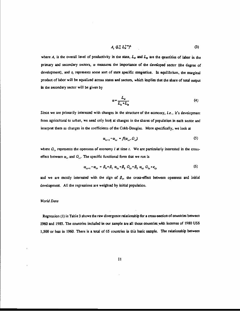
A, (L; L41' (3)

where A, is the overall level of productivity in the state, L,, and L2 are the quantities of labor in the

primary and secondary sectors, a measures the importance of the developed sector (the degree of

development), and s, represents some sort of state specific congestion. In equilibrium, the marginal

product of labor will be equalized across states and sectors, which implies that the share of total output

in the secondary sector will be given by

a- (4)

Since we are primarily interested with changes in the structure of the economy, i.e.. it's development

from agricultural to urban, we need only lool at changes in the shares of population in each sector and

interpret them as changes in the coefficients of the Cobb-Douglas. More specifically, we look at

a41.1ajj —f(a,1,O,) (5)

where C),, represents the openness of economy I at time 1. We are particularly interested in the cross-

effect between a,, and 0,. The specific functional form that we run is

a fi0+$1 cr4,.$2 O,+$ a4, O,+e,,, (6)

and we are mostly interested with the sign of , the cross-effect between openness and initial

development. All the regressions are weighted by initial population.

World Data

Regression (I) in Table 3 shows the raw divergence relationship for a cross-section of countries between

1960 and 1985. The countries included in our sample are all those countrieswith Incomes of 1980 USS

1,500 or less in 1960. There is a total of 65 countries in this basic sample. The relationship between

11

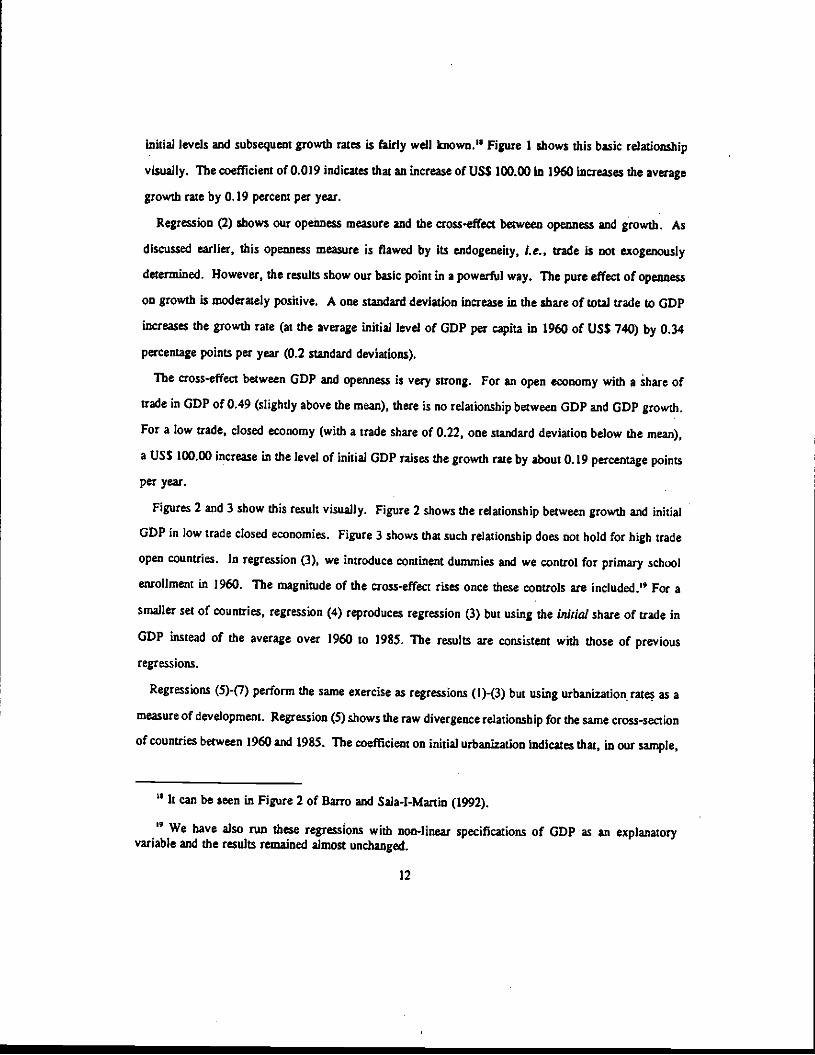
initial levels and subsequent growth rates is fairly well known." Figure 1 shows this basic relationship

visually. The coefficient of 0.019 indicates that an increase of USS 100.00 in 1960 increases the average

growth rate by 0.19 percent per year.

Regression (2) shows our openness measure and the cross-effect between openness and growth. As

discussed earlier, this openness measure is flawed by Its endogeneity, I.e., trade is not exogenously

determined. However, the results show our basic point in a powerilil way. The pure effect of openness

on growth is moderatelypositive. A one standard deviation increase in the share of total trade to GD?

increases the growth rate (at the average initial level of GD? per capita in 1960 of USS 740) by 0.34

percentage points per year (0.2 standard deviations).

The cross-effect between GDP and openness is very strong. For an open economy with a share of

trade in GD? of 0.49 (slightly above the mean), there is no relationship between GDP and GD? growth.

For a low trade, closed economy (with a trade share of 0.22, one standard deviation below the mean),

a USS 100.00 increase in the level of initial GD? raises the growth rate by about 0.19 percentage points

per year.

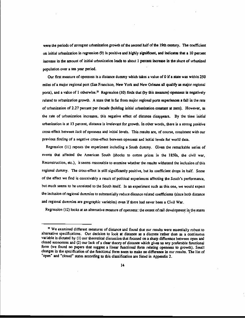
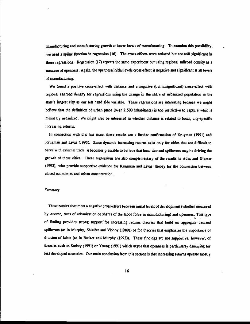
Figures 2 and 3 show this result visually. Figure 2 shows the relationship between growth and initial

GDP in low trade closed economies. Figure 3 shows that such relationship does not hold for hightrade

open countries. In regression (3), we introduce continent dummies and we control for primary school

enrollment in 1960. The magnitude of the cross-effect rises once these controls are included." For a

smaller set of countries, regression (4) reproduces regression (3) but using the initial share of trade in

GD? instead of the average over 1960 to 1985. The results are consistent with those of previous

regressions.

Regressions (S)-(7) perform the same exercise as regressions (1X3) but using urbanization rates as a

measure of development. Regression (5) shows the raw divergence relationship for the same cross-section

of countries between 1960 and 1985. The coefficient on initial urbanization indicates that, in our sample,

"It can be seen in Figure 2 of Barro and Sala-I-Martin (1992).

"We have also run these regressions with non-linear specifications of GD? as an explanatoryvariable and the results remained almost unchanged.

12

a :10 percent increase in the initial level of this variable is associated with 4 percentage points faster

increase in urbanization over the period.

Regression (6) shows that once again the cross-effect is negative and strong. For, a moderately open

economy with a share of trade in (DP of 0.46 (3 percentage points above the mean), there is no

relationship between initial urbanization and subsequent changes. For a relatively closed economy (with

a trade share of 0.22, one standard deviation below the mean), a 10 percent increase in the level of initial

urbanization leads to a 4 percent increase in urbanization over the period.

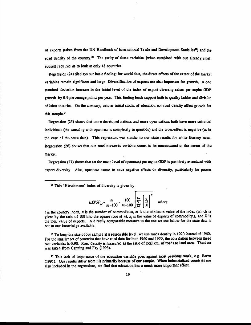
Figure 4 displays this strong positive relationship for the closed economies in our 65 least developed

countries. Figure 5 shows that there is no relationship between changes and initial levels for the open

economies. Again, regression (7) verifies that our results are robust to controlling for regional and

educational variables. Regression (8) shows that our results are not sensitive to using the share of trade

from 1960 to 1985 as our measure of openness.

U.S. Data

Table 4 contains similar regressions for our U.S. states sample. This table shows results for a pooled

sample of states over the period 1840-1890. The decade 1860-1870 has been eliminated due to the Civil

War?' We have included fixed effects for each decade and allowed for correlation across decades in

the shocks to states by estimating a stacked set of growth regressions with SUR techniques (state specific

random effects are a particular form of this methodology with an assumed form of correlation across

decades). The SUR methodology ensures that a state's growth rate between 1870 and 1880 aid a state's

growth rate between 1880 and 1890 are not treated as independent observations.'

Our dependent variable is the decadal change in the share of urbanized population in the state. The

first regression in Table 4 documents the basic positive relationship between urbanization growth and

initial levels of urbanization. The time dummies tell us that the 1840-1850 and the 1880-1890 decades

r The results become substantially stronger if that decade is included.

31 In fact there is not that mucb correlation between decadal growth rates across states.

13

were the periods of strongest urbanization growth of the second half of the 19th century. The coefficient

on initial urbanization in regression (9) Is positive and highly significant, and indicates thata 10 percent

increase in the amount of initial urbanization leads to about I percent increase in the share of urbanized

population over a ten year period.

Our first measure of openness is a distance dummy which takes a value of 0 if a state was within 250

miles of a major regional port (San Francisco, New York and New Orleans all qualify a major regional

ports), and a value of I otherwise. Regression (10) finds that (by this measure) openness is negatively

related to urbanization growth. A state that is far from major regional ports experiences a fall in the rate

of urbanization of 2.27 percent per decade fliolding initial urbanization constant at zero). However, a

the rate of urbanization increases, this negative effect of distance disappears. By the time initial

urbanization is at 13 percent, distance is irrelevant for growth. In other words, there is a strong positive

cross-effect between Jack ofopenness and initial levels. This results are, of course, consistent with our

previous finding of a negative cross-effect between openness and initial levels for world data.

Regression (11) repeats the experiment including a South dummy. Given the remarkable series of

events that affected the American South (shocks to cotton prices in the 1850s, the civil war,

Reconstruction, etc.), it seems reasonable to examine whether the results withstand the inclusion of this

regional dummy. The cross-effect is still significantly positive, but its coefficient drops in half. Some

of the effect we find is conceivably a result of political experiences affecting the South's performance,

but much seems to be unrelated to the South itself. In an experiment such as this one, we would expect

the inclusion of regional dummies to substantially reduce distance related coefficients (since both distance

and regional dummies are geographic variables) even if there had never been a Civil War.

Regression (12) looks at an alternative measure of openness: the extent of rail development iothestates

n We examined different measures of distance and found that our results were essentially robust toalternative specifications. Our decision to look at distance as a discrete rather than as a continuousvariable is dictated by (I) our theoretical discussion that focused on a sharp difference between open andclosed economies and (2) our lack of a clear theory of distance which gives us any preferable functionalform (we found no papers that suggest a linear functional krm relating openness to growth). Smallchanges in the specification of the functional form seem to make no difference In our results. The list ofopen' and closed states according to this classification are listed in Appendix 2.

14

that belong to the same census region as the state, with the exclusion of the state in question? States

surrounded by neighbors with highly developed transportation systems constituted larger potential markets

for the state in question. In addition, they facilitated access from the main production sites in the state

to major regional ports. These arguments justify using regional rail development as a proxy for state

openness. Here again we see a very powerfial negative cross-effect between openness and growth. Initial

urbanization only matters for states in regions with poorly developed railroad networks.

Regression (13) allows the relationship between changes and initial levels to be non-linear. We use

a spline function with breaks at relatively arbitrary points (urbanization rates of 50 percent is the break

between high and low urbanization). The positive coefficient on initial urbanization is higher for low

urbaiiization rates. Both state and world data indicate this type of concavity. Even more interesting is

that the coefficient on initial urbanization is even stronger once we look at the interaction between low

urbanization and distance. The coefficient increases by 50 percent. There is no cross-effect between

urbanization and distance for high urbanization states because all of the states with more than 50 percent

urbanization rates are situated close to a major port. Regression (14) looks at an unbalanced panel. This

avoids our random effects-style methodology (that requires a balanced panel) and simply pools all the

available data together. The cross-effect between distance and initial urbanization is highest for this

regression?

Table S shows results for changes in the share of the labor force employed in manufacturing and

changes in the share of urbanized population living in the state's largest city. The manufacturing

regressions only cover the 1870-90 decades as we do not have reliable manufacturing data for the earlier

periods. Unlike urbanization. manufacturing shares mean revert for states that are near major ports, but

display divergence for closed economy states.

Since manufacturing seems to display strong decreasing returns at higher levels, we worried that some

of the distance/initial share connection might only be capturing the stronger positive connection between

There are 9 census regions: Pacific, Mountain, West North Central, East North Central, MiddleAtlantic, New England, South Atlantic, East South Central, and West South Central.

However, interpreting the standard errors Is not simple as we incorrectly treat state urbanizationchanges as independent over tUne.

IS

manufacturing and manufacturing growth at lower levels of manufacturing. To examine this possibility,

we used a spline function in regression (16). The cross-effects were reduced but are still significant in

these regressions. Regression (17) repeats the same experiment but using regional railroad density as a

measure of openness. Again, the openness/initial levels cross-effect is negative and significant at all levels

of manufacturing.

We found a positive cross-effect with distance and a negative ut insignificant) cross-effect with

regional railroad density for regressions using the change in the share of urbanized population in the

state's largest city as our left hand side variable. These regressions are interesting because we might

believe that the definition of urban place (over 2,500 inhabitants) is too restrictive to capture what is

meant by urbanized. We might also be interested in whether distance is related to local, city-specific

increasing returns.

In connection with this last issue, these results are a further confirmation of Xrugman (1991) and

Krugman and Livas (1993). Since dynamic increasing returns exist only for cities that are difficult to

serve with external trade, it becomes plausible to believe that local demand spillovers may be driving the

growth of these cities. These regressions are also complementary of the results in Ades and Glaeser

(1993), who provide supportive evidence for Krugrnan and Livas' theory for the connection between

closed economies and urban concentration.

Summary

These results document a negative cross-effect between initial levels of development (whether measured

by income, rates of urbanization or shares of the labor force in manufacturing) and openness. This type

of finding provides strong suppor( for increasing returns theories that build on aggregate demand

spillovers (as in Murphy, Shleifer and Vishny (1989)) or for theories that emphasize the importance of

division of labor (as in Becker and Murphy (1993)). These findings are not supportive, however, of

theories such as Stokey (1991) or Young (1991) which argue that openness is particularly damaging fOr

less developed countries. Our main conclusion from this section is that increasing returns operate mostly

16

for less developed economies by expanding the size of the market.

V. The Division of labor, Human Capital and Infrastructure.

In the previous section, we focused on the interaction between level of development and openness as

a means of distinguishing between theories of increasing returns, Le., these three variables tried to

establish that initial growth spurred subsequent growth by increasing the extent of the market. We will

subsequently refer to our three previous variables (initial levels, openness and the interaction) as extent

of the market variables. Here, we are interested in testing further between the basic theories by including

othervariables related to initial conditions: (I) diversity of production, (2) human capital, and (3) physical

infrastructure. Following Murphy, Shleifer and Vishny (1992), we examine whether the extent of the

market variables remain significant when controlling for these variables and we decompose the effect of

the basic variables into direct effects and indirect effects going through the new variables.

The main variable that will help distinguish among the three theories is the diversity of production

variable. Both quality ladder and division of labor theories predict a strong effect of the range of

products on growth. In quality ladder models, more products suggest more high growth products; in

division of labor theories, more products and occupations suggest more division of labor. But while in

quality ladder arguments openness reduces the variety of products, in division of labor models openness

increases the range of products. We will also be looking at thepossibility that human capital or physical

infrastructure are behind the connection of growth with the extent of the market.

Esrfrrtathig Framework

The estimating framework simply uses equation (4). Instead of assuming that growth is a function of

openness and initial levels only, we assume that growth is related to initial levels, openness and other

variables that were previously omitted. However, these new variables might also be correlated with

openness and initial levels. We can then decompose our previous egisnates of the effects of openness,

Il

initial levels and the cross-effect into the direct effects and the indirect effects operating through our

previously omitted variables. More precsdy, we assume that

a,J.I—aL, '.f(Z(a,11O1j.a,,,OJ (7)

where Z is the vector of variables that were omitted from (4). The particular functional form that we

estimate is

$0+ôZ(cr,,O)e$1 a,,+P, a,, 0ç, (8)

where e,4 is a noise term. We also assume that

(9)

The total effect of initial levels on further growth can therefore be decomposed into a direct effect of $,

and an indirect effect operating through Z of fry,. Similarly, the total effect of openness on growth is

given by a direct effect of $2 and an indirect effect of fry,. Finally, the interaction can be decomposed

into a direct effect of fi, and an indirect effect of fry,. These effects add Up to the coefficients estimated

in (4).

These decompositions have the interpretation of asking how much initial levels or openness work

directly on growth and how much their effects work indirectly by raising the levels of other variables that

are correlated with growth. We can then ask, for example, how much of the cross-effect between

openness and growth works directly and how much it affects growth by allowing a thinner division of

labor among tasks. We consider three possible sources of increasing returns: (I) human capital spillovers

(meant to be related to the knowledge stories outlined above), (2) physical infrastructure, and (3) the

division of labor.

World Data

Table 6a shows the regressions used for the decompositions that we do with world data. The variables

in the Zvector are the share of the population with complete secondary schooling, a measure of diversity

18

of exports (taken from the UN Handbook of International Trade and Development Statistics') and the

road density of the country. The rarity of these variables (when combined with our already small

subset) required us to look at only 43 countries.

Regression (24) displaysour basic finding: for world data, the direct effects of the extent of the market

variables remain significant and large. Diversification of exports are also important for growth. A one

standard deviation increase In the initial level of the index of export diversity raises per capita GD?

growth by 0.9 percentage points per year. This finding lends support both to quality ladder and division

of labor theories. On the contrary, neither initial stocks of education nor road density affect growth for

this sample?

Regression (25) shows that more developed nations and more open nations both have more schooled

individuals (the causality with openness is completely in question) and the cross-effect is negative (as in

the case of the state data). This regression was similar to our state results for white literacy rates.

Regression (26). shows that our road networks variable seems to be unconnected to the extent of the

market.

Regression (27) shows that (at the mean level of openness) per capita GD? is positively associated with

export diversity. Also, openness seems to have negative effects on diversity, particularly for poorer

' This "Hirschmann' index of diversity is given by

3

EZPSPithlOOl00oQj [II is the country index, n is the number of commodities, m is the minimum value of the index (which isgiven by the ratio of 100 into the square root of ii), x is the value of exports of commodityj. and X isthe total value of exports. A directly comparable measure to the one we use below for the state data isnot to our knowledge available.

To keep the size of our sample at a reasonable level, we use roads density in 1970 instead of 1960.For the smaller set of countries that have road data for both 1960 and 1970, the correlation between thesetwo variables is 0.98. Road density is measured as the ratio of total km. of roads to land area. The datawas taken from Canning and Fay (1993).

' This lack of importance of the education variable goes against most previous work, e.g. Barro(1991). Our results differ from his primarily because of our sample. When industrialized countries arealso included in the regressions, we find that education has a much more important effect.

19

countries. As in Boldrin and Scheinkinan (1988) or Stokey (1991), openness reduces the range of

products sold. As we found in regression (24), this reduction of diversity in turn reduces growth. Here,

the supply effect of openness (i.e. outside suppliers reduce product range) must be dominating the demand

side effect (larger markets allow a larger product range). Finally, the cross-effect between openness and

growth is positive, which suggests that trade increases diversity for more developed countries. We take

these results as providing some support for quality ladder stories. While there is a negative effect of

openness on diversification for poorer countries, the overall effect of openness on growth for these poorer

countries is strongly positive. The direct effect of openness on growth for these nations overwhelms the

much smaller indirect effect of openness on growth that operates through specialization of production.

U.S. Data

Data availability limits our decades to 1850-1860 and 1870-1880. Again, we look at changes in the

degree of urbanization as a function of initial urbanization, our distance dummy and the cross-effect

between the two. We are interested both in the decomposition of initial levels and in the cross-effect

between urbanization and distance.

Our human capital variable is the white literacy rate of the state in 1850 and 1870. Our measure of

physical infrastructure is railroad density of the state in question. Our measure of specialization is a

tixit-Stiglitz" variety index created by using occupational data hand collected from the 1850 and 1870

censuses. The specific functional form that we use for this last variable is given by

DS, ,- enwlo.inzenI., (10)

aggregate eraploynlenJ,,

where i is the state, and) is the occupation.

This measure of specialization might be somewhat sensitive to the definitions used in each census to

define each category of employment. Because these definitions changed over census years, we resealed

the indices of specialization obtained by subtracting from the corresponding value for each state-decade

20

the decadal sample mean and dividing by the decadai standard deviation. Thus, our measure of

specialization keeps the same mean and standard deviation over both periods. This specialization measure

is ideal for capturing the division of labor — it strongly weights the presence of obscure professions. It

seems much less ideal for measuring quality ladder effects, but it should also be related to the range of

products being produced in a state.

Regression (24) in Table 7a shows the results of running changes in the share of urbanized population

on time fixed effects, the extent of the market variables, physical infrastructure (measured by railroads

in the state), white literacy levels and our measure of division of labor. In these regressions, the direct

effects of the extent of the market disappear statistically. Human capital does predict later growth but

only weakly. Railroads and the division of labor are both extremely strong predictors of later itate

growth. A one standard deviation increase in the Dixit-Stiglitz diversification measure raises the change

in the share of urbanized population by about 2.5 percentage points.

Regressions (25) and (27) show that both initial levels of urbanization and the cross-effect are

correlated with higher levels of literacy and specialization. This last regression strongly supports the

basic Smithian notion that the division of labor is limited by the extent of the market and it is through

this division of labor that growth occurs. Regression (26) shows that while local railroad density is not

related to the cross-effect, it is extremely strongly correlated with initial urbanization. The stock of

physical infrastructure (which is strongly related to later growth) thus seems to be connected to initial

levels of development, but not merely to the extent of the market. While these regressions certainly leave

room for big push theories, they most strongly suggest that growth in U.S. states was associated with the

division of labor and that this division of labor was only possible in states with either a high degree of

initial development or access to ports.

The MI decomposition is performed in Table 7b. The positive effect of initial urbanization occurs

mainly through initial specialization and local railroads density. The negative effect of distance works

mainly through lower specialization, and somewhat less through lower human capital. In this sample.

openness increases the degree of diversification of products, contrary to the predictions of quality ladder

stories. The positive cross-effect mainly operates through increased specialization and higher levels of

21

human capital. These high human capital people then act to further growth directly through their work

and by generating knowledge spilovers.U

The difference between these results and those In the world sample may come from the difference in

the proxy used kr specialization. In the U.S. data, the diversification measure was accurately picking

up the presence of highly specialized occupations. In the world data, the measure is more closely linked

to the degree of specialization in a few export products and it does not necessarily capture the internal

division of labor within the country? The overall conclusion of this section Is that In both samples the

division of labor sped later growth. However the samples disagree about what creates the divison of

labor. In the U.S. sample, urbanization and openness both increased the degree'of division of labor and

the cross effect between those two variables lowered the division of labor; basic Smithian notions about

the division of labor being limited by the extent of the market are strongly supported. In the world

sample. In the world sample, the arguments of quality ladder theorists are supported. The division o(

labor rises with openness only for the richer counties. Poorer countries produces a smaller range of

products when they are exposed to larger markets.

VI. Decomposing Growth In Physical Capital, Human Capital and Technology

This subsection decomposes GD? growth into, the growth of physical capital, human capital and

technology. We are not interested here in whether or not the extentof the marketvariables work through

increasing initial levels of specialization or initial levels of human capital. Instead, we want to know

whether the extent of the market raises growth through (1) accumulation of physical capital, (2)

accumulation of human capital, or (3) technological progress. We are decomposing growth into these

three different forces not through the traditional growth accounting methods but, rather, using a

decomposition borrowed from the labor literature. We begin by ascertaining the effect of levels of

The large empirical literature relating initial human capital levels and growth across U.S. areasincludes Glaeser, Scheinkman and Shleifer (1993), Simon and Nardinelli (1993) and others.

29 In fact, this specialization of exports in a single good may lead towards a better division of laborwithin the country.

22

physical and human capital on levels of production with a cross-sectional levels rçgression. Then we use

those coefficients to decompose growth into human and physical capital accumulation and growth of the

residual (which is similar to the basic Solow residual)? We then examine bow the extent of the market

variables affect the growth of physical and human capital.

Estimating Framework

We assume that the level of urbanization or income in economy tat time t is given by

a0cA, F(114.K,,) (ii)

and we specifically assume the following functional form for our regressions

a11=A,+62 H,1+52 +J# (12)

where H, and IC, measure human and physical capital in economy I at time:, and v is the error term in

the regression." The underlying assumption is that the level of development is restricted by the

availability of physical and human capital, and by the overall level of technology.

116, and 6. are time invariant, we can decompose the changes in urbanization or per capita income into

a,,,,1 —a1, t4,, —A, .6, '..H,,) +6, (c,,.1 —K,)• p1,.1 — (13)

The first term in this decomposition is constant across countries orstates of the U.S. and drops out in

the regressions. The second and third terms reflect those changes in urbanization or income that are

explained by human and physical capital accumulation. The final term reflects 'the residual change.

We then regress these individual components on our standard initial variables and examine through

which channels these initial variables affect later growth. Specifically, we regress

r This type of decomposition is similar to Glaeser (1993).

'tWe assume a linear specification in the logs of physical and human capital as In a standard Cobb-Douglas technology. We do not, however, constrain the coefficients to add to one since we are notassuming that we have accurately captured all of the factors of production.

23

•1-Fi-)4+)4 a,,+)4 O,,+)4 a,, O,,.4 (14)

,1-x,,,->4.>4 a,,+)4 o,,.i4 a 05)

and

—v-)4.X a,,,+>4 0> a,,, O,,+C (16)

We can then decompose the effects of initial urbanization or GDP, openness and the interaction into

their different components. Thus, the total effect of initial development, openness and the interaction

between the two are given, respectively, by

o x.o, x+x; (17)

6 )4+63 x.x; (18)

and

s, x,o2 x+x; (19)

The intuition for these decompositions is simple. We are dividing the effect of initiai development,

openness and their interaction into their effects operating through human capital accumulation, physical

capital accumulation, and changes in productivity.

For the purposes of this section, we combine initial development, openness and the cross-effect into

a single extent of the markeC variable. This variable is formed by taking a weighted average of these

three sub-variables. The weights come from running the basic growth regressions (i.e. regressions (I)

and (7)) for the sub-sample under examination. This combination is meant to simplify the intition.

World Darn

For our cross-country sample, we used actual capital stock estimates from Canning and fly (1992) as

our measure of physical capital. Human capital is measured by the share of the population over 25 years

24

of age with complete primary schooling (from Barro and Lee (1993). Table Ba shows that levels of GD?

are much more associated with physical capital than with the stock of human capital. The decomposition

shown in Table Sb reveals that the extent of the market worked much more through physical than through

human capital. The results from this decomposition thus lend support to big push ideas: the importance

of larger markets lies in creating the conditions for physical capital investment rather than in providing

the incentives for Investing In human capital. However, the growth of the residual is by far the most

important channel through which the extent of the market affects growTh: almost 80 percent of the extent

of the market operates through this last channel. This finding suggests that the main effect of larger

markets is to allow for improvements in the level of technology.

U.S. Data

In Table 9a, regression (32) shows that both white literacy and railroad density (our measures of human

and physical capital) are positively correlated with levels of urbanization. A one percent increase in the

white literacy rate raises the level of urbanization by 1.3 percent. A one standard deviation increase in

railroad density within the state increases the share of urbanized population by 12 percent. Regressions

(33X35) are the auxiliary regressions that we use for our decomposition. This decomposition is shown

in Table 9b. We find that the effect of the extent of the market on technolOgical change explains about

less than a fifth of the total. Human capital is instead not associated with larger initial market size.

Finally, we find that most of the effect of the extent of the market operates through the accumulation of

physical infrastructure. In other words, large market size increased growth by spurring physical

investment in railroads. These results lend support again to big push arguments, which the

importance of investments with large fixed costs to explain increasing returns.'2

In the

We should remind the reader that there might be something particular about this form of investmentthat relates to urbanization. Since urbanization specifically measures a form of population concentration,and railroad development specifically measures the development of transportation, an alternativeinterpretation of this result is that the concentration of population leads to transportation improvements.

25

VII. Conclusion

This paper presents a variety of evidence on the connection between initial levels of development and

later growth. We found that a positive connection between levels and later growth is muck stronger in,

closed rather than open economies. This evidence provides support to the notions that the size of the

market matters for growth because of access to global ideas, because a larger market allows for

investment in large fixed cost investments and because the division of labor is limited by the extent of

the market. The evidence does not support quality ladder type of theories, or other protectionist theories

that suggest that isolation from world markets is particularly good for poor economies.

We found in a set of decompositions that diversity in occupations (for U.S. states) or exports (for

countries) both enhanced growth. Openness and market size increased occupational diversity in the U.S.

and much of the effect of the extent of the market on growth seems to work through bigger markets

creating a finer division of labor. Openness and market-size did not increase diversity of exports. Just

as in Stokey (1991) or Young (1991), openness decreased the range of products for many countries.

However, we still found that cur openness variabks speeded growth for poorer countries despite the costs

associated with losing export diversity. Our last set of decompositions suggested that the extent of the

market may work through the division 01' labor, but it seems to enhance growth mainly by speeding

investment in physical infrastructure. We found our two sets of evidence supporting both division of

labor theories and theories emphasizing the role of market size in allowing for big physical investment.

This work does cast doubt on the protectionist suggestions of quality ladder theories. While our

results do support. their idea that protectionism allows a broader range of products to be produced, our

results also suggest that protectionism has other problems which overwhelm this product range effect.

Our work cannot determine how exactly protectionism detracts from growth for poorer countries.

Potential explanations include (1) growth requires markets or (2) isolation exacerbates political problems

or (3) closedness means separation from international pools of technology, but future work will be needed

to determine which mechanism is actually in effect.

26

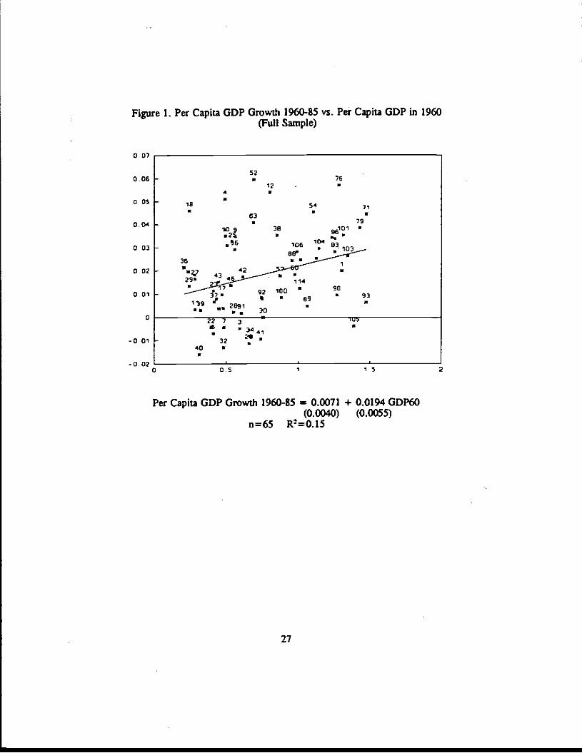
Figure 1. Per Capita GDP Growth 1960-85 vs. Per Capita GDP in 1960

0.07

(Full Sample)

0.05

O 05

0.04

o 03 -

0.02 -

0.01

0

-0 01

-0.021 15 2

Per Capita GDP Growth 1960-85 = 0.0071(0.0040)

n65 R2=0.15

27

+ 0.0194 GDP6O(0.0055)

18

40

.2_36a

5276

12 . —

S

54 71S

630 79

38 95101S

35S

—V29S

106880a

421S

S

100a

•0

90S 93

a

p114a

9269

2891 5•5 55 30

227 3 -'U,a

3240 a

S

0

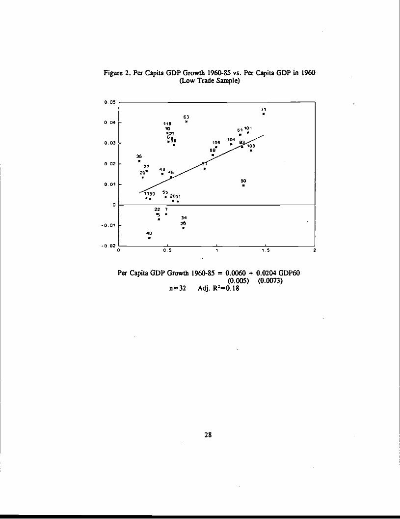
Figure 2. Per Capita GDP Growth 1960-85 vs. Per Capita GDP in 1960(Low Trade Sample)

0 . 05

71

630.0.4 - 118

25

• 103003-

3688

29 45

0 02

0 01 .1139 55

• 28s1

022 7

— 34-0.01 -

40w

-0.02 I0 0.5 1 1.5 2

Per Capita GDP GroMh 1960-85 = 0.0060 + 0.0204 GDP6O(0.005) (0.0073)

n32 Adj. R20.18

28

Figure 3. Per Capita GDP Growth 1960-85 vs. Per Capita GD? in 1960(High Trade Sample)

0.07

520.06 - 7612 I

40.05 -

18 54I0.0-4 -

9 36 96I • I0.03

24 51I0 . 02

2370.01 92 100I I.

300

3 IUDII41

.001 - 32 II

—0.02 I0 0.5 1 1.5 2

Per Capita GDP Growth 1960-85 = 0.0228 + 0.0052 GDP6O(0.0107) (0.012)

n=33 Mj.R2=-0.0258

29

Figure 4. Change in

0.3 —

0.25

0.2

o is

01.

0.05 -

Urbanization 1960-85 vs. Urbanization in 1960

(Low Trade Sample)

0 01 0.2 03 0.4 05 06

Change in Urbanization 1960-85 = 0.0303 + 0385 Urbanization 1960(0.017) (0.0761)

35

6 101S

BB

7 103S

29S

104.5

83S

S40S

20 9127 3t

61K

2P5*

5.7K

43S

115539w

F

56S

106 rnK

90.S

0

n32 R2OM

30

Figure 5. Change in Urbanization 1960-85 vs. Urbanization in 1960(High Trade Sample)

0452

S

23 41S S

033

.216

0292

31 32 — 76

60 105w

00 01 02 03 04 0.5 0.6 07 0.8

Change in Urbanization 1960-85 = 0.135 - 0.179 Urbanization 1960(0.055) (0.208)

n=33 Adj. R=-O.0081

31

Table IaDescription of the Data

State Annual Per Capita GD? Per Capita GD? iGrowth 1960-1985

n 1960

Korea

Five Fastest Growers

6.0 690

Malta 5.7 3280

Gabon 5.4 804

Benin 5.1 595

Lesotho

Zaire

4.6 245

Five Slowest Growers

-1.6 314

Somalia -1.3 483

Madagascar -1.1 659

Zambia -0.9 740

Sudan -0.8 667

TABLE lbDescription of the Data

Staie Change in Percentage of PercentageUrbanized Population Urbanization in

1960-19851960

Korea

Five Fastest Growers

38 28

Mauritania 32 5

Zambia 4! 17

Cameroon 29 14

Brazil

Sri Lanka

28 45 .

Five Slowest Growers

3 18

Guyana 3 29

Burundi 3 2

Rwanda 4 2

Uganda 4 5

32

TABLE IcDescription o( the Data

State Total Population Percentage Urban

Rhode Island

Five Most Urbanized U.S. States In 1840

109,000 44

Massachusetts 738,000 38

Louisiana 352,000 30

Maryland 470,000 24

New York

Arkansas

2,429,000 19

Five Least Urbanized U.S. States in 1840

98,000 0

Florida 54,000 0

Iowa 43,000 0

Vermont 292,000 0

Wisconsin 31,000 0

TABLE IdDescription of the Data

State Total Population Percentage Urban

Rhode Island

Five Most Urbanized U.S. States in 1890

346,000 85

Massachusetts 2,239,000 82

New York 6,003,000 65

New Jersey 1,445,000 62

Connecticut

Mississippi

746,000 50

Five Least Urbanized U.S. States in 1890

1,290,000 5

Arkansas 1.128,000 6

North Carolina 1,618,000 7

Alabama 1,513,000 10

South Carolina 1,151.000 10

33

TABLE I.Description of the Data

State Change in Percentage Decade

New Jersey

Five Largest Decathi Increasesin the Percentage of Urbanized Population

15 1850-1860

Illinois 14 1880-1890

Massachusetts 13 1840-1850

Rhode Island 12 1840-1850

Rhode Island

Louisiana

II 1860-1870

Five Largest Decadal Declinesin the Percentage of Urbanized Population

4 1840-1850

Louisiana 2.5 1870-1880

South Carolina I 1870-1880

Mississippi 0.9 1870-1880

Alabama - 0.9 1870-1880

TABLE IfDescription of the Data

State Cbange in Percentage Urbanization in 1840

New Jersey

Five Largest Changes in thePercentage of Urbanized Population 1840-1890

52 IINew York 46 19

Massachusetts 44 38

Illinois 43 2

Rhode Island

Louisiana

41 44 .

Five Smallest Changes in thePercentage of Urbanized Population 1840-1890

-4 30

Mississippi 4

South Carolina 4 6

North Carolina 5 2

Arkansas 6 10

34

TABLE 2aWorld Summary Statistics

Variable Obs Mean SW. Dev Minimum Maximum

Per Capita GDP in 1960in thousands of 1980 USSat PPP prices(C D P60)

65 0.74 0.37 0.21 1.47

Average Per Capita GD?Growth 1960-85(CR6085)

65 0.018 0.018 -0.016 0.06

Openness(OPEN)

65 0.43 0.22 0.09 1.22

Urbanization in 1960(IJRBAN6O)

65 0.22 0.14 0.018 0.70

Change in the Share ofUrbanized Population1960-85(URCH)

65 0.14 0.078 0.032 0.38

Percentage of TotalPopulation with CompleteSecondary Education in1960(SSCÔO)

54 0.017 0.019 0.0001.

0.018

Capital Stock per Capitain 1960(KAPC6O)

54 1380.5 1067.1 78.10 3937.2

Roads Density in 1970(RDDEN7O)

43 2974 18522 5.48 121600

Export Specialization.Division of Labor(EXPSP)

43 0.48 0.18 0.008 0.844

35

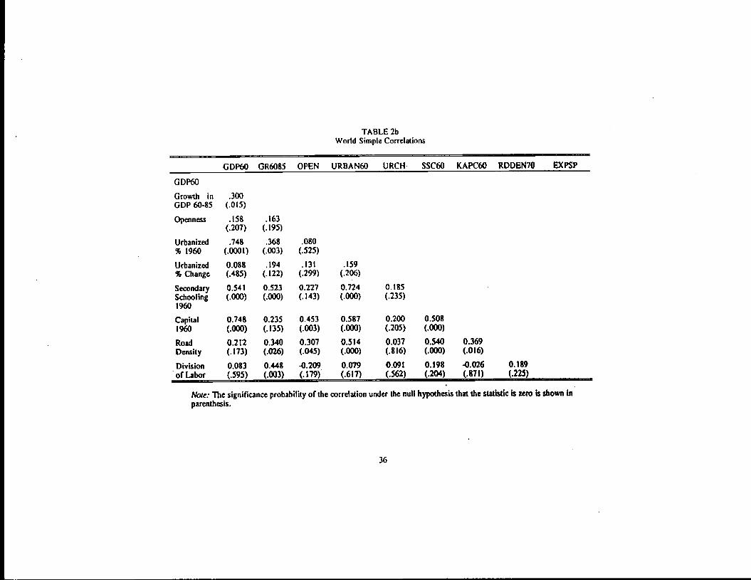
TABLE 26World Simple Correlations

CDP6O CR6085 OPEN URBAN® URCH• SSC6O KAPCS3 RDDEN7O EXPSP

GDP6O

Growth in .300GDP 60-85 (.0 15)

Openness .158 .163(.207) (.195)

Urbanized .748 .368 .080% 1960 (.0001) (.003) (.525)

Urbanized 0.088 .194 .131 .159% Change (.485) (.122) (.299) (.206)

Secondary 0.541 0.523 0.227 0.724 0.185

Schooling (.000) (.000) (.143) (.000) (.235)1960

Capital 0.748 0.235 0.453 0.587 0.200 0.5081960 (.000) (.135) (.003) (.000) (.205) (.000)

Road 0.212 0.340 0.307 0.514 0.037 0,540 0.369

Density (.173) (.026) (.045) (.000) (.816) (.000) (.016)

Division 0.083 0.448 -0.209 0.079 0.091 0.198 -0.026 0.189of Labor (.595) (.003) (.179) (.617) (.562) (.204) (.87 1) (.225)

Note: The significance probability of the correlation under the null hypothesis that the statistic Is zero is shown in

parenthesis.

36

TABLE 2cU.S. Sununazy Statistics

Variable Obs Mean SW. Dev Minimum Maximum

Population in 1870(POP7O)

Urbanization in 1870(UR7O)

change in Share ofUrbanized Population1870-80(1JRCH)

Local Railroads

Density in 1870(RAIL7O)

Regional RailroadsDensity(EXRL7O)

Land Area(LAREA)

Share of UrbanizedPopulation in MainCity in 1870(MCITSH7O)

Change of the Shareof UrbanizedPopulation in MainCity 1870-80(MCITCH)

White Literacy Ratein 1870(WLR7O)

Occupational Dixit-Stiglitz Index for1870(1)570)

Share of the LaborForce inManufacturing(MAN70 )

Change in the Shareof the Labor Force inManufacturing (1870-80)(MANCH)

29 0.23

29 0.033

29 61.85

29 47.60

29 36.43

29 0.1!

29 0.006

29 0.93

29 0

42 0.14

42 -0.007

0.18 0.024

0.035 -0.025

47.90 4.85

30.52 2.50

20.59 1.058

0.10 0.01

0.021 -0.033

0.03 1 0.85

I -1.36

0.13 0.014

0.74

0.1 07

187.20

115.34

69.322

0.34

0.061

0.98

1.84

0.56

0.0623

29 1214 981 12$ 4382

0.030 -0.088

37

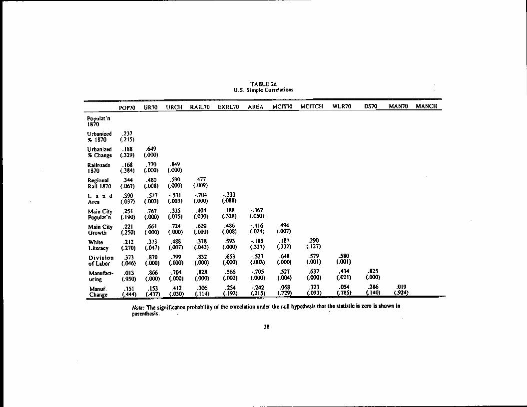
TABLE2dU.S. Simple Correlations

p0P70 UR7O URCI-I RAIL7O EXRL7O AREA MCIT7O MCITCH WLR7O £1570 MAN7O MANCH

Populat'n1870

Urbanized .237% 1870 (.215)

Urbanized .188 .649% Change (.329) (.000)

Railroads .168 .770 .8491870 (.384) (.000) (.000)

Regional .344 .480 .590 .477Rail 1870 (.067) (.008) (.000) (.009)

L a 11 d .390 -.527 -.531 -.704 -.333Area (.037) (.003) (.003) (.000) (.088)

Main City .251 .767 .335 .404 .188 -.367

PopulaCn (.190) (.000) (.075) (.030) (.328) (.050)

Main City .221 .661 .724 .620 .486 -.4 16 .494Growth (.250) (.000) (.000) (.000) (.008) (.024) (.007)

White .212 .373 .488 .318 .593 -.185 .187 .290

Literacy (.270) (.047) (.007) (.043) (.000) (.337) (.332) (.127)

Division .313 .870 .799 .832 .653 -.527 .648 .579 .580of Labor (.046) (.000) (.000) (.000) (.000) (.003) (.000) (.00 I) (.001)

Manufact- .013 .866 .704 .828 .566 -.705 .527 .637 .434 .825

wing (.950) (.000) (.000) (.000) (.002) (.000) (.004) (.000) (.021) (.000)

Manuf. .151 .153 .412 .306 .254 -.242 .068 .323 .054 .286 .019

Change (.444) (.437) (.030) (.114) (.192) (.215) (.729) (.093) (.785) (.140) (.924)

Mire: The significance probability of the correlation under the null hypothesis that the statistic is zero is shown in

parenthesis,

38

TABLE 3

Dependent Variable: Avaage Per Capiia GDP1960-85

Growth Cbae In Urbanlzatio1960-85

n

(I) (2) (3) (4) (5) (6) (7) (8)

Intercept .0071

(.0040)-.0095 -.0191(.0012) (.0061)

-.0101(.0078)

3.767(1.636)

-7.327 -6.713(2.927) (3.611)

.6.037(3.504

Per Capita GDP in1960

.0194(.0055)

.034! .0345

(.0100) (.0096).0280

(.0124)

Openness' .0802 .1404

(.0283) (.0216).0812

(.0270)49.78 32.11

(11.28) (12.71)17.10

(11.47

Per Capita GDP in1960 Openness

-.0703 -.1252(.0357) (.0268)

-.0779(.0289)

.

Urbanization in 1960 .3792

(.0709).7551 .5321

(.1285) (.3828).5603

(.1764

Urbanization in 3960• Openness

-1.641 -1.056(.4785) (.5275)

-.9358(.4412

Primary SchoolEnrollment in 3960

.0139(.0070)

.0146(.0107)

6.195(4.231)

8.034(4.894

Suh-Sabaran Africa

Dummy

.0234(.0037)

-.0231(.0059)

5,658(2.241)

7.869(2.700

Latin American

Dummy

-.0058

(.0053)-.0061(.0068)

3,787(3.225)

2.849

(3.338

NumberofObservations

65 65. 65 56 65 65 65 56

Adjusted R' 0.15 0.25 046 0.45 0.30 0.47 0.51 0.50

Note: Standard errors are in parentheses.'In regressions (4) and (8), Openness Is defined as the share of trade In GD? In 1960.

39

TABL.E 4

Dependent Variable: (9) (10)Decadal Change in theShare of Urbanized

(11) (12) (13) (14)(IJobal)

.

Population (1840-1890)

1840 Fixed Effect .0382 .0419 .0748 .0248 .0457 0.0456(.0059) (.0090) (.0084) (.0063) (.0097) (.0087)

1850 Find Effect .0036 .0450 .0756 .0153 .0418 .0412(.0068) (.0097) (.0093) (.0077) (.0138) (.0085)

1870 Find Effect .010) .0146 .0562 -.0217 .0106 .0076(.0066) (.0102) (.0112) (.0090) (.0112) (.0091)

1880 Fixed Effect .0385 .0406 .0858 .0068 .0390 .0378(.0075) (.1068) (.0122) (.0098) (.0112) (.0093)

Initial Urbanization .0917 .0710 .0020 .1918 .0917(.0198) (.0223) (.0239) (.0317) (.0200)

Distance Dummy -.0227 -.0224 -.0194 -.0224(.0109) (.0090) (.0116) (.0092)

Distance Dummy * Initial .1122 .0870 .2010Urbanization (.0429) (.0042) (.0378)

Initial Regional Railroads .0007Density (.0001)

Initial Regional Railroads -.0020Densitylnitial (.0003)Urbanization

South Dummy -.0413(.0071)

Initial Urbanization * Low .0914Urbanization Dummy (.028 1)

Initial Urbanization • High .0621Urbanization Dummy (.0223)

initial Urbanization • Low .1465Urbanization Dummy • (.0451)Distance Dummy

Initial Urbanization • HighUrbanization DummyDistance Dummy

Number of Observations 116 116 116 116 116 160

Adjusted R2 0.24 0.40 0.61 0.43 0.43 0.82

Note: Standard errors are in parentheses.

40

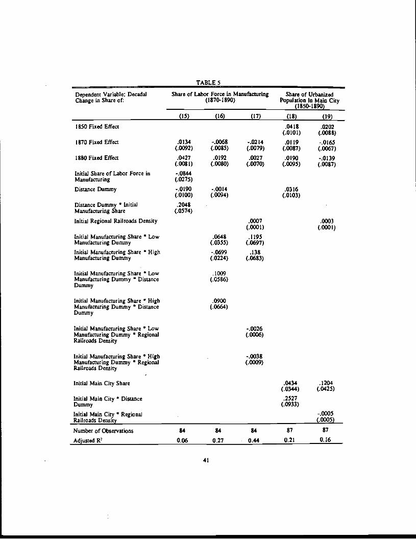
TABLE 5

Dependent Variable: DecadalChange in Share of:

Share of Labor Force in Manufacturing(1870-1890)

Share of UrbanizedPopulation In Main City

(1850-1890)

(IS) (16) (17) (18) (19)

I8SOFixed Effect .0418 .0202(.0102) (.0088)

I870FixedEffect .0134(.0092)

-.0068(.0085)

-.0214(.0079)

.0119 -.0165(.0087) (.0067)

1880 Fixed Effect .0427(.0081)

.0192(.0080)

.0027(.0070)

.0190 -.0139(.0095) (.0087)

Initial Share of Labor Force in -.0844Manufacturing (.0275)

Distance Dummy -.0190(.0100)

-.0014(.0094)

.0316(.0103)

Distance Dummy * Initial .2048 • .

Manufacturing Share (.0574)

Initial Regional Railroads Density .0007(.0001)

.0003(.0001)

Initial Manufacturing Share • Low .0648 .1195Manufacturing Dummy (.0355) (.0697)

Initial Manufacturing Share • High -.0699 .138Manufacturing Dununy (.0224) (.0683)

Initial Manufacturing Share • Low .1009Manufacturing Dummy Distance (.0586)Dummy

Initial Manufacturing Share * High .0900Manufacturing Dummy • Distance (.0664)Dummy

Initial Manufacturing Share • Law -.0026Manufacturing Dummy * RegionalRailroads Density

(.0006)

Initial Manufacturing Share • High . -.0038Manufacturing Dummy • RegionalRailroads Density

(.0009)

Initial Main City Share .0434 .1204(.0344) (.0425)

Initial Main City * Distance .2527Dummy (.0933)

Initial Main City s RegionalRailroads Density

-.0005(.0005)

Number of Observations 84 84 84 87 87

Adjusted R' 0.06 0.27 0.44 0.2! 0.16

41

TABLE 6a

Dependeni Variable: Average PerCapita 61W

Growth 1960-85

.

Share ofPopulation with

CompleteSecoradaty

Education in 1960

Roads Densityin 1970

•

Specializationin 1960

.

(20) (2!) (22) (23)

Intercept -.056 I(.023!)

-.0223(.0073)

13338.0(1692.4)

1.0272(.0710)

Per Capita GOP in 1960 .0472(.0187)

.0544(.0103)

.1817.0(2391.7)

-.3923(.1004)

Openness .1544(.0451)

.0619(.0282)

-5332.6(6589.4)

-1.3944(.2765)

PerCapitaGDPin 1960Openness

-.1288(.0492)

-.0799(.0349)

8296.0(8131.9)

1.1560(.3413)

Share of Population with CompleteSecondary Schooling in 1960

.1577(.1889)

Roads Density in 1970 9.8E-8(7.4E-7)

Initial Division of Labor 0472(.0191)

Number of Observations 43 43 43 43

AdjustS R' 041 0.50 .0.04 0.50

Nose: Standard errors are in parentheses.

TABLE 6b

Decomposition of the Effect on PerCapita GOP Growth of:

.

Initial perCapita GDP

Openness

.

Interactionbetween Initialper Capita 9D?.

and C)pemiess

Direct Effect 0.0472 0.1544 -0.1288

Primary Schooling 0.0086 0.0098 . 4.0126

Roads Density -0.0002 4.0005 0.0008

IniiiaJ Division of Labor -0.0185 -0.0658 0.0546

Total Indirect 0.0051 0.0001-

-0.0298

Total Effect 0.0529 0:1545 -0.1586

42

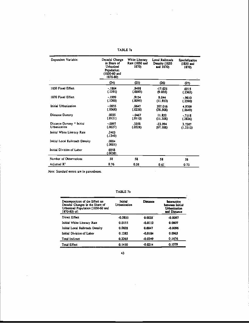
TABLE 7a

Dependent Variable: Decadal Changein Share ofUrbanizedPopulation:

(1850-60 and1870-80)

White LiteracyRate (1850 and

1870)

Local RailroadsDensity (1850

and 1870)

Specialization(1850 and

1870)

.

(24) (25) (26) (27)1850 Fixed Effect -.1864

(.1291).9498

(.0089)-17.025(9.035)

.0215(.2365)

1870 Fixed Effect -.1999(.1260)

.9154(.0099)

9.044(11.923)

-.9610(.2390)

Initial Urbanization -.0855(.0368)

.0641(.0238)

207.016(28.508)

4.9709(.5649)

Distance Dummy .0035(.0121)

-.0467(.0110)

I 1.852(11.30$)

-.7118(.2826)

Distance Dummy • InitialUrbanization

-.0097(.0627)

3358(.0528)

-23.994(67.188)

3.7387(1.2313)

Initial White Literacy Raze .2403(.1349)

Initial Local Railroads Density .0004(.0001)

Initial Division of Labor .0258(.0050)

Number of Observations 58 53 58 58

Adjusted R 0.76 0.58 0.61 0.73

Note: Standard errors are in parentheses,

TABLE lb

Decomposition of the Effect onDecadal Chacs in the Share of

InitialUrbanization

Distance Iratetactionbetween Initial

Urbanized Population (1850-60 and1670-80) of: •

Urbanizationand Distance

Direct Effect -0.0855 0.0035 40097Initial White Literacy Raze 0.0155 -0.0212 0.0*07

Initial Local Railroads Density 0.0828 0.0047 -0.0096

Initial Division of Labor 0.1282 -0.0184 0.0965

Total Indirect 0.2265 -0.0249 0.1676

Total Effect 0.1410 4.0214 0.1579

43

TABLE 8a

Depeadeac Variable: Log of PerCapita GD? in1960 and 1985

.

Change In Iog ofPeneaiage

PopulatIon withComplete Secondary

Sefloollag(I%0-

Change In Logof CapitalStock perCapita

(1960-85)

Ozange inresidual

from regressio(28)

(28) (29) (30) (31)

Intercept 2.6945(.3000)

-.0693(.2154)

-1.2990(.1715)

1960 Fixed Effect -4.01 16(.3061)

1985 Fixed Effect 4.0206(.2990)

Log of 1960 Complete SecondarySchooling

.0540(.0304)

Log of 1960 Capital Stock perCapita

.5662(.0322)

1960 Extent of the Market -54.7697(11.416)

32.052(8.1966)

56.271(6.5291)

Number of Observations lOS 54 54 54

Adjusted R' 0.81 0.29 0.21 0.58

Note: Standard errors are in parentheses.

TABLE Sb

Decomposition of the Effect onLog of Per Capita GD? Changes(1960-85) of:

Extent of the Market

Growth of Human Capital Channel -2.96

Growth of Physical InfrastructureChannel

18.15

Unexplained Increase inProductivity

56.27

Total Effect 71.46

44

TABLE 9a

Dependent Variable: Urbanizationin 1850, 1860,1870 and 1880

DecadalChan;e in

WhiteLiteracy Rate(1850-60 and

1870-80)

DecatlalChange in

LocalRailroadsDensity

(1850-60 and1870-80)

DecadalChange InResidual

fromregression

(32)

(32) (33) (34) (35)

ISSOFixedEffect -1.1584(.3357)

.0090(.0018)

21.764(3.364)

-.0026(.0098)

1860 Fixed Effect -1.1880(.3352)

1870 Fixed Effect -1.1568(.3260)

.0127(.0018)

16.049(3.723)

-.0068(.0088)

1880 Fixed Effect -1.2118(.3255)

ContemporaneousWbite Literacy Rate

1.3288(.3565)

ContemporaneousLocal Railroads Density

.0026(.00026)

ContemporaneousExtent of the Market

-.1279(.0425)

431.80(86.3 13)

.2025(.2082)

Number of Observations 116 58 58 58

Adjusted R' 0.64 0.08 0.25 -0.02

Note: Standard errors are in parentheses.

TABLE 9b

Decomposition of the Effect onDecadal Changes in the Share ofUrbanized Population (1850-60 and1870-80)01:

Extent of the Market

Growth ofHuman Capital Channel

-0.1699

Growth ofPhysical Infrastructure Channel

1.1221.

I

UnexplainedIncrease in Productivity

0.2025

Total Effect 1.1553

45

Appendix 1: 65 country sample

Country CountryCode Name

Algeria3 Benin4 Botswana5 Burundi6 Cameroon7 Central African Republic9 Congo10 Egyptii Ethiopia12 Gabon13 Gambia16 Ivory Coast17 KenyaIS Lesotho19 Liberia20 Madagascar21 Malawi22 Mali23 Mauritania24 Mauritius25 Morocco27 Niger28 Nigeria29 Rwanda30 Senegal31 Sierra Leone32 Somalia34 Sudan36 Tanzania37 Togo38 Tunisia39 Uganda40 Zaire41 Zambia42 Zimbabwe43 Bangladesh46 India51 Jordan52 Korea54 Malaysia55 Nepal56 Pakistan57 Philippines60 Sri Lanka61 Syria63 Thailand71 Greece76 Malta'79 Portugal83 Turkey88 Dominican Republic

46

89 El Salvador90 Guatemalaci Haiti92 Honduras93 Jamaica96 Panama100 Bolivia101 Braid103 Colombia104 Ecuadorlos Guyana306 Paraguay314 Papua New Guinea118 Indonesia

47

Appendix 2: Open and Closed States in the 29 State Sample(using distance from major regional port).

Open Stases

AiabamaConnecticutDelawareLouisianaMarylandMassachusettsMississippiNew JerseyNew YorkPennsylvaniaRhode Island

Cased Siases

ArkansasFloridaGeorgiaIllinoisIndianaIowaKentuckyMaineMichiganMissouriNew HampshireNorth CarolinaOhioSouth CarolinaTennesseeVermontVirginiaWisconsin

48

References

Ades, Alberto, and Edward L. Glaeser (l993) 'Trades and Circuses: Explaining Urban Giants,'mimeographed.

Barro; It. (1991) 'Economic Growth in a Cross-Section of Countries," Quarterly Journal of Economics106: 407444.

Barro, It. and X. Sala i Martin (1992) "Convergence," Jounwi of Politicci Economy 100.

Barn, It. and H. Wolf (1989) tata Appendix for Economic Growth In a Cross-Section of countrIes,"NEER working paper.

Becker, G.S. and K.M. Murphy, (1992) "Human Capital and Speciaiization," Quarterly Journal ofEconomics.

Boldrin, Michele, and José A. Scheinkman (1988). 'Learning-by-doing, International Trade and Growth:A Note, - in Philip W. Anderson, Kenneth Arrow, and David Pines eds., The Economy as anElving Complex System. Reading, MA: Addison-Wesley Publishing Company.

Braun, Juan (1993) 'Essays on Economic Growth and Migration,' Ph.D. Dissertation, HarvardUniversity

Canning, David and Marianne Fay (1993) 'The Effect of Transportation Netwoth on EconomicGrowth,' Discussion Paper, Columbia University, May.

Crowley, Joseph 0. (1992) 'Does Diversity of Production Affect Growth?," Ph.D. Dissertation, HarvardUniversity.

DeLong, B. (1988) 'Productivity Growth, Convergence and Welfare: Comment,' American EconomicReview LXXVIII, 1138-1154.

Easterlin, Richard A. (1960) 'Interregional Differences in Per Capita Income, Population, and TotalIncome, 1840-1950.' In Trends in the American Economy In the Mne:eersth Cetuwy. Princeton,N.J.: Princeton Univ. Press (for NOER).

Glaeser, E., H. KaIlal, J. Scheinkinan and A. Shleifer (1992). "Growth in Cities,' JournoiofrolfticaiEconomy 100.

Glaeser, E., J. Scheinkman and A. Shleifer (1993). "Economic Growth in a Cross-section of Cities,'mimeographed.

Glaeser, Edward L. (1993). 'Why Does Schooling Generate Economic Growth?', Economics Letters,forthcoming.

Grossman, Gene, and E. Helpman (1991). Innovation and Groi&i in the Global Economy. Cambridge,MIT Press.

Historical Statistics of the United States, Colonial Times to 1970 (1976). Wash'mgton: U.S. Dept. ofCommerce, Bureau of the Census.

Keynes, M. (1936). The General Theory of Employment, Inurest, and Money. New York: Harbour

49

Brace Jovanovitch.

lCrugman, P. (1991) 'Increasing Returns and Economic Geography,' Journal of PolLtlcoJ Economy 99:483-499.

Kiugman, p. (1991) Geography and Trade. Cambridge: MIT Press.

KrugTnan P. and R. Livas (1992) 'Trade Policy and the Third World Metropolis', NBER workingpaper #4238.

List, Friedrich (1856) National System of PolitiCal Economy. Philadelphia: Lippincott.

Lucas, R.E. (1988) 'On the Mechanics of Economic Development,' Journal of Monetary Economics 22:3-42.

Mankiw. N. Gregory, David Romer, and David N. WeU (1992). A Contribution to the Empirics ofEconomic Growth,' Quarterly Journal of Economics 107, 401437.

Marshall, A. (1890) Principles of Economics. London: Macmillan.

Murphy. K., A. Shleifer and It. Vishny (1989). industrialization and the Big Push,' Journal of PoliticalEconomy 97: 1003-1026.

Pred, Allan R. (1980). Urban Growth and Cay Systems in the United States, 1840-1880. Cambridge:Harvard University Press.

Pred, Allan It. (1973). Urban Growth arid the Circulation of Information: she United States System ofCities. I7)-l 840. Cambridge. Harvard University Press.

Rae, John (1834) Statement on Some New Principles on the Subject of Political Economy. Boston:Hillard, Gray.

Rebelo, Sergio (1991). 'Long-Run Policy Analysis and Long-Run Growth,' Journal of Pot UIcalEconomy99. 500-521.

Romer, Paul M. (1983). 'Dynamic Competitive Equilibria with ExternaJities, Increasing Returns andUnbounded Growth,' Ph.D. Dissertation, University of Chicago.

Romer, Paul M. (1986). 'Increasing Returns and Long-Run Growth.' Journal of Political Economy 94,1002-37.

Rosenstein-Rodan, Paul N. (1943). 'Problems of Industrialization of Eastern and South-eastern Europe.'EconomicJournal 53, June-September.

Simon, Curtis and P. Nardinelli (1993). 'Information and the Rise of Cities,' unpublished manuscript.

Smith, Adam (1976). An Inquiry into the Nature and Causes of the Wealth of Nations. The Universityof Chicago Press.

Sokoloff, K. (1988). 'industrial Activity in Early America: Evidence from Patent Records.' Journal ofEconomic History. Vol. 98, 8 13-842.

Solow, Robert M. (1956). 'A Contribution to the Theory of Economic Growth,' Quarterly Journal of

50

Economics, LXX, 65-94.

StazisticaJ Abstract of the United States, various issues.

Stokey, Nancy L. (1991). 'Human Capital, Product Quality, and Growth,' Quanerlyiossrnal ofEconomIcs 106, 587-616.

Summers, R. and A. Heston (1991) 'The Penn World Table (Mark 5): An Expanded Set of InternationalComparisons, 1950-1988,' Quarterly Journal of EconomIcs 106: 327-368.

United Nations Handbook of International Thde and Development Statistics, various Issues.

Williamson, J. G. (1985) 'Migration and Urbanization,' 'an the Handbook of Dewlopmens Economics,Amsterdam: North-Holland.

Young, Allyn. (1928), 'Increasing Returns and Economic Progress,' Econonalclournoi, XXXVIII,527-42.

Young, Alwin (1991). 'Learning by doing and the Dynamic Effects of International Trade,' QuarterlyJournal of Economics 106, 369-406.

51