NBER WORKING PAPER SERIES

ENDOGENOUS GROWTH, PUBLICCAPITAL, AND THE CONVERGENCE OF

REGIONAL MANUFACTURING INDUSTRIES

Charles R. HultenRobert M. Schwab

Working Paper No. 4538

NATIONAL BUREAU OF ECONOMIC RESEARCH1050 Massachusetts Avenue

Cambridge, MA 02138November, 1993

We thank the National Science Foundation for its support of this research, and Michael Svilarand Andrew Kochera for their excellent work as our research assistants. We also thank AliciaMunndll for providing us with her data on public capital, and Douglas Holtz-Eakin and DaleW. Jorgenson for their valuable comments. This paper is part of NBER's research programin Productivity. Any opinions expressed are those of the authors and not those of theNational Bureau of Economic Research.

NBER Working Paper #4538November 1993

ENDOGENOUS GROWn-I, PUBLICCAPITAL, AND THE CONVERGENCE OF

REGIONAL MANUFACTURING INDUSTRIES

ABSTRACT

Several explanations can be offered for the unbalanced growth of U.S. regional

manufacturing industries in the decades after World War II. The convergence hypothesis

suggests that the success of the South in catching up to the Northeast and Midwest should be

understood by analogy with the economic success of Japan and the rest of the 0-7 in closing

the gap relative to the U.S. as a whole. Endogenous growth theory, on the other hand,

assigns a central role to capital formation, broadly defined. A variant of endogenous growth

theory focuses on investments in public infrastructure as a key determinant of regional

growth. Finally, traditional location theory stresses the evolution of regional supply and

demand and the role of economies of scale and agglomeration.

This paper compares these alternative explanations of U.S. regional growth by testing

their predictions about the productive efficiency of regional manufacturing industries. We

find little evidence that technological convergence explains the regional evolution of U.S.

manufacturing industry, or that endogenous growth was an important factor. We also find

little evidence that public capital externalities played a significant role in explaining the

relative success of industries in the South and West. The main engine of differential regional

manufacturing growth over the period 1970-86 seems to be inter-regional flows of capital and

labor. The growth of multifactor productivity is essentially uniform across regions, although

there is some variation in the initial levels of efficiency.

Charles R. Hulten Robert M. SchwabDepartment of Economics Department of EconomicsUniversity of Maryland University of MarylandTydings Hall Tydings HallCollege Park, MD 20742 College Park, MD 20742and NBER

I. Introduction

The American South started the post World War II era as the poorest

region of the country. Per capita disposable income was less than 70 percent

of the national level and the South produced less.than 13 percent of national

manufacturing output at that time. However, during the ensuing 40 years, the

South grew much faster than the most of the rest of the nation. As a result,

incomes in the South are now 90 percent of the national average and the South

now produces 22 percent of all manufacturing output.

Several explanations have been offered for this pattern of unbalanced

regional growth. The convergence hypothesis postulates an inverse

relationship between the rate of economic growth and the initial level of

economic activity (Barro and Sala—1—Martln 1991, Holtz—Eakin 1991).1 In this

view of growth, backwardness pj se implies a potential advantage that can

allow lagging regions to catch up to the leaders. Applied to the U.S. , the

convergence hypothesis suggests that the success of the U.S. South in catching

up to the Northeast and Midwest should be understood by analogy with the

economic success of Japan and the rest of the G-7 in closing the gap relative

to the U.S. as a whole.

Endogenous growth theory, on the other hand, assigns a central role to

capital formation, which Is broadly defined to include physical, human.

infrastructure, and knowledge capital.2 The rate of growth of any region

depends on the rate of time preference relative to the marginal productivity

of capital, which is assumed to exhibit constant returns to scale Instead of

diminishing returns as in previous neoclassical models. The larger the wedge

between the time rate of discount and the return to Investment, the more rapid

the rate of growth. When applied to U.S. regional growth, this framework

suggests that the lagging economic performance of the South was due to

inadequate capital formation, and the subsequent boom to an increase In the

rate of investment. The work of Garcia—Mila and McGulre (1987), Aschauer

(1989), Munnell (1990), and Morrison and Schwartz (1992) focuses particular

attention on the role of public investment as a determinant of U.S. regional

growth performance.

In contrast to these two explanations, traditional location theory

stresses the evolution of regional Supply and demand and the role of economies

of scale and agglomeration, combined with nation—wide factors like

technological change, aggregate savings, and population growth, as the

determinant of regional location and growth. The recent paper by Krugman

(1991) shows that the location of manufacturing activity can be concentrated

or dispersed among regions depending on the relative strengths of scale

economies, regional demand, and transport costs.

This paper compares these alternative explanations of U.S. regional

growth by testing their predictions about the productive efficiency of

regional manufacturing industries.3 Using 1970—i986 data from the Census and

Annual Survey of Manufactures for the nine Census divisions of the U.S. and

national data from the Bureau of Labor Statistics and Bureau of Economic

Analysis, we estimate the level of multifactor productivity (MFP) in each

region. We then test for technological convergence and endogenous growth

effects associated with infrastructure externalities and increasing returns to

reproducible inputs, against the prediction of conventional regional theory

that the growth rates of technical efficiency are the same across regions

2

(i.e., that any differences in efficiency levels are region—specific and

constant over time). This test has the collateral effect of addressing the

actively debated question of whether or not public capital has a strong impact

on manufacturing productivity.

II. Test1n the Alternative Models

Our tests of the competing theories are derived from the assumption that

there is a Hicks—neutral production function for manufacturing industry within

each region. We assume that manufactured goods in region I in year t,

are produced using privately owned capital Kit. labor Lit. intermediate

inputs M.t. and public Capital

i A1t(1) = A10 Bj.t e 'F [Kit. L.t, Bit].

Our specification of the public capital variable follows Meade (1952) and

Berndt and Hansson (1991) in identifying two ways that public capital

Influences output. First, it yields direct productive services and thus

appears as an argument of F1[] (as, for example, when trucks and drivers are

combined with public highways to produce transportation services). Second,

public capital acts as an "environmental factor or 'systems spillover which

erthances the productivity of some or all of the private inputs. Thus

appears as an argument of the technical efficiency term in constant elasticity

3

form, where the parameter measures the strength of the within region

spillover effect. This formulation of (I) also assumes that the spillover

effect is separable from the pure technical effect, as represented by the

parameter A1. A10 Is the index of the level of regional productive efficiency

in the base year

A. Technological Convergence

One variant of the convergence model stresses the importance of

technological diffusion. The model of Dowrick and Nguyen (1989) assumes that

nations with low levels of technical efficiency can, at some point In their

history, become open to outside technological possibilities and can thus

appropriate the existing technologies of advanced countries at a faster rate

than the advanced nations can develop new technology. This mechanism is found

by Dowrick and Nguyen to be an important source of cross-national growth

differentials. Applied to regional growth within the U.S. , this variant of

the convergence model assumes that technological backwardness is an important

source of lagging economic performance, and focuses on diffusion of technology

as a process through which regional disparities are reduced or eliminated.

The technological convergence formulation assumes that regional

technologies exhibit initial differences in the level of technical efficiency

in some base year, A10, and that the gap between the level of efficiency In

any region i and the level of technical efficiency in the most advanced

region, Aot closes with a speed of convergence 0:

4

(2) in Ait - in A10 = (1(10)t)(1Aot_ in Arn).

In (2), the growth rate of Ait exceeds that of the leader, but the two

converge over time. This provides the lagging region with an extra Impetus to

output growth.

If the pattern of regional growth is influenced by (2), we should observe

that regional rates of technical change. Xi, estimated from (1) should vary

inversely across regions according to the initial level of efficiency, A10.

On the other hand, if the A1 do not vary across regions there is no

possibility of convergence and either the fl. must be zero or the initial

levels A10 must be equal. In either case, technological convergence cannot be

adduced as an explanation of regional growth differentials In U.S.

manufacturing Industry.

B. Endogenous Growth Models

The endogenous growth literature has two principal branches: the "AK'

model developed by Rebelo (1991) and the externality-increasing returns model

of Romer (1986) and Lucas (1988). Both emphasize the importance of increasing

returns to scale generated by reproducible capital inputs and both predict

noriconvergent rates of growth. In the 'AK model, constant returns to capital

input is imposed directly and growth differentials depend on the wedge between

the marginal product of capital A1 and the rate of time discount p1. To

explain regional growth patterns, each region must be treated as a separate

economy with its own Ai and p1. Regional differences in marginal products may

5

occur because of locational advantages, differences In region specific

capital, or region specific externalities generated by capital. Regional

differences In the propensity to invest that are driven by differences in the

propensity to save (p1) are more difficult to rationalize in an economy which

Is open to capital flows, but this is a problem common to many growth models,

Including Solow—type convergence models.

The Rebelo—Romer-Lucas mechanism of endogenous growth theory is based on

constant marginal returns to capital generated by capital related spillovers.

This may occur because of "within—region" externalities or, following Barro

(1990) and Barro and Sala I Martin (1992), because public capital is fixed by

policy at a constant fraction of the private capital stock, I.e., Bit =

Kit. In this last case, the Romer—Lucas production function might be written

as

a1 a1+1 .= AIO[Bit Kit Lit = A10 tiKit L1

If a.+ f3 equals one, private producers perceive that production takes place

under constant returns to scale and a competitive equilibrium may be

established. However, because public capital enhances production and because

it is proportional to private capital, the true elasticity of output with

respect to capital is a1+ s',, and there are increasing returns to scale (the

further restriction a1+ = I yields the "AX" model).

The endogenous growth formulation of technology (3) is clearly a special

case of the production function (1), in which F'1(') has the Cobb-Douglas form,

disembodied technical change A is zero, and the direct and indirect effects

6

of public capital are collapsed Into the parameter i. Public capital enters

the production function of manufacturing Industries mainly as a service

purchased from other sectors (e.g. , transportation services are reflected In

and thus the direct contribution of Bit is of minor importance.6 In

this case, tests of the parameter are equivalent to tests of the endogenous

growth model. In conjunction with tests of Increasing returns to scale.

C. Location Theory

Location theory does not have the kind of analytical unity that

characterizes the two convergence and endogenous growth hypotheses (see, for

example, Krugman 1993). It is hard to formalize a parametric test of the

theory," so we will only observe that location models typically put more

emphasis on regional or spatial factors, increasing returns to scale

(i.e., agglomeration economies), etc. There is no reliance on regional

differences in technology as an explanation of growth differentials except.

perhaps, those introduced by differences in industry mix across regions. This

leads to the expectation that the manufacturing production function for each

region should have the same degree of technical efficiency, or A = Ait = .

= in each year t. We can test this hypothesis using the parameters of

(1), since a common technology implies A00 = A10= .. = A. and the equality

of the technical change parameters. A1. And, as shown below, we can also test

for increasing returns to scale.

7

III. The Sources of Growth Framework

Since our tests of the competing models primarily Involve the efficiency

term in the production function, it is unnecessary to estimate all of the

parameters of the structure of production. Instead, the relevant tests can be

based on a two stage procedure that makes use of nonparametric index number

techniques. The first step involves the computation of the Solow residual

under the assumption that public capital has no effect on private output

growth.7 The continuous time version of the Solow residual has the form:

L(4) = mjtKjt— itL1t — ntMit

where hats over variables denote rates of growth and the are income

shares.

In practice, the rate of productivity growth is estimated by replacing

logarithmic differentials with differences In successive logarithms and using

average shares:

(5) ln At - in Ati = in — in— 1/2 (nK + i) (in Kit — in

Kit_i)

- 1/2 (tL + n- (in Lit - in L.1)— 1/2 (m + 1rt) (in — in Mti).

This approximation places only weak restrictions on the functional form of the

underlying production function (Diewert 1976) and, in particular, is not

8

restricted to the Cobb-Douglas form. However, Hicks—neutral technical change

is assumed (Hulten 1973). Each term in (5), except the growth rate of the

Solow residual, can in principle be measured directly, and the growth rate of

the technology Index can thus be estimated as a residual.

Jorgenson and Nishimizu (1978), Denny, Fuss, and May (1981), and

Christensen, Cummings, and Jorgenson (1981) have shown that this sources of

growth model can be extended to estimate differences in the level of

productivity across regions or countries. In their framework, the difference

between the level of technology in region i at time t and region j at time s

equals the logarithmic differences in output minus the share weighted

logarithmic differences In inputs, where the shares are the simple averages of

the shares in the two regions. Thus the level Index analog to (5) is

S S(6) in Ait — in

A15= ln it — ln

0,Js

K K- 1/2 (it + n ) (ln K — ln Kit .js it jsL L— 1/2 (Ttit + Js (in Lit — in

L1)H M— 1/2

(ira + flj) (ln Hit — inM15).

SThe resulting levels indexes, Ait. are expressed relative to the efficiency of

the "base" region in the base year, A0 = 1. We have used the U.S total and

1970 as the base region and year, and thus all of the productivity index

numbers should be interpreted as a proportion of national productivity in

1970.8

After calculating the regional Solow level index numbers using equation

(6), we then link measured productivity to the technical efficiency terms in

9

the underlying production function (1) in the second stage of the analysis.

The true growth rate of efficiency is derived from (1) and equals

L(7) Ait = liBit +

A1t= — citKit — cit1i —

where is is the elasticity of output with respect to Input X.

A comparison of the Solow residual At with the true efficiency tern

Ait reveals that public capital's contribution to output has been ignored

and that the income shares are assumed equal to the corresponding

Output elasticities c. This second assumption does not pose a problem for

income shares of the variable private factors (labor and Intermediate input)

when the economy is in competitive equilibrium and they are paid the value of

K Ktheir marginal products. However, it Is not true that = it in general

even under competitive assumptions. The problem arises because the price of

Kcapital services, P1k, can rarely be observed directly. Therefore, capital

income is usually imputed from the 'addlng—up' condition that factor payments

exhaust total income, with capital income measured as the residual. The

residual measurement of capital income therefore imposes the condition that

K L Mincome shares sum to one (i.e., = 1 — — na). Thus whenever the

K L Helasticity of scale of private inputs c1 = + is different from

Kone. misstates Capital s true output elasticity.

These various sources of bias can, however, be accounted for explicitly

to yield an exact relation between the growth rate of the Solow residual and

the true efficiency term. With some manipulation, it can be shown that

10

B(8) Ait = Ait + + c11 Bit +

—

where is the scale elasticity. This expression Indicates that the growth

rate of the measured Solow residual Is the sum of three factors: (i) the rate

of growth of public capital weighted by the indirect and direct contributions

of public capital, (ii) the growth rate of private capital weighted by a

correction for any error that is introduced by the assumption of constant

returns to scale in private inputs, and (iii) the true growth rate of

technical progress.

Equation (8) relates the growth of the Solow residual to its component

elements and forms the empirical basis for our test of the various theories of

regional growth (variants of (8) are also the basis for the marginal cost

mark—up model of Hall (1988) and the externality model of Caballero and Lyons

(1990a, 1990b). However, since the convergence hypothesis involves the level

of technical efficiency rather than its growth rate, one final step Is needed

to complete the second stage our analysis. By assuming that , c, c1, and

A. are constant over time, we can integrate (8) over time to obtain9

(9) ln At = in A0 + A1t 'i + c] ln +[c1

— 1] ln Kit.

The various hypotheses discussed above are special cases of this equation, and

we will therefore use the stochastic version of (9) in the empirical work

presented below.10

11

IV. Data

The data needed to estimate the parameters of equation (9) are described

in full in our earlier papers (Hulten and Schwab 1984, 1991). Our analysis is

restricted to manufacturing industries. Most of our regional data were

obtained from the Census of Manufactures and the Annual Survey of Manufactures

and then reconciled to Bureau of Labor Statistics totals. We use gross Output

as our measure of output In this paper, and thus our private inputs include

capital, labor, and intermediate inputs (corrected for the purchased services

problem). Since regional output deflators are not available from any source,

we have used the national deflators from the U.S. Bureau of Labor Statistics.

This introduces a potential bias in our results, since any error in the price

deflator translates directly into an error in measuring real output and thus

into an error in measuring the left hand side of (9)•hl

Our data on public capital are the same as those used in Munnell (1990);

a full description of the data are included in Appendix A of that paper.

Briefly, Munnell used annual data on state capital outlays to allocate BEA

estimates of the national stock of public capital among the states. Her data

set includes estimates of total public capital for each state as well as

separate estimates of state stocks of highways and water and sewer facilities.

Since the Munnell data are available only for the period 1970-1986, our

analysis is limited to those years.

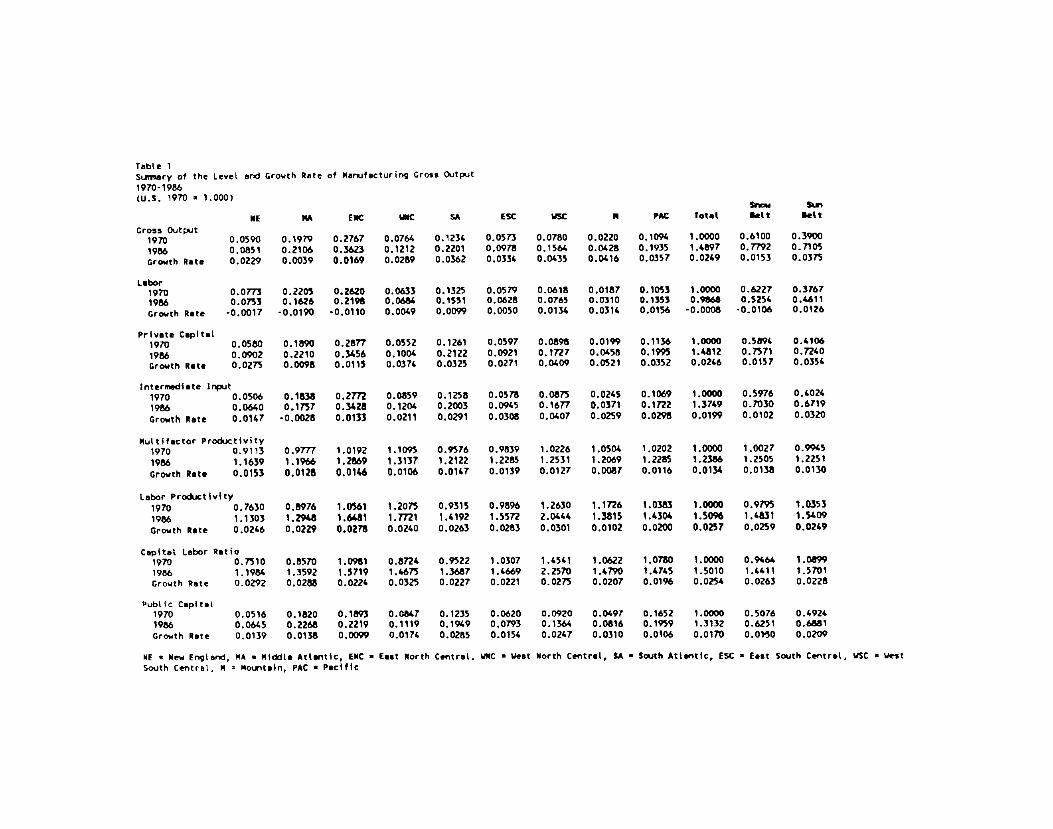
Table 1 presents summary statistics on our measures of manufacturing

input, output, and the Solos., residual. Table I also includes summary

statistics on regional Output per worker, capital per worker, and public

12

capital. It Is clear from this table that the manufacturing sector grew much

faster In the South and West . Gross output rose 3.75 percent per year in the

Sun Belt during the 1970—1986 period as compared to only 1.53 percent per year

in the Snow Belt.12 Labor input grew by more than 1 percent per year in the

Sun Belt but fell in the Snow Belt. Public capital grew more rapidly in the

Sun Belt (2.09 versus 1.30 percent).

It is highly significant for our subsequent analysis that the

differential grow rates of regional output were due almost entirely to the

differential growth in inputs. Regional differences in the growth rates of

the Solow residual (MFP) were relatively small, with the Snow Belt actually

enjoying a slight advantage over the Sun Belt (1.41 percent per year versus

1.23). It was also the case that the level of MFP in the various regions of

the country were very similar at the beginning and end of our sample period.

It is also clear that the growth rates of capital per worker and output per

worker were roughly the same in the Sun Belt and Snow Belt regions over this

period. Our conclusions about MFP convergence during the years 1970—1986 can

thus be extended to the convergence in output per worker due to

capital-deepening. Our data would thus suggest a theory of regional economic

growth that stressed the cross-sectional equality of productivity, prior to

any econometric analysis.

This impression is reinforced by decomposing the total variation of MFP

into variation across time within in regions and variation across regions.

Slightly less than one—half of the the variation in the level of MFP is due to

cross sectional variation, with the balance due to variation over time. For

the growth rates of MFP, however, virtually all of the variation is variation

13

over time, I.e. there is almost no variation in the growth rate of MFP across

regions. Given the substantial differences In the growth rates of public

capital stock in different regions, the lack of variation In the growth rate

of Mfl' suggests that the two variables are essentially uncorrelated.

Table 1 covers a fairly short period 1970—1986, and it is possible that

convergence (in terms of MFP or capital per worker) was essentially complete

by that time. Regional gross output data are not available prior to the

mid-1960s, but regional value added data are available beginning in 1951. In

Table 2. we briefly shift the focus to value added as a measure of output in

order to extend the analysis back in time. That table indicates that there

has been no significant compression (or divergence) in MF'P, in output per

worker, or in capital—deepening since 1951.

V. Econometric Results I: Hypothesis Tests of Competing Models

While the data shown in Tables I and 2 are suggestive, they do not

constitute a formal test of the alternative hypotheses about regional growth.

An econometric test can, however, be obtained by estimating the parameters of

the system of nine linear eqi.ations, each relating the natural logarithms of

the level of regional Mn' to a constant, the natural log of private capital in

the region, the natural log of public capital and time. In other words, we

implement the model (9) without any parameter restrictions across equations

Moreover, since we use index number procedures to account direct inputs of

capital and labor, we impose no restrictions on the form of F'('). Our paper

14

thus differs from much of the other econometric literature on regional growth,

in which parameters are constrained to be equal across regions, except

possibly for regional fixed effects. Indeed, one of our objectives Is

the validity of the cross—regional parameter restrictions which we have

to be tests of the alternative theories of growth discussed above.

The nesting scheme of the various cross—equation restrictions Is shown in

regional technical change exhibits neither convergence nor divergence. R3 and

test whether the MFP elasticity of public capital and the scale elasticity

of private Inputs are zero in all regions, and thus test for endogenous growth

effects associated with public and private capital, respectively (I.e. , test

for the importance of public capital externalities and increasing returns to

scale in private inputs).

The boxes on the third level test whether the restrictions on the second

level can be Imposed jointly, two at a time. There are six possibilities for

these pair wise restrictions: R12, the initial levels of MFP are equal (R1)

and the growth rates of technical change are also equal (R2). letting the

to test

shown

Figure 1. The box at the top level represents

(9) is estimated without any parameter restrict

boxes on the next line represent, respectively,

each of four sets of parameters (designated R1,

equality across regions of the intercept of the

other parameters to vary, and thereby tests for

among the regions. Similarly, the restrictions

the regional growth rates of technical change

this restriction cannot be rejected, we cannot

the case in which the system

ions (designated R0). The four

the equality restrictions on

R2, R3, R4). R1 tests for the

MFP regressions allowing all

equality of initial MFP levels

in R2 test for the equality of

the coefficients on t). If

reject the hypothesis that

15

r.st

rlctlo

ns:

Equ

.Uty

of

th.

$nt.r

cspt

s

16 r.

.t,to

n,:

snd

Iotd

Jol

nt(y

/

flg..r

e I

4 25

R.,N

ho

\d

R

ie r

.,tX

ctio

n.:

1 25

1,, I, l

)wId

Jbt

nfly

L

1,1,

1 L

I

other parameters vary freely across regions; R13. the initial levels of MFP

are equal (R1) and the elasticity of MFP with respect to public capital are

also equal (R3); and so on for R14r R23, R24, and R34. Only the boxes for

R12 and R34 are shown in Figure 1, for ease of exposition, but these are also

the joint hypotheses of particular interest, since the restrictions of R12

imply identical regional paths for technical change and R34 imply that there

are no endogenous growth effects linked to public or private capital.

The four boxes on the fourth line of Figure 1 show the possible

combinations In which three of the four restrictions hold jointly (they are

designated R123, R134, R124, and R234). Finally, R1234 on the bottom level Is

a test of all the restrictions sinultaneously. If all of the restrictions

hold jointly, the regional paths of MFP are identical and are not influenced

by the amount of public capital in each region, nor by increasing returns to

scale effects. This situation Is, of course, very unfavorable to the

convergence and endogenous growth explanations of the evolution of regional

manufacturing industry in the U.S.

Table 3 presents the sum of squared errors and F statistics associated

with the various possible restrictions. It is apparent from this table that

the data do not reject (at the 1 or 5 percent levels of significance) any of

the restrictions imposed by themselves. If, for example, the public capital

parameter, , is constrained to be zero In each region, the resulting model,

(9') in A = In A. + A t + [c. - 1] ln K.it iD 1 i it

cannot be distinguished from the original (9). Similarly, Table 3 indicates

17

that. rnutatis mutandi, a model that makes A10 or A the same across regions,

or makes (c1 — 1) zero, cannot be distinguished from (9). Further, the data

do not reject any of the pairs of restrictions imposed jointly. It Is Only

when the fourth level of three—way restrictions is reached that one set of

restrictions, R134, Is rejected; the data do not accept the simultaneous

equality of the initial levels of HFP, a zero elasticity of MFP with respect

to public capital, and constant returns to the private inputs, implying that

the model ln At = in A0 + At Is not a valid model. However, all of the

other three-way restriction do hold jointly. Finally, the simultaneous

imposition of all restrictions simultaneously, R1234. is also rejected, so

that in At = ln A0 + At is not an appropriate model.13

Table 3 thus provides very little good news for the convergence or

endogenous growth explanations of regional manufacturing growth. The

predictions of these models simply do not dominate other explanations In which

convergence and endogenous growth play no role.

VI. Econometric Results II: Estimation of Restricted Models

The results presented in Table 3 are compared with a base-line assumption

that all parameters, including the elasticities of MFP with respect to public

and private capital, vary across regions. In this section we approach the

problem from a slightly different point of view by restricting the

elasticities of public and private capital to be equal across regions. This

18

is consistent with the recent literature on regional growth (e.g. , Holtz—Eakiri

1992, Garcia-Mila, McGulre, and Porter 1993, Munnell 1990, and Aschauer 1990)

This shift in perspective make it easier to compare our results to other

recent research. Moreover, because there are so many parameters in the

unrestricted version of the models in the previous section, it is hard to

estimate any particular parameter precisely and to interpret the resulting

coefficients. Finally, restricting the elasticities to be eq.1al across

regions is consistent with the data. As shown in Table 3, we cannot reject

the hypothesis that all of the elasticities with respect to public and private

capital are equal to zero, and thus we certainly cannot reject the hypothesis

that they are all equal to one another.

The results of this alternative approach are shown in Table 4. The first

column of Table 4 reports the results obtained from the estimation of the most

constrained version of these models where the initial level of MFP and the

growth rate of MFP are all assuined to be eqiial across regions. Interestingly,

the results are similar to those found in the earlier literature on public

capital: the coefficient on public capital Is statistically significant and

reasonably large given that the direct effect of public capital is already

accounted for in the purchased service component of F1('). The private

capital coefficient suggests that there are mildly decreasing returns to scale

and the point estimate of the time parameter implies a rate of MFP growth of

0.8 percent per year.

It is common in this literature to include a measure of capacity

utilization in order to control for the cyclical effect of demand fluctuations

on the Solow residual. Many, however, view this practice with some

19

skepticism, As Berndt and Fuss (1986) and Hulten (1986) show, there Is rio

theoretical Justification for Including capacity utilization in a productivity

model since the effects of the business cycle should be reflected in the

output elasticity of private capital. Capacity utilization is particularly

problematical in regional studies since regional capacity utilization measures

are not available.

Setting these concerns aside for the moment, column (5) in Table 4 adds

the Federal Reserve Board's national capacity utilization data for

manufacturin.g to the model in column (1). As shown In column (5), when we add

capacity utilization the picture does not change very much, though the error

sum of squares does fall significantly.

Regional fixed effects are introduced In column (2) by allowing for

separate regional intercepts (New England is taken as the base region). As in

previous studies, the addition of these regional fixed effects causes the

public capital variable to become statistically insignificant (and negative as

well). The same is true for private capital, implying constant returns to

scale. Five of the regional intercepts are significant at conventional

levels, and the rest are marginally significant at low levels. Adding

capacity utilization does not change this picture, except to reduce the sum of

squared errors and Improve the significance of the regional intercepts.

Column (3) allows for regional time effects while holding the intercepts

the same for all regions (I.e., we impose a common level of MFP at the outset

to see if the times paths of HFP diverge). We find that this yields a larger

estimate of the public capital coefficient than the base case of column (1),

and that it implies strongly decreasing returns to scale. Half of the

20

regional time effects are significant. As before, adding capacity utilization

does not change the results,

The last step taken In Table 4 Is to go beyond the fixed effects model

and allow both the Intercepts and time coefficients to vary across regions.

The results, shown in column (4), are consistent with the fixed effects model

of column (2): the public and private capital variables are insignificant,

half of the intercept dummy variables are significant, and none of the

regional time dummies are significant. However, the addition of the capacity

utilization variable does make a difference. When It is included, the public

capital coefficient is significantly negative, Implying that public capital

externalities reduce KFP with an elasticity of —.24. This is a highly

implausible result, and it casts doubt on the usefulness of using an aggregate

capacity utilization adjustment.

How do the results of Table 4 accord with the hypothesis tests of the

preceding table? The constraints imposed in Table 4 on the public and private

capital parameters only restrict them to be equal, and not to be equal to zero

as in Table 3. Moreover, Table 3 considers a wider range of parameter

restrictions (i.e.. on the time variable). However, with these differences in

mind, it is clear that the proceeding up the hypothesis tree In Figure 1 using

Table 4 F—statistics produces similar conclusions about the models that the

data wants to reject (i.e., some difference in initial levels, no difference

in the growth rates of MFP, and no effect of public capital).

We note, finally, that we tested several variants of the our models.

Following Fernald (1992), we carried out an analysis of (9) using deviations

from time trend rather than the log—level of variables in order to control for

21

demand fluctuations and to reduce any simultaneous equation bias resulting

from the endogenelty of K and B. The results of this exercise were similar to

the results obtained using the capacity utilization variable.

We also tested the assumption of perfect Competition using a Hall (1988)

marginal cost mark—up model. In an imperfectly competitive market where the

ratio of price to marginal cost is a constant . the income shares of labor

and intermediate input are equal to the true output elasticities divided by i

L L M H(i.e., / i and = / ii). If capital s share is calculated as

a residual so the shares sum to 1, then it is not difficult to show that

Hall's model implies that (9) ecomes

(9") lri At in A.0 + )t + + c] ln B.t + [ci — 11 in K.t

+ (i — 1) [1t1n (M.t / K.) + (Lit /

We estimate this model by including the share weighted log of the intermediate

Input—capital and the labor—capital ratios to the models shown in Table 4. As

shown in equation (9"), the coefficient on this variable represents an

estimate of (.t — 1). Under perfect competition price equals marginal cost, p

eqials 1, and the coefficient on 1Tln (Hit / Kit) I (Lit / Kit) will

equal zero; if firas have market power then price will exceed marginal cost

and this coefficient will be positive.

Estimates of different versions of this Hall model are shown in Table 5.

In those specifications where we include capacity utilization variable, our

estimate of (i — 1) is always positive and significant; in those

specifications where we exclude capacity utilization variable, our estimate of

22

(.z — 1) Is always Insignificant. Estimates of all of the other parameters In

Table S are quite similar to the corresponding estimates in Table 4.

VII. Conclusions

This paper has proposed a framework for testing three of the leading

explanations of comparative regional growth based on different predictions

about the times paths of technical efficiency. While the tests are limited

to the manufacturing industry and not all of the variants of the competing

theories are tested, the tests do provide evidence against two of the major

competitors. Specifically, the absence of MFP convergence or divergence is

not compatible with the predictions of the technological convergence or

endogenous growth models. Moreover, an inspection of the trends in Output per

worker and capital per worker for the 1970-86 and the 1951-86 periods using

different output concepts does not offer any encouragement for the

capital—deepening variant of the convergence hypothesis.

We have also found that the externalities associated with public capital

are, for the most part, not statistically significant and the point estimates

of the elasticity of KFP with respect to public capital in some versions of

the model are negative. Of course, this applies only to manufacturing, but it

lends little support to the argument that public capital externalities are an

important engine of growth. If externalities are not significant in this

important sector, where do they play an important role in regional economic

development?

23

We also find that manufacturing is subject to constant returns to scale

at the regional level. This result suggests that agglomeration economies may

play only a limited role in regional economic growth.

Our findings suggest that manufacturing industry was open to flows of

capital, labor, and technology, and this is more congenial to the traditional

equilibrium approach to location theory than to the other two models which are

imported from international growth analysis. The main engine of differential

regional manufacturing growth over the period 1970-86 seems to be

inter—regional flows of capital and labor, while the growth of multifactor

productivity Is essentially uniform across regions (although there appears to

be some variation In the initial levels of efficiency).

Several aspects of our results deserve emphasis in this summing up.

First, the statistical results reported above refer to a relatively short, and

recent, time period: 1970—86. It may well be the case that technological

convergence and public capital externalities were important in an earlier

stage of U.S. regional development. However, our estimates of a limited

version of our model for the period 1951—86 (which by necessity could not

consider public capital and relied on value added rather than gross output)

yielded virtually the same results. Second. it cannot be emphasized too

strongly that we have assumed that the Law of One Price holds. If there is

significant regional variation in the deflators used to estimate real output,

our results could be dramatically altered.

Third, our finding that public capital externalities were not an

important source of regional manufacturing growth does not mean that public

capital formation is irrelevant. It may well have played an essential role In

24

facilitating the movement of capital, labor, and intermediate inputs which we

find are the main sources of differential regional growth. Furthermore,

because the impact of lumpy infrastructure projects like the Interstate

Highway System may be highly non-linear, there may be extended periods during

which the average product of public capital Is high but Its marginal product

Is almost zero. But, even with these caveats, our results are relevant for

the question of whether undetected externalities might thus have led

governments to supply too little public capital In recent years. We find no

evidence of under-supply in the regional manufacturing data.

25

Notes

1

As noted by Baumol (1986), the convergence hypothesis has a long traditionand an extensive literature. Recent contributions include Dollar and Wolff(1988), De Long (1988), Bauinol et. al. (1989), Barro (1991), and ?lankiw, Romerand Well (1990).

2The endogenous growth model was developed by Romer (1986), Lucas (1988),

and Rebelo (1991). The survey by Sala-i—Martin (1990a, 1990b) provides anextensive description of the main variants of the endogenous growth model andtheir relation to optimal growth theory.

Our focus on regional manufactur1n industry Is motivated in part by theimportance on manufacturing in the regional model developed by Krugman (1991).and also by the fact that data on inputs and output are better for this sectorof the economy. However, the narrower industrial focus of this paper meansthat our results are not strictly comparable to those based on broadermeasures of regional output such as total private gross state product.

This specification of the public capital externality assumes that the onlysource of spillovers in each region is the quantity of public capital withinthat region. This reflects the assumption that the highway system of oneregion gives rise to positive spillovers, but the highways of an adjacentregion have no effect at all. This is consistent with our interpretation ofthe region specific externalities as an engine of regionally endogenousgrowth. However, It is also possible that public capital externalitiesaffect all regions, in which case the relevant argument of A[1 would be

total public capital, Bt = or a vector of the public capital in all

regions.

26

It should be noted that the literature on convergence theory has twodistinct branches: the one described above and another in which convergencetakes place as a country or region moves to Its steady—state rate of growth bycapital deepening. When the production function has the form = kt. the

convergence equation is given by an equation similar to (2):

(2') in - in q = (1(1)t)(1 - inq0),

where ' = (1-a)i is the speed of convergence parameter (Holtz-Eakln (1991),following Mankiw, Romer, and Well (1990)). With labor— augmenting technicalprogress at a rate A, the steady state values of output and capital per "raw"worker will grow at the rate of technical change, and the speed of convergenceparameter becomes i (1—a)(T1+A). This is the approach taken by Barro andSala—l-Martin (1991) and Holtz—Eakin (1991), and both studies find aconvergence effect within the regions of the U.S. In this Interpretation, theolder industrial regions of the U.S. experienced slower growth than the Southand West because the older regions were further along in the convergenceprocess and closer to their balanced growth paths. This interpretation hasbeen challenged by Blanchard (1991), who demonstrates that the convergenceequation (2' ) can be derived from the spatial equilibrium model and shows thatthe convergence parameter of their estimating equation can equally beInterpreted as a demand elasticity. We will not attempt an econometric testof (2' ) in this paper, but will comment on Its applicability In our section onregional data.

6According to BLS data, trucks and autos accounted for approximately 8

percent of the income accruing to equipment in manufacturing, and thus aboutone percent of the total income, over the period 1949—83, and thatcommunications and electricity generation equipment, which account for about 9percent of income accruing to equipment, and, again, about one percent oftotal income. This low share reflects the fact that public capital Is mainlyan input to the transportation and communication sectors, to public utilities,and to some service industries, and these sectors pass along their services(and thus the services of public capital) by selling their output tomanufacturing industries. Thus, public capital is at best a marginalcontributor to the gross Output of many industries.

27

This mode of analysis, also termed sources of growth analysis." wasdeveloped by Solow (1957), Kendrick (1961), Denlson (1962). and Jorgenson andGrlliches (1967). It is the conceptual basis of the recent studies by theU.S. Bureau of Labor Statistics (1983) and Jorgenson, Gollop, and Frauineril

(1987), and is the framework used in our 1984 and 1991 studies of regionaleconomic growth, The sources of growth analysis has, for the most part.Ignored the role of public capital as a source of output growth.

8 All growth rates are the continuous growth rates of the level Solow indexnumbers.

The constancy of these parameters imposes restrictions on the underlyingtechnical efficiency function in (1): if, for example, the elasticity ofscale is constant at c, the production function is homogeneous of degree c.Note, however, that the multiplicative restrictions on the form of theefficiency function does not Impose restrictions on the rest of the

technology, F('). In particular, they do not imply that the productionfunction has the Cobb—Douglas form.

10An econometric problem that arises when estimating (9) using ordinary least

squares should be noted. Private capital (and possibly public capital aswell), are endogenously determined and thus may be correlated with the errorterm in the regression. Instrumental variables might be used to avoidsimultaneous equations bias, but a set of valid regional instruments is hard

to find.

If the Law of One Price does not hold for manufactured goods within theU.S. market and there is in fact regional variation in output prices, ourassumption of one price will overstate real output in those regions whereprices are higher than average. This, in turn, overstates the level index ofthe Solow residual. If, in addition, the regional output prices are changingrelative to the average, a bias is introduced into the growth rate of theSolow residual as well.

12 Throughout the paper, we define the Snow Belt as the New England, MiddleAtlantic, East North Central, and West North Central Census divisions. TheSun Belt includes the South Atlantic, East South Central, West South Central,Mountain, and Pacific divisions.

28

13i a 5 percent level of significance is used In the tests of first level of

hypotheses (R1, R2, etc.) then a different level of significance should be

used in tests of the Joint hypotheses. An approximate significance on 20

percent would, for example, be assigned to R1234, by the Bonferroni

inequality (See Savln 1984).

29

Bibliography

Aschauer, David A. (1989). "Is Public Expenditure Productive?,' Journal ofMonetary Economics, 23, 177-200.

Aschauer, David A. (1990). "Why Is Infrastructure Important?," in Alicia H.Munnell (ed.), j There a Shortfall in Public Capital Investment?,Federal Reserve Bank of Boston, Boston, 21—50.

Barro, Robert J. (1990). "Government Spending in a Simple Model of EndogenousGrowth," Journal of Political Economy, 98, Pt. 2, S103-Si25.

Barro, Robert J. (1991). "Economic Growth in a Cross Section of Countries,The Quarterly Journal of Economics, 106, 407—443.

Barro, Robert J. and Xavier Sala—1-Martin (1991). "Convergence Across Statesand Regions", Brookings Papers on Economic Activity, No. 1, 107—158.

Baumol, William J. (1986). "Productivity Growth, Convergence, and Welfare:What the Long Data Show," American Economic Review, 76, 1072—1085.

Baumol, William i., Sue A.B. Blackman, and Edward N. Wolff, (1989).Productivity and American Leadership: The View, The MIT Press,

Cambridge Massachusetts.

Berndt, Ernst R. and Bengt Hansson (i99). "Measuring the Contribution ofPublic Infrastructure Capital in Sweden," The Scandinavian Journalof Economics, 94 (supplement), S151—S168.

Blanchard, Olivier J. (1991). "Comments on 'Convergence Across Statesand Regions," Brookings Papers on Economic Activity, No. 1, 159—174.

Caballero, R. and R. Lyons (1990a). "The Role of Externalities in U.S.Manufacturing," National Bureau of Economic Research Working Paper No.3033.

Caballero, R. and R. Lyons (1990b). "Internal and External Economies inEuropean Industries," European Economic Review.

Christensen, Laurits R., Diane Cummings, and Dale W. Jorgenson (1981)."Relative Productivity Levels, 1947—1973: An International Comparison."European Economic Review, 16, 61—94.

De Long, J. Bradford (1988). "Productivity Growth, Convergence, and Welfare:Comment," American Economic Review, 78, 1138—1154.

Denison, Edward F. (1962). The Sources of Economic Growth in the UnitedStates and the Alternatives before Us, New York, Committee for Economic

Development.

30

Denny, Michael, Melvyn Fuss, and J.D. May (1981). "Intertemporal Changes InRegional Productivity in Canadian Manufacturing," Canadian Journal ofEconomics, 14, 390—408.

Diewert, W. Erwin (1976). "Exact and Superlative Index Numbers," Journal ofEconometrics, 4, 115—145.

Dowrick, Steve and Duc—Tho Nguyen (1989). "OECD Comparative Economic Growth1950—85: Catch—up and Convergence," The American Review, 79, 1010—1030.

Garcia—Mila, Teresa arid Therese J. McGulre, "The Contribution of PubliclyProvided Inputs to States' Economies," Journal of Regional Science.

forthcoming.

Hall, Robert E. "The Relation between Price and Marginal Cost in U.S.Industry," Journal of Political Economy, 96, 921—947.

Holtz-Eakin, Douglas (1991). "Solow and the States: Capital Accumulation,Productivity and Economic Growth," Syracuse University working paper.

Holtz—Eakin, Douglas (1992). "Public Sector Capital and the ProductivityPuzzle," National Bureau of Economic Research Working Paper No. 4144.

Hulten, Charles R. (1973). "Divisia Index Numbers," Econometrlca, 41.1017-1025.

Hulten, Charles R. and Robert H. Schwab (1991). "Public Capital Formationand the Growth of Regional Manufacturing Industries," National TaxJournal, December, 121—134.

Hulten, Charles R. and Robert H. Schwab (1984). "Regional Productivity Growthin U.S. Manufacturing: 1951—1978," American Economic Review, 1984, 74,152-162.

Jorgenson, Dale W., Frank Gollop and Barbara Fraumenl (1987). Productivityand U.S. Economic Growth, Harvard University Press, Cambridge.

Jorgenson, Dale W. and ZvI Griliches (1967). "The Explanation of ProductivityChange," Review of Economic Studies, 34, 249—283.

Jorgenson, Dale W. and Mieko Nishimizu (1978). "U.S. and Japanese EconomicGrowth, 1952—1874: An International Comparison," The Economic Journal,

88, 707—726.

Kendrick, John, (1961). ProductivIty Trends In the United States, NationalBureau of Economic Research, New York.

Krugman, Paul (1991). "Increasing Returns and Economic Geography," Journal ofPolitical Economy. 99, 483—499.

Krugman, Paul (1993). "On the Relationship Between Trade Theory and LocationTheory," Review of International Economics, 1, June, 111-122.

31

Lucas, Robert E. Jr. (1988). "On the Mechanics of Economic Development,"Journal of Monetary EconomIcs, 22, 3-42,

Mankiw, N. Gregory, David Romer, and David N. Well (1990). 'A Contributionto the Empirics of Economic Growth," National Bureau of Economic

Research. Cambridge Massachusetts.

Meade, James E. (1952). "External Economies and Diseconomies in a CompetitiveSituation," Economic Journal, 62, 54—67.

Morrison, Catherine J. and Amy Ellen Schwartz, "State Infrastructure andEconomic Performance," National Bureau of Economic Research Working Paper

No. 3981, Cambridge Massachusetts, January 1992.

Munnell, Alicia H. (1990). "How Does Public Infrastructure Affect RegionalEconomic Performance?," in Alicia H. Hunneil (ed.), Is There a ShortfallIn Public Capital Investment?, Federal Reserve Bank of Boston, Boston,69—103.

Rebelo, Sergio T. (1991). "Long—Run Policy Analysis and Long-Run Growth,"Journal of Political Economy. Vol. 99, No. 3, 500—521.

Romer, Paul H. (1986). "Increasing Returns and Long—Run Growth," Journalof Political Economy, 94, 1002—1037.

Romer, Paul H. (1990). "Endogenous Technical Change," Journal of PoliticalEconomy, 98, Pt. 2, S71-S102.

Sala—1—Martin, Xavier (1990a). "Lecture Notes on Economic Growth (I):Introduction to the Literature and Neoclassical Models," National Bureauof Economic Research Working Paper 3563, Cambridge Massachusetts.

Sala—i—Martin, Xavier (1990b). "Lecture Notes on Economic Growth (II): FivePrototype Models of Endogenous Growth," National Bureau of EconomicResearch Working Paper 3564, Cambridge Massachusetts.

Savin, N.E. (1984). "Multiple Hypothesis Testing," in Zvi Griliches andMichael D. Intriligator (eds.), Handbook of Econometrics, North Holland,Amsterdam, 827—880.

Solow, Robert H. (1957). "Technical Change and the Aggregate ProductionFunction," Review of Economics and Statistics, 39, 312—320.

U.S. Bureau of Labor Statistics (1983). Trends in Multifactor Productivity1948-81, Bulletin 2178, United States Government Printing Office,

Washington.

32

</ref_section>

Tsbte 1

Srmsry of the Lewel sr Growth Rste of Mars.ifecturlng Gross 0tpt 1970-1986 (U.S. 1970 1.000)

ME EMC IMC SA ESC USC N PC Total. lelt I,(t

Gross 0tput 1970 0.0590 0.1979 0.2767 0.0764 0.1234 0.0573 0.0780 0.0220 0.1094 1.0000 0.6100 0.3900

1986 0.0851 0.2106 0.3623 0.1212 0.2201 0.0978 0.1564 0.0428 0.1935 1.4697 0.7792 0.7105

Growth RIte 0.0229 0.0039 0.0169 0.0289 0.0362 0.0334 0.0435 0.0416 0.0357 0.0249 0.0153 0.0373

LabOr 1970 0.0773 0.2205 0.2620 0.0633 0.1325 0.0579 0.0618 0.0181 0.1053 1.0000 0.6227 0.3767

1986 0.0733 0.1626 0.2196 0.0684 0.1531 0.0628 0.0765 0.0310 0.1333 0.9668 0.5254 0.4611 Growth Rate -0.0017 -0.0190 -0.0110 0.0049 0.0099 0.0050 0.0134 0.0314 0.0156 0.0008 -0.0106 0.0126

Private CapitaL 1970 0.0580 0.1890 0.2877 0.0552 0.1261 0.0591 0.0896 0.0199 0.1136 1.0000 0.5894 0.4106

1966 0.0902 0.2210 0.3456 0.1004 0.2122 0.0921 0.1727 0.0458 0.1995 1.4812 0.7371 0.7240

Growth Rat. 00273 0.0098 0.0115 0.0374 0.0325 0.0271 00409 0.0521 00352 0.0246 0.0157 0.0354

intermediate Input 1970 0.0506 0.1638 0.2712 0.0859 0.1258 0.0576 0.0873 0.0245 0.1069 1.0000 0.5976 0.4024

1986 0.0640 0.1757 0.3428 0.1204 0.2003 0.0945 0.1677 0.0371 0.1722 1.3749 0.7030 0.6719

Growth Rate 0.0147 -0.0028 0.0133 0.0211 0.0291 0.0308 00407 0.0259 0.0296 0.0199 0.0102 0.0320

Multifactor Productivity 1970 0.9113 0.9771 1.0192 1.1095 0.9576 0.9839 1.0226 1.0504 1.0202 1.0000 1.0027 0.9945

1986 L1639 1.1966 1.2869 1.3137 1.2122 1.2255 1.2531 1.2069 1.2285 1.2386 1.2505 1.2251

Growth Ret. 0.0153 0.0128 0.0146 0.0106 0.0147 0.0139 0.0127 0.0087 0.0116 00134 0.0138 0.0130

Labor Productivity 1970 0.7630 0.8976 1.0561 1.2075 0.9315 0.9896 1.2630 1.1726 1.0383 1.0000 0.9795 1.0353

1986 1.1303 1.2948 1.6481 1.7721 1.4192 I .551? 2.0444 1.3815 1.4304 1.5096 1.4831 1.5.409

Growth Rete 0.0246 0.0229 0.0278 0.0240 0.0263 0.0283 0.0301 0.0102 0.0200 0.0257 0.0259 0.0249

Cepitet labor Ratio 1970 0.7310 0.8570 1.0961 0.8724 0.9522 1.0307 1.4541 1.0622 1.0780 1.0000 0.9464 1.0899 1986 1.1984 1.3592 1.5719 1.4613 1.3687 1.4669 2.2570 1.4790 1.4745 1.5010 1.4411 1.5701

Growth Rate 00292 0.0285 0.0224 0.0325 0.0221 0.0221 0.0273 0.0201 0.0196 0.0254 0.0263 0.0228

Public Capital 1970 0.0516 0.1820 0.1893 0.0847 0.1235 0.0620 0.0920 00497 0.1652 1.0000 05076 0.4924 1966 0.0645 0.2268 0.2219 0.1119 0.1949 0.0793 0.1364 0.0816 01959 1.3132 0.6251 0.6881 Growth Rate 0.0139 00138 0.0099 0.0174 0.0285 0.0154 0.0247 0.0310 0.0106 0.0170 0.0150 0.0209

lit Mew Er,lsrs, MA • MlôL. At(.ntic, EPIC — East North Central. WWC • lest Plorth Centrsl SA • South Atlantic, £SC • East South Central, USC • Uest South Central, H = MotJ-ta$n, PAC Pacific

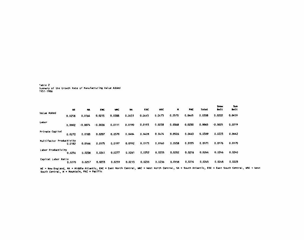
Table 2 Sucriary of the Growth Rate of Manufacturing Value Added

¶ 951 - 1966

NE NA tic i.c SA ESC USC N PAt Total Salt Belt Value Added

0.0258 0.0164 0.0215 0.0338 0.0451 0.0445 0.04Th 0.0570 0.0445 0.0308 0.0222 0.0459

Labor 0.0002 -0.0076 -0.0026 0.0111 0.0190 0.0193 0.0238 0.0368 0.0230 0.0065 -0.0025 0.0219

Private Capital 0.0272 0.0183 0.0207 0.0370 0.0404 0.0428 0.0474 0.0526 0.0443 0.0309 0.0223 0.0442

Multifactor Productivity 0.0182 0.0166 001Th 0.0191 0.0192 0.01fl 0.0160 0.0533 0.0155 0.0111 0.0176 0.0170

Labor Productivity 0.0256 0.0238 0.0261 0.0277 0.0261 0.0252 0.0235 0.0202 0.0216 0.0244 0.0246 0.0240

Capital Labor Ratio

0.0270 0.0257 0.0233 0.0259 0.0213 0.0235 0.0236 0.0158 0.0214 0.0245 0.0248 0.0223

WE a Mew England, MA • Middle Atlantic, (NC a East Worth Central, WNC • Jest Worth Central, SA a South Atlantic, ESC a East South Centrals USC • West

South Central, N a Motmtain, PAC a Pacific

TabLe 3Error Suits of Sqaures and F ft.tist(ca

HYPOtheIIS Error Sue of Squares *estrictL teistiveto

F Stitistic *eItIy.to

PD .14727 .. -•

.15436 8 0.7041

2 .16030 8 1.2940

*3 .16102 9 1.2138

p .16857 9 1.6802

12 .17119 16 1.1877

R. .17977 17 1 .5i

R .17918 17 1.4912

23 .17415 17 1.2562

534 .16093 17 1.5730

534 .16118 18 1.4967

p133 .19732 25 1.5905

24 .19653 25 1.5651.

134 .31317 26 5.0693

*334 .19872 26 1.5721

P334 .58580 34 10.24,59

Tebte 4

Porae,eter Etti,nates of ALternative Restricted ModeLs

(1) (2) (3) (4) (5) (6) (7)

Intercept 0.102214 (3.988)

0.315016 (1.681)

0.126697 (3.533)

-0.660555 (2.037)

-0.378122 (3.880)

-0.910440 (5.912)

-0.351948 (4.979)

•1.42213

-- 0.174645 (2.133)

-- 0.361255 (2.504)

-- 0.223457

(3379) -- 0.476241

(NC - - 0.245769 (3.015)

-• 0.423950 (2.729)

-- 0.283020 (6.558)

-- 0.522270 (4.653)

uwc •- 0.200081 (5.137)

-- 0.278372 (4.846)

-- 0.227019 (7.635)

-- 0.335459 (8.046)

SA -- 0.120506 (1.911)

-- 0215552 (2.253)

-- 0.156855

(3.263)

-- 0.288187 (4.163)

(SC -' 0.087153

(5.088>

-- 0.127440

(4.225)

-- 0.094803 (7.266)

-- 0.140696 (6.466)

usc -- 0195922 (4.797)

-- 0.245046 (4.018)

-- 0.215640 (6.930>

- - 0.288537 (6.542)

MT " 0.060219

(1.591)

-- 0.065613 (0.945)

-- 0.078654 (2.728)

-- 0.081665

PAC -- 0191201 (2.653)

-. 0.338488 (2.787)

-• 0.237179 (6.313)

-- 0.656201 (5.155)

lIme 0.008445 (8.241)

0.010567 (7.225)

0006314 (3.755)

0.015121 (5.448)

0.009906 (9.993)

0.012336

(10.959)

0.007492 (5.225)

0.016974 (8.461)

lIm.MA " " 0002131 (0859)

-0.005766

(1.976)

" -0.001712

(0.814)

-0.005071

TimeENC -- 0007'321 (3.439)

-0.003467

(1.235)

.- 0.007512

(4.163)

(2.412)

-0.003097

lim,WNC •. -- 0.008035 (4.117)

-0.003878

(1.465)

-- -- 0.006342

(5.061)

-0.003497

lIs,5A • -0002247 (1.058)

0.001049 (0.332)

0.001?37

(1.076)

(1.833)

0.003106

TImeFSC -. -- 0.004258 (2.824)

-0.002564 (0.987)

" " 0.004339

(33%)

(1.359)

-0.002015

(1076)

flee*WSC .

" 0.009935 (5.925)

0.002267 (0.746)

-- - 0.010056 (7.073)

0.003223 (1.472)

Te,e*MT -. - -0.000553 (0.393)

-0.002950 (0.867)

-- -- -0.000(68 (0.266)

-0.001322 (0.535)

T%aePAC -- -- 0.001227 (0.520)

-0.004016 (1.515)

-- -- 0.001630 (0.814)

-0.004545 (2.379)

In PthUc Capital

0.0816% (3.526)

-0.036604 (0.472)

0.158439 (4.704)

-0.117309 (1.034)

0.079613 (3.711)

-0.094269 (1.590)

0.150372 (5.263)

-0.244341 (2.961)

In Prvst. C.pIt•

-0.044530

(2.606)

0.046562 (1.029)

-0.105826 (4.556)

-0.076725 (1.094)

0.043099 (2.724)

-0.024187 (0.702)

-0.100636 (5.109)

-0.040135 (0.193)

CapacIty UttUzatlon

-. -- .- — 0.005806 (5.082)

0.005961 (10.191)

0.005731 (7.501)

0.006081 (11.150)

R2 .3661 .7669 .6501 .7906 .4603 .6673 .7718 .8922

ssE .53470 .19494 .26967 .17668 .45531 .11192 .19250 .09096

F-statIstic 16.8480 1.1162 8.7689 33.0372 3.7976 18.4115 ..

statistics in parentheses

Tab(e 5 Pereater Estimates of HaL I Price Marginal Cost leL

(1) (2) (3) (4) (5) (6) (7) (8)

Intercept 0.111867 (4.651)

-0.366781 (2.061)

0.131674 (3.744)

-0.501104 (1.604)

-0.287737 (2.999)

-0.89163 (5.803)

-0.332772 (4.504)

-1435805 (5.641)

MA -- 0.198806 (2.556)

•- 0.296728 (2.137)

•- 0.228430 (3.673)

-- 0.480014 (4.497)

ENC - .260631 (3.615)

-- 0.360785 (2.417)

- 0.292241 (4.710)

-- 0.525848 (4.802>

WNC - 0.166374

(4.404) -- 0.222000

(3.903) - - 0.214389

(6.991) •- 0.338376

(7.582)

SA -- 0.136925 (2.287)

-- 0.184615 (2.013)

-- 0.160044 (3.34-4)

-- 0.290149 (4130)

ESC -- 0.091689 (5.638)

-- 0.146818 (5.018)

-- 0.095827 (7.375)

-- 0.139978 (6.314)

wsc -- 0.215901 (5.538)

-- 0.211294 (4.626)

-- 0.220988 (7.098)

- 0.287790 (6.475) i .- 0.065067

(1.8(4) -- 0.119396

(1.760) -- 0.079134

(2.759) - - 0.079699

(1.54?)

Pc -- 0.216643 (3.160)

-- 0.314981 (2.712)

- - 0.262739 (4.428)

-- 0.456220 (5.122)

TIm. 0.011850 (9.893)

0.014131 (6.663)

0.006220 (4.573)

0.019052 (6.682)

0.012374 (10.858)

0.013394 (10.263)

0.008034 (5.162)

0.016821 (7.749)

TImMA -. " -0.001956 (0.806)

-0.006045 (2.169)

.- -- -0.001675 (0.796)

-0.005053 (2.392)

TImeENC -. " 0.007331 (3.516)

0.004480 (1.663)

-- 0.007508 (4.158)

-0.003050 (1.492)

Tim,wwc .- -- 0006203 (3.052)

-0.004394 (1.735)

-- -- 0.007768 (4.376)

-0.003472 (1.809)

Tin,e*SA " -0.002491 (1.197)

0.001665 (0.536)

. - - - -0.002023 (1.122)

0.003241 (1.3.48)

TLmeESC " 0.004061 (2.748)

-0.005407 (2.084)

.- -- 0.004276 (3.339)

O.0O1868 (0.946)

T,,,e*WSC - - -- 0.009572 (5.607)

-0.003909 (1.17t)

- - - 0.009939 (6.957)

0.003497 (1.327)

TimePlT -- -- 0.000358 (0.165)

-0.005130

(1.555)

.. . -0.000130

(0.069)

-0.0012)4

(0.480)

TimePAC -- 0.001595 (0.689)

-0.006534 (2.495)

-- -- 0.001729 (0.862)

-0004441 (2.227)

TM(fl(M/K) • 10(1/k)

.0260899 (4.737)

0.225726 (4.139)

0.144699 (2.652)

.247591 (3.132)

0.208365 (3.893)

0.073773 (1.579)

0.044449 (0.899)

-0.010626 (0.186)

In PUC Cepitot

0.076704 (3.632)

-0.042892

(0.563)

0.150455

(4.542)

-0.083582

(0.769)

0.017584 (3.784)

-0.092869 (1.575)

0148217 (5.166)

-0.246897 (2.941)

In Prlvete C.pIt.

-0.032747 (2.026)

-0.052971 (1.235)

-0.093573 (4.032)

-0.044749 (0.663)

-0.033935 (2.218)

-0.027622 (0.804)

-0.097066 (4827)

-0.041186 (0.806)

Cepecity UtiU.tio.'. - - -- -- - 0.004806

(4.287) 0.005603 (8.977)

0.005520 (6.901)

0.006)40 (9959)

2 .4496 .7941 6954 .8106 .5108 .8691 .7732 .8922

SSE .46436 .17369 .25696 .15982 .41275 .10994 .19139 .09096

F-tetletic 14.2204 1.2953 9.0718 - - 28.9586 3.4161 18.0759 " t stetstics in perentheses