NBER WORKING PAPER SERIES

DEBT AND THE EFFECTS OF FISCAL POLICY

Carlo FaveroFrancesco Giavazzi

Working Paper 12822http://www.nber.org/papers/w12822

NATIONAL BUREAU OF ECONOMIC RESEARCH1050 Massachusetts Avenue

Cambridge, MA 02138January 2007

We thank Olivier Blanchard, Eric Leeper and Roberto Perotti for useful comments. Francesco Giavazzithanks the Federal Reserve Bank of Boston for its hospitality while this paper was completed. Theviews expressed herein are those of the author(s) and do not necessarily reflect the views of the NationalBureau of Economic Research.

© 2007 by Carlo Favero and Francesco Giavazzi. All rights reserved. Short sections of text, not toexceed two paragraphs, may be quoted without explicit permission provided that full credit, including© notice, is given to the source.

Debt and the Effects of Fiscal PolicyCarlo Favero and Francesco GiavazziNBER Working Paper No. 12822January 2007, Revised May 2007JEL No. E62,H60

ABSTRACT

A shift in taxes or in government spending (a "fiscal shock") at some point in time puts a constrainton the path of taxes and spending in the future, since the government intertemporal budget constraintwill eventually have to be met. This simple fact is surprisingly overlooked in analyses of the effectsof fiscal policy based on Vector AutoRegressive models. We study the effects of fiscal shocks keepingtrack of the debt dynamics that arises following a fiscal shock, and allowing for the possibility thattaxes, spending and interest rates might respond to the level of the debt, as it evolves over time. Weshow that omitting a debt feedback can result in incorrect estimates of the dynamic effects of fiscalshocks. In particular, the absence of an effect of fiscal shocks on long-term interest rates -- a frequentfinding in studies that omit a debt feedback -- can be explained by their mis-specification. Using datafor the U.S. economy and two alternative identification assumptions we reconsider the effects of fiscalpolicy shocks correcting for these shortcomings.

Carlo FaveroIGIER, Universita' BocconiVia Salasco 520136 Milano, ITALYcarlo.favero@uni-bocconi.it

Francesco GiavazziIGIERUniversita' L.Bocconi5, via Salasco20136 - Milano ITALYand NBERgiavazzi@MIT.EDU

1 Introduction

A shift in taxes or in government spending (a ”fiscal shock”) at some pointin time puts a constraint on the path of taxes and spending in the future,since the government intertemporal budget constraint will eventually haveto be met. This simple fact is surprisingly overlooked in analyses (at leastthose of which we are aware) of the effects of fiscal policy based on VectorAutoRegressive models.

Consider for example a positive shock to government spending. Followingthe shock the government may respect its budget constraint by adjustingtaxes and spending so as to keep the ratio of public debt-to-GDP stable, orit may delay the adjustment and in the meantime let the debt ratio grow.It may even plan to use the inflation tax or to default. The effects of thefiscal shock on taxes, spending, inflation and interest rates are likely to differdepending on the path the government chooses.

Another way to put this is that the Vector AutoRegressive models thatare typically used to estimate the effects of fiscal shocks on various macroe-conomic variables (such as output and private consumption) share two weak-nesses: (i) they fail to keep track of the debt dynamics that arises followinga fiscal shock, and (ii) as the debt ratio evolves over time they overlook thepossibility that taxes and spending might respond to the level of the debt.In other words, following a fiscal shock, taxes and spending are assumed torespond to various macroeconomic variables but not to the level of the publicdebt. This omission is particularly surprising in the case of countries wherethe data reveal a positive correlation between the government surplus-to-GDP ratio and the government debt-to-GDP ratio and thus indicate thatfiscal variables respond to the level of the debt. Bohn (1998) finds such acorrelation in a century of U.S. data.

The consequence of omitting a feedback from the debt level is that theerror terms in the equations that are estimated include, along with truly ex-ogenous fiscal shocks, the responses of taxes, government spending and othervariables–such as (importantly) long term interest rates–to the level of thedebt ratio along the path induced by the fiscal shock. The coefficients thatare estimated and then used to compute impulse responses are thus typicallybiased. An effect of such a bias is that impulse responses are sometimescomputed along unstable debt paths, i.e. paths along which the debt-to-GDP ratio diverges. The omission of a feedback from the level of the debt to

1

long-term interest rates, combined with the failure to keep track of the debtdynamics, could also be the reason why in some experiments interest ratesdo not appear to respond significantly to fiscal shocks.

One could argue that omitting the level of the debt is not a problem be-cause the Vector AutoRegressive models that are typically estimated alreadyinclude all the variables that enter the government intertemporal budgetconstraint and thus determine the evolution of the debt over time: what ismissing is at most an initial value for the debt level. We show that is wouldnot be enough: failure to explicitly include the debt level in the estimatedequation–and keep track of its path when computing impulse responses–can result in biased estimates of the effects of fiscal policy shocks on macrovariables.

The point we make sheds light on a common empirical finding: the effectsof fiscal shocks seem to change across time. For instance, Perotti (2007) findsthat the effect on U.S. consumption of an increase in government spendingis positive and statistically significant in the 1960’s and 1970’s, but becameinsignificant in the 1980’s and 1990’s. We find a sharp difference in theway U.S. fiscal authorities responded to the accumulation of debt in thetwo samples: since the early 1980’s, following a shock to spending or taxes,both fiscal policy instruments are adjusted over time in order to stabilizethe debt ratio. This does not appear to have happened in the 1960’s and1970’s, when there is no evidence of a stabilizing response of fiscal policy.This evidence can explain the heterogeneity of impulse responses to fiscalshocks in the pre-1980 and the post-1980 samples for two reasons. First, thedynamic behavior of taxes and spending following a fiscal shock depends onthe importance of the debt stabilization motive in the fiscal reaction function.Second, it should not be surprising that consumers respond differently to aninnovation in taxes or government spending depending on whether or notthey expect the government to meet its intertemporal budget constraint byadjusting taxes and/or spending in the future.

Our findings are also related to the evidence of a non-linearity in the re-sponse of private consumption to fiscal shocks–documented among othersby Giavazzi, Jappelli and Pagano (2000) for a group of OECD countries.Romer and Romer (2007) also find that the effect of a U.S. tax shock onoutput depends on whether the change in taxes is motivated by the gov-ernment’s desire to stabilize the debt, or is unrelated to the stance of fiscalpolicy.

2

The point we make is independent of the assumption adopted to iden-tify fiscal shocks—whether imposing enough constraints on a Structural VAR(such as in Blanchard and Perotti, 2002 or Mountford and Uhlig, 2002) oridentifying shocks from the narrative record, as Ramey (2006), or in Romerand Romer (2007). This paper is agnostic as to the best strategy to identifyfiscal shocks: we experiment with alternative identification approaches anddocument the importance of omitting the debt-deficits dynamics in all cases.

The plan of the paper is as follows. In Section 2 we explain why estimatingthe effects of fiscal policy shocks omitting the response of taxes and spendingto the level of the public debt is problematic. Section 3 describes our data. InSections 4 and 5 we evaluate the empirical relevance of our point computingimpulse responses to fiscal shocks in models in which the variables are allowedto respond to the level of the debt—whose evolution over time is determinedby the intertemporal government budget constraint. We then compare theseimpulse responses with those obtained from models that omit the debt level.In Section 4 we use the identification technique proposed by Blanchard andPerotti (2002). In Section 5 we use the tax shocks identified by Romer andRomer (2007).

We close by observing that the methodology described in this paper toanalyze the impact of fiscal shocks by taking into account the stock-flowrelationship between debt and fiscal variables could be applied to other dy-namic models which include similar identities. One example are the recentdiscussions on the importance of including capital as a slow-moving variableto capture the relation between productivity shocks and hours worked (seee.g. Christiano et al, 2005 and Chari et al. 2005).

2 Why standard fiscal policy VAR’s are mis-

specified

The study of the dynamic response of macroeconomic variables to shifts infiscal policy is typically carried out estimating a vector autoregression of theform

Yt =kXi=1

CiYt−i + ut (1)

3

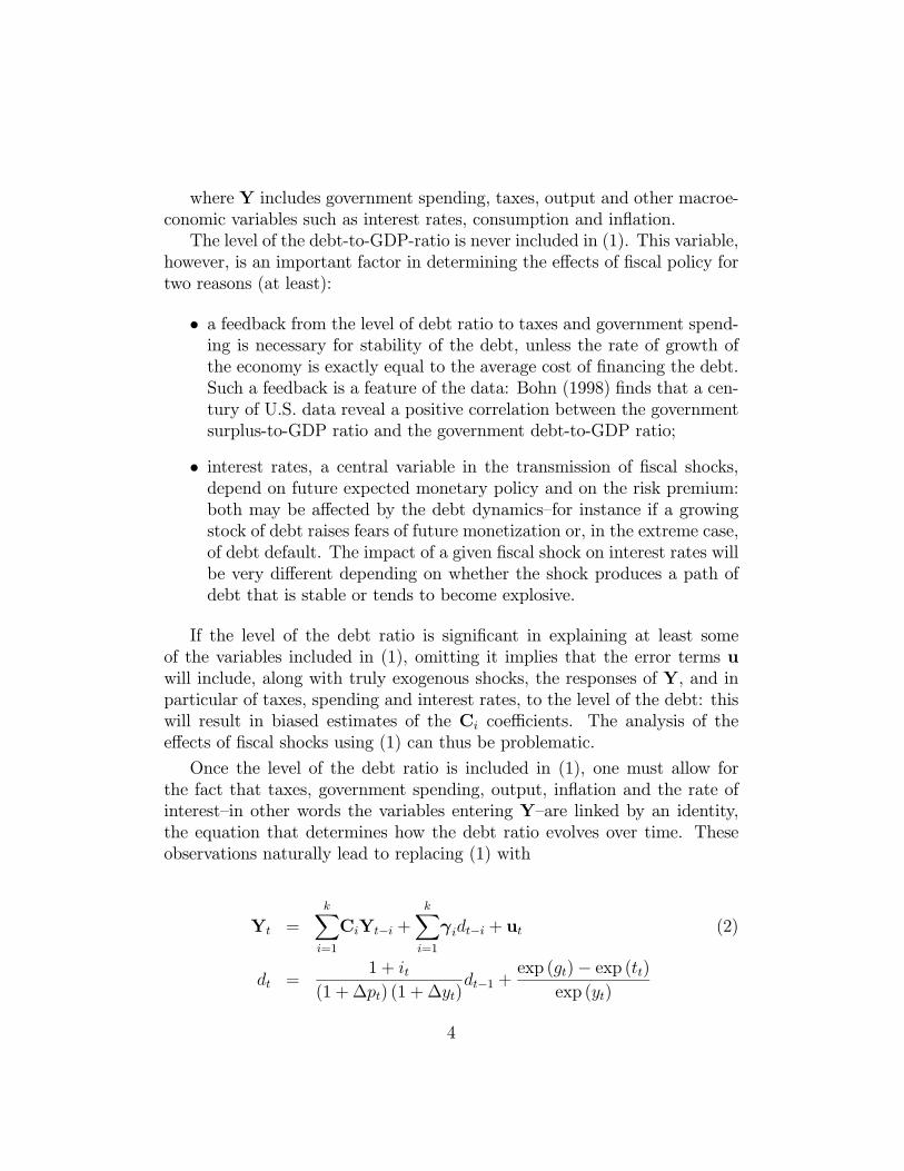
where Y includes government spending, taxes, output and other macroe-conomic variables such as interest rates, consumption and inflation.The level of the debt-to-GDP-ratio is never included in (1). This variable,

however, is an important factor in determining the effects of fiscal policy fortwo reasons (at least):

• a feedback from the level of debt ratio to taxes and government spend-ing is necessary for stability of the debt, unless the rate of growth ofthe economy is exactly equal to the average cost of financing the debt.Such a feedback is a feature of the data: Bohn (1998) finds that a cen-tury of U.S. data reveal a positive correlation between the governmentsurplus-to-GDP ratio and the government debt-to-GDP ratio;

• interest rates, a central variable in the transmission of fiscal shocks,depend on future expected monetary policy and on the risk premium:both may be affected by the debt dynamics—for instance if a growingstock of debt raises fears of future monetization or, in the extreme case,of debt default. The impact of a given fiscal shock on interest rates willbe very different depending on whether the shock produces a path ofdebt that is stable or tends to become explosive.

If the level of the debt ratio is significant in explaining at least someof the variables included in (1), omitting it implies that the error terms uwill include, along with truly exogenous shocks, the responses of Y, and inparticular of taxes, spending and interest rates, to the level of the debt: thiswill result in biased estimates of the Ci coefficients. The analysis of theeffects of fiscal shocks using (1) can thus be problematic.

Once the level of the debt ratio is included in (1), one must allow forthe fact that taxes, government spending, output, inflation and the rate ofinterest—in other words the variables entering Y—are linked by an identity,the equation that determines how the debt ratio evolves over time. Theseobservations naturally lead to replacing (1) with

Yt =kXi=1

CiYt−i +kXi=1

γidt−i + ut (2)

dt =1 + it

(1 +∆pt) (1 +∆yt)dt−1 +

exp (gt)− exp (tt)exp (yt)

4

where Y0t =

£gt tt yt ∆pt it

¤. d is the debt-to-GDP ratio, i is the

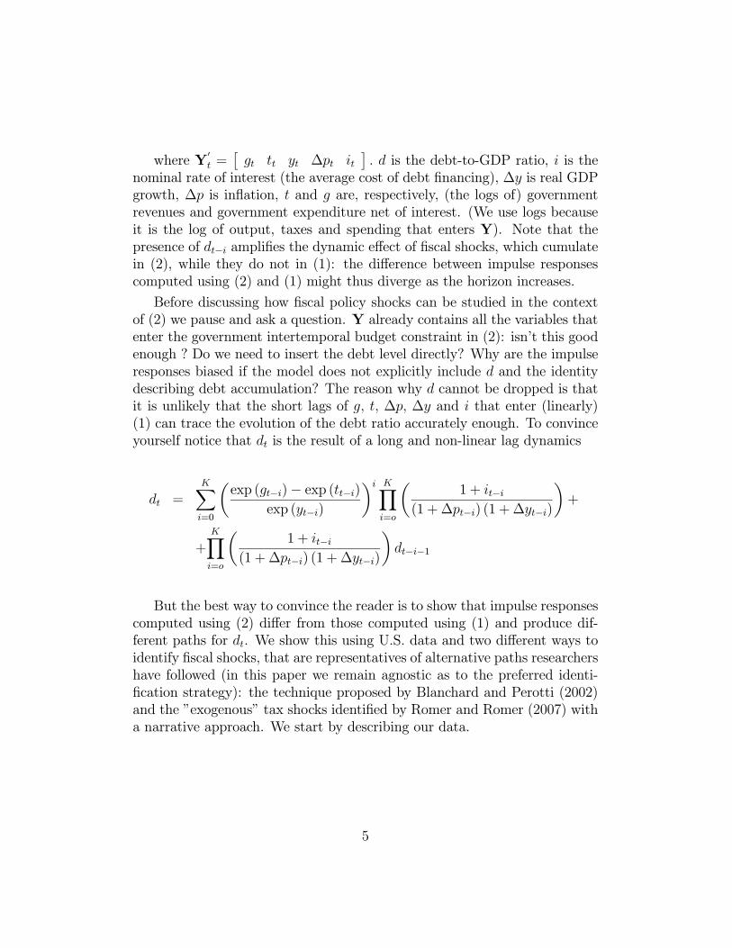
nominal rate of interest (the average cost of debt financing), ∆y is real GDPgrowth, ∆p is inflation, t and g are, respectively, (the logs of) governmentrevenues and government expenditure net of interest. (We use logs becauseit is the log of output, taxes and spending that enters Y). Note that thepresence of dt−i amplifies the dynamic effect of fiscal shocks, which cumulatein (2), while they do not in (1): the difference between impulse responsescomputed using (2) and (1) might thus diverge as the horizon increases.

Before discussing how fiscal policy shocks can be studied in the contextof (2) we pause and ask a question. Y already contains all the variables thatenter the government intertemporal budget constraint in (2): isn’t this goodenough ? Do we need to insert the debt level directly? Why are the impulseresponses biased if the model does not explicitly include d and the identitydescribing debt accumulation? The reason why d cannot be dropped is thatit is unlikely that the short lags of g, t, ∆p, ∆y and i that enter (linearly)(1) can trace the evolution of the debt ratio accurately enough. To convinceyourself notice that dt is the result of a long and non-linear lag dynamics

dt =KXi=0

µexp (gt−i)− exp (tt−i)

exp (yt−i)

¶i KYi=o

µ1 + it−i

(1 +∆pt−i) (1 +∆yt−i)

¶+

+KYi=o

µ1 + it−i

(1 +∆pt−i) (1 +∆yt−i)

¶dt−i−1

But the best way to convince the reader is to show that impulse responsescomputed using (2) differ from those computed using (1) and produce dif-ferent paths for dt. We show this using U.S. data and two different ways toidentify fiscal shocks, that are representatives of alternative paths researchershave followed (in this paper we remain agnostic as to the preferred identi-fication strategy): the technique proposed by Blanchard and Perotti (2002)and the ”exogenous” tax shocks identified by Romer and Romer (2007) witha narrative approach. We start by describing our data.

5

3 The data

We begin using quarterly data for the U.S. economy since 1960:1, the sampleanalyzed in Blanchard and Perotti (2002) and extended to 2005:4 in Perotti(2007). Our approach requires that the debt-dynamics equation in (2) tracksthe path of dt accurately: we thus need to define the variables in this equationwith some care.

The source for the different components of the budget deficit and for allmacroeconomic variables are the NIPA accounts (available on the Bureau ofEconomic Analysis website, downloaded on December 7th 2006). yt is (thelog of) real GDP per capita, ∆pt is the log difference of the GDP defla-tor. Data for the stock of U.S. public debt and for population are from theFRED database (available on the Federal Reserve of St.Louis website,alsodownloaded on December 7th 2006). Our measure for gt is (the log of)real per capita primary government expenditure: nominal expenditure is ob-tained subtracting from total Federal Government Current Expenditure (line39, NIPA Table 3.2 ) net interest payments at annual rates (obtained as thedifference between line 28 and line 13 on the same table). Real per capitaexpenditure is then obtained by dividing the nominal variable by populationtimes the GDP chain deflator. Our measure for tt is (the log of) real percapita government receipts at annual rates (the nominal variable is reportedon line 36 of the same NIPA Table).

The average cost servicing the debt, it, is obtained by dividing net interestpayments by the federal government debt held by the public (FYGFDPUNin the Fred database) at time t − 1. The federal government debt heldby the public is smaller than the gross federal debt, which is the broadestdefinition of the U.S. public debt. However, not all gross debt representspast borrowing in the credit markets since a portion of the gross federaldebt is held by trust funds—primarily the Social Security Trust Fund, butalso other funds: the Trust Fund for Unemployment Insurance, the HighwayTrust Fund, the pension fund of federal employees, etc.. The assets held bythese funds consist of non-marketable debt.1 We thus exclude it from ourdefinition of federal public debt.

Figure 1 reports, starting in 1970:1 (the first quarter for which the debtdata are available in FRED), this measure of the debt held by the public as

1Cashell (2006) notes that ”this debt exists only as a book-keeping entry, and does notreflect past borrowing in credit markets.”

6

a fraction of GDP (this is the dotted line). We have checked the accuracyof the debt dynamics equation in (2) simulating it forward from 1970:1 (thisis the continuous line in Figure 1). The simulated series is virtually super-imposed to the actual one: the small differences are due to approximationerrors in computing inflation and growth rates as logarithmic differences, andto the fact that the simulated series are obtained by using seasonally adjustedmeasures of expenditures and revenues. Based on this evidence we have usedthe debt dynamics equation to extend dt back to 1950:1. (A quarterly seriesfor dt extending back to 1950:1 will become necessary when we compare ourresults with those in Romer and Romer (2007) whose sample starts just afterWorld War II.) Figure 1 shows that this series tracks the annual debt levelaccurately, at least up to the early 1950’s. 2

4 Fiscal shocks identified from SVAR’s

We start by comparing (2) with the Structural VAR (SVAR) estimated inBlanchard and Perotti (2002) and extended in Perotti (2007) (B&P in whatfollows).

SVAR’s identify fiscal shocks imposing restrictions that allow the twostructural fiscal shocks in (1) to be recovered from the reduced form resid-uals, u. The innovations in the reduced form equations for taxes and gov-ernment spending, ugt and utt, contain three terms: (i) the response of taxesand government spending to fluctuations in macroeconomic variables, suchas output and inflation, that is implied by the presence of automatic stabiliz-ers; (ii) the discretionary response of fiscal policy to news in macro variablesand (iii) truly exogenous shifts in taxes and spending, the shocks we wish toidentify. B&P exploit the fact that it typically takes longer than a quarterfor discretionary fiscal policy to respond to news in macroeconomic variables:at quarterly frequency the contemporaneous discretionary response of fiscalpolicy to macroeconomic data can thus be assumed to be zero. To identifythe component of ugt and utt which corresponds to automatic stabilizers theyuse institutional information on the elasticities of tax revenues and govern-ment spending to macroeconomic variables. They thus identify the structural

2We are unable to build the debt series back to 1947:1, the start of the Romer andRomer sample, because data for total governemnt spending, needed to buld the debt series,are available on a consistent basis only from 1950:1.

7

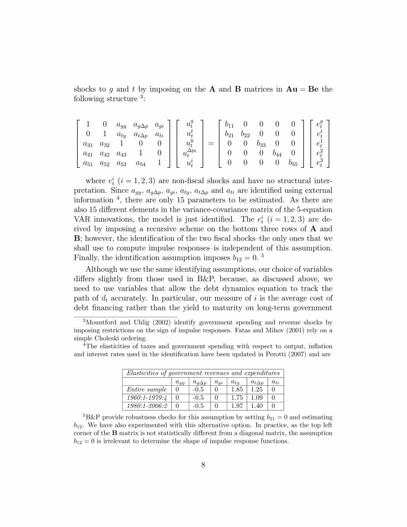
shocks to g and t by imposing on the A and B matrices in Au = Be thefollowing structure 3:

⎡⎢⎢⎢⎢⎣1 0 agy ag∆p agi0 1 aty at∆p atia31 a32 1 0 0a41 a42 a43 1 0a51 a52 a53 a54 1

⎤⎥⎥⎥⎥⎦⎡⎢⎢⎢⎢⎣

ugtuttuytu∆ptt

uit

⎤⎥⎥⎥⎥⎦ =⎡⎢⎢⎢⎢⎣

b11 0 0 0 0b21 b22 0 0 00 0 b33 0 00 0 0 b44 00 0 0 0 b55

⎤⎥⎥⎥⎥⎦⎡⎢⎢⎢⎢⎣

egtette1te2te3t

⎤⎥⎥⎥⎥⎦where eit (i = 1, 2, 3) are non-fiscal shocks and have no structural inter-

pretation. Since agy, ag∆p, agi, aty, at∆p and ati are identified using externalinformation 4, there are only 15 parameters to be estimated. As there arealso 15 different elements in the variance-covariance matrix of the 5-equationVAR innovations, the model is just identified. The eit (i = 1, 2, 3) are de-rived by imposing a recursive scheme on the bottom three rows of A andB; however, the identification of the two fiscal shocks—the only ones that weshall use to compute impulse responses—is independent of this assumption.Finally, the identification assumption imposes b12 = 0.

5

Although we use the same identifying assumptions, our choice of variablesdiffers slightly from those used in B&P, because, as discussed above, weneed to use variables that allow the debt dynamics equation to track thepath of dt accurately. In particular, our measure of i is the average cost ofdebt financing rather than the yield to maturity on long-term government

3Mountford and Uhlig (2002) identify government spending and revenue shocks byimposing restrictions on the sign of impulse responses. Fatas and Mihov (2001) rely on asimple Choleski ordering.

4The elasticities of taxes and government spending with respect to output, inflationand interest rates used in the identification have been updated in Perotti (2007) and are

Elasticities of government revenues and expendituresagy ag∆p agi aty at∆p ati

Entire sample 0 -0.5 0 1.85 1.25 01960:1-1979:4 0 -0.5 0 1.75 1.09 01980:1-2006:2 0 -0.5 0 1.97 1.40 0

5B&P provide robustness checks for this assumption by setting b21 = 0 and estimatingb12. We have also experimented with this alternative option. In practice, as the top leftcorner of the B matrix is not statistically different from a diagonal matrix, the assumptionb12 = 0 is irrelevant to determine the shape of impulse response functions.

8

bonds used in B&P. Our definitions of g and t are also slightly different: wefollow the NIPA definitions by considering net transfers as part of governmentexpenditure, rather than subtracting them from taxes.

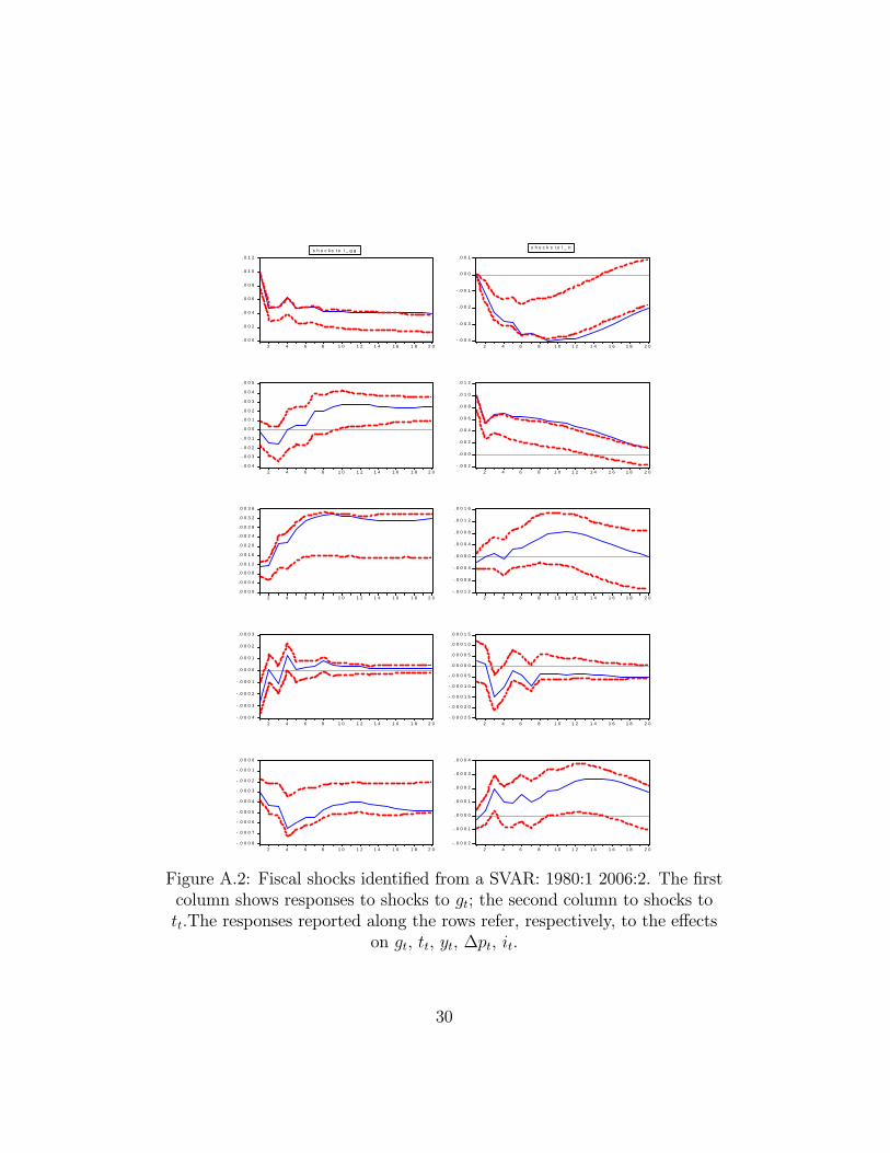
To check that our slight differences in data definitions do not change theresults we have first estimated (1) as in B&P. Following Perotti (2007) whofinds differences in the impulse response functions before and after 1980, thesample is split in two sub-samples 1960:1-1979:4 and 1980:1-2006:2. Theimpulse responses are reported in Figures A1 and A2 in the Appendix andare consistent with those reported in B&P. In particular:

• an (exogenous) increase in public expenditure has an expansionary ef-fect on output, while an (exogenous) increase in revenues is contrac-tionary. The impact of fiscal policy weakens in the second sub-sample,in particular the effects of tax shocks become insignificant;

• after 1980 fiscal shocks become less persistent;• the effect of fiscal shocks on interest rates is insignificant in the first sub-sample; it is small, significant but counterintuitive in the second sub-sample when an increase in public spending lowers the cost of servicingthe debt;

• fiscal shocks have consistently no significant effect on inflation.

4.1 The debt dynamics implied by a standard SVAR

To assess the importance of omitting d, we start with a simple exercise. Afterhaving estimated the parametersCi in (1) we use the identity which describesdebt accumulation to simulate the system out-sample for 80 quarters startingfrom the conditions prevailing in the last observation of the estimation period.The path for dt so constructed reveals the steady state properties of theestimated empirical model.

When (1) is estimated over the first sub-sample (1960:1-1979:4) the sim-ulated out-of-sample path for dt diverges (Figure 2). When (1) is estimatedover the second sub-sample (1980:1-2006:2) the simulated debt ratio tends,eventually, to fall below zero.

This exercise naturally raises a number of questions:

9

• does the apparent instability depend on the underlying behavior of thegovernment, or is it simply the result of a mis-specified model? Debtstabilization requires that the primary budget surplus reacts to theaccumulation of debt, but such a reaction—if it were in the data—wouldnot be captured by (1). Hence the simulated path may very well bethe result of a mis-specification of the empirical model rather than adescription of the actual behavior of the government;

• it is obviously difficult to interpret impulse response functions whenthey are computed along unstable paths for the debt ratio, as theywould eventually diverge. An unstable dynamics becomes particularlyproblematic when the effects of fiscal shocks are computed over rela-tively long horizons, or when identification is obtained imposing longrun restrictions on the shape of impulse responses. This is not the casein the B&P identification, that is achieved imposing restrictions on thesimultaneous effects of fiscal policy shocks. However, the interpreta-tion of the responses to shocks along an unstable debt path remainsproblematic;

• impulse response functions appear to differ over the two sub-samples.Does this depend on the different dynamics for the debt-to-GDP ratioimplied by the SVAR estimated over the two sub-periods? In particu-lar (1) often produces a puzzling response of interest rates to a fiscalshock. Consider for example the response to an expansionary fiscalshock over the first sub-sample. The path of the debt ratio eventuallybecomes explosive: how can this be reconciled with the evidence thatthe estimated response of it is small and insignificant?

• impulse responses are often used to discriminate between competingDSGE models, or to provide evidence on the stylized facts to include intheoretical models used for policy analysis. It is obviously impossible tocompare the empirical evidence from a model that delivers an explosivepath for the debt, with the paths of variables generated by forwardlooking models, since such models do not have a solution when thedebt dynamics is unstable.

We now turn to the model described in (2).

10

4.2 Estimating the effects of fiscal shocks in a SVARwith debt dynamics

The identification problem does not change when the debt level is includedin the model. Since we treat the debt-deficit relationship as an identity,the number of shocks remains the same, so that the identification assump-tions discussed in the previous section remain valid. Also, since there areno parameters to be estimated in the debt-dynamics equation, (2) can beestimated excluding that equation. The identified system is therefore

Yt =kXi=1

CiYt−i +kXi=1

γidt−i +A−1Bet (3)

dt =1 + it

(1 +∆pt) (1 +∆yt)dt−1 +

exp (gt)− exp (tt)exp (yt)

Table 1 reports the estimated coefficients of the first and the second lagsof dt in the five equations (taxes, spending, output, inflation and the cost ofdebt service) in the two sub-samples.

[INSERT TABLE 1 HERE]

In all equations the restriction that the two coefficients are of equal mag-nitude and of opposite sign cannot be rejected, suggesting that the five vari-ables respond to the lagged change in the debt ratio. The last two rows inthe Table report the coefficients (and their standard errors) when this re-striction is imposed. For instance, government spending is reduced when thelagged change in the debt ratio is positive. (dt−1 − dt−2) measures the gapbetween the actual primary surplus (as a fraction of GDP) and the surplusthat would stabilize d: the magnitude of the coefficient indicates that thegap between the surplus that would stabilize the debt ratio and the actualsurplus acts as an error correction mechanism in the fiscal reaction function:current expenditures are decreased when last period’s primary surplus wasbelow the level that would have kept the debt ratio stable.

The response of gt to a change in the debt-ratio is significant after 1980,not before. Taxes do not respond significantly to a change in the debt ratio,however the difference between the point estimates between the two sub-periods is close to being significant and the response is stabilizing only after1980. The average interest cost of the debt also depends on the gap between

11

the actual surplus and the debt stabilizing surplus. This result is particularlystrong in the second sub-sample. Finally, the direct effect of lags in dt oninflation and output is never significant in any of the samples.

Summing up. Before 1980 U.S. fiscal policy does not seem to have beenaimed at stabilizing the debt-to-GDP ratio: this probably reflects the willof the fiscal authorities to reduce the debt ratio from the high initial levelinherited after World War II. Only after 1980 does fiscal policy become sta-bilizing. Using the coefficients estimated up to 1980 to simulate the effects ofa fiscal policy shock is thus inappropriate, since such a shock would put thedebt ratio on a diverging path, while the coefficients have been estimated ona sample characterized by a decreasing debt ratio.

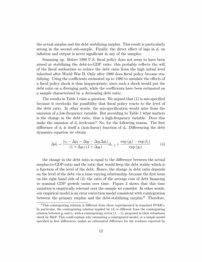
The results in Table 1 raise a question. We argued that (1) is mis-specifiedbecause it overlooks the possibility that fiscal policy reacts to the level ofthe debt ratio. In other words, the mis-specification would arise from theomission of a low-frequency variable. But according to Table 1 what mattersis the change in the debt ratio, thus a high-frequency variable. Does thismake the omission of dt irrelevant? No, for the following reason. The firstdifference of dt is itself a (non-linear) function of dt. Differencing the debtdynamics equation we obtain

∆dt =(it −∆pt −∆yt −∆yt∆pt)

(1 +∆pt) (1 +∆yt)dt−1 +

exp (gt)− exp (tt)exp (yt)

(4)

the change in the debt ratio is equal to the difference between the actualsurplus-to-GDP-ratio and the ratio that would keep the debt stable—which isa function of the level of the debt. Hence, the change in debt ratio dependson the level of the debt via a time-varying relationship—because the first termon the right hand side of (4)—the ratio of the average cost of debt financingto nominal GDP growth—varies over time. Figure 3 shows that this timevariation is empirically relevant over the sample we consider. In other words,our empirical model is an error correction model consistent with cointegrationbetween the primary surplus and the debt-stabilizing surplus.6 Therefore,

6This cointegrating relation is different from those experimented in standard SVAR’s.In particular, the cointegrating relation implied by (4) is different from the cointegratingrelation between gt and tt, with a cointegrating vector (1, −1), proposed in their robustnesscheck by B&P. This could explain why estimating a cointegrated model, or a simple modelspecified in first differences, makes no substantial difference for the evidence reported by

12

including the change in d in a VAR is virtually equivalent to augmenting theVAR with a time-varying function of the level of the debt-to-GDP ratio, thatis indeed a slow moving variable7.

Computing impulse responses

The presence of the intertemporal budget constraint makes computing theresponses of the variables in Yt to innovations in et different from computingimpulse responses in a standard VAR. Impulse responses comparable to thoseobtained from the traditional moving average representation of a VAR canbe constructed going through the following steps:

• generate a baseline simulation for all variables by solving (3) dynam-ically forward (this requires setting to zero all shocks for a number ofperiods equal to the horizon up to which impulse responses are needed),

• generate an alternative simulation for all variables by setting to one—just for the first period of the simulation—the structural shock of in-terest, and then solve dynamically forward the model up to the samehorizon used in the baseline simulation,

• compute impulse responses to the structural shocks as the differencebetween the simulated values in the two steps above. (Note that thesesteps, if applied to a standard VAR, would produce standard impulseresponses. In our case they produce impulse responses that allow forboth the feedback from dt−i to Yt and for the debt dynamics),

• compute confidence intervals.8

B&P. Of course, if the debt stabilizing surplus were stationary, the data would support—upto a logarithmic transformation—the cointegrating vector in B&P, but the long-run solutionof their cointegrating system would still be different from the one implied by a system inwhich there is tight relation between the actual surplus and the debt stabilizing surplus.The cointegrating relation implied by (4) is also different from the error correction modelproposed in Bohn (1988): Bohn includes the level of the debt ratio in the fiscal reactionfunction but does so without allowing for the time variation of the coefficient multiplyingthe debt level.

7As a robustness check we have re-run our SVAR augmenting it with the debt stabi-lizing surplus-to-GDP ratio lagged once and twice. The coefficients on the two lags whereequaly signed and their sum was not statistically different from the coefficient on the firstdifference of d, our proposed model.

8Bootstrapping requires saving the residuals from the estimated VAR and then iterating

13

We now turn to the results.

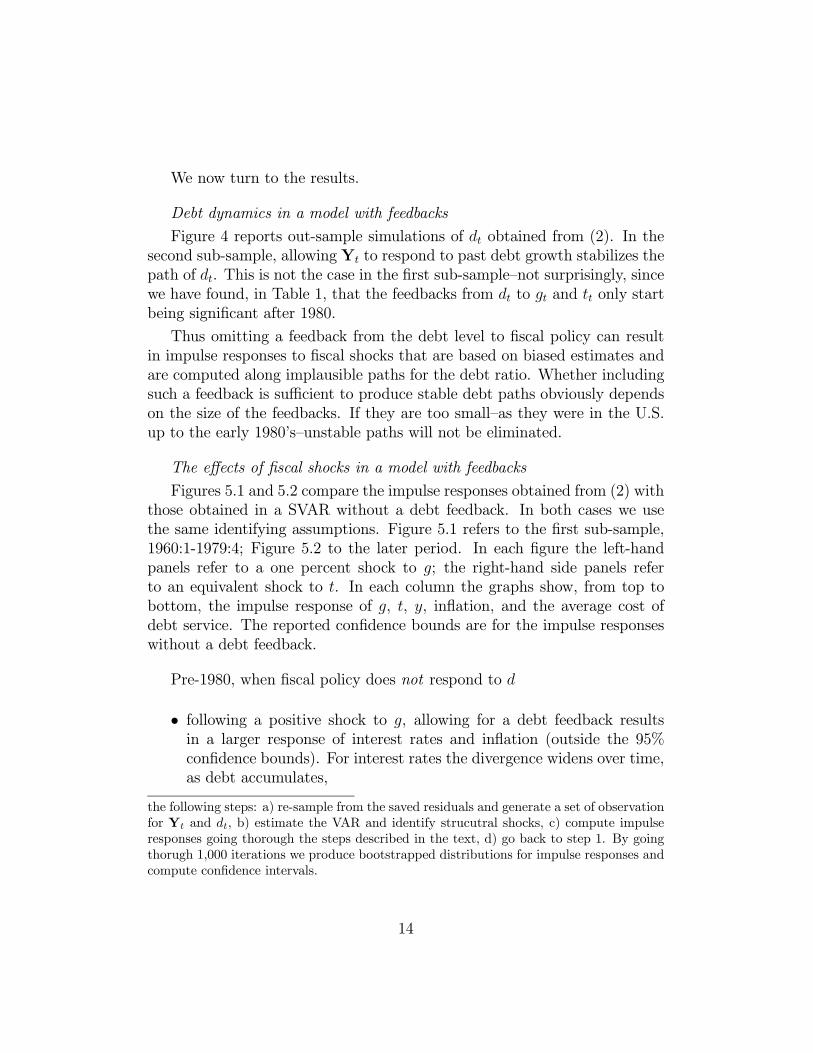
Debt dynamics in a model with feedbacks

Figure 4 reports out-sample simulations of dt obtained from (2). In thesecond sub-sample, allowing Yt to respond to past debt growth stabilizes thepath of dt. This is not the case in the first sub-sample—not surprisingly, sincewe have found, in Table 1, that the feedbacks from dt to gt and tt only startbeing significant after 1980.

Thus omitting a feedback from the debt level to fiscal policy can resultin impulse responses to fiscal shocks that are based on biased estimates andare computed along implausible paths for the debt ratio. Whether includingsuch a feedback is sufficient to produce stable debt paths obviously dependson the size of the feedbacks. If they are too small—as they were in the U.S.up to the early 1980’s—unstable paths will not be eliminated.

The effects of fiscal shocks in a model with feedbacks

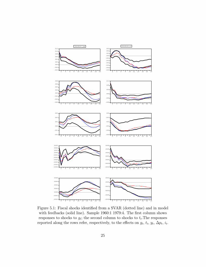
Figures 5.1 and 5.2 compare the impulse responses obtained from (2) withthose obtained in a SVAR without a debt feedback. In both cases we usethe same identifying assumptions. Figure 5.1 refers to the first sub-sample,1960:1-1979:4; Figure 5.2 to the later period. In each figure the left-handpanels refer to a one percent shock to g; the right-hand side panels referto an equivalent shock to t. In each column the graphs show, from top tobottom, the impulse response of g, t, y, inflation, and the average cost ofdebt service. The reported confidence bounds are for the impulse responseswithout a debt feedback.

Pre-1980, when fiscal policy does not respond to d

• following a positive shock to g, allowing for a debt feedback resultsin a larger response of interest rates and inflation (outside the 95%confidence bounds). For interest rates the divergence widens over time,as debt accumulates,

the following steps: a) re-sample from the saved residuals and generate a set of observationfor Yt and dt, b) estimate the VAR and identify strucutral shocks, c) compute impulseresponses going thorough the steps described in the text, d) go back to step 1. By goingthorugh 1,000 iterations we produce bootstrapped distributions for impulse responses andcompute confidence intervals.

14

• following a positive shock to t, interest rates fall more in the modelwith feedbacks and the difference also widens over time,

• the output effects of shocks to g and t are larger in the model with adebt feedback.

Post-1980, when fiscal policy is stabilizing

• following positive t shock output rises. In the model without a debtfeedback the effect on output of a shock to t is never statistically signif-icant. The larger increase in output in the model with a debt feedbackis partly explained by the response of spending to a tax shock: g ini-tially falls as taxes rise, but eventually it rises—a feature of the stabilityof fiscal policy in this sub-sample,

• g shocks are less persistent in the model with a feedback and t respondsoffsetting g shocks—again a feature of stability,

• the response of interest rates to a positive g shock is still negative atthe beginning, but rises over time in the presence of a feedback,

• following a shock to t interest rates rise more in the presence of afeedback, mirroring the larger increase in y.

Table 2 complements the result in Figures 5 by computing the cumulativeresponse of interest rates and output to a fiscal shock over three horizons, (4,12 and 20 quarters) and comparing them with the responses in the absenceof a debt feedback. The effect of a 1% g shock on interest rates, cumulatedover 20 quarters, in the first sub-sample, is 0.118 in the model with feed-back, 0.032 without: the larger reaction of interest rates to a fiscal shock isconsistent with the finding that in the first sub-sample fiscal policy is notstabilizing. This is confirmed by the observation that the differences in thecumulated responses of interest rates vanish in the second sub-sample wherefiscal policy is stabilizing. The expansionary effect of a tax increase in thesecond-subsample is confirmed by the cumulated responses. Following a 1%increase in taxes output rises (over a 20 quarters horizon) by 0.288 in themodel with feedback, as opposed to 0.170 in the model without a feedback.

[INSERT TABLE 2 HERE]

15

5 Fiscal shocks identified from the narrative

record

Romer and Romer (2007) (R&R in what follows) use the U.S. narrativerecord—presidential speeches, executive-branch documents, and Congressionalreports—to classify the size (defined as the estimated revenue effect of a newtax bill), timing, and principal motivation for all major postwar tax policyactions.9 They then identify, among all documented tax actions, those thatcould be classified as ”exogenous”, as opposed to those that were counter-cyclical, i.e. motivated by a desire to return output growth to normal. Ex-ogenous tax changes are further divided into two groups: those that appearto be motivated by a desire to raise the potential growth rate of the econ-omy, and those aimed at reducing a budget deficit inherited from previousadministrations.

Since 1947 U.S. Federal laws changed taxes in 82 quarters. A numberof these quarters had tax changes of multiple types. Among the 104 sepa-rate quarterly tax changes identified, 65 are classified as exogenous. In thisSection we use these 65 tax changes (the R&R exogenous tax shocks) andask what difference it makes if the debt channel is, or is not, included in thetransmission mechanism.

R&R estimate the impact of tax shocks on output using a single-equationapproach:

∆yt = β0 +12Xi=1

βi∆T ex

t−1Yt−1

+kX

j=1

γjZt−j + et (5)

where ∆yt is real quarterly output growth,∆T ext−1Yt−1

are the tax shocks,

measured as a percent of nominal GDP, and Zt−j are controls (lags of ∆yt,monetary policy shocks, government spending, oil prices). The Z 0s are as-sumed to be exogenous, and in particular unaffected by the tax shocks, noteven with a lag. The R&R exercise should thus be interpreted as asking thefollowing (hypothetical) question: Assume that the transmission mechanism

9Early attempts at applying to fiscal policy the methodology proposed by Romer andRomer (1989) to identify monetary policy shocks were Edelberg, Eichenbaum and Fisher(1999), Burnside, Eichenbaum and Fisher (2004), Ramey (2006). These papers used adummy variable which identifies characterizes episodes of significant and exogenous in-creases in government spending (typically wars).

16

of tax shocks is shut down and that such shocks only affect output directly,rather than, for instance, also via their effect on interest rates. What is theireffect on output under this hypothesis? R&R find that ”exogenous” tax in-creases have a larger negative effect on output than countercyclical tax hikes.Among the exogenous tax increases, those motivated by the aim to rein in abudget deficit are less contractionary.—in fact the negative impact on outputis statistically insignificant.

To estimate the effects of the R&R tax shocks when fiscal policy is allowedto respond to the level of the debt we first need to embed these shocks in amodel that doesn’t shut down the transmission mechanism. We do this usingthe R&R shocks in the two VAR’s analyzed above: (1) and (2).10 Therefore,we estimate the following two models:

Yt =kXi=1

CiYt−i + δi∆T ex

t

Tt+ ut (6)

Yt =kXi=1

CiYt−i +kXi=1

γidt−i + δi∆T ex

t

Tt+ ut (7)

dt =1 + it

(1 +∆pt) (1 +∆yt)dt−1 +

exp (gt)− exp (tt)exp (yt)

where the variables in Y are, as before, taxes, government spending,output, inflation and interest rates.

Including the R&R tax shocks in a VAR is a natural way of computingthe dynamic response of macro variables to shocks identified outside the VARbecause what matters are the impulse responses generated by the differentshocks, not the correlation of the shocks themselves. 11 The R&R shocks arevalid shocks to taxes because we find that they are uncorrelated with all lagsof the variables included in the VAR’s and are significant only in the equation

10R&R scale their shocks by the level of GDP. We scale them by taxes to allow directcomparability of the effects of these shocks with those identified in a SVAR. In a SVAR taxshocks are extracted from a specification in the logarithms of the levels of real variables.Innovations thus have the dimension of a percentage change in taxes. A one per centchange in taxes is much smaller than a one per cent shock in the tax-to-GDP ratio. There-scaling affects the size of the effects but not the shape of the impulse responses.11VAR’s have been used to compute impulse responses to shocks identified outside the

VAR in the analysis of the effects of monetary shocks in Bagliano and Favero (1999).

17

for t. Thus they satisfy the properties that exogenous shocks identified in astructural VAR should fulfill.

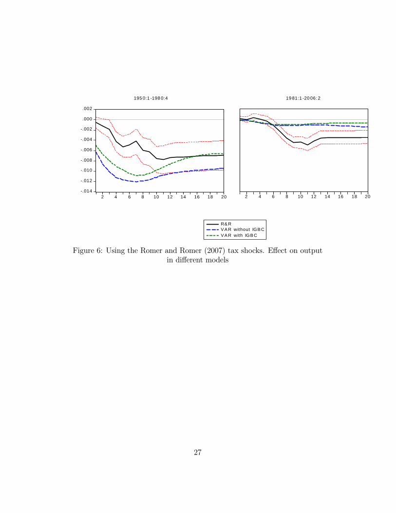
Figure 6 shows the impulse response of output to an exogenous R&R taxshock equivalent to 1% of taxes. Impulse responses are computed usingthree different models:

• (5), the equation estimated by R&R where we have replaced ∆T ext−1Yt−1

with∆T ext−1Tt−1

,

• (6), a VAR that excludes a debt feedback• (7), a model that allows the variables in the VAR to respond to thelevel of the debt.

The R&R shocks start in 1947, while our data, for the reasons noted infootnote 2, only start in 1950:1: we thus miss the exogenous shocks thatoccurred between January 1947 and December 1949. As in the previousSection we split the sample in two parts: 1950:1-1979:4 and 1980:1-2006:2.

The effects on output of the exogenous R&R tax shocks are quite differentin the two sub-samples and depending on the model they are embedded in.In the first sub-sample (1950:1-1979:4) the contractionary. effect of a taxhike is larger when Z is endogenized in a model that includes the level of thedebt and the government intertemporal budget constraint. This probablyhappens because—as documented in the previous Section—debt stabilizationdoes not appear to have been a concern for the U.S. fiscal authorities in thefirst part of the sample. A tax increase thus did not call for a compensatingchange in the budget. Fiscal shocks could cumulate over time amplifying theeffect on output of an initial shock. This may explain why tax hikes havelarger effects in the models that allow the variables in Z to respond to theshock.

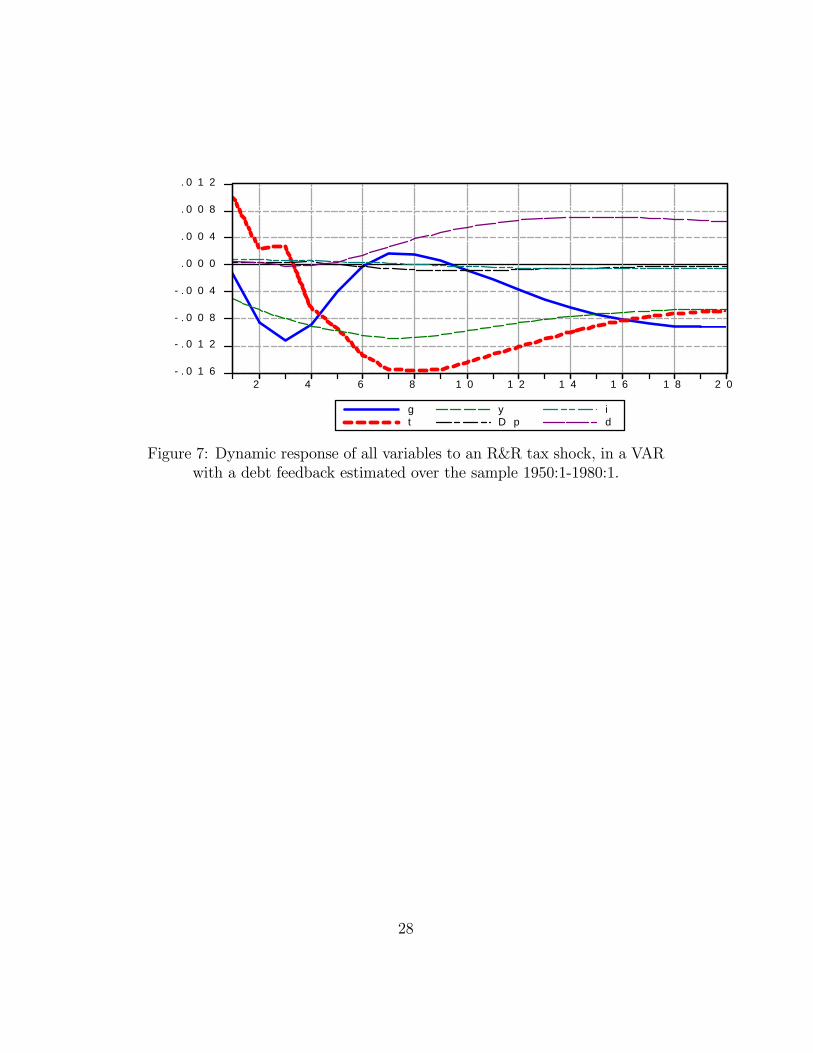
In the second sub-sample, when fiscal policy becomes stabilizing–-a pos-itive shock to taxes is compensated by a subsequent fiscal accommodation.This explains why, analyzing the effects of shocks in a model where Z is en-dogenous and fiscal policy responds to the debt level, produces much smalleroutput effects compared with the R&R single equation model. Figure 7shows that in fact, in the second sub-sample, an initial positive tax shockis accompanied by further tax changes in the opposite direction. Followingthe initial shock taxes fall: when this happens the effect on the budget is

18

compensated by increases in spending. These responses are not captured in(5) because the equation sets to zero the dynamic response of all variables,with the only exception of output growth, to tax shocks.

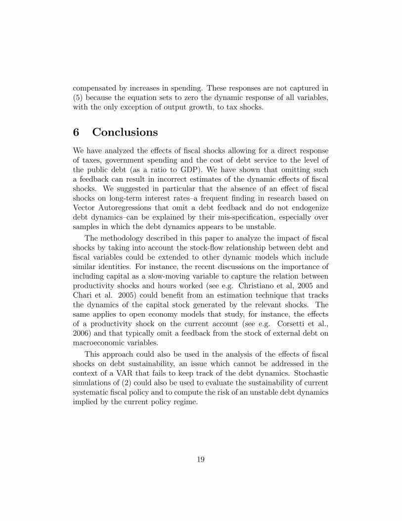
6 Conclusions

We have analyzed the effects of fiscal shocks allowing for a direct responseof taxes, government spending and the cost of debt service to the level ofthe public debt (as a ratio to GDP). We have shown that omitting sucha feedback can result in incorrect estimates of the dynamic effects of fiscalshocks. We suggested in particular that the absence of an effect of fiscalshocks on long-term interest rates—a frequent finding in research based onVector Autoregressions that omit a debt feedback and do not endogenizedebt dynamics—can be explained by their mis-specification, especially oversamples in which the debt dynamics appears to be unstable.

The methodology described in this paper to analyze the impact of fiscalshocks by taking into account the stock-flow relationship between debt andfiscal variables could be extended to other dynamic models which includesimilar identities. For instance, the recent discussions on the importance ofincluding capital as a slow-moving variable to capture the relation betweenproductivity shocks and hours worked (see e.g. Christiano et al, 2005 andChari et al. 2005) could benefit from an estimation technique that tracksthe dynamics of the capital stock generated by the relevant shocks. Thesame applies to open economy models that study, for instance, the effectsof a productivity shock on the current account (see e.g. Corsetti et al.,2006) and that typically omit a feedback from the stock of external debt onmacroeconomic variables.

This approach could also be used in the analysis of the effects of fiscalshocks on debt sustainability, an issue which cannot be addressed in thecontext of a VAR that fails to keep track of the debt dynamics. Stochasticsimulations of (2) could also be used to evaluate the sustainability of currentsystematic fiscal policy and to compute the risk of an unstable debt dynamicsimplied by the current policy regime.

19

7 References

Bagliano, Fabio and C. Favero [1999]: ”Information from financial mar-kets and VAR measures of monetary policy”, The European EconomicReview, 43, 825-837.

Blanchard, Olivier and R. Perotti [2002]: ”An Empirical Characterizationof the Dynamic Effects of Changes in Government Spending and Taxeson Output”, Quarterly Journal of Economics

Bohn, Henning [1998]: ”The Behaviour of U.S. public debt and deficits”,Quarterly Journal of Economics, 113, 949-963.

Burnside, Craig, M. Eichenbaum and J.D.M. Fisher [2003]: “Fiscal Shocksand Their Consequences”, NBER Working Paper No 9772

Cashell, Brian W. [2006]: ”The Federal Government Debt: its size andeconomic significance” CRS Report for Congress.

Chari V.V., P.J. Kehoe and E.R. McGrattan [2005]: ”A Critique of Struc-tural VARs Using Business Cycle Theory”, Federal Reserve Bank ofMinneapolis Research Department Staff Report 364

Christiano, Lawrence J., M.Eichenbaum and R.Vigfusson [2005]: ”AssessingStructural VARs”, mimeo

Corsetti, Giancarlo, L. Dedola and S. Leduc [2006]: ”Productivity, ExternalBalance and Exchange Rates: Evidence on the Transmission Mecha-nism Among G7 Countries, forthcoming

Edelberg, Wendy, M. Eichenbaum and J. D.M. Fisher [1999]: ”Understand-ing the Effects of a Shock to Government Purchases”, Review of Eco-nomics Dynamics, pp.166-206, 41

Fatas, Antonio and I. Mihov [2001]: ”The Effects of Fiscal Policy on Con-sumption and Employment: Theory and Evidence”, mimeo, INSEAD

Giavazzi, Francesco, T. Jappelli and M. Pagano [2000]: ”Searching for Non-Linear Effects of Fiscal Policy: Evidence from Industrial and Develop-ing Countries”, European Economic Review, 44, no. 7, June.

20

Mountford, Andrew and H. Uhlig [2002]: ”What Are the Effcets of FiscalPolicy Shocks?” CEPR Discussion Paper 3338

Perotti, Roberto [2007]: “In Search of the Transmission Mechanism of Fiscalpolicy”; NBER Macroeconomic Annual, forthcoming

Ramey, Valerie [2006]: ”Identifying Government Spending Shocks: It’s Allin the Timing”, mimeo, July

Romer, Christina and David H. Romer [1989]: “Does Monetary Policy Mat-ter? A new test in the spirit of Friedman and Schwartz” in Blanchard,O. and S. Fischer, (eds.), NBER Macroeconomics Annual, Cambridge,MIT Press, 4, 121-170

Romer, Christina and David H. Romer [2007]: The Macroeconomic Effectsof Tax Changes: Estimates Based on a New Measure of Fiscal Shocks”,mimeo, March.

21

0 . 0

0 . 2

0 . 4

0 . 6

0 . 8

1 . 0

5 5 6 0 6 5 7 0 7 5 8 0 8 5 9 0 9 5 0 0 0 5

D Y D Y _ I

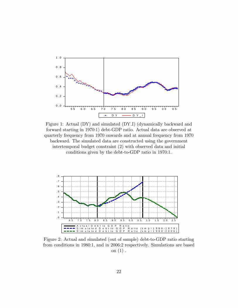
Figure 1: Actual (DY) and simulated (DY I) (dynamically backward andforward starting in 1970:1) debt-GDP ratio. Actual data are observed atquarterly frequency from 1970 onwards and at annual frequency from 1970backward. The simulated data are constructed using the governmentintertemporal budget constraint (2) with observed data and initial

conditions given by the debt-to-GDP ratio in 1970:1.

. 0

. 1

. 2

. 3

. 4

. 5

. 6

. 7

. 8

6 5 7 0 7 5 8 0 8 5 9 0 9 5 0 0 0 5 1 0 1 5 2 0 2 5

A c t u a l D e b t t o G D P R a t i oS i m u l a t e d D e b t t o G D P R a t i o ( s m p l 1 9 6 0 - 1 9 7 9 )S i m u l a t e d D e b t t o G D P R a t i o ( s m p l 1 9 8 0 - 2 0 0 6 )

Figure 2: Actual and simulated (out of sample) debt-to-GDP ratio startingfrom conditions in 1980:1, and in 2006:2 respectively. Simulations are based

on (1) .

22

- .0 5

.0 0

.0 5

.1 0

.1 5

.2 0

.2 5

6 0 6 5 7 0 7 5 8 0 8 5 9 0 9 5 0 0 0 5

a v e r a g e c o s t o f f i n a n c i n g th e d e b t ( a n n u a li z e d )q u a r te r l y n o m i n a l G D P g r o w th ( a n n u a li z e d )

Figure 3: Average cost of debt financing and quarterly (annualized)nominal GDP growth

0 .2

0 .3

0 .4

0 .5

0 .6

0 .7

0 .8

0 .9

1 .0

6 5 7 0 7 5 8 0 8 5 9 0 9 5 0 0 0 5 1 0 1 5 2 0 2 5

A c tu a l D e b t to G D P R a t i oS i m u l a te d D e b t to G D P R a t i o ( s m p l 1 9 6 0 - 1 9 7 9 )S i m u l a te d D e b t to G D P R a t i o ( s m p l 1 9 8 0 - 2 0 0 6 )

Figure 4: Actual and simulated out-of sample debt-GDP dynamics(starting from conditions in 1980:1, and in 2006:2 respectively).

Simulations are based on (2).

23

-. 0 0 4

-.0 0 2

.0 0 0

.0 0 2

.0 0 4

.0 0 6

.0 0 8

.0 1 0

.0 1 2

2 4 6 8 1 0 1 2 1 4 1 6 1 8 2 0-.0 0 6

-.0 0 5

-.0 0 4

-.0 0 3

-.0 0 2

-.0 0 1

.0 0 0

.0 0 1

.0 0 2

.0 0 3

2 4 6 8 1 0 1 2 1 4 1 6 1 8 2 0

-.0 0 6

-.0 0 4

-.0 0 2

.0 0 0

.0 0 2

.0 0 4

.0 0 6

.0 0 8

2 4 6 8 1 0 1 2 1 4 1 6 1 8 2 0-.0 0 8

-.0 0 4

.0 0 0

.0 0 4

.0 0 8

.0 1 2

2 4 6 8 1 0 1 2 1 4 1 6 1 8 2 0

-.0 0 2

-.0 0 1

.0 0 0

.0 0 1

.0 0 2

.0 0 3

2 4 6 8 1 0 1 2 1 4 1 6 1 8 2 0-.0 0 5

-.0 0 4

-.0 0 3

-.0 0 2

-.0 0 1

.0 0 0

2 4 6 8 1 0 1 2 1 4 1 6 1 8 2 0

-.0 0 0 6

-.0 0 0 5

-.0 0 0 4

-.0 0 0 3

-.0 0 0 2

-.0 0 0 1

.0 0 0 0

.0 0 0 1

.0 0 0 2

.0 0 0 3

2 4 6 8 1 0 1 2 1 4 1 6 1 8 2 0-.0 0 0 4

-.0 0 0 2

.0 0 0 0

.0 0 0 2

.0 0 0 4

.0 0 0 6

.0 0 0 8

2 4 6 8 1 0 1 2 1 4 1 6 1 8 2 0

-.0 0 0 4

-.0 0 0 2

.0 0 0 0

.0 0 0 2

.0 0 0 4

.0 0 0 6

.0 0 0 8

2 4 6 8 1 0 1 2 1 4 1 6 1 8 2 0-.0 0 0 8

-.0 0 0 6

-.0 0 0 4

-.0 0 0 2

.0 0 0 0

.0 0 0 2

2 4 6 8 1 0 1 2 1 4 1 6 1 8 2 0

s h o c ks t o l _ g g s h o c ks t o l _ t t

Figure 5.1: Fiscal shocks identified from a SVAR (dotted line) and in modelwith feedbacks (solid line). Sample 1960:1 1979:4. The first column showsresponses to shocks to gt; the second column to shocks to tt.The responsesreported along the rows refer, respectively, to the effects on gt, tt, yt, ∆pt, it.

25

. 0 0 0

. 0 0 2

. 0 0 4

. 0 0 6

. 0 0 8

. 0 1 0

. 0 1 2

2 4 6 8 1 0 1 2 1 4 1 6 1 8 2 0- . 0 0 5

- . 0 0 4

- . 0 0 3

- . 0 0 2

- . 0 0 1

. 0 0 0

. 0 0 1

. 0 0 2

. 0 0 3

2 4 6 8 1 0 1 2 1 4 1 6 1 8 2 0

- . 0 0 3

- . 0 0 2

- . 0 0 1

. 0 0 0

. 0 0 1

. 0 0 2

. 0 0 3

. 0 0 4

. 0 0 5

2 4 6 8 1 0 1 2 1 4 1 6 1 8 2 0- . 0 0 4

- . 0 0 2

. 0 0 0

. 0 0 2

. 0 0 4

. 0 0 6

. 0 0 8

. 0 1 0

. 0 1 2

2 4 6 8 1 0 1 2 1 4 1 6 1 8 2 0

. 0 0 0 0

. 0 0 0 5

. 0 0 1 0

. 0 0 1 5

. 0 0 2 0

. 0 0 2 5

. 0 0 3 0

. 0 0 3 5

2 4 6 8 1 0 1 2 1 4 1 6 1 8 2 0- . 0 0 1 5

- . 0 0 1 0

- . 0 0 0 5

. 0 0 0 0

. 0 0 0 5

. 0 0 1 0

. 0 0 1 5

2 4 6 8 1 0 1 2 1 4 1 6 1 8 2 0

- . 0 0 0 5

- . 0 0 0 4

- . 0 0 0 3

- . 0 0 0 2

- . 0 0 0 1

. 0 0 0 0

. 0 0 0 1

. 0 0 0 2

2 4 6 8 1 0 1 2 1 4 1 6 1 8 2 0- . 0 0 0 2 0

- . 0 0 0 1 6

- . 0 0 0 1 2

- . 0 0 0 0 8

- . 0 0 0 0 4

. 0 0 0 0 0

. 0 0 0 0 4

. 0 0 0 0 8

. 0 0 0 1 2

. 0 0 0 1 6

2 4 6 8 1 0 1 2 1 4 1 6 1 8 2 0

- . 0 0 0 9

- . 0 0 0 8

- . 0 0 0 7

- . 0 0 0 6

- . 0 0 0 5

- . 0 0 0 4

- . 0 0 0 3

- . 0 0 0 2

- . 0 0 0 1

. 0 0 0 0

2 4 6 8 1 0 1 2 1 4 1 6 1 8 2 0- . 0 0 0 2

- . 0 0 0 1

. 0 0 0 0

. 0 0 0 1

. 0 0 0 2

. 0 0 0 3

. 0 0 0 4

2 4 6 8 1 0 1 2 1 4 1 6 1 8 2 0

s h o c k s t o l _ g gs h o c k s t o l _ t t

Figure 5.2: Fiscal shocks identified from a SVAR (dotted line) and in modelwith feedbacks (solid line). Sample 1980:1 2006:2. The first column showsresponses to shocks to gt; the second column to shocks to tt.The responsesreported along the rows refer, respectively, to the effects on gt, tt, yt, ∆pt, it.

26

2 4 6 8 10 12 14 16 18 20-.014

-.012

-.010

-.008

-.006

-.004

-.002

.000

.002

2 4 6 8 10 12 14 16 18 20

R& RVA R without IGBCVA R with IGB C

195 0:1 -198 0:4 19 81:1 -20 06: 2

Figure 6: Using the Romer and Romer (2007) tax shocks. Effect on outputin different models

27

- . 0 1 6

- . 0 1 2

- . 0 0 8

- . 0 0 4

. 0 0 0

. 0 0 4

. 0 0 8

. 0 1 2

2 4 6 8 1 0 1 2 1 4 1 6 1 8 2 0

gt

yD p

id

Figure 7: Dynamic response of all variables to an R&R tax shock, in a VARwith a debt feedback estimated over the sample 1950:1-1980:1.

28

-.0 0 2

.0 0 0

.0 0 2

.0 0 4

.0 0 6

.0 0 8

.0 1 0

.0 1 2

2 4 6 8 1 0 1 2 1 4 1 6 1 8 2 0-.0 0 6

-.0 0 5

-.0 0 4

-.0 0 3

-.0 0 2

-.0 0 1

.0 0 0

.0 0 1

.0 0 2

.0 0 3

2 4 6 8 1 0 1 2 1 4 1 6 1 8 2 0

-.0 0 3

-.0 0 2

-.0 0 1

.0 0 0

.0 0 1

.0 0 2

.0 0 3

.0 0 4

.0 0 5

.0 0 6

2 4 6 8 1 0 1 2 1 4 1 6 1 8 2 0-.0 0 8

-.0 0 4

.0 0 0

.0 0 4

.0 0 8

.0 1 2

2 4 6 8 1 0 1 2 1 4 1 6 1 8 2 0

-.0 0 0 8

-.0 0 0 4

.0 0 0 0

.0 0 0 4

.0 0 0 8

.0 0 1 2

.0 0 1 6

.0 0 2 0

.0 0 2 4

.0 0 2 8

2 4 6 8 1 0 1 2 1 4 1 6 1 8 2 0-.0 0 5

-.0 0 4

-.0 0 3

-.0 0 2

-.0 0 1

.0 0 0

2 4 6 8 1 0 1 2 1 4 1 6 1 8 2 0

-.0 0 0 5

-.0 0 0 4

-.0 0 0 3

-.0 0 0 2

-.0 0 0 1

.0 0 0 0

.0 0 0 1

.0 0 0 2

.0 0 0 3

2 4 6 8 1 0 1 2 1 4 1 6 1 8 2 0-.0 0 0 4

-.0 0 0 2

.0 0 0 0

.0 0 0 2

.0 0 0 4

.0 0 0 6

2 4 6 8 1 0 1 2 1 4 1 6 1 8 2 0

-.0 0 0 3

-.0 0 0 2

-.0 0 0 1

.0 0 0 0

.0 0 0 1

.0 0 0 2

.0 0 0 3

.0 0 0 4

2 4 6 8 1 0 1 2 1 4 1 6 1 8 2 0-.0 0 0 4

-.0 0 0 3

-.0 0 0 2

-.0 0 0 1

.0 0 0 0

.0 0 0 1

.0 0 0 2

.0 0 0 3

2 4 6 8 1 0 1 2 1 4 1 6 1 8 2 0

s h o c ks to l _ g g s h o c ks t o l _ t t

Figure A.1: Fiscal shocks identified from a SVAR::1960:1-1979:4. The firstcolumn shows responses to shocks to gt; the second column to shocks tott.The responses reported along the rows refer, respectively, to the effects

on gt, tt, yt, ∆pt, it.

29

. 0 0 0

. 0 0 2

. 0 0 4

. 0 0 6

. 0 0 8

. 0 1 0

. 0 1 2

2 4 6 8 1 0 1 2 1 4 1 6 1 8 2 0-. 0 0 4

-. 0 0 3

-. 0 0 2

-. 0 0 1

. 0 0 0

. 0 0 1

2 4 6 8 1 0 1 2 1 4 1 6 1 8 2 0

- . 0 0 4

- . 0 0 3

- . 0 0 2

- . 0 0 1

. 0 0 0

. 0 0 1

. 0 0 2

. 0 0 3

. 0 0 4

. 0 0 5

2 4 6 8 1 0 1 2 1 4 1 6 1 8 2 0-. 0 0 2

. 0 0 0

. 0 0 2

. 0 0 4

. 0 0 6

. 0 0 8

. 0 1 0

. 0 1 2

2 4 6 8 1 0 1 2 1 4 1 6 1 8 2 0

. 0 0 0 0

. 0 0 0 4

. 0 0 0 8

. 0 0 1 2

. 0 0 1 6

. 0 0 2 0

. 0 0 2 4

. 0 0 2 8

. 0 0 3 2

. 0 0 3 6

2 4 6 8 1 0 1 2 1 4 1 6 1 8 2 0- . 0 0 1 2

- . 0 0 0 8

- . 0 0 0 4

. 0 0 0 0

. 0 0 0 4

. 0 0 0 8

. 0 0 1 2

. 0 0 1 6

2 4 6 8 1 0 1 2 1 4 1 6 1 8 2 0

-. 0 0 0 4

-. 0 0 0 3

-. 0 0 0 2

-. 0 0 0 1

. 0 0 0 0

. 0 0 0 1

. 0 0 0 2

. 0 0 0 3

2 4 6 8 1 0 1 2 1 4 1 6 1 8 2 0-. 0 0 0 2 5

-. 0 0 0 2 0

-. 0 0 0 1 5

-. 0 0 0 1 0

-. 0 0 0 0 5

. 0 0 0 0 0

. 0 0 0 0 5

. 0 0 0 1 0

. 0 0 0 1 5

2 4 6 8 1 0 1 2 1 4 1 6 1 8 2 0

-. 0 0 0 8

-. 0 0 0 7

-. 0 0 0 6

-. 0 0 0 5

-. 0 0 0 4

-. 0 0 0 3

-. 0 0 0 2

-. 0 0 0 1

. 0 0 0 0

2 4 6 8 1 0 1 2 1 4 1 6 1 8 2 0- . 0 0 0 2

- . 0 0 0 1

. 0 0 0 0

. 0 0 0 1

. 0 0 0 2

. 0 0 0 3

. 0 0 0 4

2 4 6 8 1 0 1 2 1 4 1 6 1 8 2 0

s h o c k s t o l _ g gs h o c k s t o l _ t t

Figure A.2: Fiscal shocks identified from a SVAR: 1980:1 2006:2. The firstcolumn shows responses to shocks to gt; the second column to shocks tott.The responses reported along the rows refer, respectively, to the effects

on gt, tt, yt, ∆pt, it.

30

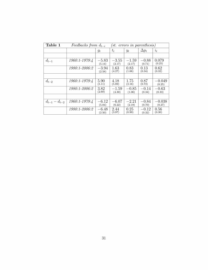
Table 1 Feedbacks from dt−i (st. errors in parenthesis)gt tt yt ∆pt it

dt−1 1960:1-1979:4 −5.83(5.14)

−3.55(2.17)

−1.59(2.17)

−0.88(0.71)

0.079(0.25)

1980:1-2006:2 −3.94(2.58)

1.63(4.27)

0.83(1.06)

0.13(0.34)

0.62(0.32)

dt−2 1960:1-1979:4 5.90(5.11)

4.18(5.89)

1.75(2.16)

0.87(0.72)

−0.049(0.25)

1980:1-2006:2 3.82(2.60)

−1.59(4.30)

−0.85(1.06)

−0.14(0.34)

−0.63(0.33)

dt−1 − dt−2 1960:1-1979:4 −6.12(5.04)

−6.07(6.22)

−2.21(2.19)

−0.84(0.70)

−0.038(0.27)

1980:1-2006:2 −6.48(2.50)

2.44(3.97)

0.25(0.99)

−0.12(0.32)

0.56(0.30)

31

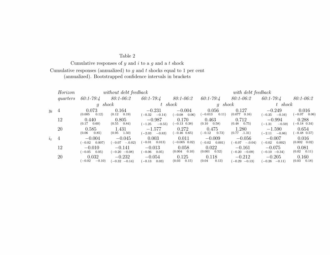
Table 2

Cumulative responses of y and i to a g and a t shock

Cumulative responses (annualized) to g and t shocks equal to 1 per cent(annualized). Bootstrapped confidence intervals in brackets

Horizon without debt feedback with debt feedbackquarters 60:1-79:4 80:1-06:2 60:1-79:4 80:1-06:2 60:1-79:4 80:1-06:2 60:1-79:4 80:1-06:2

g shock t shock g shock t shockyt 4 0.073

(0.005 0.12)0.164

(0.12 0.19)−0.231

(−0.32 −0.14)−0.004

(−0.08 0.06)0.056

(−0.013 0.11)0.127

(0.077 0.16)−0.249

(−0.35 −0.16)0.016

(−0.07 0.06)

12 0.440(0.17 0.60)

0.805(0.55 0.84)

−0.987(−1.25 −0.55)

0.170(−0.13 0.38)

0.463(0.10 0.58)

0.712(0.48 0.75)

−0.994(−1.31 −0.59)

0.288(−0.18 0.34)

20 0.585(0.06 0.85)

1.431(0.95 1.50)

−1.577(−2.03 −0.83)

0.272(−0.46 0.65)

0.475(−0.12 0.73)

1.280(0.77 .1.31)

−1.590(−2.11 −0.86)

0.654(−0.48 0.57)

it 4 −0.004(−0.02 0.007)

−0.045(−0.07 −.0.02)

0.003(−0.01 0.013)

0.011(−0.005 0.02)

−0.009(−0.02 0.001)

−0.056(−0.07 −.0.04)

−0.007(−0.02 0.002)

0.016(0.002 0.02)

12 −0.010(−0.05 0.05)

−0.141(−0.20 −0.08)

−0.013(−0.06 0.05)

0.058(0.004 0.10)

0.022(0.001 0.52)

−0.161(−0.20 −0.09)

−0.075(−0.10 −0.34)

0.081(0.02 0.11)

20 0.032(−0.02 −0.10)

−0.232(−0.32 −0.14)

−0.054(−0.13 0.03)

0.125(0.03 0.15)

0.118(0.04 0.13)

−0.212(−0.29 −0.13)

−0.205(−0.26 −0.11)

0.160(0.03 0.18)