NBER WORKING PAPER SERIES

CONSUMER DURABLES AND THE OPTIMALITY OF USUALLY DOING NOTHING

Avner Bar-lien

Alan S. Blinder

Working Paper No. 2488

NATIONAL BUREAU OF ECONOMIC RESEARCH 1050 Massachusetts Avenue

Cambridge, MA 02138 January 1988

We thank Andrew Abel, Ben Bernanke, and Sanford Grossman for useful comments, John Amer for research assistance, and the NSF for financial support. The research reported here is part of the NBER's research program in Economic Fluctuations.

Any opinions expressed are those of the authors and not those of the National Bureau of Economic Research. Support from The Lynde and Harry Bradley Foundation is gratefully acknowledged.

NBER Working Paper #2488 January 1988

Consumer Durables and the Optimality of Usually Doing Nothing

ABSTRACT

This paper develops a simple but important point which is often

overlooked: It is quite possible that the best policy for a rational,

optimizing agent is to do nothing for long periods of time—-even if new,

relevant information becomes available. We illustrate this point using the

market for durable goods. Lumpy costs in durables transactions lead

consumers to choose a finite range, not just a single level, for their

durables consumption. The boundaries of this range change with new

information and, in general, obey the permanent income hypothesis. However,

as long as the durable stock is within the chosen region, the consumer will

not change her stock. Hence individuals will make durable transactions

infrequently and their consumption can differ substantially from the

prediction of the strict PIH.

Such microeconomic behavior means that aggregate data cannot be generated

by a representative agent; explicit aggregation is required. By doing that,

we showed that time series of durable expenditures should be divided to two

separate series: One on the average expenditure per purchase and the other

on the number of transactions. The predictions of the PIH hold for the

former, but not for the latter. For example, the short-run elasticity of the

number of purchases with respect to permanent income is much larger than one

for plausible parameter values. We put our theory to a battery of empirical

tests. Although the tests are by no means always consistent with the theory,

most empirical results are in line with our predictions.

Avner Bar-Ilan Alan S. Blinder

Department of Economics Department of Economics

Tel-Aviv University Princeton University

Ramat-Aviv, ISRAEL Princeton, NJ 08544

The assumption of optimizing behavior Is the bedrock on which most of

economic theory stands. It is also the characteristic that, for better or for

worse, distinguishes economics from the other social sciences. Economists

are probably the only people on earth who believe -- or act as if they

believe -— that homo sapj behaves like homo economicus.

This paper does not question the hypothesis that people optimize.

(Probably, some other paper should.) Instead, it tries to square the

assumption of optimizing behavior with the coninon observation that human

behavior seems highly inertial. Like Newton's bodies at rest or in motion,

people often seem to cling to their past behavior despite clear evidence

calling for change. We will argue that the existence of lumpy costs of

changing a decision variable makes inertial behavior optimal under quite

general conditions. And we will illustrate this general idea with a detailed

analysis of a formal model of the purchase of consumer durables. one which

differs in some significant respects from the standard permanent income

hypothesis (PIH).

1. RATIONAL INERTIA: BASIC IDEAS

The standard type of optimizing behavior posited in economic models is

continuous reoptimizatlon. According to this view of behavior, the Individual

or firm controlling a decision variable, xt, Is given new constraints and/or

information each period (call that the vector zt), computes the value of the

decision variable that maximizes his objective function (call it 4), and

then sets xt=4 in every period. This optimum Is normally defined by some

kind of tangency condition. Examples abound. In consumption theory, x' is

consumption, zt Includes interest rates, current income and wealth, and

expectations about the future; the "Euler equation" Is based on the notion

1

that the consumer optimizes intertemporally in both period t and period t÷1.

In portfolio theory, xt is a vector of portfolio shares and zt includes

current wealth and the presumed varlance—covariance matrix; wealthhoiders

are supposed to adjust their portfolios every time their perceived

variance—covariance matrix changes.

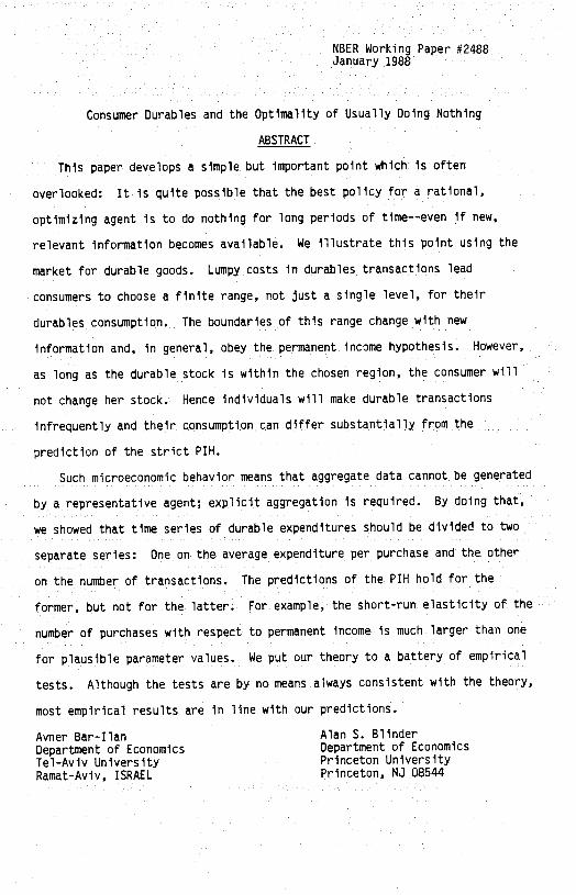
Figure 1 is a trivially simple graph displaying this general idea. Here

V(x;z) is the objective function, which moves any time z changes. The

decision maker Is assumed always to select x = argmax V(x;z) (point E), which induces a behavioral relation of the form xt = F(zt), Changes in z induce prompt responses In xt.

It seems doubtful, however, that many people behave this way ——

especially If the period is relatively short. (The authors of this paper

certainly don't.) Instead, people are alleged to be 'creatures of habit."

Econometric evidence certainly supports the general idea that behavior is

inertial. For example, empirically estimated decision rules of the form x = F(Zt) are almost always Improved by the addition of xt_1 to the righthand

side. Pervasive inertia seems to be a stylized fact of economic life.

Inertia may be irrational, as other social scientists will argue.

Laziness, procrastination, and other human frailties —— in general, a failure

to pursue one's best interests —— can all lead to inertial behavior. About

this, economists have little to say. But it Is also possible —— and this Is

the central point of the paper —— that Inertia can be rational when there are

lumpy costs of changing one's decision variable. It is easy to see why.

Ignoring, for the moment, how such costs might arise, suppose that our

prototypical decisionmaker incurs a fixed cost, b, each time he changes his

control variable. Now look back at Figure 1 and suppose that, because zt has

changed since the last decision period, the decislonmaker finds himself at a

2

I I

II $

II 'I II I II I

E

P

I

I I I I I

I V ( x ; z)

I

I I 1 K

s x xS t_i t

Fiture 1

Oontinuos Reoptimizatlon versus the (3,s) Rule

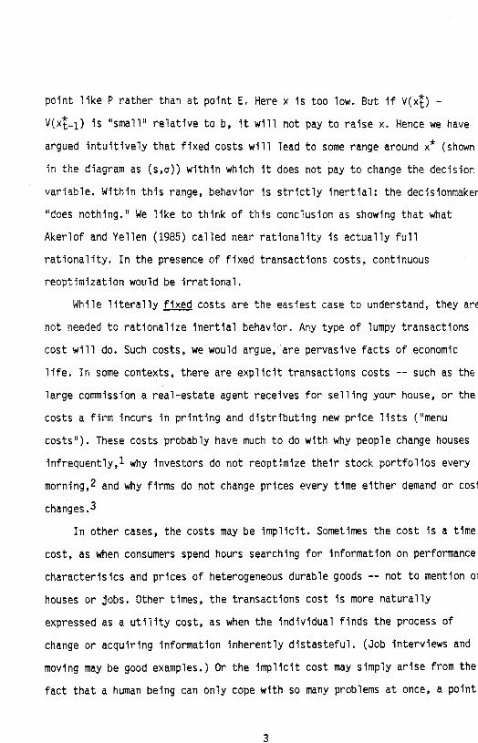
point like P rather than at point E. Here x is too low, But if V(x) —

V(x_1) Is 'small relative to b, It will not pay to raise x. Hence we have

argued intuitively that fixed costs will lead to some range around x (shown in the diagram as (s,a)) within which it does not pay to change the decision

variable, Within this range, behavior is strictly Inertial: the decisioninaker

"does nothing." We like to think of this conclusion as showing that what

Akerlof and Yellen (1985) called near rationality is actually full

rationality. In the presence of fixed transactions costs, continuous

reoptimization would be Irrational.

While literally fixed costs are the easiest case to understand, they ar€

not needed to rationalize inertial behavior. Any type of lumpy transactions

cost will do. Such costs, we would argue, are pervasive facts of economic

life. In some contexts, there are explicit transactions costs —— such as the

large commission a real-estate agent receives for selling your house, or the

costs a firm Incurs In printing and distributing new price lists ("menu

costs"). These costs probably have much to do with why people change houses

Infrequently,1 why Investors do not reoptimize their stock portfolios every

morning,2 and why firms do not change prices every time either demand or cost

changes .3

In other cases, the costs may be implicit. Sometimes the cost Is a time

cost, as when consumers spend hours searching for Information on performance

characterislcs and prices of heterogeneous durable goods —- not to mention ci

houses or jobs. Other times, the transactions cost Is more naturally

expressed as a utility cost, as when the individual finds the process of

change or acquiring Information inherently distasteful. (Job Interviews and

moving may be good examples.) Or the Implicit cost may simply arise from the

fact that a human being can only cope with so many problems at once, a point

3

often stressed by Herbert Simon. Hence there is a kind of "shadow cost" for

using the scarce resource of mental capacity. (Why else would CEOs delegate

decisions?>

Finally, some markets have large spreads between the prices at which you

can buy and sell, so that a buyer loses a lump of value the moment he takes

the good home. This type of lumpy cost is particularly prevalent in the

markets for consumer durables. One rationalization was provided by Akerlof

(1970), who argued that markets in which goods are heterogeneous and quality

is not readily observable are subject to the "lemons principle." (If this is

a good car, why are you selling It?) Whether or not caused by the lemons

principle, the gap between buying and selling prices may be a major reason

why any one consumer is active in the market for any particular durable only

sporadically. The rest of the time, he Is "doing nothing."

Of course, the econometric fact that xt_1 is almost always a significant

determinant of xt has been noti' 1 many times before. The usual "explanation"

is the partial-adjustment model, according to which convex costs of changing

x make it optimal to adjust xt to x gradually. Under the assumption that

adjustment costs are quadratic, a linear partial-adjustment rule like:

* xt - xt_1 = x(xt - xt_1)

can be derived from rigorous microfoundations. And so the assumption is

frequently made, usually without thinking twice about what it means.

There are two major problems with this common approach (and many others

in particular applications). The first is empirical: the estimated value of A

is almost always "implausibly slow" when interpreted as a speed of

adjustment. The second Is theoretical: while the existence of adjustment

costs is believable, the assumption that they are convex, much less

quadratic, is not in most applications. Think, for example, of money demand,

4

where the partial-adjustment model is almost universally employed. Can anyone

take seriously the hypothesis that the cost of changing your cash balance by

$100 rather than $99 greatly exceeds the cost of changing it by $1 rather

than zero? Or think about applying the quadratic assumption to adjustment

costs for installing fixed capital, where it has been used to rationalize the

Q-theory of investment,4 Does a firm really incur much higher adjustment

costs for the sixteenth drill press it installs than for the first? Other

examples could be listed. Frankly, we find it hard to think of many cases in

which the assumption of jaj marginal adjustment costs is more plausible than the assumption of riin, or even zero, marginal adjustment costs.

This is not just a minor theoretical quibble. While quadratic adjustment

costs make partial adjustment optimal, zero or decreasing marginal adjustment

costs make it optimal to adjust all at once or not at all. Look back at

Figure 1 once again. If the decisionmaker must pay a lumpy transactions cost

each time he changes x, he will not adjust x toward x* in small increments

period after period. Instead, he will either do nothing or jump all the way

to x* at once. Partial adjustment is simply too costly when transactions

costs are lumpy. (Think, for example, of the costs you would incur in selling

and buying a car every month,)

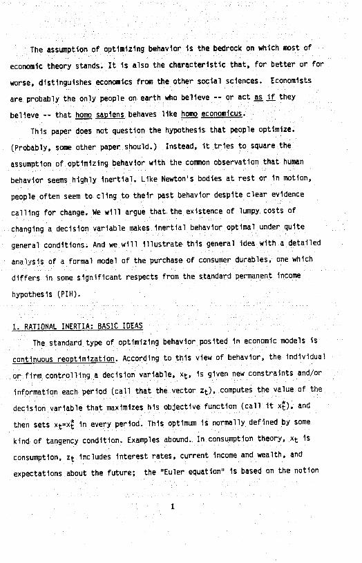
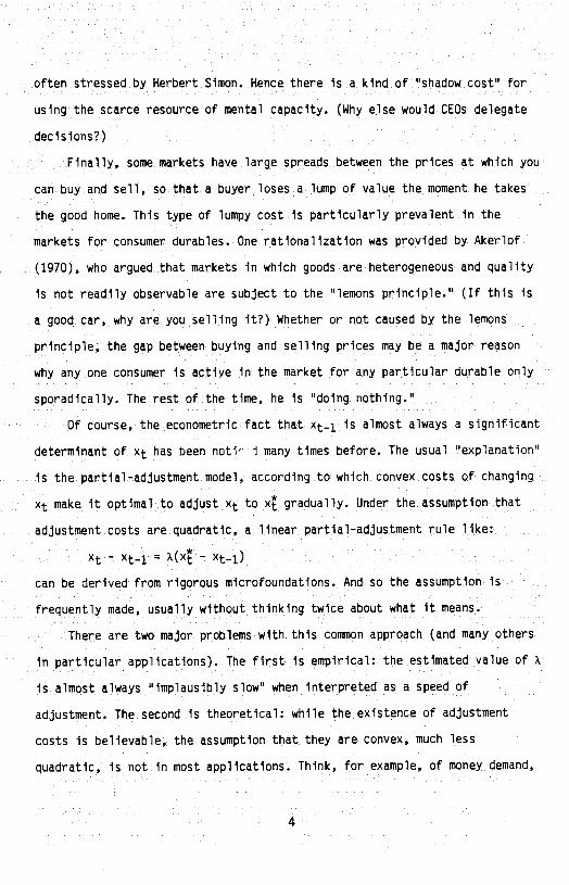
The case of fixed transactions costs has been extensively studied in the

inventory literature, where the so—called (S,s) or two—bin policy emerges as

the optimal strategy in awide range of circumstances. Specifically (see

Figure 2), firms facing i.i.d. demand shocks will find it optimal to set a

lower bound on inventory, s, and then tO restore inventories to S each time

that lower limit is reached. If demand is serially correlated, or if

something else is changing through time, the rule becomes an (St, t) policy.

5

Inventory Stock

Figure 2

The (S,s) :nventory Policy

time

We show below that the (St,st) rule is optimal for consumers buying

durables whose selling prices are lower than buying prices —— due, say, to

the lemons principle.5 But this is just one example of what we think is a

very general phenomenon. The same logic applies to business purchases of

capital goods, where adjustment cost functions are unlikely to resemble those

assumed by Q-theory, Instead, elements of fixed costs probably dictate that

an (S,s) rule be followed. Obviously, inventories are the application for

which (S,s) rules were invented; and (S,s) inventory management rules are

apparently in wide use. Switching to financial decisions, the Baumol-Tobin

model of transactions demand for money, when properly thought through

(remember the saw-tooth diagram?) is an (S,s) rule for money demand. And the

fixed cost of recalculating a variance-covarlance matrix to take account of

new information (and then of calling your broker with instructions) suggest

that optimal portfolios probably should follow a multi—dimensional (S,s) rule

rather than, say, the standard CAPH solution.6 As noted above, "sticky"

prices are probably more sensibly rationalized by fixed menu costs than by

quadratic adjustment costs. And the standard assumption in dynamic theories

of labor demand —— that a firm incurs rising marginal adjustment costs in

hiring new workers —— is difficult to believe. More likely, its marginal

adjustment costs are declining, in which case some kind of (S,s) rule will be

optimal rather than the partial—adjustment rule used, e.g., by Sargent

(1978).7

Finally, we offer an admittedly speculative application of (S,s)

reasoning to the debate over rational expectations. Suppose people really do

have rational (that is, model—consistent) expectations, but must pay a fixed

cost (in money, time, and/or disutility) each time they recalculate, say,

their expected rate of inflation by solving their multi-equation econometric

6

model. Then their actual expectations will exhibit inertial behavior: people

will stick to previous forecasts until they have good reason to believe that

recalculation will yield benefits large enough to repay the costs. At

the micro level, this sort of inertial behavior is quite different from

the gradual adjustment considered by Taylor (1975) and Friedman (1979).

Whether or not expectations appear close to adaptive at the macro level

depends on whether people change their forecasts asynchronously or all at

once.

In all these applications and more we believe that the particular

version of inertia embodied in (S,s) rules is a more plausible

characterization of optimal behavior than the partial-adjustment model. But

the discussion so far has been entirely intuitive. It Is now time to prove

that the (S,s) rule is optimal for purchases of consumer durables.

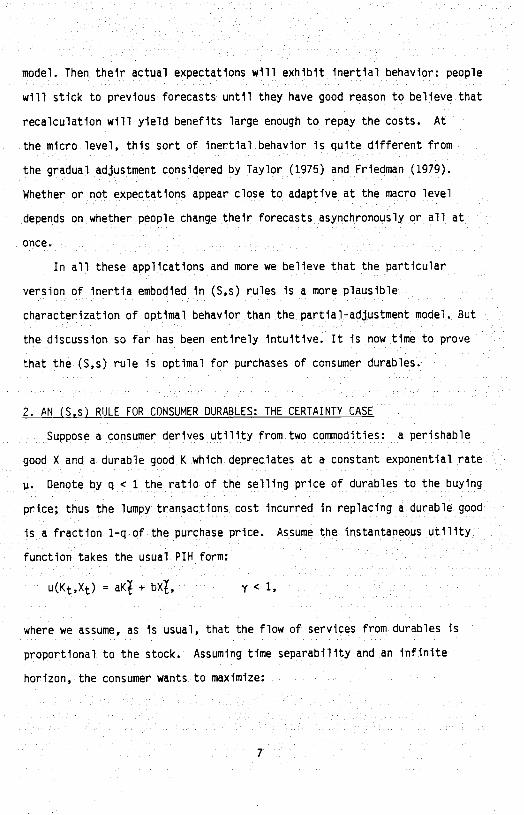
2. AN (S,s) RULE FOR CONSUMER DURABLES: THE CERTAINTY CASE

Suppose a consumer derives utility from two comodities: a perishable

good X and a durable good K which depreciates at a constant exponential rate

i. Denote by q < 1 the ratio of the selling price of durables to the buying

price; thus the lumpy transactions cost incurred in replacing a durable good

Is a fraction 1—q of the purchase price. Assume the instantaneous utility

function takes the usual PIH form:

u(Kt,Xt) = aK + bX, y < 1,

where we assume, as is usual, that the flow of services from durables is

proportional to the stock. Assuming time separability and an infinite

horizon, the consumer wants to maximize:

7

U = J u(Kt,Xt)etdt, 0

where p is the rate of subjective time discounting.

It is clear that, because of the lumpy transactions costs, durable

purchases will take place only occasionally, for continuous replacement would

imply infinite transactions costs. Let durables be purchased at dates t1,

t2,..., and let Sn denote the durable stock immediately after the nth durable

purchaseS (By notational convention, let denote the opening stock, that

is, S0 K0.) That good will be replaced at time t÷j, by which time it has

deteriorated to a value s given by:

(1) sn=Sne

Thus the discounted utility obtained while the nth "car1 is held will be:

tn+1 (ttn) - t J u{s e , x}e dt

tfl

Summing over all lifetime purchases of durables and using the specific

functional form yields the following expression for lifetime utility:

—(ty+p)t —(iiy+p)t+i (2) U = tal(uy+p)] E [e

— e j(Sn e11 fl)1] n=Q

+ b f e_Pt(Xt)1 dt ,

0

which is homogenous of degree In its arguments [S0, S1, S2,. .} and X.

To derive the budget constraint, let the nondurable good be the numeraire

and assume that the relative price of durables to nondurables is a constant,

p. Hence the resale price of "one unit" of the durable good is qp. At time

8

t, n > 1, net expenditure on durables is, therefore:

(3) En pS —

qps_1 =

PSn —

qpS_1 e

With this definition, the lifetime budget constraint is simply:

-rt

(4) W = f e't Xtdt + Z Ene

'

0 n=i

where W denotes total (human and nonhuman) lifetime wealth exclusive of

durables. Notice that the budget constraint is linearly homogenous in its

arguments X and S0. S1, S2

The intertemporal optimization problem of the consumer is to maximize (2)

subject to (4) and given K0. The solution consists of a plan for nondurable

consumption, Xt, and two infinite series of trigger points {S1, S2, . . .} and

(s0, Si *..) which denote the stocks immediately after the purchase and

just before resale, respectively. This is a complicated problem; but the

homogeneity of lifetime utility and the linearity of the budget constraint

simplify the solution significantly and reduce the Infinite number of

parameters in the s and S series to only three: s0 and fixed ratios,

S1-÷/S and Sn/Sn for n > 1. Similarly, as in the standard PIll, the

nondurable consumption plan, Xt, is characterized by only two parameters:

initial consumption and a constant exponential growth rate. Moreover, the

growth rates of the consumption plans of both goods are the same, which

reduces the total number of parameters to four. All this is summarized in

the following theorem:

Theorem 1:8 The optimal consumption plan (S, s, X) has the following

properties:

9

(i) X0, {S1,S2,,..) and {so,sl,s2,...) are all homogeneous of degree

one in the vector (W, K0).9

(ii) The ratio s,/S defined by (1) Is the same for all n > 0, meaning

that the interval between purchases, •r, Is constant.

(iii) The ratio S÷1/S, for n > 0 is constant and equal to e9 where

g

Proof:

It is easier to prove the theorem by defining the consumption plan by

(S,t,X), where t is the vector of purchase dates, than by (S,s,X). We want

to show that if (S*,t*,X) is the optimal consumption plan when wealth is (W,

K0) then (cS*,t*,cXt) is optimal when wealth is (cW cK0). Since the budget

constraint is linear, the feasibility of (S*,t*,X) with wealth (W, K0)

immediately implies that (cS*,t*,cX) Is feasible with wealth (cW, cK0). The

homogeneity of the utility function implies that If (S*,t*,X) is preferred

to (S',t,X), then (cS*,t*,c4) is preferred to (cS',t',cX) for every c >

0, Therefore (cS*,t*,cX) is optimal with wealth (cW, cK0) and part (1) of

the theorem is established.

The above applies to the optimal consumption plan starting at time 0.

But since the utility function is assumed to be stationary and the horizon is

infinite, the same comparisons can be made at other starting times.

Therefore, the optimal consumption plan beginning at time t1 will be

($S*,t*,14), if the new vector of wealth is ($W, AK) for some constant $.

As a result t2 - t1 = t1 — t0, and furthermore tn+1 — tn = t, the same

constant. Since equation (1) is s,/S = ett and t is a constant, part (ii) is proved.

10

The proportionality of both components of consumption to lifetime wealth

means that a constant fraction, h, of wealth is allocated to durable

consumption each time a new purchase is made. This constant is defined as:

(5) h pS/W.

At the moment just before the (n+1)—st purchase is made, the consumer (who

last bought a durable at time — r) holds

(W — pS)erT

in financial wealth and

qpSeIt

in durables. Hence:

(6) Wn+i = (Wn — pSn)&'t ÷ qpS e1T

Since Sn+i/Sn = Wn+1/Wn we can divide both sides of equation (6) by W to

get,

Sn+i/Sn Wn+i/Wn (1_pS/W)ert + (qpSnt4)et = (1_h)er + qhewr

which is a constant, as specified in part (iii) of the theorem.

The separability of both the utility function and the budget constraint

in durables and nondurables implies that what was proved for the former holds

for the latter as well. In particular part (iii) of Theorem 1 means that the

growth rate of nondurable consumption, denoted by g, is constant. Similarly

the ratio of consumption at time t, X(tn), to wealth at time t, W, is a

constant. Hence:

X(tn+i) — — S÷1 (7)

X(t) — —

which is a constant. Since Xt grows at an exponential rate g, (7) implies

that = e for n > 0, which establishes part (iii) and completes the

11

proof of Theorem 1. Q.E.O.

Where nondurables are concerned, Theorem I simply repeats the standard

implications of the PIH, omitting the obvious (but important) point that the

time pattern of income is irrelevant to the time pattern of consumption

('transitory income doesnt matter'). This, of course, is a direct product of

our assumption of separability in the utility function. For durables,

however, Theorem 1 modifies the PIH in several important respects.

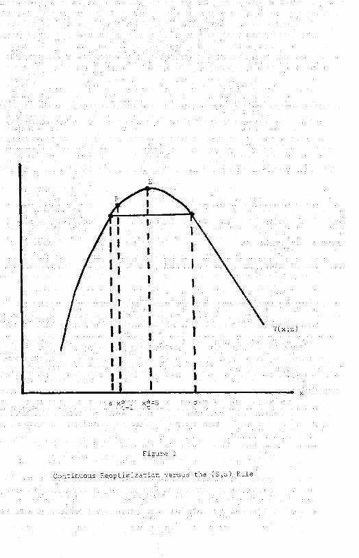
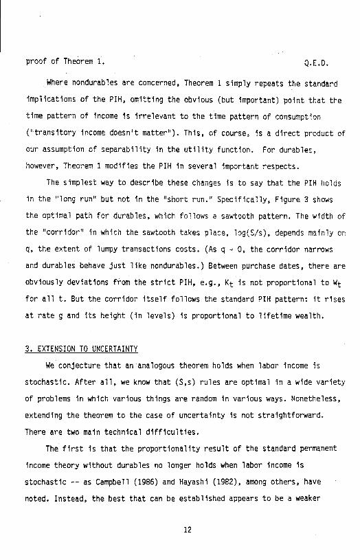
The simplest way to describe these changes is to say that the PIN holds

in the "long run' but not in the "short run.' Specifically, Figure 3 shows

the optimal path for durables, which follows a sawtooth pattern. The width of

the "corridor" in which the sawtooth takes place, log(S/s), depends mainly on

q, the extent of lumpy transactions costs. (As q -* 0, the corridor narrows

and durables behave just like nondurables.) Between purchase dates, there are

obviously deviations from the strict PIN, e.g., Kt is not proportional to Wt

for all t. But the corridor itself follows the standard PIN pattern: It rises

at rate g and its height (In levels) is proportional to lifetime wealth.

3. EXTENSION TO UNCERTAINTY

We conjecture that an analogous theorem holds when labor income is

stochastic. After all, we know that (S,s) rules are optimal in a wide variety

of problems in which various things are random in various ways. Nonetheless,

extending the theorem to the case of uncertainty is not straightforward.

There are two main technical difficulties.

The first is that the proportionality result of the standard permanent

income theory without durables no longer holds when labor income Is

stochastic —— as Campbell (1986) and Hayashi (1982), among others, have

noted. Instead, the best that can be established appears to be a weaker

12

0be

÷HHHHH÷HHII4-,

H÷HHIIHp+Hc-I4-,H4-,0p

4-'4-'

PP

Hbe00

homogeneity result. For example, Hayashi (1982) assumes constant relative

risk aversion utility and that labor income is given by:

Yt = (1 + et),

where is constant and et is a white noise disturbance, The latter is a very

restrictive and empirically unattractive specification. However, It enables

him to prove that optimal consumption is homogeneous of degree one In the

vector (,A), where A Is nonhuman wealth. Notice that consumption Is not

proportional to A + H, where H is "human wealth,' i.e., the expected

discounted present value of earnings. Instead, the ratio A/H affects

consumption. Since our Theorem 1 essentially grafts an (S,s) approach to

durabies onto the standard PIH, we cannot expect the proportionality result

to hold under uncertainty,

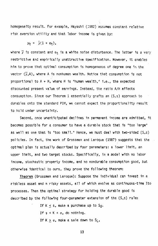
Second, once unanticipated declines in permanent income are admitted, it

becomes possible for a consumer to have a durable stock that is "too large

as well as one that is "too small." Hence, we must deal with two-sided (S,s)

policies. In fact, the work of Grossman and Laroque (1987) suggests that the

optimal plan is actually described by four parameters: a lower limit, an

upper limit, and two target stocks. Specifically, in a model with no labor

Income, stochastic property income, and no nondurable consumption good, but

otherwise identical to ours, they prove the following theorem:

Theorem (Grossman and Laroque): Suppose the individual can Invest in a

riskless asset and n risky assets, all of which evolve as continuous—time Ito

processes. Then the optimal strategy for holding the durable good is

described by the following four—parameter extension of the (S,s) rule:

If K < s, make a purchase up to Sj. If s K< a, do nothing.

If K > a, make a sale down to SL,

13

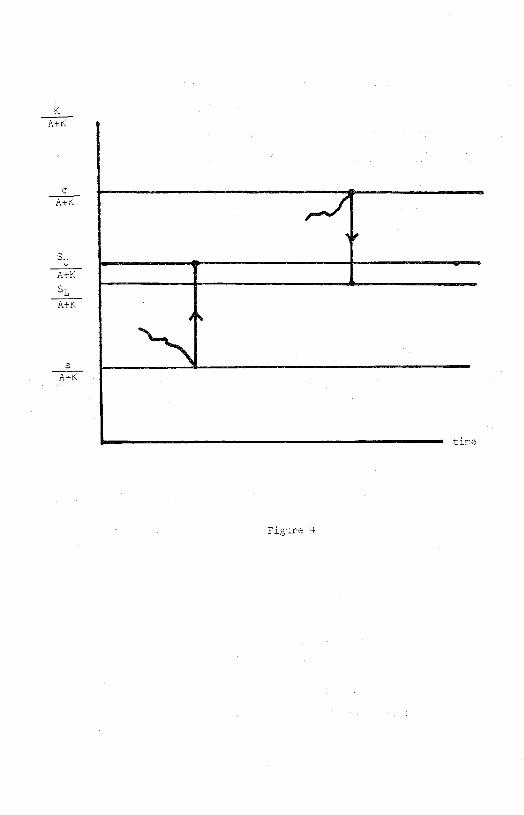
where (S,SL, SU, a) are all proportional to total wealth, A + K.

Figure 4 depicts this rule. As the graph shows, SL is smaller than S,

which seems odd at first. The reason Is that transactions costs lost in

selling a large durable good of size a exceed those lost In selling a small

durable of size .10

HayashUs result and Grossman and Laroque's theorem lead us to the

following conjecture for our model with durables:

Conjecture: Suppose the interest rate and the depreciation rate are

nonstochastic, the utility function is as assumed before, and human wealth

evolves according the Ito process:

dH/H = gdt + wdz,

where dz is a standard Weiner process. Then the (s ,SL, S, a) rule described

above is optimal and all four parameters are homogeneous of degree one in the

vector (A, H, K).

Notice that we do not claim that s, SL, Su and a are proportional to

total wealth. That is probably untrue. Under uncertainty, ratios like s/(A+H)

and a/(A-FH) presumably depend on the composition of wealth, just as in

Hayashi's case. For example, since s is a linearly homogeneous function of

(K,A,H):

s = f(K,A,H),

we know that:

s/H = f(K/H,A/H,1).

At any moment at which the lower barrier is hit, K = 5, so:

s/H = f(s/H, A/H, 1),

which defines s/H as a function of A/H. Grossman and Laroque's theorem

14

U :L

proves, for their case, that this function has only one root.

We cannot simply adapt their proof because human capital is a nontraded

asset, whereas all of their assets are freely tradable. The technical problem

is that, while Grossman and Laroque can reduce their two state variables (K

and A) to one, the best we can do is to reduce our three state variables (K,

A, and H) to two. That makes the problem enormously more difficult and their

proof inapplicable to our case. We can, however, establish the homogeneity

result conditional on the (s, SL, S, a) rule being optimal. Specifically, we

can prove:

Theorem 2: If the (s, SL, Su a) strategy is optimal, then s, SL, S,

and a are all homogeneous of degree one in the vector (A, H, K).

Proof: The proof simply follows the logic of the first part of the proof

of Theorem 1. FIrst we show that if a strategy (s, SL, S, a) is feasible

when the wealth vector is (A, H, K), then a strategy (bs, bSL, bS1j, ba) is

feasible when the wealth vector Is (bA, bH, bK). To see this, start by

writing the laws of motion that hold whenever a durable purchase is not made:

dH/H = gdt + wdz

dK/dt = - pIK

dA/dt = rA + y -

where y Is labor Income, defined by:

y = rH — dH/dt.

Clearly, these are all linear homogeneous. Furthermore, at instants at which

a durable purchase is made, we have:

15

A+-A=_Et =-[pS -p j tn tn fl n n-I

K+-K=St - tn tn fl t

which are also linear homogenous. Thus, if A, H, y and K are all multiplied

by any constant b, we get a feasible solution by multiplying X, s, SL, S,

and o by the same constant b. Given feasibility, optimality follows directly

from the homogeneity of the utility function, just as before.

4, AGGREGATE IMPLICATIONS

Though the (S,s) rule rests on solid microfoundations and is probably

optimal in a wide variety of problems, it has not been used much in economics

because of the difficulties It poses for aggregation. Clearly, the fiction of

a representative agent will no longer do because decislonmakers hit their

trigger points at different times. In the context of consumer durables, the

whole economy at any one time consists of a small number of people who spend

a lot and a large number of people who spend zero. Critics of the (S,s)

approach argue either that It cannot be aggregated or that, once aggregated,

it just leads back to the partial—adjustment model. But, as one of us showed

several years ago (Blinder, 1981a), neither is quite true. This section is

devoted to drawing out the aggregate implications of the (S,s) model of

individual purchases of consumer durables.

As usual, exact aggregation Is not possible In full generality; special

assumptions must be invoked. We allow Individual consUmers to differ In two

respects. First, people with the same (permanent) Incomes will not hold the

same stocks of durables because of different past histories. Rather, they

will be at different points within the relevant (S,s) range. Second, people

16

have different permanent incomes, and hence different optimal (S,s) ranges.

For concreteness, we assume that there are n income groups with permanent

incomes (ordered from highest to lowest) y, Y2, •, Y and, correspondingly, n monitoring ranges, (S1,s1), ...,

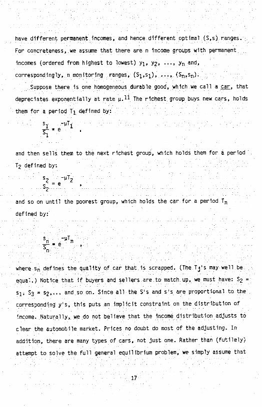
Suppose there is one homogeneous durable good, which we call a car, that

depreciates exponentially at rate i.11 The richest group buys new cars, holds

them for a period T1 defined by:

s1

1

and then sells them to the next richest group, which holds them for a period

12 defined by:

-p12

2

and so on until the poorest group, which holds the car for a period Tn

defined by:

s -

where 5n defines the quality of car that is scrapped. (The Tj's may well be

equal.) Notice that if buyers and sellers are to match up, we must have: S2 =

s1, S3 = 2'•• and so on. Since all the S's and S'S are proportional to the corresponding y's, this puts an implicit constraint on the distribution of

income. Naturally, we do not believe that the income distribution adjusts to

clear the automobile market. Prices no doubt do most of the adjusting. In

addition, there are many types of cars, not just one. Rather than (futilely)

attempt to solve the full general equilibrium problem, we simply assume that

17

the income distribution is 1right. This is, of course, "one of those

aggregation assumptions.1' But it seems a big improvement over assuming that

everyone is alike.

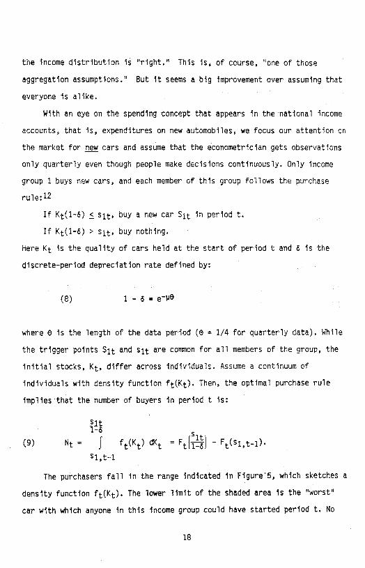
With an eye on the spending concept that appears in the national income

accounts, that is, expenditures on new automobiles, we focus our attention on

the market for new cars and assume that the econometriclan gets observations

only quarterly even though people make decisions continuously. Only income

group 1 buys new cars, and each member of this group follows the purchase

rule:12

If Kt(1-6) < s, buy a new car Sit in period t. If Kt(1—) > s, buy nothing.

Here Kt is the quality of cars held at the start of period t and is the

discrete—period depreciation rate defined by:

(8) 1-=e0

where 8 is the length of the data period (9 = 1/4 for quarterly data). While

the trigger points and sit are common for all members of the group, the

Initial stocks, Kt, differ across individuals. Assume a continuum of

individuals with density function ft(Kt). Then, the optimal purchase rule

implies that the number of buyers in period t is:

1-6

Nt = I dKt

— Ft(sj,t...1).

51,t—1

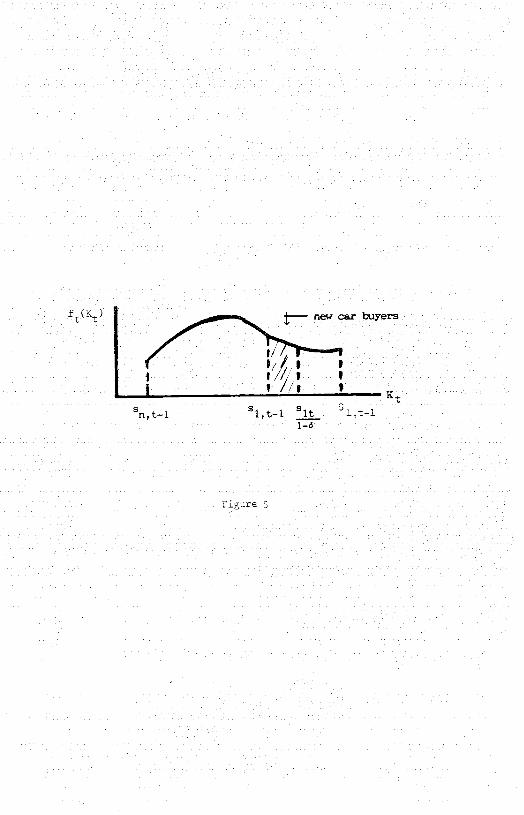
The purchasers fall in the range indicated in Figure5, which sketches a

density function ft(Kt). The lower limit of the shaded area is the "worst"

car with which anyone in this income group could have started period t. No

18

a)

p

pCr)

U)

'-4

U)

pp

one in the top income group is to the left of sl,t_1. The upper limit of the

shaded area is the lowest quality car that will be kept. Anyone to the right

Sit of will keep his car (at least until next period). Everyone who buys

spends the same amount, Ct = Sit, so total expenditures on new cars in

period t are:

(10) Et CtNt = Sit[ Ff} -

Equation (10) is the market demand function for durables implied by the

(S,s) theory; so the aggregation problem has now been solved. However, the

Implications of (10) are far from transparent. To begin with, it may help to

work out a concrete example. The most obvious benchmark is the steady state

distribution of f(K). In a steady state, the age distribution of cars is

n

uniform between 0 and T E Ij;

that is, if h denotes age, the density j=i

function of age is:

f(h)=i/T 0<h<T = 0 otherwise

Age and automobile quality are related by:

K = S1 eh

So, by the usual formula for change-of-variables:

f(K) = ]f(h) = 5 < K < S1

Thus the cumulative distribution function needed for (9) is:

logK-logs

(ii) F(K) = s < K S1

19

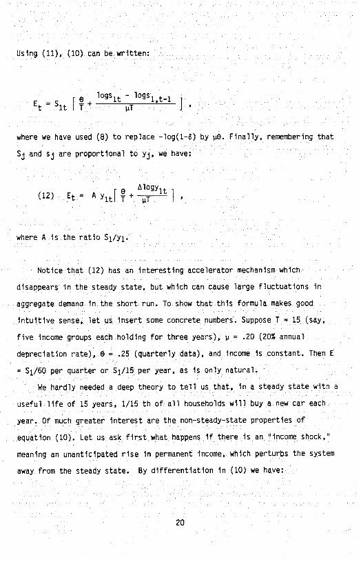
Using (11), (10) can be written:

e logs1 —

logs1 — E—S —+ ' 1

t 1tLT I'

where we have used (8) to replace —log(1-6) by iiO. Finally, remembering that

Sj and sj are proportional to yj, we have:

Alogy (12) Et = A Yit[ T +

.iT I

where A is the ratio S1/y1.

Notice that (12) has an interesting accelerator mechanism which

disappears in the steady state, but which can cause large fluctuations in

aggregate demand in the short run. To show that this formula makes good

intuitive sense, let us insert some concrete numbers. Suppose I = 15 (say,

five income groups each holding for three years), j = .20 (20% annual

depreciation rate), e = .25 (quarterly data), and income is constant. Then E

= S1/60 per quarter or S1/15 per year, as is only natural.

We hardly needed a deep theory to tell us that, in a steady state with a

useful life of 15 years, 1/15 th of all households will buy a new car each

year. Of much greater interest are the non-steady-state properties of

equation (10). Let us ask first what happens if there is an 'income shock,"

meaning an unanticipated rise in permanent income, which perturbs the system

away from the steady state. By differentiation in (10) we have:

20

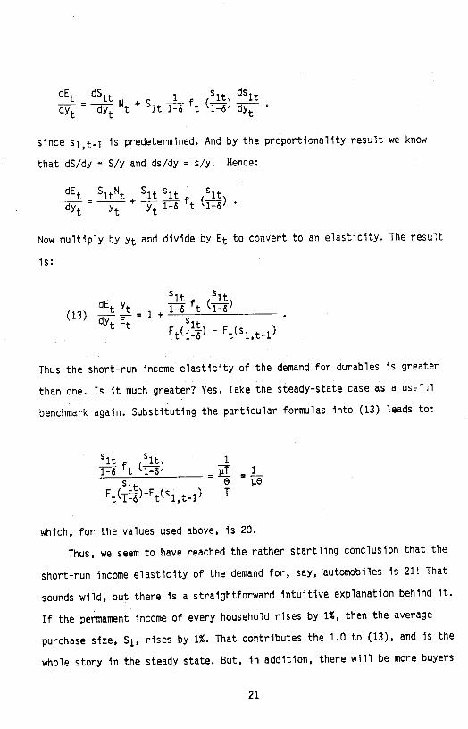
dE dS s ds

dYt

— t t It 1- t i—s

since sl,t_1 is predetermined. And by the proportionality result we know

that dS/dy = Sly and ds/dy = s/y. Hence:

dE SN S s s

t t

Now multiply by Yt and divide by Et to convert to an elasticity. The result

is:

S1 Sit dtY —f (—) (13) —-=1+

-

t t F'1' F' —

Thus the short—run income elasticity of the demand for durables is greater

than one. Is it much greater? Yes. Take the steady—state case as a used' 1

benchmark again. Substituting the particular formulas into (13) leads to:

sit sit 1

s1 -

e The Ft(---)-Ft(siti)

which, for the values used above, is 20.

Thus, we seem to have reached the rather startling conclusion that the

short—run income elasticity of the demand for, say, automobiles is 21! That

sounds wilds but there is a straightforward intuitive explanation behind it.

If the permament income of every household rises by 1%, then the average

purchase size, S1. rises by 1%. That contributes the 1.0 to (13), and is the

whole story in the steady state. But, in addition, there will be more buyers

21

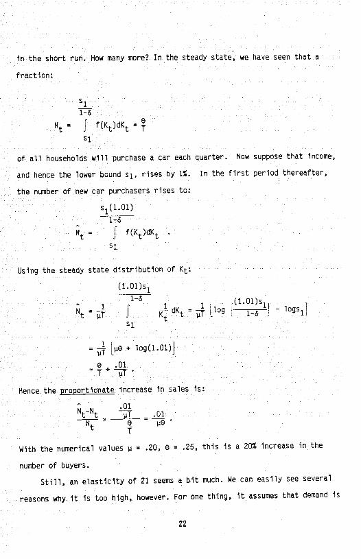
In the short run. How many more? In the steady state, we have seen that a

fraction:

Si

Nt I f(Kt)dKt =

Si

of all households will purchase a car each quarter. Now suppose that income,

and hence the lower bound s1, rises by 1%. In the first period thereafter,

the number of new car purchasers rises to:

s1(1.01) 1—&

Nt I f(Kt)dKt

Using the steady state distribution of Kt:

(1.01)s1

101 =

dKt = [log [ •Sij - logs1l

= — [.te + log(1.O1)

+ I iT

Hence the proportionate increase in sales is:

01 Nt_Nt — .01

e T

With the numerical values = .20, 0 = .25, this is a 20 increase in the

number of buyers.

Still, an elasticity of 21 seems a bit much. We can easily see several

reasons why it is too high, however. For one thing, it assumes that demand is

22

always met at unchanged prices. In reality, a sudden 20% increase in demand

might encounter rising supply price. For another, a 1% rise in GNP does not

raise everyone's (permanent) income by 1%, even if we ignore the distinction

between permanent and current income. Some people in the relevant range will

experience income increases much greater than 1%; but they will still raise

their car purchases from zero to one, not to two or three. Others will

experience no increase at all, and hence will not demand more cars. So, as Is

usual, heterogeneity tends to smooth things out. Finally, it is worth

pointing out that quarter-to-quarter changes in purchases of durable goods

are quite variable; 20% increases or decreases are not unheard of, especially

for automobiles.

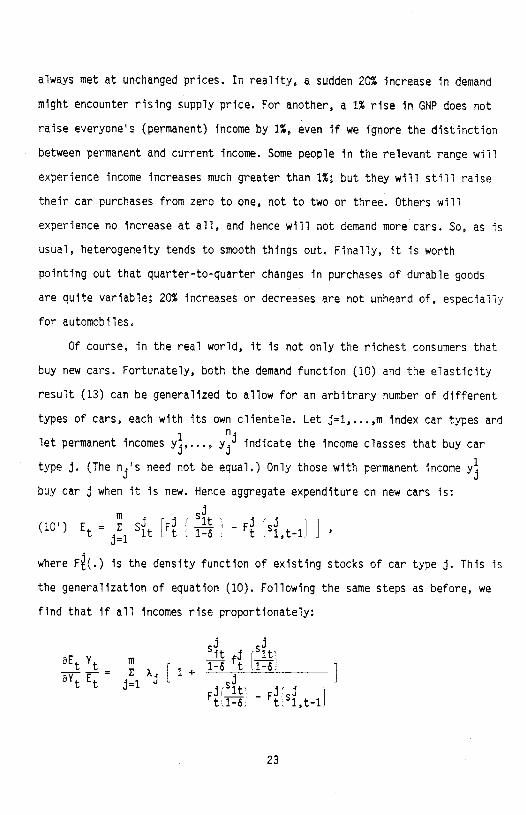
Of course, in the real world, It Is not only the richest consumers that

buy new cars. Fortunately, both the demand function (10) and the elasticity

result (13) can be generalized to allow for an arbitrary number of different

types of cars, each with its own clientele. Let j=1,. . . ,in index car types and

let permanent incomes y,..., yj1 indicate the income classes that buy car

type j. (The nfs need not be equal,) Only those with permanent income y buy car j when It is new, Hence aggregate expenditure on new cars Is:

(10') Et = s [F [5] - F [S1] 1

where F(.) is the density function of existing stocks of car type I. This is

the generalization of equation (10). Following the same steps as before, we

find that if all incomes rise proportionately:

S1 S —f —f = 1 1 + aYE ii I

Filt F1 .1 — tsl,t-1

23

where Aj is the weight of car type j. Around the steady state, with .t, T and

0 common to all cars, we get:

aEY 1

the same result as before.

It is interesting to compare the predicted short-run income elasticity

(say. 21) to the corresponding elasticity in the stock—adjustment model:

(14) Et = A(yt - Kt) +

Taking the derivative and converting to an elasticity around the steady state

(where E = K and K = y), gives:

dyE &'

which can certainly exceed unity. However, for this elasticity to be far

above unity, the speed of adjustment must be a large multiple of the

depreciation rate, which Is not only unlikely but runs counter to empirical

estimates.

In fact, a well-known problem with stock-adjustment models is that they

tend to produce implausibly small estimated "speeds of adjustment" —- the

coefficient A. The (S,s) model gives this econometric parameter an entirely

different interpretation, however. It follows from (10) that:

S eK lttl—6

where denotes the effect of a uniform rightward shift of the density

function of Initial stocks. Using the steady—state density function

and the fact that:

24

e1

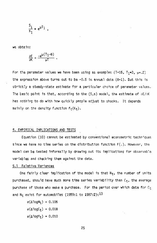
we obtain:

oE — _eT10) - i.iT

For the parameter values we have been using as examples (T=15, T1=3, ii=.2)

the expression above turns out to be —0.5 in annual data (0=1). But this is

strictly a steady—state estimate for a particular choice of parameter values.

The basic point is that, according to the (S,s) model, the estimate of 8E/8K

has nothing to do with how quickly people adjust to shocks. It depends

mainly on the density function ft(Kt),

5. EMPIRICAL IMPLICATIONS AND TESTS

Equation (10) cannot be estimated by conventional econometric techniques

since we have no time series on the distribution function F(,). However, the

model can be tested informally by drawing out its implications for observable

variables and checking them against the data.

5.1 Relative Variances

One fairly clear implication of the model is that Nt, the number of units

purchased, should have much more time series variability than Ct, the average

purchase of those who make a purchase. For the period over which data for Ct

and Nt exist for automobiles (1959:1 to 1987:2):13

(AlogN) = 0.106

a(logC) = 0.018

a(AlogY) = 0.010

25

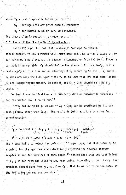
where t = real disposable income per capita

Ct = average real car price paid by consumers

Nt = per capita sales of cars to consumers.

The theory clearly passes this crude test.

5.2 Tests of the "Random Walk" Hypothesis

Hall (1978) pointed out that nondurable consumption should,

approximately, follow a random walk. More precisely, no variable dated t-1 or

earlier should help predict the change in consumption from t-1 to t. Since in

our model the variable Ct should follow the standard PIH precisely, Hall's

tests apply to this time series directly. But, according to the (S,s) model,

Mt does not obey the PIH. Specifically, it follows from (9) that both lagged

Nt and lagged income matter. So both Mt and Et = CtNt should fall Hall's

tests.

We test these implications with quarterly data on automobile purchases

for the period 1960:1 to 1987:2.14

First, following Hall, we ask if Et = CtNt can be predicted by Its own

past values, other than Et_i. The result is (with absolute t—ratios in

parentheses):

Et = constant + 0.66Et_1 + 0.23Et_2 — 0.O8Et_3 - 0,O2Et4 (7.0) (2.3) (0.9) (0.2)

= .77; OW = 1.99; F(392) = 1.89 (p = .14).

The F test fails to reject the omission of longer lags; but that seems to be

a quirk, for the hypothesis was decisively rejected for several shorter

samples in earlier versions of this paper.15 Notice also that the coefficient

of Et_1 is far from the usual value, near unity. According to our theory, the

problems should come from Nt, not from Ct. That turns out to be the case, as

the following two regressions show.

26

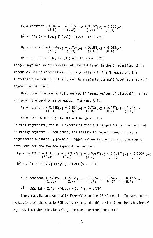
Ct = constant + 0.87Ct_i + 0.l6Ct_2 + 0.19Ct.3 — 0.2OCt_4 (8.8) (1.2) (1.4) (1.9)

R2 = .98; OW = 1.93; F(3,92) = 1.99 (p .12)

Nt = constant + 0.73Nt.i + 0.29Nt2 - 0.15Nt3 + 0.03Nt4 (7,9) (2,8) (1.5) (0.4)

= .85; OW 2.02, F(3,92) = 3.33 (p = .023)

Longer lags are inconsequential at the 10% level in the Ct equation, which

resembles Halls regressions. But Nt_2 matters In the Nt equation; the

F-statistic for omitting the longer lags rejects the null hypothesis at well

beyond the 5% level.

Next, again following Hall, we ask if lagged values of disposable income

can predict expenditures on autos. The result is:

Et = constant + 0.7lEt_i + 0.88Vt_i — 0.7OVt_2 + 0.O6Yt_3 — 0.26Vt_4 (11.4) (3.4) (2.0) (0.2) (1.0)

R2 = .79; OW = 2.30; F(4,91) = 3.47 (p = .011)

In this regression, the null hypothesis that all lagged V's can be excluded

Is easily rejected. Once again, the failure to reject comes from some

significant explanatory power of lagged income in predicting the number of

cars, but not the averaqe expenditure per car:

Ct = constant + 1.OOCt1 — 0.0003Yt_i — O.0023Yt_2 + O.0O37Yt_3 — 0.0009Yt_4 (50.0) (0.2) (1.3) (2.1) (0.7)

R2 = .98; OW = 2,17; F(4,91) = 1.90 (p = .12)

Nt = constant + 0.S3Nt_i + — 6.90Vt2 — 0.74Yt_3 — (17.5) (2.7) (1.7) (0.2) (0.2)

R2 = .86; OW = 2.49; F(4,91) = 3,07 (p = .020)

These results are generally favorable to the (S,s) model. In particular,

rejections of the simple PIH using data on durables stem from the behavior of

Nt, not from the behavior of Ct, just as our model predicts.

27

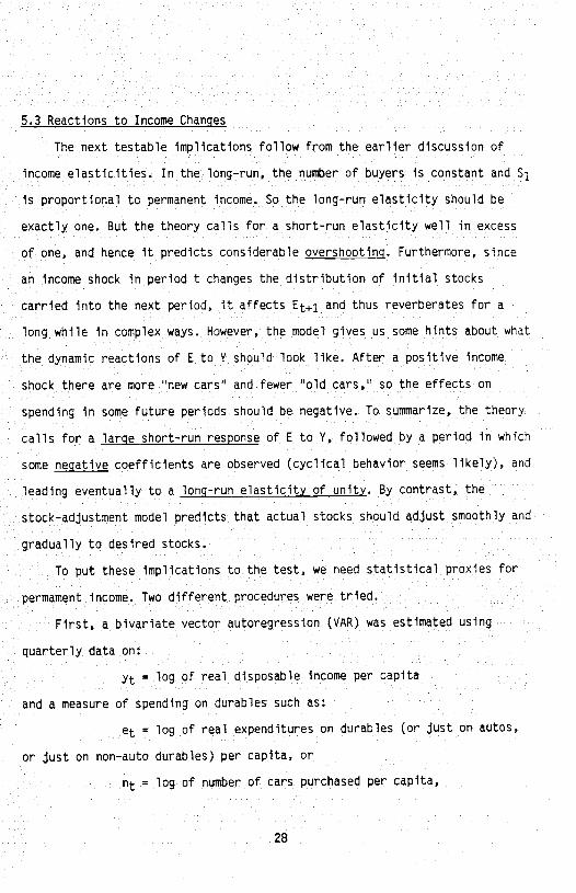
5.3 Reactions to Income Changes

The next testable implications follow from the earlier discussion of

income elasticities. In the long—run, the number of buyers is constant and S1

is proportional to permanent income. So the long—run elasticity should be

exactly one. But the theory calls for a short—run elasticity well in excess

of one, and hence it predicts considerable overshooting. Furthermore, since

an income shock in period t changes the distribution of initial stocks

carried into the next period, it affects Et+i and thus reverberates for a

long while in complex ways. However, the model gives us some hints about what

the dynamic reactions of E to V should look like. After a positive income

shock there are more "new cars" and fewer 'old cars,' so the effects on

spending in some future periods should be negative. To summarize, the theory

calls for a large short—run response of E to Y, followed by a period in which

some negative coefficients are observed (cyclical behavior seems likely), and

leading eventually to a long-run elasticity of unity. By contrast, the

stock-adjustment model predicts that actual stocks should adjust smoothly and

gradually to desired stocks.

To put these implications to the test, we need statistical proxies for

perniament income. Two different procedures were tried.

First, a bivariate vector autoregression (VAR) was estimated using

quarterly data on:

Yt = log of real disposable income per capita

and a measure of spending on durables such as:

et = log of real expenditures on durables (or just on autos,

or just on non-auto durables) per capita, or

= log of number of cars purchased per capita,

28

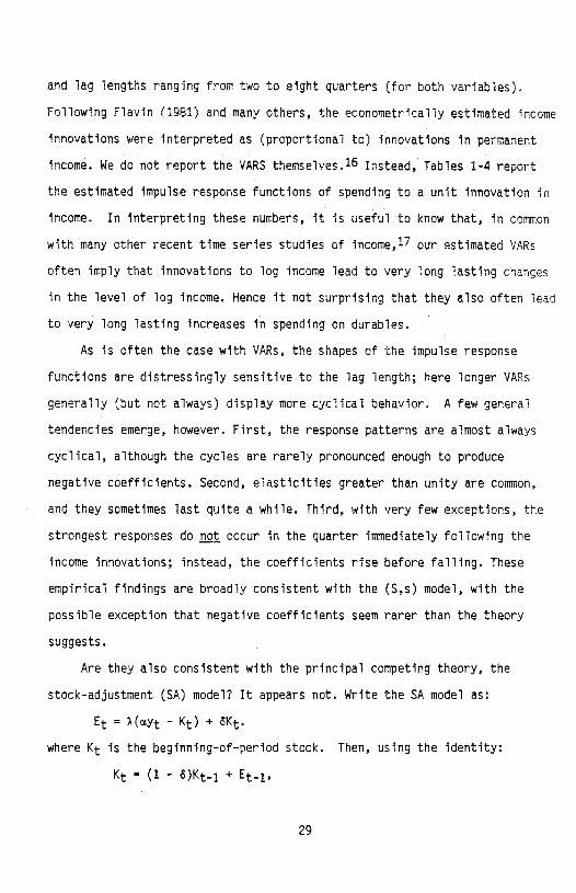
and lag lengths ranging from two to eight quarters (for both variables).

Following Flavin (1981) and many others, the econometrically estimated income

innovations were Interpreted as (proportional to) Innovations in permanent

income. We do not report the VARS themselves,16 Instead, Tables 1—4 report

the estimated impulse response functions of spending to a unit innovation In

income. In interpreting these numbers, It Is useful to know that, In common

with many other recent time series studies of income,17 our estimated VARs

often imply that Innovations to log income lead to very long lasting changes

in the level of log Income. Hence it not surprising that they also often lead

to very long lasting Increases In spending on durabies,

As is often the case with VARs, the shapes of the impulse response

functions are distressingly sensitive to the lag length; here longer VARs

generally (but not always) display more cyclical behavior. A few general

tendencies emerge, however. First, the response patterns are almost always

cyclical, although the cycles are rarely pronounced enough to produce

negative coefficients. Second, elasticities greater than unity are common,

and they sometimes last quite a while. Third, with very few exceptions, the

strongest responses do not occur in the quarter Immediately following the

income Innovations; instead, the coefficients rise before falling. These

empirical findings are broadly consistent with the (S,s) model, with the

possible exception that negative coefficients seem rarer than the theory

suggests.

Are they also consistent with the principal competing theory, the

stock-adjustment (SA) model? It appears not. Write the SA model as:

Et = X(y - Kt) + Kt. where Kt is the beginning-of-period stock. Then, using the Identity:

Kt = (1 - )Kti +

29

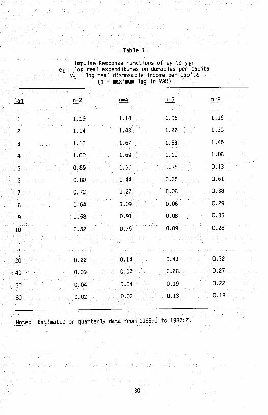
Table 1

Impulse Response Functions of et to yt: et = log real expenditures on durables per capita

= log real disposable income per capita (n = maximum lag in VAR)

n=2 n=4 n=6 n=8

1 1.16 1.14 1.06 1.15

2 1.14 1.43 1.27 1.30

3 1.10 1.67 1.53 1.46

4 1.00 1.69 1.11 1.08

5 0.89 1.60 0.35 0.13

6 0.80 1.44 0.25 0.61

7 0.72 1.27 0.08 0.38

8 0.64 1.09 0.06 0,29

9 0.58 0.91 0.08 0.35

10 0.52 0.75 0.09 0.28

20 0.22 0.14 0.43 0.32

40 0.09 0.07 0.28 0.27

60 0.04 0.04 0.19 0.22

80 0.02 0.02 0.13 0.18

Note: Estimated on quarterly data from 1955:1 to 1987:2.

30

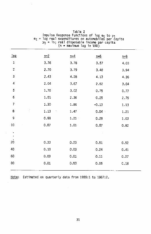
Table 2

Impulse Response Functions of log et to Yt et = log real expenditures on automobiles per capita

Yt = 10; real disposable income per capita (n maximum lag in VAR)

fl fl4 fl 1 3,76 3.78 3.57 4.03

2 2.70 3.79 3,48 3.94

3 2.43 4.28 4.13 4.36

4 2.04 3.67 2.62 3.04

5 1,75 3.02 0.75 0.77

6 1.51 2.36 0,25 2,75

7 1.30 1.86 —0,13 1.13

8 1.13 1.47 0.04 1.21

9 0.99 1.21 0.28 1.03

10 0.87 1.01 0.57 0.82

20 0.33 0.23 0.51 0.52

40 0.10 0.03 0.24 0.41

60 0.03 0.01 0,11 0,27

80 0,01 0.00 0.05 0.18

Note: Estimated on quarterly data from 1955:1 to 1987:2.

31

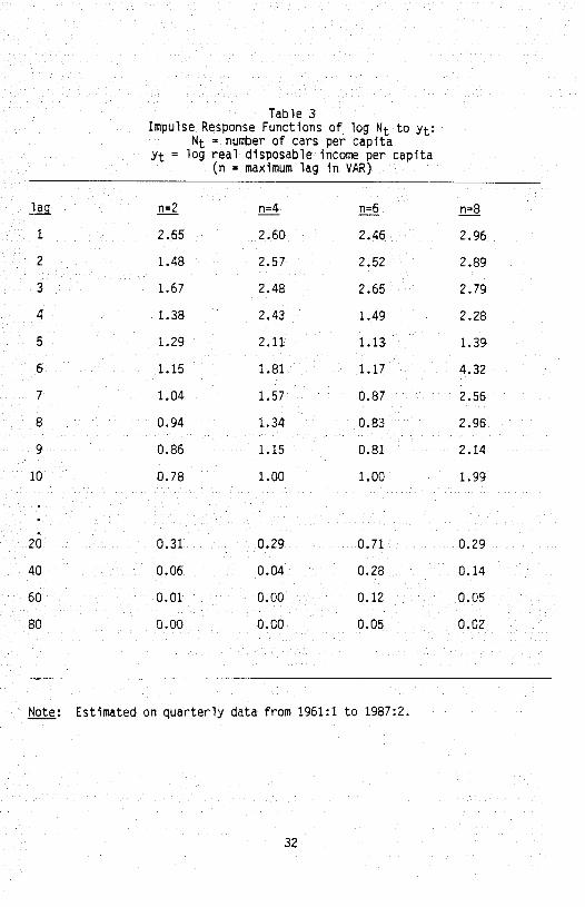
Table 3

Impulse Response Functions of log to yt: Nt = number of cars per capita

Yt = log real disposable income per capita (n = maximum lag in VAR)

1 2.65 2.60 2.46 2.96

2 1.48 2.57 2.52 2.89

3 1.67 2.48 2.65 2.79

4 1.38 2.43 1.49 2.28

5 1.29 2.11 1.13 1.39

6 1.15 1.81 1.17 4.32

7 1.04 1.57 0.87 2.56

8 0.94 1.34 0.83 2.96

9 0.86 1.15 0.81 2.14

10 0.78 1.00 1.00 1.99

20 0.31 0.29 0.71 0.29

40 0.06 0.04 0.28 0.14

60 0.01 0.00 0.12 0.05

80 0.00 0.00 0.05 0.02

Note: Estimated on quarterly data from 1961:1 to 1987:2.

32

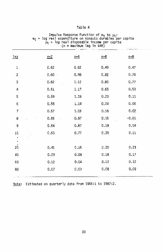
Table 4

Impulse Response Function of et to yt: et = log real expenditure on nonauto durables per capita

Yt = log real disposable income per capita (n = maximum lag in VAR)

n=2 n=4 n=6 n=8

1 0.62 0.62 0.49 0.47

2 0.60 0.98 0.82 0.78

3 0.62 1.12 0.85 0.77

4 0.61 1.17 0.65 0.53

5 0.59 1,18 0.23 0,11

6 0.58 1.14 0.24 0.06

7 0.57 1.06 0.16 0,02

8 0.55 0.97 0.15 -0.01

9 0.54 0.87 0.18 0.04

10 0.53 0.77 0.20 0.11

20 0.41 0.16 0.25 0.23

40 0.23 0.08 0.18 0.17

60 0.12 0.04 0.12 0.12

80 0.07 0.03 0.08 0.09

Note: Estimated on quarterly data from 1955:1 to 1987:2.

33

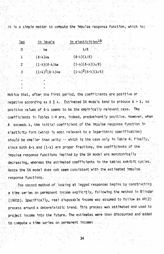
it is a simple matter to compute the Impulse response function, which is:

in levels in elasticities18

0

1 (6-x)x (6-A)(A/6)

2 (1-x)(&-x)x (1-x)(&-A)(x/6)

3 (1—A)2(6—A)X (1—x)2(6—A)(A/6)

Notice that, after the first period, the coefficients are positive or

negative according as & A. Estimated SA models tend to produce 6 > A, so

positive values of &-A seems to be the empirically relevant case. The

coefficients in Tables 1-4 are, indeed, predominantly positive. However, when

6 exceeds A, the initial coefficient of the impulse response function In

elasticity form (which is most relevant to a logarithmic specification)

should be smaller than unity -— which is the case only in Table 4. Finally,

since both 6—A and (1—A) are proper fractions, the coefficients of the

impulse response functions implied by the SA model are monotonically

decreasing, whereas the estimated coefficients in the tables exhibit cycles.

Hence the SA model does not seem consistent with the estimated impulse

response functions.

The second method of looking at lagged responses begins by constructing

a time series on permanent income explicitly, following the method in Blinder

(1981b). Specifically, real disposable income was assumed to follow an AR(2)

process around a deterministic trend. This process was estimated and used to

project Income Into the future. The estimates were then discounted and added

to compute a time series on permanent income:

34

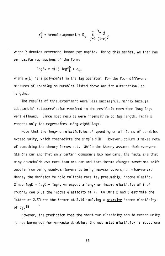
= trend component + Et Z

j=O (1+r)

where Y denotes detrended income per capita. Using this series, we then ran

per capita regressions of the form:

logE = (L) logY +

where (L) is a polynomial in the lag operator, for the four different

measures of spending on durables listed above and for alternative lag

lengths.

The results of this experiment were less successful, mainly because

substantial autocorrelation remained in the residuals even when long lags

were allowed. Since most results were insensitive to lag length, Table 5

reports only the regressions using eight lags.

Note that the long-run elasticities of spending on all forms of durables

exceed unity, which contradicts the simple PIH. However, column 3 makes note

of something the theory leaves out. While the theory assumes that everyone

has one car and that only certain consumers buy new cars, the facts are that

many households own more than one car and that income changes sometimes shift

people from being used—car buyers to being new—car buyers, or vice-versa.

Hence, the decision to hold multiple cars is, presumably, income elastic.

Since logE = logC ÷ logN, we expect a long-run income elasticity of E of

roughly one the income elasticity of N. Columns 2 and 3 estimate the

latter at 2.50 and the former at 2.14 implying a negative income elasticity

of Ct.'9

However, the prediction that the short-run elasticity should exceed unity

is not borne out for non-auto durables; the estimated elasticity is about one

35

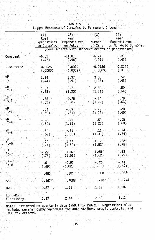
Table 5

Lagged Response of Durables to Permanent Income

(1) (2) (3) (4) Real Real Real

Expenditures Expenditures Number Expenditures on Durables on Autos of Cars on Non-Auto Durables

(coefficients with standard errors in parentheses)

Constant —6.52 -11.01 —6.74 —5.80

(.47) (.96) (.99) (.47)

Time trend 0.0026 -0.0029 -0.0126 0.0044

(.0005) (.0009) (.0009) (.0005)

1.24 3.37 3.06 .52

(.44) (.91) (.92) (.45)

1.03 2.71 2.30 .50

(.63) (1.30) (1.31) (.64)

.38 -0.78 —.74 .78

(.62) (1.28) (1.29) (.63)

.04 —.69 -.72 .28

(.59) (1.21) (1.22) (.60)

-.26 -.75 -.59 —.10 -

(.59) (1.22) (1.23) (.60)

Yt5 —.30 -.31 .11 —.34

(.63) (1.30) (1.31) (.64)

.14 1.44 1.17 —.22

(.74) (1.52) (1.53) (.75)

V -.29 —1.87 —1.68 .13 t

(.78) (1.61) (1.62) (.79)

-.61 -0.97 -.42 -.41

(.49) (1.02) (1.01) (.49)

.980 .881 .808 .983

SSR .1674 .7088 .7187 .1714

0.57 1.11 1.12 0.34

Long—Run Elasticity 1.37 2.14 2.50 1.12

Note: Estimated on quarterly data 1959:1 to 1987:2. Regressions also

included several dummy variables for auto strikes, credit controls, and

1986 tax effects.

36

standard error below one.

The estimates are not particularly favorable to the (S,s) model. But

they should, perhaps, be taken with a grain of salt owing to their poor

statistical properties and to the gross disparities between Table 5 and

Tables 1-4.

5.4 Age Distribution

The model strongly suggests that the age distribution of durables should

affect purchases —— and in a particular way. Specifically (see Figure 5), the

density between s and s1/(1-) governs the number of cars that are purchased. Hence it is neither the stock of the newest cars nor the stock of

oldest cars that should have the greatest influence on new car purchases, but

rather the stock of cars in the age range where new-car buyers tend to trade

in -- say, 1-4 year old cars.

As a test, we obtained annual data on the age distribution of cars in

the U.S. from an industry trade publication.20 These data are based on

automobile registrations at midyear and, given our decision to consider used

cars up to 10 years old, are available back to 1959. Cars are identified by

model year. We grouped them into two—year age bands as follows. Take the data

pertaining to registrations as of midyear 1959 as an example. Cars in the

1959 model year were sold mostly from about September 1958 to about September

1959. Thus, in July 1959, they ranged in age from zero to about nine months

old. We skipped these brand new cars and used, as our youngest vintage, cars

from the 1958 and 1957 model years. These would generally have been between

nine months and 33 months old. As a shorthand, we call these "one and two

year old cars;" in symbols, K2. Proceeding analogously, we defined "three and

year old cars" (K4 ) and so on up to "nine and ten year old cars,"

37

K'1° , which was the oldest vintage we considered. We also, of course, have

data on the total stock of cars irrespective of age, Kt.

The empirical question is: Which version of Kt is the best predictor of

new car purchases, Nt?2' Our theory suggests that K4 or perhaps K2 might do

best while the SA model tacitly assigns declining weights to older vintages.

We used several measures of association. The most naive just compares the

simple correlations between logN and various measures of logK (in per

capita terms). Here K2 and K4 had about equal correlations (in logs)

with Nt (around 0.3), while K8 and K9"° correlated much less well. This is

hardly a precise test, but it leans in the right direction.

Next, we ran causality tests asking whether two lags of each Kt variable

Granger—cause Nt. Unfortunately, there are so few data points that these

tests were almost totally uninformative. (For example, the marginal

significance level for omitting K56 was 0.03 on a 1961-1985 sample, but 0.71

when the sample stopped at 1983.)

Finally, despite our distrust of the model, we ran stock adjustment

equations using alternative measures of the K variable. Here the results were

quite different: the sum of squared residuals was minimized when

(i.e., cars aged 9—10 years) was used as the stock variable.

6. SUP+IARY AND CONCLUSIONS

This paper develops a simple but important point which is often

overlooked by economists: It is quite possible that the best policy for a

rational, optimizing agent Is to do nothing for some period of time——even if

new, relevant, and unexpected information becomes available.

38

We illustrated this point using the market for durable goods. Assuming

that there are lumpy costs in durables transactions, consumers choose a

finite range, not just a single level, for their durables consumption. The

boundaries of this range change with new information and, in particular, have

the homogeneity property we associate with the permanent income hypothesis.

However, as long as the durable stock Is within the chosen region, the

consumer will not change his or her stock. Hence individuals will make

durable transactions infrequently and their consumption might differ

substantially from the prediction of the strict PIH which ignores transaction

costs.

One implication of such microeconomic behavior is that aggregate data

cannot be generated by a representative agent; explicit aggregation is

required. By doing that, we showed that time series of durable expenditures

should be divided to two separate series: One on the average expenditures

per purchase and the other on the number of transactions. The predictions of

the PIH hold for the former, but not for the latter. For example, the

short—run elasticity of the number of purchases with respect to permanent

income is much larger than one for plausible parameter values. The

underlying reason for this large elasticity is that only a fraction of the

population buys a durable each period. A small change in the behavior of the

total population might therefore translate into a large change in the

fraction of consumers who are active in the market in a given period. Hence

the durable goods market is inherently more volatile than the market for

nondurable goods and services.

We put our theory to a battery of empirical tests. Although the tests

are by no means always consistent with the theory, most empirical results are

in line with our predictions. Using tests of the Hall (1978) type, we showed

39

that time series on average expenditures on cars but not the number of cars,

are consistent with the standard predictions of the PIH; short run impulse

responses of car sales to income innovations are significantly larger than

one; variance of the sales series is much larger than both the variance of

the income process and the average transaction size.

This indicates that there may be more than a grain of truth in our

theory, a theory which demonstrates that there is nothing irrational about

consumers' behavior which does not always respond to new, unexpected

information. Failure to realize that might prevent understanding important

macroeconomic phenomena.

40

FOOTNOTES

1. This Is a major point of Grossman and Laroque (1987).

2, Again see Grossman and Laroque or, for a somewhat different specification

based on proportional, rather than fixed, transactions costs, Constantinides

(1986).

3. See Sheshinski and Weiss (1977) or, more recently, Caplin and Spulber

(1987).

4. See Abel (1980).

5. The lemons principle is not the only rationale for a gap between buying

and selling prices. In addition, we have worked out a basically equivalent

iiodel in which the lumpy transactions cost is a loss of utility,

6. Constantinides (1986) argues that proportional transactions costs also

lead to similarly inertial behavior.

7. Again, proportional adjustment costs lead to a somewhat different form of

Inertial behavior; see Caplin and Krishna (1987).

8. The setup and proof of this theorem owes much to the earlier work of

Flemming (1969).

9. As long as t=O is not the first purchase moment, a stronger result holds:

X0, all the S, and all the S, are proportional to W0, that is, two

individuals with different K0 but identical financial wealth choose the same

(S,s) boundaries. (See Figure 3).

10. Readers of Grossman and Laroque (1987) may wonder why we describe their

rule by four parameters while the authors themselves describe it as a

three-parameter rule. The reason is that they collapse our two 5L and Sj

parameters into a single parameter by writing their counterpart to S as

proportional to wealth net of transactions costs. As we have just noted,

transactions costs are larger when you trip the upper boundary than when

41

you trip the lower s boundary; hence wealth net of transactions costs differs

in the two cases.

11. Later we will show that it is easy to generalize to an arbitrary number

of cars, so long as they all depreciate at the same rate.

12. Since we are interested in modelling purchases of new cars, we need only

be concerned with crossings of the lower border, s. An Individual who--say,

because of a drop in permanent income——finds himself above and sells his

late model used car to buy an older one does not affect new car purchases.

13. The data are unpublished arid were kindly furnished by the Bureau of

Economic Analysis. The period of observation is 1959:1 through 1987:2, and

all data are seasonally adjusted. Ct is average expenditure per new car

purchased by consumers, deflated by the PCE deflator. Nt is per capita

retail sales of new passenger cars to consumers (business and government

expenditures are excluded).

14. All regressions also included dummy variables for strikes, the 1980

credit controls, and the tax—induced buying spurt in the second half of 1986.

15. For example, just ending the sample at 1985:4 leads to a marginal

significance level of 0.005 rather than the .14 reported in the text.

16. All regressions include a constant, a time trend, and the dummies

mentioned in footnote 14.

17. See, for example, Campbell and Mankiw (1986).

18. Elasticities are evaluated around the steady-state y/E ratio of 1I(&t).

19. In fact, when estimated freely, this elasticity is strongly negative.

20. MVMA Annual Facts and Figures (Motor Vehicles Manufacturers' Association:

Detroit), various issues.

42

21. For this purpose, we took our quarterly data on auto sales and aggregated

them into years beginning in July of the stated year. That is, the 1959

observation covers sales during the last two quarters of 1959 and the first

two quarters of 1960.

43

REFERENCES

Abel, A. B., "Empirical Investment Equations: An Integrative Framework," in K. Brunner and A. H. Meltzer (eds.), On the State of Macro-economics.

Carnegie—Rochester Series on Public Policy, 1980.

Akerlof, G. A., "The Market for Lemons: Qualitative Uncertainty and the Market Mechanism," Quarterly Journal of Economics, 1970, 84, 488—500.

Akerlof, G. A. and J. L. Yellen, "Can Small Deviations from Rationality Make Significant Differences to Economic Equilibria?", American Economic Review, September 1985, pp. 708-720.

Blinder, A. S., "Retail Inventory Behavior and Business Fluctuations," Brookings Papers on Economic Activity, 2: 1981a, pp. 443—505.

Blinder, A. S., "Temporary Income Taxes and Consumer Spending," Journal of

Political Economy, February 1981b, pp. 26-53.

Campbell, J. V., "Does Saving Anticipate Declining Labor Income? An

Alternative Test of the Permanent Income Hypothesis,' Princeton Univesity, mimeo, August 1986.

Campbell, J. V. and N. G. Mankiw, "Are Output Fluctuations Transitory?", mimeo, September 1986.

Caplin, A. and D. Spulber, "Menu Costs and the Neutrality of Money," Quarterly Journal of Economics, November 1987.

Caplin, A. and K. Krishna, "Simple Dynamic Model of Labor Demand," mimeo, 1987.

Constantinides, G. M., "Capital Market Equilibrium with Transactions

Costs," Journal of Political Economy, Vol. 94, No. 4, August 1986,

pp. 842-862.

Flavin, M. A., "The Adjustment of Consumption to Changing Expectations about

Future Income," Journal of Political Economy, 1981, 89, 974—1009.

Flemming, J. S., "The Utility of Wealth and the Utility of Windfalls," Review of Economic Studies, 1969, 36, 55—66.

Friedman, B. H., "Optimal Expectations and the Extreme Information

Assumptions of 'Rational Expectations' Macromodels," Journal of

Monetary Economics, Vol. 5, No. 1, January 1979, pp. 23—41.

Grossman, S. J. and G. Laroque, "The Demand for Durables and Portfolio

Choice under Uncertainty," mimeo, Princeton University, June 1987.

44

Hall, R. E., 'Stochastic Implications of the Life Cycle—Permanent Income Hypothesis: Theory and Evidence, Journal of Political Economy, 1978. 86, 971-987.

Hayashl, F., "The Permanent Income Hypothesis: Estimation and Testing by Instrumental Variables," Journal of Political Economy, Vol. 90, No, 5, pp. 895-916, October 1982.

Mankiw, N. G., "Hall's Consumption Hypothesis and Durable Goods," Journal of Monetary Economics, 1982, 10, 417-425.

Sargent, T. J., "Estimation of Dynamic Labor Demand Schedules under Rational Expectations," Journal of Political Economy, Vol. 86, No. 6, December 1978, pp. 1009—1044,

Sheshlnski, E. and V. Weiss, "Inflation and Costs of Price Adjustment," Review of Economic Studies, Vol. XLIV (2), June, 1977 pp. 287-303.

Taylor, J. B., "Monetary Policy during a Transition to Rational Expectations," Journal of Political Economy, Vol. 83, No, 5, October 1975, pp. 1009—1021.

45