NBER WORKING PAPER SERIES

BUSINESS-LEVEL EXPECTATIONS AND UNCERTAINTY

Nicholas BloomSteven J. Davis

Lucia FosterBrian Lucking

Scott OhlmacherItay Saporta-Eksten

Working Paper 28259http://www.nber.org/papers/w28259

NATIONAL BUREAU OF ECONOMIC RESEARCH1050 Massachusetts Avenue

Cambridge, MA 02138December 2020

Any opinions and conclusions expressed herein are those of the authors and do not represent the views of the U.S. Census Bureau, Charles River Associates, or the National Bureau of Economic Research. The Census Bureau has reviewed this data product for unauthorized disclosure of confidential information and has approved the disclosure avoidance practices applied to this release. DRB Approval Number(s): CBDRB-FY17-CMS-6039, CBDRB-FY17-CMS-6064, CBDRB-FY18-CMS-6171, CBDRB-FY18-CMS-6207, CBDRB-FY18-CMS-6334, CBDRB-FY18-CMS-6802, CBDRB-FY19-CMS-7201, CBDRB-FY20-CES007-001, CBDRB-FY21-CES007-002. We gratefully acknowledge financial support from the National Science Foundation, the Kauffman Foundation and the Sloan Foundation, with grants administered by the National Bureau of Economic Research. Numerous Census Bureau staff helped develop, conduct and analyze the survey; we especially thank Julius Smith, Marlo Thornton, Cathy Buffington, William Wisniewski, and Michael Freiman. We also thank Mike Bryan, Nick Parker, and Brent Meyer of the Federal Reserve Bank of Atlanta, with whom Bloom and Davis developed and tested firm-level versions of the five-point forecast distribution questions posed to manufacturing plants in the 2015 MOPS. We thank participants at numerous conferences including the 2018 Alabama Economics Association Meeting; 2018 Meetings of the American Economic Association; the Conference on Global Risk, Uncertainty, and Volatility at the Federal Reserve Board of Governors; the 2018 Cowles Foundation Conference on Macroeconomics; the Developing and Using Business Expectations Data Conference at the University of Chicago; the Firm Dynamics and Economic Growth Conference at the Bank of Italy; the 2018 FSRDC Annual Meeting at Penn State University; the 2018 Southern Economic Association Annual Meetings; the 2018 Toulouse Network for Information Technology Annual Meeting; the Uncertainty, Trade, and Firms Workshop at the Research Institute of Economy, Trade, and Industry; as well as participants at seminars at the Center for Economic Studies, Cornell University, the Federal Reserve Board of Governors, the National Economists Club and Society of Government Economists, and Osaka University; Emek Basker, and John Eltinge for helpful comments.

NBER working papers are circulated for discussion and comment purposes. They have not been peer-reviewed or been subject to the review by the NBER Board of Directors that accompanies official NBER publications.

© 2020 by Nicholas Bloom, Steven J. Davis, Lucia Foster, Brian Lucking, Scott Ohlmacher, and Itay Saporta-Eksten. All rights reserved. Short sections of text, not to exceed two paragraphs, may be quoted without explicit permission provided that full credit, including © notice, is given to the source.

Business-Level Expectations and UncertaintyNicholas Bloom, Steven J. Davis, Lucia Foster, Brian Lucking, Scott Ohlmacher, and Itay Saporta-EkstenNBER Working Paper No. 28259December 2020JEL No. L2,M2,O32,O33

ABSTRACT

The Census Bureau’s 2015 Management and Organizational Practices Survey (MOPS) utilized innovative methodology to collect five-point forecast distributions over own future shipments, employment, and capital and materials expenditures for 35,000 U.S. manufacturing plants. First and second moments of these plant-level forecast distributions covary strongly with first and second moments, respectively, of historical outcomes. The first moment of the distribution provides a measure of business’ expectations for future outcomes, while the second moment provides a measure of business’ subjective uncertainty over those outcomes. This subjective uncertainty measure correlates positively with financial risk measures. Drawing on the Annual Survey of Manufactures and the Census of Manufactures for the corresponding realizations, we find that subjective expectations are highly predictive of actual outcomes and, in fact, more predictive than statistical models fit to historical data. When respondents express greater subjective uncertainty about future outcomes at their plants, their forecasts are less accurate. However, managers supply overly precise forecast distributions in that implied confidence intervals for sales growth rates are much narrower than the distribution of actual outcomes. Finally, we develop evidence that greater use of predictive computing and structured management practices at the plant and a more decentralized decision-making process (across plants in the same firm) are associated with better forecast accuracy.

Nicholas BloomStanford UniversityDepartment of Economics579 Serra MallStanford, CA 94305-6072and NBERnbloom@stanford.edu

Steven J. DavisBooth School of BusinessThe University of Chicago5807 South Woodlawn Avenue Chicago, IL 60637and NBERSteven.Davis@ChicagoBooth.edu

Lucia FosterCenter for Economic StudiesCensus BureauRoom 5K032Washington, DC 20233-6300 lucia.s.foster@census.gov

Brian LuckingCharles River Associates601 12th StreetSuite 1500Oakland, CA 94607blucking@crai.com

Scott OhlmacherCensus BureauRoom 5K040BWashington, DC 20233-6300scott.ohlmacher@census.gov

Itay Saporta-EkstenThe Eitan Berglas School of Economics Tel Aviv UniversityP.O.B. 39040Ramat Aviv, Tel Aviv, 6997801itaysap@tauex.tau.ac.il

Managerial and Organizational Practices Survey (MOPS) is available at https://www.census.gov/programs-surveys/mops.html

3

1 Introduction

Keen interest in expectations harkens back at least to Keynes (1936), who stressed the importance

of “animal spirits” for firms and the macroeconomy. Classic contributions by Hayashi (1982) and

Abel and Blanchard (1986) highlight the payoff to modelling business expectations in dynamic

models of investment. Indeed, virtually all modern studies of investment, hiring and R&D under

adjustment costs recognize the importance of expectations in business decision making. Leading

examples include Nickell (1978), Caballero (1999), Chirinko (1993), and Dixit and Pindyck

(1994). Despite their importance, however, we have few direct measures of business-level

expectations for real variables beyond qualitative indicators and point forecasts.1

This paper describes the first results of an ambitious survey of business expectations

conducted as part of the Census Bureau’s Management and Organizational Practices Survey

(MOPS).2 MOPS is the first large-scale survey of management practices in the United States,

covering more than 30,000 plants across more than 10,000 firms. Thus far, it has been conducted

in two waves, primarily asking respondents about their practices in 2010 and 2015.3 The size and

high response rate of the dataset, its coverage of units within a firm, links to other Census data,

and comprehensive coverage of manufacturing industries and regions make it unique. As part of

the 2015 MOPS, we asked eight questions about plant-level expectations of own current-year and

future outcomes for shipments, employment, investment expenditures and expenditures on

materials. The survey questions elicit point estimates for current-year (2016) outcomes and five-

point probability distributions over next-year (2017) outcomes, yielding a much richer and more

detailed dataset on business-level expectations than previous work, and for a much larger sample.

1 Guiso and Parigi (1999) and Bontempi, Golinelli and Parigi (2010) use 3-point probability distributions from a

survey of about 1,000 Italian firms per year from 1994 to 2006, and Masayuki (2013) uses 2-point distributions

from a survey of 294 Japanese firms in 2013. See Bachmann, Elstner, and Sims (2013) and Manski (2018) for

additional discussion and references to previous efforts to measure business and household expectations. For

decades, a principal federal economic indicator collected business subjective forecasts of investment. The Plant and

Equipment Survey (PES) was collected on a quarterly basis by the Bureau of Economic Analysis (or its precursor)

from 1947 to 1988Q2 and by the Census Bureau from 1988Q3 to 1993. In 1993, the PES was replaced by the

Investment Plans Survey, which ran semi-annually until 1996, when it was discontinued for budgetary reasons. In

addition, point forecasts for R&D costs are collected as part of the Business R&D and Innovation Survey conducted

by the Census Bureau and the National Science Foundation’s National Center for Science and Engineering Statistics. 2 MOPS is a joint statistical product between the U.S. Census Bureau and a set of external sponsors and subject matter

experts that includes the authors of this paper. The survey was made possible by the generous provision of over $1

million in research support from the U.S. National Science Foundation, the Kauffman Foundation and the Sloan

Foundation. 3 See the descriptions of MOPS in Bloom, Brynjolfsson, Foster, Jarmin, Saporta-Eksten, and Van Reenen (2013) and

Buffington, Foster, Jarmin, and Ohlmacher (2017).

4

Among plants in the 2015 MOPS publication sample, 85% provide logically sensible

responses to our five-point distribution questions, suggesting that most managers can form and

express detailed subjective probability distributions. The other 15% are plants with lower

productivity and wages, fewer workers, lower shares of managers with bachelor’s degrees, and

lower management practice scores and that are less likely to belong to multinational firms. First

and second moments of plant-level subjective probability distributions covary strongly with first

and second moments, respectively, of historical outcomes, suggesting that our subjective

expectations data are well founded. Aggregating over plants under common ownership, firm-level

subjective uncertainty correlates positively with realized stock-return volatility, option-implied

volatility, and analyst disagreement about the future earnings per share (EPS) for both the parent

firm and the median publicly listed firm in the firm’s industry.

The MOPS is a supplement to the 2015 Annual Survey of Manufactures (ASM), and is

mailed to the physical address of all plants in the ASM mail sample, which is drawn from the

universe of large single-unit manufacturing firms and manufacturing establishments of any size

that belong to multi-unit firms. Each variable for which we elicit forecasts in the MOPS has

realized outcomes in the ASM and the quinquennial Census of Manufactures (CMF). As a result,

we can match the MOPS forecasts to realized outcomes. Using these realized values, we find that

forecasts are highly predictive of outcomes. In fact, they are substantially more predictive than

historical growth rates. We also find that forecast errors rise in magnitude with ex ante subjective

uncertainty. Forecast errors correlate negatively with labor productivity, predictive computing, and

the use of structured management practices at the plant.

The paper proceeds as follows. Section 2 discusses the MOPS sample and measurement of

plant-level expectations. Section 3 reports common shapes for the subjective probability

distributions, assesses whether respondents express sensible probability distributions, and

investigates how the ability to express a sensible distribution relates to plant size and age, plant

performance, and the nature of its management practices. Section 4 examines how moments

derived from the subjective expectations data vary with data observable at the time of the plant’s

response to the survey, past growth and volatility at the plant level, and with widely used proxies

for firm-level uncertainty and volatility. Section 5 presents results concerning the forecasts and

their realizations. Section 6 concludes.

5

2 Measuring Business Expectations and Uncertainty

The first wave of the Management and Organizational Practices Survey (MOPS) went to field in

2011 as a mandatory supplement to the 2010 Annual Survey of Manufacturers (ASM).4 This plant-

level survey contained a range of questions about management and organizational practices plus

some background characteristics (but nothing on expectations). The success of this survey led to a

second MOPS wave as a supplement to the 2015 ASM, which added two new sections, Section C

on “Data and Decision-Making” and Section D on “Uncertainty,” and expanded Section E on

“Background Characteristics.” Section D contained eight questions on plants’ expectations for

2016 and 2017 over four outcomes: shipments, investment expenditures, employment, and

materials expenditures. The MOPS contains a question for “Certification,” where the respondent

designates the “name of [a] person to contact regarding this report” as well as that person’s title.

Based on this certification data, the 2015 MOPS survey was typically answered by senior plant

management, in that the most common position title of the contact name is “plant manager” (13%),

“financial controller” (10%) or “CEO” (6%), with about 90% within broad categories of

“management” or “finance” (see Table A1).

This survey was sent electronically as well as by mail to the physical address of each

establishment, with response mandated by Federal law. Most respondents (80%) completed the

survey electronically, with the remainder completing the survey by paper. Non-respondents were

mailed a follow-up letter after six weeks. A second follow-up letter was mailed if no response had

been received after 12 weeks. The first follow-up letter included a copy of the MOPS instrument.

We start by discussing our two types of measures of expectations. The question for 2016

elicited a point estimate, asking (for example for shipments) “For calendar years 2015 and 2016

what are the approximate values of products shipped, including interplant transfers, exports, and

other receipts at this establishment? Exclude freight and excise taxes.”5 Since the survey was sent

out in April 2016 with collection ending in October 2016, the 2015 figure would have likely been

known, and was requested to provide a benchmark for growth rates. The 2016 figure, however,

would have been a partial-year forecast, as respondents are asked to provide an estimate for the

4 Note that the ASM is a retrospective survey, so the April 2011 survey wave asked about data for calendar year 2010. 5 The language describing the response variables for all eight questions in Section D is identical to the corresponding

questions on the ASM. Definitions of these variables identical to the definitions provided in the ASM instructions

were also provided on a FAQ webpage. https://www.census.gov/programs-surveys/mops/about/faq.html

6

calendar year.

The corresponding question for 2017 asked for the lowest, low, medium, high, and highest

possible outcomes for shipments, as well as for the corresponding probabilities such that they add

to 100%. Since this question is more complex, the survey questionnaire included a vignette (pre-

completed example) to help explain the question. See Figure 1 for the vignette.6 The idea behind

this question is to collect probability distributions over own-plant outcomes. The five-point

structure offers a feasible level of response detail based on multiple rounds of cognitive testing

with the Census Bureau and the Federal Reserve Bank of Atlanta from 2013 to 2015.7 It is also

extremely flexible in that respondents have nine degrees of freedom to characterize their

expectations – five outcomes and five probabilities less one restriction that the probabilities add to

100%.

We chose this two-part structure -- asking first for outcomes distributed over five points

and then asking for the associated probabilities – for a number of reasons. Pre-defined outcome

points (or bins), as in the Survey of Professional Forecasters for macro outcomes, do not yield

adequate spread and granularity across thousands of plants that vary greatly by age, size, and

industry unless we use many, many more points.8 Because annual GDP growth rates for the United

States are highly likely to fall within the between negative three percent and four percent, eight

outcome points can adequately span the relevant range of possibilities with reasonable granularity.

For individual manufacturing plants, however, annual growth rates typically have far larger ranges

(for example, from -50 to 100 percent or more) and the central tendency of likely outcomes differs

greatly over plants. To encompass a range from -50 to 100% with one-point spreads between nodes

would require 151 points. In addition to the practical consideration, we also want to avoid

anchoring or tilting the responses by pre-specifying the support of the subjective probability

distributions. Hence, we instead designed a survey that first let businesses define their own

6 We test for anchoring effects in section 3 below and find 5% or less of respondents provide vignette probabilities

to questions and very few individuals (too few to disclose) provide vignette outcomes. 7 Bloom and Davis worked with a team at the Atlanta Fed to develop a similar survey on a smaller panel of around

1,750 firms to collect monthly expectations data over time, and to provide first and second moment aggregate

indicators to help inform monetary policy. See Altig, Barrero, Bloom, Davis, Meyer, and Parker (2020) for details

about the Atlanta Fed survey, and Bloom, Bunn, Chen, Mizen, Smietanka, and Thwaites (2019) for a similar

application in a Bank of England UK survey. For information on the cognitive testing process for the MOPS, see

Buffington, Herrell, and Ohlmacher (2016). 8 For the Survey of Professional Forecasters, see https://www.philadelphiafed.org/research-and-data/real-time-

center/survey-of-professional-forecasters/.

7

outcome points and then assign probabilities to these points. Moreover, the great flexibility of the

design with five outcomes and five probabilities meant complex expectational distributions could

be captured, avoiding limiting respondents to, for example, normal or triangular probability

distributions.

We create our measures of uncertainty for each MOPS respondent based on each

establishment’s expectations or forecasts. For each of the four measured outcomes (shipments,

employment, materials, and capital), we create a measure of uncertainty about growth rates. For

example, the shipments measure of uncertainty is the standard deviation of the establishment’s

growth rate based on actual shipments in 2015 as reported on the MOPS and the set of five

forecasted values. Specifically, it is measured as the standard deviation of the plant’s predicted

annual growth rates 2015-2017 (over the five points). We measure volatility of historical growth

rates, or the variation over realized values, as the standard deviation of the establishment’s annual

growth rates for all years from 2004-2015, as available.

2.1 Sample and Sample Selection

All plants in the mail sample for the 2015 ASM on January 2, 2016 were mailed a copy of the

2015 MOPS survey instrument and instructions for reporting on April 28, 2016. The instructions

stated that responses were due by June 24. As noted above, two follow-up letters were sent to

potential respondents on an as-needed basis. Collection of responses closed on October 31, 2016.

The MOPS sample was also supplemented in the first follow-up mailing with new plants of multi-

unit firms and newly in-scope manufacturing plants identified from ASM responses.

Of the approximately 50,000 plants in the MOPS mail sample, about 35,000 establishments

returned responses that were considered valid for inclusion in tables published by the U.S. Census

Bureau. In order to be included in this tabulation sample, respondents needed to provide answers

to all seven questions in Section A (questions 1, 2, 6, and 13-16) that could not be skipped

according to the instructions in the survey. The official Unit Response Rate (URR) computed by

the U.S. Census Bureau is the number of respondents divided by the number of respondents who

were either eligible for response or for whom eligibility could not be determined. That is, the

denominator of the URR also includes plants whose forms were returned to the Census Bureau by

the U.S. Postal Service as “Undeliverable as Addressed.” The URR for the 2015 MOPS was

70.9%, compared to 74% for the 2015 ASM. These MOPS respondents accounted for 71.9% of

8

2015 ASM shipments reported by all plants in the MOPS sample.

The MOPS follows an uncommon mail strategy for a Census Bureau survey. For the ASM,

the Census Bureau mails survey forms and instructions to the “business address” associated with

plants in the Business Register (BR). In general, for plants belonging to multi-unit firms, this

means that survey forms are mailed to a central address (often headquarters). In contrast, the

MOPS is mailed directly to the physical address of the plant.9 This mail strategy is pursued because

managers at the physical plant are more likely to have information about plant-level management

practices. Where a contact name for the plant was available in the BR, the form and instructions

for the MOPS were addressed to that name. Otherwise, these packages were mailed attention:

“Plant Manager.” For more technical information on the MOPS sample, collection, and processing,

see Buffington, Hennessy, and Ohlmacher (2017) or https://www.census.gov/programs-

surveys/mops/technical-documentation/methodology.html.

The baseline sample for our analysis is the set of approximately 35,000 respondents to the

2015 MOPS who could be matched to 2015 ASM results and were thus included in the published

MOPS tables. Further sample restrictions are assigned as discussed below according to the

availability of valid responses to the forecasting questions. The forecasting data underwent a

rigorous cleaning process that is detailed in the data appendix.

3 Response Characteristics

In Figure 2, we present the mean of the respondent-provided probabilities for each scenario over

the four measures. This average probability distribution is roughly symmetric and centered on the

medium scenario. Table 1 reports the ten most common subjective probability distributions elicited

by the question on future shipments. Consistent with Figure 2, seven of the top ten most common

distributions (ranks 2, 3, 6-10) are symmetric and centered at the medium scenario. The final row

of the table (“Other”) reports the mean probability distribution of the approximately 60% of

respondents who do not provide one of the top ten most common distributions is also close to

symmetric, with somewhat higher probabilities on the two high scenarios.

9 If a mailing to the physical address of a plant belonging to a multi-unit firm was returned as “Undeliverable as

Addressed,” subsequent follow-up mailings were sent to the business address associated with that plant.

9

About seven percent of all respondents fail to answer the five-point questions about future

shipments, which we interpret as inability or unwillingness to express subjective probability

distributions.10 Rows (2) to (10) report the next nine most common probability distributions. The

vignette is the fourth most common distribution, accounting for five percent of respondents, which

suggests only a mild degree of anchoring. About four percent of respondents report a uniform

probability distribution for future shipments, the fifth most common distribution.

Figure 3 shows that scenario-level outcomes are more dispersed for investment

expenditures than for shipments, employment, or materials expenditures. To construct this figure,

we first express each plant’s scenario-specific forecast values as ratios to its medium-scenario

value for the same outcome variable. Then we compute the mean of these scenario-specific ratios

over plants. For sales, employment, and cost of materials, the mean ratios are about 0.9 for lowest-

to-medium scenarios and less than 1.1 for highest-to-medium scenarios. That is, the typical plant

reports highest-lowest differentials that are approximately 20% of the medium-scenario value of

sales, employment, and materials costs. In contrast, the highest-lowest differential for investment

is more than 65% of the medium-scenario value. This pattern is consistent with lumpy investment

behavior, where investment outcomes potentially differ across scenarios for the typical plant.

Table 2 considers quality indicators for the subjective expectation responses to the

questions about future shipments. It also considers how response quality and other characteristics

of the subjective distributions vary with selected plant characteristics. We regard three conditions

as minimal requirements for a “good response” to our questions about subjective expectations.

First, 90% of plants report probabilities that sum to a value between 90 and 110%.11 Second, 97%

report a distribution with at least two mass points. Third, 85% report future shipments that rise in

a weakly monotonic manner over the five points from Lowest to Highest. Perhaps surprisingly,

85% of respondents express subjective probability distributions over future shipments that meet

all three requirements for a “good response.” Similar results hold for questions about subjective

expectations over employment, capital, and materials expenses. This pattern of results says that

management at most plants can form and express coherent probability distributions in response to

10 Those leaving these responses blank did typically complete prior and subsequent questions (and were required to

have provided sufficient responses to Section A for inclusion in the sample), so they are not simply skipping the

entire survey. 11 If respondents round at the cell level, their reported probabilities need not sum to exactly 100%. In practice, very

few respondents supply probabilities that lie within 90% to 110% but do not sum to exactly 100%.

10

our five-point questions. We think this pattern suggests that our subjective expectations data can

provide useful inputs into dynamic models whereby current business decisions depend partly on

expectations about future outcomes, as in models that involve Bellman equations.

Columns (2) to (6) in Table 2 report OLS regressions coefficients of the indicated

distributional characteristic on the plant characteristics. We see that an ability to express “good”

subjective probability distributions is associated with higher management scores as measured by

Bloom, Brynjolfsson, Foster, Jarmin, Patnaik, Saporta-Eksten, and Van Reenen (2019).

Apparently, plants that adopt more structured management practices around monitoring

performance and incentives also have managers that are more able to provide coherent probability

distributions. Good responses are also associated with greater size as measured by employment,

higher earnings per worker, a larger fraction of managers with a college education, and a higher

incidence of multinational ownership. The same pattern holds for each of the individual response

quality indicators as well, confirming our interpretation of the response quality indicators.

Furthermore, failing to provide a forecast of any kind is associated with less-structured

management practices, smaller plant size, lower earnings per worker, and lower shares of

managers with a bachelor’s degree. These results also prompt the hypothesis that an ability to form

and express coherent subjective probability distributions is a signal of management quality, which

produces better plant-level outcomes.

The last six rows consider other aspects of the subjective probability distributions and their

empirical relationship to the plant characteristics. Subjective probability distributions where the

largest probability is assigned to a scenario other than the lowest or highest scenarios (“Interior

mode”) are associated with more structured management practices, greater employment, higher

earnings per worker, greater managerial education, and higher incidence of multinational

ownership. Results are similar for subjective distributions with a single mode, centered mode, non-

uniform distributions and, in attenuated form, for symmetric distributions. Anchoring to the

vignette distribution is also associated with lower earnings per worker, lower shares of managers

with bachelor’s degrees, and lower incidence of multinational ownership. These results suggest

that better performing plants are more likely to provide the “regular” sorts of distributions that we

usually see in actual outcomes for plants, firms and industries.

In summary, Tables 1 and 2 demonstrate that, first, a high percentage of plants provide

11

well-formed five-point probability distributions, suggesting more complex models of economic

behavior involving the formation of expectations across future states are not implausible for plants.

Second, those plants that are unable to provide these probability distributions are not randomly

selected. Instead, they appear to be significantly worse on several performance metrics.

4 Response Quality and Data Validation

In this section we validate the quality of the expectations data by showing that our expectations

and subjective uncertainty measures are highly correlated with observables that one would expect

to be indicative of plant expectations. First, we demonstrate the tight link between subjective

expectations and uncertainty and historical realizations. We then show that our subjective

uncertainty measures are highly correlated with uncertainty measures typically used in the

literature.

4.1 Subjective Uncertainty and Past Realizations

We start with a simple scatterplot of expectations against historical growth for shipments. Figure

4 presents this relationship graphically as a binned scatterplot where it is clear there is a positive

relationship. We then regress the first moment of plant expectations of the growth in shipments,

investment, employment, and materials expenditures on realized growth rates in the prior year.

Results are presented in columns (1)-(4) of Table 3. Column (1) shows that a plant’s expected

growth in shipments from 2015 (using reported shipments from the 2015 MOPS) to 2017 is

extremely correlated (significant at the 1% confidence level) with its shipments growth rate from

2014 to 2015 (using reported sales from the 2014 and 2015 ASM). A one standard deviation

increase in 2014-2015 shipments growth is associated with approximately a two percentage-point

increase in predicted 2015-2017 shipments growth.

Conversely, column (2) of Table 3 shows that expected investment growth from 2015 to

2017 is highly negatively correlated with investment growth between 2014 and 2015. A one

standard deviation increase in 2015-2015 capital expenditure is associated with approximately an

eight percentage-point decrease in the predicted rate of capital expenditure over 2015-2017. This

is likely due to plants making lumpy capital investments such that those that made capital

investments in the previous year are less likely to do so in the immediate future (see Cooper and

Haltiwanger, 2006).

12

Employment and materials growth expectations are similar to shipments growth

expectations – expected employment growth is positively correlated with past employment growth

(column 3), and expected materials-expenditures growth (column 4) is positively correlated with

past growth in materials expenditures. Columns (5) through (8) regress expected growth measures

on all four realized prior-year growth rates simultaneously. Prior shipments, investment, and

employment growth are each strong predictors of plant mean expectations, while prior materials

expenditures growth does not appear predictive of expectations conditional on the other realized

growth measures, likely due to a high degree of correlation between materials cost and shipments.

We also looked at longer run measures of growth – for example, shipments growth from 2012 to

2015 – and found very similar results.

Table 4 conducts an analysis similar to the one in Table 3 for the second moments, i.e., a

measure of uncertainty, of plant expectations and past performance. We construct measures of

plant historical shipments (investment, employment, materials) growth volatility by taking the log

standard deviation of every realization of annual plant growth in shipments (investment,

employment, materials) from 2004 through 2015, as available. Only plants with at least five

observations on historical growth rates are kept, somewhat shrinking the sample size.12 Columns

(1) through (4) show that a plant’s historical realized volatility is highly positively correlated with

the log of our measure of subjective uncertainty over future growth rates (standard deviation in the

growth rates forecast for 2017). This is also shown for shipments in Figure 5, where we see an

extremely strong and monotone upwards sloping relationship between historical shipments

volatility and subjective shipments uncertainty. This is a striking result: a plant’s subjective

uncertainty over future sales growth is tightly related to its historical volatility of sales growth,

indicating the second-moment variations in these expectations are informative. The magnitude of

this relationship is substantial. A one standard deviation increase historical volatility of shipments

growth is associated with a 15.6 log-point increase in the subjective uncertainty measure. On the

other hand, there seems to be considerable variation in the subjective uncertainty measure that is

not explained by historical volatility. The informational power of that additional variation will be

explored in future work.

12 This inclusion criterion means that plants have to be included in at least two prior ASM survey waves. Because

larger plants have a higher probability of being included in each ASM survey wave, this oversamples larger plants.

13

In Table 4 columns (5) through (8) we include all the historical volatility measures

simultaneously. For example, column (5) regresses shipments growth uncertainty on realized

shipments, investment, employment, and materials growth volatility. Each of the measures is a

strong predictor of subjective uncertainty. However, comparing the t-statistics for each

independent variable it is clear that past shipments growth volatility is the most significant

predictor of future shipments growth uncertainty. The same is true for the other outcomes we

measure – in columns (6) through (8) the most significant predictor of uncertainty with respect to

each outcome is past volatility of that outcome. While these regressions are not causal, this pattern

highlights how plant-level subjective uncertainty varies across outcomes in line with their

historical experiences – for example, plants with historically highly volatile shipments but stable

employment report relatively greater subjective uncertainty for shipments as compared to

employment.

The fact that uncertainty over each outcome is most correlated with that outcome’s past

volatility suggests that there is a great deal of informational content in the subjective expectations

data. In particular, it suggests that there is independent information about plant subjective

uncertainty in each of the solicited expectations distributions. In Table A2, we provide further

evidence of this by showing the pairwise correlations of the first and second moments of the

forecast distributions for each outcome variable. Although the moments are correlated across

outcome variables, the correlation is by no means close to one – for example the second moment

of shipments and materials cost have the highest correlation of 0.59 compared to a correlation of

0.26 between the second moments of shipments and investment – so there is quite a bit of

independent variation in the expectations over each outcome.

In the final column of Table 4, we add measures of firm and industry realized volatility to

the regression of shipments growth uncertainty on plant realized volatility. Conditional on the

plant’s own history of shipments growth volatility, historical volatility of other plants in the same

firm and of other plants in the same industry are both strongly positively correlated with plant

subjective uncertainty. In unreported regressions we show that results for uncertainty over

investment, employment, and materials growth are similar.

Summarizing the results in Tables 3 and 4, the expectations data provided by MOPS plants

is strongly correlated with historical realizations. Historically faster-growing plants report higher

14

mean expected future growth rates, and plants with more volatile histories report more disperse

expected future growth rates. This is an important validation of the quality of the expectations data.

The fact that expectations are strongly correlated to observables which, a priori, seem likely to

influence expectations suggests that the information provided is high quality in the sense that

plants are taking the survey seriously and providing thoughtful responses to the expectations

questions.

Finally, we run validation tests on the relationships between uncertainty and firm and plant

size, age, and recent shocks, finding reassuring results. Figure 6 shows shipments and employment

uncertainty are declining in firm and plant age and size. Larger, older plants report more

predictable future sales and employment growth. We also examine the relationship between

subjective uncertainty and recent shocks to growth. We proxy shocks to growth as deviations from

long run trends, by taking the difference between prior year shipments growth and the mean of the

plant annual shipments growth over the period 2004-2015. Figure 7 plots the relationship between

subjective uncertainty and these growth “shocks.” We observe a v-shaped relationship between

subjective uncertainty and shipments growth deviations from trend. The relationship is centered at

zero. Plants that experienced shipments growth in 2014-2015 close to their historical mean growth

report the least subjective uncertainty, but as the prior year’s growth deviates from the historical

mean, either positively or negatively, uncertainty rises.13

4.2 Subjective Uncertainty Correlates with Commonly Used Measures

In Table 5 we show that the measures of firm uncertainty commonly used in the literature are

strongly correlated with our subjective uncertainty data, justifying the widespread use of these as

proxies for subjective uncertainty. The three firm-specific proxies for uncertainty which we

consider are (a) realized stock returns volatility, (b) options-implied volatility, and (c) forecaster

disagreement. For this analysis, we aggregate Census data to the firm level by taking the

employment-weighted mean of the plant-level log subjective uncertainty, defined as the standard

deviation of the plant’s subjective forecast distribution over its annualized growth rate from 2015

to 2017. We then match these measures to stock market data on publicly-listed firms, which yields

13 Using German data, Bachmann, Carstensen, Lautenbacher, and Schneider (2018) find a similar v-shaped relation

between temporal changes and subjective uncertainty.

15

a sample of approximately 750 firms with approximately 5,100 underlying plants.

In column (1) of Table 5 we regress firm subjective shipments-growth uncertainty on the

log standard deviation of daily stock returns of the firm over the prior year (2014). Daily stock

returns are a common measure of firm uncertainty, used by dozens of papers, for example Leahy

and Whited (1996) and Bloom, Bond, and Van Reenen (2007). Similar to Table 4, we find there

is a strong positive relationship between the financial volatility in 2014 and uncertainty over 2015-

2017 shipments growth. Although the relationship is not necessarily causal, we find that a 10%

increase in realized firm stock-market volatility in 2014 is associated with a 2.71% increase in firm

subjective uncertainty over shipments growth from 2015 to 2017. That is, firms with more recent

financial volatility are less certain about future outcomes.

In columns (2) and (3) we conduct the analysis at the industry-level by regressing firm

uncertainty on the median log standard deviation of daily stock returns in 2014 for the firms within

the same industry. Since this specification does not require us to match to firm-specific data on

publicly listed firms, the sample in column (2) is the full sample of firms with plants which had

good expectations data for all four outcomes. Even at this more aggregate level, there is a strong

relationship between industry-specific stock market volatility and subjective uncertainty

(significant at 1% level). This suggests industry level stock-volatility can provide a good proxy for

the uncertainty in both public and private firms in the same industry. The industry proxies allow

us to verify that the relation between subjective uncertainty and realized volatility is similar for

privately held firms, for which we do not have firm-level stock data.

Columns (4) through (11) show that the strong link with subjective uncertainty is

maintained when using other commonly used uncertainty measures including options-implied

volatility (used for example by Paddock, Siegel, and Smith (1988), Bloom (2009), and Kellogg

(2014)); forecaster disagreement (see for example Bachmann, Elstner, and Sims (2013), Bond and

Cummins (2004), and Xiao (2016)); and dispersion of stock returns among firms in the same

industry.14 For both options-implied volatility and forecaster disagreement, the measures of

financial risk are captured for 2016, contemporaneously with the collection period for the MOPS

survey. In columns (4) through (9), we find that present risk as measured by financial markets is

14 See, for example, the survey of measures of uncertainty in Bloom (2014).

16

correlated with the firms’ own subjective uncertainty.

5 Forecasts Bias and Productivity

Thus far, we considered expectations with historical data and business characteristics. We now

combine expectations and realizations. We use the 2017 Census of Manufactures (CMF) to

investigate the predictive power of forecasts in Section 5.1. In Section 5.2 we evaluate average

bias of the forecasts and demonstrate that bias and forecast accuracy are systematically linked to

plant characteristics. Finally, in Section 5.3 we show that forecast errors and especially over-

optimism correlate with low measured realizations of productivity.

5.1 Predictive Power of Forecasts

We start with a graphical representation of the relation between expectations and realizations.

Figure 8 plots the expected shipments growth on the x-axis and realized shipments growth on the

y-axis. Expected growth is measured using the 2015 value from the MOPS and the 2017 forecast

from the MOPS. In contrast, the realized growth rate is measured using the ASM (2015) and CMF

(2017). Each dot on the plot is the mean of approximately 500 plants. The plot shows a clear

positive relationship, which suggests that forecasts are strongly predictive of outcomes.

In Table 6, we explore the predictive power of the 2015-2017 shipments growth forecasts

provided by respondents, by regressing realized on forecasted shipments growth. In column (1)

we see that forecasts are highly predictive of realized growth (t-stat of over 27). As we add

historical shipments growth (column 2), historical employment and investment growth (column

3), and other controls to the regression (column 4), the coefficient on the forecast remains stable

and significant. Furthermore, we observe that the plant’s forecast in column (1) accounts for nearly

twice the variation in realized growth when compared with a regression of other controls without

the forecast variable, as reported in column (5).

Although we have shown that forecasts are highly predictive, estimates of the magnitude of

the relationship between expected and realized growth might still be attenuated towards zero by

measurement error. The MOPS design allows us to construct a proxy measure for reporting

accuracy, as the average difference between reported 2015 values of shipments and employment

on the MOPS versus the values of the same variables reported on the 2015 ASM. The smaller this

17

difference is, the more likely that the MOPS response is accurate. In column (6), we weight the

regression from column (1) using the inverse of this measurement-error proxy. When we weight

the regression using a measure of reporting accuracy, the coefficient on the shipments forecast is

not statistically different from one and the R-squared of the regression increases as well. That is,

when we account for measurement error, there is nearly a one-to-one relationship between

forecasts and realizations.

We have established that there is a tight relation between the first moment of expectations

and realizations. Our data allow us to evaluate the second-moment relation as well. Defining the

expectation error as the difference between expected and realized growth over the 2015-2017

horizon, we can ask whether plants that exhibit higher subjective uncertainty make larger errors in

their predictions. In Figure 9, we see that the magnitude of the expectation error, measured as the

absolute value of difference between expected and realized 2015-2017 shipments growth, is

increasing in the plant’s subjective uncertainty. This is a striking relationship: plants that provide

more dispersed forecasts have significantly larger expectation errors in absolute value. Figure 10

inverts the analysis in Figure 9, allowing us to study whether or not high levels of (ex-ante)

subjective uncertainty relate differently to positive errors (over-optimism) versus negative errors

(over-pessimism). Consistent with the results in Figure 9, plants with small expectations errors

tend to have been more certain in their forecasts. Those with larger positive or negative expectation

errors gave forecasts with higher uncertainty. To summarize, high subjective uncertainty is highly

predictive of ex-post inaccurate forecasts, and the relation between expectation errors and

subjective uncertainty seems to be roughly symmetric.

5.2 Forecast Bias and Accuracy

Table 7 starts by comparing the first and second moments of the shipment forecast to the realized

outcomes. We see in the first row that plants forecasted a growth rate of 2.8% on average between

2015-2017, but the realization was -0.17%. This appears to imply plants are “over optimistic,”

since their forecasted sales growth rate is above the actual realized sales growth rate. However,

this forecast was potentially reasonable given that the annual growth of US manufacturing output

from 2010 to 2014 was 2.7%, and manufacturing output growth fell to -0.1% during the years 2015

18

to 2017.15 So, while this positive forecast error could imply plants are over optimistic, it could also

be due to an unexpected slowdown in US manufacturing between 2015 and 2017. In the second

row of Table 7, we compare plants’ subjective uncertainty with the forecast bias, and find the

standard deviation of the bias is four times the forecast value. This implies plants are “over precise”

in their forecasts in that they provide confidence intervals for sales growth that are more narrow

than the realized spread of forecast bias. This result is entirely consistent with a long psychology

literature on the tendency of individual to provide “too precise” forecasts.16 So, in summary, plant

forecasts appear approximately correct in levels (they are neither overly optimistic nor overly

pessimistic), but have too narrow upper and lower bounds (they are over-precise).

Table 8 examines the mean squared error (MSE) of the 2015-2017 shipments growth

expectation error. Each pair of columns in Table 8 splits the sample by one plant characteristic.

We split the sample into the top and bottom 50% according to each variable, after removing

industry means. Panel A of Table 8 shows that in the MSE sense, expectation errors are lower for

plants with more structured management practices (columns 2-3), more intensive use of predictive

computing (columns 4-5), and those that are part of more decentralized firms (columns 6-7).

Columns 8-9 shows that the MSE of plants that are above the median over all three of these

characteristics is roughly 40% lower than the MSE of plants that are below the median on all of

these characteristics. Plants that utilize more structured management practices and more predictive

computing and are part of less centralized firms are more accurate in their predictions of future

outcomes than plants that exhibit none of these characteristics.

In the second panel of Table 8, we repeat the comparison exercise for the average

expectation bias instead of MSE. Biases are generally smaller for plants with more structured

management practices, more intensive use of predictive computing, and that are part of more

decentralized firms. However, differences are small and not always significant. We find similar

results for over-extrapolation bias in Panel C. Interestingly, for plants that rank above median on

all three dimensions (column 8), we do not find significant evidence for over-extrapolation.

Table 9 analyzes the relationship between forecast errors and plant practices in regression

format, allowing us to control for other plant characteristics. We regress the square expectation

15 Annualized growth of real manufacturing sector output sourced from https://fred.stlouisfed.org/series/OUTMS#0. 16 See also the results and discussion in Barrero (2020).

19

error (the difference between expected and realized 2015-2017 growth rate of shipments) on

dummy variables for plant characteristics being below median. Consistent with the results in Table

8, columns (1) and (2) show that errors are larger for plants with low structured management

scores, low use of predictive computing, and that have more centralized decision rights. Column

(3) adds three important plant characteristics. Low salaries per worker, one possible proxy for

worker skill, are associated with high errors and less accurate forecasting, while plant size is only

very weakly related to accuracy. Finally, one hypothesis is that larger expectation errors are driven

by higher volatility of business, which is also correlated with management, computing, and

decentralization. To control for this confounding factor, we also include a measure for the

historical volatility of the establishment shipments growth in column (3). Indeed, this variable is

highly significant, with high volatility establishments showing larger errors. In the presence of

these additional controls, the coefficients on management, computerization, and decentralization

remain positive, though the latter becomes insignificant.

5.3 Forecast Accuracy and Productivity

Although we have not established a causal link, the evidence in Tables 8 and 9 discussed above is

consistent with the idea that business choices of specific organizational practices could affect

forecasting accuracy. Moreover, some business investments are directly aimed at improving

analytical tools and forecasting ability. It is then natural to ask whether improved accuracy affects

business performance. We touch upon this question by looking at the correlation between forecast

accuracy for shipments growth between 2015 and 2017 and the realization of revenue-based labor

productivity in 2017, defined as value added divided by employment.

There are at least three channels through which forecast accuracy can affect revenue

productivity. First, suppose that the business chooses some inputs with partial information about

demand, and that these inputs cannot be adjusted. In that case, poor forecasting implies sub-optimal

input choices. Such sub-optimal choice of inputs could lead to an asymmetric effect on measured

revenue productivity – optimistic plants would over-accumulate inputs, driving down marginal

revenue product, while the opposite relationship would hold for pessimistic plants. Second, if the

plant incurs costs to adjust inputs when new information arrives, then marginal revenue product

could decrease with the size of positive or negative forecast errors. Tanaka, Bloom, David, and

Koga (2019) discuss these two channels at length. Third, suppose that a plant must allocate inputs

20

across multiple product lines, again with limited possibility for adjustment. With inaccurate

forecasts, the plant might end up inefficiently allocating resources, resulting in decreased overall

productivity (see for example Olley and Pakes (1996)).

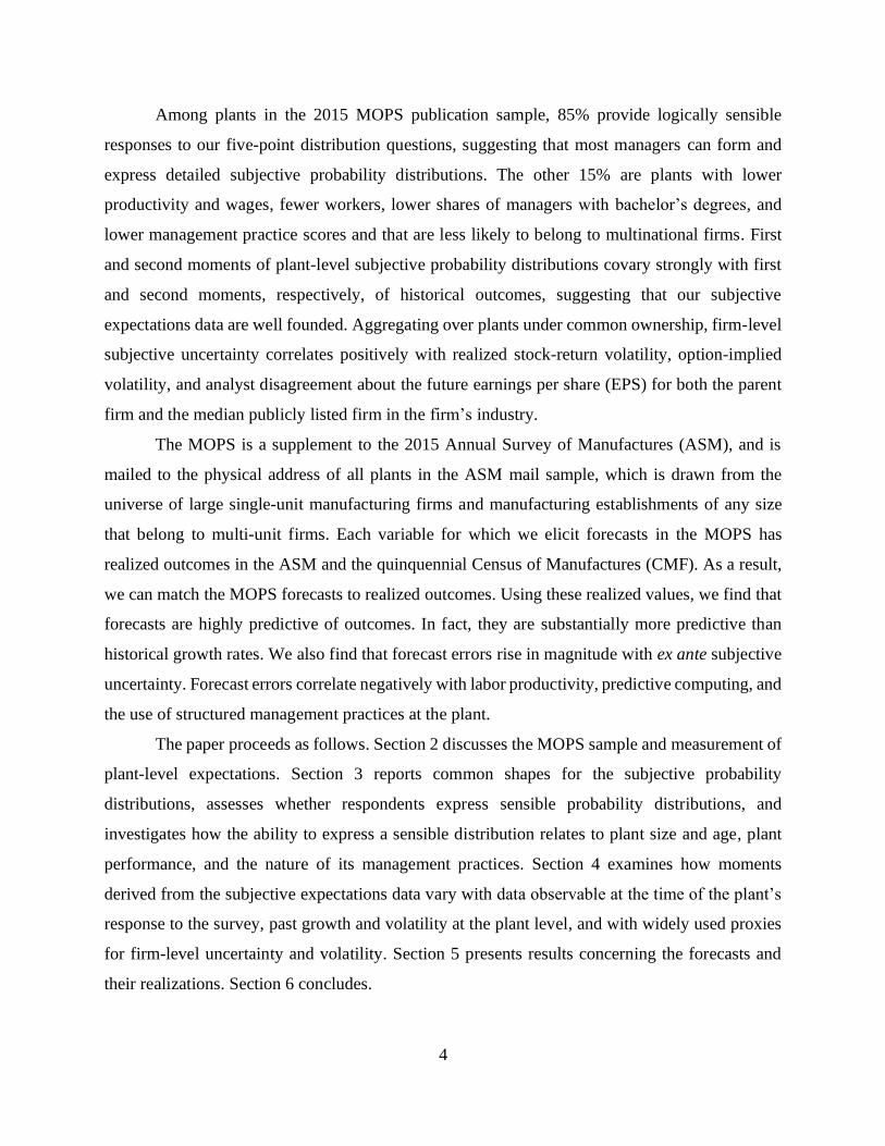
In Table 10, we examine the relationship between expectation errors and labor productivity.

We find that the square of expectation errors for the 2015-2017 growth rate of shipments are

negatively related to labor productivity at the plant level in 2017. This relationship is meaningful;

considering the regression estimate from column (1), and the descriptive statistics in the bottom

panel of Table A3, a one standard deviation increase in the squared expectation error is associated

with approximately 4 log points lower labor productivity, about 5% of a standard deviation. The

relation holds and becomes stronger as we add industry-level fixed effects and survey noise

controls in columns (2) and (3). Column (4) shows that the relation holds even across plants within

the same firm.

One caveat with the analysis in columns (1) through (4) is that the measurement of 2017

shipments in the CMF is used both in the calculation of labor productivity on the left-hand side of

the regression, and in the calculation of the squared expectation error on the right-hand side. If

there is some measurement error in this variable, such measurement error could cause spurious

correlation between the left- and right-hand variables. To alleviate concerns that this is driving the

results, in column (5) we repeat the specification from column (3), instrumenting for the 2015-

2017 squared expectation error using the squared expectation error for the 2015-2016 shipments

growth. We assume that measurement errors within plants across ASM survey waves uncorrelated,

but expectation errors for these two time horizons, both of which rely on expectations reported on

the 2015 MOPS, are correlated. The first-stage indicates that the expectations errors over 2015-

2016 shipments growth are highly correlated with errors over 2015-2017 shipments growth, and

the coefficients of the second-stage IV regression are larger and statistically significant than the

coefficients of the OLS regression.

Finally, as discussed above, we might expect an asymmetric effect with more negative relation

for positive expectation errors (optimism). In column (6), we repeat the specification from column

(5) interacting the squared error with the sign of the error. We find that positive errors are much

more negatively related to labor productivity than negative errors. That is, plants that are overly

optimistic about shipments growth face penalties in terms of realized productivity that are nearly

21

ten times the than plants that are overly pessimistic do. A one standard deviation increase in the

forecast error is associated with a nearly 20 log-point decline in productivity if the error is one of

over-optimism versus a two log-point penalty for an increase in pessimism of the same magnitude.

Figure 11 corroborates these results graphically. To avoid spurious correlation due to measurement

error as discussed above, the figure shows the reduced form corresponding to column (6), i.e. the

relation between 2017 labor productivity and expectation error for the 2015-2016 shipments

growth.

6 Conclusion

The 2015 MOPS, fielded as a partnership between the U.S. Census Bureau and external

researchers, includes innovative questions that elicit five-point probability distributions over future

plant-level shipments, employment, capital expenditures, and expenditures on materials. About

85% of the respondents at 35,000 manufacturing plants provide sensible forecast distributions. The

other 15% are at plants with lower management scores, fewer employees, lower productivity, less

educated managers, and lower multinational ownership.

First and second moments of the plant-level forecast distributions covary strongly with first

and second moments, respectively, of historical outcomes. Firm-level second moments correlate

positively with stock return volatility and analyst disagreement about future earnings per share.

We also find that first moments of subjective forecast distributions are highly predictive of actual

outcomes and, in fact, more predictive than statistical models fit to historical data. When

respondents express greater subjective uncertainty about future outcomes at their plants, their

forecasts are less accurate. However, managers also supply overly precise forecast distributions in

the sense that implied confidence intervals for, say, sales growth rates are much narrower than the

distribution of actual outcomes. Finally, we develop evidence that greater use of predictive

computing and structured management practices at the plant and a more decentralized decision-

making process (across plants in the same firm) are associated with better forecast accuracy.

The MOPS forecast distributions fill a major gap in the Federal statistical system by

providing a rich source of forward-looking information on plant-level and firm-level outcomes. At

one time, the BEA and the Census Bureau collected business-level expectations for investment

expenditures, and the data were widely used. Those collection efforts ended in the 1990s due to

22

budgetary concerns. We expand on those earlier efforts by collecting forward-looking data for

sales, employment, and materials expenditures as well as investment expenditures. Moreover, the

MOPS measures are more sophisticated than their Census and BEA predecessors were, making it

feasible to create uncertainty and tail-risk measures. Our experience collecting subjective forecast

distributions in the MOPS may lead to other efforts to collect business-level expectations.

Currently, we are developing content for another MOPS collection. Expectations data from past

and future MOPS waves will be available to qualified researchers on approved projects in the

FSRDC. We hope others will also use these data to further our understanding of business

expectations and uncertainty, particularly how those concepts relate to businesses decisions and

performance.

23

Bibliography

Abel, Andrew B. and Olivier J. Blanchard (1986), “The Present Value of Profits and Cyclical

Movements in Investment,” Econometrica, 54(2), pp. 249-273.

Altig, David, Jose Maria Barrero, Nicholas Bloom, Steven J. Davis, Brent H. Meyer, and Nicholas

Parker (2020). “Surveying Business Uncertainty,” Journal of Econometrics (Forthcoming).

Bachmann, Rüdiger, Steffen Elstner, and Eric R. Sims (2013), “Uncertainty and Economic

Activity: Evidence from Business Survey Data,” American Economic Journal:

Macroeconomics, 5(2), pp. 217-249.

Bachmann, Rüdiger, Kai Carstensen, Stefan Lautenbacher, and Martin Schneider

(2018). “Uncertainty and Change: Survey Evidence of Firms’ Subjective Beliefs,” University

of Notre Dame mimeo.

Barrero, Jose Maria (2020). “The Micro and Macro of Managerial Beliefs,” ITAM mimeo.

Bloom, Nicholas, Erik Brynjolfsson, Lucia Foster, Ron Jarmin, Megha Patnaik, Itay Saporta-

Eksten, and John Van Reenen (2019). “What Drives Differences in Management

Practices?” American Economic Review, 109(5), pp. 1648-1683.

Bloom, Nicholas, Erik Brynjolfsson, Lucia Foster, Ron Jarmin, Itay Saporta-Eksten, and John Van

Reenen (2013). “Management in America,” Center for Economic Studies Working Paper 13-

01, U.S. Census Bureau.

Bloom, Nicholas, Stephen Bond, and John Van Reenen (2007). “Uncertainty and Investment

Dynamics,” Review of Economic Studies, 74(2), pp. 391-415.

Bloom, Nicholas (2009). “The Impact of Uncertainty Shocks,” Econometrica, 77(3), pp. 623-685.

Bloom, Nicholas (2014), “Fluctuations in Uncertainty,” Journal of Economic Perspectives, 28(2),

pp. 153-176.

Bloom, Nicholas, Philip Bunn, Scarlet Chen, Paul Mizen, Pawel Smietanka, and Gregory Thwaites

(2019). “The Impact of Brexit on UK Firms,” NBER Working Paper 26218.

Bond, Stephen R. and Jason G. Cummins (2004). “Uncertainty and Investment: An Empirical

Investigation Using Data on Analysts Profit Forecasts,” Finance and Economics Discussion

Series 2004-20, Board of Governors of the Federal Reserve System.

Bontempi, Maria Elena, Roberto Golinelli, and Giuseppe Parigi (2010). “Why Demand

Uncertainty Curbs Investment: Evidence from a Panel of Italian Manufacturing Firms,”

Journal of Macroeconomics, 32(1), pp. 218-238.

Buffington, Catherine, Lucia Foster, Ron Jarmin, and Scott Ohlmacher (2017). “The

Management and Organizational Practices Survey (MOPS): An Overview,” Journal of

24

Economic and Social Measurement, 42(1), pp. 1-26.

Buffington, Catherine, Andrew Hennessy, and Scott Ohlmacher (2017), “The Management and

Organizational Practices Survey (MOPS): Collection and Processing,” Center for Economic

Studies Working Paper 18-51, U.S. Census Bureau.

Buffington, Catherine, Kenny Herrell, and Scott Ohlmacher (2016), “The Management and

Organizational Practices Survey (MOPS): Cognitive Testing,” Center for Economic Studies

Working Paper 16-53, U.S. Census Bureau.

Caballero, Ricardo J. (1999). “Aggregate Investment,” in J.B. Taylor and M. Woodford (eds.),

Handbook of Macroeconomics, Volume 1, pp. 813-862.

Chirinko, Robert S. (1993). “Business Fixed Investment Spending: Modelling Strategies,

Empirical Results and Policy Implications,” Journal of Economic Literature, 31(4), 1875-

1911.

Cooper, Russell and John Haltiwanger (2006). “On the Nature of Capital Adjustment Costs,”

Review of Economic Studies, 73(3), pp. 611-633.

Dixit, Avinash K. and Robert S. Pindyck (1994). Investment Under Uncertainty, Princeton:

Princeton University Press.

Guiso, Luigi and Guiseppi Parigi (1999). “Investment and Demand Uncertainty,” The Quarterly

Journal of Economics, 114(1), pp. 185-227.

Hayashi, Fumio (1982). “Tobin’s Marginal Q and Average Q: A Neoclassical Interpretation,”

Econometrica, 50(1), pp. 213-224.

Kellogg, Ryan (2014). “The Effect of Uncertainty on Investment: Evidence from Texas Oil

Drilling,” American Economic Review, 104(6), pp 1698-1734.

Keynes, John M. (1936). The General Theory of Employment, Interest and Money, London:

Macmillan, pp. 161-162.

Leahy, John V. and Toni M. Whited (1996). “The Effect of Uncertainty on Investment: Some

Stylized Facts,” Journal of Money, Credit and Banking, 28(1), pp. 64–83.

Manski, Charles (2018). “Survey Measurement of Probabilistic Macroeconomic Expectations,” in

M. Eichenbaum and J.A. Parker (eds.), NBER Macroeconomics Annual 2017, Vol. 32, pp.

411-471.

Masayuki, Morikawa (2013). “What Type of Policy Uncertainty Matters for Business?” RIETI

Discussion Paper 13-E-076.

Nickell, Stephen (1978). The Investment Decisions of Firms, Cambridge: Cambridge University

Press.

25

Olley, G. Steven and Ariel Pakes (1996). “The Dynamics of Productivity in the

Telecommunications Equipment Industry,” Econometrica, 64(6), pp. 1263-1297.

Paddock, James L., Daniel R. Siegel, and James L. Smith (1988). “Option Valuation Claims on

Real Assets: The Case of Offshore Petroleum Leases,” The Quarterly Journal of Economics,

103(3), pp. 479-508.

Tanaka, Mari, Nicholas Bloom, Joel M. David, and Maiko Koga (2020). “Firm Performance and

Macro Forecast Accuracy,” Journal of Monetary Economics, 114, pp. 26-41.

Xiao, Youfei (2016). “Uncertainty, Disagreement and Forecast Dispersion: Empirical Estimates

from a Model of Analysts’ Strategic Conduct,” Stanford mimeo.

26

Table 1: Most Common Probability Distributions (Future Shipments)

Rank Percent of Note

Lowest Low Medium High Highest All Responses

1 7

2 5 20 50 20 5 5

3 5 10 70 10 5 5

4 5 10 60 20 5 5 vignette

5 20 20 20 20 20 4 uniform

6 10 20 40 20 10 4

7 5 15 60 15 5 4

8 10 15 50 15 10 3

9 10 10 60 10 10 2

10 5 5 80 5 5 2

Other: 11.79 15.7 39.29 22.6 13.93 59

Probabilities

Notes: This table reports common probability distributions for future

shipments, as reported prior to any data cleaning, ordered from the most

common (Rank 1) to the tenth most common (Rank 10). Because these are the

reported probabilities prior to any data cleaning, some responses do not sum

to 100 percent.

All Missing

27

Table 2: Response characteristics (for future shipments) and their relation to plant characteristics

Sample Management Log Log Average Manager Multinational

Mean Practices Employment Earnings Education Ownership

(1) (2) (3) (4) (5) (6)

A. Response Quality Indicators

Probabilities sum to 100 0.909 0.2114*** 0.2497*** 0.0484*** 0.0797*** 0.0242**

No point mass 0.965 0.4473*** 0.3173*** 0.012 0.0542*** 0.0066

Outcomes weakly monotonic 0.854 0.3133*** 0.3217*** 0.0388*** 0.0716*** 0.0202**

Good response (All of above) 0.847 0.3082*** 0.3190*** 0.0406*** 0.0729*** 0.0232***

No Missing response 0.926 0.1248*** 0.1863*** 0.0353*** 0.0746*** 0.0025

B. Other Response Characteristics

Interior mode 0.775 0.2892*** 0.3489*** 0.0519*** 0.0744*** 0.0631***

Unimodal 0.818 0.2053*** 0.2761*** 0.0399*** 0.0592*** 0.0592***

Symmetric 0.422 0.0489*** 0.0882*** 0.0267*** 0.0275*** 0.0644***

Centered mode 0.618 0.2215*** 0.2988*** 0.0472*** 0.0659*** 0.0768***

Uniform distribution 0.0407 -0.2510*** -0.3560*** -0.0362*** -0.0428*** -0.0892***

Vignette 0.045 -0.0051 -0.0423 -0.0181* -0.0279*** -0.0238*

Notes: Each response characteristic (e.g. "Probabilities sum to 100", "No point mass", "Outcomes weakly monotonic") equals 1

when the indicated condition holds, 0 otherwise. Column (1) reports sample mean values of the response characteristics. Columns

(2) to (6) report slope coefficients in OLS regressions of the indicated response characteristic on the indicated plant characteristic.

Each cell represents a separate regression. Management Practices refer to the plant’s adoption of structured management practices,

computed as the mean response on 16 questions in the 2015 MOPS. See Bloom, Brynjolfsson, Foster, Jarmin, Patnaik, Saporta-

Eksten, and Van Reenen (2019) for details. Employment and Average Earnings are from the 2014 LBD, where the latter measure

equals full-year labor costs divided by the mid-March number of employees. Manager Education is the share of managers at the

plant with a college degree (bachelors or higher). Multinational Ownership equals 1 if the plant’s parent firm also owns foreign

production facilities, 0 otherwise. These two variables are also from the 2015 MOPS. ***, ** and * denote significance at the 1, 5

and 10% levels, respectively, using robust standard errors.

Plant characteristics

28

Table 3: The first moment of expected growth covaries significantly with own recent growth

Shipments Investment Employment Materials Shipments Investment Employment Materials

(1) (2) (3) (4) (5) (6) (7) (8)

Regressors

Prior Shipments Growth ('14-'15) 0.0636*** 0.0429*** 0.0603** 0.1033*** 0.0653***

7.606 4.272 2.549 14.37 6.846

Prior Investment Growth ('14-'15) -0.0717*** 0.0055*** -0.0730*** 0.0108*** 0.0061***

-14.64 3.277 -14.68 8.89 3.94

Prior Employment Growth ('14-'15) 0.1091*** 0.0572*** -0.0259 0.0567*** 0.0386***

15.82 6.273 -1.212 8.115 4.501

Prior Materials Growth ('14-'15) 0.0176*** -0.005 -0.0056 0.0015 -0.0117**

3.966 -0.9429 -0.4203 0.4071 -2.317

Observations 26000 26000 26000 26000 26000 26000 26000 26000

R-squared 0.0056 0.0134 0.0221 0.002 0.0094 0.0144 0.0461 0.0104

Expected plant growth rate from 2015 to 2017 in:

Notes: Table entries report coefficients and t-statistics in plant-level regressions of expected future outcomes on realized past outcomes. Past and

expected future growth rates of employment calculated using data for mid-March payroll periods. All other growth rates constructed using annual

data. Each column corresponds to a separate regression. ***, ** and * denotes significance at the 1, 5 and 10% levels, respectively, using robust

standard errors. Firm and observation counts rounded to comply with Census Bureau rules on disclosure avoidance.

29

Table 4: Subjective uncertainty over future growth covaries positively with past growth volatility

Shipments Investment Employment Materials Shipments Investment Employment Materials Shipments

(1) (2) (3) (4) (5) (6) (7) (8) (9)

Log Volatility of Past Growth Rates for:

Plant's shipments 0.2613*** 0.1735*** -0.0506** 0.0364** 0.1059*** 0.1567***

24.32 11.66 -2.469 2.444 6.805 11.64

Plant's investment expenditures 0.4199*** 0.1659*** 0.4179*** 0.3902*** 0.1685***

10.41 5.66 10.23 13.49 5.524

Plant's employment 0.3170*** 0.0311*** 0.0135 0.2568*** 0.0728***

32.24 2.833 0.8696 22.93 6.354

Plant's expenditures on materials 0.2394*** 0.1170*** 0.0420** 0.0733*** 0.1321***

20.48 8.266 2.075 5.221 8.825

Shipments of plant's parent firm 0.0813***

6.6

Shipments of plant's industry 0.5313***

15.22

Observations 17500 17500 17500 17500 17500 17500 17500 17500 17500

R-squared 0.0355 0.0059 0.0616 0.0251 0.0421 0.0063 0.0755 0.035 0.0507

Log subjective uncertainty of plant's 2015-2017 growth rate in:

Notes: Table entries report coefficients and t-statistics in regressions of log subjective uncertainty over the plant’s growth rate from 2015 to 2017 on the log volatility of

its annual growth rates from 2004-05 through 2014-15. The Column (9) specification also includes log volatility in the growth rates of shipments for the plant’s industry

and its parent firm. Subjective uncertainty is the standard deviation over future growth rates implied by the 2015 actual value and the plant’s probability distribution over

2017 outcomes. Volatility is the log standard deviation of annual growth rates from 2004-05 to 2014-15. To construct the firm-level measure, we average over all plants

owned by the parent firm and then compute volatility in the same manner. We construct the plant’s industry-level volatility measure in the same manner at the 6-digit

NAICS level. The sample contains all plants in the 2015 MOPS with “good responses” to questions about subjective expectations, as defined in Table 2 and all plants with

5+ observations for growth of sales, capital expenditure, employment and materials from 2004-2005 to 2014-2015. ***, ** and * denote 1, 5 and 10% significance levels,

respectively, using robust standard errors. Firm and observation counts rounded to comply with Census Bureau rules on disclosure avoidance.

30

Public All Private Public All Private Public All Private All Private

(1) (2) (3) (4) (5) (6) (7) (8) (9) (10) (11)

Firm Realized Volatility Stock Returns 0.2713***

(0.0587)

Industry Realized Volatility Stock Returns 0.1756*** 0.1649***

(0.0293) (0.0301)

Firm Options-Implied Volatility 0.3091***

(0.0692)

Industry Options-Implied Volatility 0.2422*** 0.2320***

(0.037) (0.0383)

Firm Forecaster Disagreement 0.1167***

(0.0383)

Industry Forecaster Disagreement 0.0659*** 0.0614***

(0.0122) (0.0125)

Industry Dispersion of Stock Returns 0.1327*** 0.1208***

(0.0272) (0.0282)

Firms 750 16000 15000 750 16000 15000 300 16000 15000 16000 15000

Underlying Plants 5100 26000 21000 5100 26000 21000 3500 26000 21000 26000 21000

R-squared 0.0856 0.0657 0.0624 0.0792 0.0661 0.0627 0.085 0.0652 0.0618 0.0649 0.0615

Table 5: Our subjective uncertainty measures covary with common firm- and industry-level uncertainty measures

Notes: Table entries report regresssions of firm-level subjective uncertainty on firm-level measures of volatility or disagreement. All regressions include firm-level controls for

employment-weighted mean establishment adoption of structured management practices, employment-weighted mean establishment employment, employment-weighted mean establishment

age, and employment weighted mean establishment share of managers with a bachelor's degree. Plant-level subjective uncertainty is the standard deviation of the plant's 2015-2017

expectations for its shipments growth rate. Firm-level subjective uncertainty is the employment-weighted mean of log plant-level uncertainty for all plants in the sample sharing the same

parent firm. "Firm realized stock market volatility" is the log standard deviation of the firm's daily stock returns in 2014, the year before the MOPS survey. "Firm options-implied

volatility" is the firm's mean 91-day option-implied volatility in 2016. "Firm forecaster disagreement" is the coefficient of variation of analysts' 2016 forecasts of firm-level earnings per

share. "Industry" measures of volatility or disagreement is the median volatility or disagreement among publicly listed firms in the same 4-digit NAICS industry as the plant. "Public"

denotes a regression of subjective uncertainty on volatility or disagreement on the sample of publicly listed parent firms matched to Compustat data. "All" denotes a regression of

subjective uncertainty on volatility or disagreement on the sample of parent firms for all plants with a "Good Response," as defined in Table 2. "Private" denotes a regression of subjective

uncertainty on volatility or disagreement on the sample of firms in "All" that were not matched to Compustat data. That is, in general the sample in columns labeled "All" is the union of the

samples used in the "Public" and "Private" regressions. Due to Census Bureau rounding rules, the reported firm counts for the "Public" and "Private" samples do not sum to the reported

firm count for the "All" sample. In column (7), the resulting sample of "Public" firms is smaller than in columns (1) and (4) because we require more than one forecast at the firm-level.

***, ** and * denote significance at the 1,5, and 10% levels, respectively, using robust standard errors. Firm and observation counts rounded to comply with Census Bureau rules on

disclosure avoidance.

31

Dependent variable:

(1) (2) (3) (4) (5) (6)

Forecast 2015-2017 shipments growth 0.4216*** 0.4316*** 0.4253*** 0.4198*** 0.8883***

(0.0153) (0.0154) (0.0154) (0.0154) (0.1582)

2015 shipments growth -0.1366*** -0.1672*** -0.1680*** -0.1548***

(0.0129) (0.0135) (0.0135) (0.0137)

2014 shipments growth -0.0571*** -0.0931*** -0.0940*** -0.0941***

(0.0137) (0.0145) (0.0145) (0.0148)

2013 shipments growth -0.0188 -0.0427*** -0.0431*** -0.0290*

(0.0149) (0.0158) (0.0158) (0.0163)

Management score 0.0863*** 0.1202***

(0.0165) (0.0168)

Log(share with a bachelor's degree) 0.0035 -0.0289***

(0.0025) (0.0052)

Multinational parent firm -0.0207*** 0.0083***

(0.0051) (0.0025)

Investment and employment growth lag No No Yes Yes Yes No

Weighting None None None None None 1/ME

Observations (establishments) 25000 25000 25000 25000 25000 25000

R-squared 0.0496 0.0635 0.0684 0.0703 0.023 0.2917

Table 6: Forecast errors appear more predictive than all other plant data that we have

2015-2017 Shipments Growth

Notes: Table entries report coefficients and s.e. from regressions of total value of shipments growth between 2015 and 2017 from the ASM/CMF on expected shipments

growth over the same period from MOPS, and other controls. Management score is constructed as the unweighted average of the 16 MOPS management questions on the MOPS

2015. Log(share with a bachelor's degree) is calculated using the MOPS 2015 questions for shares of managers and employees with bachelor's degrees at the establishment.

Multinational parent firm is a dummy variable taking the value of 1 for those reporting a that the establishment was part of a firm with manufacturing establishments outside of

the United States in the MOPS 2015. Each column is a regression. All regressions are unweighted, excepting the regression in column (6), which is weighted by 1/(average

measurement error between the ASM and MOPS). All columns include month fixed effects for the month in which the survey was submitted. All growth rates between t-1 and t

are calculated as 2(xt-xt-1)/(xt + xt-1). ***, **, and * denote 1, 5, and 10% significance levels, respectively using robust standard errors. Firm and observation counts rounded to

comply with Census Bureau rules on disclosure avoidance.

32

Expected Realized

Bias

(Expected - Realized)

Average shipments growth 0.028 -0.017 0.045

Variation in forecasts 0.092 0.405 -0.313

Notes: Expected shipments growth is calculated between 2015 and 2017 using MOPS. Realized

shipments growth between 2015 and 2017 calcualted using ASM/CMF. The first column of the second

row is the mean of the plant's standard deviation in forecast sales growth rates from 2015 to 2017. The

second column of the second row is the standard deviation of realized bias in plant-level mean

forecasts of the sales growth rate from 2015 to 2017. All expectation measures where winsorized at

the 1% top and bottom. All growth rates between t-1 and t are calculated as 2(x t-xt-1)/(xt + xt-1).

Table 7: Average expectations show over-optimisn and over-precision

33

All High Low High Low High Low High Low

(1) (2) (3) (4) (5) (6) (7) (8) (9)

Panel A: MSE of sales growth

MSE 0.183*** 0.174*** 0.191*** 0.153*** 0.212*** 0.17*** 0.196*** 0.137*** 0.228***

(0.003) (0.004) (0.005) (0.004) (0.005) (0.004) (0.005) (0.006) (0.007)

Test Low – High 0.017*** 0.059*** 0.026*** 0.091***

(0.006) (0.006) (0.006) (0.011)

Panel B: Bias of sales growth

Average bias 0.046*** 0.042*** 0.051*** 0.046*** 0.047*** 0.043*** 0.05*** 0.038*** 0.055***

(0.003) (0.004) (0.004) (0.003) (0.004) (0.003) (0.004) (0.005) (0.005)

Test Low – High 0.01* 0.001 0.006 0.018**

(0.005) (0.005) (0.005) (0.009)

Panel C: Over extrapolation of sales growth (11 - 14)

Sum of coefficients on lagged growth (11 - 14) 0.13*** 0.113** 0.153*** 0.142*** 0.129** 0.085 0.163*** 0.077 0.185**

(0.036) (0.048) (0.054) (0.047) (0.054) (0.054) (0.048) (0.071) (0.075)

Test Low – High 0.04 -0.013 0.078 0.108

(0.073) (0.072) (0.072) (0.127)

Number of observations 25000 25000 25000 25000 25000 25000 25000 25000 25000

Notes: The 2017 expectation errors are calculated as the difference between realized and expected growth rates of shipments. For expected growth rate we use as base year the MOPS 2015 quantity, and for 2017 the 2017 forecast. All

growth rates are calculated as (x(t)-x (t-1))/[0.5(x(t)+x (t-1))]. The MSE panel reports the mean of the 2017 squared sales expectation error winsorized at the 99/1% levels. The Bias panel reports the mean of the 2017 sales expectation

error winsorized at the 99/1% level. The over-extrapolation panel reports the sum of coefficients from a regression of the expectation error on past growth rates (2011-2014). Management Score is constructed as unweighted average of

the 16 MOPS management questions in MOPS 2015 as in Bloom, Brynjolfsson, Foster, Jarmin, Patnaik, Saporta-Eksten, and Van Reenen (2019). Computerization and predictive analytics is calculated applying PCF to 5 measures: ASM

expenses on hardware, software, computer services and communication measured, and the average of MOPS data use questions 28, 29. Decentralization is calculated as the average response to the 7 MOPS decentralization questions.

Higher values mean more decentralization. All sample splits are done within industry, i.e. we take the residual of each splitting variable within each industry, then split on the median of the residual. All the split variables are measured

in 2015. ***, ** and * denote 1, 5 and 10% significance levels, respectively, using robust standard errors. Firm and observation counts rounded to comply with Census Bureau rules on disclosure avoidance.

Table 8: Forecast errors are negatively correlated with management, predictive computing, and decentralization

Management Score Predictive Computing Decentralization Total Impact from joint regression

34

Dependent variable:

(1) (2) (3)

Below median management score 0.0124* 0.0121* 0.0141**

(0.0064) (0.0064) (0.0064)

Below median predictive computing 0.0553*** 0.0569*** 0.0324***

(0.0064) (0.0064) (0.0066)

Below median decentralization 0.0235*** 0.0201*** 0.01

(0.0064) (0.0071) (0.0072)

Below median salaries per worker 0.0202***

(0.007)

Below median establishment size 0.0043

Number of employees (0.0064)

Historical sales volatility 0.1315***

(0.0294)

Industry FE No Yes Yes

Noise controls No No Yes

Observations 25000 25000 25000

Table 9: Forecast errors are negatively correlated with structured management, predictive computing,

decentralization, and wages, positively correlated with historic volatility

Notes: Table entries report coefficients and s.e. from regressions with 2017 sales growth expectation errors

squared as dependent variables. The 2017 expectation errors are calculated as the difference between realized and

expected growth rates of shipments. For expected growth rate we use as base year the MOPS 2015 quantity, and

for 2017 the 2017 forecast. All growth rates are calculated as (x(t)-x (t-1))/[0.5(x(t)+x (t-1))]. The dependent

variable is the 2017 squared sales growth expectation error winsorized at the 99/1% levels. Management Score is

constructed as unweighted average of the 16 MOPS management questions in MOPS 2015 as in Bloom,

Brynjolfsson, Foster, Jarmin, Patnaik, Saporta-Eksten, and Van Reenen (2019). Predictive computing is calculated

by applying PCF to 5 measures: ASM expenses on hardware, software, computer services and communication

measured, and the average of MOPS data use questions 28, 29. Decentralization is calculated as the average

response to the 7 MOPS decentralization questions. Higher values mean more decentralization. Salaries per

worker are defined log total paycheck divided by the log number of employee in the establishment. Establishment

size is the number of workers at the establishment. Historical volatility is defined as the standard deviation of the

2011-2014 establishment’s sales growth rates. All sample splits are done within industry, i.e. we take the residual

of each splitting variable within each industry, then split on the median of the residual. All splits are measured in

2015. Noise controls include respondent position, tenure, measurement error variable, month submitted, source

(internet/paper). ***, ** and * denote 1, 5 and 10% significance levels, respectively, using robust standard errors.

Firm and observation counts rounded to comply with Census Bureau rules on disclosure avoidance.

Squared expectation error of sales growth

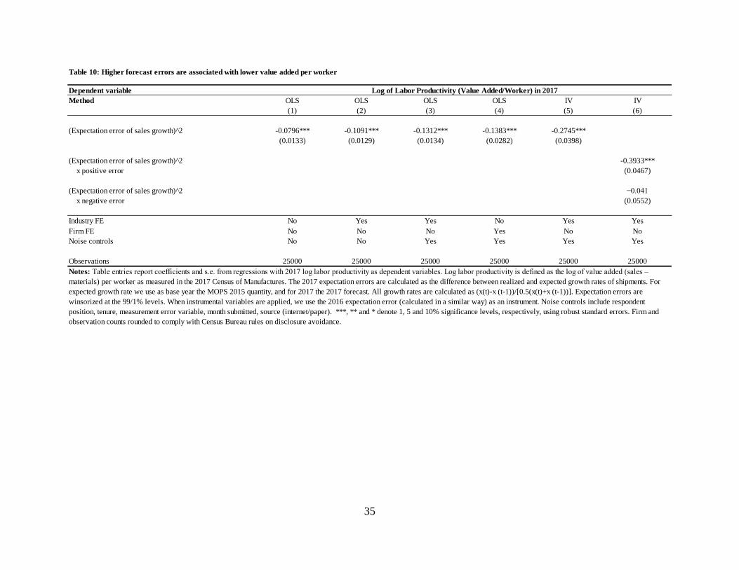
35

Dependent variable

Method OLS OLS OLS OLS IV IV

(1) (2) (3) (4) (5) (6)

(Expectation error of sales growth)^2 -0.0796*** -0.1091*** -0.1312*** -0.1383*** -0.2745***

(0.0133) (0.0129) (0.0134) (0.0282) (0.0398)

(Expectation error of sales growth)^2 -0.3933***

x positive error (0.0467)

(Expectation error of sales growth)^2 −0.041

x negative error (0.0552)

Industry FE No Yes Yes No Yes Yes

Firm FE No No No Yes No No

Noise controls No No Yes Yes Yes Yes

Observations 25000 25000 25000 25000 25000 25000

Notes: Table entries report coefficients and s.e. from regressions with 2017 log labor productivity as dependent variables. Log labor productivity is defined as the log of value added (sales –

materials) per worker as measured in the 2017 Census of Manufactures. The 2017 expectation errors are calculated as the difference between realized and expected growth rates of shipments. For

expected growth rate we use as base year the MOPS 2015 quantity, and for 2017 the 2017 forecast. All growth rates are calculated as (x(t)-x (t-1))/[0.5(x(t)+x (t-1))]. Expectation errors are

winsorized at the 99/1% levels. When instrumental variables are applied, we use the 2016 expectation error (calculated in a similar way) as an instrument. Noise controls include respondent

position, tenure, measurement error variable, month submitted, source (internet/paper). ***, ** and * denote 1, 5 and 10% significance levels, respectively, using robust standard errors. Firm and

observation counts rounded to comply with Census Bureau rules on disclosure avoidance.

Table 10: Higher forecast errors are associated with lower value added per worker

Log of Labor Productivity (Value Added/Worker) in 2017

36

37

38

39

40

41

42

43

44

45

46

47

Appendix

Data cleaning procedure

Forecasting data for 2017 underwent a detailed cleaning process. The cleaning rules included both

flagging categories of responses and, in some cases, editing responses based on those flags. The

editing and imputation rules for these questions are as follows:

1. Create a variable counting the number of missing outcomes (ranges from 0 to 5) and

probabilities (ranges from 0 to 5)

2. Flag any plants that use the same probability distributions across shipments, capital

expenditure, employment, and cost of materials forecasts

3. Flag outcome response patterns that are “1, 2, 3, 4, 5” for the “lowest, low, medium, high, and

highest” scenarios, respectively, when the 2016 point estimate suggests this was simply

numbering the response options

4. Flag response patterns that are the same as the example from the survey instrument

5. Impute missing probabilities with zero

6. Replace outcome values with missing if

a. The reported value of the outcome is negative

b. The probability assigned to the outcome is zero

7. Divide probability by 10 if doing so makes the sum of the five probabilities equal to 100

8. Multiply probabilities by 100 if they sum to one

9. Flag responses with probabilities that sum to 100

10. Flag responses with probabilities that sum to between 90 and 110 (inclusive). These are then

rescaled so that they sum to 100

11. If the response pattern for outcomes is not weakly increasing but adding either one or three

zeroes to one of the low, medium, or high responses would make the outcomes weakly

increasing, then impute the value that would make the outcomes weakly increasing. If changing

more than one response in this manner would make the outcomes weakly increasing, no change

is made.

12. If the response pattern for outcomes is not weakly increasing, but dividing one of the low,

medium, or high responses by 10 or 1000 and truncating the decimal would make the outcomes

weakly increasing, then impute the value that would make the outcomes weakly increasing. If

changing more than one response in this manner would make the outcomes weakly increasing,

no change is made.

13. Impute the low, medium, or high outcomes with the midpoint of the bins above and below if

respondent did not provide a value. If the midpoint cannot be calculated, but two higher (lower)

scenario outcome values are provided, then the value is imputed to be twice the value of the

next higher (lower) scenario less the value of the outcome two positions higher (lower) in the

48

scenario ranking. All probabilities associated with these imputations are zero, so this

imputation does not affect the moments of the forecast distributions but simplifies the

computations of these moments.

14. If the response pattern for outcomes is weakly decreasing, reverse the order of responses and

associated probabilities

15. Create indicator variables for each of the following

a. Outcome distribution is weakly/strictly increasing

b. Probability distribution is symmetric

c. Probability distribution is unimodal

d. Probability distribution is bimodal

e. Probability distribution has an interior mode (i.e. low, medium, or high scenario is most

likely)

f. Probability distribution has a centered mode (i.e. medium scenario is most likely)

g. Outcomes are not all identical

h. Probability distribution does not have 100% assigned to any outcome

i. Probability distribution is uniform

16. Create an indicator variable for “good” responses. The indicator is equal to one if all of the

following hold:

a. Outcome distribution is weakly increasing

b. More than one scenario is reported

c. Probability distribution does not have 100% assigned to any outcome

d. Probabilities sum to between 90 and 110 (inclusive)

e. Responses are not “1, 2, 3, 4, 5” and the respondent’s 2016 estimate suggests this was

not simply numbering the response options

17. Rescale outcome values for shipments, investment, or materials cost by 10κ, κ ϵ {-3, -2, -1, 1,

2, 3} if the ratio of the lowest scenario forecast to the reported value for 2015 is less than

0.15 or greater than 5 and the ratio of the lowest employment forecast to the reported

employment for 2015 is between 0.1 and 10.

18. Trim top and bottom values using the following procedures:

a. If |highest – high| > α*|high – medium| and |highest – high| ≤ β*|high – medium|, for

each of other three questions, then impute highest = high + |high – medium|.

b. If |lowest – low| > α*|low – medium| and |lowest – low| ≤ β*|low – medium|, for each

of other three questions, then impute lowest = low - |low – medium|

19. For all respondents who have data in all ASM survey waves from 2004-2015, responses are

manually reviewed and any typos are corrected.

Editing is less common in responses received electronically because the online form provides built-

in calculation functions and edits that identify potential reporting issues. The former calculated the

49

sum of probabilities provided by the respondent, making it easier for respondents to ensure that

probabilities summed to 100%. Respondents received error messages (that could be ignored) if

response values were not weakly increasing, any cell was left empty, or probabilities did not sum

to 100%. Furthermore, probabilities less than zero or greater than 100 could not be entered in the

online form.

Additional characteristics of survey responses

In section 3, we show that failure to respond to the forecasting questions on the MOPS is

negatively correlated with various observable characteristics of the plant, including structured

management, size, and productivity. One concern, however, is that the failure to provide

responses is a matter of attrition due to the length of the MOPS instrument. Table A4 reports the

number of responses received for specific questions on the 2015 MOPS. We see that the baseline

sample of approximately 35,000 plants respond to the first question on the survey, and roughly

the same number of plants answer the last question on the survey before the uncertainty module.

Approximately 1,500 fewer plants provide their value of shipments for 2015 or a partial year

forecast of the value of shipments for 2016. Fewer plants still provide forecasts for 2017.

Approximately 31,500 respondents provide at least a “medium” forecast of value of shipments

for 2017, while only 30,000 respondents provide a shipments forecast that is considered usable

for our analysis. Our main sample of uncertainty responses, which requires usable forecasts over

all four concepts, is smaller still, at approximately 26,000 plants. However, the lack of a response

does not seem to be mere survey attrition, as many plants who do not provide valid responses for

the uncertainty module return to provide a response to the last question on the survey. The

difference between the number of plants who answer the first question on the survey and the

number who answer the last question is approximately 1,000 plants.

In Table A5, we further examine response quality by respondent title. Of the respondents who

failed to provide a value of shipments for 2015 on the MOPS, the majority were in managerial

positions. This is likely a function of managers being the target respondent for the survey and the

largest share of respondents overall. We see that respondents who are in Human Resources or

administrative positions or do not provide a title are disproportionately less likely to respond

with a value of shipments for 2015. On the other hand, respondents in financial positions are

much more likely to provide this information.

50

Table A1: The Most Common Titles and Categories of MOPS Contacts

Panel A: Categories Share

Manager (except CEO) 53%

Finance (except CFO) 24%

CEO 8%

CFO 5%

HR/admin (non manager) 4%

Missing 6%

Panel B: Titles Share

Plant manager 13%

Financial controller 10%

CEO 5%

CFO 5%

General manager 4%

Other (e.g. vice-president of engineering, COO or production manager) 64%

Table A2: Pairwise correlations

Panel A: Mean expected growth rates ('15-'17)

Shipments Investment Employment Materials

Shipments 1

Investment 0.101 1

Employment 0.39 0.0955 1

Materials 0.488 0.1 0.411 1

Panel B: Standard deviation of expected growth rates ('15-'17)

Shipments Investment Employment Materials

Shipments 1

Investment 0.26 1

Employment 0.472 0.282 1

Materials 0.585 0.295 0.5 1

51

Variable Mean S.D.

Number of

Establishments

Sample with 'Good' forecasts and 2014 & 2015 ASM outcomes 26000

Expected value of 2015-2017 shipments growth rate1

0.0295 0.268

Expected value of 2015-2017 capital expenditure growth rate1

0.117 0.768

Expected value of 2015-2017 employment growth rate1

0.0166 0.198

Expected value of 2015-2017 materials cost growth rate1

0.0417 0.252

Actual 2014-2015 shipments growth rate1

-0.00276 0.287

Actual 2014-2015 capital expenditure growth rate1

0.00429 1.112

Actual 2014-2015 employment growth rate1

0.0292 0.269

Actual 2014-2015 materials cost growth rate1

-0.0281 0.461

Firm-level average standard deviation of 2015-2017 shipments growth rate1

-2.643 0.94

Industry Realized Volatility of Stock Returns -4.033 0.265

Industry Options-Implied Volatility -1.219 0.205

Industry Forecaster Disagreement -3.208 0.607

Industry Dispersion of Stock Returns -4.468 0.274

Sample with at least five years of 2004-2015 ASM/CMF outcomes 17500

Log subjective uncertainty of 2015-2017 shipments growth rate -2.816 0.842

Log subjective uncertainty of 2015-2017 capital expenditure growth rate -1.689 1.2

Log subjective uncertainty of 2015-2017 employment growth rate -3.061 0.852

Log subjective uncertainty of 2015-2017 materials cost growth rate -2.747 0.877

Log volatility of past shipments growth rate -1.657 0.596

Log volatility of past capital expenditure growth rate -0.316 0.224

Log volatility of past employment growth rate -1.976 0.684

Log volatility of past materials cost growth rate -1.327 0.588

Log volatility of parent firm's past shipments growth rate -1.635 0.616

Log volatility of industry's past shipments growth rate -1.425 0.189

Sample of Public Firms 5100

Firm-level average standard deviation of 2015-2017 shipments growth rate1

-2.909 0.748

Firm Realized Volatility of Stock Returns -3.845 0.489

Firm Options-Implied Volatility -1.007 0.408

Sample of Private Firms 21000

Firm-level average standard deviation of 2015-2017 shipments growth rate1

-2.63 0.946

Industry Realized Volatility of Stock Returns -4.028 0.265

Industry Options-Implied Volatility -1.217 0.205

Industry Forecaster Disagreement -3.207 0.609

Industry Dispersion of Stock Returns -4.467 0.273

Sample of Public Firms with at least two I/B/E/S forecasts 3500

Firm-level average standard deviation of 2015-2017 shipments growth rate1

-2.953 0.66

Firm Forecaster Disagreement -2.909 0.91

Sample with 2017 CMF Outcomes 25000

Growth rate of employment, 2015-2017 -0.026 0.359

Growth rate of materials, 2015-2017 0.176 0.652

Growth rate of shipments, 2015-2017 -0.017 0.369

Log(value added/employment), 2017 5.024 0.859

Expected value of 2015-2017 shipments growth rate 0.028 0.193

Standard deviation of 2015-2017 shipments growth rate forecast 0.092 0.316

Squared expectation error for 2015-2017 shipments growth rate1

0.183 0.504

Absolute expectation error for 2015-2017 shipments growth rate1

0.263 0.337

Bias in expectation for 2015-2017 shipments growth rate1

0.046 0.405

1 Winsorized at the 99/1% levels

Table A3: Descriptive statistics

Note: Firm and observation counts rounded to comply with Census Bureau rules on disclosure avoidance.

52

Table A4: Survey flow for the MOPS 2015

Number of Plants

Responded to first question on survey 35000

Responded to last question before uncertainty module 35000

Provided value of shipments for 2015 33500

Provided shipments forecast for 2016 33500

Provided shipments forecast for medium scenario for 2017 31500

"Good" response to 2017 shipments forecast 30000

"Good" response to 2017 shipments, employment, capital

expenditure, and cost of materials forecasts 26000

Answered last question on survey 34000

Notes: Each count provides the number of respondents for specific questions. Firm and

observation counts rounded to comply with Census Bureau rules on disclosure

avoidance.

Table A5: Uncertainty responses distributed over categories of MOPS contacts

Respondent Title Categories No Yes

HR/admin (non manager) 6 4 4

CEO 3 8 8

CFO and other finance 9 30 29

Manager (except CEO) 52 53 53

Missing 30 5 6

Share of Respondents

Provided 2015 Value of Shipments on MOPS?Full Sample

Note: the % of respondents from each main title categories by responding/not-responding to

questions 30 for 2015