NBER WORKING PAPER SERIES

ADDICTION AND CUE-CONDITIONED COGNITIVE PROCESSES

B. Douglas BernheimAntonio Rangel

Working Paper 9329http://www.nber.org/papers/w9329

NATIONAL BUREAU OF ECONOMIC RESEARCH1050 Massachusetts Avenue

Cambridge, MA 02138November 2002

We would like to thank George Akerlof, Gadi Barlevy, Michele Boldrin, Kim Border, Samuel Bowles, ColinCamerer, Luis Corchon, David Cutler, Alan Durell, Victor Fuchs, Ed Glaeser, Jonathan Gruber, JustineHastings, Jim Hines, Matthew Jackson, Chad Jones, Patrick Kehoe, Narayana Kocherlakota, Botond Koszegi,David Laibson, Darius Lakdawalla, Ricky Lam, John Ledyard, George Lowenstein, Ted O’ Donahue, DavidPearce Christopher Phelan, Wolfgang Pesendorfer, Edward Prescott, Matthew Rabin, Paul Romer, PabloRuiz-Verdu, Andrew Samwick, Ilya Segal, Jonathan Skinner, Stephano de la Vigna, Bob Wilson, LeeatYariv, Jeff Zwiebel, seminar participants at U.C. Berkeley, Caltech, Carlos III, Dartmouth, Harvard, HooverInstitution, Instituto the Analysis Economico, LSE, Michigan, NBER, Northwestern, UCSD, Yale,Wisconsin-Madison, SITE, Federal Reserve Bank of Minneapolis, and the McArthur Preferences Networkfor useful comments and discussions, and Luis Rayo for outstanding research assistance. Antonio Rangelgratefully acknowledges financial support from the NSF (SES-0134618), and thanks the Hoover Institutionfor its financial support and stimulating research environment. This paper was prepared in part whileBernhiem was a Fellow at the Center for Advanced Study in the Behavioral Sciences (CASBS), where he wassupported in part by funds from the William and Flora Hewlett Foundation (Grant #2000-5633). The viewsexpressed herein are those of the author and not necessarily those of the National Bureau of EconomicResearch.

© 2002 by B. Douglas Bernheim and Antonio Rangel. All rights reserved. Short sections of text, not toexceed two paragraphs, may be quoted without explicit permission provided that full credit, including ©notice, is given to the source.

Addiction and Cue-Conditioned Cognitive ProcessesB. Douglas BernheimAntonio RangelNBER Working Paper No. 9329November 2002JEL No.D0, D1, D6, D9, H0, H2, H5, I0, I1, K1, K4

ABSTRACT

We propose an economic theory of addiction based on the premise that cognitive mechanisms

such as attention affect behavior independently of preferences. We argue that the theory is consistent with

foundational evidence (e.g. from neuroscience and psychology) concerning the nature of decision-making

and addiction. The model is analytically tractable, and it accounts for a broad range of stylized facts

concerning addiction. It also generates a plausible qualitative mapping from the characteristics of

substances into consumption patterns, thereby providing a basis for empirical tests. Finally, the theory

provides a clear standard for evaluating social welfare, and it has a number of striking policy implications.

B. Douglas Bernheim Antonio RangelDepartment of Economics Department of EconomicsStanford University Stanford UniversityStanford, CA 94305-6072 Stanford, CA 94305-6072and NBER and NBERbernheim@stanford.edu rangel@leland.stanford.edu

1

1 Introduction

Each year, millions of U.S. consumers spend hundreds of billions of dollars on addic-

tive substances.1 Estimates for 1999 place total expenditures on tobacco products,

alcoholic beverages, cocaine, heroin, marijuana, and methamphetamines at more than

$150 billion. During a single month in 1999, more than 57 million individuals smoked

at least one cigarette, more than 41 million engaged in binge drinking (involving five or

more drinks on one occasion), and roughly 12 million used marijuana. In 1998, slightly

more than 5 million Americans qualified as “hard-core” chronic drug users. Roughly

4.6 million persons in the workforce met the criterion for a diagnosis of drug dependence

and 24.5 million had a history of clinical alcohol dependence. In 1998, additional social

costs resulting from health care expenditures, loss of life, impaired productivity, motor

vehicle accidents, crime, law enforcement, and welfare totalled $185 billion for alcohol

and $143 billion for other addictive substances. Smoking killed roughly 418,000 people

in 1990, alcohol accounted for 107,400 deaths in 1992, and drug use resulted in 19,277

deaths during 1998. Alcohol abuse contributed to 25 to 30 percent of violent crimes.

In 1999, more than 625,000 individuals were incarcerated for drug-related offenses.

Public policies regarding addictive substances run the gamut from laissez faire to

taxation, subsidization (e.g. of rehabilitation programs), regulated dispensation, crim-

inalization, product liability, and public health campaigns. Each alternative policy

approach has passionate advocates and detractors. Economic analysis can potentially

inform this debate, but it requires the analyst to adopt a theory of addiction.

The ideal economic theory of addiction would satisfy four criteria. First, it would

be consistent with foundational evidence (e.g. from neuroscience and psychology) con-

cerning the nature of decision-making and addiction. Second, it would account for the

salient aspects of addictive behavior. Third, it would lend itself to tractable mathe-

matical modeling. Fourth, it would provide a clear standard for policy evaluation (i.e.

the measurement of social welfare).

A number of authors (such as Becker and Murphy [1988], Laibson [2001], Hung

[2000], and Orphanides and Zervos [1995]) have proposed theories of addiction based

on standard economic models of decision making. Others (such as Gul and Pesendorfer

[2001b], Laibson [2001], and Gruber and Koszegi [2001]) have explored various “behav-

ioral” alternatives. Unfortunately, as we discuss in we section 2, each of these theories

falls short of the ideal. Among other shortcomings, each fails to explain important

aspects of addictive behavior.

1The statistics in this paragraph were obtained from the following sources: Office of National Drug

Control Policy [2001a,b], U.S. Census Bureau [2001], Gerstein et. al. [1999], National Institute on

Drug Abuse [1998], National Institute on Alcohol Abuse and Alcoholism [2001], and Center for Disease

Control [1993]. There is, of course, disagreement as to many of the reported figures.

2

The purpose of this paper is develop an alternative theory of addiction that satisfies

the four criteria articulated above. As our starting point, we depart fundamentally

from standard economic theory by accepting the validity of the hypothesis that cogni-

tive mechanisms such as attention, which determine how an individual thinks about a

decision, affect behavior entirely apart from preferences. For example, an individual

may fail to choose an alternative simply because he does not consider it, or because he

fails to consider particular consequences. When this occurs, the individual may choose

something other than the alternative that he would most prefer if he considered all op-

tions and consequences. Since this mistake results from an improper characterization

of the decision problem, we refer to the phenomenon as characterization failure.

Our theory proceeds from the premise that environmental cues affect the way the

brain characterizes decision problems. In particular, with experience, the brain devel-

ops cognitive shortcuts involving functions such as attention. These shortcuts appear

to be mediated by, or at least associated with internal visceral states. For example,

when someone notices the familiar smells of a barbecue, he experiences visceral sen-

sations of hunger, and his thoughts turn to the acquisition and consumption of food.

The use of a cognitive shortcut does not necessarily lead to characterization failure;

on the contrary, an efficient shortcut could economize on the costs of decision making

by focusing attention on the most promising alternatives and pertinent consequences.

Nevertheless, in the context of addictive substances, the evidence suggests that cog-

nitive shortcuts focus attention on inappropriate actions and consequences given the

individual’s objectives and preferences. Thus, environmental cues associated with past

usage influence current use through cognition (e.g. which alternatives and consequences

capture the brain’s attention) as well as through preferences.

We provide a parsimonious representation of this phenomenon in an otherwise stan-

dard model of rational addiction. Specifically, we allow for the possibility that the

individual may enter a “hot” cognitive mode in which he always chooses to consume

the substance irrespective of underlying preferences (implicitly because inappropriate

cognitive shortcuts focus attention on usage and the associated “high”), and we assume

that the likelihood of entering this state is related to past choices (implicitly because,

through conditioning, previous usage increases the probability of encountering environ-

mental cues which trigger the hot cognitive mode). The individual may also operate

in a “cold” cognitive mode, wherein he considers all alternatives and contemplates all

consequences, including the effects of current choices on the likelihood of entering the

hot cognitive mode in the future.2

2Our analysis is most closely related to work by Loewenstein [1996,1999], who considers simple

models in which an individual can operate in either a hot or cold decision-making mode. Lowenstein’s

approach differs from ours in at least one important respect: he assumes that behavior in the hot mode

reflects the application of a “false” utility function, rather than a particular (and potentially flawed)

3

As a matter of formal mathematics, our model involves a minimalistic departure

from the standard framework. Behavior corresponds to the solution of a dynamic

programming problem with stochastic state-dependent mistakes. Our approach there-

fore harmonizes economic theory with foundational evidence on decision making and

addiction without sacrificing analytic tractability.

The model has several attractive features. It explains a broad range of important

stylized facts associated with addiction. It generates a plausible qualitative mapping

from the characteristics of substances into consumption patterns, thereby providing

the basis for empirical tests. It gives rise to a clear welfare criterion, and it has some

surprising public policy implications. For example, in some circumstances it is optimal

to subsidize the use of addictive substances even though consumption is excessive. Yet

under the same circumstances, criminalization may be superior to taxation.

The remainder of the paper is organized as follows. Section 2 describes patterns

of addictive behavior. It also briefly summarizes and evaluates existing theories of

addiction. Section 3 discusses foundational evidence concerning the nature of decision-

making and addiction. Section 4 presents our formal model. Section 5 explores the

model’s positive implications, including its ability to generate observed consumption

patterns and to explain the main stylized facts concerning addiction. Section 6 exam-

ines the welfare implications of various public policies. Section 7 concludes. Proofs

of propositions appear in an appendix.

2 Addictive Behavior

2.1 Patterns of addictive behavior

The consumption of addictive substances has received substantial attention in neu-

roscience, psychology, epidemiology, sociology, and economics.3 From this extensive

body of research, we have distilled eight stylized facts which, we argue, should serve as

a litmus test for evaluating the validity of any economic theory of addiction.

First, short-term abstention is common even for the most addictive substances, but

long-term recidivism rates are high (see Goldstein [2001], Hser, Anglin, and Powers

[1993], Harris [1993], and O’Brien [1997]). In many instances, addicts attempt to “kick

the habit,” but are ultimately unsuccessful. For example, during 2000, 70 percent of

current smokers expressed a desire to quit completely and 41 percent stopped smoking

mode of cognition. See also Loewenstein and Lerner [2001] for an excellent review of the evidence

concerning the effects of emotions and visceral states on decision-making.3Gardner and David [1999] provide the following list of addictive substances: (1) alcohol, (2) bar-

biturates, (3) amphetamines, (4) cocaine, (5) caffeine and related methylxanthine stimulants, (6)

cannabis, (7) hallucinogenics, (8) nicotine, (9) opioids, (10) dissociative anasthetics, and (11) volatile

solvents.

4

for at least one day in an attempt to quit, but only 4.7 percent successfully abstained

for more than three months.4

Second, consumption and recidivism are associated with cue-conditioned cravings.

Recidivism rates are especially high when addicts are exposed to cues related to

their past drug consumption (Goldstein [2001], Goldstein and Kalant [1990], O’Brien

[1976,1997], Robins [1974], Robins et. al. [1974], and Hser et. al.). Long-term usage

is considerably lower among those who experience significant changes of environment.5

For this reason, drug treatment programs advise recovering addicts to move to new

locations, or at least to avoid the places where previous consumption took place. A

recovering addict is also significantly more likely to “fall off the wagon” if he receives a

small taste of his drug-of-choice (Goldstein [2001]). This phenomenon, known as “prim-

ing,” suggests that even minimal exposure to the substance serves as a powerful cue

that activates cravings.

Third, addicts continue to use drugs compulsively even though with sufficiently

sustained use they develop tolerance with respect to the hedonic effects of the sub-

stance (i.e., the quality and intensity of the high often diminishes despite increases in

dosage). The development of hedonic tolerance is a complex process.6 For some drugs,

such as cocaine, users experience a phenomenon called sensitization, in which the he-

donic effects of the drug are enhanced in the short term, for example during binges.

Nevertheless, there is some agreement that a large fraction of substances and users

develop hedonic tolerance with sustained use. In a recent review of the neurobiology

of addiction, Hyman and Malenka [2001,p. 695] observe:

“The desire to elevate or otherwise alter mood often motivates initial

drug use. However, the pleasure (or relief of dysphoric moods) produced

by drugs often habituates; for drugs such as alcohol and nicotine, pleasure

can be markedly reduced over time by medical complications. Addictive

individuals sometimes describe their continuing drug use as an attempt to

re-experience remembered ‘highs’ often without success.”

Similarly, Goldstein [2001, p. 86] states that “with most addictive drugs, repeated

4Notably, more educated individuals were far more likely to quit successfully, even though education

bore little relation either to the desire to quit or to the frequency with which smokers attempted to

quit (Trosclair et. al. [2002]).5Robins [1974] and Robins et.al. [1974] found that Vietnam veterans who were addicted to heroin

and/or opium at the end of the war experienced much lower relapse rates than other young male addicts

during the same period. A plausible explanation is that veterans encountered fewer environmental

triggers (familiar circumstances associated with drug use) upon returning to the U.S.6The term tolerance is used to describe a wide range of physical adaptations that take place in

response to the addictive substances. For example, with repeated usage, the body (in particular the

liver) develops an increased capacity to destroy the drug. This leads to a phenomenon called metabolic

tolerance (see Goldstein [2001]).

5

administration over a long time ... leads to a loss of effect, so that more and more

is needed to produce the same high as before.” A user-oriented website concurs:7

“Tolerance builds up rapidly after a few doses and disappears rapidly after a couple of

days of abstinence. Heavy users need as much as eight times higher doses to achieve

the same psychoactive effects as regular users using smaller amounts. They still get

stoned but not as powerfully.”

Fourth, addicts often describe themselves as powerless to regulate their consumption

of the substance. They perceive some of their past choices as mistakes, in the sense that

they think they would have been better off in the past as well as the present had they

acted differently, even when no learning has occurred. They sometimes characterize

current choices as mistakes even in the act of consumption.8 They also recognize

that they are likely to make similar mistakes in the future. It is instructive that the

twelve-step program of Alcoholic Anonymous begins as follows: “We admitted we were

powerless over alcohol - that our lives had become unmanageable.”9

Fifth, users respond to standard economic incentives such as prices and information

about the effects of addictive substances.10 For example, an aggressive U.S. public

health campaign is widely credited with reductions in rates of cigarette smoking. There

is also evidence that users engage in sophisticated forward-looking deliberation, reduc-

ing current consumption in response to future price increases (Gruber and Koszegi

[2001]).

Sixth, addicts attempt to control use through various pre-commitments, such as

checking into rehabilitation centers and consuming medications that either generate

unpleasant side effects or reduce pleasurable sensations if the substance is subsequently

consumed. Disulfiram interferes with the liver’s ability to metabolize alcohol; as a

result, ingestion of alcohol produces a highly unpleasant physical reaction for a period

of time. Methadone, an agonist, activates the same opioid receptors as heroin, and

thus produces a mild high, but has a slow-onset and a long-lasting effect. It thereby

reduces the high produced by heroin. Naltrexone, an antagonist, blocks specific brain

receptors, and thereby diminishes the high produced by opioids. All of these treatments

reduce the frequency of relapse.11

Seventh, use is sensitive to the deployment of attention. Exogenous attention

shocks can temporarily discourage use without providing new information. A recover-

7See htpp://www.thegooddrugsguide.com/cannabis/addiction.htm.8Goldstein [2001,p.249] describes this phenomenon as follows: the addict had been “suddenly

overwhelmed by an irresistible craving, and he had rushed out of his house to find some heroin.

... it was as though he were driven by some external force he was powerless to resist, even though he

knew while it was happening that it was a disastrous course of action for him” (italics added).9See http://www.alcoholics-anonymous.org/english/E FactFile/M-24 d6.html.

10See Chaloupka and Warner [2001] and MacCoun and Reuter [2001] for a review of the evidence.11See O’Brien [1997] and Goldstein [2001].

6

ing addict is, for example, less likely to use (at least temporarily) if, while experiencing

a strong craving, he is reminded of undesirable consequences with which he is already

familiar.12 Consequently, recovering addicts exhibit a demand for attention manage-

ment therapies. Even addicts who have stayed clean for years attend support group

meetings, such as Alcoholics Anonymous, which provide no new information.13

Eighth, patterns of usage vary dramatically across addictive substances and, for

any given substance, across methods of administration and users. Caffeine is con-

sumed on a regular basis and users rarely seek clinical intervention to control use,

while cocaine users experience binging cycles and sometimes seek institutional reha-

bilitation. Cocaine and crack, though chemically identical, give rise to different con-

sumption patterns.14 Although a sizable fraction of the population either experiments

with drugs or uses for recreation, most do not become clinically addicted.15

2.2 Existing theories

Existing economic theories of addiction include (1) variations on the standard model

of rational economic decision making (Becker and Murphy [1988]), including general-

izations that allow for random shocks and state-contingent utility (Laibson [2001] and

Hung [2000]), (2) models of “temptation” wherein well-being depends not only upon

the chosen action but also on actions not chosen (Gul and Psendorfer [2001a,2001b]

and Laibson [2001]), (3) models with present-biased preferences with either naive or so-

phisticated expectations (O’Donoghue and Rabin [1999,2000] and Gruber and Koszegi

[2001]), and (4) models with “projection bias,” wherein agents mistakenly assume

that future preferences will resemble current preferences (Loewenstein [1996,1999], and

Loewenstein, O’Donoghue, and Rabin [2001]). Each of these theories contributes to

an understanding of decision-making in general and addiction in particular. Although

a comprehensive discussion of the various behavioral alternatives is beyond the scope

of the current paper, it is important to highlight some limitations of these approaches.

For a more complete discussion, see Bernheim and Rangel [2002].

12There are, for example, references to the role of attention shocks in Massing [2000], who provides

detailed descriptions of addicts’ experiences.13Goldstein [2001] reports that there is a shared impression among the professional community

that 12-step programs such as AA (p. 149) “are effective for many (if not most) alcohol addicts.”

However, given the nature of these programs, objective performance tests are not available. The AA

treatment philosophy is based on “keeping it simple by putting the focus on not drinking, on attending

meetings, and on reaching out to other alcoholics.” Goldstein also notes that, according to AA, there

are recovering alcoholics, but not ex-alcoholics; hence the dictum “once an addict, always an addict.”14Crack is prepared from cocaine by mixing it with baking soda and water, and then boiling it. This

has two important consequences. First, crack can be smoked, which allows the brain to absorb the

substance more efficiently, and leads to a quicker and more intense high. Second, crack is significantly

cheaper, which leads to a pattern of more frequent administration.15See Goldstein and Kalant [1990], Gazzaniga [1990,1994], and Koob and Moal [1997].

7

With respect to the first stylized fact, all of the preceding theories can, under

appropriate assumptions, account for cycles of use and abstention, as well as for quitting

by some users. If, however, one interprets an intention to quit “completely” as referring

to all future contingencies, then recidivism among intended quitters involves a failure

to follow through on a contingent plan.16 Such failures can occur with present-biased

preferences if expectations are naive, or with projection bias, but they are inconsistent

with the other possibilities mentioned above.

All of the existing theories are at odds with the third stylized fact, since they assume

that the addictive substances are distinguished by intertemporal complementarities

in consumption: the marginal utility of using the substance is assumed to increase

with previous consumption. In fact, without intertemporal complementarities nothing

would distinguish addictive and non-addictive substances; the very same self-control

problem would influence the consumption of all immediately pleasurable activities,

from injecting heroin to drinking water.

With respect to the fourth stylized fact, none of the existing theories can account

for the observation that addicts sometimes describe their current choices as mistakes.

In each instance, the decision maker maximizes a utility function that describes his

well-being at the time of choice. The anticipation of future mistakes is inconsistent

with the standard model, temptation preferences, hyperbolic discounting with naive

expectations, and projection bias. In each of these cases individuals believe that their

future behavior will be optimal when evaluated by current preferences.17 With present-

biased preferences and sophisticated expectations, the individual anticipates that future

choices may be contrary to his current desires; however, he recognizes that those choices

will be optimal for his in the future, and hence will not be mistakes when he makes

them. Finally, all of these models are unable to account for the perception that past

choices were mistakes. In every case, an individual might regret a past choice in the

sense that he would be better off today had he acted differently, but he never believes

that an alternative choice would have made him better off in the past as well as the

present.

With respect to the sixth stylized fact, the standard framework is capable of ex-

plaining voluntary admission to rehabilitation clinics and related behaviors provided

that these activities reduce the likelihood of experiencing cravings. But this is contrary

to the experience of many addicts who check into rehabilitation centers not because

they expect to avoid cravings, but rather precisely because they anticipate cravings and

16According to Hyman and Malenka [2001,p.697], there is agreement that “cue-initiated relapses can

occur in individuals who have strongly resolved never to use drugs again, often without the addicted

person having insight into what is happening to them” (italics added).17Although this belief is false in the last two cases, individuals nonetheless fail to anticipate future

mistakes.

8

wish to control their reactions. Furthermore, even in instances where entering a reha-

bilitation center does reduce the likelihood of cravings (e.g. by removing environmental

cues), the standard framework implies counterfactually that the addict would find the

center’s program more attractive if it made the substance available upon request (in

case of cravings). Likewise, the standard framework is hard-pressed to explain the

voluntary use of substances such as disulfiram, which simply reduce the utility derived

from future usage. More generally, within the standard framework, the decision-maker

would avoid precommitments (decisions that eliminate future options). Similar com-

ments apply for models with projection bias, and with present-biased preferences and

naive expectations. Models with temptation preferences can explain precommitments,

but only if the elimination of the tempting alternative suppresses cravings. For the

reasons described above, this explanation is problematic. Among the existing alter-

natives, only present-biased preferences with sophisticated expectations can account

adequately for the fifth stylized fact.

All of the theories mentioned above also struggle to account for the seventh stylized

fact. Since behavior is, in each instance, a direct manifestation of preferences at each

moment in time, attention shocks cannot affect behavior.18

The second, fifth, and eighth stylized facts pose fewer problems for existing theories.

Even though the literature contains many models of addiction that do not specifically

encompass cue-conditioned cravings, an appropriately articulated version of each ex-

isting theory can nevertheless account for the second stylized fact (see, for example,

Laibson’s [2001] extension of Becker and Murphy’s [1988] model). With intertempo-

ral complementarities, these theories are also consistent with evidence indicating that

usage is sensitive to both current and future economic incentives (the fifth stylized

fact). While there has been no systematic attempt to account for the heterogeneity

of consumption patterns across addictive substances, methods of administration, and

users (the eighth stylized fact), each theory provides many dimensions of flexibility.

Additional reservations concerning existing theories of addiction include the fol-

lowing. First, some of the existing theories lack explicit neuro foundations. They

are not intended to depict actual decision-making processes; rather, they are strictly

“as if” representations of behavior. Second, some of the alternatives sacrifice math-

ematical tractability (relative to the standard model). Models with present-biased

preferences introduce strategic considerations, and require one to depict behavior as

the equilibrium of a game played between the decision-maker and his future incarna-

tions. These equilibria can be extremely complex and challenging to characterize.

18This is not to say that the concept of attention is in itself problemmatic. As discussed in section 3,

even the standard framework can accomodate the notion that attention and preferences shift together

in response to environmental cues. It is more challenging, however, to account for the observation

that individuals learn to manage behavior by managing attention.

9

It can also be difficult to analyze models of temptation when preferences are defined

over sets rather than over choices.19 Third, with either present-biased preferences

or temptation preferences, welfare is often ambiguous and a matter of the perspective

chosen for evaluation.

3 Foundations

Our objective in this paper is to explain addictive behavior based on general principles

concerning decision making, rather than as an idiosyncratic special case. The general

principles that we invoke allow for the possibility that the cognitive portions of the

brain’s decision-making algorithms perform poorly in identifiable circumstances. We

argue that addiction is a particularly severe instance of this phenomenon. In this

section, we discuss the available evidence concerning these foundational hypotheses.

3.1 Cue-Conditioned Characterization Failure

Decision making involves (at least) three types of processes: characterization, evalu-

ation, and hedonic experience. Characterization entails the deployment of cognitive

mechanisms such as attention, memory, and forecasting to identify the state of the

world, the set of possible actions, and the present and future consequences of each

action. Evaluation refers to the process by which the brain assesses the desirability of

each action under consideration in light of its projected consequences and the state of

the world. Finally, a hedonic experience, consisting of both pleasant and unpleasant

sensations, results from the state of the world and the consequences of choices.

Under appropriate assumptions concerning these three processes, one obtains the

standard model of economic decision-making. For example, one could assume that

the brain completely and correctly extrapolates the consequences of all possible alter-

natives during the characterization stage, and selects among these alternatives using a

criterion that corresponds to maximization of discounted expected hedonic experience

during the evaluation stage. In this paper we investigate the implications of more

realistic assumptions concerning the nature of characterization. We note that there

may also be valid reasons to depart from standard assumptions concerning evaluation

and experience, but we do not pursue these possibilities here (see Bernheim and Rangel

[2002] for a discussion of evidence regarding the other two processes).

Since the brain is a finite computational mechanism, it cannot consider every pos-

sible option and forecast every potential consequence. Characterization shortcuts are

thus unavoidable. Given the current state of knowledge, it is not yet possible to describe

19Gul and Pesendorfer [2001a] demonstrate that one can depict choice with temptation as the

solution to a fairly standard dynamic program under appropriately strong assumptions.

10

cognitive decision-making algorithms with precision. Nevertheless, recent research find-

ings in psychology and neuroscience provide foundations for three general principles.

First, emotional and visceral states (e.g. anger or cravings) affect cognitive activities,

including attention, that play a central role in characterization. Second, certain en-

vironmental cues systematically trigger particular visceral states and the associated

cognitive modes. Third, these triggers are established through a form of learning

called cue-conditioning: with experience the brain learns to associate particular cues

with the visceral states that guide cognition to hedonically salient states, options and

consequences.

We illustrate these three principles through a simple example. When an individual

is hungry (a visceral state), his attention focuses on tasks associated with obtaining

food. Specific environmental cues, such as the smell of a barbecue, can trigger sen-

sations of hunger. Far from being hard-wired, this response is cue-conditioned: the

aroma triggers hunger because the individual has had the pleasurable experience of

consuming food at previous barbecues.

The use of cue-conditioned cognitive shortcuts does not by itself overturn the stan-

dard model. If, for example, visceral and emotional signals guide attention to ap-

propriate subsets of alternatives and consequences, the brain may select an optimal

or nearly optimal alternative even though it characterizes only a small portion of the

decision problem. In fact, the use of such shortcuts could be an effective evolutionary

adaptation. The problem, as emphasized by evolutionary psychologists (see Barkow,

Cosmides, and Tooby [1995]), is that brain processes evolved to promote fitness in the

hunter-gatherer world, not in the modern world. Thus, for example, panic-triggered

flight responses that helped humans escape from predators as hunter-gatherers may be

counterproductive when judged by the individual’s own objectives and preferences in

many modern situations.

Accordingly, we depart from the standard model by assuming that, in some cir-

cumstances, environmental cues can induce visceral states that divert attention from

the most preferred alternatives and/or hedonically salient consequences. When this

happens, the ability of the brain to choose the most preferred option is impaired. We

refer to this phenomenon as cue-conditioned characterization failure.

If an individual repeatedly experiences characterization failure upon encountering

particular environmental conditions, he may learn to associate those conditions with

poor decision-making. This type of self-understanding may lead to a range of inter-

esting and economically important behavioral patterns. For example, individuals may

avoid situations in which they are exposed to certain cues (cue avoidance), attempt

to preclude alternatives that they tend to choose when experiencing characterization

failure (precommitment), desensitize themselves to problematic cues, or develop self-

11

management techniques to counteract the effects of strong visceral states (such as

counting to ten before acting).

Research in several disciplines provides foundational evidence for various aspects of

the hypotheses described above. First, visceral states appear to influence the outcome

of decision-making even when they are arguably uncorrelated with pertinent aspects of

preferences. Shoppers tend to purchase more food at the grocery store when they are

hungry, even though they know that the state of hunger is temporary (see Abratt and

Goodey [1990]). A variety of tactics used in the contexts of interrogations and legal

depositions are intended to elicit responses with long-lasting implications by induc-

ing transitory emotional reactions (Loewenstein [1996]). Likewise, salespeople often

attempt to influence consumers’ choices by manipulating visceral desires through en-

vironmental cues, even when the good in question is durable while the visceral state is

not.

Second, a series of experiments by Mischel and coauthors suggest that self-control

is sensitive to the deployment of attention and to the activation or non-activation of

particular thoughts.20 A subject (typically a child) is placed in a room and is offered

a choice between an inferior prize and a superior one (one or two pieces of candy).

Subjects can obtain the inferior prize at any time by calling the experimenter, but

must wait until the experimenter returns to obtain the superior prize. In practice, the

child’s ability to wait depends crucially on whether the inferior prize is visible. Merely

covering the object significantly enhances patience.

More generally, in Mischel’s experiments, the deployment of attention emerges as a

key determinant of self-control. Any stimulus that focuses attention on the “tempting”

features of the inferior prize increases the likelihood that the child will select it. Chil-

dren are significantly more likely to wait if they are advised to distract themselves by

thinking about something else, or if they are provided with a toy, even when children

in a control group show no interest in the toy. Advising children not to think about

the prize is counterproductive, since this induces them to repeatedly check whether or

not they are thinking about it, thereby inadvertently activating thoughts about the

prize.21 During the course of development, children acquire self-understanding, and

begin to consciously regulate thought-generating environmental cues (“metacognitive

awareness”).22 When asked whether they would prefer to have the prize exposed or

covered, children under four exhibit no preference and are unable to justify their choice.

In contrast, those over five prefer to wait with the prize hidden, and offer explanations

that suggest some understanding of the principle that exposure to the prize influences

20See Mischel [1974], Mischel and Moore [1973], Mischel, Shoda, and Rodriguez [1992], and Metcalfe

and Mischel [1999].21This variation of the experiments is closely related to the work of Wegner [1994].22See Metcalfe and Mischel [1999].

12

attention. These findings are consistent with the hypothesis that seeing or think-

ing about the prize triggers strong visceral states (cravings) that restrict the child’s

subsequent thoughts to a limited range of activities and outcomes.23

In some settings, there is also direct evidence that visceral states influence behavior

by restricting attention to limited sets of alternatives and consequences. In particular,

fear focuses attention on the possibility of environmental threats (Janis [1967]) and on

a limited number of “fight-or-flight” responses (Panksepp [1988], ch. 11).

Third, research in neuroscience has identified some of the mechanisms through

which visceral states influence choice by altering cognition. LeDoux’s work on fear

is a leading example.24 Information about the environment reaches the amygdala (a

primitive brain structure that helps to initiate responses to sensory stimuli) via two

principal routes: a short “direct” route, and a long cortical route. Along the first

route, information passes directly from the sensory thalamus to the amygdala without

intermediate processing by the neocortex. Along the second route, information is sent

from the sensory thalamus to various neocortical structures, where it is processed be-

fore proceeding to the amygdala. The short route is more primitive (in an evolutionary

sense) and permits the organism to initiate rapid responses in critical survival situa-

tions. Though slower, use of the long route permits more deliberate responses. The

existence of the short route implies that, in some circumstances, human behavior can

result with little (if any) cognitive deliberation.25

Finally, research in neuroscience also suggests that individuals cannot make sound

decisions unless visceral states guide cognition. This principle finds support in a series

of influential neurological studies by Antonio Damasio and various coauthors concerning

the decision-making abilities of patients with damage to the ventromedial sector of the

prefrontal cortex.26 Injuries of this variety lead to abnormal (often muted) emotional

responses, even though a standard battery of tests reveals no cognitive impairments.

Although their “logical” reasoning facilities are intact, these individuals nevertheless

exhibit an impaired capacity for sound decision making. Based on these findings,

Damasio has formulated the “somatic marker hypothesis,” which holds that, in normal

individuals, the brain uses visceral states to simplify complex decision problems. In

Damasio’s theory, the ventromedial frontal cortex contains dispositional information

23Metcalfe and Mischel [1999] reach similar conclusions.24See LeDoux [1992,1993,1998] and also Davis [1992a,1992b].25Consider the following example (LeDoux, [1998]). While hiking through a park, an individual

glimpses a long stick, resembling a snake, lying on the ground. This information first reaches his

amygdala through the short route. The amygdala automatically initiates defensive responses, includ-

ing autonomic changes such as increased blood circulation, endocrine changes such as the release of

adrenaline, and neocortical changes such as heightened alertness. Before consciously thinking about

alternatives, the hiker stops short or leaps to safety.26See Damasio [1994], Behara et al. [1996,1997], and Bechara et. al. [1994].

13

which is accumulated through experience. In any given visceral state, pre-conscious

processing uses this information to identify appropriately “marked” alternatives, which

then receive conscious consideration.

3.2 Addictive Substances and Cue-conditioned Characteriza-

tion Failure

For several decades neurobiologists have recognized that a variety of addictive sub-

stances, from alcohol to cocaine, have a powerful impact on the brain’s mesolimbic

dopamine system (MDS) (see, for example, Hyman and Malenka [2001], Nestler [2001],

and Wickelgreen [1997] for recent reviews).27 The MDS, in turn, plays a central role

in the regulation of basic behaviors. For example, experiments have shown that rats

who are given drugs that block dopamine receptors, thereby impeding the appropriate

operation of the MDS, eventually stop feeding (Berridge [1999]).

Experiments have also shown that direct stimulation of the MDS is a powerful way

to induce experimental subjects to perform a behavior. For example, in a series of

classic experiments, Olds and Milner [1954] demonstrated that rats learn to return

to locations where they have received direct electrical stimulation to the MDS. When

provided with opportunities to self-administer by pressing a lever, the rats rapidly

became addicted, giving themselves approximately 5,000-10,000 “hits” during each

one hour daily session, ignoring food, water, and opportunities to mate. Addicted rats

were willing to endure painful electric shocks to reach the lever.28 Similarly, when rats

are allowed to self-administer cocaine, they ignore hunger, reproductive urges, and all

other drives, consuming the substance until they die (Pickens and Harris [1968] and

Gardner and David [1999]).

Based on these findings, researchers proposed a variety of theories that linked the

consumption of addictive substances to the their ability to generate enormous hedonic

rewards (the “high”) by stimulating the MDS. This view parallels existing economic

theories in which users consume addictive substances to maximize pleasure.

Neurobiological support for this “pleasure principle” theory of addiction has eroded

over the course of the last decade with the accumulation of new evidence indicating

that MDS activity does not exclusively, and perhaps not even primarily, relate to the

27Of the addictive substances listed in a previous footnote, only hallucinogenics (or psychedelics)

do not seem to produce intense stimulation of the MDS. Instead, they act on a “subtype of serotonin

receptor which is widely distributed in areas of the brain that process sensory inputs” (Goldstein

[2001, p.231]). There is some disagreement as to whether hallucinogens are properly classified as

addictive substances (see Goldstein [2001, ch. 14]). Notably, laboratory animals and humans learn

to self-administer the same set of substances, with the possible exception of hallucinogenics (Gardner

and David [1999, p.97-98]).28See Gardner and David [1999] for a summary of these experiments.

14

generation of pleasure.29 This evidence includes the following findings. First, unpleas-

ant and novel stimuli that are hedonically neutral also trigger a release of dopamine

(Becerra et. al. [2001] and Schultz [1998, 2000]). Second, dopamine surges in anticipa-

tion to rewards, or cues associated with rewards, not during or after their consumption.

Furthermore, dopamine cells respond to rewards only when they occur unexpectedly.

This suggests that the MDS acts more as a learning mechanism than as a hedonic

meter (see Schultz, Dayan, and Montague [1997], and Schultz [1998, 2000]). Third,

using advanced imaging technology, Breiter et. al. [1997] have scanned addicts’ brains

during complete usage episodes, and found that the dopamine system remains active

long after the “high” has passed. Fourth, rats have normal hedonic reactions to sweet

and bitter tastes, and can learn about new hedonic stimuli, even when their ability

to transmit dopamine has been impaired through the administration of a neurotoxin

(Berridge and Robinson [1998]).

The accumulating evidence has lead neurobiologists to a new consensus view of

addiction. In this view, addictive substances directly affect brain processes, such as

memory and attention, that are central to deliberative decision-making. Moreoever,

these effects are poorly correlated with hedonic pleasure (i.e., preferences). According

to Hyman and Malenka’s [2001, p. 703] review of the pertinent literature, “recent ev-

idence ... (suggests) that the central behavioral features of addiction result from the

ability of drugs to usurp normal mechanisms of memory in crucial survival circuits.”30

This may help to explain the observation that addicts’ thoughts tend to focus almost

exclusively on consumption of substances during binges and while experiencing crav-

ings (Gawin [1991]).31 Notably, the literature draws a distinction between liking a

substance, which results from the experience of hedonic pleasure, and wanting a sub-

stance, which refers to aspects of decision processes that incline an addict towards

usage. It also emphasizes that wanting and liking are not always aligned. Robin-

son and Berridge [2000,p. 91] conclude that “the brain systems that are sensitized do

not mediate the pleasurable or euphoric effects of drugs (drug ‘liking’), but instead

29Wickelgreen [1997, p. 35] quotes Roy Wise, one of the individuals who originally proposed the

pleasure principle theory of addiction, as follows: “I no longer believe that the amount of pleasure felt

is proportional to the amount of dopamine floating around in the brain.”30Vorel et. al. [2001] have shown that the stimulation of memory centers can trigger strong cravings

and recidivism among rats that have previously self-administered cocaine (Vorel and Gardner [2001]

and Holden [2001a,b] provide non-technical discussions). Ungless et. al. [2001] have shown that

similar cellular mechanisms may be at work in memory and addiction (see Helmuth [2001] for a

non-technical discussion).31Tiffany [1990, p. 152] summarizes various findings as follows: “Over a history of repeated practice,

the cognitive systems controlling many aspects of drug procurement and consumption take on the char-

acter of automatic systems. Thus, drug-use behaviors tend to be relatively fast and efficient, readily

enabled by particular stimulus configurations, initiated and completed without intention, difficult to

impede in the presence of triggering stimuli, effortless, and enacted in the absence of awareness.”

15

they mediate a subcomponent of reward that we have termed incentive salience (drug

‘wanting’).”32

The preceding findings provide neurobiological foundations for modeling addicts as

susceptible to cue-conditioned characterization failure. In our language, these findings

suggest that addictive substances divert addicts from optimal choices (judged according

to their own preferences, or “liking”) by promoting the development of inappropriate

decision-making shortcuts (i.e. the processes governing “wanting”).

It is important to emphasize that the mechanisms involved in addiction are com-

plex and not yet fully understood. Although there is ample evidence of a discrepancy

between “drug liking” (preferences) and “drug wanting” (decision-processes) among

addicts and experimental animals, a satisfactory explanation for the existence of this

discrepancy does not yet exist. We conjecture that evolution callibrated the process

of selecting decision-making shortcuts for problems resembling those encountered in

nature, and that this process is not properly callibrated for substances, such as drugs,

which activate the MDS with unnatural strength. Notably, most addictive substances

are not found naturally in highly potent forms, and were therefore not encountered

during the course of human evolution. Their ability to activate the MDS with great

potency, and thereby influence the shortcut-creation process, is something of a bio-

chemical fluke, rather than an evolutionary adaptation.

4 The Model

In this section, we present a tractable model of addiction that is consistent with the

foundational principles discussed in section 3. The model is based on the central

simplifying assumption that the decision maker (DM) operates in one of two cognitive

modes (denoted by µ): a cold mode (µ = C), in which the brain characterizes the

decision problem perfectly, and a hot mode (µ = H), in which there is a extreme form

of characterization failure. The DM lives for an infinite number of discrete periods.

Within each period, he makes two choices (sequentially). First, he selects an activity,

which we interpret as a “lifestyle” choice for the current period. Second, he decides

whether to use an addictive substance or abstain. He always makes the first decision

in the cold mode, but can make the second decision in either the cold or hot mode.

The prevailing cognitive mode for the second decision depends upon environmental

conditions, which are in turn influenced by the first decision. Once in the hot mode,

32Tiffany [1990, p.152] summarizes the pertinent research as follows: “Over a history of repeated

practice, the cognitive systems controlling many aspects of drug procurement and consumption take

on the character of automatic systems. Thus, drug-use behaviors tend to be relatively fast and

efficient, readily enabled by particular stimulus configurations, initiated and completed without inten-

tion, difficult to impede in the presence of triggering stimuli, effortless, and enacted in the absence of

awareness.”

16

he invariably attempts to use the substance even if his underlying preferences favor

abstention. Current usage increases the likelihood of triggering the hot mode in

subsequent periods. It can (but need not) also have an effect on the baseline level of

well-being and on the pleasure derived from consumption in the future.

Formally, the DM enters each period in one of S + 1 addictive states, labelled

s = 0,1, ..., S, which summarize the history of use. These addictive states evolve as

follows. Usage in state s ≥ 1 leads to state minS, s + 1 in the next period. No use

leads to state max1, s− 1. Note that it is impossible to reach state 0 from any state

s ≥ 1. However, the reverse is not true. In state s = 0, use leads to state 1, while no

use leads to state 0. The usage state s = 0 represents a “virgin state” in which the DM

has had no contact with the substance. We use ysto denote the DM’s single-period

income when he is in state s.

At the beginning of each period, the DM chooses a “lifestyle” activity a from the

set E,A,R. Activity E (“exposure”) entails a high likelihood that the DM will

encounter environmental conditions that trigger the hot mode. Examples include

attending parties at which the substance is readily available. Activity A (“avoidance”)

is less intrinsically enjoyable than E, but entails a lower likelihood of exposure to

environmental triggers. Examples include staying at home to read or attending AA

meetings. Activity R (“rehabilitation”) entails a commitment to clinical treatment

at a residential center during the current period. Activity R is even less intrinsically

enjoyable than A, it further reduces the likelihood of exposure to known environmental

triggers, and it guarantees abstention during the current period because the substance

becomes unavailable. It also entails a monetary cost rs≥ 0 (which may depend upon

the DM’s addictive state).

After the DM selects an activity, events outside of his control randomly generate en-

vironmental cues, which potentially influence his cognitive mode and decision processes

for the duration of the period (recall that the DM always enters the next period in the

cold mode). For any initial choice a ∈ E,A,R and addictive state s, let pasde-

note the probability that environmental cues trigger the hot mode. Ordinarily, with

continued use, the brain learns to make stronger associations between cues and the

“high” produced by the substance, which suggests that pasrises with s. By assump-

tion, the brain cannot enter the hot mode from the virgin state (pa0 = 0). However,

once the DM has been exposed to the substance, a myriad of (unconscious) cues, from

a smell to a T.V. commercial, can potentially trigger the hot mode. We summarize

our assumptions concerning the likelihood of entering the hot mode as follows:

Assumption 1: pEs> pA

s≥ pR

s> 0, pa

s+1 ≥ pas, and pa0 = 0.

In this setting, individuals who enter the hot mode experience cravings; their atten-

tion is focused on getting the drug and on experiencing the “high”. By assumption 1,

17

rehabilitation can serve as either a method of precommiting to non-use despite an undi-

minished likelihood of experiencing cravings (pRs = pAs ), a strategy for avoiding cues

that trigger cravings (pRs < pAs ), or both. As mentioned previously, rehabilitation does

not preclude cravings in practice, and indeed addicts frequently enter rehabilitation to

stop themselves from using substances when cravings arise.

At the end of each period, the DM spends his available resources (ys − rs if he

has chosen R, and ys otherwise) on ordinary expenditures, e, and expenditures on the

substance, qx (where q is the price of the substance, and x is the quantity consumed).

For simplicity we assume that the substance is only consumed at two levels, x ∈ 0,1,

and that the DM cannot borrow or save. When the DM elects R at the outset of the

period, he is constrained to choose x = 0.

The brain assigns an instantaneous hedonic “payoff” ws(e, x, a) based on consump-

tion (e and x), the activity chosen at the outset of the period (a), and the DM’s

addictive state (s). We take ws to be strictly increasing in e, and we impose addi-

tional restrictions below in assumption 2. The dependence of the payoff function (and

income) on the addictive state incorporates the effect of past usage on current well-

being, including the effect of hedonic tolerance and of any health and socioeconomic

costs of substance use. When pondering the desirability of any possible set of cur-

rent and future outcomes, the DM always discounts future payoffs at a constant rate δ

(irrespective of his cognitive state).

Note that the DM’s instantaneous payoff is assumed to be independent of µ. This

implies that when a cue triggers cravings, the DM enters a hot cognitive mode, but

his preferences do not change. This contrasts with the more conventional assumption

that cravings are equivalent to cue-triggered changes in tastes (Laibson [2001]). In

practice, the same cues that trigger the hot cognitive mode may also affect preferences.

In this case, µ would enter as an argument of ws, and utility would be state-dependent.

Although this would complicate the problem somewhat, it would not inject any funda-

mental analytic difficulties. We nevertheless focus on the case in which ws is invariant

with respect to cues because we can more clearly elucidate the implications of charac-

terization failure by studying the phenomenon in isolation, rather than in combination

with hedonic effects.

At this point, it is useful to provide some simplified notation. The individual’s

budget constraint requires e + qx + rs = ys. Define uas ≡ ws(ys,0, a); bas ≡ ws(ys −

q,1, a)− uas for a ∈ E,A, and cs ≡ uRs −ws(ys − rs, 0, R) ≥ 0 (with strict inequality

when rs > 0). Intuitively, uasrepresents the baseline payoff associated with successful

abstention in state s and activity a, bas represents the marginal instantaneous benefit

from use that the individual receives in state s after taking activity a, and cs represents

the cost of rehabilitation. Thus, uas+bas is the payoff for usage, and uRs −cs is the payoff

18

associated with rehabilitation. Let ps = (pEs , pAs , p

Rs ), us = (uEs , u

As , u

Rs ), bs = (bEs , b

As ),

θs = (ps, us, bs, cs), and θ = (θ0, ..., θS) (likewise for p, u, b, and c). The vector θ

specifies all the parameters of the consumption problem. These parameters are affected

by the properties of the substance, the method of administration, the characteristics

of the individual user, and the public policy environment. In keeping with our earlier

discussion, we assume that:

Assumption 2: uEs > uAs ≥ uRs and bEs ≥ bAs .

We also sometimes assume that the substance in question has the following addi-

tional properties:

Definition A substance is destructively addictive if, for all a and s = 0, ..., S − 1, we

have bas+1 ≥ 0, pas≤ pa

s+1, ua

s≥ ua

s+1, ua

s+ ba

s≥ ua

s+1 + bas+1, and cs ≤ cs+1.

A destructively addictive substance generates an immediate “high,” except possibly

in state 0 (see the discussion of acquired tastes below). The probability of entering the

hot mode and the cost of rehabilitation increase with the addictive state. The payoffs

associated with both abstention and use declines (possibly due to the mechanisms that

produce tolerance). In contrast to other theories which assume that bs in increasing,

here it may increase, decrease, or remain constant with s.

As mentioned at the outset of this section, we model characterization failure by

assuming that the DM always chooses to consume the substance when µ = H. One

can imagine a number of plausible underlying cognitive mechanisms: environmental

cues may induce the brain to focus attention on options involving use of the substance,

or to ignore a variety of consequences other than the pleasure of the high. The

particular mechanism is unimportant from our perspective. The key assumption here

is simply that, when in the hot mode, the brain systematically mischaracterizes the

DM’s opportunity set in a way that induces him to consume the addictive substance.

By contrast, in the cold mode, the DM considers all possible courses of action and

perfectly forecasts all future consequences, including the probability of entering the hot

mode, which may lead to unwanted usage. Under these assumptions, the operations

of the brain in the cold can be modeled as a simple dynamic stochastic programming

problem. Maximization of discounted expected utility in each addictive state yields a

value function Vs(θ) (measured as of the beginning of a period). For each state, there

are five possible contingent plans available to the DM: engage in activity E and then

use the substance when in the cold mode ((a,x) = (E,1)), engage in E and refrain

from use when in the cold mode ((a, x) = (E, 0), henceforth “half-hearted abstention”),

engage in A and use when in in the cold mode ((a,x) = (A,1)), engage in A and refrain

from use when in the cold mode ((a, x) = (A, 0), henceforth “concerted abstention”),

19

or enter rehabilitation ((a,x) = (R,0)). For s ≥ 1, the expected payoffs associated

with each of these contingent plans are as follows:33

λa,1s

= ua

s+ ba

s+ δVminS,s+1(θ) for a = E,A (1)

λa,0s = uas + pasbas + (1− pas)δVmax1,s−1(θ) + pasδVminS,s+1(θ) for a = E,A (2)

λR,0s = uRs − cs + δVmax1,s−1(θ) (3)

Moreover, the value function must satisfy the following condition for each state s:

Vs(θ) = max(a,x)∈(E,1),(E,0),(A,1),(A,0),(R,0)

λa,xs (4)

Note that the parameter pRs does not appear in the equations defining the value

functions. Since, by assumption, cognitive modes are hedonically neutral, the para-

meter pRs has no effect on the DM’s choice, nor on his well-being.

We conclude this section with a few remarks about the model. First, it reduces to a

standard problem when pas = 0 for all s. As discussed in the previous section, this may

be a reasonable assumption for substances that do not impact the neural mechanisms

governing incentive salience (that is “wanting” as opposed to “liking”) with the same

strength as drugs. Second, rehabilitation does not serve any purpose in this model

other than pre-commitment.34 Third, we have assumed that the DM can commit to

rehabilitation only one period at a time. Since the DM starts each period in the cold

mode, this is without loss of generality.

5 Positive Analysis

We characterize the solution to the DM’s optimization problem in the next two sub-

sections. We begin by describing optimal choices within a period when continuation

payoffs are governed by a given value function Vs(θ). We then explore the properties

of the optimized value function and the associated decision functions. The remaining

subsections examine implications for use.

33The associated valuation expressions for s = 0 are virtually identical, except that V0(θ) replaces

Vmax1,s−1(θ).34In practice, rehabilitation programs may also teach self-management skills and desensitize addicts

to cues. By practicing self-management skills, an addict may be able to alter the thoughts and images

that the brain activates during the hot mode. Similarly, desensitization decreases the probability of

entering the hot mode at any usage state. One can model these possibilities by assuming that ps (for

a given state or states) declines subsequent to rehabilitation or therapy. Since the evidence suggests

that these treatments are not completely effective (Goldstein [2001,p.188]), the forces described here

would still come into play after treatment.

20

5.1 Optimal choice within a period

Suppose that Vs(θ) describes continuation payoffs from the next period forward, and

consider the DM’s choice problem in any state s. It is easy to check that the DM

never selects (A, 1). This is intuitive: if he intends to consume the substance, there is

no cost associated with exposure to cues that trigger the hot cognitive state.

For notational convenience, define

∆Vs(θ) = Vmax1,s−1(θ) − VminS,s+1(θ),

µs(E,1) =bEsδ,

µs(A,0) =(uEs − uAs ) + (pEs b

Es − pAs b

As )

δ(pEs − pAs ),

µs(R,0) =bEsδ

+uEs − uRs + cs

δpEs,

µAs (R,0) =bAsδ

+uAs − uRs + cs

δpAs.

∆Vs(θ) measures the incremental future cost of usage in the current period. The

constant µs(a,x) defines the value of ∆Vs(θ) for which the DM is indifferent between

(a, x) and (E,0) (that is, λa,xs −λE,0s = 0). The constant µAs (R,0) defines the value of

∆Vs(θ) for which the DM is indifferent between (R, 0) and (A, 0).

Simple algebraic manipulation of equations (1) through (3) reveals that the DM’s

set of optimal choices in state s, χs(θ), satisfies:

(E,1) ∈ χs(θ) if and only if ∆Vs(θ) ≤ µs(E,1);

(E,0) ∈ χs(θ) if and only if ∆Vs(θ) ∈ (µs(E,1),minµs(A, 0), µs(R,0)) ;

(A,0) ∈ χs(θ) if and only if µ

s(A, 0) ≤ µ

s(R,0) and ∆V

s(θ) ∈

(µs(A,0), µA

s(R,0)

);

(R,0) ∈ χs(θ) if and only if either µs(A,0) ≤ µs(R,0) and ∆Vs(θ) ≥ µAs (R, 0), or

µs(A,0) ≥ µs(R, 0) and ∆Vs(θ) ≥ µs(R,0);

These conditions are summarized in figure 1. It is easy to check that assumptions

1 and 2 imply that 0 < µs(E, 1) < minµs(A,0), µs(R, 0), and µs(A, 0) ≤ µs(R,0)

iff maxµs(A, 0), µs(R,0) ≤ µAs (R,0). Thus, as shown in the figure, there are two

possible cases, defined according to whether µs(R,0) ≶ µs(A,0). In both cases the

DM selects (E, 1) for low values of ∆Vs(θ), either concerted or half-hearted abstention

for intermediate values, and (R, 0) for sufficiently large values. This is intuitive: since

∆Vs(θ) measures the future costs of current use, the DM is more likely to consume

when ∆Vs(θ) is lower. Note that whole-hearted abstention is possible only in case 2.

Figure 2 illustrates the relation between the value function and the decision rule.

Consider a substance for which the value function is decreasing in s (as shown in

21

theorem 4 below, this property holds for any destructively addictive substance) and

µs(A,0) < µs(R, 0). The term ∆Vs(θ) measures the “steepness” of the value function.

The previous analysis implies that the DM uses the substance in states for which the

value function is flat, enters rehabilitation in states for which it is steep, and attempts

to abstain (either half-heartedly or concertedly) for intermediate cases.

In general, bEs< 0 does not rule out intentional consumption of the substance in

state s (that is, (E, 1)). This can occur if the value function is increasing in the state

s. When bE0< 0 and (E, 1) ∈ χ0(θ), we say that the substance gives rise to an acquired

taste. Certain methods of consuming alcohol and nicotine (e.g. beer and cigars) are

sometimes identified as examples of this phenomenon.

5.2 Dynamic optimization

In the previous section, we characterized optimal choices for an arbitrary value function.

We now turn our attention to the properties of the optimized value function, and we

explore implications for optimal dynamic choice.

Since the model is formulated at a reasonably high level of generality, we are unable

to provide closed-form analytic solutions. Instead, we characterize the directional effect

of each parameter on the value function and on optimal usage. We begin with a simple

result concerning the value function.35

Theorem 1: For all s, Vs(θ) is continuous in θ, weakly increasing in uE

k, uA

k, uR

k,

bEk, and bA

k, and weakly decreasing in pE

k, pA

k, and ck.

This result is intuitive. When bakor ua

kincrease, or when ck decreases, the same

decision rule must yield weakly higher valuations for every state s; hence, Vs(θ) cannot

decline. A slightly different argument is needed to establish the monotonicity with

respect to pak.

Henceforth, we will say that usage in state s is (weakly) increasing in a parameter if

an increase in the parameter leads the DM to choose, for that state, a course of action

associated with a higher probability of usage.36 Recall that (E,1) is associated with

the highest probability of usage, followed (in order) by (E,0), (A,0), and (R, 0) (the

DM never chooses (A,1)).

As shown in the preceding section, optimal choices depend not upon the absolute

size of Vs(θ) in any state s, but rather on the differences in valuation across states (that

35As mentioned previously, pRk

is an irrelevant parameter.36Since the optimal action in any state need not be unique, a technical clarification is required.

We say that usage in state s is higher with parameter vector θ than with θ if any element of the

(possibly empty) set χj(θ)\χj(θ) involves a lower probability of usage than any element of χj(θ), and

any element of the (possibly empty) set χj(θ)\χj(θ) involves a higher probability of usage than any

element of χj(θ).

22

is, ∆Vs(θ)). Consequently, the critical question with respect to behavior is not whether

a change in some particular parameter raises or lowers Vj(θ), but rather whether the

absolute change in valuation is larger in some states than in others. For this reason,

Theorem 1 might at first appear to be of limited use with respect to characterizing

behavioral responses to changes in parameters. On the contrary, the result turns out

to be extremely useful. In the appendix, we show that a change in an element of θk

(the parameters affecting the instantaneous payoff in the addictive state k) has a larger

effect on the value function for states that are closer to k (see lemma 1). Consequently,

if the value function is increasing in a particular state k parameter, an increase in this

parameter increases ∆Vj(θ) for j < k, and reduces ∆Vj(θ) for j > k (see lemma 2 in

the appendix). It then follows from the analysis in the previous section that usage

increases in states j < k, and decreases in states j > k. Supplementing this line of proof

with some additional arguments, we obtain a reasonably complete characterization of

comparative dynamics:

Theorem 2: Usage in state j is:

(i) weakly increasing in bak and uak, and weakly decreasing in pak and ck, for k > j,

(ii) weakly decreasing in bak and uak, and weakly increasing in pak and ck, for

k < j,

(iii) weakly decreasing in pEj and uRj and weakly increasing in bEj and cj .

This theorem establishes that use in state s is monotonic with respect to most

parameters and indicates the direction of the effect. The only exceptions concern

the effects of bAj , uAj , and uEj on usage in state j, which can be positive or negative,

depending on the parameter values.37 Interestingly, while changes in pEk

and ck affect

usage in states j = k in the same direction, they have opposite effects in state k.

Theorem 2 underscores the fact that policy changes can have complicated behav-

ioral effects. For example, a policy that reduces usage in the late stages of addiction by

decreasing the cost of rehabilitation may also increase use and discourage rehabilitation

at earlier stages. This effect may be particularly strong when subsidized rehabilitation

is only offered to the most serious addicts. Indeed, an increase in the cost of rehabil-

itation for highly addicted states may unambiguously reduce both total use, and use

at higher states, by inducing a shift to rehabilitation at an earlier state. This is an

argument for early intervention. Similarly, a reduction in pakreduces unintended usage,

but it increases intentional usage among new users.

37An increase in bAj or uAj can shift the optimal state j choice from either (E, 0) or (R, 0) to (A, 0).

An increase in uEj can induce a shift from (E,1) to (E, 0) in state j if, for example, (E,1) is optimal

in states j − 1 and j + 1. It can also induce a shift from (E, 0) to (E, 1) in state j if, for example,

(R,0) is optimal in states j − 1 and j + 1.

23

Theorem 2 considers the effects of changing parameters for one addictive state at a

time. To compare behavior across different users, substances, methods of administra-

tion, or policy regimes, it is often necessary to consider alternative parameter vectors

that differ in all addictive states. Fortunately, theorem 2 facilitates such comparisons.

The following corollary provides an illustration.

Corollary: Consider some θ derived from ws(e, x, a), and θ′ derived from w′

s(e, x, a) =

ws(e, x, a) + d

s.

(i) If, for some k, we have dk ≤ ds for s < k and dk ≥ ds for s > k, then usage in

state k is weakly higher with θ than with θ′.

(ii) If ds is weakly decreasing in s, then usage is weakly higher with θ than with θ′ for

all states s.

The corollary describes the manner in which usage varies with the pattern of baseline

well-being over addictive states. It allows for the possibility that θ differs from θ′

in all states. Nevertheless, it derives the following unambiguous prediction (part

(ii)): when there is greater deterioration of baseline well-being as the addictive state

increases, usage is lower in all states. To prove part (i), consider θ′′ derived from

w′

s(e, x, a) = ws(e, x, a) + dk. Clearly, usage is identical for θ and θ′′ (utility differs

only by a constant). But theorem 2 implies that usage in state k is higher for θ′′

than for θ′. To prove part (ii), note that the condition in part (i) is satisfied for all s

whenever ds is weakly decreasing in s.

The previous results provide conditions under which changes in the parameters

produce monotonic changes in behavior. By contrast, the next result identifies circum-

stances in which parameter changes have no effect on the optimal decision (or the value

function).

Theorem 3: χj(θ) and Vj(θ) are invariant with respect to:

(i) any changes in pEj , pAj , u

Aj , u

Rj , b

Aj , and cj when (E, 1) ∈ χj(θ)

(ii) any increase in pak and ck or any decreases in bak and uak when k > j and

(R,0) ∈ χn(θ) for some n ∈ j, ..., k − 1

(iii) any increase in pak and ck or any decreases in bak and uak when k < j and

(E,1) ∈ χn(θ) for some n ∈ k + 1, ..., j

Part (i) states that, if (E, 1) is optimal in state j, then no (global or local) change

in any of the listed parameters (subject to the restrictions of assumptions 1 and 2)

can affect behavior in state j. Strikingly, one cannot induce a state j user to enter

rehabilitation by reducing the state j rehabilitation cost.38 Similarly, one cannot induce38However, one can induce a state j user to accept rehabilitation by paying him to enter rehabilita-

tion, a possibility we have ruled out by assuming that rj ≥ 0.

24

a state j user to abstain by reducing the state j probability of entering the hot mode.

Part (ii) of theorem 3 states that a (global or local) increase in pakor ck, or a (global or

local) decrease in uakor ba

k, have no effect on the usage or welfare of an earlier state j

when there is an intermediate state n ∈ j, ..., k−1 for which rehabilitation is optimal.

Part (iii) is similar to part (ii).

We close this section with an intuitive result concerning destructively addictive

substances. In particular, for any such substance, the DM’s optimized well-being

declines monotonically with the addictive state. It follows immediately that the DM

never intentionally acquires a taste for a destructively addictive substance.

Theorem 4: For any destructively addictive substance, Vs(θ) ≥ Vs+1(θ) for all s.

Moreover, bE0 < 0 implies (E, 1) /∈ χ0(θ).

5.3 Patterns of use

Since the model generates a mapping from parameters (which depend upon the char-

acteristics of the user, substance, method of administration, and policy regime) to

consumption patterns, it is possible in principle to confront the model with data and

to test its implications. Although empirical work is beyond the scope of the current

paper, in this section we show through a series of examples that the model generates a

broad range of consumption patterns that are observed in practice, as well as a plau-

sible qualitative mapping between parameters and behavior. This discussion is based

on robust numerical examples which, given the length of the paper, are omitted.

5.3.1 Use and non-use

Certain substances are associated with consistent use. Caffeine is a familiar example.

The key characteristics of caffeine are as follows: it produces a “high” in every state

(bs > 0); it slowly generates tolerance and withdrawal symptoms with sudden absten-

tion; and, if consumed in large amounts, it gradually creates long-term adverse health

consequences such as anxiety and sleep disturbances (see Goldstein [2001,ch.13]). To

understand the implications of our model for a substance such as caffeine, consider first

a hypothetical substance that confers a constant positive benefits (bs = b0 > 0) and

for which utility is independent of the addictive state (ws(e, x, a) = w(e, x, a) for all

s). In this case, (E,1) is the optimal choice in all states. This is intuitive: usage is

optimal when it is pleasurable and there are no future consequences. By an analogous

argument, consistent use remains optimal as long as the parameters θs do not change

much from one state to the next, as in the case of caffeine. In this instance, ∆Vs(θ)

is small and one still has ∆Vs(θ) < µ

s(E, 1) =

bE

s

δ. For such a substance, well-being

may nevertheless decline significantly from state 0 to state S.

25

In contrast, the model produces non-use (meaning that the DM does not select

(E, 1) in any state) whenever ∆Vs(θ) > µs(E, 1) =bE

s

δfor all s. This occurs for any

substance (or user) that produces a sufficiently mild high (bEs small) or sufficiently

harmful consequences (for example, ws(e, x, a) = w(e, a) + ds, where ds is steeply

decreasing in s). The DM never begins using such a substance and, if placed in an

addictive state s > 0, he does not use intentionally.

Characterization failure plays no role in explaining consistent use. It is easy to

check that, if (E,1) is optimal in all addictive states, then the DM elects consistent use

irrespective of the probability parameters pas . In contrast, characterization failure can

play an important role in explaining non-use. An individual may choose not to use a

substance in some state because he fears the likelihood of cue-induced usage in more

advanced addictive states. In particular, many people may refrain from experimenting

with “hard drugs” because they fear that frequent use could produce a downward spiral

of addiction.

5.3.2 Intermittent use and forms of abstention

For substances such as alcohol and cocaine, the deleterious consequences of consump-

tion (e.g. health effects and interference with normal personal and social activities)

are greater for heavy users than for light users. Within the context of our model, this

characteristic produces many of the usage patterns associated with these substances.

Assume in particular that uasand ua

s+ba

sdecline with s, and that the rate of decline

accelerates with s. The associated value function tends to inherit these properties.

Assuming that the incremental benefits of use, bas, are relatively constant, the resulting

increase in ∆Vs(θ) across addictive states tends to shift the DM toward abstention.

If the increase is sufficiently gradual, a region of use (states s such that ∆Vs(θ) <

µs(E,1)) is followed by a region in which the DM selects activity E with the intention

of abstaining (states s such that ∆Vs(θ) ∈ (µ

s(E, 1),minµ

s(A,0), µ

s(R,0))). This

gives rise to intermittent use. The DM is initially attracted to the substance because it

delivers an enjoyable high, and because light use is relatively innocuous. However, as

repeated use begins to take its toll, the individual decides that moderation is desirable.

To illustrate, suppose that S = 4 and the optimal choices are (E, 1) for states 0 and

1, and (E,0) for states 2 through 4 (see the left half of figure 2, states 0 through 4).

In that case, the DM chooses to start using the substance, and continues using it for

a second period. Subsequently, provided that he remains in the cold cognitive mode,

he uses the substance in alternate periods, moving back and forth between states 1

and 2. Of course, with some probability, the DM encounters environmental cues that

trigger the hot cognitive mode, which results in use of the substance. This moves

him to a higher addictive state, where the likelihood of triggering the hot mode is

26

even greater. In other words, the intermittent user is susceptible to cue-conditioned

cravings, which can set off unintended binges. Indeed, if he encounters a sequence of

environmental cues, he may find himself in state 4 after using the substance against

his better judgement for several consecutive periods. Over time, the DM settles into

a stochastic steady state, distributing his time between states 1 to 4.39

In the previous example, the DM always engages in half-hearted abstention: e.g. an

alcoholic intends to abstain, but nevertheless attends a party at which alcohol is readily

available, knowing that the temptation to indulge may be impossible to resist. If

∆Vs(θ) continues to increase gradually over addictive states, and if µs(A, 0) < µs(R,0)

for the relevant states, a region in which the DM selects E with the intention of

abstaining may be followed by a region in which he selects activity A with the intention

of abstaining (states s such that ∆Vs(θ) ∈(µs(A,0), µ

As (R,0)

)). In comparison to

E, action A is less intrinsically enjoyable, but reduces the likelihood of encountering

environmental cues that trigger the hot cognitive mode. Thus, one can think of the

course of action (A,0) as concerted abstention through cue avoidance (e.g. choosing

to read a book at home rather than attend the party).

To illustrate the resulting consumption patterns, modify the preceding example

by adding two additional states, s = 5, 6, in which, as depicted in figure 2, the DM

selects (A,0). Once again, the DM chooses to start using the substance, and continues

using it for a second period. He then engages in half-hearted abstention, which may

or may not be successful. For a time, he bounces between states 2 and 4, in some

instances consuming intentionally, and in others attempting half-hearted abstention

with varying success. With the passage of sufficient time, he inevitably finds himself

in state 5, wherein the consequences of continued use are more severe. At this point,

he becomes more determined to take a break from the substance, and chooses to avoid

the settings in which he encounters environmental cues that trigger usage.

5.3.3 Rehabilitation and recidivism

In practice, alcohol and substance abusers tend to seek treatment (rehabilitation) when

they view the consequences of continued use as sufficiently dire, and when they despair

of controlling their behavior without assistance. Within the context of our model,

one can depict the first characteristic by assuming, as before, that uasand ua

s+ ba

s

decline rapidly with s among heavy users. One can depict the second characteristic by

assuming that the probability of triggering the hot mode, pas, is substantial for heavy

users. Under the first assumption, ∆Vs(θ) is large; under the second assumption,

39The tendency for unintended consumption to produce binging is even more pronounced if, once

in the hot cognitive state, the DM temporarily becomes more susceptible to environmental cues. To

model this effect, one could allow pasto depend upon µt−1 (that is, assume that the probability of the

hot cognitive mode is given by pa(st, µt−1), with pa(s,H) > pa(s, C)).

27

µs(R,0) and µAs (R, 0) are small. With this combination of conditions, our model

produces realistic usage patterns involving rehabilitation and recidivism.

When ∆Vs(θ) rises gradually and/or the pertinent threshold (either µs(R,0) and

µAs(R,0)) declines gradually with s, the DM chooses to enter rehabilitation only after

unsuccessfully attempting to abstain. This is illustrated once again in figure 2 (states

0 to 8 only). For concreteness, assume that S = 8, that the optimal choices are as

before for states 0 to 6, and that the DM selects (R, 0) for states 7 and 8. Once

again, the DM chooses to start using the substance, and continues using it for a second

period. He then attempts half-hearted abstention. If this is unsuccessful, the adverse

consequences of continued use increase, so he makes a concerted attempt to abstain.

If this is also unsuccessful, his well-being becomes even more vulnerable to continued

use, so he enters a rehabilitation clinic.

When the DM emerges from rehabilitation, he resumes his attempt to abstain

(concertedly) from use. If he is successful, his addictive state declines, and his efforts

to abstain become half-hearted. With continued success, he may resume intermittent

use, bouncing between addictive states 1 and 2. However, as long as pAs> 0 for all s,

the DM returns to rehabilitation in finite time with probability one. Thus, the model

gives rise (inevitably) to long-term recidivism even when rehabilitation is followed by

short-term abstention.

When the rise in ∆Vs(θ) or the change in the pertinent threshold is sufficiently

sharp, the DM chooses to enter rehabilitation without passing through addictive states

in which he attempts to abstain. That is, one can have situations in which, for example

(with S = 5), optimal choices are (E,1) for states 0 through 3 and (R, 0) for states 4 and

5. One natural way to construct such an example is to assume that bas declines sharply

between two consecutive addictive states. In such cases, the model produces cycling

between use and rehabilitation. The DM enters rehabilitation in each instance without

any desire to stay clean; he knows that he will resume using the substance upon release

from rehabilitation, and fully expects to enter rehabilitation once again. We refer

to this pattern as intentional recidivism. It is in fact observed among serious heroin

users when repeated use dilutes the “high” (see Massing [2000]). This is evidence of

fairly sophisticated, forward thinking among junkies whose objective is to renew the

high by temporarily getting clean. Characterization failure plays a perverse role in

producing in this pattern: the DM checks into a rehabilitation clinic because there is a

risk that he might not be able to abstain on his own, decreasing even further his ability

to experience the high.

28

5.3.4 Resignation

Even for extremely harmful substances such as crack and heroin, the damage associated

with incremental usage may level off once social networks have been destroyed, jobs

have been lost, and poor health has become the norm. Within the context of our

model, one can depict this characteristic by assuming that the decline in uas and uas+b

as

decelerates for the heaviest users. In that case, the value function flattens out for large

s, as shown in the right half of figure 2. If the adverse consequences of usage are also

initially slow to develop, then the value function Vs(θ) tends to inherit the “inverted-S”

shape shown in the figure. At intermediate addictive states, the DM may engage in

concerted abstention, or even enter rehabilitation. If, due to adverse circumstances,

his addictive state continues to rise, his efforts to abstain may become increasingly

half-hearted. When he reaches states for which Vs (θ) is sufficiently flat, the addict

returns to intentional consumption. This occurs because the incremental harm from

usage and the probability of successful abstention are both sufficiently low. We refer

to this pattern as resignation; the addict gives up, accepts failure, and “lets himself

go.” It is commonly observed among long-term crack and heroin users who settle into

subsistence lifestyles at the fringes of society.

5.3.5 Quitting

As noted in section 2.1, users of addictive substances often attempt to quit permanently,

but achieve limited success. Our model produces many of the patterns associated with

quitting.

In some of the preceding examples, the courses of action (E, 0) and (A, 0) represent

decisions to take a break from the substance, rather than to quit. In contrast, an

individual in addictive state s who wishes to quit using a substance would, in the cold

mode, select a course of action other than (E, 1) in every state s ≥ 1. When continued

use is sufficiently harmful (e.g. ws(e, x, a) = w(e, a) + ds, where ds decreases rapidly

in s) and insufficiently pleasurable (bassmall), this pattern is optimal.40 To illustrate

some phenomena associated with quitting, imagine again that S = 5, that the optimal

choices are (E,0) for states 1 through 2 and (A, 0) for states 3 through 5. This DM

wishes to quit, in the sense that he always chooses not to consume when in the cold

mode. If his state of addiction is advanced (s ≥ 3), he avoids the cues that trigger

cravings. Once he successfully reduces his addictive state (s < 3), he allows himself to

40This does not rule out the possibility that (E, 1) is optimal in state 0, which explains why the

individual first began to use the substance. Alternatively, one can assume that the individual’s

preferences changed since he starting using the substance, that he learned the true values of various

parameters only after experimenting with the substance, or that his initial decision to use (e.g. as a

youth) was irrational.

29

engage in pleasurable activities that are more likely to trigger cravings, but continues

to abstain whenever possible.

In our model, the success of any attempt to quit (as measured by the frequency

of non-use) depends upon two factors. The first factor is the individual’s underlying

susceptibility to characterization failure, measured by pas. As long as pa

s> 0 for s ≥ 1,

the individual never succeeds in quitting completely: there is always some probability

of renewed use. Notably, this is one of the central tenets of Alcoholics Anonymous:

“So far as can be determined, no one who has become an alcoholic has

ever ceased to be an alcoholic. The mere fact of abstaining from alcohol for

months or even years has never qualified an alcoholic to drink ‘normally’ or

socially. Once the individual has crossed the borderline from heavy drinking

to irresponsible alcoholic drinking, there seems to be no retreat... [I]f you

are an alcoholic, you will never be able to control your drinking for any

length of time.”41

The second factor is the extent to which the individual is willing to engage in

concerted abstention through cue avoidance. For the same probability parameters,

the DM will plainly achieve greater success if he selects (A,0) in all addictive states,

rather than in a subset of states, as in the preceding example. Avoidance of familiar

environmental triggers is an important feature of many treatment programs.

Any individual who engages in either concerted or half-hearted abstention (whether

to quit or take a break from use) will manifest a demand for attention management

therapies. The purpose of such therapies is to divert attention from environmental cues

that trigger the hot cognitive mode, to refocus attention on consequences that return

the individual to the cold cognitive mode before he takes action, or to desensitize

the individual to established cues. Without formally modeling the attention process,

one can capture the effects of these therapies in a stylized way as a reduction in the

state-and-action-specific probability of entering the hot cognitive mode (that is, pas).

According to theorem 1, Vs(θ) is weakly decreasing in pak. Moreover, it is easy to show

that Vs(θ) is strictly decreasing in paswhenever (a, 0) = χs(θ). In that case, the DM is

willing pay a positive price (measured either as a reduction in ys, or as a utility penalty

reflecting time and effort) in return for therapy that reduces pas.

5.4 Other implications for addictive behavior

Some of the stylized facts concerning addiction discussed in section 2.1 have formal

counterparts within our analysis, while others do not. In particular, the consumption

patterns described above demonstrate that the model can account for the first, second,

41See http://www.alcoholics-anonymous.org/english/E Pamphlets/P-2 d1.htm

30

third, fifth, and sixth stylized facts, as well as for the value of attention management

therapies. In this section we argue that the model is also consistent with the remaining

facts.

We have noted that addicts experience feelings of powerlessness. In our model, the

individual sometimes consumes the substance despite intending to abstain. When the

likelihood of experiencing cravings is sufficiently high, the intention to abstain rarely

translates into action. It stands to reason that the anticipation of consistent failure

would translate into a feeling of powerlessness.

Likewise, we have observed that addicts report feelings of regret and the sense that

they are making mistakes even during the act of consumption, as well as the anticipation

that they will continue to make mistakes in the future. Our theory is predicated on the

notion that individuals anticipate future mistakes, and recognize that current actions

can trigger those mistakes. With respect to consumption-in-progress, a user will

experience concurrent regret if characterization failure is sufficiently short-lived (that

is, if he returns to the cold mode immediately after administering the substance, while

he is beginning to, or in the process of, enjoying the high). Stepping outside our simple

model, one can also imagine a cognitive process through which the DM learns, and is

at least peripherally aware at all times, that he tends to make poor decisions in the

hot mode.

We have also observed that the effects of addictive substances vary considerably

across users. In particular, only a fraction of those who experiment with drugs early

in life become addicts. Our theory offers one possible explanation: those who are more

susceptible to develop characterization failure, perhaps due to genetic differences, are

more vulnerable to addiction.42 This explanation is consistent with the observation

that brain circuitry differs systematically between addicts and non-addicts.43 If cor-

rect, it suggests a useful method for identifying young individuals at risk of addiction

(e.g. through cognitive tests along the lines of the experiments conducted by Mis-

chel and others, which we discussed in section 3.1).44 An important open question

is whether the succeptibility to characterization failure is a general trait, which would

explain addictive personalities, or something that is specific to the individual and sub-

stance, which would give rise to idiosyncratic vulnerabilities.

42See Goldstein [2001,ch. 7] for a discussion of the evidence of the role of genes in addiction.43Using brain imaging technologies, Volkow (1997) and Volkow et. al. (1997) have shown that

the brains of long-term methamphetamine users have fewer dopamine receptors than those of non-

users. This research does not, however, establish whether the difference is due to drug exposure or, as

required by our hypothesis, to pre-existing neurological differences (or sensitivities).44Longitudinal studies of preschoolers have shown that the length of time for which 4-year olds can

delay gratification is correlated significantly with their performance, as adolescents, on standardized

tests and parental ratings of competencies such as the ability to plan, exert self-control, and focus

(Metcalfe and Mischel [1999]).

31

Finally, we have noted that the behavior of some addicts is sensitive to reminders

about the consequences of use (concerning, for example, the damage caused to his

family, or the likelihood of dying from an overdose). Since a reminder, by definition,

conveys no new information, it is difficult to explain this sensitivity within the context of

the standard model. In contrast, reminders can influence the behavior of an individual

whose attention and memory are affected by cues, by inducing the brain to activate

thoughts about information that it already possesses. While our model does not

formally depict the mechanisms by which reminders affect behavior, its foundations are

consistent with the existence of these effects. One can introduce these considerations

into our model in a stylized way by assuming that a reminder reduces the probability

of entering the hot cognitive mode.

5.5 Some extensions

One unrealistic aspect of our model is that the DM always makes the same choice in

each addictive state s. Once s exceeds an addictive state in which the DM selects

(E, 1), it never falls below that state again. Similarly, the DM can never pass beyond

a state in which (R,0) is chosen. Consequently, the DM eventually becomes trapped

between the last state in which (E,1) is chosen and the first state in which (R,0) is

chosen. One can overturn this property by introducing some additional uncertainty.

To illustrate, imagine that ws(e, x, a) = ws(e, x) + ηa. Suppose that, at the outset of

each period, η = (ηE , ηA, ηR) is determined at random by factors affecting the DM’s

mood (stress, anxiety, etc.), and that the DM learns these values prior to making

any decisions. Conditional on any realization of η, our static analysis is unchanged.

Consequently, for any distribution of η, it is a simple matter to describe the choice

in any state s probabilistically. The dynamic analysis proceeds essentially as before

(except that the value function is computed as an expectation), and most of our results

continue to hold. With a sufficiently extreme realization of η, the DM can pass beyond

or below any addictive state.

Another unrealistic assumption is that the DM knows all of the parameters of the

problem prior to using the substance for the first time. In a more realistic model, the

DM would learn a great deal through use (e.g. about the nature and intensity of the

“high”). This provides a motive for experimentation.45 To illustrate, imagine that

the individual is uncertain about the parameter vectors b, u, and c, and, for simplicity,

that this uncertainty is entirely resolved when the individual uses the substance for

the first time. Since the DM’s expected discounted payoff is linear in b, u, and c

45Here we discuss experimentation with use. The DM may also have a motive to experiment with

abstention in order to assess whether he is becoming (or likely to become) addicted. Hung [2000] and

Orphanides and Zervos [1995] study experimentation in the context of the rational addiction model.

32

for each complete contingent plan, the optimized value function Vs(θ) must be convex

in these parameters (it corresponds to the upper envelope of linear functions). It

follows that initial usage (weakly) increases when a mean-preserving spread is applied

to the distributions of b, u, and c. Thus, although it is natural to conjecture that

the individual would be less willing to experiment with a substance in the presence of

greater uncertainty, this turns out to be incorrect.

This result has several practical implications. First, young people may be more

likely to experiment with addictive substances than older people, even if age is unrelated

to average tastes, and even if young people are no more likely to have biased expec-

tations concerning long-term costs, merely because the young are less certain about

their own tastes and proclivities. Second, experimentation with new substances (“fad

drugs”) is likely to be large simply because there is greater uncertainty about their

effects. Third, information policies can discourage experimentation and use merely by

reducing uncertainty about the effects of drugs, even if potential users already have un-

biased expectations. Fourth, as discussed in section 5.3.5, individuals may rationally

choose to begin using an addictive substance, and subsequently decide to quit without

a change in preferences.

Our model can also be extended, or in some cases simply reinterpreted, to describe

precommitment strategies other than rehabilitation. A particularly interesting strat-

egy entails the use of the agonist, antagonist, and metabolic medications described in

section 2.2. Under appropriate assumptions, one can interpret our model as encom-

passing this strategy. In particular, imagine that, at the beginning of each period,

the individual chooses between three actions: take a dose of disulfiram (A), do not

take a dose of disulfiram (E), or enter rehabilitation (R). In this context, we assume

that bAs < 0 (consumption of alcohol becomes unpleasant) and pAs < pEs (anticipation

of unpleasant consequences makes it less likely that environmental cues will trigger

cravings).46 Plainly, the DM will select alternative A only if continued use is suffi-

ciently damaging (∆Vs(θ) large) and the reduction in the probability of unintended use

is large enough to overcome the unpleasant effects of occasionally drinking after taking

disulfiram.

In practice, compliance with the disulfiram treatment regimen is a significant prob-

lem (Goldstein [2001]). Conceivably, the failure to take disulfiram could be attributable

to characterization failure. One could model this possibility by relaxing the assump-

tion that the DM necessarily enters each period in the cold cognitive mode. In such

a model, reducing the frequency with which the medication must be taken (e.g. to

every other period) would increase its effectiveness at reducing usage of the addic-

46According to Goldstein [2001, p. 151], “an agent who, in the sober state, is motivated to take

[disulfiram] regularly will be unlikely to succumb to the craving for a drink, knowing (perhaps from

one bad experience) what is bound to happen.”

33

tive substance. In practice, therapeutic drugs with long-lasting effects produce lower

frequencies of relapse than do drugs with more transient effects (O’Brien [1997]).

6 Normative Analysis

Since our formulation of preferences is completely standard, the appropriate measure

of welfare is simply discounted experiential utility:∑∞

t=0δtwst

(et, xt, at). A policy

can improve welfare if and only if it reduces the probability of entering the hot mode

in an instance where this would lead to a suboptimal choice, or if it forces the agent to

make a preferred choice while in the hot cognitive mode.

Notably, in the case of constant use (for which the DM’s decisions in the hot

mode and cold mode coincide), the laissez faire outcome is first-best, and no welfare-

improving policy exists, irrespective of whether characterization failure occurs with

high frequency. Thus, the development of a substance such as Aldox Huxley’s fic-

tional “soma” from the classic novel Brave New World, which causes the user to feel

blissfully happy regardless of circumstances, would be welfare-improving according to

the normative criterion adopted herein. We acknowledge that this implication is con-

troversial.

In the remainder of this section, we study the welfare effects of various public

policies concerning addictive substances. To focus our analysis on the implications of

characterization failure, we restrict attention to “demand side” welfare effects, ignor-

ing “supply side” consequences associated with the development of black markets, the

spread of corruption, and enforcement costs.47 Our object is not to provide a complete

normative analysis of drug policy. Instead, we investigate the extent to which various

government policies benefit some users by helping them to overcome the adverse conse-

quences of characterization failure, and harm others by distorting deliberate (rational)

consumption. For simplicity, we assume throughout that the addictive substance is

competitively produced using a constant-returns-to-scale technology, so that supply

is infinitely elastic at a price equal to some marginal cost q. We also ignore potential

consumption externalities.48 Since externalities provide a well-understood rationale for

government intervention, this permits us to isolate the welfare and policy implications

of characterization failure.

47Supply side effects are discussed elsewhere; see e.g. See McCoun and Reuter [2001] and Miron

and Zwiebel [1995].48There are three distinct classes of externalities to consider. First, the consumption of addictive

substances may inflict costs on others directly (such as accidents due to drunk driving or the spread

of infectious diseases). Second, for some substances, consumption is a social activity: a user enjoys

larger benefits when others join in. Third, consumption by one individual may generate cues that

trigger characterization failure for others. Note that the first and third considerations are external

diseconomies, while the second is an external economy.

34

6.1 Taxation and subsidization

A number of addictive substances (e.g. nicotine and alcohol) are subject to heavy

taxation, and various forms of treatment are subsidized. It is therefore natural to

examine the welfare effects taxes and subsidies.

When considering the welfare effects of such policies, one must specify the dis-

position of revenues. The standard approach is to compute deadweight loss, which

corresponds to a thought experiment in which the revenues raised by the tax (required

by the subsidy) are returned to (obtained from) the individuals as lump-sum payments

(levies). In our model, one must specify the manner in which these lump sum transfers

are distributed across addictive states. This is important because we do not permit

the DM to borrow and lend, thereby redistributing income over time, and consequently

over addictive states. A policy that gives the same transfers to all agents regardless

of their addictive state would contaminate the experiment by introducing cross-state

transfers that, by assumption, are not available to the DM. To eliminate these spuri-

ous welfare gains and losses, thereby isolating the effects of taxation and subsidization

on usage, one must modify the notion of deadweight loss by requiring that any tax

revenue raised from (subsidy paid to) an individual in a given period and state of ad-

diction is redistributed as a lump-sum payment back to (financed by a lump-sum tax

on) that individual in the same period and state of addiction. In effect, one visualizes

a large population wherein DMs are grouped by addictive state in each period, and

all resources affected by taxes, subsidies, and lump-sum transfers remain within these

groups. While this construction is artificial, it is necessitated by the artificiality of the

no-savings assumption.

First consider policies that tax or subsidize the activities E, A, and R. Let σas

denote the monetary payment provided to an individual who engages in activity a while

in addictive state s; σs ≡ (σEs, σA

s, σRs), and σ ≡ (σ0, ..., σS). Note that this class of

policies includes subsidized rehabilitation, where the extent of the subsidy may vary

with the degree of addiction (σRs> 0). One can also reinterpret the activities E and A

so that the class of policies under consideration subsumes needle exchanges,49 as well

as other “harm reduction” or “Dutch” programs that entail implicit subsidization.

The following result demonstrates that all policies belonging to the class described

above are dominated by laissez faire. The intuition is also simple: these policies distort

49Imagine that action E entails obtaining a clean needle (at some cost n), while action A does

not. Having a dirty needle reduces the likelihood of use if the DM enters the hot cognitive mode

(pAs < pEs ). Dirty needles adversely impact health (ws(e, 1, A) < ws(e,1, E)). A subsidized needle

exchange program involves σEs > 0. In this setting, one would not necessarily assume that uEs > uAs

(due to the cost n), but this assumption is not used in the proof of theorem 5. This depiction of a

needle exchange program assumes, of course, that users have opportunities to obtain and store clean

needles while in the cold cognitive mode.

35

behavior in the cold mode, wherein there is no decision-making failure, but have no

effect on the hot mode, wherein the DM makes mistakes. As a result, the usual results

concerning the inefficiency of taxation and subsidization apply.

Theorem 5: Let θ(σ) denote the vector of parameters derived from ws(e, x, a) when

the actions E, A, and R are taxed or subsidized according to the schedule σ and

revenues are distributed as lump sum payments within addictive states. Laissez

faire weakly dominates subsidization of rehabilitation: Vs (θ(σ)) ≤ Vs (θ(0)) for

all s, with strict inequality if χs (θ(σ)) ∩ χs (θ(0)) = ∅.

We turn our attention next to policies that impose per-unit taxes (or subsidies)

on addictive substances. Since usage is excessive in our model (except in the case of

constant use), it is natural to conjecture that taxation dominates laissez faire. However,

the logic behind theorem 5 should make one suspicious of this conjecture. When the

individual chooses to consume in the cold cognitive mode, there is no decision-making

failure to correct. When the individual chooses to consume in the hot cognitive mode,

but not in the cold mode, there is a decision-making failure. However, as long as choice

in the hot mode is insensitive to price, the mistake is not correctable through taxation.

A welfare-improving policy corrects mistakes made in the hot cognitive mode without

excessively distorting behavior in the cold mode. A tax has exactly the opposite effect:

it distorts behavior in the cold mode, and by assumption has no effect on choices made

in the hot mode.

Taxation of the addictive substance raises one additional complication. When the

DM selects (E, 0) or (A,0), he pays the tax only in the hot mode, but receives a lump

sum payment in both modes. Thus, the tax redistributes income from the hot mode

to the cold mode. Since it is unrealistic to assume that the DM has any ability to

insure against random realizations of his cognitive mode, it is important to consider the

welfare effects of this redistribution. As long as ordinary consumption and the addictive

substance are complements, intuition suggests that the redistribution is undesirable and

the tax is inefficient; indeed subsidization may be superior to laissez faire. The same

intuition suggests that subsidization is inefficient when ordinary consumption and the

addictive substance are substitutes; indeed, taxation may be superior to laissez faire.

Formally:

Theorem 6: Let θ(τ ) denote the vector of parameters derived from ws(e, x, a) when

the addictive substance is subject to a per-unit tax (or subsidy) τ and revenues are

distributed as lump sum payments within addictive states. Suppose that ws(e, x, a)

is concave in e.

(i) If∂w

s(e,0,a)∂e

≤∂w

s(e,1,a)∂e

, then laissez faire dominates a per-unit tax τ : for every

36

state s and τ > 0, Vs (θ(τ )) ≤ Vs (θ(0)), with strict inequality if χs (θ(τ )) ∩

χs (θ(0)) = ∅.

(ii) If∂ws(e,0,a)

∂e≥

∂ws(e−q,1,a)∂e

for all e, then laissez faire dominates a per-unit subsidy

τ : for every state s and τ < 0, Vs (θ(τ )) ≤ Vs (θ(0)), with strict inequality if

χs (θ(τ )) ∩ χs (θ(0)) = ∅.

Notice that the condition in part (ii) requires the degree of substitutability to be

sufficiently strong (in light of the fact that reducing income by q tends to increase

the marginal benefit from ordinary consumption). Thus the condition in part (i)

subsumes the case of separability between ordinary and addictive consumption, whereas

the condition in part (ii) does not. With separability, laissez faire dominates a positive

tax, but subsidization may dominate laissez faire.

In formulating our model, we made the extreme assumption that use in the hot

cognitive mode is completely insensitive to price, while use in the cold mode is poten-

tially price sensitive. As one introduces more price sensitivity in the hot cognitive

mode, taxes become more desirable (or less undesirable). However, when price sen-

sitivity is greater in the cold mode than in the hot mode (which seems realistic), the

logic of theorem 6 part (i) suggests that substantial taxes on addictive substances are

undesirable.50

6.2 Criminalization

Historically, criminalization has been the cornerstone of U.S. drug policy. Criminal-

ization affects users through two distinct channels: a price effect and a scarcity effect.

The price effect refers to changes in the marginal cost of using the substance resulting

from penalties and other costs imposed on users and suppliers. The scarcity effect

refers to interference with the process of matching buyers and sellers: since criminal-

ization forces buyers and sellers to carry out transactions secretively, buyers sometimes

have difficulty locating supply. Let ∆q denote the effective price increase (including

the certainty equivalent of penalties on users), and let γsdenote the probability that

a DM who wants to buy the substance in state s is able to complete the purchase.51

50We conjecture that a small tax would be welfare improving in a model with continuous choices,

provided that consumption is sufficiently price elastic in the hot state, irrespective of price sensitivity

in the cold state. The logic of this conjecture is as follows. When the tax rate is zero, a small tax

creates a second-order welfare loss by distorting behavior in the cold cognitive mode, but introduces

a first-order welfare gain by improving choices in the hot mode (since the behavioral response would

reduce consumption from an excessive level). Even with a very small demand elasticity in the hot

mode, the second effect dominates for sufficiently small tax rates. The welfare effect resulting from

redistributions between the hot and cold modes is also first-order; this is why the elasticity in the hot

mode must be sufficiently large.51Probabilistic consumption changes the value function somewhat, but the results from section 5

extend to this case. See Goldstein and Kalant [1990] for evidence that drug usage declines as substances

37

It is instructive to consider the scarcity and price effects separately. Consider first

a policy that only generates a price increase. This policy is equivalent to a per-unit-tax

policy (τ =∆q) in which the revenue raised by the tax is destroyed. From theorem 6

it follows that the policy is dominated by laissez-faire.

Now consider a policy that generates only scarcity effects. Regardless of the DM’s

mode, this policy reduces the probability that an agent who wishes to use the substance

succeeds in doing so. If the DM chooses (E, 1) in the cold mode, this is detrimental.

However, if the DM chooses either (E,0) or (A,0) in the cold mode, the effect is

beneficial, since it reduces unwanted consumption. Accordingly, the policy reduces

welfare when laissez faire leads to constant use, increases welfare when laissez faire

leads to non-use, and may either increase or decrease welfare for intermediate cases.

For some parameter values, a beneficial scarcity effect dominates the price effect,

and criminalization is superior to laissez faire. This result deserves emphasis, inasmuch

as it is difficult to justify a policy of criminalization based on demand-side welfare

considerations under many alternative theories of addiction.

Thus far, we have assumed that criminalization has the same scarcity effect on

intended and unintended consumption. In practice, an individual who intends to con-

sume an illegal substance can set about locating supply deliberately and systematically,

and can maintain stocks in anticipation of transitory difficulties. Consequently, it is

natural assume that contrived scarcity leads to a larger reduction in the probability of

consuming when the individual does not intend to consume, than when consumption is

intentional. In that case, criminalization is more likely to produce a beneficial scarcity

effect.

6.3 Regulated dispensation

An ideal policy would eliminate consumption only when (i) the DM is in the hot

cognitive mode, and (ii) he would have chosen to abstain in the cold mode. Any such

policy would achieve the first-best outcome, mimicking the case of a consumer who

never suffers from characterization failure (ps = 0 for all s).

The preceding observations lead us to consider a stylized policy of legalization

with regulated dispensation. Imagine, in particular, that the government licenses

vendors and requires them to respect the following dispensation procedure. Initially,

any consumer is permitted to obtain the substance at cost in any period. At the end

of any period t, a consumer can irreversibly revoke his own eligibility to receive the

substance in any future period t′ > t, or set of future periods. We assume that supply

is only available through these regulated vendors.

Equipped with this transaction technology, consumers in our model can achieve the

become less available.

38

first best outcome. Solving the dynamic programming problem with ps = 0 for all s

yields a deterministic consumption path. The consumer can mimic this outcome by

revoking, in period t, his eligibility to receive the substance in period t+1 if and only

if x = 0 in t+1 on the first-best consumption path. In this way, the consumer himself

selectively creates optimal scarcity: the substance is available to him only when he

would choose to use it while in the cold mode. To put it somewhat differently, this

policy allows consumers to make optimal pre-commitments.52

Regulated dispensation becomes even more attractive relative to other policies when

one introduces heterogeneity across individuals. In our model, usage is optimal for

some addicts and suboptimal for others. Since the government cannot distinguish

among users with respect to this characteristic, it must impose a common policy for

all of them. With regulated dispensation, intentional users can continue to consume

the substance without impediment, while unintentional users nevertheless benefit from

improved self-control.

In more realistic settings, the simple policy described above would not necessarily

permit the consumer to achieve the first-best outcome. If, for example, the desir-

ability of using a substance in any given period depends upon factors (e.g. mood)

that remain imperfectly predictable until the period is underway, the individual may

in some instances regret revoking his eligibility to obtain the substance. Similarly, if

the individual can potentially remain in the hot state for several periods, he may chose

to revoke his eligibility to purchase the substance more than one period in advance,

and then subsequently regret this decision once the addictive state for the pertinent

period is realized. However, under the assumption that the individual never mistak-

enly elects to revoke future consumption privileges while in the hot mode, the policy

always weakly improves welfare ex ante relative to laissez faire. This assumption

strikes us as a reasonable approximation. When the use of an addictive substances is

pleasurable, it seems unlikely that an individual would, through conditioning, develop

a cognitive shortcut wherein the brain is focused on future avoidance of the substance,

and therefore inclined to make errors in this direction.

The advantages of regulated dispensation depend upon the government’s ability to

limit resale of the controlled substance and to suppress alternative sources of supply

(black market activity). The approach is more promising in instances where the

government can practically restrict administration of the substance to the dispensation

centers, thereby impeding the development of an illicit resale market.

52In a related analysis, Loewenstein, O’Donoghue, and Rabin [2000] emphasize the role of “manda-

tory waiting periods” in a model where agents systematically overconsume durable goods.

39

6.4 Cognitive policies

In previous theories of addiction, government policy affects use by altering opportunity

sets and/or by providing information. Our theory of addiction raises the additional

possibility that behavior might also respond to policies that influence cognition. Poten-

tial “cognitive policies” fall into two categories: those that alter environmental cues,

and those that alter the decision-making biases that emerge when individuals make

decisions in the hot mode.

Policies of the first type include restrictions on public consumption, the regulation or

prohibition of advertising, and limitations on the location and/or method of sales (e.g.

outlawing displays). In each of these cases, the existence of a somewhat unconventional

externality (i.e. the impact of one individuals actions on the likelihood that another

will make a mistake) potentially justifies public intervention.

Examples of policies within the second category include public advertising cam-

paigns that repeatedly present viscerally charged images concerning the consequences

of substance abuse (blackened lungs, impaired brains, gruesome car wrecks, and so

forth). By creating new visceral associations between usage and consequences, a cam-

paign may influence the pattern of cognitive activation during the hot mode, and

thereby reduce unintended consumption. Moreover, if charged images are presented

at the moment of consumption, they may counteract characterization failure by ac-

tivating thoughts about consequences that the DM would otherwise ignore. It is

therefore noteworthy that antismoking campaigns in Canada and Brazil mandate that

pack of cigarettes prominently display charged images such as cancerous lungs, severely

deformed newborns, and embarrassing situations involving erectile disfunction. Since

these are well-known consequences of smoking, the pictures act as emotional reminders,

but provide no new information.

The policies discussed in the previous paragraph amount to publicly provided atten-

tion management therapy. Since individuals can obtain therapy privately, government

intervention is justified only if there is an identifiable market failure, such as free-riding

in the provision of non-exclusive (public) broadcast messages.

In the context of our simple stylized model, one can depict the effects of cognitive

policies as reductions in the probabilities pa

s. According to theorem 1, such policies

are welfare-improving even though, according the theorem 2, they may lead to greater

use and initial experimentation. As with regulated dispensation, cognitive policies

are attractive because they are non-coercive, because they accommodate individual

heterogeneity, and because they have the potential to reduce unintended use without

distorting choice in the cold cognitive mode.

40

7 Conclusions

We have developed and analyzed a model of addiction based on the premise that cog-

nition processes such as attention affect behavior independently of preferences. In an

otherwise standard model of rational addiction, we allow for the possibility that the in-

dividual may enter a “hot” cognitive mode in which he always chooses to consume irre-

spective of underlying preferences (implicitly because inappropriate cognitive shortcuts

focus attention on usage and the associated “high”), and we assume that the likelihood

of entering this state is related to past choices (implicitly because, through condition-

ing, previous usage increases the probability of encountering environmental cues which

trigger the hot cognitive mode). The individual may also operate in a “cold” cognitive

mode, wherein he considers all alternatives and contemplates all consequences, includ-

ing the effects of current choices on the likelihood of entering the hot cognitive mode

in the future. We have argued that the theory is consistent with foundational evidence

(e.g. from neuroscience and psychology) concerning the nature of decision-making and

addiction. The model is analytically tractable, and it accounts for a broad range of

stylized facts concerning addiction. It also generates a plausible qualitative mapping

from the characteristics of substances into consumption patterns, thereby providing a

basis for empirical tests. Finally, the theory provides a clear standard for evaluating

social welfare, and it has a number of striking policy implications.

We have intentionally deferred, until now, an important foundational question: how

does one define addiction? Even a casual reading of the literature reveals that this

is a difficult and contentious issue. For example, is this phenomenon confined to

drugs, or can individuals also be addicted to television, love, and french fries? Our

theory suggests an operational definition: an individual is addicted to a substance

or activity if he engages in repeated and unwanted consumption. This definition only

makes sense in the context of a theory, such as ours, where the notion of unwanted

consumption is well-defined. Consumption that is repeated and wanted (as in the

case of constant use, which may describe the behavior of regular coffee drinkers), does

not constitute addiction. Similarly, an activity that is unwanted but not repeated (an

isolated mistake) is not an addiction. Under our definition, addictions may include

pathological gambling, overeating, compulsive shopping, and kleptomania. Individuals

who suffer from these conditions often experience visceral states comparable to cravings,

respond to cues such as stress and advertisements, and exhibit cycles of binges and

abstention.53

53See Holden (2001a) for a discussion of recent research concerning the commonalities between these

behavioral pathologies and substance addiction. For example, compulsive gamblers and kleptomaniacs

respond to drugs such as naltrexone which block the brain’s ability to experience euphoric states;

compulsive gamblers and bulimics experience sudden relapse even after many years of abstinence.

41

Appendix

Proof of Theorem 1

Step 1: The proof of continuity is standard, and thus omitted.

Step 2: Let ξ be any decision rule such that ξs ∈ χs(θ) for all s. Consider an

increase in bEk, bA

k, uE

k, uA

k, or uR

k, or a decrease in ck. Let θ′ denote the new vector

of parameters. Clearly, if the DM follows ξs in every state s when the parameters are

θ′, he will receive an expected discounted payoff in each state s not lower than Vs(θ).

Accordingly, the highest achievable expected discounted payoff in each state is not

lower than Vs(θ). Since χs(θ′) provides the greatest achievable expected discounted

payoff in every state, Vs(θ′) ≥ Vs(θ) for all s.

Step 3: Let ξs be any decision rule such that ξs ∈ χs(θ) for all s. Let θ′ denote the

vector of parameters obtained by decreasing pEkby ∆E and pA

kby ∆A (with ∆a ≥ 0).

Consider a probabilistic decision rule πs(a, x) (which denotes the probability of selecting

(a, x) in state s) defined as follows: (i) for all s = k, πs(a,x) = 1 if ξs = (a, x),

and zero otherwise, (2) if ξk = (E,1) then πk(E,1) = 1, (3) if ξk = (E,0) then

πk(E, 0) =1−p

E

k

1−pEk+∆E

and πk(E,1) = ∆E

1−pEk+∆E

, (4) if ξk = (A, 0) then πk(A,0) =

1−pA

k

1−pAk+∆A

and πk(A, 1) = ∆A

1−pAk+∆A

, and (5) if ξk = (R, 0), then πk(R,0) = 1. It is

straightforward to verify that following πs(a,x) when the parameters are θ′ yields an

expected discounted payoff in each state s of exactly Vs(θ). Reasoning as in step 2, it

follows that Vs(θ′) ≥ V

s(θ) for all s. Q.E.D.

Proof of Theorem 2

We begin the proof with two lemmas.

Lemma 1: Consider θ and θ′ such that: (1) θ′

k = θk, (2) θ′

i = θi for i = k, and (3)

Vs(θ′) ≥ Vs(θ) for all s. Then:

(i) for all j < k, Vj(θ′) − Vj(θ) ≤ Vj+1(θ

′) − Vj+1(θ),

(ii) for all j > k, Vj(θ′)− Vj(θ) ≤ Vj−1(θ

′) − Vj−1(θ).

Proof: We provide a proof of part (i). The argument for part (ii) is symmetric.

In the proof, we make the dependence of λa,xs on θ explicit by writing λa,xs (θ).

We claim that for all j < k, Vj(θ′)− Vj(θ) ≤ Vj+1(θ

′)− Vj+1(θ). Consider first the

case j = 1. (The case j = 0 is almost identical and thus is omitted).54

V1(θ′) − V1(θ) = max

(a,x)∈(E,1),(E,0),(A,0),(R,0)λa,x1 (θ′)− max

(a,x)∈(E,1),(E,0),(A,0),(R,0)λa,x1 (θ)

54The argument makes use of the fact that, for any eight real numbers z1, ..., z8, maxi∈1,2,3,4 zi−

maxi∈5,6,7,8 zi ≤ maxi∈1,2,3,4zi − zi+4.

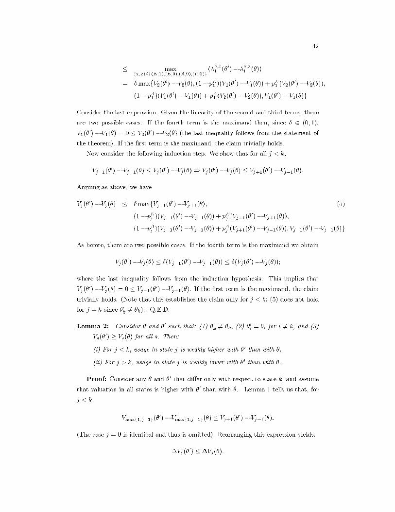
42

≤ max(a,x)∈(E,1),(E,0),(A,0),(R,0)

(λa,x1 (θ′)− λa,x1 (θ))

= δmaxV2(θ′) − V2(θ), (1− pE1 )(V1(θ

′)− V1(θ)) + pE1 (V2(θ′) − V2(θ)),

(1− pA1 )(V1(θ′) − V1(θ)) + pA1 (V2(θ

′) − V2(θ)), V1(θ′)− V1(θ)

Consider the last expression. Given the linearity of the second and third terms, there

are two possible cases. If the fourth term is the maximand then, since δ ∈ (0, 1),

V1(θ′) − V1(θ) = 0 ≤ V2(θ

′) − V2(θ) (the last inequality follows from the statement of

the theorem). If the first term is the maximand, the claim trivially holds.

Now consider the following induction step. We show that for all j < k,

Vj−1(θ′) − Vj−1(θ) ≤ Vj(θ

′)− Vj(θ)⇒ Vj(θ′)− Vj(θ) ≤ Vj+1(θ

′) − Vj+1(θ).

Arguing as above, we have

Vj(θ′) − Vj(θ) ≤ δmaxVj+1(θ

′)− Vj+1(θ), (5)

(1− pEj )(Vj−1(θ′) − Vj−1(θ)) + pEj (Vj+1(θ

′)− Vj+1(θ)),

(1− pAj )(Vj−1(θ′) − Vj−1(θ)) + pAj (Vj+1(θ

′)− Vj+1(θ)), Vj−1(θ′) − Vj−1(θ)

As before, there are two possible cases. If the fourth term is the maximand we obtain

Vj(θ′)− Vj(θ) ≤ δ(Vj−1(θ

′) − Vj−1(θ)) ≤ δ(Vj(θ′) − Vj(θ));

where the last inequality follows from the induction hypothesis. This implies that

Vj(θ′) − Vj(θ) = 0 ≤ Vj+1(θ

′) − Vj+1(θ). If the first term is the maximand, the claim

trivially holds. (Note that this establishes the claim only for j < k; (5) does not hold

for j = k since θ′

k = θk). Q.E.D.

Lemma 2: Consider θ and θ′ such that: (1) θ

′

k= θk, (2) θ

′

i= θi for i = k, and (3)

Vs(θ′) ≥ Vs(θ) for all s. Then:

(i) For j < k, usage in state j is weakly higher with θ′ than with θ,

(ii) For j > k, usage in state j is weakly lower with θ′ than with θ.

Proof: Consider any θ and θ′ that differ only with respect to state k, and assume

that valuation in all states is higher with θ′ than with θ. Lemma 1 tells us that, for

j < k,

Vmax1,j−1(θ′)− Vmax1,j−1(θ) ≤ Vj+1(θ

′) − Vj+1(θ).

(The case j = 0 is identical and thus is omitted). Rearranging this expression yields:

∆Vj(θ′) ≤ ∆Vj(θ).

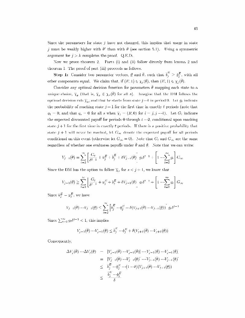
43

Since the parameters for state j have not changed, this implies that usage in state

j must be weakly higher with θ′ than with θ (see section 5.1). Using a symmetric

argument for j > k completes the proof. Q.E.D.

Now we prove theorem 2. Parts (i) and (ii) follow directly from lemma 2 and

theorem 1. The proof of part (iii) proceeds as follows.

Step 1: Consider two parameter vectors, θ and θ, such that bE

j ≥ bEj , with all

other components equal. We claim that, if (E, 1) ∈ χj(θ), then (E,1) ∈ χj(θ).

Consider any optimal decision function for parameters θ mapping each state to a

unique choice, χs (that is, χs ∈ χs(θ) for all s). Imagine that the DM follows the

optimal decision rule χs, and that he starts from state j−1 in period 0. Let gt indicate

the probability of reaching state j +1 for the first time in exactly t periods (note that

q1 = 0, and that qs = 0 for all s when χi = (R,0) for i = j, j − 1). Let Gt indicate

the expected discounted payoff for periods 0 through t − 2, conditional upon reaching

state j+1 for the first time in exactly t periods. If there is a positive probability that

state j + 1 will never be reached, let G∞ denote the expected payoff for all periods

conditional on this event (otherwise let G∞

= 0). Note that Gt and G∞

are the same

regardless of whether one evaluates payoffs under θ and θ. Note that we can write:

Vj−1(θ) =∞∑t=2

[Gt

δt−1+ uEj + b

E

j + δVj+1(θ)

]gtδ

t−1 +

[1−

∞∑t=2

gt

]G∞

Since the DM has the option to follow χsfor s < j + 1, we know that

Vj−1(θ) ≥∞∑t=2

[Gt

δt−1+ uEj + b

Ej + δVj+1(θ)

]gtδ

t−1 +

[1−

∞∑t=2

gt

]G∞

Since uEj = uEj , we have

Vj−1(θ)− Vj−1(θ) ≤∞∑t=2

[bE

j − bEj + δ(Vj+1(θ) − Vj+1(θ))

]gtδ

t−1

Since∑∞

t=2gtδ

t−1 < 1, this implies

Vj−1(θ)− Vj−1(θ) ≤ bE

j − bEj + δ(Vj+1(θ) − Vj+1(θ))

Consequently,

∆Vj(θ)−∆Vj(θ) = [Vj−1(θ)− Vj+1(θ)]− [Vj−1(θ)− Vj+1(θ)]

= [Vj−1(θ)− Vj−1(θ)]− [Vj+1(θ)− Vj+1(θ)]

≤ bE

j − bEj − (1− δ)(Vj+1(θ)− Vj+1(θ))

≤bE

j − bEj

δ

44

(where, in the last step, we have used δ < 1 along with the fact that, by theorem 1,

Vj+1(θ) ≥ Vj+1(θ)). Since, by assumption, (E, 1) ∈ χj(θ), we know that ∆Vj(θ) ≤bEj

δ.

Consequently, we have

∆Vj(θ) ≤ ∆Vj(θ) +bE

j − bEj

δ

≤bEj

δ+

bE

j − bEj

δ=

bE

j

δ

But this implies (E, 1) ∈ χj(θ).

Step 2: Consider any θ and θ with bE

j ≥ bEj and/or pEj ≤ pE

j(and all other

components equal). We claim that, if (E, x) ∈ χj(θ) for x = 0, 1, then χj(θ) = χj(θ).

It is easy to check that Vs(θ) = Vs(θ) satisfies (1) through (4) for all s when θ = θ.

Consequently, Vs(θ) is also the optimized value function with θ, and the elements of

χj(θ) maximize the expression (4) for state j with θ = θ.

Step 3: Consider any θ and θ with bE

j ≥ bEj and/or pEj ≤ pEj

(and all other

components equal). We claim that, if (E, 0) ∈ χj(θ) for x = 0, 1, then (a,0) ∈ χj(θ)

for a = A,R. Suppose on the contrary that (a, 0) ∈ χj(θ) for a ∈ A,R. Then,

arguing as in step 2, Vs(θ) = Vs(θ). It is easy to check that this implies (E,0) cannot

maximize the expression (4) for state j with θ = θ, so (E, 0) ∈ χj(θ), which is a

contradiction.

Combining steps 1, 2, and 3, we conclude that, for θ and θ with bE

j ≥ bEj (and all

other components equal), any element of χj(θ)\χj(θ) must involve less usage than any

element of χj(θ), and any element of χj(θ)\χj(θ)must involve more usage than any

element of χj(θ). Consequently, usage is (weakly) increasing in bEj .

Step 4: Consider any θ and θ that differ only with respect to pEj , uRj , and/or cj.

We claim that, if (E,1) ∈ χj(θ), then (E,1) ∈ χj(θ). This is a corollary of Theorem

3, part (i), which is proven below.

Combining steps 2, 3, and 4, we conclude that, for θ and θ with pEj ≤ pEj(and all

other components equal), any element of χj(θ)\χj(θ) must involve less usage than any

element of χj(θ), and any element of χj(θ)\χj(θ)must involve more usage than any

element of χj(θ). Consequently, usage is (weakly) decreasing in pEj .

Step 5: Consider any θ and θ with uRj ≥ uRj and/or cj ≤ cj (and all other

components equal). We claim that if (R, 0) ∈ χj(θ), then χj(θ) = χj(θ). The

argument is analogous to that given in step 2.

Step 6: Consider any θ and θ with uRj ≥ uRj and/or cj ≤ cj (and all other

components equal). We claim that if (R,0) ∈ χj(θ), then (a,0) ∈ χj(θ) for a = E,A.

The argument is analogous to that given for step 3.

Combining steps 4, 5, and 6, we conclude that, for θ and θ with uRj ≥ uRj and/or

cj ≤ cj (and all other components equal), any element of χj(θ)\χj(θ) must involve less

45

usage than any element of χj(θ), and any element of χj(θ)\χj(θ)must involve more

usage than any element of χj(θ). Consequently, usage is (weakly) decreasing in uRj

and (weakly) increasing in cj. Q.E.D.

Proof of Theorem 3

(i) Consider some θ′ for which (E, 1) ∈ χj(θ′). Suppose that θ′′ coincides with

θ′ except for pEj , pAj , u

Aj , u

Rj , b

Aj , and/or cj (subject to the restrictions imposed by

assumptions 1 and 2). We claim that (E,1) ∈ χj(θ′′). By construction, Vs(θ

′) satisfies

(1) through (4) for θ = θ′. We argue that Vs(θ′′) = Vs(θ

′) also satisfies (1) through (4)

for θ = θ′′. Under the hypothesis that Vs(θ′′) = Vs(θ

′), we have λa,xs (θ′) = λa,xs (θ′′)

for all s = j, and for (s, a, x) = (j, E,1). Thus, (4) is satisfied for all s = j. Since

(E, 1) ∈ χj(θ′) we know that (E,1) maximizes (4) for state j with θ = θ′, which is

equivalent to ∆Vj(θ′) ≤

bEjδ. But then, under our hypothesis, ∆Vj(θ

′′) ≤bEjδ

as well,

so (E, 1) remains a maximizer for state j with θ = θ′′. Since λE,1s

(θ′) = λE,1s (θ′′), the

maximized value of (4) is unchanged with θ = θ′′. Accordingly, Vs(θ′′) = Vs(θ

′) is

the maximized value function when θ = θ′′, and χj(θ′′) is the set of optimal choices in

state j.

(ii) Consider some θ for which (R,0) ∈ χn(θ). Construct some θ′ by increasing the

values of pakor ck, or by decreasing the values of ba

kor ua

k, for some k > n. By theorem

2 part (i), (R,0) ∈ χn(θ). Consider the optimization problem formed by restricting

the model to addictive states 0 through n, and imposing the action (R, 0) in state n.

This problem has the same solution as the complete problems with either θ or θ′ on

states 0 through n since conditions (1) to (4) coincide on these states. It follows that

the optimal solution at θ′ remains unchanged for states 0 through n.

(iii) The proof is analogous to that of part (ii). Q.E.D.

Proof of Theorem 4

Step 1. We show that V0(θ) ≥ V1(θ). Since (E, 1) is an option at s = 0, we

have that V0(θ) ≥ uE0+ bE

0+ δV1(θ). Furthermore, since the substance is destructively

addictive, we must have that V1(θ) ≤uE

1+bE

1

1−δ≤

uE

0+bE

0

1−δ. These two inequalities imply

that V0(θ) ≥ (1− δ)V1(θ) + δV1(θ) = V1(θ).

Step 2 Now we show that Vs−1(θ) ≥ Vs(θ) implies Vs(θ) ≥ Vs+1(θ). We consider

four cases. These cases are not mutually exclusive, but they are exhaustive.

(i) (E, 1) ∈ χs(θ). In this case, Vs(θ) = uEs+ bE

s+ δVs+1(θ). Furthermore, since

states lower than s are never reached (once the DM is in state s), and the substance is

destructively addictive, we have that Vs+1(θ) ≤uE

s+b

E

s

1−δ. The argument then proceeds

as in step 1.

(ii) (R, 0) ∈ χs+1(θ). In this case we have that

Vs+1(θ) = uRs+1 − cs+1 + δVs(θ) ≤ uE

s+ bE

s+ δVs(θ).

46

Also, Vs(θ) ≥ uEs+ bE

s+ δVs+1(θ) since (E,1) is an option at state s. This implies that

Vs(θ) ≥ Vs+1(θ)− δVs(θ) + δVs+1(θ) and thus Vs(θ) ≥ Vs+1(θ).

(iii) (E,1) ∈ χs+1(θ). In this case Vs+1(θ) ≤uE

s+1+bE

s+1

1−δ≤

uE

s+b

E

s

1−δ, so uE

s+ bE

s≥

(1− δ)Vs+1(θ). Also, at state s we have that Vs(θ) ≥ uEs+ bE

s+ δVs+1(θ) (since (E,1)

is available as an option). Combining these inequalities yields Vs(θ) ≥ Vs+1(θ).

(iv) Two conditions hold: (a) either (E, 0) ∈ χs+1(θ) or (A,0) ∈ χs+1(θ), and (b)

(E, 1) ∈ χs(θ). Consider a such that (a,0) ∈ χs+1(θ). Since bEs+1 ≥ 0, we must have

Vs(θ) ≥ Vs+2(θ) (otherwise (E, 1) would be preferable to (a,0) at s + 1). Suppose,

towards a contradiction, that Vs+1(θ) > Vs(θ). Then Vs+1(θ) > Vs+2(θ). Then we

have that

Vs+1(θ) = pas+1(u

a

s+1 + bas+1 + δVs+2(θ)) + (1− pa

s+1)(ua

s+1 + δVs(θ))

≤ pas+1(u

a

s+1 + bas+1 + δVs+1(θ)) + (1− pa

s+1)(ua

s+1 + δVs−1(θ))

≤ pas+1(u

a

s+ ba

s+ δVs+1(θ)) + (1− pa

s+1)(ua

s+ δVs−1(θ))

≤ pas(ua

s+ ba

s+ δVs+1(θ)) + (1− pa

s)(ua

s+ δVs−1(θ)) (see below)

≤ Vs(θ),

which is a contradiction. The third inequality follows because (E,1) ∈ χs(θ), which

requires ∆Vs(θ) ≥bE

s

δ, which in turn implies uas + δVs−1(θ) ≥ u

a

s+ b

a

s+ δVs+1(θ).

Step 3 At s = 0 the DM can guarantee himself a constant payoffuA

o

1−δ, which implies

that ∆V0(θ) ≥ 0. By the conditions in section 5.1, it follows that (E,1) ∈ χ0(θ) when

bE0< 0. Q.E.D.

Proof of Theorem 5

Let Ts(σ) denote the lump-sum tax (possibly negative) that the DM pays in state

s with the tax-subsidy scheme σ. We claim that, if the DM follows χs(θ(σ)) when

the parameter vector is θ(0), he achieves an expected discounted payoff in each state s

of Vs(θ(σ)). From this it follows immediately that the optimized value function with

θ(0) satisfies Vs(θ(0)) ≥ Vs(θ(σ)), as required, with strict inequality if no member of

χs(θ(σ)) is optimal with the parameter vector θ(0).

To establish the claim, suppose that the DM selects a decision rule (ζ,ψ) with

(ζs, ψs) ∈ χs(θ(σ)) for all s. Government budget balance (with no redistributions

between addictive states) requires Ts(σ) = σζss . If ζs = E or A, then with tax-subsidy

scheme σ the choice (ζs, ψs) confers instantaneous utility in state s of

uζss (σ) +ψsbζs

s (σ) = ws(ys −ψsq − Ts(σ) + σζss , ψs, ζs)

= ws(ys −ψsq,ψs, ζs)

= uζss (0) + ψsbζss (0)

47

Similarly, if ζs = R, then with tax-subsidy scheme σ the choice (ζs, ψs) confers instan-

taneous utility in state s of

uRs (σ)− cs(σ) = ws(ys − Ts(σ)− rs + σRs , 0, R)

= ws(ys − rs,0,R)

= uRs (0)− cs(0)

It follows that the decision rule (ζ, ψ) generates the same expected discounted utility

in all states with σ as with no tax-subsidy scheme. Q.E.D.

Proof of Theorem 6

Let Ts(τ ) denote the lump-sum payment (possibly negative) that the DM pays in

state s with the tax-subsidy τ . We claim that, if the DM follows χs(θ(τ )) when the

parameter vector is θ(0), he achieves an expected discounted payoff in each state s

of no less than Vs(θ(τ)). From this it follows immediately that the optimized value

function with θ(0) satisfied Vs(θ(0)) ≥ Vs(θ(τ )), as required, with strict inequality if

no member of χs(θ(σ)) is optimal with parameter vector θ(0).

To establish the claim, suppose that the DM selects a decision rule (ζ,ψ) with

(ζs, ψs) ∈ χs(θ(τ )) for all s. Government budget balance (with no redistributions

between addictive states) requires Ts(σ) =(ψs + (1− ψs)p

ζss

)τ when ζs = E or A,

and Ts(σ) = 0 when ζs = R.

If (ζs, ψs) = (E,1), then with tax-subsidy τ the choice (E,1) confers instantaneous

utility in state s of

uEs (τ ) + bEs (τ ) = ws(ys − (q + τ ) + Ts(τ ),1,E)

= ws(ys − q,1, E)

= uEs (0) + bEs (0)

If (ζs, ψs) = (R,0), then with tax-subsidy τ the choice (R,0) confers instantaneous

utility in state s of

uEs (τ )− cs(σ) = ws(ys − rs + Ts(τ ), 0, E)

= ws(ys − rs, 0, E)

= uRs (0) − cs(0)

If (ζs, ψs) = (a,0) with a = E or A, then with tax-subsidy τ the choice (a,0) confers

instantaneous utility in state s of

uas(τ) + pasbas(τ ) = pasws(ys − (q + τ ) + Ts(τ ),1, a) + (1− pas)ws(ys + Ts(τ),0, a)

48

= pasws(ys − (q + τ ) + pasτ, 1, a) + (1− pas)ws(ys + pasτ, 0, a)

= pasws(ys − q, 1, a) + (1− pas)ws(ys,0, a) +Ω

= uas (0) + pasbas(0) + Ω

where

Ω = (1− pas)

∫ pa

sτ

0

∂ws(ys + z, 0, a)

∂edz − pa

s

∫0

−(1−pas)τ

∂ws(ys − q + z, 1, a)

∂edz

Now suppose that ∂ws(e,0,a)∂e

≤∂ws(e,1,a)

∂e(as in part (i) of the theorem). Imagine

that τ > 0. Since ws(e, x, a) is concave in e,

Ω ≤ (1− pas)

∫pa

sτ

0

∂ws(ys + z, 1, a)

∂edz − p

a

s

∫0

−(1−pas)τ

∂ws(ys − q + z, 1, a)

∂edz

≤ (1− pas)

∫pa

sτ

0

∂ws(ys − q + z,1, a)

∂edz − pa

s

∫0

−(1−pas)τ

∂ws(ys − q + z, 1, a)

∂edz

= (1− pas)ws(ys − q + pasτ,1, a) + pasws(ys − q − (1− pas)τ,1, a) −ws(ys − q,1, a)

≤ 0,

where the last inequality uses concavity and the fact that (1−pas)(ys−q+pasτ )+pas(ys−

q− (1− pas)τ ) = ys − q. Thus, for all states, the choice (ζs, ψs) confers weakly greater

instantaneous utility with no tax than with the tax. It follows that the decision rule

(ζ, ψ) generates weakly greater expected discounted utility in all states with no tax

than with τ > 0.

Finally, suppose that ∂ws(e,0,a)∂e

≥∂ws(e−q,1,a)

∂e(as in part (ii) of the theorem).

Imagine that τ < 0. Then

Ω ≤ pas

∫−(1−pa

s)τ

0

∂ws(ys + z,0, a)

∂edz − (1− pa

s)

∫0

pasτ

∂ws(y

s+ z,0, a)

∂edz

= pasws(y

s− q − (1− pa

s)τ,1, a) + (1− pa

s)w

s(y

s− q + pa

sτ,1, a) −w

s(y

s− q,1, a)

≤ 0,

As before, it follows that the decision rule (ζ, ψ) generates weakly greater expected

discounted utility in all states with no subsidy than with τ < 0. Q.E.D.

49

References

[1] Abratt, R. and S. Goodey (1990) “Unplanned Buying and In-Store Stimuli in

Supermarkets,” Managerial and Decision Economics,” 111-21.

[2] Barkow, Jerome, Leda Cosmides, and John Tooby (1995) The Adapted Mind :

Evolutionary Psychology and the Generation of Culture.Oxford: Oxford University

Press.

[3] Becerra, Lino, Hans Breiter, Roy Wise, Gilberto Gonzalez, and David Borsook

(2001) “Reward Circuitry and Activation by Noxious Thermal Stimuli,” Neuron,

32:927-46.

[4] Bechara, A., A. Damasio, H. Damasio, and S. Anderson (1994) “Insensitivity to

Future Consequences Following Damage to Human Prefrontal Cortex,” Cognition,

7-15.

[5] Bechara, A., D. Tranel, A. Damasio, and H. Damasio (1996) “Failure to Respond

Autonomically to Anticipated Future Outcomes Following Damage to the Pre-

frontal Cortex,” Cerebral Cortex, 215-25.

[6] Bechara, A., D. Tranel, A. Damasio, and H. Damasio (1997) “Deciding Advante-

geously Before Knowing the Advantageous Strategy,” Science, 1293-95.

[7] Becker, Gary and Kevin Murphy (1988) “A Theory of Rational Addiction,” Jour-

nal of Political Economy, 96(4), 675-700.

[8] Berke, J.D. and S. E. Hyman (2000) “Addiction, Dopamine, and the Molecular

Mechanisms of Memory,” Neuron, 25: 515-32.

[9] Bernheim, Douglas and Antonio Rangel (2002) “Cognition, Evaluation, and He-

donics: A Brain Processes Model of Decision-Making”, Stanford manuscript.

[10] Berridge, K. (1996) “Food Reward: Brain Substrates of Wanting and Liking,”

Neuroscience and Biobehavioral Reviews, 20(1):1-25

[11] Berridge, K. (1999) “Pleasure, Pain, Desire, and Dread: Hidden Core Processes of

Emotion,” in Well-Being: The Foundations of Hedonic Pscyhology, D. Kaheman,

E. Diener, and N. Schwarz (eds.), 525-57

[12] Berridge, Kent, and Terry Robinson (1998) “What is the role of dopamine in

reward: hedonic impact, reward learning, or incentive salience?”, Brain Research

Review, 28:309-69.

[13] Breiter, Hans C., et. al. (1997) “Acute Effects of Cocaine on Human Brain Activity

and Emotion,” Neuron, 19:591-611.

50

[14] Center for Disease Control (1993), “Smoking-Attributable Mortality and Years of

Potential Life Lost - United States, 1990,”Morbidity and Mortality Weekly Report,

42(33), 645-8.

[15] Chaloupka, F. and K. Warner (2001) “The Economics of Smoking”, in J. Newhouse

and D. Cutler (eds.), Handbook of Health Economics, North-Holland.

[16] Damasio, Antonio (1994) Descartes Error: Emotion, Reason, and the Human

Brain. New York: Putnam.

[17] Davis, M. (1992a) “The Role of the Amygdala in Fear and Anxiety,” Annual

Review of Neuroscience, 353-75.

[18] Davis, M. (1992b) “The Role of the Amygdala in Conditioned Fear,” In J.P.

Aggleton (ed.), The Amygdala: Neurobiological Aspects of Emotion, Memory, and

Mental Disfunction, New York: Wiley-Liss.

[19] Gardner, Eliot and James David (1999) “The Neurobiology of Chemical Addic-

tion,” in Getting Hooked: Rationality and Addiction, edited by Jon Elster and

Ole-Jorgen Skog. Cambridge: Cambridge University Press.

[20] Gawin, F.H. (1991) “Cocaine addiction: Psychology and neurophysiology,” Sci-

ence, 1580-6.

[21] Gazzaniga, M. (1990). Transcript of interview published in the National Review.

[22] Gazzaniga, M. (1994). Transcript of interview published in the National Review.

[23] Gerstein, Dean, et. al. (1999). Gambling Impact and Behavior Study, Report to

the National Gambling Impact Study Commission. Chicago, IL: National Opinion

Research Center.

[24] Goldstein, A. (2001) Addiction: From Biology to Drug Policy. Second Edition.

New York: Oxford University Press.

[25] Goldstein, A. and H. Kalant (1990) “Drug Policy: Striking the Right Balance,”

Science 249: 1513-21.

[26] Gruber, Jonathan, and Botond Koszegi (2001) “Is Addiction “Rational”? Theory

and Evidence,” Quarterly Journal of Economics, 116(4): 1261-1303 .

[27] Gul, Faruk and Wolfgang Psendorfer (2001a), “Temptation and Self-Control”,

Econometrica 69(6): 1403-35.

[28] Gul, Faruk and Wolfgang Psendorfer (2001b) “A Theory of Addiction,” Princeton

mimeo.

51

[29] Harris, J.E. (1993) Deadly Choices: Coping with Health Risks in Everyday Life.

New York: Basic Books.

[30] Helmuth, L. (2001) “Beyond the Pleasure Principle,” Science, 294:983-84.

[31] Holden, C. (2001a) “‘Behavioral’ addictions: Do they exist?” Science, 294:980-82.

[32] Holden, C. (2001b) “Zapping Memory Centers Triggers Drug Craving,” Science,

292:1039

[33] Hser, Y.I., D. Anglin, and K. Powers (1993) “A 24-year follow-up study of Cali-

fornia narcotics addicts,” Archives of General Psychiatry, 50:577-84.

[34] Hser, Y.I., V. Hoffman, C. Grella, and M.D. Anglin (2001) “A 33 year follow-up

of narcotics addicts,” Archives of General Psychiatry, 58:503-8.

[35] Hung, Angela (2000) “A Behavioral Theory of Addiction,” Caltech, manuscript.

[36] Janis, I. (1967) “Effects of fear arousal on attitudinal change,” Advances in Ex-

perimental Psychology, 167-224.

[37] Hyman, Steven and Robert Malenka [2001] “Addiction and the Brain: The Neu-

robiology of Compulsion and Its Persistence,” Nature Reviews: Neurosience, 2:

695-703.

[38] Koob, G. and M. LeMoal (1997) “Drug Abuse: Hedonic Homeostatic Dysregula-

tion”, Science 278, October, 52-8.

[39] Laibson, David (1997) “Golden Eggs and Hyperbolic Discounting,” Quarterly

Journal of Economics, (112):443-77.

[40] Laibson, David (2001) “A Cue-Theory of Consumption,” Quarterly Journal of

Economics, 116(1): 81-120.

[41] LeDoux, Joseph (1992) “Emotion and the Amygdala.” In J.P. Aggleton (ed.) The

Amygdala: Neurobiological Aspects of Emotion, Memory and Mental Dysfunction,

pp. 339-51. New York: Wiley-Liss.

[42] LeDoux, Joseph (1993) “Emotional Networks in the Brain,” In Michael Davis

and Jeannette Haviland (eds.), Handbook of Emotions, New York: The Guildford

Press.

[43] LeDoux, Joseph (1998) The Emotional Brain : The Mysterious Underpinnings of

Emotional Life. Touchstone books.

[44] Loewenstein, George (1996) “Out of Control: Visceral Influences on Behavior,”

Organizational Behavior and Human Decision Processes, 65(3) 272-92.

52

[45] Loewenstein, George (1999) “A Visceral Account of Addiction,” in Jon Elster and

Ole-Jorgen Skog (eds.) Rationality and Addiction. Cambridge: Cambridge Univer-

sity Press.

[46] Loewenstein, George, and Jennifer S. Lerner (2001) “The Role of Affect in Decision

Making,” in R.J. Davidson, H.H. Goldsmith, and K.R. Scherer (eds.) Handbook of

Affective Science. Oxford: Oxford University Press.

[47] Loewenstein, George, Ted O’Donoghue, and Matthew Rabin (2000) “Projection

Bias in Predicting Future Utility,” mimeo.

[48] Massing, Michael. The Fix. Los Angeles: University of California Press, 2000.

[49] MacCoun, R. and P. Reuter (2001) Drug War Heresies: Learning from Other

Vices, Times, and Places. Cambridge University Press.

[50] Metcalfe, Janet, and Walter Mischel (1999) “AHot/Cool-System Analysis of Delay

of Gratification: Dynamics of Willpower,” Psychological Review, 106(1):3-19.

[51] Miron, J. and J. Zwiebel (1995) “The Economic Case Against Drug Prohibition,”

Journal of Economic Perspectives, 9(4):175-92.

[52] Mischel, W. (1974) “Processes in delay of gratification,” In Advances in Experi-

mental Social Psychology, volume 7, D. Berkowitz editor, 249-272.

[53] Mischel, W. and B. Moore (1973) “Cognitive Appraisals and Transformations in

the Delay of Gratification,” Journal of Personality and Social Psychology, 28:172-9.

[54] Michel, W., Y. Shoda, and M. Rodriguez (1992) “Delay of Gratification in Chil-

dren,” in Choice over Time, G. Loewenstein and Jon Elster editors, New York:

Rusell Sage.

[55] National Institute on Alcohol Abuse and Alcoholism (2001), “Economic Perspec-

tives in Alcholism Research”, Alcohol Alert, National Institutes of Health, No.

51.

[56] National Institute on Drug Abuse (1998). The Economic Costs of Alcohol and

Drug Abuse in the United States, 1992. Bethesda, MD: National Institutes of

Health (NIH Publication Number 98-4327).

[57] Nestler, E.J. (2001) “Molecular Basis of Long-term Plasiticity Underlying Addic-

tion”, Nature Reviews Neuroscience, 2:119-28.

[58] O’Brien, C. (1976) “Experimental analysis of conditioning factors in human nar-

cotic addiction,” Pharmacological Review, 25:533-43.

53

[59] O’Brien, C. (1997) “A Range of Research-Based Pharmacotherapies for Addic-

tion,” Science, 278:66-70.

[60] O’Donoghue, Ted, and Mathew Rabin (1999), “Doing It Now or Later,” American

Economic Review, (89):103-24.

[61] O’Donoghue, Ted, and Mathew Rabin (2000), “Addiction and Present-Biased

Preferences,” manuscript, Berkeley.

[62] Office of National Drug Control Policy (2001a). What American Users Spend on

Illegal Drugs.Washington, DC: Executive Office of the President (Publication No.

NCJ-192334).

[63] Office of National Drug Control Policy (2001b). The Economic Costs of Drug

Abuse in the United States, 1992-1998. Washington, DC: Executive Office of the

President (Publication No. NCJ-190636).

[64] Olds, J. and P. Milner (1954) “Positive reinforcement produced by electrical stim-

ulation of septal area and other regions of rat brain,” Journal of Comparative and

Physiological Psychology, 419-27.

[65] Orphanides, Athanasios, and David Zervos (1995) “Rational Addiction with

Learning and Regret,” Journal of Political Economy, 103: 739-58.

[66] Panksepp, J. (1998) Affective Neuroscience: The Foundations of Human and An-

imal Emotions. New York: Oxford University Press.

[67] Pickens, R. and W.C. Harris (1968) “Self-administration of d-amphetamine by

rats,” Pscyhopharmacologia, 158-63.

[68] Robins, L. (1994) “Vietnam Veterans’ Rapid Recovery from Heroin Addiction: a

Fluke or Normal Expectation,” Addiction, 1041-54.

[69] Robins, L., D. Davis, and D. Goodwin (1974) “Drug Use by U.S. Army Enlisted

Men in Vietnam: a Follow-up on their Return Home,” American Journal of Epi-

demiology, 235-49.

[70] Robinson. T. and K. Berridge (1993) “The Neural Basis of Drug Craving: An

Incentive-Sensitization Theory of Addiction,” Brain Research Reviews, 18(3):247-

91.

[71] Robinson, T. and K. Berridge (2000) “The psychology and neurobiology of addic-

tion: an incentive sensitization view,” Addiction, Suppl 2:91-117.

[72] Schultz, W. (1998) “Predictive reward signal of dopamine neurons,” Journal of

Neurophysiology, 80:1-27.

54

[73] Schultz, Wolfram (2000) “Multiple Reward Signals in the Brain,”Nature Reviews

Neurosicence, 1:199-207.

[74] Schultz, W., P. Dayan, and P.R. Montague (1997) “A neural substrate of prediction

and reward,” 275:1593-99.

[75] Trosclair, A., C. Huston, L. Pederson, and I. Dillon (2002), “Cigarette Smoking

Among Adults — United States, 2000,” Morbidity and Mortality Weekly Report,

51(29), 642-645.

[76] Ungless, M., J. Whistler, R. Malenka, and A. Bonci (2001) “Single cocaine ex-

posure in vivo induces long-term potentiation in dopamine neurons,” Nature,

411(31):583-87.

[77] United States Census Bureau (2001). Statistical Abstract of the United States.

Washington, DC: US Government Printing Office.

[78] Volkow, N.D. (1997) “The role of the dopamine system in addiction,” Hospital

Practice (Special reports), April: 22-26.

[79] Volkow, N.D., Wang, G.-J., Fowler, J.S. (1997) “Imaging studies of cocaine in the

human brain and studies of the cocaine addict. In: Imaging Brain Structure and

Function, ” in Annals of the New York Academy of Sciences, Lester D.S., Felfer

C.C., Lewis E.N. (eds), 820:41-53.

[80] Vorel, S. and E. Garner (2001) “Drug Addiction and the Hyppocampus,” Science,

294(9):1235a

[81] Vorel, S., et. al. (2001) “Relapse to Cocaine-Seeking After Hippcampal Theta

Burst Stimulation,” Science, 292:1175-78.

[82] Wegner, Daniel (1994) White Bears and other unwanted thoughts: Suppression,

obsession, and the psychology of mental control. New York: Guildford Press.

[83] Wickelgren (1997) “Getting the Brain’s Attention,” Science, 278:35-37.

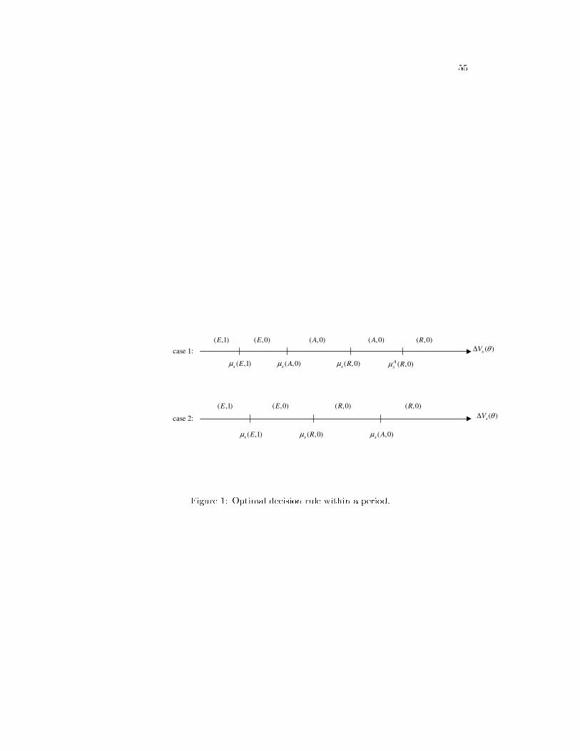
55

case1:

( )sV θ∆

( )sV θ∆

case2:

( ,1)s Eµ

( ,1)s Eµ

( ,0)s Aµ

( ,0)s Aµ

( ,0)s Rµ

( ,0)s Rµ ( ,0)As Rµ

( ,1)E

( ,1)E

( ,0)E

( ,0)E ( ,0)A( ,0)A

( ,0)R

( ,0)R

( ,0)R

Figure 1: Optimal decision rule within a period.

56

s

( )sV θ

( ,1)E( ,1)E ( ,0)E( ,0)E( ,0)E ( ,0)A( ,0)A ( ,0)R( ,0)R ( ,0)E ( ,1)E( ,1)E

s

( )sV θ∆

( ,1)E

( ,0)E

( ,0)A

( ,0)R

0 1 2 3 4 5 6 7 8 9 10 11

0 1 2 3 4 5 6 7 8 9 10 11

Figure 2: Graphical representation of the optimal decision rule.