IT 16009

Examensarbete 30 hpFebruari 2016

Clustering Multilayer Networks

Nazanin Afsarmanesh Tehrani

Institutionen för informationsteknologiDepartment of Information Technology

Teknisk- naturvetenskaplig fakultet UTH-enheten Besöksadress: Ångströmlaboratoriet Lägerhyddsvägen 1 Hus 4, Plan 0 Postadress: Box 536 751 21 Uppsala Telefon: 018 – 471 30 03 Telefax: 018 – 471 30 00 Hemsida: http://www.teknat.uu.se/student

Abstract

Clustering Multilayer Networks

Nazanin Afsarmanesh Tehrani

Detecting community structure is an important methodology to study complexnetworks. Community detection methods can be divided into two main categories:partitioning methods and overlapping clustering methods. In partitioning methods,each node can belong to at most one community while overlapping clusteringmethods allow communities with overlapping nodes as well. Community detection isnot only a problem in single networks today, but also in multilayer networks whereseveral networks with the same participants are considered at the same time. Inrecent years, several methods have been proposed for recognizing communities inmultilayer networks; however, none of these methods finds overlapping communities.On the other hand, in many types of systems, this approach is not realistic. Forexample, in social networks, individuals communicate with different groups of people,like friends, colleagues, and family, and this determine overlaps between communities,while they also communicate through several networks like Facebook, Twitter, etc.

The overall purpose of this study was to introduce a method for finding overlappingcommunities in multilayer networks. The proposed method is an extension of thepopular Clique Percolation Method (CPM) for simple networks. It has been shownthat the structure of communities is dependent on the definition of cliques inmultilayer networks which are the smallest components of communities in CPM, andtherefore, several types of communities can be defined based on different definitionsof cliques. As the most conventional definition of communities, it is necessary for allnodes to be densely connected in single networks to form a community in themultilayer network. In the last part of the thesis, a method has been proposed forfinding these types of communities in multilayer networks.

Tryckt av: Reprocentralen ITCIT 16009Examinator: Edith NgaiÄmnesgranskare: Michael AshcroftHandledare: Matteo Magnani

1

Contents

1 Introduction .............................................................................................................................. 4 1.1 Introduction ........................................................................................................................ 4

1.2 Thesis Objective .................................................................................................................. 5

2 Background ............................................................................................................................... 6

2.1 Introduction ........................................................................................................................ 6

2.2 Local Definitions ................................................................................................................. 7

2.2.1 Definitions Based on Internal Cohesion ..................................................................... 8

2.2.2 Definitions Based on Comparison of Internal and External cohesion ..................... 9

2.3 Definitions based on vertex similarity ............................................................................ 11

2.4 Global definitions and quality functions ......................................................................... 12

2.4.1 Modularity .................................................................................................................. 13

2.5 Clustering Methods for Simple Networks ....................................................................... 14

2.5.1 Graph Partitioning Methods ...................................................................................... 15

2.5.2 Spectral Clustering Methods ..................................................................................... 19

2.5.3 Hierarchical Clustering .............................................................................................. 20

2.5.4 Divisive Clustering and Algorithm of Girvan and Newman .................................... 21

2.5.5 Modularity-­‐‑Based Methods ....................................................................................... 22

2.5.6 Overlapping Community Detection Methods .......................................................... 23

3 Multilayer Networks and Clustering Methods ................................................................. 24

3.1 Introduction ...................................................................................................................... 24

3.1.1 Merging the Layers .................................................................................................... 25

3.2 Clustering Multi-­‐‑Layer Networks .................................................................................... 25

3.2.1 Converting to Single Networks ................................................................................. 26

3.2.2 Methods with Spectral Perspective .......................................................................... 27

3.2.3 Modularity Based Methods ....................................................................................... 28

2

3.2.4 Other Methods............................................................................................................ 28

4 Multilayer Networks and Overlapping Communities ..................................................... 30

4.1 Introduction ...................................................................................................................... 30

4.2 Clique Percolation Method (CPM) for Simple Networks ............................................... 31

4.3 CPM for Multilayer Networks .......................................................................................... 32

4.4 Different Types of Cliques in Multilayer Networks ........................................................ 32

4.5 Maximal cliques ................................................................................................................ 34

4.6 A Comparison between Different Types of Cliques ........................................................ 34

4.7 Less Strict Constraints and Quasi Cliques ....................................................................... 36

5 Clique Based Communities in Multilayer Networks ....................................................... 38

5.1 Introduction ...................................................................................................................... 38

5.1.1 Adjacency of Cliques and Clique Based Communities ............................................ 38

5.1.2 Node Based Adjacency and Communities ................................... 39

5.1.3 Type Based Adjacency and Communities .......................... 39

5.1.4 Additional Constraints and ( ) Communities.............. 40

5.2 Communities Based on Different Types of Cliques ........................................................ 40

5.2.1 Type (1) Cliques ......................................................................................................... 41

5.2.2 Type (1) Quasi Cliques .............................................................................................. 44

5.2.3 Type (2) Cliques ......................................................................................................... 45

5.2.4 Type (2) Quasi Cliques .............................................................................................. 48

5.2.5 Type (3) Cliques........................................................................................................ 49 5.2.6 Type (3) Quasi Cliques .............................................................................................. 51

5.2.7 Type (4) Cliques ......................................................................................................... 51

5.3 Comparison between Different Types of Communities from Theoretical Aspects ..... 52

5.4 Different Types of Communities in Practice ................................................................... 53

6 CPM for Multilayer Networks ............................................................................................. 55

6.1 Introduction ...................................................................................................................... 55

6.2 Original CPM in Practice ................................................................................................... 55

6.3 CPM for Multilayer Networks .......................................................................................... 57

6.3.1 Locating the Cliques ................................................................................................... 58

6.3.2 Adjacent Cliques and Clique-­‐‑Clique Adjacency Matrix ........................................... 60

3

6.3.3 From Adjacent Cliques to Communities ................................................................... 63

6.4 Conclusion ......................................................................................................................... 67

6.3.3 Future Work ............................................................................................................... 68

Appendix A .................................................................................................................................. 69

Bibliography ............................................................................................................................... 72

4

Chapter 1

Introduction

1.1 Introduction Community detection is an important field in network science. In network analysis, each network is represented as a graph, and community detection is equivalent to clustering the vertices of the graph. A brief introduction to graph theory has been brought in Appendix A. One of the main applications of graph clustering is discovering strongly connected individuals in social networks. As a result of significant work in modern network science, many methods have been defined for community detection. Due to the growing number of social networks, community detection is not only of interest in single networks, but also in multiplex networks where several networks are considered at the same time. Multiplex networks are represented as multi-graphs, where multiple edges represent multiple relationships originating from different networks. To simplify this representation, each network can also be considered separately as a single layer in a multi-layer network, where the nodes which are repeated in different layers are considered as correlated nodes.

Community detection in multilayer networks is a new field of study which has attracted scientists and researchers in recent years. Similar to simple networks, there is no unique definition of communities in multilayer networks. Due to the complex

5

structure of multilayer networks and existence of different types of links, communities should be defined precisely before designing any clustering method. Recent methods are generalizations of the old methods based on the specific definition of communities in multilayer networks. Most of these methods try to find a set of non-overlapping communities where the resulted communities do not share any vertex.

1.2 Thesis Objective For the thesis project, clustering multilayer networks is considered as the field of study. The focus would be on overlapping communities where the resulted communities are allowed to have common vertices. Such communities should be first defined precisely. At the next step, I would try to generalize a community detection method for simple network to the multilayer one based on the corresponding definition of communities.

6

Chapter 2

Background

2.1 Introduction As a general definition, it is said that a network has a community structure if the nodes of the network can be grouped into proper sets such that nodes inside each group are densely connected. These groups are called communities or clusters, and the corresponding methods are called community detection methods or clustering methods. The communities can be both overlapping or non-overlapping. In the case of overlapping communities, the connections between different communities should be relatively sparse. In general, for a given community, the internal connections are denser than external connections. Networks with community structure have sparse graphs;; in other words, the number of edges should be of the order of the number of vertices [1]. In addition, in contrast to a network with a random structure, where the distribution of edges among the vertices is uniform and most vertices have equal or similar degree, a graph with community structure usually has vertices with both low and large degrees. It should be mentioned that a network without a community structure might still include communities. In such networks, communities do not probably cover the whole network or there is a great amount of overlapping between communities.

7

As we know, networks are represented by graphs where nodes represent entities and edges represent the relations between different entities. Community detection in a network is equivalent to clustering the graph of the network to different set of nodes or clusters. Clustering the graph into non-overlapping groups is called partitioning. For overlapping communities, the term is used rather than partition. To find communities or clusters in a network, a quantitative definition of communities should be first specified. There are many different quantitative definitions, and each definition considers different properties of communities. Each clustering algorithm is based on one of these definitions. It should be noted that final communities are just products of these algorithms and not necessarily match all properties of any definition. There are three main classes of definitions: local definitions, global definitions and definitions based on vertex similarity [1]. In the following three sections, these classes of definitions are first explained. The material and definitions have Santo fortunato [1]. Then in next sections, different types of community detection methods for simple networks are introduced.

2.2 Local Definitions Local definitions focus on individual communities as independent entities;; in other words, the strength of a community is specified by its own characteristics independent from the strength of other possible communities in the graph. Each community is considered as a subgraph and the quality of the communities is specified by the internal and external cohesions of the subgraph while the rest of the graph is neglected. There are two main types of local definitions. In the first type, a community is defined by a criterion based on the internal cohesion. The objective is finding maximal subgraphs that fulfill these criteria, so communities found by these definitions have a denser internal cohesion than external cohesion. However, the external cohesion might be still strong and by making these criteria stricter, the external cohesion can become denser. Therefore, these types of definitions cannot usually reveal much about the community structure of the network considering the external cohesions in that area. The second types of definitions define a community based on the relation between internal and external cohesions. When these criteria become strict enough, they can reveal information about community structure in that area, considering the external cohesion.

Suppose that C is a subgraph of where and . By internal edges of C we refer to those edges whose both sides are in C , and by external edges of C we

8

refer to those edges which connect a vertex in C to the rest of the graph. For each vertex in C , the internal degree of denoted by is the number of edges connecting v to other vertices in C and the external degree of denoted by is the number of edges connecting to the rest of the graph. The -

of the subgraph C is the ratio between the number of internal edges of C and the number of all possible internal edges:

Similarly, the - is ratio between the number of inter-cluster edges of C and the number of all possible inter-cluster edges:

2.2.1 Definitions Based on Internal Cohesion Internal Density

For a subgraph C to be a proper cluster or community, it is expected that its internal density be large enough. Communities can be defined assigning a minimum

threshold like for .

Complete Mutuality

A community might be defined as a group where all members are directly connected. This strict rule might be of interest in different situations, like in social networks where it might be required for members in each community to be all friends with each other. Considering the graph of the network, such a community corresponds to a maximal clique;; the largest subset of nodes where the induced subgraph is complete. In real examples, like in social networks, small cliques like triangles or 4-cliques might be frequent but larger cliques are usually rare. Therefore, it would be beneficial to relax the definition of communities, and searching for clique-like subgraphs instead of real cliques. As an example, it might be required that the distance between each two vertices be smaller than a specific value rather than being directly connected. This property is related to reachability.

9

Reachability

An -clique is a subgraph where the distance (see Appendix A.4) between each pair of its vertices in not larger than [2]. This definition is less strict than that of cliques, but it has also some problems. First, the shortest path between two vertices in an -clique can include vertices which are not in that -clique. Therefore, the diameter (see Appendix A.4) of an -clique might be larger than n. Furthermore, an n-clique might be disconnected which contradicts the basic property of communities. An -clan is an -clique whose diameter is not larger than [3]. In other words, an -clan is a subgraph where the shortest path between each pair of its vertices within that subgraph is not larger than

Vertex Degree

Another criterion for internal cohesion is to consider a constraint for internal degree of the vertices. In other words, each vertex inside the subgraph should be adjacent to a minimum number of other vertices in that subgraph. A -plex is a maximal connected subgraph (see Appendix A.5) where each vertex of the subgraph is adjacent to other vertices in the subgraph except at most of them [4]. Similarly, a -core is a maximal connected subgraph where each of the vertices is adjacent to at least other vertices inside the subgraph [5]. Similar to a -core, we have the concept of quasi-cliques. For a graph , a subgraph of like and a constant , it is said that is a -quasi-clique in if each vertex in is directly connected to at least

of other vertices in where [6]. This is a stricter rule than that of -cliques as it imposes the existence of many internal edges.

2.2.2 Definitions Based on Comparison of Internal and

External cohesion What have been mentioned so far are criteria for internal cohesion of communities. Although internal cohesion is an important property for communities, it cannot be a basis to define communities individually. In fact, a community should have a weak cohesion to the rest of the network as well as being cohesive internally. In this section, possible criteria on external cohesions are reviewed.

10

Internal Density versus External Density

The relation between internal and external cohesions of a subgraph can determine how strong that subgraph is as a community. A subgraph is said to be a strong community if the internal degree of all of its vertices is greater than their external degree [7]. This constraint is quite strict. A more flexible constraint comes in the definition of a weak community, where the sum of the internal degrees of all vertices of the subgraph should be greater than the sum of their external degrees [7]. Suppose that these weak and strong communities are referred to as weak type(1) and strong type(1) communities respectively. An alternative and more flexible way to define weak and strong communities is to consider their cohesion to other communities [8]. By this criterion, a subgraph is said to be a strong community if the internal degree of any of its vertices is greater than the number of edges that connect that vertex to any other community. A weak community is the one where its internal degree is greater than the number of edges connecting that community to all other communities. Suppose that these last-mentioned weak and strong communities are referred to as weak type(2) and strong type(2) communities. It can be easily seen that a strong (weak) community of type(1) is also a strong (weak) community of type(2), but the inverse is not necessarily true. In addition, a strong community of any type is always a weak community of that type, but the inverse in not necessarily true. Another possible criterion is to consider a threshold for the ratio between internal degree and total degree of the subgraph. This ratio which is called relative density is denoted by

( )C and can have a maximum value of one for communities that are complete subgraphs or cliques.

Edge Connectivity

Another criterion which compares the internal and external cohesion of a subgraph analyzes its robustness to edge removal. For each two vertices in a given graph G , the edge connectivity between these two vertices is defined as the least number of edges that should be removed from G such that no path can be found between these two vertices, or in other words, the vertices become disconnected. A lambda set is defined as a subgraph like C where any pair of vertices inside C has greater edge connectivity than any pair formed by one vertex in C and one vertex outside C [9].

Internal and External Cohesion versus Average Link Density

Local definitions usually focus only on a subgraph as a community and probably its external edges and the rest of the graph is neglected. However, a community can also be defined locally considering the whole graph. A possible criterion is to compare the

11

internal and external cohesions of the subgraph with average link density of the graph. The average link density or is the ratio between the number of edges of G and the maximum number of all possible edges. For a subgraph like C to be a proper community it is expected that be enough larger than , and

be enough smaller than . Finding a tradeoff between and for all possible subgraphs can lead to globally defined communities and it is

the objective of most clustering algorithms.

2.3 Definitions based on vertex similarity According to the concept of community, it is expected that vertices in same communities share common properties. Therefore, communities can be defined by criteria based on vertex similarity. Most traditional methods like hierarchical and spectral clustering are based on similarity measures. Some of these similarity measures are reviewed here in brief. A possible criterion for similarity is the distance between vertices. If it is possible to embed the vertices of the graph in an n dimensional Euclidean space such that each node is assigned a position, then the Euclidean metric or any other norm in Euclidean space can be used to define the distance between each pair of vertices. However, in most real examples, like in social networks, the corresponding graphs cannot be embedded in the space. In this case, the geodesic distance should be used instead. The similarity between vertices can be defined by the concept of structural equivalence. It is said that two vertices are structurally equivalent if they have the same neighbors. For two vertices like i and j , a distance measure which is based on the adjacency matrix (see Appendix A.9) can specify whether the vertices are structurally equivalent or not. In [10,11], this structural distance is proposed as

Therefore, i and j are structurally equivalent if . It should be noted that two vertices that are structurally equivalent are not necessarily adjacent. For all pairs of vertices in a community, it is expected that the structural distance between them would be zero or a small value. On the other hand, vertices with large degree and different neighbors are said to be far from each other and they are most likely assigned to different communities. Another measure related to structural equivalence

12

for each pair of vertices is the ratio between the number of common neighbors and the number of all neighbors. This ratio is written as

| ( ) ( ) || ( ) ( ) |ij

i jwi j

,

where returns the neighbors of each vertex. Another popular similarity measure between vertices is - which is based on the properties of random walks. The commute-time between two vertices is defined as the number of steps that a random walker who has started at one of these vertices needs to reach the other vertex and come back to the starting vertex. For vertices in same communities, it is expected that the commute-time between these vertices be a relatively small value.

2.4 Global definitions and quality functions In global definitions, communities are defined with the respect to the graph as a whole. In other words, global definitions define a clustering for the whole network rather than defining communities locally. Global definitions analyze the goodness of different clusterings according to some criteria. These criteria are usually specific functions that take a clustering as input and return a value which shows the quality of that clustering. For graph partitions, these functions are called quality functions. Many recent clustering algorithms are based on these functions, and the objective is to optimize a specific quality function for each algorithm. Quality functions take different properties of a typical satisfactory clustering into account. Some of these functions are reviewed here.

One possible criterion for the quality of a partition is the ratio between the number of intra-community edges and all number of edges which is a value in [0 1] and called

and can be written as follows

A partition has a coverage of 1 only if all clusters are disconnected. By definition, the best possible clustering is the one where all vertices in each cluster are adjacent and clusters are disconnected. This is the fact behind the definition of the Performance function. Suppose that is a given partition and for each vertex like the

13

corresponding cluster which contains is referred to as . The performance of P is given by

The left side of the sum in the numerator counts the adjacent pairs of vertices that are included in the same clusters and the right side counts disconnected vertices which are in separate clusters. The denominator is the number of all possible pairs of nodes. For each partition P , P( )P is in 0 1 . A partition yields a performance of 1 only if all clusters are complete subgraphs and they are all disconnected. For each pair of disconnected vertices in any of the clusters and for each pair of connected ones in different clusters the performance of , P( ) decreases since these pairs appear in the denominator of the function but not in its numerator.

2.4.1 Modularity As it was mentioned before, a graph has a community structure if its nodes can be grouped to proper set of clusters. It can be also said that a graph has community structure if it is different from a random graph. In a random graph, the probability of vertices to be adjacent is the same for all pair of vertices. This is the idea behind one of the most popular quality functions;; the modularity of Newman and Girvan [12]. The modularity is based on the comparison between the graph and a null model of it. The null model is considered as a graph which has the same number of vertices and edges, but the edges are rewired as random. According to modularity, a subgraph is a community if the number of internal edges of the subgraph exceeds the expected number of edges that the induced subgraph with the same vertices would have in the null model. The choice of the null model as a random graph is arbitrary, and several classes of modularity have been proposed where each of them is based on a different null model. As a general definition, modularity can be written as

where A is the adjacency matrix, m is the total number of edges, and is the Kronecker delta which returns 1 if the pair of vertices are in the same clusters, otherwise 0. For each pair of vertices like i and j , is the expected number of edges between i and j in the null model. For each two vertices which are in the

14

same clusters, is a positive value if these vertices are adjacent and a negative value if they are disconnected which shows to what extent the connections are better or worse from a null model respectively. This shows to what extent the original communities are denser than the corresponding ones in the null model.

The most relevant null model for real networks is the one where vertices have the same degrees as the original graph. The standard modularity has been based on this null model. For two vertices like i and j with degrees of and , the probability that they are connected in this null model can be calculated as . Therefore the standard modularity becomes as follows

It should be noted that for each two nodes which are in the same clusters, the modularity increases if these nodes are connected and otherwise decreases. On the other hand, if two nodes are connected but belong to different clusters, it affects the modularity negatively because the edge between them is counted in denominator but not in numerator.

2.5 Clustering Methods for Simple Networks

Preliminaries

Clustering methods for simple graphs can be divided into two main types;; clustering graphs to non-overlapping groups or graphs partitioning, and clustering graphs to overlapping groups. Since the algebraic properties of graphs play an important role in most clustering methods, first some of the useful definitions and algebraic properties of graphs are brought here.

Suppose that G is a simple graph (see Appendix A.1) with n vertices. The spectrum of G is the set of eigenvalues of its adjacency matrix A . The Laplacian matrix of G which is also called unnormalized Laplacian is an matrix and defined as

where and are the adjacency and the degree matrix (see Appendix A.3) of G respectively. Laplacian is a symmetric matrix and all of its off-diagonal entries are non-positive. As well as unnormalized Laplacian, we have the definition of normalized Laplacian [14]. The normalized Laplacian matrix has two main types;; symmetric normalized Laplacian and random walk normalized Laplacian. The

15

symmetric normalized Laplacian is a symmetric matrix and is defined as . The random walk normalized Laplacian matrix which is not

symmetric is defined as and shows the transitions of a random walk taking place on the graph (see Appendix A.4). In other words, for a random walker on the graph, each element in specifies the transition probability from one node to another node.

For the Laplacian matrices, the sum of all elements in each row or each column is zero. This implies that the vector satisfies where can be either normalized or unnormalized Laplacian. Therefore, always has at least one zero eigenvalue corresponding to an eigenvector with all equal components. If we suppose that are eigenvalues of , then each is non-negative, or in other words, L is positive-semidefinite. For a given graph like G with several connected components, L can be written as a block diagonal matrix by reordering the vertices, where each block is the corresponding Laplacian matrix for each component. The number of times that zero appears as an eigenvalue for L is the number of connected components in G . The smallest non-zero eigenvalue of L is called . The second smallest eigenvalue of is called

or and the corresponding eigenvector is called [15, 16]. The Fiedler vector can be used for graph partitioning. The Fiedler value of a graph is greater than zero if and only if the graph is connected. In addition, the Fiedler value is bounded above by the vertex connectivity of the graph, and it is bounded below by where n is the number of vertices and D is the diameter of G [17].

2.5.1 Graph Partitioning Methods

The graph partitioning problem is defined as dividing the graph to smaller components or clusters such that each vertex is included in one and only one cluster and the number of edges running between different clusters is relatively small. The number of clusters and their size might be specified in advance, although it is not necessary for all partitioning methods. The number of edges running between different clusters is called . One goal of partitioning methods is to minimize the cut size. Many partitioning algorithms cluster the graphs by bisectioning. Partitioning to more than two clusters is usually done by iterative bisectioning. It might be of interest that clusters have equal size. Bisectioning the graph to clusters

16

with equal size is called . Some of the partitioning methods are reviewed here.

Kernighan-­‐‑Lin Algorithm

One of the earliest partitioning algorithms was proposed by Kernighan and Lin and called - [13]. The algorithm partition the graph to a specified number of clusters like k with determined sizes such that the number of edges joining different clusters is minimum. The algorithm starts with an initial partition into two sets. The initial partition might be random or by some initial information available. At each iteration, subsets consisting equal number of vertices are swapped between the two groups to reduce the number of edges running between groups. The subsects can consist of single vertices. This procedure terminates when it is no longer possible to reduce the number of edges by swapping the subsets or when a specified number of swaps have been made. The choice of subsets depends on the so-called associated with swapping the subsets. This gain is the difference between the cut size of two groups before and after swapping and can be either positive or negative. The positive gains show a reduction in cut size and are of interest. The initial partition for Kernighan-Lin algorithm is of a great importance and an inappropriate initial guess can result in a poor partitioning. Therefore other methods might be used for initial partitioning of the graph.

The Spectral Partitioning Algorithm

The spectral clustering algorithm is based on minimizing the cut size of the bisection by means of Laplacian matrix. A detailed description of the algorithm can be found in [18]. The method is reviewed here in brief. By definition, for a Laplacian matrix like L , each element in L like corresponds to two vertices and in the graph and can be written as

,

where is the set of edges in the graph and is the degree of vertex . For a bisection of the graph G into two sets like and , the set of edges from to is denoted as . Similar to other partitioning algorithms, the spectral partitioning

17

is aimed at minimizing the size of . Let be an index vector of size where for each element in we have if and if . Then

On the other hand,

Therefor we have

Therefore minimizing the number of edges running between two sets is equivalent to minimizing the quadratic equation over vectors of size with components

and . The vector can be written as

,

where for are the eigenvectors of the Laplacian. From two last equations and by normalization we can write

(2)

where each is the eigenvalue corresponding to eigenvector . Therefore, the minimization problem becomes as minimizing the right side of Equation (2). This is still a very hard task. If the second smallest eigenvalue, the Fiedler value, is close enough to zero, an approximate solution to the minimization problem can be made by choosing parallel to the corresponding vector, the Fiedler vector. This would reduce the sum to . However, since all components of are equal in modulus whereas components of are not, it is not possible to construct perfectly parallel to . One possible choice is to match the signs of components. Therefore for each

(or ) one can set (or ). It should be noted that if a partition into sets of size and is desired, a possible solution would be reordering the components of Fiedler vector from the lowest to the largest and put the vertices corresponding to the first k components to one group and the other vertices in the other group.

18

Partitional Clustering

Partitional clustering methods are class of methods which are aimed at finding clusters in a set of data points. Suppose that we have a network of vertices and the vertices are embedded in a metric space such that each vertex is a point and a distance measure has been defined between pair of vertices. A partitional method groups the data set into partitions, with each partition representing a cluster. The number of partitions is preassigned. As a general rule, each partition should include at least one point and each point should belong to exactly one partition. The goal is to either minimize a given cost function which is based on distances between points or from points to centroids. The choice of cost function is arbitrary and depends on the specific task. One might consider the diameter of the clusters as the cost function. Therefore, the points are clustered such that the largest diameter between all clusters is the smallest possible one. The goal is to keep clusters as compact as possible. This method is called - . Here one might consider the average distance between all pair of points for each cluster instead of its diameter.

One other possible option for cost function is the distance from points to centroids. For each cluster like , if we supposed that the maximum distance from the points to the centroid is id , the clusters and centroids are iteratively chosen such that the largest id would be the smallest possible one at the end. One of the most popular cost functions is the one of - clustering technique which uses the total intra-cluster distance, or squared error function as cost function [19]. For a given , -

groups a given data set into clusters where each cluster has a centroid. The idea is to cluster the points such that the distances between the points and the centroids in each cluster would be as small as possible. Suppose that iS is the subset of points of the i -th cluster, ic is its centroid and each is a point in . The cost function can be written as

Therefore, the problem can be considered as minimizing . A solution to this problem was proposed by Stuart Lloyd and is referred as -means algorithm [41]. The algorithm starts with a set of fixed points as centroids and finds a local minimum for the problem by reducing iteratively in each step.

19

The initial centroids are chosen such that they are as far as possible from each other. At first iteration, each point is assigned to the cluster with the closest centroid. Then the algorithm finds new centroids for each of the clusters. Then points are again assigned to clusters with closest centroids and this process continues until the position of centroids become stable. Although the solution found is not optimal and it is significantly dependent on choice of initial centroids, the -means algorithm is one of the most popular partitional methods because of its quick convergence.

2.5.2 Spectral Clustering Methods Spectral clustering methods include all clustering methods and techniques that make use of the spectrum of a similarity matrix of the graph to partition its vertices into set of clusters. This similarity matrix can be the adjacency matrix, the Laplacian matrix or any other symmetric matrix that represent the similarity between vertices. Spectral clustering methods transform the initial set of nodes into a lower-dimensional space where the coordinates are the elements of eigenvectors, and then the set of points is clustered by standard techniques, like -means. The new representation of the points induced by eigenvectors makes the cluster properties of the graph much more evident for the other clustering methods.

The spectral clustering algorithms can be grouped into two main types based on the number of eigenvectors they use. The first type is considered as algorithms that use one single eigenvector recursively on partitions. As it was mentioned before, an example is the use of Fiedler value of the Laplacian to perform bipartitions on the graph with a very low cut size. There are other methods found in literature that use other similarity matrices like normalized Laplacian matrix. The second types of methods are those that use many eigenvectors to compute a The Laplacian matrix is the most common matrix in use for spectral clustering algorithms. As it was mentioned before, the Laplacian matrix of a given graph with connected components has zero eigenvalues and can be written as a block diagonal matrix with blocks by reordering the vertices. Since each block is the Laplacian to the corresponding component, it has the trivial eigenvector with all equal non-zero components. Therefore, there are degenerate eigenvectors where each has some equal non-zero components and all of their other components are zero. Therefore, the connected components of the graph can be recognized by the components of the eigenvectors of Laplacian matrix. Suppose that is an matrix where the columns are the eigenvectors mentioned above. Each row of the matrix like is a

20

vector of components corresponds to the vertex . The vertices in the same components have coincident rows in matrix . Therefore, if we draw the vectors corresponding to columns of in space we would have distinct points, each on a different axis, corresponding to a component of the graph.

Now suppose that the graph is connected but it has covering subgraphs with different vertices where all pairs of subgraphs are weakly connected. In this case, the Laplacian has one zero eigenvalue and all of its other eigenvalues are positive. For such graph, the Laplacian cannot be written in block diagonal form anymore and it would always have some non-zero entries outside blocks. Therefore, recognizing components is not as straightforward as the former case, however, the lowest non-zero eigenvalues of Laplacian are still close to zero and one can recognize the clusters in a -dimensional space by the first eigenvectors. In contrast with disconnected graphs, in this case, the vertex vectors corresponding to same clusters are not exactly coincident, however they are still close. Therefore, here we have group of close points rather than single points. In this situation, other clustering methods like -means might be used to recover the clusters precisely.

2.5.3 Hierarchical Clustering By definition, it is said that a graph has a hierarchical structure if it displays several levels of grouping of its vertices;; small clusters within large clusters which are in turn included in larger clusters and so on. Hierarchical clustering algorithms are clustering methods that reveal the multilevel structure of graphs. These methods are mostly used when there is not enough information about the community structure of the graph, and therefore it is not possible to predict the number of clusters and their sizes, but on the other hand the graph might have a hierarchical structure. Hierarchical clustering algorithms cluster graphs by means of similarity between pair of vertices which can be specified by any similarity measure. For a graph with n vertices, the similarity between pair of vertices can be shown by an n n matrix like

which is called the similarity matrix. It should be mentioned that the similarity measure might specify the amount of dissimilarity between pair of vertices rather than their similarity;; as an example, where the similarity measure is the distance between vertices specified by any metric. In such cases, S is called the dissimilarity matrix.

Hierarchical clustering algorithms are divided into two general types;; agglomerative and divisive. Agglomerative algorithms start with single nodes as individual clusters.

21

Then at each step pairs of clusters are merged if they are sufficiently similar according to the specific similarity measure. These algorithms end up with the whole graph as a single cluster. Therefore, agglomerative algorithms have a bottom-up approach. In contrast with agglomerative algorithms, the divisive algorithms have top-down approach. These algorithms start with the whole graph as a single cluster, and then clusters are iteratively split if their similarity is low. Divisive algorithms end up with single nodes as individual clusters.

2.5.4 Divisive Clustering and Algorithm of Girvan and

Newman If we consider a graph with a community structure, different clusters can become disconnected by removing inter-cluster edges. Therefore, clusters can be identified by recognizing and removing inter-cluster edges. This is the fact behind divisive algorithms. For the inter-cluster edges to be correctly identified, it is necessary that their distinguishing properties are taken into account. Each divisive algorithm is based on one or a few of these properties. Although divisive methods work almost the same as the divisive hierarchical clustering method, there is also a notable difference. In divisive hierarchical methods clusters are recognized by removing edges between vertices with low similarity, therefore, vertices with high similarity usually end up in same clusters. In contrast, in divisive algorithms, clusters are identified by removing inter-cluster edges and these edges do not necessarily only connect vertices of low similarity, therefore vertices with high similarity might also end up in different clusters.

One of the most popular divisive algorithms is the one proposed by Girvan and Newman [20,12]. The algorithm recognizes edges that are most likely between communities and detect clusters by removing these edges. Girvan and Newman used the concept of as a distinguishing factor of inter-cluster edges. The edge betweenness of an edge is defined as the number of shortest paths between pairs of nodes that run along that edge. Suppose that we have a network that contains communities that are weakly connected by a few inter-community edges. In this case, all shortest paths between these communities should go along these edges, and consequently, the edges connecting communities will have high edge betweenness. Girvan-Newman algorithm calculates the edge betweenness for all edges, removes the edge with highest betweenness and then recalculate the new edge betweenness for remaining edges. The algorithm repeats these steps until there are no edges left.

22

2.5.5 Modularity-­‐‑Based Methods As it was mentioned before, the quality of communities can be evaluated by quality functions. The most popular quality function is the modularity of Girvan and Newman which was originally introduced to define a stopping criterion for Girvan-Newman algorithm. As it was indicated in Section 2.4.1, the standard form of modularity is written as

From the definition of communities, it can be understood that high values of modularity correspond to good partitions whereas low values indicate poor partitions. Many recent clustering methods are based on optimization of modularity. It should be mentioned that there are numerous number of possible ways to partition a graph, even if the graph is relatively small;; therefore, an exhaustive optimization of modularity is not generally possible. Furthermore, it has been proved that modularity optimization is an NP-complete problem;; therefore it is probably impossible to solve the problem for large graphs in polynomial time. However, there are many recent methods that are able to find an approximation of the problem in a reasonable time. The first modularity based clustering method was a greedy algorithm proposed by Newman [21]. This method is explained here in brief.

Greedy Method of Newman

Newman algorithm is an agglomerative hierarchical clustering method. For a given graph with vertices, the algorithm starts with clusters contain single nodes. The edges are not initially present and they are added during the procedure. At first step, for each edge present between nodes in the original graph, a partition is considered as

clusters;; one includes two nodes corresponding to that links, and other clusters stay the same. Then for each partition, the algorithm calculates the modularity corresponding to that partition in the original graph. The algorithm returns the partition corresponding to the largest modularity as the first partition and the corresponding edge as the first added link. The algorithm takes the same strategy for subsequent steps. At each step, an edge added to the graph such that the corresponding merged clusters result in largest increase (or lowest decrease) of modularity. The algorithm finds partitions in its procedure and ends up with the whole graph as a single cluster.

23

2.5.6 Overlapping Community Detection Methods As it was mentioned in previous sections, partitioning methods identify disjoint communities where each node is allowed to be assigned to only one cluster. However, in most real-world applications, it is of interest to find entities with multiple community memberships. As an example, in a social network, a person usually communicates with several social groups like family, friend, work and etc. Overlapping community detection methods are those methods that identify communities which are not necessarily disjoint. Two of these overlapping clustering methods are reviewed here in brief.

Fuzzy community detection algorithms are those overlapping clustering methods that find communities based on exact numerical memberships of nodes;; the degree that each node tends to tie to different communities. In this context, nodes are grouped to two types;; regular nodes and bridges nodes. Regular nodes are those nodes that restrict their interaction with their own community while bridges nodes belong significantly to more than one community. In [23], the community detection problem is modeled as a nonlinear constrained optimization problem and solved by simulated annealing methods.

Clique based community detection methods identify overlapping communities based on the most densely connected subgraphs in the network, the cliques. A clique is a complete subgraph of the network;; a subgraph where all nodes are directly connected. A clique with nodes is called a -clique. One of the most popular clique based methods is Clique Percolation Method or CPM [22]. In CPM, communities are identified by recognizing adjacent cliques in the network. Two -cliques are said to be adjacent if they share nodes. For a given , CPM builds up communities from maximal union of -cliques that can be reached from each other through a series of adjacent -cliques. CPM is explained with more details in next chapters.

24

Chapter 3

Multilayer Networks and Clustering Methods 3.1 Introduction As a general definition, a multilayer or multiplex network is a network where a set of entities interact with each other with different types of relations. We consider m networks where each network can be represented as a graph iG where 1,..., i m and

iV and iE are the set of vertices and edges in iG respectively. We also suppose that for each two networks iG and jG , the relation maps the elements of iV to jV where each is injective but it is not surjective necessarily, and we have:

1) If then

2) If and then

For two vertices il iv V and j

s jv V , we say ilv and j

sv are correlated if the relation ijR exists between them. For any network with these specifications, the nodes of the

25

networks can be assigned labels such that all correlated nodes have same label. We define a multilayer network as a triple like ( , , )G V L where 1 ,..., mG G G is the set of networks, 1 ,..., mV V V is the set of vertices, and 1 ,..., mL L L is the set of labels. The terms edge labels and edge types are used in the thesis interchangeably.

3.1.1 Merging the Layers For a multilayer network, any arbitrary subset of layers can be merged in different ways based on different criteria. For example, if we suppose that , iG G i A is a subset of the layers, and , iL L i A is the corresponding subset of the labels, the layers can be merged upon , such that for each label in , a vertex is considered for the merged network, and for each edge present between two vertices in any of these layers which their labels are in , we add an edge between vertices with same labels in the merged network. Therefore, only those vertices which are present in all layers contribute in constructing the merged network. Considering the same method, it might be also of interest if we define , so all vertices present in each layer contribute in constructing the merged network. Another possible solution is to define a threshold like , and for each label in mL consider a vertex corresponding to that label for the merged network if and only if vertices with that label appear in at least layers. There are other possible ways to construct a merged network as well. For example, it might be of interest to consider a tradeoff between the two above approaches. Each approach might be of interest for a specific task.

3.2 Clustering Multi-­‐‑Layer Networks Similar to simple networks, clustering a multilayer network is the problem of grouping the nodes of the network to disjoint or overlapping sets of nodes where the nodes in each set are densely connected. However, in this case, the concept of dense connectivity is not as clear as in simple networks because of the existing multiple edge types. This ambiguity has led to arising different definitions of communities for multilayer networks. Clustering multilayer networks is a recent field of study and the methods that have been proposed so far attempt to find partitions rather than overlapping clusters. In next sections of this chapter, the state-of-the-art in clustering

26

multilayer networks is briefly reviewed. In the next chapters, a method is proposed for finding overlapping communities in multilayer networks.

3.2.1 Converting to Single Networks Most traditional methods for clustering multi-layer networks try to convert it to a single network and then employ existing methods for clustering [24,25,26]. The task of simplification can be performed in different ways by considering different characteristics of the network. It is worth noting that a part of information is always lost by simplification of the networks regardless of the chosen method. Some of these methods are introduced here.

In [25] authors propose an algebra for mapping multi-relational networks to single relational networks. However, their method has a general approach and it does not take the community structure of the network into account. A different approach was proposed by Cai et al. [24]. Here the term multi-relational network is used rather than multi-layer network and each graph is referred to as a relation. The method is based on the assumption that these relations play different roles in different tasks. Therefore to find a community with a certain property, it should be first specified that which relations play the most important roles in such a community. This problem is referred to as relation selection and extraction in multi-relational

--knowledge about the desired communities, for

example if two different nodes should not be included in same clusters. The proposed method is aimed at finding the best combination of relations which matches the relation of the labeled example the best. The problem is modeled as an optimization problem. Each relation is denoted by a weighted graph and the problem is considered as finding the best linear combination of weight matrices which match the weight matrix of the labeled example the best.

The methods introduced so far have been based on the assumption that different relations are independent. But in fact, it is not the case for all real world examples. A different approach to convert the network to a single network was taken by Wu et al [27]. The authors propose a co-ranking framework called MutaRank which takes the mutual influence between relations and nodes into account for converting the network to a single-relational network. In probability and statistics, a probability distribution is a function or rule that assigns specific values as probabilities to each value of a random variable. The method derives a probability distribution from

27

mutual influence between relations and nodes. In other words, the importance of each relation depends on the probability distribution of its actors (nodes), and the importance of other relations;; and the importance of a node (actor) depends on the probability distribution of relations and the importance of its neighbors. Then the probability distributions of relations are linearly combined to form a single-relational network.

3.2.2 Methods with Spectral Perspective A trivial solution for clustering multi-layer networks with a spectral approach is to compute the summation of similarity matrices of all layers and then perform the spectral clustering on the resulting matrix as usual. There is a notable problem with this approach that is all layers are treated the same whereas some layers might be more informative while some other layers act as noise. This is the main reason behind arising new methods where spectral properties of graphs are taken into account while similarity matrices are not combined directly for the task of clustering.

One of the earliest modified methods was proposed by Tang et al [28] for both unsupervised and semi-supervised settings. Here, the multi-layer network has been defined as a set of layers that share the same set of vertices and each layer has a different set of weighted and undirected edges based on the specific relation defined on that layer. A proper clustering has been defined as one where the clusters are meaningful for each individual layer while an efficient combination of spectrums of layers possibly leads to improved clustering result. The article proposes a method called Linked Matrix Factorization (LMF) to compute an average spectral embedding matrix based on eigenvectors of graphs adjacency matrices to find such efficient combination.

Another clustering method with a spectral perspective was proposed by Kumar et al [29]. The method performs spectral clustering by co-regularizing the clustering hypotheses across graphs. An objective function is introduced which is constructed from all Laplacian matrices in different layers, and then eigenvectors of each Laplacian are regularized such that the cluster structures resulting from each Laplacians look consistent across all graphs according to this function. The regularization is performed by minimizing an objective function which measures the disagreement between clustering of different layers.

28

Two other similar methods were proposed by Dong et al. [30]. The definition of multi-Layer network is the same as before. The first method is again based on efficient combination of spectrums of different layers which is similar to the method proposed in [28] in this sense. However, the efficient combination is based on eigenvectors of graphs Laplacian matrices rather than adjacency matrices this time.

used for clustering the vertices by k-means method. The second method is based on graph regularization framework. The difference between this method and previous methods is that it treats the layers based on their respective importance rather than treating all layers the same. The method starts with the most informative layer, and then search for next layer which maximizes an objective function based on mutual information between pair of layers. Then the two layers are combined and the process is continued until all layers are included in the end.

3.2.3 Modularity Based Methods A generalized form of modularity was first introduced by Mucha et al. [31] for time-dependent multiplex networks. The multiplex network has been considered as undirected and unipartite correlated networks. Correlations can be variations across time, variations across different types of connections or community detection of the same network at different scales. The authors develop a community detection method based on the generalized modularity. Another modularity based method is introduced in [32]. Here the authors define a new modularity called composite modularity which has been obtained by integration of the modularity of Girvan and Newman [12] and another modularity defined for k-partite graphs [33,34]. The composite modularity is consistent with both unipartite and k-partite networks. The key idea here is to decompose a heterogeneous multi-relational network into multiple subnetworks, and integrate the modularities in each subnetwork. The method is parameter-free and scalable.

3.2.4 Other Methods As for single networks, communities can be identified by betweenness centrality in multi-layer networks. One trivial solution is to aggregate all layers and compute the betweenness centrality on the resulting single network. Another method to compute centrality in multi-layer networks was introduced by Sole-Ribalta et al. [35]. The

29

authors propose a new definition for node centrality which distinguishes different relations and therefore does not necessarily result the same as the aggregated network. By testing on real multiplex networks, the article also shows that the new method provides more accurate result than the classical method performed on aggregated networks. As usual, communities can also be detected by finding densely connected subgraphs as cliques or quasi-cliques. In [36], a new revised definition of such subgraphs for multi-layer networks has been brought. The authors have considered the possibility of assigning labels to edges, therefore the edges of same labels more likely tend to cluster together. The subgraphs are defined in a subset of layers. The article presents a best-first-search algorithm to find such communities.

30

Chapter 4

Multilayer Networks and Overlapping Communities

4.1 Introduction As it was mentioned in previous chapter, clustering methods that have been proposed so far for multilayer networks attempt to find partitions rather than overlapping clusters. But in many applications, it is of interest to find overlapping communities;; like in social networks where each person might communicate with different groups of people like family, friends, work and etc. The intention of the following chapters is to propose a method for recognizing overlapping communities in multilayer networks. The method is a generalization of Clique Percolation Method (CPM). In this chapter, the concept of cliques in multilayer networks is discussed. In chapter 5, the definition of clique based communities in CPM is generalized to multilayer networks and in last chapter an algorithm is proposed for finding overlapping communities.

31

4.2 Clique Percolation Method (CPM) for Simple Networks As it was mentioned in previous chapter, CPM is a clique based community detection method. The method was proposed by Palla et al. in 2005 [22]. CPM builds up communities from k-cliques. Two -cliques are said to be adjacent if they share vertices. The communities are considered as the maximal union of -cliques that can be reached from each other through a series of adjacent -cliques. In the original form of CPM, it is supposed that the network is undirected and unweighted. Finding communities from -cliques has a potential problem which is that it might result in a giant community as the whole system in case of inappropriate values of where the number of edges is increased above some critical point. To avoid this, the value of is restricted not to be smaller than a specific threshold. This threshold might be obtained under the assumption that the network is a random network [37] where the probability of existence an edge between all pairs of nodes is equal. In [38] it has been shown that a giant -clique appears in such a random network with nodes at

where

Without the above assumption, a giant community should be avoided by experiment. According to [22], in real examples, is generally between 3 and 6. For weighted networks, CPM works the same as binary networks with an additional constraint that all links with weights smaller than a threshold like are ignored. For each selected value of is increased until the largest community becomes twice as big as the second largest one, therefore this it is ensured that as many communities as possible can be found, without the negative effect of having a giant community. For each selected and the corresponding appropriate , the fraction of links greater than

is denoted by . Only those values of are accepted that this fraction is greater than a specific value;; usually 0.5.

In a different manner, the threshold can be defined on cliques, rather than individual links. This would make the selection of links less restrictive as the weak links with strongly enough neighbors can remain in community detection. In this approach, the intensity of cliques is defined as the geometric mean of its edge weights [39,40].

32

4.3 CPM for Multilayer Networks To generalize CPM to multilayer networks, we should first define cliques, their adjacency and the corresponding communities in these networks. However, the concept of none of these terms is clear in a multilayer network because of the existing multiple edge types. In the following sections it will be shown that these terms can be defined differently, under different circumstances. The rest of this chapter is allocated to define cliques in multilayer networks. Their adjacency and the communities are discussed in next chapters.

4.4 Different Types of Cliques in Multilayer Networks Because of the complex structure of multilayer networks, and existence of different types of links between different pairs of nodes, the definition of cliques is not as straightforward as in simple networks. In fact, for multilayer networks, cliques can be defined in different ways based on different criteria and each definition might be of interest for a different application. Some of the possible definitions are brought in this section.

Preliminaries

For simplicity, it is supposed that the multilayer network is represented as a multiple graph like where edges coming from same networks are assigned same labels. Such a multilayer network with networks is referred to as an -multiple network. The set of all edge labels in is denoted by . Each edge label is also referred to as an edge type. For any induced subgraph of like , the restriction of on is denoted by . For each pair of nodes like in , let be the set of existing edge labels between and . Since all individual networks are simple networks, the size of each

is equal to the number of edges between and .

Cliques

A clique in an n-multiple network like is an induced subgraph of like with nodes where the average number of edges between different pairs of nodes in

33

the clique is at least . Therefore, for a clique we have

& ,2 | |

( 1)i j

iji j v v C

Lmk k

Since there is no constraint on pairs of nodes individually, a clique can have pairs of nodes where the number of edges is much smaller than . On the other hand, the definition of cliques does not take the distribution of edge types into account and as a result, the diversity among types of links can be high. In the following, a series of definitions is proposed where more specific constraints are applied. It should be noted that clique can be considered as a general definition of cliques which can be considered together with other definitions.

Cliques

A - - (1) clique in an -multiple network is an induced subgraph of the network with nodes which includes a combination of at least individual cliques in single networks on these nodes. Suppose that is an -multiple network. For a -

- (1) clique in like we have

| .

It is worth noting that a - - (1) clique has at least edges and at least edges exists between each two nodes of the clique. If there can be found an

such that is a - - (1) clique, then it is said that is a type(1) clique.

Cliques

A - - (2) clique in an -multiple network is a subgraph of the network with nodes where at least edges exists between each two nodes of the subgraph. Therefore, if is a - - (2) clique in an n-multiple network like , then for each two nodes in like and we have .

34

Cliques

A - - (3) clique in an -multiple network like is a subgraph of with nodes which includes at least edges from different networks and all of its nodes are directly connected. In other words, for a - - (3) clique like we have

and for each and in the clique, . A - - (3) clique has at least edges where

.

Cliques

A - - (4) clique in an -multiple network like is a subgraph of with nodes which includes at least edges from different networks. For a - - (4) clique like we have A - - (4) clique has at least edges.

4.5 Maximal cliques Similar to simple networks, we have the concept of maximality of cliques in multilayer networks. For an -multiple network like and an induced subgraph of like , is said to be a - - maximal clique if

1. is a - - clique.

2. There is no such that is also a - - clique, or in other words, is maximal on .

3. is not a non-trivial subgraph of any - - clique for , or in other words, is maximal on .

4.6 A Comparison between Different Types of Cliques If is a - - clique, it can be easily seen that it is also a - - clique for . It can be derived from this statement that if is not a type (a) clique, it

either. It is worth noting that if is a maximal

35

- - clique, it is not necessarily a maximal - clique of type(b) for (except for ).

If is a - - clique, it is not necessarily a - - for . However, if is a maximal - - clique and also a - - clique for , then it is a maximal - - clique.

The graph in Figure 1(a) shows a maximal 3-3-type (1);; therefore it is also a 3-3 clique of type 2, 3 and 4, which are all maximal cliques. The graph (b) in Figure 1 is a maximal 3-2-type(1) clique, and therefore it is also a 3-2 clique of types 2, 3 and 4.

(a) (b) (c)

(e) (f)

Figure 1: Multiplex cliques

(d)

36

However, the 3-2 cliques of these types are not maximal. The graph is a maximal 3-3-type(2) clique, a maximal 3-7-type(3) clique and a maximal 3-7-type(4) clique. The graph in Figure 1(c) is not any clique of type(1). It is a maximal 3-2-type(2) clique, and a maximal 3-4-type(3&4) clique. The graph in Figure 1(d) is not any clique of type(1). It is a maximal 3-2-type(2) clique, and a maximal 3-6-type(3&4) clique. If we search for cliques with 4 nodes, the graphs in Figure 1(e) and (f) are not cliques of types 1, 2, or 3 because some pairs of nodes are disconnected in both graphs. Both graphs are maximal 4-3-type(4) cliques.

4.7 Less Strict Constraints and Quasi Cliques Similar to simple networks, for some applications it might be of interest to define quasi cliques rather than cliques where there are less strict constraints. For each type of clique, a corresponding quasi-clique can be defined by relaxing those constraints under which that clique has been defined. It should be mentioned that for type(4) cliques, there is no constraints on number of edges between pairs of nodes, therefore, defining quasi cliques for these types of cliques is irrelevant.

Quasi Cliques

A - - - (1) quasi clique is a subgraph of the multilayer network with nodes which includes a combination of at least quasi cliques in individual networks with parameter ;; which means, there are at least networks where each node of the clique is adjacent to at least other nodes on all of these networks. Suppose that is an -multiple network and is a subgraph of with nodes. For each

, let be the set of labels of those edges in which have one end on . Also suppose that for each , is the number of edges in with one end on and the edge label . For and , for a - - - (1) quasi clique we have

.

37

Quasi Cliques

A - - - (2) quasi clique is a subgraph of the multilayer network with nodes where there are at least edges between at least part of all possible pairs. Suppose that is an -multiple network and is a subgraph of with nodes. Also suppose that the set is defined as the set of all possible pairs of nodes in ;; means

. Therefore has elements. is said to be a - - - (2) quasi clique if

Quasi Cliques

A - - - (3) quasi clique in an -multiple network like is a subgraph of with nodes which includes at least edges from different networks and part of all

of its pairs of nodes are directly connected, or in other words

where is defined as above.

38

Chapter 5

Clique Based Communities in Multilayer Networks

5.1 Introduction In this chapter, adjacency of cliques and the corresponding clique based communities are defined. The definitions are generalization of the definitions in simple networks. It will be shown that, similar to cliques, these terms can be also defined differently under different criteria. In the rest of this section, a general framework for these definitions is first introduced. Then these terms are defined more precisely for each type of cliques in the next sections.

5.1.1 Adjacency of Cliques and Clique Based Communities

In simple networks, two cliques of size are said to be adjacent if they share nodes. This definition can be generalized to cliques in multilayer networks;; however, in contrast to the simple networks, this definition is not always sufficient as it does not consider the distribution of edge types. Therefore, it can be said that adjacency between cliques can be defined in two general approaches in multilayer networks;; one is the straightforward generalization of adjacency in simple networks where only

39

nodes are considered, while for the other one, the types of links are also taken into account. The corresponding communities can be defined in a similar approach to simple networks where adjacent cliques form communities;; however, it will be shown in the next section that for some applications more constraints might be required to define communities than only adjacency. In the following sections, a general framework for the definitions of adjacency and communities is introduced.

5.1.2 Node Based Adjacency and

Communities Two cliques of same types are said to be adjacent by node or briefly just adjacent if they share nodes and they have same parameter values. In other words, two -

- ( ) and - - ( ) cliques are said to be adjacent if , , and they share nodes. This definition can be also generalized to quasi cliques for same quasi parameters. It should be mentioned that it is not necessary for the cliques to be maximal on or . Each clique with nodes has pairs of nodes. Two adjacent cliques have common pairs while the other pairs are different. For a pair of arbitrary adjacent cliques of a specific type, these terms give us a clue about the minimum number of edges and edge types which are shared between cliques. A - - ( ) community is defined as the maximal union of - - ( ) cliques that can be reached from each other through a series of adjacent - - ( ) cliques. The same definition can be applied to - - - ( ) quasi cliques.

5.1.3 Type Based Adjacency and

Communities For node based adjacency, there are no constraints on types of edges. Therefore, the diversity among types of edges in adjacent cliques can be high. On the other hand, in most applications, to have more intensive communities, it is generally required for different pairs of nodes in the community to be connected on same networks. To achieve this property, we need constraints on types of links as well. Type based adjacencies are defined to enforce these constraints. As we know, for different types of cliques, the distribution of different edge types is structurally different;; therefore, type-based adjacency is defined for each type of clique individually. As a general

40

framework, for each specific type of clique, type-based adjacency is defined based on a specific constraint with one parameter like Cliques which follow this constraint are said to be -adjacent. A - - ( ) community is defined as the maximal union of - - ( ) cliques that can be reached from each other through a series of -adjacent - - ( ) cliques. For quasi cliques, -adjacency and corresponding communities are defined in a similar way.

5.1.4 Additional Constraints and ( )

Communities In the following section it will be shown that none of the communities defined in above can guarantee the repetition of same types of links throughout the whole community. Constraints on adjacency can only guarantee the repetition of types of links in small neighborhoods while it might be required for the communities to have pairs of nodes with similar edge types throughout the whole community. To achieve this property, there should be more constraints to define communities than adjacency of cliques. Similar to the constraints of type-based adjacencies, these constraints are different for different types of cliques. As a general framework, a - -

( ) community is a - - ( ) community which follows a specific constraint respecting the distribution of different types of links throughout the community with parameter . In other words, refers to the assumed constraint on adjacent cliques while refers to the constraint which considers the whole community.

5.2 Communities Based on Different Types of Cliques In this section, for each specific type of cliques, the corresponding communities are defined according to the above framework. Here the goal is exploring all possible definitions of communities based on this framework and discuss their characteristics in theory. In Section 5.3, a comparison is made between these communities from theoretical aspects. Then in the last section of this chapter, the characteristics of communities and theirs strengths and weaknesses are briefly discussed from practical aspects.

41

5.2.1 Type (1) Cliques

Node Based Adjacency and Communities

A - - (1) clique in an -multiple network was defined as an induced subgraph of the network with nodes which includes a combination of at least individual cliques in single networks on these nodes. Figure shows three examples of adjacent type(1) cliques. It should be mentioned that only node adjacency is considered here. Figure 2(a) shows two adjacent 3-3-type(1) which have same three types of links on all of their pairs. Figure 2(b) shows two adjacent 3-1-type(1) cliques. Cliques share two edge types on their shared pairs of nodes, while the disjoint pairs have different edge types from each other. Figure 2(c) is an example of two 3-3-type(1) cliques which do not share any edge types on their disjoint pairs while there are six edge types on their common pairs.

In general, two adjacent - - (1) cliques share at least edge types on all of their shared pairs of nodes which are pairs, while the other pairs might have disjoint set of edge types. However, as it can be realized from these examples, this distinction makes the internal connections more intensive.

Figure 3 shows a 3-3-type(1) community. Each two - - (1) cliques which are reachable from each other through only one weakly adjacent clique share at least

Figure 2: Adjacent type (1) cliques

(a) (b) (c)

42

edge types on of their pairs (Figure 3;; Clique 1 and 2). Two cliques which are farther from each other than one clique do not necessarily share any edge types (Figure 3;; Clique 2 and 3). Therefore, the diversity among types of links can be very high in communities built upon node adjacency.

Type Based Adjacency and Communities

As it was mentioned before, the stricter adjacency than node adjacency is type adjacency. As it was shown in examples in Figure 1, adjacent - - (1) cliques do not necessarily share any edge types on their disjoint pairs. Two - - (1) cliques are said to be -adjacent if they share at least edge types on all of their pairs. As we know, each - - (1) clique has at least edge types on all of its pairs, therefore, is generally chosen as an integer number between 1 and . The strictest case is when and the cliques should have same edge types on all of their pairs. Figure 2(a) shows two 3-adjacent 3-3-type(1) cliques and Figure 2(b) shows two 2-adjacent 3-3-type(1) cliques.

A - - ( ) community is defined as the maximal union of - - (1) cliques that can be reached from each other through a series of -adjacent - -

(1) cliques. To evaluate - - ( ) communities, an example is brought for the strictest case when . Figure 4 shows a 3-3-type(1) community.

Clique 3

Clique 1

Clique 2

Figure 3: 3-3-type(1) community

43

As can be seen, cliques which have a distance greater than two adjacent cliques do not necessarily share any edge types. Therefore, even with type adjacency, there is no guarantee for the communities to have uniform type of links throughout the whole community.

( ) Communities

As it was mentioned before, constraints on adjacency can only guarantee the repetition of types of links in small neighborhoods. To enforce the repetition of types of links throughout the community, - - (1) communities are defined. Suppose that is a - - ( ) community. For , is said to be a -

- (1) community if there exists a subgraph of like such that

1. includes all nodes in .

2. has at most edge types.

3. is a - - ( ) community.

Figure 5 shows a 3-3-type(1) community. All cliques share three same edge types on all of their pairs, adjacent cliques share two same edge types on all of their pairs, and there is one edge type (shown as red) which is present in all pairs throughout the community.

Figure 4: 3-3-type(1) community

44

5.2.2 Type (1) Quasi Cliques As it was defined in Section 4.7, a - - - (1) quasi clique is a subgraph of the multilayer network with nodes which includes a combination of at least quasi cliques in individual networks with parameter . As before, each two adjacent - -

- (1) cliques share pairs of nodes, however, these common pairs do not necessarily share any edges, and consequently not any edge types. Figure 6 shows a 3-2-(1/2)-type(1) quasi community where two cliques which have been marked by circles do not share any edges. It can be easily seen that if we suppose

), then adjacent - - - (1) quasi cliques share at least edge types. This statement is also true for cliques which are reachable through only one another clique. Therefore in such case, uniformity of types of links can be preserved in small neighborhoods. However, this constraint is only relevant for .

Figure 5: 3-3-type(1) community

Figure 6: 3-2-(1/2)-type(1) quasi community

45

The other discussions made above for - - (1) cliques can be generalized to -- - (1) quasi cliques in the way that the constraints which were required for all

pairs in the cliques are now required for a fraction of the pairs. Figure 7 shows a subgraph of the graph in Figure 5 which is a 3-3-(1/2)-type(1) community. It can be realized that these two communities are different concerning the density of the communities while the distribution of edge types are almost similar to each other.

5.2.3 Type (2) Cliques

Node Based Adjacency and Communities

As it was shown before, a - - (2) clique in an -multiple network is a subgraph of the network with nodes where at least edges exists between each two nodes of the subgraph. Therefore, for type (2) cliques, the diversity among types of links can be high. Consequently, the adjacent cliques might only share edge types on their common pairs of nodes as the most diverse case. For - - (2) communities, for all pairs of nodes, there is a minimum for the number of edges between them, however, the diversity among types of links can be very high even in small neighborhoods. Figure 8 shows an example of a 3-2-type(2) community where the

Figure 7: 3-3-(1/2)-type(1) community

46

uniformity among types of links is low. It should be noted that in this example, is much smaller than the number of networks, which has resulted in a significant diversity among types of links.

Type Based Adjacency and Communities

Defining type based adjacency for type (2) clique is not as straightforward as type (1) cliques as there are no constraints on types of edges in individual cliques to be generalized to adjacent ones. In general, - - (2) cliques were defined under the assumption that in some applications, for a neighborhood of small number of nodes like , it is sufficient for pairs of nodes to be connected on a specific number of networks, and it is not necessary for different pairs to be connected on the same networks. However, for larger neighborhoods and communities, it might be still of interest to have similar type of edges. In the following, two approaches are proposed to define type based adjacency for type (2) cliques.

1. As the first approach, it is required for two adjacent - - (2) cliques to share at least edge types. This kind of adjacency is referred to as -adjacency and the cliques are said to be -adjacent. As it was mentioned before, two adjacent cliques share pairs of nodes. For each of these pairs, there exist at least different edge types between nodes. Since we have considered the cliques as type (2)

Figure 8: 3-2-type(2) community

47

cliques and not as type (1) cliques, it is reasonable to suppose that the number of existing types of edges among shared pairs is considerably greater than . Therefore,

is generally chosen such that .

2. Similar to the first approach, it is required for the adjacent cliques to share a specific number of edge types in the second approach, with the difference that the distribution of these edge types is also taken into account. Suppose that and are two adjacent - - (2) cliques. and are said to be -adjacent if they are

-adjacent and there exists a set of edge types like with size such that the restriction of both cliques on are - - (2) cliques where .

A Comparison between Two Approaches

With -adjacency, we can have adjacent cliques who share edge types, however, these edge types are not guaranteed to be evenly distributed among different pairs of nodes and they might be gathered on a small fraction of them. With -adjacency, it can be guaranteed that the shared edge types are evenly distributed among all pairs. However, for cliques with small number of nodes, the difference between these two types of adjacency is not usually noticeable. On the other hand, evaluating adjacent cliques for -adjacency is considerably easier than -adjacency. Since in clique based community detection methods, the cliques are supposed to have between 3 and 6 nodes, -adjacency is generally preferred to

-adjacency. Therefore, for type (2) cliques, the -adjacency defined above is considered as the only type based adjacency in the thesis.

A - - ( ) community is defined as the maximal union of - - (2) cliques that can be reached from each other through a series of -adjacent - -

(2) cliques. Similar to - - ( ) communities, for - - ( ) communities there is the drawback that the repetition of same edge types is only guaranteed in small neighborhoods. In fact, cliques which are not directly -adjacent do not necessarily share any edge types.

( ) Communities

To eliminate the mentioned drawback, - - (2) communities are defined. A - - (2) community is a - - ( ) community where all cliques that are forming the community share at least different edge

48

types where . To be more precise, suppose is a - - ( ) community which has been formed by adjacent - - (2) cliques, and the sets

are the corresponding sets of edge labels for these cliques. Now is said to be a - - (2) community if

| .

Figure 9 shows a 3-2-type(2) community. As can be seen, each two adjacent cliques share at least 6 edge types while two edge types, shown by yellow and red, are repeated in all cliques.

5.2.4 Type (2) Quasi Cliques According to definition, for a - - - (2) quasi clique there should exist at least edges between part of all pairs in the clique. Similar to type (1) quasi cliques, type (2) cliques that are only adjacent by node do not necessarily share any edge types as there might be no edges between common pairs of nodes. Figure 10 shows a 3-2-(1/2)-type(1) community.

Figure 9: 3-2-type(2) community

Figure 10: 3-2-(1/2)-type(1) community

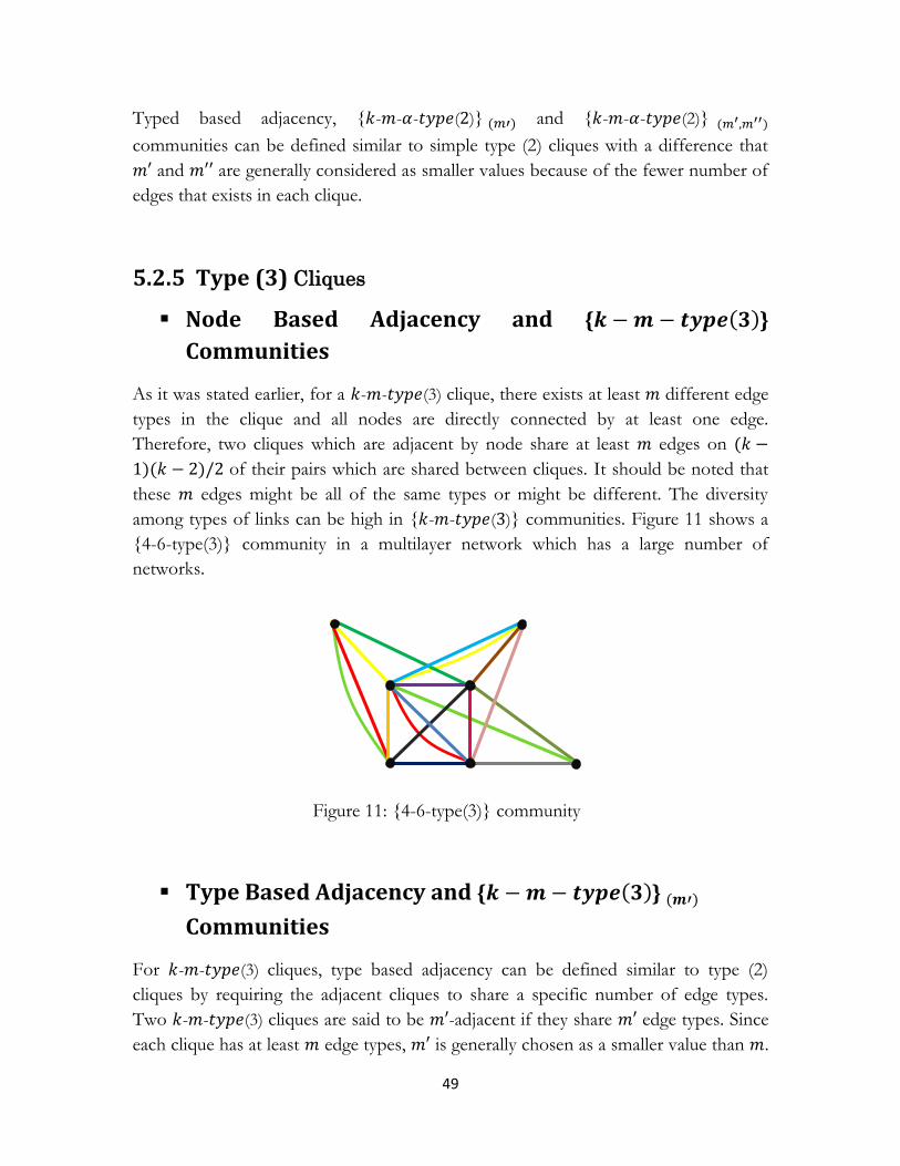
49

Typed based adjacency, - - - ( ) and - - - (2) communities can be defined similar to simple type (2) cliques with a difference that

and are generally considered as smaller values because of the fewer number of edges that exists in each clique.

5.2.5 Type (3) Cliques

Node Based Adjacency and Communities

As it was stated earlier, for a - - (3) clique, there exists at least different edge types in the clique and all nodes are directly connected by at least one edge. Therefore, two cliques which are adjacent by node share at least edges on

of their pairs which are shared between cliques. It should be noted that these edges might be all of the same types or might be different. The diversity among types of links can be high in - - ( ) communities. Figure 11 shows a 4-6-type(3) community in a multilayer network which has a large number of networks.

Type Based Adjacency and Communities

For - - (3) cliques, type based adjacency can be defined similar to type (2) cliques by requiring the adjacent cliques to share a specific number of edge types. Two - - (3) cliques are said to be -adjacent if they share edge types. Since each clique has at least edge types, is generally chosen as a smaller value than .

Figure 11: 4-6-type(3) community

50

Like before, cliques which are not directly connected do not necessarily share any edge types. Figure 12 shows a 3-7-type(3) community. It is worth noting that the number of present networks (colors) is 14 in this figure. This large number makes the distribution of edge types more diverse;; however, some amount of uniformity can be still seen.

( ) Communities

Similar to other types of cliques, it might be of interest to require all cliques which are forming a type (2) community to share some edge types. To achieve this property, similar to - - (2) communities, a - - (3) community is a - - (3) community where all cliques that are forming the community share at least different edge types where . Figure 13 shows a 3-7-type(3) community. It can be seen that two edge types shown by yellow and red are common between all cliques.

Figure 13: 3-7-type(3) community

Figure 12: 3-7-type(3) community

51

5.2.6 Type (3) Quasi Cliques As stated before, a - - - (3) quasi clique includes at least different edge types and part of all of its pairs are directly connected. The discussions and definitions made above for simple type (3) cliques can be generalized to type (3) quasi cliques. The corresponding communities are similar to the ones forming by simple cliques with respect to the distribution of edge types;; however, there is generally less number of edges in the latter case because of the possible existing disconnected nodes. Figure 14(a) shows a 3-4-(1/2)-type(3) community. As can be seen, it has many disconnected nodes and the diversity among types of links is high. Figure 14(b) shows a 3-6-(1/2)-type(3) community.

5.2.7 Type (4) Cliques As defined in previous sections, type(4) cliques should include a specific number of edge types and there is no constraint concerning nodes connectivity. Therefore, type(4) cliques might include many disconnected nodes. For most applications, subgraphs with such characteristics are unlikely to form satisfactory communities. Therefore, the above discussions are not brought here for type (4) cliques.

Figure 14: Type (3) quasi communities

(b) (a)

52

5.3 Comparison between Different Types of Communities

from Theoretical Aspects As it was shown in last sections, there are generally three groups of communities for each specific type of clique;; - - (a) communities, - - (a) communities and - - (a) communities. For the sake of simplicity, these communities are also referred to by their number of subscripts as the number of their parameters. Therefore, these communities have zero, one and two parameters respectively.

According to the definitions, it is quite obvious that a - - (a) community is also a - - (a) community and a - - (a) community is also a - - (a) community. In Section 4.6 it was shown that if is a - - clique, then for it is also a - - clique. This statement can be also generalized to communities with same or less number of parameters. As an example, for , a - - (a) community is also a -

- (b) and consequently a - - (b) community. The complete chain of relations can be shown by a directed graph where different types of communities are denoted by nodes (Figure 15). Since and are supposed to be equal for all communities, for simplicity, the communities are briefly shown by their clique type and the number of their parameters. As an example, - - (1) community is shown by 1 . For two communities like and , can be resulted from if and only if there exists a path from to . As we see, all communities can be derived from the - - (1) community. As we step forward to the right or the bottom, we have communities with less intensity and less sub communities.

Figure 15: Relation between different types of communities

53

If we consider the rows in this graph, in the first row we have communities where there are constraints on the whole cliques forming the community. It means that all cliques should share a specific number of edge types. In the second row we have communities with constraints on adjacent cliques, which means the repetition of edge types is only guaranteed on adjacent cliques and small neighborhoods. In the third row we have communities with no constraints on subgraphs larger than individual cliques. On the other hand, as we step forward from left to right on each row, the constraints on individual cliques are weakened. For quasi communities, we can have a similar graph as Figure 15 by replacing each community by its corresponding quasi community.

5.4 Different Types of Communities in Practice In this section, a discussion is made about the applications of different types of communities. As can be realized from Figure 15, in the case that dense connections in individual networks is required throughout the whole community, - -

(1) communities can be considered as the most relevant communities. As a simple example, consider a 2-layer network where one layer is a physical network, like people living in the same geographical region or working in the same company while the other layer is a social network like Facebook. If the objective is finding individuals who have face-to-face communication in the first layer and are also connected in the second layer, these individuals can form a - - (1) community in the multilayer network.

Recognizing these kinds of communities is computationally more expensive than the other types. Then we have - - (1) and - - (1) communities where the uniformity among types of links is preserved only in small neighborhoods of the size of adjacent cliques or individual cliques. Recognizing these types of communities is less expensive than - - (1) communities. However, they cannot reveal much information about uniformity of types of links throughout the whole community.

On the other hand, we have - - (2) communities where the number of links between nodes is taken into account, but uniformity among types of links is not enforced even on small neighborhoods. This is basically the same approach which is taken in most traditional clustering methods where the multilayer network is

54

converted to a weighted graph. Recognizing these communities is much less expensive that the ones discussed earlier. This approach is mainly taken when uniformity among types of links can be neglected, or when it is required for the communities to have strong connections in all of the networks which are forming the multilayer network, and therefore the multilayer network can be treated as a weighted graph.

As a more constrained kind of type communities, - - (2) communities were defined. In these communities, the multilayer network is treated as a weighted graph respecting individual cliques while some amount of uniformity among edge types is required for larger neighborhoods. However, this uniformity is not enforced throughout the whole community. It can be realized that these types of communities cannot reveal much more information about individual networks than - - (2) communities, and therefore they are less likely of interest. On the other hand, we have - - (1) communities. These kinds of communities could still be a choice when uniformity among types of links is required throughout the community but this constraint is expensive to be enforced on small neighborhoods of size of individual cliques.

As can be realized from above discussions, type and type communities are more or less consistent with the definition of communities in simple networks as it is required that the communities have enough number of links coming from several networks. In contrast, in type communities, a new definition of communities emerges. In this type of communities, a specific number of networks should be present among the connections in each community while there is no strict constraint on the number of internal links. In these communities, rather than having strong connections, we have some interactions between different networks. Therefore, these communities might be of interest when the interaction between different networks is to be taken into account. As an example, it is said that the members of terrorist groups communicate with each other through different networks such that it becomes difficult for these connections to be tracked. These connections might form a type community. Type communities are not discussed with more detail in the thesis and the topic can be considered as a future work of this study.

55

Chapter 6

CPM for Multilayer Networks

6.1 Introduction As it was mentioned in previous chapter, in comparison with other types of communities, - - (1) communities enforce stronger connections in individual networks, and therefore, they are more likely of interest in most applications. In this chapter, a method is proposed for recognizing - -

(1) communities in multilayer networks. The method is a generalization of CPM in simple networks;; however, the complex structure of the multilayer network makes the steps of the method more complex. In the next section, it is briefly explained how CPM works in practice for simple networks. Then in the next sections, a generalizations of the method is proposed for multilayer networks and - - (1) communities.

6.2 Original CPM in Practice As we know, for a given , CPM defines communities as the maximal union of -cliques that can be reached from each other through a series of adjacent -cliques.

56

The corresponding approach in the choice of an appropriate value of has been explained in Section 4.2. In practice, CPM finds these kinds of communities in three main steps: In the first step, the individual maximal cliques are located. Then a matrix called clique-clique overlap matrix is constructed. In the final step, communities are recognized by performing a component analysis of the matrix. The steps of the method are briefly reviewed here. A more detailed explanation of the method can be found in [22].

Locating the Cliques

As it was mentioned before, CPM builds communities from adjacent -cliques;; and therefore, as the first step of the method, the cliques should be located. In a simple network, a maximal clique with more than nodes is trivially a combination of a series of -cliques that can be reached from each other through adjacent -cliques. In addition, two such maximal cliques are part of the same community if they share

nodes. On the other hand, locating maximal cliques is computationally less expensive than individual -cliques. Therefore, the proposed approach in [22] locates maximal cliques rather than individual -cliques. The largest possible clique size in the network is determined from the degree-sequence of the corresponding graph;; the non-increasing sequence of the vertex degrees. To find all maximal cliques, the authors propose an algorithm which starts with the largest possible clique size, repeatedly chooses a node and finds every clique of this size including that node, then deletes the node and its edges. When no nodes are left, the clique size is decreased by one and the algorithm is restarted on the original graph. It should be noted that the cliques which have been already found influence the procedure of finding other cliques as the unrevealed smaller cliques cannot be subsets of them. To find all cliques of a specific size like and including a specific node like , the algorithm starts with two sets of nodes like and where initially contains only and contains all of the neighbors of . The cliques that include are trivially formed by and the possible combinations of its neighbor. In each iteration of the algorithm, one node like is transferred from to , and then those nodes in which are not connected to are removed from . This procedure continues until becomes of the size . If becomes empty before reaches size , or if the union of the sets and can be included in an already found larger clique, the current iteration of the algorithm is skipped and other possible combinations are tried.

57

Clique-­‐‑Clique Overlap Matrix

After locating maximal cliques, a matrix which is called the clique-clique overlap matrix is constructed. Suppose that is a set containing different sets of vertices like

where each contains the nodes of a maximal clique. The elements in are sorted in descending order of . Without loss of generality, suppose that has elements and the th element in is . Now for a given , the clique-clique overlap matrix is constructed in two steps as follows: In first step, each diagonal entry of the matrix, , is equal to the size of and each off-diagonal entry of the matrix,

, is the number of common vertices in and . In the second step, first each diagonal entry smaller than and each off-diagonal entry smaller than is replaced by zero. Then any none zero entry of the matrix is replaced by 1. This procedure gives us a symmetric matrix where each non-zero diagonal entry like corresponds to a maximal clique like with at least nodes, and each non-zero off-diagonal entry of the matrix like shows that and share at least common nodes and therefore they are adjacent.

From Clique-­‐‑Clique Overlap Matrix to Communities

In a simple network, each individual clique and all of its adjacent cliques can be included in exactly one community. This general rule is the key to detect communities from the clique-clique overlap matrix. Community detection is started with . First, all adjacent cliques to are recognized from the first row (or the first column) of the matrix. Then for each adjacent clique to like , all adjacent cliques to are recognized from the th row. This procedure continues for all cliques until no more adjacent clique can be found. The union of these cliques forms the first community. For the second community, we start with the first clique that is not included in the first community and its corresponding diagonal entry in the matrix is non-zero. This procedure continues until no clique is left, and therefore no new community can be found.

6.3 CPM for Multilayer Networks In this section, a generalization of CPM is proposed for multilayer networks and - - (1) communities. As it was mentioned before, a - -

(1) community is a community forming by maximal union of - -

58

(1) cliques that can be reached from each other through a series of -adjacent - - (1) cliques and the cliques forming the community share at least edge

types throughout the whole community on all of their pairs. The objective of this chapter is to propose a method to find such communities. The method finds communities in three steps: The first is locating - - (1) cliques, then recognizing

-adjacent cliques between cliques found in the first step, and then the final step is finding - - (1) communities. It should be noted that the method is not dependent on the values of and , therefore, for the sake of simplicity, it is supposed that .

6.3.1 Locating the Cliques In Section 6.2, it was shown that in a simple network, maximal cliques and -cliques can be interchangeably used in CPM while searching for maximal cliques is practically more efficient. In multilayer networks, however, this interchangeability is not trivial as before and it should be obtained under more sophisticated conditions. On the other hand, - - (1) cliques in multilayer networks generally appear with less frequency than -cliques in single networks. Therefore, the proposed method in the thesis locates - - (1) cliques rather than maximal cliques.

Similar to original CPM, to find all - -type(1) cliques in the network, we find all --type(1) cliques containing each individual node, then we remove that node and

continue with another node in the reduced network. As it was defined in Section 4.4, for each two nodes like and , denotes the set of all existing edge types(labels) between and . Also for a given subset of like , is the set of all common edge types between all pairs of nodes in , or in other words, . In addition, for two disjoint subsets of like and and a node in like , is defined as the common edge types between all pairs of nodes including and a node in ;; in other words, .

The -­‐‑ -­‐‑ Cliques Finding Algorithm

To find all - -type(1) cliques in the network including a specific node like , a recursive function called is proposed (Algorithm 1). The function starts with two sets of nodes like and where initially contains only , and contains all -neighbors of ;; the nodes that are connected to on at least networks. The

59

objective is transferring different combinations of nodes from to such that the corresponding resulted subgraphs would be - -type(1) cliques. As can be seen in the lines 4 and 5 of the algorithm, at each iteration one node is transferred from to . If the current clique has the acceptable size, a new iteration is started (lines 6, 7 and 8), otherwise, more acceptable nodes are recognized in line 9, then is run again to try more combinations of nodes of the new set. It should be noted that, considering and , if a node can be added to the current set , it can not necessarily be added to if more nodes are added to it even if is not still of size . Therefore, all possible combinations of nodes should be taken into account. After finding all cliques, returns a set like which includes different sets of nodes, each set corresponds to a - -type(1) clique.

ALGORITHM 1

1.

2.

3.

4. ;;

5. ;;

6. :

7. ;;

8. ;;

9.

10. ;;

11.

Now to find all cliques in the network, we can apply to each individual node, then remove the node from the network and continue with another node. For a multilayer network like , suppose that is a given subset of the set of all vertices in . For each in , is the set of all -neighbors of in ;; the nodes in that are directly connected to on at least networks. The function

60

is proposed here to find all possible - - (1) cliques in the multilayer network (Algorithm 2).

ALGORITHM 2

1. :

2. ;

3. ;

4.

5.

6.

7. ;

8. ;

9. ;

10.

6.3.2 Adjacent Cliques and Clique-­‐‑Clique Adjacency Matrix As it was mentioned in Section 6.2, in a simple network, each clique can be included in exactly one community. However, this statement is not necessarily true for - -type(1) cliques in multilayer networks as a - -type(1) clique can be -adjacent to several different - -type(1) cliques on different sets of edge types of size at least while the intersection of these sets has a smaller size than , and therefore they cannot be included in the same communities. It can be realized that detecting communities in multilayer networks is not as straightforward as simple networks as each clique can be included in different communities with different combinations of its adjacent cliques. As a result, the clique-clique overlap matrix defined for original CPM cannot be used directly for community detection in multilayer networks. The proposed method in the thesis recommends constructing an adjacency matrix rather than overlap matrix. The matrix is referred to as clique-clique adjacency matrix.

Suppose that is the set of all - -type(1) cliques in a multilayer network like . In other words, contains different sets of nodes like where the nodes in each set

61

corresponds to a unique - -type(1) clique in . For each two cliques like and , let be the number of common vertices between the two cliques. Also suppose is the Kronecker delta which returns 1 if and share at least common edge types on all of their pairs, otherwise zero. In other words, returns 1 if and only if

. As it was mentioned in previous chapters, two - -type(1) cliques are -adjacent if they share nodes and they share at least common edge types on all of their pairs. Therefore, for two -adjacent - -type(1) cliques we have

. Suppose that the set has elements. The clique-clique adjacency matrix is constructed as follows: each diagonal entry of the matrix, , is equal to zero. Each off-diagonal entry of the matrix, , is equal to 1 if is equal to , otherwise zero. This gives us the adjacency matrix of the cliques. So two cliques like and are -adjacent if and only if . For the set of all cliques , the clique-clique adjacency matrix can be obtained by function defined as follows:

ALGORITHM 3

1. :

2.

3.

4. :

5. ;;

6.

7. :

8.

9.

10. ;;

11.

62

Now for each specific clique like in the set of cliques , its neighbors can be recognized from the clique-clique adjacency matrix . The function is defined to return neighbors of each clique as follows:

ALGORITHM 4

Figure 16 shows a multilayer network and all of its 3-3-type(1) cliques. Suppose that targets are - - (1) communities. The adjacency matrix of 3-adjacenct cliques can be seen in Figure 17.

Figure 16: 3-3-type(1) cliques in a multilayer network

63

6.3.3 From Adjacent Cliques to Communities The objective of this section is to propose a method for recovering communities form clique-clique adjacency matrix. As mentioned in previous section, each clique can be included in different communities with different combinations of its adjacent cliques. On the other hand, as it was shown in Section 5.2.1, -adjacency of pairs of cliques does not guarantee the repetition of same edge types for cliques that are not directly adjacent. Therefore, the adjacency matrix cannot be directly used to recognize communities.

The clique-clique adjacency matrix corresponds to the adjacency matrix of a graph where nodes represent cliques. For a multilayer network like , suppose that is the corresponding clique-clique adjacency graph where the vertex in represents the clique . In this graph, each two nodes are directly connected if the corresponding cliques are -adjacent. In addition, two cliques can be reached from each other through -adjacent cliques if there exists a path between the corresponding nodes in the graph. It should be reminded that this does not still guarantee the repetition of same edge types. Figure 18(a) shows the clique-clique adjacency graph of the adjacency matrix in Figure 17. It should be noted that for this simple example of multilayer networks, the clique-clique adjacency graph does not include any cycle;; however, in general, such graphs can include cycles as well. In this example, and

0 1 0 0 0 0 0 0 0 0 1 0 0 0 0 0 0 0 1 0 0 0 0 0 0 0 0 0 0 0 0 0 0 0 1 0 0 0 0 0 0 0 0 1 0 0 0 0 0 0 0 0 0 0 0 0 1 0 0 0 0 0 0 0 0 1 0 1 0 0 0 0 0 0 0 0 1 0 1 0 0 1 0 0 0 0 0 1 0 1 0 0 0 0 0 0 0 0 1 0

Figure 17: clique-clique adjacency matrix

64

can be reached from each other through a path, however, as can be seen in Figure 16, and cannot be included in the same - - (1) community.

As it was mentioned earlier, for a - - (1) clique like , is the set of all edge types which are repeated on all pairs in . Now for each vertex like in , we associate the set to that vertex. Considering this notation, two cliques can be reached from each other through -adjacent cliques with the constraint that all cliques share at least edge types on all of their pairs if and only if there is a path between the corresponding nodes in the graph where the intersection of the associated sets to the nodes of the path has at least elements. Suppose that

is an ordered set corresponds to the nodes in the path from to in Figure 18(a). It can be easily seen that the above constraint holds for these nodes and the corresponding cliques for equal to 3. In addition, if is added to the mentioned set, this constraint still holds but no other node than can be added without violating our constraint. On the other hand, this set is not the only set which can contain as the set also fulfills the constraint. It can be realized that each community corresponds to the nodes of a maximal tree in the clique-clique adjacency graph where the intersection of the associated sets to all nodes has at least

elements. Figure 18(b) shows all of such trees in our example. In the following, a method is proposed to find the nodes of the mentioned maximal trees.

To find nodes of all maximal trees with the mentioned constraint, we find nodes of all maximal trees including each individual node with same constraint, then we delete

Figure 18: clique-clique adjacency graph and maximal trees

(a) (b)

65

that node from the graph and continue with another node. The resulted sets of nodes might be subsets of the sets found in previous iterations;; therefore, redundant sets should be ignored. As we know, for each two directly connected vertices like and

we have , therefore each two connected nodes corresponds to a sub-community of at least one community. For each specific node in the graph like

, the method starts with a set initially containing only , and a set containing all the neighbors of . At the first iteration, one node like is transferred from to and then we add all those neighbors of which are not in to the set . Therefore

contains all neighbors of the nodes in except the ones which are in . We also define as the intersection of associated sets to the nodes in which is

at this step. The objective is to enlarge by the neighbors of its nodes such that the tree constraint is still hold. So we transfer one candidate node like from to such that . Then and are updated like before. This procedure continues until no node can be added to . Then other possible combinations of nodes are tried. It should be noted that in a regular tree, if a node can be added to the current tree, it can be also added to the tree after adding other nodes to it. But in our special tree, this statement is not necessarily true. As an example, starting from , both and can be added to in the mentioned example in Figure 18(a) to form - - (1) communities;; however none of these cliques can be added to this set after the other. Therefore, all combinations of nodes should be taken into account.

In the above, the procedure was explained for a modeled graph. Now in the following, a function called is introduced to find all sets of adjacent cliques forming a maximal tree in our graph model that include a specific clique (Algorithm 5). takes four inputs: the first input is a set like containing the main clique like which corresponds to a node in our modeled graph, the second input is a set containing all adjacent cliques to which are the neighbors of the nodes in the graph, the third input is the set of all cliques and the fourth input is the corresponding adjacency matrix (line 2 in the algorithm). As can be seen in line 4, in each iteration one clique from the set of neighbors is added to the set of adjacent cliques. After adding each clique, in line 5, the set of neighbors is updated by adding the neighbors of the clique recently added. Then other possible acceptable cliques are recognized from the neighbors in line 6. If the set of acceptable neighbors becomes empty, the current set of adjacent cliques is added to the set of trees, , and a new iteration is started (lines 7, 8 and 9). If there are still acceptable neighbors, is run again to try other possible combinations. The function returns the set

66

containing different sets of cliques including where the cliques in each set form a specific community.

ALGORITHM 5

1.

2. :

3.

4.

5.

6.

7. :

8. ;

9. ;

10. ;

11.

Now to find all communities, should be applied to all the cliques found in the first step. For each clique like in the set of cliques , we find all communities including then we remove from and we continue with another clique. This can be performed by the following function in Algorithm 6. The function takes the set of cliques as input. It calls to compute the corresponding adjacency matrix. In each iteration, the set of adjacent cliques containing one specific clique are recognized by calling (lines 3 to 6). As it was mentioned before, this approach might result in sub-communities of the communities found in previous iterations. In line 7 and 8, those sets that are not the subsets of the sets previously found are recognized and added to the set of communities. It should be noted that this task can be done more efficiently in the time of implementation by comparing the edge types. At the end of each iteration, the clique is removed from the set of cliques (line 9) and its corresponding row and column in the adjacency matrix is deleted (line 10).

67

ALGORITHM 6

1. :

2. ;;

3.

4.

5.

6. ;;

7.

8.

9.

10.

11. ;;

6.4 Conclusion The overall purpose of this study was to discuss how CPM can be used to find communities in multilayer networks. It has been shown that cliques which are the components of communities can be defined in different ways where each specific definition results in communities with a specific structure. In the definition of cliques and communities, three main approaches were taken into account. In the first approach, it is expected that the participants of a community in a multilayer network are densely connected in single networks. The second approach is a more flexible form of the first approach where it is necessary for the participants of the communities to be densely connected in the multilayer network while less strict constraints are enforced on their connections in single networks. In the third approach, the strength of the communities is evaluated by the number of contributing networks while the density of the connections is not taken into account. These three approaches were resulted in three types of communities;; type(1), type(2) and type(3) communities respectively.

68

After defining the communities precisely, a discussion was made about their relation from both theoretical and practical aspects. It has been shown that there is a hierarchy in the definitions of communities and as we go from type(1) communities to type(3) communities, the enforced constraints are weakened. It was also shown that uncovering type(1) communities is practically more expensive than other types of communities.

In the last part of the thesis, an algorithm was proposed to uncover type(1) communities with their most strict constraints where it is required for all nodes in the community to be densely connected on a specific number of networks. The algorithm can find communities across the layers, and it is claimed to be complete. Although these properties cause the algorithm to appear computationally expensive, it is believed to be effective for real networks as the strict constraints enforcing by the algorithm decrease the number of iterations significantly.

6.3.3 Future Work For future work, the method is a topic for improvement. The proposed algorithms have a recursive behavior because the problem is finding all possible communities across the layers. It would be interesting to enhance the method such that it can still find all possible solutions while the efficiency of the method is improved. It would be also interesting to improve the method such that it can uncover communities by locating maximal cliques. Implementation of the algorithm on dense real networks can give a better understanding of its efficiency. Another possible evaluation is comparing the efficiency of the method with the original CPM on real examples.

Another problem which is not addressed in the thesis is the relation between communities which are recognized by our proposed method in multilayer networks and the ones that the original CPM finds in the related single networks. Can the method find communities that are not visible in individual layers? What would happen to the communities when we change the number of contributing layers? These questions can be addressed in further research.

69

Appendix A

An Introduction to Graph theory

A.1 Simple Graphs

A is a representation model of a set of objects and their relations. In a graph, each object is represented by a or , and the relations between objects are represented by or . A graph like is denoted by where and are the set of vertices and edges in respectively. Two vertices in are said to be

if an edge exists between them. A is a graph where each edge in the graph is directed from one vertex to another. A is an undirected graph where there exists at most one edge between each two vertices in the graph and the graph does not contain any . A loop is an edge which connects a vertex to itself. A is a graph where a weight (label) is associated with each edge in the graph.

A.2 Subgraphs

For a graph like , is said to be a of if the sets of vertices and edges in are subsets of the sets of vertices and edges in ;; in other words, and

. A subgraph of a graph is said to be an if each two vertices in which are connected in are also connected in .

70

A.3 Vertex Degree

The of a vertex of a graph is the number of edges incident on that vertex. The degree of a node like is denoted by . For a graph like , the

of is a diagonal matrix where each diagonal entry is equal to the degree of a vertex in the graph.

A.4 Paths, Walks and Cycles

A is a sequence of edges that connect a sequence of distinct vertices. The between two vertices is the number of edges (sum of weights) in the

shortest path between two vertices. If no path exists between two vertices, the vertices are said to have a distance of infinity. The of a graph is the greatest distance between any pair of vertices in the graph. A is a sequence of alternating vertices and edges, beginning and ending with vertices, where each edge's endpoints are the preceding and following vertices in the sequence. A or is a walk which starts and ends with the same vertex.

A.5 Connectivity

A graph is said to be if there exists at least one path between each two vertices in the graph;; otherwise, the graph is called . A of a graph is a subgraph where there exists at least one path between each two vertices in the subgraph while all vertices in the subgraph are disconnected to the rest of the graph. In other words, each component is a maximal connected subgraph of the graph.

A.6 Trees

A is a simple connected graph with no cycle. There exists exactly one path between each two vertices in a tree. A tree with more than one vertex has at least two vertices of degree one. A vertex of degree one is called a .

A.7 Adjacency Matrix

is a square matrix which represents a graph. Each element in the adjacency matrix corresponds to the connection of a pair of vertices. For an unweighted simple graph, adjacency matrix is a symmetric matrix with entries of zero or 1. Each diagonal entry of this matrix is zero and each off-diagonal entry of the

71

matrix is equal to one if and only if the corresponding vertices are adjacent. For a weighted graph, the elements in the adjacency matrix are the corresponding weights.

A.8 Multigraphs

A is a graph where the multiple edges and loops are permitted. In other words, in a multigraph, two nodes can be connected by more than one edge, and a node can be connected to itself.

72

Bibliography

[1] S. Fortunato, Community Detection in Graph, Physics Reports, vol. 486, pp. 75-174 (2010)

[2] R.D. Alba, A Graph Theoretic Definition of a Sociometric Clique. Journal of Mathematical Sociology 3: (1973) 113-126.

[3] R.J. Mokken, Cliques, Clubs and Clans, Qual. Quant. 13 (1979) 161 173.

[4] S.B. Seidman and B.L. Foster, A Graph-Theoretic Generalization of the Clique Concept. Journal of Mathematical Sociology. 6, 139-154 (1978)

[5] S.B. Seidman, Network Structure and Minimum Degree. Social Networks. 5, 269-287 (1983)

[6] H. Matsuda, T. Ishihara, and A. Hashimoto, Classifying Molecular Sequences Using a Linkage Graph with Their Pairwise Similarities, Theor. Comput. Sci., 210:305 325, 1999.

[7] F. Radicchi, C. Castellano, F. Cecconi, V. Loreto, and D. Parisi, Defining and identifying communities in networks. Proc. Natl. Acad. Sci. USA 101, 2658 2663 (2004).

[8] Y. Hu, H. Chen, P. Zhang, M. Li, Z. Di and Y. Fan (2008) Comparative Definition of Community and Corresponding Identifying Algorithm. Phys Rev E 78: 026121.

[9] S.P. Borgatti, M.G. Everett and P. Shirey, 1990. LS sets, lambda sets and other cohesive subsets. Social Networks, 12: 337-357.

[10] R.S. Burt, 1976, Positions in networks, Social Forces 55, 93-122.

[11] S. Wasserman, K. Faust, 1994. Social Network Analysis: Methods and Applications. Cambridge: Cambridge University Press.

73

[12] M. E. J. Newman, M. Girvan, Finding and Evaluating Community Structure in Networks. Phys. Rev. E 69, 026113 (2004).

[13] B. W. Kernighan, S. Lin, An Efficient Heuristic Procedure for Partitioning Graphs, Bell System Tech. Journal 49 (1970), pp. 291-307.

[14] F. Chung, 1997. Spectral Graph Theory, Number 92 in CBMS Regional Conference Series in Mathematics (American Mathematical Society, Providence, USA).

[15] M. Fiedler, Algebraic Connectivity of Graphs, Czechoslovak Mathematical Journal: 23 (98), 1973.

[16] M. Fiedler, Laplacian of Graphs and Algebraic Connectivity, Combinatorics and Graph Theory 25:57-70, 1989.

[17] B. Mohar, The Laplacian Spectrum of Graphs, in Graph Theory, Combinatorics, and Applications, Vol. 2, Ed. Y. Alavi, G. Chartrand, O.R. Oellermann, A.J. Schwenk, Wiley, 1991, pp. 871 898.

[18] A. Pothen, 1997, Graph Partitioning Algorithms with Applications to Scientific Computing, Technical Report, Norfolk, VA, USA.

[19] J. B. MacQueen, 1967, in Proc. of the fifth Berkeley Symposium on Mathematical Statistics and Probability, edited by L. M. L. Cam and J. Neyman (University of California Press, Berkeley, USA), volume 1, pp. 281-297.

[20] M. Girvan and M. E. J. Newman, Community structure in social and biological networks. Proc. Natl. Acad. Sci. USA 99, 7821 7826 (2002).

[21] M. E. J. Newman, Fast Algorithm for Detecting Community Structure in Networks. Phys. Rev. E 69, 066133 (2004).

[22] G. Palla, I. Derényi, I. Farkas, T. Vicsek, Uncovering the Overlapping Community Structure of Complex Networks in Nature and Society. Nature 435, 814818 (2005)

[23] T. Nepusz, A. Petroczi, L. Negyessy, and F. Bazso, 2008. Fuzzy Communities and the Concept of Bridgeness in Complex Networks. Phys. Rev. E 77, 1.

[24] D. Cai, Z. Shao, X. He, X. Yan, J. Han, Community Mining From Multi-relational networks. In: Jorge, A.M., Torgo, L., Brazdil, P.B., Camacho, R., Gama, J.

74

(eds.) PKDD 2005. LNCS (LNAI), vol. 3721, pp. 445 452. Springer, Heidelberg (2005)

[25] M. Rodriguez, J. Shinavier, Exposing Multi-Relational Networks to Single-Relational Network Analysis Algorithms. Journal of Informetrics 4(1), 29 41 (2010).

[26] L. Tang, X. Wang, H. Liu, Community Detection via Heterogeneous Interaction Analysis. Data Mining Knowledge Discovery 25(1), 1 33 (2012).

[27] Z. Wu, W. Yin, J. Cao, G. Xu, A. Cuzzocrea (2013) Community Detection in Multi-Relational Social Networks. WISE 8181:43 56.

[28] W. Tang, Z. Lu, and I. Dhillon, Clustering with Multiple Graphs, in International Conference on Data Mining, Miami, Florida, USA, Dec 2009.

[29] A. Kumar, P. Rai, and H. Daum´e III, Co-regularized Spectral Clustering with Multiple Kernels, NIPS 2010 Workshop: New Directions in Multiple Kernel Learning, 2010.

[30] X. Dong, P. Frossard, P. Vandergheynst, and N. Nefedov, Clustering with Multi-Layer Graphs: A Spectral Perspective, IEEE Transactions on Signal Processing, vol. 60, no. 11, pp. 5820 5831, Nov 2012.

[31] P. J. Mucha, T. Richardson, K. Macon, M. A. Porter, and J. P. Onnela, Community Structure in Time-Dependent, Multiscale, and Multiplex Networks, Science 328 (2010) 876-878.

[32] X. Liu, W. Liu, T. Murata, K. Wakita, A Framework for Community Detection in Heterogeneous Multi-Relational Networks, Advances in Complex Systems 17(6) (2014)

[33] T. Murata, T. Ikeya, A New Modularity for Detecting One-to-many Correspondence of Communities in Bipartite Networks, Advances in Complex Systems 13 (2010) 19-31.

[34] T. Murata, Detecting Communities from Tripartite Networks, in Proceedings of the 19th International Conference on World Wide Web (Raleigh, NC, USA, 2010), pp. 1159-1160.

[35] A. Sole-Ribalta, M. De Domenico, S. Gómez, and A. Arenas, Centrality Rankings in Multiplex Networks, in ACM conference on Web science - WebSci. New York, New York, USA: ACM Press, Jun. 2014, pp. 149 155.

75

[36] B. Boden, S. Gunnemann, H. Hoffmann, and T. Seidl, Mining Coherent Subgraphs in Multi-Layer Graphs with Edge Labels, in SIGKDD, pages 1258 1266 (2012).

[37] andom Graphs, I. Publicationes Mathematicae (Debrecen), 6:290-297, 1959.

[38] I. Der´enyi, G. Palla, and T. Vicsek, Clique Percolation in Random Networks, 2005, Phys. Rev. Lett. 94(16), 160202.

[39] J. P. Onnela, J. Saramäki, J. Kertész and K. Kaski, Intensity and Coherence of Motifs in Weighted Complex Networks, 2005 Phys. Rev. E 71 065103.

[40] I. J. Farkas, D. Ab´el, G. Palla and T. Vicsek, Weighted Network Modules, New Journal of Physics, 9 (2007), 180.

[41] S. Lloyd, (1982), Least Squares Quantization in PCM, IEEE Transactions on Information Theory 28 (2): 129 137