NAVAL POSTGRADUATE SCHOOLFigure 24. ANSYS Explicit Dynamic refined mesh and support constraints for...

NAVAL POSTGRADUATE

SCHOOL

MONTEREY, CALIFORNIA

THESIS

Approved for public release; distribution is unlimited

COMPOSITE CASE DEVELOPMENT FOR WEAPONS APPLICATIONS AND TESTING

by

Cassandra C. Mitchell

March 2015

Thesis Advisor: Young W. Kwon Co-Advisor: John D. Molitoris

THIS PAGE INTENTIONALLY LEFT BLANK

REPORT DOCUMENTATION PAGE Form Approved OMB No. 0704-0188 Public reporting burden for this collection of information is estimated to average 1 hour per response, including the time for reviewing instruction, searching existing data sources, gathering and maintaining the data needed, and completing and reviewing the collection of information. Send comments regarding this burden estimate or any other aspect of this collection of information, including suggestions for reducing this burden, to Washington headquarters Services, Directorate for Information Operations and Reports, 1215 Jefferson Davis Highway, Suite 1204, Arlington, VA 22202-4302, and to the Office of Management and Budget, Paperwork Reduction Proiect (0704-0188) Washinoton DC 20503. 1. AGENCY USE ONLY (Leave blank) 1 2. REPORT DATE I 3. REPORT TYPE AND DATES COVERED

March 2015 Master's Thesis

4. TITLE AND SUBTITLE 5. FUNDING NUMBERS COMPOSITE CASE DEVELOPMENT FOR WEAPONS APPLICATIONS AND TESTING 6. AUTHOR(S) Cassandra C. Mitchell

7. PERFORMING ORGANIZATION NAME(S) AND ADDRESS(ES) 8. PERFORMING ORGANIZATION Naval Postgraduate School REPORT NUMBER Monterev. CA 93943-5000

9. SPONSORING /MONITORING AGENCY NAME(S) AND ADDRESS(ES) 10. SPONSORING/MONITORING Lawrence Livermore National Laboratory AGENCY REPORT NUMBER

11 . SUPPLEMENTARY NOTES The views expressed in this thesis are those of the author and do not reflect the official policy or position of the Department of Defense or the U.S. Government.

12a. DISTRIBUTION I AVAILABILITY STATEMENT 12b. DISTRIBUTION CODE Approved for public release; distribution is unlimited

13. ABSTRACT (maximum 200 words)

Analys is of the dynamic response of cylindrical carbon fiber/epoxy cases contain ing high explosive fill was conducted using ALE3D finite e lement software. To develop an accurate model, material compression testing was performed with a Split Hopkinson Pressure Bar apparatus and lnstron SATEC machine to verify high-strain rate and low-strain rate behavior, respectively. Resulting failure modes of compression test samples were similar to those found in current literature. lzod pendulum impact testing was performed to provide an intermediate strain rate comparison. An ANSYS model w as developed to ensure fracture energy values obtained from lzod impact testing resulted in material stresses w ithin the bounds of the high strain rate and low strain rate testing. The result ing materia l properties were input parameters for the ALE3D carbon fiber composite model developed by Kwon. The carbon fiber model and this thesis research provide critical information for testing and development in support of Lawrence Livermore National Laboratory's Agent Defeat Penetrator Project.

14. SUBJECT TERMS Carbon fiber epoxy, carbon fiber composite, ALE3D, Split Hopkinson 15. NUMBER OF Pressure Bar, compression testing, lzod impact testing, Agent Defeat Penetrator PAGES

17. SECURITY 18. SECURITY CLASSIFICATION OF CLASSIFICATION OF THIS REPORT PAGE

Unclassified Unclassified NSN 754~1-280-5500

119 16. PRICE CODE

19. SECURITY 20. LIMITATION OF CLASSIFICATION OF ABSTRACT ABSTRACT

Unclassified uu Standard Form 298 (Rev. 2-89) Prescribed by ANSI Std. 239-18

ii


iii

Approved for public release; distribution is unlimited

COMPOSITE CASE DEVELOPMENT FOR WEAPONS APPLICATIONS AND TESTING

Cassandra C. Mitchell Lieutenant, United States Navy

B.S., Alfred University, 2007

Submitted in partial fulfillment of the requirements for the degree of

MASTER OF SCIENCE IN MECHANICAL ENGINEERING

from the

NAVAL POSTGRADUATE SCHOOL March 2015

Author: Cassandra C. Mitchell

Approved by: Young W. Kwon Thesis Advisor

John D. Molitoris, Lawrence Livermore National Laboratory Co-Advisor

Garth V. Hobson Chair, Department of Mechanical & Aerospace Engineering

iv


v

ABSTRACT

Analysis of the dynamic response of cylindrical carbon fiber/epoxy cases

containing high explosive fill was conducted using ALE3D finite element

software. To develop an accurate model, material compression testing was

performed with a Split Hopkinson Pressure Bar apparatus and Instron SATEC

machine to verify high-strain rate and low-strain rate behavior, respectively.

Resulting failure modes of compression test samples were similar to those found

in current literature. Izod pendulum impact testing was performed to provide an

intermediate strain rate comparison. An ANSYS model was developed to ensure

fracture energy values obtained from Izod impact testing resulted in material

stresses within the bounds of the high strain rate and low strain rate testing. The

resulting material properties were input parameters for the ALE3D carbon fiber

composite model developed by Kwon. The carbon fiber model and this thesis

research provide critical information for testing and development in support of

Lawrence Livermore National Laboratory’s Agent Defeat Penetrator Project.

vi


vii

TABLE OF CONTENTS

I. INTRODUCTION ............................................................................................. 1 A. BACKGROUND ................................................................................... 1 B. THESIS OBJECTIVE ........................................................................... 5 C. EXPERIMENTAL OVERVIEW ............................................................. 6 D. LITERATURE REVIEW ........................................................................ 9

II. QUASI-STATIC AND DYNAMIC COMPRESSION TESTING ...................... 11 A. QUASI-STATIC COMPRESSION TESTING BACKGROUND .......... 11 B. QUASI-STATIC COMPRESSION TESTING PROCEDURE .............. 11 C. INSTRON COMPRESSION TEST RESULTS .................................... 13 D. DYNAMIC COMPRESSION TESTING BACKGROUND ................... 17 E. SHPB SAMPLE PREPARATION AND TESTING ............................. 18 F. SHPB RESULTS ................................................................................ 19

III. IZOD EXPERIMENTAL IMPACT TESTING ................................................. 27 A. IZOD TESTING BACKGROUND ....................................................... 27 B. IZOD TESTING PROCEDURE .......................................................... 28 C. ACRYLIC IZOD IMPACT RESULTS .................................................. 29 D. KAFB CASE 1 IMPACT RESULTS ................................................... 30 E. LLNL CASE 2 IMPACT RESULTS .................................................... 33

IV. IZOD MODELING WITH ANSYS EXPLICIT DYNAMICS ............................. 35 A. BACKGROUND ................................................................................. 35 B. PROBLEM SET-UP ........................................................................... 35 C. IZOD IMPACT MODEL RESULTS ..................................................... 37

V. ALE3D HIGH-EXPLOSIVE FILLED CASE MODEL ..................................... 41 A. MODEL BACKGROUND ................................................................... 41 B. IMPLEMENTATION OF THE CARBON FIBER MODEL ................... 46 C. COMPARISON OF STEEL CASE AND CFC CASE ......................... 48 D. ALE3D MODEL CONCLUSIONS ...................................................... 69

VI. CONCLUSIONS ............................................................................................ 71 A. EXPERIMENTAL TESTING REMARKS ............................................ 71 B. ALE3D MODELING REMARKS ........................................................ 72 C. RECOMMENDED FUTURE WORK ................................................... 73

APPENDIX A. CALCULATIONS FOR CONTROL SAMPLE (HY-80 STEEL) TO DETERMINE TEST MACHINE COMPLIANCE ............................................ 75

APPENDIX B. ADDITIONAL EXPERIMENTAL RESULTS .................................... 79 A. LLNL CASE 2 “SCRAP” SAMPLE RESULTS .................................. 79

APPENDIX C. ADDITIONAL ALE3D CODE ........................................................... 81 A. CFC CODE AND NOTES ................................................................... 81 B. CFC ALE3D INPUT CODE ................................................................ 85

viii

LIST OF REFERENCES .......................................................................................... 95

INITIAL DISTRIBUTION LIST ................................................................................. 99

ix

LIST OF FIGURES

Figure 1. Artist’s concept of the Agent Defeat Penetrator, from [4]. ..................... 2 Figure 2. Conceptual flexible agent defeat weapon designed with high-

strength carbon fiber composite case, from [4]. .................................... 3 Figure 3. Schematic of high-strength carbon fiber detonation test article

utilized in support of the ADP project, from [4]. .................................... 4 Figure 4. Experimental testing at Lawrence Livermore National Laboratory

Energetic Materials Center of acrylic (left) and carbon fiber composite (right) cases containing high explosive payload, from [4]. ... 5

Figure 5. Samples extracted from the acrylic cylindrical case. ............................ 7 Figure 6. Samples extracted from KAFB CFC case 1. ........................................ 7 Figure 7. Images demonstrating LLNL case 2 and typical dimensions of

Carbon Fiber/Epoxy Cases wound at LLNL. ........................................ 8 Figure 8. KAFB CFC case data for three quasi-static compression test

orientations. ........................................................................................ 12 Figure 9. LLNL case 2 data for three quasi-static compression test

orientations. ........................................................................................ 13 Figure 10. Image of failed samples from KAFB case 1 subjected to radial,

circumferential and axial compression orientations. ........................... 14 Figure 11. Image of failed samples from LLNL case 2 subjected to radial,

circumferential and axial compression orientations. ........................... 14 Figure 12. Out-of-plane (radial) (left) and in-plane (circumferential) (right)

quasi-static compression of Ma et al.’s woven fabric carbon fiber composite sample, after [6]. ............................................................... 14

Figure 13. Schematic of Split Hopkinson Pressure Bar apparatus, after [6]. ....... 18 Figure 14. Raw Hopkinson data collected for carbon fiber LLNL case sample

2. ........................................................................................................ 19 Figure 15. SHPB stress-strain data for the acrylic samples subject to varying

gas gun pressures. ............................................................................. 20 Figure 16. SHPB stress-strain data for the CFC samples subject to constant

gas gun pressure of 50psi. ................................................................. 23 Figure 17. Fractured sample (LLNL sample 2: circumferential orientation)

depicting delamination and failure. ..................................................... 23 Figure 18. Fractured sample (LLNL sample 1: radial orientation) depicting

shear damage and failure. .................................................................. 24 Figure 19. Out-of-plane (radial) (left) and in-plane (circumferential) (right) high

strain rate compression of Ma et al.’s woven fabric carbon fiber composite sample, after [6]. ............................................................... 25

Figure 20. Tinius Olsen low energy impact system for plastics, from [23]. .......... 28 Figure 21. Photo of acrylic samples following impact. Half of sample 5 was lost

due to the force of the strike. .............................................................. 30 Figure 22. Image of KAFB case samples following impact testing. ..................... 31 Figure 23. Image of LLNL case 2 samples following impact testing. ................... 33

x

Figure 24. ANSYS Explicit Dynamic refined mesh and support constraints for Izod pendulum impact problem. Plane of interest is outlined immediately above the supports. ........................................................ 36

Figure 25. Von-Mises Stress along the plane of the Izod hammer impact for the Aluminum 6061 test specimen. .................................................... 38

Figure 26. Von Mises stress of CFC Izod sample subject to radial strike orientation (impact wedge not shown). ............................................... 39

Figure 27. Von Mises stress associated with the circumferential strike orientation of the CFC sample (impact wedge not shown). ................ 39

Figure 28. Quarter cylinder geometry (right) was utilized to cut computation time. Green center represents C4 explosive, red cylinder outer layer represents the steel shell. Air (not shown) was meshed around the cylinder as represented by the schematic (left). ............... 42

Figure 29. VisIt images depicting expansion of HE and damage progression of steel case with failure model at a time of: A. 1μsec, B. 10μsec, C. 20μsec and D. 30μsec. A damage value of 1.0 is considered a failed element. .................................................................................... 45

Figure 30. Image of the steel case and mesh with equivalent mass as the CFC case. The case thickness for the “thin” steel case was 0.07cm (0.026”). .............................................................................................. 46

Figure 31. The unit cell composed of eight subcells utilized in Kwon and Park’s micromechanics model, from [27]. ...................................................... 47

Figure 32. Image depicting the mesh used for CFC case analysis containing 5520 elements and 6648 nodes. ........................................................ 49

Figure 33. Graph illustrating the radial expansion of the CFC case at five axial locations measured from the base of the case along the carbon fiber shell. The locations are measured at the midpoint of the case thickness. ........................................................................................... 50

Figure 34. Graph illustrating the radial expansion of the steel cases at five different axial locations along the shell. (Left) Cases contain no failure model. (Right) Cases contain failure model. (Top) Cases are mass-equivalent to the CFC case. (Bottom) Cases have equivalent thickness as the CFC case. ................................................................ 51

Figure 35. Graph of Von Mises stress within the CFC case at six axial locations along the case. .................................................................... 52

Figure 36. Comparison of steel case Von Mises stresses, without fracture models (left) and with fracture models (right). The color legend is the same for each case. ..................................................................... 54

Figure 37. Initial CFC case quarter geometry and mesh. The HE fill interior is hidden. ................................................................................................ 56

Figure 38. CFC at a time of 10 microseconds after detonation. Thinning of the case is observed near the top of the case. ......................................... 56

Figure 39. CFC at a time of 14 microsecond following detonation. Case thinning and erosion of elements is observed. ................................... 57

xi

Figure 40. CFC case at a time of 20 microseconds following detonation. Significant case failure and erosion of CFC elements are observed. . 57

Figure 41. Hoop (circumferential) stress of the CFC case at varying axial locations. ............................................................................................ 58

Figure 42. Pressure at the detonation location for each model analyzed. The detonation pressure was identical for both thin steel cases and very similar for the CFC and thick steel cases. .......................................... 59

Figure 43. Hoop stress of steel cases at varying axial locations. ......................... 61 Figure 44. HE pressure within the CFC case at a time of 1 microsecond. ........... 62 Figure 45. HE pressure within the CFC case at a time of 5 microseconds. ......... 63 Figure 46. HE pressure within the CFC case at a time of 10 microseconds. ....... 63 Figure 47. HE pressure within the CFC case at a time of 15 microseconds. ....... 64 Figure 48. HE pressure within the CFC case at a time of 20 microseconds. ....... 64 Figure 49. Unit cell level fiber stress averaged for all unit cells along the 15 cm

axial location for each layer. ............................................................... 66 Figure 50. Unit cell level fiber stress averaged for all unit cells along the 10 cm

axial location for each layer. ............................................................... 67 Figure 51. Unit cell level fiber stress averaged for all unit cells along the 5 cm

axial location for each layer. ............................................................... 68 Figure 52. Hydra radiographic time sequence of carbon fiber composite case

containing high explosive payload, from [4]. ....................................... 70 Figure 53. Plot of compression stress-strain data as-received from SATEC

test. This data includes test machine compliance and requires “toe compensation.” ................................................................................... 75

Figure 54. Determination of equivalent young’s modulus from linear elastic region of raw data. The trend line is utilized to provide toe compensation. .................................................................................... 76

Figure 55. Graph showing corrected data as compared to raw data. Note the non-linear region at the “toe” of the graph due to slack in the machine and alignment of the specimen. To achieve the correct yield strength, this artifact must be compensated for and a new “zero point” established [15]. .............................................................. 76

Figure 56. Graph illustrated Raw Data (blue dashed line), corrected elastic region (red dot-dashed line) and final, shifted data (black dotted line) for a carbon fiber composite sample. .......................................... 77

Figure 58. Image of LLNL case 2 “Scrap” samples following impact testing. Similar to actual samples, Scrap samples 1 through 4 show similar failure as case 2 samples 1 through 3. Scrap samples 1 through 4 were struck radially and demonstrated significant delamination between carbon fiber winding layers. Samples 5 through 7 closely resemble actual case 2 samples 4 and 5. These were struck circumferentially and exhibited fiber breakage. Scrap sample 6 was mechanically separated by hand to better examine fiber. ................... 79

Figure 59. Image of LLNL case 2 “Scrap” samples following impact testing. ...... 80

xii

Figure 60. Internal (C4) pressure distribution for the thin steel case with no failure model at a time of approximately 5 microseconds. .................. 81

Figure 61. Internal (C4) pressure distribution for the thin steel case with failure model at a time of approximately 5 microseconds. ............................. 82

Figure 62. Internal (C4) pressure distribution for the thick steel case with failure model at a time of approximately 5 microseconds. .................. 83

Figure 63. Internal (C4) pressure distribution for the thick steel case with no failure model at a time of approximately 5 microseconds. .................. 84

xiii

LIST OF TABLES

Table 1. Summary of compression test results. Significant plastic deformation was observed in the acrylic samples. ............................. 16

Table 2. Split Hopkinson Pressure Bar Results. ............................................... 21 Table 3. Summary of Izod test acrylic and KAFB case 1 samples. .................. 32 Table 4. Summary of Izod test sample results for LLNL CFC case. ................. 34 Table 5. Summary of the five different model input parameters and results. .... 55 Table 6. Summary of maximum and average hoop stress results. ................... 60 Table 7. Maximum and average pressures exerted on the interior case wall

by the C4. ........................................................................................... 61 Table 8. Comparison of Elastic Modulus between the experimentally

determined LLNL results and Kwon’s Model. ..................................... 70 Table 9. Summary of failure modes of carbon fiber cases for various

experimental tests. ............................................................................. 72 Table 10. Summary of IZOD test results for set of LLNL case 2 “scrap”

samples. Even though geometry does not match Izod ASTM standards, the standard deviation among fracture energy results is small. .................................................................................................. 80

xiv


xv

LIST OF ACRONYMS AND ABBREVIATIONS

ADW Agent Defeat Weapon

ALE3D Arbitrary Lagrange/Eulerian 2D and 3D code

CFC carbon fiber composite

DTRA Defense Threat Reduction Agency

EMC Energetic Materials Center

HE high explosive

LLNL Lawrence Livermore National Lab

NPS Naval Postgraduate School

SHPB Split-Hopkinson Pressure Bar

TDC Top Dead Center

xvi


xvii

ACKNOWLEDGMENTS

I would like to thank my advisor, Professor Young W. Kwon, for

contributing his guidance and extensive experience with composites and

structures to this thesis. I appreciate his ability to analyze problems in the most

fundamental way possible and will continue to strive to do the same. Additionally,

thanks to my co-advisor, Dr. John Molitoris, for contributing the interesting topic

and providing insight and direction on this project. I owe a very sincere thank you

to Dr. Andy Anderson and Dr. Al Nichols for their assistance with coding and

explanations of ALE3D throughout this project. Also, I would like to thank

Professor Jake Didoszak, who donated a significant amount of his valuable time

and advice. Finally, I would like to acknowledge the Lawrence Livermore National

Laboratory National Security Office for its support of our collaboration and the

AMEA Initiative that made this work possible.

Most of all, I need to thank my husband, Phil, for his constant support and

ability to help me keep things in perspective.

xviii


1

I. INTRODUCTION

A. BACKGROUND

In October of 1998, the U.S. Department of Defense established the

Defense Threat Reduction Agency (DTRA) as the official Combat Support

Agency for countering chemical, biological, radiological and nuclear weapons

that pose a threat to U.S. security [1]. Since the inception of DTRA, specialized

Agent Defeat Weapons (ADW) have been developed to attack enemy chemical

and biological agent manufacturing and storage facilities to neutralize the agent

without spreading it. Current ADW include the CBU-107 Passive Attack Weapon

(PAW) and the BLU-119/B CrashPAD. These weapons generally consist of a

standard weapons case (such as the MK-84 for the CrashPAD device) and a

high-temperature incendiary filler or payload. The warhead containment system

is designed to penetrate the target, disperse and ignite the high temperature

incendiary fill, which destroys the target agents via thermal, chemical or biocidal

techniques. Incendiary air delivery agent defeat weapon systems rely primarily

on thermal kill and continue to be developed as a means of destroying chemical

and biological weapons while minimizing effects on civilians by preventing agent

dispersion.

ADW payloads are unique in that they are required to produce high-

temperature reactions for a long duration with low overpressure [2]. This

combination provides optimal conditions to neutralize a biological or chemical

agent, while the low overpressure prevents spreading the agent. These are the

primary properties for prompt agent defeat. Challenges exist in designing the

delivery system and payload to effectively destroy a variety of enemy agents, to

include viruses, toxins and chemical agents [2]. Additionally, these agents may

be stored in any number of containment devices or housed in a variety of

structures: above ground, buried below ground, in a facility with doors, windows,

dividing walls, etc. Ideally, a single ADW would be able to destroy a variety of

2

agents located in any number of storage configurations in order to limit the cost

and operational burden of carrying multiple types of ADW [3].

Lawrence Livermore National Laboratory (LLNL) is currently working on

techniques and development of ADW at the Energetic Materials Center (EMC).

LLNL has been conducting energetic materials research for decades in an effort

to fully understand the physics and chemistry involved with detonation of high

explosives (HE) under various environmental conditions. With high-power

computer simulation codes such as ALE3D, theoretical models of HE are

developed and analyzed to predict the behavior of an ADW prior to experimental

analysis. The LLNL EMC, in collaboration with DTRA is developing an Agent

Defeat Penetrator. As observed in Figure 1 [4], the Agent Defeat Penetrator

(ADP) Project utilizes a BLU-109 case for its penetration capabilities with

proprietary filler material developed by LLNL/DTRA. High-explosive is used to

disperse and ignite the payload.

Figure 1. Artist’s concept of the Agent Defeat Penetrator, from [4].

3

Current development of the ADP includes fabrication and analysis of a

high strength carbon fiber composite (CFC) case for critical intermediate testing.

High strength composites are important to this development as they simulate the

final weapons case in dynamic experiments without the creation of high velocity

fragments. Furthermore, composite cases could prove important to weapons

other than the ADP where a more flexible multi-use device is required. Such a

device concept is illustrated below in Figure 2 [4] where a fragmenting liner could

be used to liberate agent for subsequent combustion.

Figure 2. Conceptual flexible agent defeat weapon designed with high-strength carbon fiber composite case, from [4].

Composites such as carbon fiber/epoxy are manufactured to create a

superior material or structure that takes advantage of the properties of its

constituents. Several advantages exist for using carbon fiber as opposed to

traditional aluminum or steel alloys. First, a higher strength-to-weight ratio is

achievable with a CFC. Second, a greater containment time for the HE fill can be

achieved, which is required to allow for adequate burn and compression of the

payload. Third, carbon fiber properties can be manipulated with only small

4

adjustments to the current fabrication process. Changing parameters such as the

winding angle or volume fraction of fiber will change the final composite’s

strength characteristics.

In support of the development of numerous ADWs such as the ADP,

energetic tests have been conducted at LLNL EMC on aluminum, acrylic and

CFC cylindrical cases containing a HE payload, similar to the set-up observed in

Figures 3 and 4 [4]. Detonation of high explosive occurs at top dead center of the

cylindrical cases. These tests allow for comparison of parameters such as the

case containment time and payload compression ratio with respect to the

material’s strength and other dynamic properties. Although energetic tests

provide valuable information, the cost associated with performing these

experimental studies is substantial. The investment required to build and test

models highlights the necessity of a reliable computational model that accurately

predicts the containment time and failure response of the test specimen prior to

experimental testing.

Figure 3. Schematic of high-strength carbon fiber detonation test article utilized in support of the ADP project, from [4].

5

Figure 4. Experimental testing at Lawrence Livermore National Laboratory Energetic Materials Center of acrylic (left) and carbon fiber composite

(right) cases containing high explosive payload, from [4].

Accurate computer simulations for these test articles could lead to an

improved weapons case; giving us the ability to couple the advantages

associated with high-strength carbon fiber composite cases with the LLNL

thermitic CTP fill. Hence, allowing for fabrication of a flexible agent defeat device

unlike any current ADW. This light-weight device would achieve the primary ADW

goal of neutralizing a variety of threatening agents in a wide arrangement of

potential storage facilities and environments with minimal agent dispersion.

B. THESIS OBJECTIVE

This thesis is in support of LLNL EMC’s ongoing ADW research and will

ultimately be used in the development of the Agent Defeat Penetrator Project.

The primary thesis objective was to develop a model utilizing LLNL’s Arbitrary

Lagrange/Eulerian 2D and 3D code (ALE3D) to analyze the dynamic and failure

responses of cylindrical cases subjected to high explosive (HE) payloads.

Different case materials and configurations were analyzed to determine

comparative strength and time to failure. Ultimately, the code will be used to

6

adjust and analyze the properties of CFCs to achieve the optimal case

performance for the desired application.

Additionally, samples of acrylic and CFC cases were supplied by LLNL,

and material properties were determined from several laboratory experiments.

Performance of the case samples under various loading conditions was analyzed

in order to obtain the most accurate model possible. The results of the ALE3D

code were compared to experimental results of cases with HE payloads

detonated at LLNL.

C. EXPERIMENTAL OVERVIEW

Three sample cases were received from LLNL for testing at NPS

mechanical labs. The first case was an acrylic sample fabricated by PolyOne in

July of 2014, similar to those tested at EMC in Figure 4 (left). Figure 5 illustrates

the acrylic case and extracted samples. The second case was a CFC case with

epoxy resin matrix manufactured by the carbon fiber winding facility at Kirtland

Air Force Base for LLNL EMC in 2007. As shown in Figure 6, this case is will be

referred to as the KAFB case 1. The last case was a CFC manufactured by the

carbon fiber winding facility at LLNL. This CFC is referred to throughout this

thesis as LLNL case 2, as shown in Figure 7.

Unfortunately, little is known about the manufacturing of KAFB case 1,

since the carbon fiber winding facility at KAFB did not keep records dating back

to 2007. The LLNL case 2 was manufactured with known carbon fiber and resin

type and a well-documented process. This CFC was wound with 12 repeating

layers of fiber orientations measured from the axial direction as 10°, 45°, 10° and

80°. It was cured with a 7 hour ramp to 300 ̊F and a soak for 6 hours. The

measurements of the final product are displayed in Figure 7.

7

Figure 5. Samples extracted from the acrylic cylindrical case.

Figure 6. Samples extracted from KAFB CFC case 1.

8

Figure 7. Images demonstrating LLNL case 2 and typical dimensions of Carbon Fiber/Epoxy Cases wound at LLNL.

9

Each of these cases were sectioned into cubes with edge lengths of

approximately 6.95mm (0.27”) for high strain rate testing on the Split Hopkinson

Pressure Bar and quasi-static compression testing utilizing the Instron SATEC.

Samples with approximate dimensions of 6.95mm by 6.95mm by 64.4mm (0.27”

by 0.27” by 2.5”) were extracted from the cylindrical cases for Izod pendulum

impact testing.

A comparison of dynamic yield strength and quasi-static yield strength

was needed for implementation into the ALE3D model. For this reason, high

strain-rate testing was performed on the Split Hopkinson Pressure Bar and low

strain-rate compression testing was done on the SATEC. Izod impact testing was

performed to determine failure energy of the samples subject to different hammer

strike orientations. An ANSYS Izod impact model was developed with bulk CFC

material properties applied to ensure that the yield strength associated with the

pendulum impact failure fell within the bounds of the quasi-static and dynamic

failure stresses.

D. LITERATURE REVIEW

There is a significant amount of current literature that has performed both

quasi-static [5] and dynamic testing on carbon fiber composites [6], [7]. However,

CFC properties vary significantly with epoxy type, fiber type, manufacturing

procedure and curing process. Because of the wide variety of CFC properties

currently being researched, it is difficult to accurately compare the KAFB and

LLNL CFC sample properties to values found in current literature. Carbon fiber

epoxy properties from other research used in this thesis work are generally used

as verification that the values obtained from NPS experiments are reasonable.

Research conducted by Ma et al. [6]. exposed woven carbon fiber

samples of similar dimensions to both quasi-static compression and dynamic

compression tests. The failure modes observed by Ma et al. are compared to the

modes seen with the KAFB and LLNL CFC in this work.

10

Additionally, many carbon-fiber computer simulations and models exist for

both cylindrical specimens under load [8] and impact tests [9], [10], [11]. Most of

these research topics involve quasi-static models; the dynamic response of

carbon fiber composites “has not been studied to a great extent” [12]. One study

by Alexander et al. [12] modeled the dynamic response of unidirectional carbon

fiber-epoxy plates when subjected to high-speed impact. This study, however,

differs from the current thesis in that the carbon fiber was unidirectional, impact

was achieved with a compressed gas gun and the resulting shock wave was

measured utilizing a velocity interferometer system for any reflector probe. Their

micromechanical modeling of the CFC did not include a fracture model.

Currently, no published findings on carbon fiber models with HE cores are

available.

11

II. QUASI-STATIC AND DYNAMIC COMPRESSION TESTING

A. QUASI-STATIC COMPRESSION TESTING BACKGROUND

Compression testing was performed to obtain stress-strain curves, as well

as the corresponding yield strength and modulus of elasticity, for the samples

under quasi-static loading. Due to the anisotropic nature of the CFC samples,

testing was performed in the longitudinal, radial and circumferential directions for

each case. The purpose of this testing was to achieve a lower bound for the

material properties to implement into the carbon fiber composite ALE3D model.

Since the number of samples was limited for each case, each orientation of

interest was only tested once.

B. QUASI-STATIC COMPRESSION TESTING PROCEDURE

SATEC Instron Materials Testing machine (Model MII-20UD) was used

with a hemispherical bearing plate to perform compression tests on carbon fiber

composite cube samples with an approximate dimension of 6.85mm (0.27”) per

side. A compression rate of 2 to 3mm/min was used for the samples and all were

compressed until failure, as determined by delamination or fracture for the

carbon fiber samples and a marked drop in stress.

Accurately measuring the test machine compliance was a concern, as

slack in the system set-up could lead to incorrect modulus readings for the

samples. Test machine compliance is set-up dependent, so prior to testing the

carbon fiber, a sample of HY-80 steel with a known elastic modulus was tested

as a control. The validity of this approach has been verified by [13] and [14].

More accurate modulus measurements could be achieved with strain gauges or

another type of extensometer; however, the available carbon fiber samples

received from LLNL were too small to adhere a strain gauge to. Young’s modulus

for each sample was determined utilizing the procedure described in [13] and

detailed in Appendix A.

12

Toe compensation was required, per reference [15], in order to obtain the

correct zero starting point for the stress-strain curves. Figures 8 and 9 compare

corrected stress-strain data for each case in three compression orientations.

Additionally, the area under each stress-strain curve up to the point of fracture

was calculated from the corrected data. This area under the stress-strain curve is

known as the specimen toughness [16], and is sometimes referred to as the

strain energy density. The toughness represents the energy absorbed by the

material up to fracture. Table 1 summarizes the toughness of each sample

calculated using the trapezoid rule between consecutive stress (σ) and strain (ε)

points and summed along the entire area:

2 11 2 2 1( )

2Area

(1.1)

Figure 8. KAFB CFC case data for three quasi-static compression test orientations.

13

Figure 9. LLNL case 2 data for three quasi-static compression test orientations.

C. INSTRON COMPRESSION TEST RESULTS

As observed in Figures 10 and 11, the failures exhibited by the CFC

samples based on compressive load orientations listed in Table 1 are relatively

consistent between the two cases. Shear damage and fracture occurred in the

radial compression orientation for both cases, as illustrated by KAFB case 1

sample 7 and LLNL case 2 sample 6. Significant delamination of the samples is

apparent in the circumferential compression orientation for both cases (KAFB

case 1 sample 11 and LLNL case 2 sample 7). Delamination is observed, to a

slightly lesser extent, in the axial orientation (KAFB case 1 sample 12 and LLNL

case 2 sample 8). These failure types are consistent with Ma et al.’s findings with

woven carbon fiber epoxy composites as illustrated in Figure 12 [6]. In Figure 12,

Ma et al.’s left image is consistent with LLNL and KAFB radial compression

orientation, and illustrates shear deformation and fiber breakage. The right image

shows delamination failure, similar to circumferential compression orientations in

LLNL and KAFB cases.

14

Figure 10. Image of failed samples from KAFB case 1 subjected to radial, circumferential and axial compression orientations.

Figure 11. Image of failed samples from LLNL case 2 subjected to radial, circumferential and axial compression orientations.

Figure 12. Out-of-plane (radial) (left) and in-plane (circumferential) (right) quasi-static compression of Ma et al.’s woven fabric carbon fiber

composite sample, after [6].

Radial Circumferential Axial

Radial Circumferential Axial

15

Table 1 summarizes the maximum compressive strength, toughness and

calculated elastic modulus for each sample. LLNL case 2 exhibits greater

compressive strength and toughness than KAFB case 1, which is likely due to

differences in fiber orientation, but aging of the first case may also cause

decreased strength. Despite the higher overall strength of the second case, both

cases display greater strength in the radial orientation than in the axial or

circumferential directions. The fibers are the load carrying component of the

composite, so the CFC is expected to be strongest when the load is applied

parallel to the fiber orientation. It is expected that the circumferential orientation

be the weakest, since few of the load-carrying fibers are oriented to carry load in

this direction. Instead, more layers have fibers oriented axially and force exerted

in the circumferential direction leads to rapid delamination.

Additionally, for the LLNL composite, the interfaces between the

composite layers formed when the filament winding manufacturing process

changed winding orientations were one of the weaker points in the composite.

While the axial and circumferentially loaded orientations applied stress parallel to

the weak interfaces and caused delamination failure, the radial orientation

applied stress perpendicular and resulted in greater yield strength. Although

mechanical properties of carbon fiber composites can vary greatly with curing

agent and regime [17], as well as fiber orientation and volume fraction of fiber in

the matrix [18], similar composites studied in published data [17] exhibit elastic

moduli that agree with the findings in Table 1.

Sample

Case 1 Sample 7

Casel Sample 11

Case 1 Sample 12

Case 2 sample 6

Case 2 sample 7

Case 2 sample 8

Acrylic sample 5

Table 1. Summary of compression test results. Significant plastic deformation was observed in the acrylic samples.

Orientation Young's M odulus (GPa)

Radial 11.2

Circumferential 8.457

Axial 10.852

Radial 12.32

Circumferential 18.102

Axial 21.9

Circumferent ial 5.23

16

M ax Compressive Stress (MPa)

647.04

193.65

234.899

987.59

269.396

412.31

686.72*

Toughness (kJ/ m3)

256.7

43.1

163.8

481.7

53.7

133.1

17

D. DYNAMIC COMPRESSION TESTING BACKGROUND

Although the strain rate associated with a pendulum impact apparatus,

such as the Izod or Charpy impact machines, is about 100s-1 [19], neither Charpy

nor Izod impact tests produce a stress-strain curve. For the high strain rate

testing required for explosive or ballistic impact experiments, the Split-Hopkinson

Pressure Bar is the ideal apparatus to achieve strain rates ranging from 102 to

103 s-1.

The Split Hopkinson Pressure Bar (SHPB) utilizes two long cylindrical

bars, an incident bar and a transmitter bar, both made of high strength steel and

approximately 3/4” in diameter. The specimen to be tested is sandwiched

between the bars with a small amount of vacuum grease between the contact

surfaces. Strain gages are mounted on the incident and transmitter bars, as

shown in Figure 13. Aligned with the incident bar is the striker bar, which is

accelerated by a gas gun and designed to impact the incident bar square on the

end [20]. The velocity of the bar at the moment of impact is dependent on the

pressure to which the gas is compressed, and is measured typically by a

magnetic pickup [19]. This impact produces a compression pulse which travels

down the incident bar. The pulse has a reflected component and a component

transferred through the specimen and into the transmitter bar. The specimen

between the incident and transmitter bars is compressed and plastic deformation

occurs. The stress pulses are detected by the strain gages in real time, and from

dynamic wave propagation theory a stress-strain curve for the failed material

specimen can be extracted [20].

18

Figure 13. Schematic of Split Hopkinson Pressure Bar apparatus, after [6].

E. SHPB SAMPLE PREPARATION AND TESTING

Typically, SHPB specimens are cylindrical to avoid the possibility of

corners receiving uneven load during the compression test. Because the

samples received from LLNL were sectioned from a pre-existing case, the case

was not thick enough to remove cylindrical samples. The samples received were

cubes with approximate dimensions of 6.85mm (0.27”) per side. The cube CFC

samples were mounted onto a polishing disk with resin and hand polished so that

the faces in contact with the incident bar and transmission bar were parallel to

within 40–80µm. An equivalent diameter was calculated for each sample and the

samples were tested in the SHPB apparatus as described above. Three acrylic

samples were tested under varying gas gun pressures to determine the optimal

pressure for the carbon fiber samples. The carbon fiber samples were

consistently tested at the same pressure for ease of comparison. The resulting

raw data from the data acquisition software is shown in Figure 14 for one of the

samples.

19

Figure 14. Raw Hopkinson data collected for carbon fiber LLNL case sample 2.

F. SHPB RESULTS

The three acrylic samples were compressed almost to powder following

the SHPB testing, so no final image is available for these samples. The resulting

stress strain curves for the acrylic samples are observed in Figure 15 and a

summary of results is provided in Table 2. As anticipated, the stress-strain curves

for the acrylic samples illustrate the dependence of the yield stress on strain rate.

As the gas gun pressure was increased, the strain rate increased, and the

corresponding maximum stress increased for the sample. Related to the increase

in yield strength is an increase in the toughness, as Table 2 clearly illustrates.

Toughness was calculated by Equation 1.1 as discussed previously in Section B.

20

Figure 15. SHPB stress-strain data for the acrylic samples subject to varying gas gun pressures.

0 0.05 0.1 0.15 0.2 0.25 0.3 0.35-50

0

50

100

150

200

250

300

350

400

450Acrylic Hopkinson Data

Strain (mm/mm)

Str

ess

(MP

a)

sample 1 (75psi)

sample 2 (50psi)sample 3 (25psi)

Table 2. Split Hopkinson Pressure Bar Results.

Gas Gun Avg

Avg Stress Slope of Strain Max Stress Toughness

Orientation Pressure Rate of

of linear linear Zone (MPa) (kJ/m3)

(psi) Shot

Zone {MPa) (GPa)

Acrylic Sample 1 Circumferential 7S 2043.6 1S7.64 218.9 410.4 4SS.6

Acrylic Sample 2 Circumferential so 1382.2 166.2S 198.8 391.1 291.9

Acrylic Sample 3 Radial 2S 726.4 36.88 101.8 363.6 1S4.2

LLNL Sample 1 Radial so 721 S73.1S 1S9.7 911.7 S38.S

LLNL Sample 2 Circumferential so 1322.9 S2 .2S 194.9 373.7 121.6

21

22

Due to the limited quantity of CFC samples available for SHPB testing, to

accurately compare the composite data of the two cases with respect to varying

orientations, the same gas gun pressure was used for each shot. If more CFC

samples were available for testing, the same strain-rate dependence of the yield

strength would be apparent as in the acrylic samples. However, for the purposes

of this experiment, the yield strength of the various samples when exposed to the

same strain rate was sufficient for the purpose at hand.

The KAFB case demonstrated consistent strain rate, yield strength and

failure modes for the samples subjected to circumferential strike orientation. Two

shots were performed in the circumferential orientation to ensure that the cube

sample shape was not affecting the resulting data. The consistency of the data

observed in Table 2 and in Figure 16 confirms no significant effect from the cube

edges, so long as the cube sides are well-polished to ensure the contact faces

are parallel. Figure 17 depicts the circumferentially oriented sample following

failure.

23

Figure 16. SHPB stress-strain data for the CFC samples subject to constant gas gun pressure of 50psi.

Figure 17. Fractured sample (LLNL sample 2: circumferential orientation) depicting delamination and failure.

0 0.05 0.1 0.15 0.2 0.25-200

0

200

400

600

800

1000Carbon Fiber Hopkinson Data

Strain (mm/mm)

Str

ess

(MP

a)

KAFB sample 1

KAFB sample 2LLNL sample 1

LLNL sample 2

24

As observed in Figure 17, the LLNL sample subjected to circumferential

loading experienced failure from delamination of the composite layers. This

failure mode is consistent with KAFB case samples loaded circumferentially.

Additionally, delamination was the failure mode observed for the quasi-static

compression testing. Samples oriented in this manner appeared to exhibit the

same failure mode regardless of strain rate, and this orientation consistently

achieved higher yield strength values for dynamic compression testing than the

quasi-static compression testing for both sets of cases. The maximum yield

strength for the circumferential orientation was almost twice the quasi-static

values.

The LLNL sample 1 experienced a radial strike orientation. This

orientation exhibited significantly higher yield strength and toughness values than

the circumferential orientation, but the dynamic yield strength was surprisingly

similar to the quasi-static yield strength observed during Instron compression

testing. Furthermore, failure of this sample was due to shear damage, as

observed in Figure 18, which is consistent with the quasi-static failure mode.

Figure 18. Fractured sample (LLNL sample 1: radial orientation) depicting shear damage and failure.

25

These findings are consistent with Ma et al.’s findings [6] with woven

carbon fiber epoxy composites, as depicted in Figure 19. Ma reported that “fiber

breakage and shear deformation occur at various strain rates and the main

damage mode is shear failure” for out-of-plane loading, which is analogous to the

radial loading of the LLNL CFC sample. He also annotated that the “composites

are compressed almost into debris” as strain rate becomes large (~2000/s). This

is consistent with the failure mode experienced by LLNL sample 1, although

strain rates for the LLNL samples were well below Ma et al.’s maximum observed

strain rates. Similarly, delamination failure was seen for in-plane loading until

strain rates become large (1400-1600/s) at which time the woven carbon fiber

composites fail under both shear and delamination modes. For Figure 19, the left

image illustrates shear deformation and fiber breakage occurring at a strain rate

of 1600/s, while right image shows delamination failure at a strain rate of 1400/s.

The in-plane orientation is similar to the circumferential compression orientation

observed in Figure 17.

Figure 19. Out-of-plane (radial) (left) and in-plane (circumferential) (right) high strain rate compression of Ma et al.’s woven fabric carbon fiber

composite sample, after [6].

26


27

III. IZOD EXPERIMENTAL IMPACT TESTING

A. IZOD TESTING BACKGROUND

Izod low-energy impact testing is typically conducted on standard notched

samples to determine the amount of energy required to deform and fracture the

specimen. This impact energy (or impact resistance) is typically found by

measuring the pendulum angles at the beginning of the pendulum swing and at

the end of the pendulum swing, following impact with the test specimen. The

energy lost by the pendulum during the impact is a result of the summation of the

following energies [21]:

Energy required to initiate the fracture

Energy to indent or deform the specimen at the impact

Energy required to propagate the fracture

Energy required to overcome friction between the pendulum striker and the specimen

Energy required to eject the fractured piece(s)

Energy required to bend the specimen

Energy required to produce vibration in the pendulum

Energy required to produce vibration or movement in the test stand

Energy to overcome bearing friction

Energy required to overcome windage

Accurate results require the pendulum to completely fracture the specimen

with one pendulum swing, so additional weight can be added to ensure failure of

the sample occurs upon impact. Frictional loss in the bearings and windage loss

(between the swinging pendulum and the air) is corrected for by calibrating the

machine with a series of pendulum swings prior to testing a set of samples. The

28

pendulum is assumed to be rigid, so any possible radial play in the bearings is

ignored [22].

The impact velocity of the pendulum can be solved for by relating the

kinetic energy immediately prior to impact to the initial potential energy of the

pendulum at its starting (latched) height:

21

2

2

mv mgh

v gh

(1.2)

Windage and frictional loses are neglected in this calculation of velocity. For all

samples tested, the latched height was 609.6m (24 in).

B. IZOD TESTING PROCEDURE

Tinius Olsen model IT504 low energy impact tester (Figure 20) was used

to test acrylic and CFC samples with approximate dimensions of 6.95mm by

6.95mm by 64.4mm (0.27” by 0.27” by 2.50”).

Figure 20. Tinius Olsen low energy impact system for plastics, from [23].

29

An Olympus i-speed high speed camera was set up to ensure the samples

did not move excessively during impact. Neither LLNL nor the NPS machine

shop owned the equipment required to produce a consistent notch in the

samples per the ASTM standard [21], so the testing was conducted with un-

notched samples. The samples were oriented so that approximately half of the

sample was secured in the sample holder, consistent with the geometry of a

notched sample. The KAFB case 1 samples 5 and 6 were oriented so

approximately 1/3 of the sample was contained in the holding vice to ensure

bending of the samples was not occurring.

As illustrated in Table 3, the hammer was aligned with respect to the

samples so that the pendulum strike occurred at the inner wall (radial ID) or outer

wall (radial OD) for the acrylic samples. All carbon fiber samples were aligned so

that the hammer strike occurred at the inner wall (radial ID) or along the

circumferential (hoop) direction. Only five of the eight provided acrylic samples

were tested, six of the eight KAFB case 1 and LLNL case 2 samples were tested.

LLNL case 2 was delivered with several “scrap” samples, whose dimensions did

not precisely match that of the IZOD standard. These scrap samples were tested

to ensure correct operation of the high-speed camera and adequate sample

fixturing prior to testing actual samples. For completeness, the dimensions and

impact energy of these “scrap” samples is summarized in Appendix B.

C. ACRYLIC IZOD IMPACT RESULTS

The nominal pendulum weight used for testing of the acrylic samples was

12.46N (2.800 lbf). The acrylic test samples displayed consistent results for the

specimen impact energy (table 3). Figure 21 illustrates the fracture surface for all

five samples tested was consistent, exhibiting a flat, linear region from the

propagating crack. All acrylic samples were considered a complete break, as

defined in ASTM D256 [21]. High speed photography displayed minimal movement

of the acrylic samples axially in the sample vice. Upon further investigation, some

axial movement in the clamp is typical of acrylic samples subjected to impact

30

testing and should not adversely influence the resulting energy readings.

Comparison of the acrylic data is consistent with published values.

Figure 21. Photo of acrylic samples following impact. Half of sample 5 was lost due to the force of the strike.

D. KAFB CASE 1 IMPACT RESULTS

The CFC samples from KAFB case 1 produced less consistent results.

The procedure for Izod testing of plastic specimen recommends using the lightest

standard pendulum expected to break each sample with a loss of not more than

85% of its energy [21]. For the first CFC sample tested, the weight of the

pendulum was insufficient to cause a failure, as shown in Figure 22. Sample 1

was classified as a non-break. A non-break, according to ASTM D 256, is one in

which the fracture extends less than 90% the distance of the fracture line of the

specimen.

For the second specimen, the weight of the impact hammer was increased

to 41.14N (9.248lbf). The mounting of the mass on the Tinius Olsen test machine

ensures that the equivalent mass of the pendulum is centered in the striking bit

31

[23]. The remaining samples exhibited partial or incomplete breaks in that the

pendulum did not have the energy necessary to toss the broken piece(s), due to

the toughness of the carbon fibers. These samples were still considered

structurally failed, since they exhibited significant delamination or fiber breakage,

and were easily mechanically separated by hand, as observed in Figure 22

sample 2. Prior to being mechanically separated, samples 2, 3 and 4 exhibited

similar fractures. Samples 5 and 6 were oriented so that approximately 1/3 of the

sample was contained in the holding vice to ensure bending of the samples was

not occurring (the fracture energy values were approximately the same as the

previous orientation). The reading on Sample 6 failed to register.

The three samples that were oriented for a circumferential failure

produced consistent impact energy results. Only one reading of radial impact

energy was obtained, due to initial set-up issues. Figure 22 illustrates the failed

samples. Although the recommendation is for at least five, and preferably ten,

samples are tested in each orientation to determine impact resistance; we were

limited in the number of samples available for testing.

Figure 22. Image of KAFB case samples following impact testing.

An accurate comparison of the KAFB case results with published data is

unlikely due to the amount of ambiguity surrounding the samples. As discussed

previously, when the Kirtland Air Force Base carbon fiber winding faci lity was

contacted for information on the manufacturing of the case the lab had no

records dating back to 2007 of products manufactured. As a result, the resin

composition, method of preparation and curing, carbon fiber type and orientation

are unknown. Furthermore, CFCs are susceptible to material property

degradation upon aging, depending on the composition . The KAFB case samples

were in storage for years, so it is possible that aging of the composites could

result in a change in fracture energy values.

Table 3. Summary of lzod test acrylic and KAFB case 1 samples.

Orientation

Sample Number of Strike Energy (J) kJ/m"2 J/ m

1 RadiaiiD 0.8110 16.937 117.201

2 RadiaiiD 0.7802 15.971 110.521

3 Radial OD 0.7056 14.736 101.975

(l) 4 Radial OD 0.7117 14.864 102.858 Vl ro 5 RadiaiiD 0.7151 15.108 103.940 u u Avg Radiai iD 0.7688 16.005 110.554 >

STD Dev Radiai iD ~ 0.0490 0.9150 6.6306 u <(

Avg Radial OD 0.7087 14.800 102.417

STD Dev Radial OD 0.0043 0.0902 0.6244

Average (total) 0.7447 15.5232 107.2990

STD Dev (tota l) 0.0478 0.925 6.477

1 RadiaiiD Failed Test

2 Hoop 9.6191 209.577 1408.360 .-i (l) 3 Hoop 10.1420 183.992 1379.940 Vl ro u 4 RadiaiiD 8.2014 154.966 1134.350 co 5 Hoop 10.1690 184.482 1355.950 u. <(

6 RadiaiiD No reading ::.:::

Avg Hoop 9.9767 192.6837 1381.4167

STD Dev (hoop) 0.3100 14.6321 26.2362

32

33

E. LLNL CASE 2 IMPACT RESULTS

Although the ability to compare the LLNL case to the KAFB case is limited

due to the ambiguity surrounding the KAFB case specification, it appears that the

LLNL case is tougher in both directions (Figure 23). One overwhelming

difference between the cases is the failure mode with respect to different strike

orientations. As displayed in Figure 23, samples 1 through 3 were struck radially

and demonstrated significant delamination between (what appears to be) carbon

fiber winding layers. Samples 4 and 5 were struck circumferentially and exhibited

fiber breakage.

While the KAFB case exhibited fiber breakage in every strike orientation,

LLNL case samples clearly exhibit delamination when oriented in the radial

direction. In the circumferential direction, fiber breakage was prevalent. The

same results were illustrated in the “scrap” samples (Appendix B). Although

these samples did not meet Izod ASTM standard dimensions, their failure modes

were consistent and followed the trends of the Izod samples in Figure 23. The

“scrap” samples are included in Appendix B for informational purposes.

Figure 23. Image of LLNL case 2 samples following impact testing.

Table 4. Summary of lzod test sample results for LLNL CFC case.

Sample Orientation Dimensions Number of Strike Wx D (mm) Energy (J) kJ/m 2 Jim

1 RadiaiiD 6.93 X 6.95 6.4909 134.7680 936.6430

2 RadiaiiD 6.94 X 6.94 9.2048 191.116 1326.350

3 RadiaiiD 6.94x 6.95 10.7300 222.465 1546.130

N

'**' 4 Hoop 6.94x6.95 5.5602 115.777 801.182

Q) (/)

5 Hoop 6.95 X 6.96 5.7569 119.015 828.344 ro () .....J Avg z 8.8086 182.7830 1269.7077 .....J Radial .....J

STDDev 2.1471 44.4384 308.6663 (Radial)

Avg Hoop 5.6586 117.3960 814.7630

STDDev 0.1391 2.2896 19.2064 (Hoop)

34

35

IV. IZOD MODELING WITH ANSYS EXPLICIT DYNAMICS

A. BACKGROUND

After performing both low strain rate quasi-static compression testing and

high strain rate dynamic compression testing, it was desired to perform a

moderate-strain rate test for comparison. Izod impact tests can achieve strain

rates of about 100s-1, although it is difficult to measure the strain rate produced

from a pendulum impact test, and no stress strain curve results. For this reason,

an Izod impact model was developed in ANSYS to model the resulting stresses

immediately upon impact. The desired goal was to have a simplified Izod model

with custom material properties that would produce stresses that were bound by

the previous compression tests. The resulting information could then be used as

a bound for the ALE3D composite model.

B. PROBLEM SET-UP

The Izod test specimen and impact hammer were modeled in SolidWorks

utilizing the standard dimensions found in ASTM D256 [21] with the exception of

the notch and loaded into ANSYS. For simplicity, only the wedge was modeled in

place of the entire impact pendulum assembly, as observed in Figure 24. Initial

mesh and time steps were chosen based on Lee’s explicit dynamics example of

a bullet impacting a plate [24]. The problem was initially run in the explicit

dynamics suite of ANSYS with a stainless steel Izod impact wedge and an

aluminum Izod sample. Fixed supports were applied to the faces of the Izod

model where the clamp grips the specimen on the Tinius Olson test machine.

The final Izod impact specimen had a mesh refinement consisting of 21,116

elements and 4286 nodes.

A:Explcl~ Explicit D'jnamics Time: 1.5e-004 s 2/6J201 5 1 :17 PM

• Fixed Support • Fixed Support 2

y

z~x

Figure 24. ANSYS Explicit Dynamic refined mesh and support constraints for lzod pendulum impact problem. Plane of interest is outlined

immediately above the supports.

The Tinius Olsen test machine instruction manual [23] provides impact

velocity values of the pendulum, based on Equation 1.2. An equivalent impact

velocity was determined for the adjusted impact wedge mass of the simplified

model. The wedge was given an initial velocity immediately prior to impact based

on maintaining an equivalent kinetic energy as compared to the original

pendulum system as follows:

1 2 1 2 2 m pendulum v pendulum = 2 mwedge v wedge

2 m pendulum v pendulum

(1.3)

36

37

Although this approach neglects the losses associated with the Izod impact test

as discussed in Section IV. A., this analysis provides a good approximation of the

impact velocity of the wedge.

Custom material properties were input into the model using the bulk

properties of the LLNL case samples. The density of LLNL case samples was

calculated as 1.5 g/cm3, and the elastic moduli listed for the radial and

circumferential directions listed in Table 1 were input into the custom material.

Artificially high yield strength was used for the CFC, since failure of the specimen

was not of interest to us for this analysis.

Stress along the plane of the top of the fixed support through the Izod

sample (along the line of fracture) was observed. The maximum stress

immediately upon impact was desired to ensure that it was bounded by the

dynamic yield stress and the static yield stress determined by the SHPB and

compression tests.

C. IZOD IMPACT MODEL RESULTS

After confirming the Izod impact problem was producing reasonable

results by initially running the simulation with an Al 6061-T6 specimen (Figure

25), the custom material was implemented to simulate the CFC samples tested in

the radial and circumferential strike orientations.

38

Figure 25. Von-Mises Stress along the plane of the Izod hammer impact for the Aluminum 6061 test specimen.

Figures 26 and 27 display the ANSYS results upon impact of the wedge

with the Izod specimen for the radial orientation and the circumferential

orientation of the carbon fiber sample. The two figures display nearly the same

time step and very similar maximum stresses at the location of the strike and

along the location of specimen bending. The resulting maximum stress of

approximately 303MPa (44kpi) falls below the maximum dynamic yield stress of

the SHPB for both orientations, and above the quasi-static yield stress for the

circumferential orientation.

39

Figure 26. Von Mises stress of CFC Izod sample subject to radial strike orientation (impact wedge not shown).

Figure 27. Von Mises stress associated with the circumferential strike orientation of the CFC sample (impact wedge not shown).

40

Although the maximum Von Mises stress obtained from the ANSYS model

for the circumferential strike orientation falls within the expected bounds of the

quasi-static and dynamic compression tests, this does not hold true for the radial

CFC orientation. This is most likely due to the fact that the failure modes were

different between the Izod impact tests and the compression tests for samples in

the radial orientation. Whereas the compression samples exhibited high strength

and finally failed due to shear damage, the Izod samples exhibited delamination

failure due to bending. Each independent test of the various orientations of CFC

consistently demonstrated the higher strength of the samples subject to radial

loading. However, without a failure model to depict the anisotropic nature of the

CFC, ANSYS cannot anticipate that failure in this situation will occur due to

delamination.

As a result, this ANSYS model is still a valid preliminary approach to

illustrate the stresses in the specimen as a result of pendulum impact. Further

analysis would necessitate better implementation of the anisotropic material

properties to include a carbon fiber failure model. Additional verification can be

performed by comparing the updated CFC material properties to a known

isotropic material, such as the Al6061 utilized in the first iteration of this model.

41

V. ALE3D HIGH-EXPLOSIVE FILLED CASE MODEL

A. MODEL BACKGROUND

ALE3D (Arbitrary Lagrange/Eulerian 2D and 3D) code system is a high

performance, multi-physics code which is used to solve a variety of structural,

thermal, hydro, and chemical problems. It was developed under the purvue of the

U.S. Department of Energy by Lawrence Livermore National Laboratory. It is a

code that integrates the science behind physical and material interactions for a

wide range of applications. This makes it ideal for modelling dynamic problems

that are highly rate-dependent such as hypervelocity impact problems,

simulations involving high-explosives, underwater explosions, dynamic heat

transfer problems, problems involving complex chemical reactions, and many

others [25].

To best simulate the test articles used at LLNL (Figures 3 and 4), a

compuational model of a simple “pipe bomb” was developed in ALE3D utilizing

the second approach discussed. A high explosive (C4) was inserted into a

cylindrical shell and detonated at top dead center (TDC). The dynamics of the

problem were analyzed initially with a steel shell to ensure the code was

operating properly before implementing the carbon fiber code. Dimensions of a

typical case (Figure 7) were utilized so that the base model had an inner radius

of 3.49cm, an outer radius of 3.81 cm, and a case thickness of 0.32cm. The case

height was 17.7 cm.

Due to the axisymetric nature of the problem, the model was adjusted to

have quarter-cylinder geometry with outflow boundary conditions along the

symmetry planes. Air was meshed around the case to allow for room for the

expanding case and product gases to move into, as displayed in Figure 28. This

combined a Lagrangian approach with an Eulerian approach to modelling, so that

the material could move through the mesh as relaxation and advection of the

material occurred. This was more accurate than a strictly Lagrangian approach,

since it allowed product gases to escape from the pipe as the material fractured.

However, as the material advected, some detail was lost around the fractured

areas.

The domain was meshed utilizing a coarse mesh consisting of 5520

elements and 6648 nodes, as illustrated in Figure 28. All variations of the models

were designed to have the same mesh sizing for consistency in comparing the

resu lts. Parameters of greatest interest were the Von Mises stress,

circumferential (hoop) stress, C4 pressure and rad ial case displacement. Fiber

stress was also observed in the carbon fiber case, as the fibers are the load

carrying component of the composite. These parameters were measured as time

history variables in the code and plotted using MATLAB.

Air Air

Air Air

Air Air

Air Air

10 12

Figure 28. Quarter cylinder geometry (right) was utilized to cut computation time. Green center represents C4 explosive, red cylinder outer layer represents the steel shell. Air (not shown) was meshed around the

cylinder as represented by the schematic (left).

The steel case was analyzed with a Johnson-Cook failure model as well

as without a failure model. The Johnson-Cook fai lure model predicts failure

(fracture) of ductile materials experiencing high stress or strain rates. It describes

42

43

the rate-dependent behavior of the material and operates under the principal that

the yield surface changes as the material is deformed. The yield strength of the

material is given by:

*1 ln( 1 ) 10

N MY a b c ed Ted

(1.4)

Where a, b, c, N and M are material constants [25]. Failure in the Johnson-Cook

ALE3D model is dependent on the material in a given element reaching the

failure plastic strain, which is given by the equation [25]:

*1 2 3 4 5exp 1 ln( 1 ) (1 )

0fail

pD D D D ed D T

ed

(1.5)

where the D coefficients are damage parameters. When the damaged element

reaches the failure plastic strain, that element has fractured and the resulting

stresses are zero. ALE3D incorporates the material parameters required for use

of this failure model on ductile materials such as steel and aluminum. Typical

damage progression of the explosion within the case is illustrated in Figure 29,

where the red/orange color indicates a damage value of 1.0 or greater and that

the material has fractured. To model the steel case without the failure model, the

same code was used for simplicity with the yield stress arbitrarily raised so that

the failure model had no effect.

44

A.

B.

45

C.

D.

Figure 29. VisIt images depicting expansion of HE and damage progression of steel case with failure model at a time of: A. 1μsec, B. 10μsec, C.

20μsec and D. 30μsec. A damage value of 1.0 is considered a failed element.

46

In addition to modeling the steel case with and without the failure model,

the steel case was also modeled as having either an equivalent thickness as the

carbon fiber case, or an equivalent mass. The steel case with the equivalent

mass was the same length and inner diameter as the CFC case, but the

thickness was reduced significantly, as observed in Figure 30. Properties of each

case configuration, to include dimensions of the model, are summarized in Table

5 and detailed in Appendix C.

Figure 30. Image of the steel case and mesh with equivalent mass as the CFC case. The case thickness for the “thin” steel case was 0.07cm

(0.026”).

B. IMPLEMENTATION OF THE CARBON FIBER MODEL

With the pipe bomb model functioning as expected, the composite code

developed by Drs. Y.W. Kwon and M.S. Park was integrated into the model. This

code analyzes the composite unit cell to predict material stresses and strains.

The unit cell is the “smallest representative volume that can describe the

repetitive geometry and mechanical properties” [26] of the composite material.

47

The model analyzes the unit cell by sectioning it into eight subcells, as illustrated

in Figure 31, each of which contain either the fiber(s) or matrix.

Figure 31. The unit cell composed of eight subcells utilized in Kwon and Park’s micromechanics model, from [27].

The stresses and strains within each of the eight subcells are considered

uniform and the boundaries of adjacent subcells equate shear and normal

stresses [26]. The subcells have the capability to account for a composite model

with long fibers, short whiskers, particulates and/or microvoids within the matrix.

The code requires inputs of the fiber orientation and the mechanical properties of

the matrix and fiber(s), to include volume fraction, elastic modulus, possion’s

ratio and yield strength. Once the subcell properties are calculated based on the

geometry and the individual constituent properties, as described by Kwon and

Park [27], the volume average of the subcell properties are then applied to the

unit cell of the composite.

8

1

8

1

n nij ij

n

n nij ij

n

V

V

(1.6)

48

Equation 1.6 displays the unit-cell stress and strain based on the volume fraction

of the n-th subcell (Vn) and the n-th subcell stress (σn) or strain (εn). The finite

element analysis is then conducted on the composite composed of the unit cells,

and the resulting deformation, stresses and strains are obtained for the

composite as a whole structure [27]. The results for the composite structure are

then decomposed by the micromechanics model to determine the stresses and

strains experienced by the fibers and matrix on the unit cell level. The model

differes from most commercial models, which approximate the composite

properties by averaging the properties of the matrix and fibers based on volume

fraction of the constituents, then applys the averaged values throught the

composite volume. These commercial models cannot predict failure of the

individual constituents as Kwon and Park’s code can.

The unit cell micromechanic model was implemented in ALE3D utilizing a

simple 4-layer cylindrical composite consisting of fiber orientations of 10°, 45°,

10° and 80° for each respective layer (Figure 32). These orientations were

chosen to model a simplified LLNL case, which is typically manufactured with 12

repeat layers of the same fiber orientations. Although Kwon’s composite code

currently models the fiber and matrix with quasi-static yield stress, a dynamic

failure model similar to the Johnson-cook model for the ductile materials is still

needed.

The purpose of performing the SHPB tests was to obtain high strain rate

data necessary for implementation into the dynamic model. However, at the time

of this writing, the dynamic model is still in development. Because of the lack of

dynamic failure model for the CFC, comparison of the current quasi-static model

was made both with steel cases containing the Johnson-cook failure model and

without.

C. COMPARISON OF STEEL CASE AND CFC CASE

Figure 32 illustrates the CFC case with typical dimensions as Figure 7 and

coarse mesh. This carbon fiber case was compared to four steel models:

49

1. A “thin” steel case (having equivalent mass as the CFC case)

without a failure model.

2. A “thin” steel case (having equivalent mass as the CFC case) with

a Johnson-cook failure model.

3. A “thick” steel case (having equivalent thickness as the CFC case)

without a failure model.

4. A “thick” steel case (having equivalent thickness as the CFC case)

with a Johnson-cook failure model.

Figure 32. Image depicting the mesh used for CFC case analysis containing 5520 elements and 6648 nodes.

Comparison was made between the cases by comparing the previously

discussed time history variable of interest at six axial locations along the length of

the shell: 0cm, 5cm, 10cm, 15cm, 17.7cm and 20cm. The 0cm location

represented the point at the base of the case, furthest from the detonation point.

The 17.7 cm location was the height at which the detonation originated. The

20cm location was a point in the air hovering over 2cm above the rim of the case.

The first time history variable of interest was the rad ial expansion of the case.

Figure 32 displays a graph of the radial expansion of the CFC case at five

different axial locations (no useful data was obtained from the 20cm point outside

of the case). A comparison of the four steel cases can be observed in Figure 34.

CFC Case Radial Displacement 12

----- Ocm 11 --- Scm

• 10cm 10 -- 15cm

- - 17.7cm I 9 /

E' /

~ 8 / / / Q) (,) /; / ' ' c ' .l!! 7 '

/ / ' ' Ul

i:5 ' '

/ / ' 6 ' ' '

/ / ' ' ' 5 '

~ / ' ' ' ' ~ / ' ' 4 ' ' '

3 0 5 10 15 20 25 30 35 40 45

lime (microsec)

Figure 33. Graph illustrating the radial expansion of the CFC case at five axial locations measured from the base of the case along the carbon fiber

shell. The locations are measured at the midpoint of the case thickness.

The CFC graph depicting rad ial expansion of the case followed a

predictable pattern as the elements located near the detonation location ( 17.7 em

and 15cm) experienced deformation and displacement sooner than the case

elements located farther from the detonation (1 Ocm through Ocm). The element

at 20cm was an element of air, so the displacement of this element was due to

the pressure associated with the blast and the expansion of the product gases.

50

Displacement of this element was not included in Figure 33. It should be noted

that at a time of about 30 microseconds, the tracer particles tracking

displacement for axial locations of 15cm and 17.7cm moved outside of the

meshed domain . This explains the saw-tooth graph for the rad ial displacement

after 30 microseconds, due to the program attempting to "f ind" the tracer particle.

Thin Steel Case (no Failure Model) 12 r.===~==:;-r---/\Y'!i.---1 - ---- Ocm

E 10 -- Scm (.)

2~-~-~-~-~-~ 0 10 20 30 40 50

Time (microsec) Thick Steel Case (no Failure Model)

9~-----~-----, -E 8 (.) .._ y

Q) (.) 6 c ro s -C/)

0 4+-lllllllii.fiiii#C.

3oL__1~0--2~0-~30~~40~~ 50

Time (microsec)

Thin Steel Case (Failure Model) 12r--~-~---r"J"':~-----,

2~-~-~-~-~-~ 0 10 20 30 40 50

Time (microsec) Thick Steel Case (Failure Model) 10~-----------, - 9 E

(.) 8 -Q) 7 (.) c 6 ro -C/)

5

0 4

3 0 10 20 30 40 50

Time (microsec)

Figure 34. Graph illustrating the radial expansion of the steel cases at five different axial locations along the shell. (Left) Cases contain no failure

model. (Right) Cases contain fai lure model. (Top) Cases are massequivalent to the CFC case. (Bottom) Cases have equivalent

thickness as the CFC case.

No significant difference in radial displacement of the steel cases was

seen between the models containing the Johnson-cook failure model and those

without. The steel cases with equivalent mass as the carbon fiber case

experienced nearly identical displacement at every longitudinal location and time 51

52

step. The steel cases with the equivalent thickness as the carbon fiber contained

the HE for slightly longer prior to case failure, a parameter known as containment

time. This resulted in a lower value for radial displacement at every time step.

Unlike the CFC case and the thin steel cases, the fragments of the thick case

never exit the meshed domain. It appears that mass of the case plays a large

role in the radial displacement of the case fragments. The cases with larger

masses, regardless of failure model, exhibit longer containment time and slower

radial expansion, as illustrated in Table 5.

The next parameter of interest was the Von Mises stress. The same six

axial locations were analyzed for each of the previous models. Figure 35 displays

the Von Mises stress experienced within the CFC case. Without a failure model,

the maximum stress achieved in this case was on the order of 45 GPa, which is

significantly larger than the steel cases without the Johnson-cook failure models

implemented (Figure 36).

Figure 35. Graph of Von Mises stress within the CFC case at six axial locations along the case.

0 5 10 15 20 25 30 35 40 450

0.05

0.1

0.15

0.2

0.25

0.3

0.35

0.4

0.45

0.5CFC Case (No Fracture Model) Von Mises Stress at 45 radial location

Time (microsec)

Str

ess

(Mba

r)

0cm5cm

10cm

15cm

17.7cm20cm

53

Significant thinning of the CFC case occurred prior to the case failing, as

illustrated in Figures 37 through 40. As the case thinned, the associated stresses

increased drastically. Judging from the different stresses obtained by the steel

cases, the average Von Mises stress could be up to an order of magnitude lower

when the failure model is applied, as shown in Table 5.

As discussed previously, when the case material elements began to

expand due to the high explosive detonation, the eroded space around the

element was filled with void and the stress associated with this element was

reduced to zero. The graphs displayed in Figures 35 and 36 show drastic

reductions in the Von Mises stress because the tracer particles picked up the

void material around the eroded elements. As expected, no stress is felt at the 20

cm axial location, as this element represented the air outside of the case.

With a failure model implemented, it was expected that each axial location

be subjected to approximately the same Von Mises stress prior to failure. This

was seen in the thick steel case with fracture model in the lower right graph of

Figure 36, as pointed out by the box. The thin steel case with fracture model

followed this trend until the detonation front reached the 5cm and 0cm locations

near the bottom of the case, where a large portion of the case fractured and

some of the energy had already dissipated.

54

Figure 36. Comparison of steel case Von Mises stresses, without fracture models (left) and with fracture models (right). The color legend is the

same for each case.

0 10 20 30 40 500

0.02

0.04

0.06

0.08Thin Steel Case (no Fracture Model)

Time (microsec)

Von

Mis

es S

tres

s (M

bar)

0 10 20 30 40 500

0.002

0.004

0.006

0.008

0.01

0.012Thin Steel Case (Fracture Model)

Time (microsec)

Von

Mis

es S

tres

s (M

bar)

0 10 20 30 40 500

0.02

0.04

0.06

0.08

0.1

0.12Thick Steel Case (No Fracture Model)

Time (microsec)

Von

Mis

es S

tres

s (M

bar)

0 10 20 30 40 500

0.005

0.01

0.015

0.02Thick Steel Case (Fracture Model)

Time (microsec)

Von

Mis

es S

tres

s (M

bar)

Axial Distance: 0cm5cm

10cm

15cm

17.7cm20cm

55

Table 5. Summary of the five different model input parameters and results.

Average Radial Displacement

(cm) at time=

Model Thickness cm(in)

Length cm(in)

Max Von Mises Stress Mbar (GPa)

AVG. Von Mises Stress

GPa

10 microsec

15 microsec

20 microsec

Carbon Fiber Case (1/8”) 0.32 (.126) 17.8cm (7in) 0.48 (48) 4.3 4.05 4.76 5.72

Thin Steel Case(no fracture model)

0.067 (.026) 17.8cm (7in) 0.072 (7.2) 0.29 4.04 4.79 5.78

Thin Steel Case (with fracture model)

0.067 (.026) 17.8cm (7in) 0.011 (1.1) 0.031 4.04 4.79 5.82

Thick Steel Case (no fracture model)

0.32 (.126) 17.8cm (7in) 0.11 (11) 2.73 3.81 4.26 4.84

Thick Steel Case (with fracture model)

0.32 (.126) 17.8cm (7in) 0.015 (1.5) 0.42 3.81 4.28 4.92

56

Figure 37. Initial CFC case quarter geometry and mesh. The HE fill interior is hidden.

Figure 38. CFC at a time of 10 microseconds after detonation. Thinning of the case is observed near the top of the case.

57

Figure 39. CFC at a time of 14 microsecond following detonation. Case thinning and erosion of elements is observed.

Figure 40. CFC case at a time of 20 microseconds following detonation. Significant case failure and erosion of CFC elements are observed.

Comparison of the hoop (circumferential) stress for each case is

summarized in Table 6, analyzed at each of the axial positions discussed

previously. The hoop stress, predictably, followed the same trend as the internal

58

pressure results, which are displayed in Table 7. It was originally anticipated that

the hoop stresses be largest for the cases that contained the highest internal

pressure and the thinnest case wall. Figure 41 illustrates the hoop stress

experienced by the CFC case.

Figure 41. Hoop (circumferential) stress of the CFC case at varying axial locations.

As displayed in Figures 37 and 38 previously, the CFC case experienced

significant thinning prior to erosion of the case as the detonation front advanced.

The thinned wall contributed to the high stresses observed. As a quick check, the

anticipated hoop stress was calculated based on expected quasi-static hoop

stress from the geometry of the CFC case displayed in Figure 32 and from the

maximum detonation pressure (10 GPa) and average detonation pressure (0.8

GPa) given in Figure 42. Although containment of the HE within the cases

0 5 10 15 20 25 30 35 40 450

0.05

0.1

0.15

0.2

0.25CFC Case (No Fracture Model) Hoop Stress

Time (microsec)

Str

ess

(Mba

r)

0cm5cm

10cm

15cm

17.7cm20cm

caused maximum internal pressure to peak at a higher value than the maximum

detonation pressure, the average and maximum pressure at the detonation point

did not vary significantly between the different cases so this point was used as an

estimate. From Equation 1.7, the expected quasi-static average hoop stress for

the CFC case was significantly larger than the observed hoop stress, but on the

same order of magnitude:

Pd (j - hoop - 2(

crhoop,max =119 GPa (1.19Mbar)

CFhoop,average = 9.5 GPa (0.095Mbar)

(1.7)

This calculation was a very rough estimate since it assumed constant pressure

and thickness and neglects a fai lure mechanism; however, it was helpful for

obtaining an approximate bound to compare the observed results to.

Pressure at Detonation Point 0.1 2

--CFC Case (No Fracture Model) - - Thin Steel Case (No Fracture Model)

0.1 • Thin Steel Case (Fracture Model) ----- Thick Steel Case (no Fracture Model)

------ Thick Steel Case (Fracture Model)

0.08 ..::-nJ .0

6 !!! 0.06 :::J

"' ~ 0..

0.04

0.02

oL-~--~~--~~~~----~~ 0 5 1 0 15 20 25 30 35 40 45

lime (microsec)

Figure 42. Pressure at the detonation location for each model analyzed. The detonation pressure was identical for both th in steel cases and very

similar for the CFC and thick steel cases.

59

60

Although from the quasi-static analysis of hoop stress given in Equation

1.7, it appeared that the thin walled cases would exhibit greater hoop stress than

the thick walled cases, Figure 43 and Table 7 illustrate this was not the case.

Due to the thicker cases exhibiting a larger containment time, the internal

pressure climbed to larger values for the thick steel cases. The larger average

pressure, displayed in Table 7, resulted in higher hoop stresses.

Table 6. Summary of maximum and average hoop stress results.

Model Max Hoop Stress (Mbar)

Average Hoop Stress

(Mbar)

Average Hoop Stress

(GPa)

Standard Deviation

Carbon Fiber Case (1/8”) 0.2421 0.0202 2.02 0.0200

Thin Steel Case(no fracture model)

0.0780 0.0023 0.225 0.0029

Thin Steel Case (with fracture model)

0.0790 0.0016 0.162 0.0022

Thick Steel Case (no fracture model)

0.1544 0.0187 1.869 0.0092

Thick Steel Case (with fracture model)

0.2138 0.0097 0.9705 0.0107

Additionally, the steel cases with failure models exhibited fracture much

sooner than the cases without the failure model. This resulted in the product

gases escaping and the pressure decreasing. The failure model results in lower

average pressures and average hoop stresses than the cases with no failure

model. This trend is observed for the average hoop stress in Table 6 and the

average pressure in Table 7.

61

Figure 43. Hoop stress of steel cases at varying axial locations.

Table 7. Maximum and average pressures exerted on the interior case wall by the C4.

Model Max

Pressure (GPa)

Average Pressure (GPa)

Carbon Fiber Case (1/8”) 9.5445 0.6880

Thin Steel Case(no fracture model) 5.4790 0.1851

Thin Steel Case (fracture model) 5.1944 0.1290

Thick Steel Case (no fracture model) 9.5895 1.2984

Thick Steel Case (fracture model) 14.7924 0.8138

0 10 20 30 40 500

0.02

0.04

0.06

0.08Thin Steel Case (No Fracture Model)

Time (microsec)

Hoo

p S

tres

s (M

bar)

0 10 20 30 40 500

0.02

0.04

0.06

0.08Thin Steel Case (Fracture Model)

Time (microsec)

Hoo

p S

tres

s (M

bar)

0 10 20 30 40 500

0.05

0.1

0.15

0.2Thick Steel Case (No Fracture Model)

Time (microsec)

Hoo

p S

tres

s (M

bar)

0 10 20 30 40 500

0.05

0.1

0.15

0.2

0.25Thick Steel Case (Fracture Model)

Time (microsec)

Hoo

p S

tres

s (M

bar)

0cm5cm

10cm

15cm

17.7cm20cm

62

Pressure of the C4 (internal pressure) at various axial locations along the

length of the cases is represented by the CFC case in Figures 44–48. Appendix

C contains additional Figures with the pressure results for the steel cases.

Average pressure values exerted on the cases at various time steps closely

follow the average hoop stress results; although peak localized pressure values

do not appear to follow any trend with respect to case thickness or failure model.

As observed in Table 6, the average pressures for the thick steel cases were

significantly larger than that of the thin steel cases. This increased C4 pressure

exerted on the case is expected since the thick steel case exhibited a longer

containment time, allowing pressure to build for slightly longer. The CFC case

exhibited an average internal pressure value that fell between the thick and thin

steel cases, although it experienced the largest average hoop stress due to

thinning of the case.

Figure 44. HE pressure within the CFC case at a time of 1 microsecond.

63

Figure 45. HE pressure within the CFC case at a time of 5 microseconds.


64



Approximate case containment times were established on the basis that

the case would be considered completely failed when 75% of the case material

was fractured. The cases with failure models contained time history files of the

damaged parameters, so estimation of case failure was straight forward. The

cases without failure models required estimation of hold time based on the

fracture pattern of the case, radial expansion and Von Mises stress. The most

accurate comparison will be achieved once the dynamic failure model is

implemented for the CFC case.

65

Both the carbon fiber and the “thin” steel case (with failure model)

exhibited containment times of approximately 20 microseconds. The “thick” steel

case (with and without failure model) lasted 50% longer, exhibiting a containment

time of about 30 microseconds. Although it was difficult to ascertain the extent of

damage on the “thin” steel case without the failure model, it appeared that this

case fractured prior to 20 microseconds.

Lastly, in addition to observing the Von Mises and hoop stress of the CFC

case, which were calculated from the average constituent properties, the stress

was observed at the fiber and matrix unit cell level. Figures 49 through 51

illustrate the fiber stress at 15cm, 10cm and 5cm axial locations for each layer of

fiber orientation. The fiber stress at the unit cell was plotted by taking the average

of all unit cells at a given axial location. Additionally, the constituent yield

strengths are plotted for the fiber, matrix, and the highest experimentally

determined LLNL case yield strength. The fiber stresses were of interest more

than the matrix stress since the fibers added stiffness to the composite and were

the primary load-carrying components. The matrix primarily served to add

toughness [26] and contain the fibers so that the fibers did not buckle under

compressive load.

66

Figure 49. Unit cell level fiber stress averaged for all unit cells along the 15 cm axial location for each layer.

It was expected that the layer(s) containing fibers oriented close to the

circumferential direction (90°) would stiffen the composite in the hoop direction

and contribute to increased composite strength. From Figure 49, it was layer 1

and layer 4 that reached the critical stress and failed first. This was due to the

fact that layer 4 carried more stress due to the larger stiffness associated with

that fiber orientation as the HE and product gases expanded outward. Likewise,

layer 1 contained fibers oriented perpendicular to the circumferential orientation,

which helps explain the early failure.

0 5 10 15 20 25 30 350

0.05

0.1

0.15

0.2

0.25

0.3

0.35

0.4

0.45

0.5

ALE3D Average Fiber Stress for 15cm Axial Location

Time (microsec)

Fib

er S

tres

s (M

bar)

Layer 1 (10 )

Layer 2 (45 )

Layer 3 (10 )

Layer 4 (80 )

Fiber YS

Matrix YSLLNL Dynamic YS

67


0 5 10 15 20 25 30 350

0.05

0.1

0.15

0.2

0.25

0.3

0.35

0.4

0.45

0.5ALE3D Average Fiber Stress for 10cm Axial Location

Time (microsec)

Fib

er S

tres

s (M

bar)

Layer 1 (10 )

Layer 2 (45 )

Layer 3 (10 )

Layer 4 (80 )

Fiber YS


68


Illustrated in Figure 46, the elements at an axial location of 10cm (Figure

50) experienced an insignificant amount of stress until about 7 to 10

microseconds, when the detonation front reached this location. At this point,

fibers in layers 2, 3 and 4 experienced the most stress, primarily due to bending

and the deformation of the case above this axial location.

Similarly, the detonation front advanced to the 5cm axial location (Figure

51) at a time of approximately 15 microseconds. By this time, a large portion of

the upper half of the case had failed and deformation had put the lower portion of

the case in bending. Although significant stress was experienced by all layers

with the exception of the innermost layer (layer 1) prior to the detonation front

advancing to this portion of the case, the case appeared to be intact. The

stresses observed in Figure 51 were based on the original mesh at the onset of

0 5 10 15 20 25 30 350

0.05

0.1

0.15

0.2

0.25

0.3

0.35

0.4

0.45

0.5

ALE3D Average Fiber Stress for 5cm Axial Location

Time (microsec)

Fib

er S

tres

s (M

bar)

Layer 1 (10 )

Layer 2 (45 )

Layer 3 (10 )

Layer 4 (80 )

Fiber YS


69

the HE detonation. By this time in the simulation, some of the elements had split

and re-meshed as advection of the material occurred. These elements were re-

numbered, but were not accounted for in the time history plots. This reduced the

accuracy of the fiber stresses observed at the 5 cm axial location. When

implementation of the CFC failure model is finished, a more accurate mapping of

time history variables will also be incorporated. Additionally, it is evident from

Figures 49 to 51 that the fiber stresses reached values significantly higher than

practical prior to failure. An accurate failure model will better approximate the

fiber stresses prior to failure, and a higher mesh resolution will provide better

data around the eroded zones as the case fails.

D. ALE3D MODEL CONCLUSIONS

Although accurate results of the CFC will only be achieved once a failure

model has been established, this preliminary model demonstrates the realistic

physical results of the CFC case subject to high explosive loading, as observed

in Figure 52. Additionally, calculation of the theoretical composite elastic modulus

was performed with Kwon’s code and compared to the LLNL case actual elastic

modulus as measured during the quasi-static compression tests. Table 8 shows

good correlation between the model and the experimentally determined values,

with a maximum error of 5.9%. Considering the model used for this work was

simplified, refinement of the CFC properties to include additional layers for added

strength and stiffness should result in more accurate CFC case performance.

The current model demonstrates that the carbon fiber composite has the

potential to out-perform metal cases in strength-to-weight ratio and containment

time once these modifications are made.

70

Table 8. Comparison of Elastic Modulus between the experimentally determined LLNL results and Kwon’s Model.

LLNL

Experimental Results (GPa)

Model Prediction(GPa) Error (%)

Axial 21.9 23.2 5.9 Hoop 18.1 17.7 -2.2

Radial 12.3 12.9 4.9

The composite case model did not demonstrate containment times similar

to experimental cases; however adjustment of the case geometry to better reflect

actual CFC cases, by increasing the number of layer repeats, for example, may

see increased hold times. Also, once a failure model is developed for the CFC

case a better approximation of containment time may be achieved, since it has

been established that the fracture model is dependent on mesh size. For this

analysis, increasing the mesh resolution by a factor of 2 caused the hold time of

the equivalent-thickness steel case (with failure model) to increase by 6.7%. No

significant change in hold time was observed for the model with reduced mass.

Figure 52. Hydra radiographic time sequence of carbon fiber composite case containing high explosive payload, from [4].

71

VI. CONCLUSIONS

In support of LLNL EMC’s ongoing ADW research, this thesis developed

and implemented a carbon fiber composite model utilizing ALE3D and Drs. Kwon

and Park’s micromechanics composite code. Several different case

configurations were analyzed for comparative strength and time to failure.

Realistic preliminary results were obtained, setting the stage to incorporate a

composite failure model and further adjust and analyze the properties of carbon

fiber composites (CFC) to achieve the optimal case performance for the desired

application. Additionally, material compression testing of several CFC samples

enhanced the accuracy of the model by providing low and high strain rate

experimental data. This carbon fiber model provides valuable dynamic data in

support of Lawrence Livermore National Laboratory’s Agent Defeat Penetrator

Project for the Defense Threat Reduction Agency.

A. EXPERIMENTAL TESTING REMARKS

As expected, the properties of anisotropic carbon fiber composites, to

include the stress-strain relationship and the yield strength, were highly strain

rate dependent. The failure modes were dependent on sample orientation and

test type, as summarized in Table 9. Consistently, both quasi-static and dynamic

compression tests resulted in shear failure when the CFC was loaded radially

and delamination when the CFC was loaded circumferentially or axially.

Pendulum impact tests resulted in delamination between the composite layers or

fiber breakage, depending on orientation as well as the fabrication method. The

delamination and fiber breakage occurred because the sample supports allowed

for sample bending upon impact. Failure modes of the samples were consistent

with those found in recent literature [6].

Samples subjected to radial compressive loading consistently exhibited

the highest strength, toughness and fracture toughness values for both cases.

Generally, the CFC structure is strongest when the load is applied parallel to the

fiber orientation [16]. Since the LLNL CFC contains most fibers aligned closer to

the axial direction, th is axial orientation is significantly stronger than the

circumferential direction. Additionally, interfaces between the composite layers

were formed when the filament winding manufacturing process changed winding

orientations in the LLNL case. These interfaces were one of the weakest points

in the composite. Loading the CFC samples axially or circumferentially applied

stress parallel to these interfaces and caused delamination failure. The radial

orientation applied stress perpendicular to the interfaces and resulted in the

greatest yield strength.

Table 9. Summary of failure modes of carbon fiber cases for various experimental tests.

Sample Orientation Primary Failure Mode

Compression Testing

KAFB Case 1 Circumferential and Axial Delamination between layers (layer separation)

Radial Shear failure/ Fragmentat ion of composit e

LLNL Case 2 Circumferential and Axial Delamination between layers (layer separation)


Hopkmson Pressure Bar

KAFB Case 1 Circumferential Delamination between layers (layer separation)

Radial UNK

LLNL Case 2 Circumferential Delamination between layers (layer separation)


lzod Impact Testing

KAFB Case 1 Circumferential Fiber Breakage

Radial Fiber Breakage

LLNL Case 2 Circumferential Fiber Breakage

Radial Delamination between layers (layer separation)

B. ALE3D MODELING REMARKS

This thesis was the first successful attempt at NPS to utilize ALE3D for

research work. A steel case with HE fi ll detonated at TDC was developed into a

working model with the help of LLNL using a combination of Lagrangian and

72

I

I

73

Eulerian principles. Once the steel case model was functioning as expected, Drs.

Kwon and Park’s micromechanics model for composite structures was integrated

into ALE3D as a user-defined subroutine and the steel model was modified to

use a cylindrical multi-layer composite. Although currently lacking a failure model,

the integrated code successfully demonstrated realistic results using quasi-static

yield strength and properties associated with the carbon fiber and epoxy resin

type utilized by LLNL winding facility. This was demonstrated first by the accurate

micromechanics model calculation of the CFC elastic modulus in three principle

directions, as compared to the experimentally determined moduli. Second, the

CFC ALE3D model demonstrated reasonable radial expansion, Von Mises

stress, hoop stress, and containment time as compared to the steel cases. Last,

fiber stress at the unit cell level followed reasonable trends with respect to fiber

orientation and proximity to the detonation location.

C. RECOMMENDED FUTURE WORK

Several approaches exist when meshing a dynamic problem in ALE3D.

The chosen method for this thesis was to use a combination of Lagrangian and

Eulerian approaches by meshing air around the case and allowing for the case

material to advect as the detonation progressed. This resulted in material moving

though the mesh, so that gases could escape from the case. Also, this approach

causes advected material to exhibit eroded zones due to lost mass.

Another way to simulate this problem is to mesh it completely Lagrangian

by modeling the pipe bomb case embedded into a Lagrangian background mesh

of air or void and the explosive. In this manner, the damage parameters would

never need to advect, yet product gases would still be allowed to “escape” in the

background. This method would potentially allow for better detail around the

fragmented case, with less mass lost. This functionality will be improved upon in

the next version of ALE3D, scheduled to be released in early 2015.

Additionally, once the CFC failure model is fully functional, the ALE3D

simulation can be used to vary CFC fiber orientation, layer numbers and volume

74

fraction to determine the optimal configuration to achieve a desired containment

time. This ideal case can be manufactured and tested for comparison to the

ALE3D model. Once it is established that this simulation accurately models the

experimental results, the CFC simulation will then allow for future alterations to

the case with fewer expensive experimental tests required.

75

APPENDIX A. CALCULATIONS FOR CONTROL SAMPLE (HY-80 STEEL) TO DETERMINE TEST MACHINE COMPLIANCE

Test machine compliance was determined by running a SATEC Instron

compression test on a sample of HY-80 steel under the same test conditions as

the CFCs. The compliance was related through the relationship [13]:

(1.8)

1 1 1

11 1

equivalent machine specimen


machine

equivalent specimen

S S S

C C C

C

C C

where stiffness is the inverse of compliance. The known modulus for HY-80 steel

was used as the specimen compliance; the equivalent compliance is given by the

linear elastic region of the stress-strain data.

Figure 53. Plot of compression stress-strain data as-received from SATEC test. This data includes test machine compliance and requires “toe

compensation.”

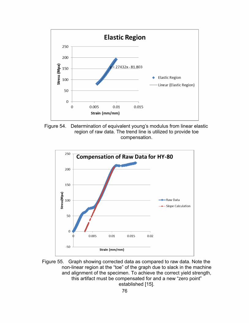
76

Figure 54. Determination of equivalent young’s modulus from linear elastic region of raw data. The trend line is utilized to provide toe

compensation.

Figure 55. Graph showing corrected data as compared to raw data. Note the non-linear region at the “toe” of the graph due to slack in the machine and alignment of the specimen. To achieve the correct yield strength,

this artifact must be compensated for and a new “zero point” established [15].

77

From the equivalent modulus calculated from Figure 28, the machine

compliance was determined:

(1.9) 1 1 1

11 1

27.432 213.831.427


machine

machine

C C C

C

GPa GPaC GPa

Figure 56. Graph illustrated Raw Data (blue dashed line), corrected elastic region (red dot-dashed line) and final, shifted data (black dotted line)

for a carbon fiber composite sample.

78


79

APPENDIX B. ADDITIONAL EXPERIMENTAL RESULTS

A. LLNL CASE 2 “SCRAP” SAMPLE RESULTS

Figure 58. Image of LLNL case 2 “Scrap” samples following impact testing. Similar to actual samples, Scrap samples 1 through 4 show similar failure as case 2 samples 1 through 3. Scrap samples 1 through 4

were struck radially and demonstrated significant delamination between carbon fiber winding layers. Samples 5 through 7 closely

resemble actual case 2 samples 4 and 5. These were struck circumferentially and exhibited fiber breakage. Scrap sample 6 was

mechanically separated by hand to better examine fiber.

Figure 59. Image of LLNL case 2 "Scrap" samples following impact testing.

Table 10. Summary of IZOD test resu lts for set of LLNL case 2 "scrap" samples. Even though geometry does not match lzod ASTM

standards, the standard deviation among

(l)

a. E ro V')

(l) \/)

ro u (l) +-' \/)

0 a.. E 0 u a.. ro ~ u ~

Sample

Number

1

2

3

4

5

6

7

Avg Radia l

STD Dev (Radia l)

Avg Hoop

STD Dev (Hoop)

fracture energy resu lts is small.

Orientation of Strike

Radiai iD

Radiai iD

Radiai iD

Radiai iD

Hoop

Hoop

Hoop

Dimensions (W X D)

(mm)

7.71 X 7.71

7.66x 7.69

7.69 X 7.69

7.7 X 7.69

7.62 X 7.68

7.69 X 7.73

7.71 X 7.72

80

Energy (J)

9.5990

11.8550

11.1660

11.0950

7.9930

7.5724

7.4110

10.9288

0.9505

7.6588

0.3005

J/m

161.4800 1245.0100

201.256 1547.660

188.819 1452.020

187.390 1441.030

136.583 1048.950

127.388 984.710

124.511 961.229

184.7363 1421.4300

16.7079 126.9881

129.4940 998.2963

6.3055 45.4113

81

APPENDIX C. ADDITIONAL ALE3D CODE

A. CFC CODE AND NOTES

Figure 60. Internal (C4) pressure distribution for the thin steel case with no failure model at a time of approximately 5 microseconds.

82

Figure 61. Internal (C4) pressure distribution for the thin steel case with failure model at a time of approximately 5 microseconds.

83

Figure 62. Internal (C4) pressure distribution for the thick steel case with failure model at a time of approximately 5 microseconds.

84

Figure 63. Internal (C4) pressure distribution for the thick steel case with no failure model at a time of approximately 5 microseconds.

85

B. CFC ALE3D INPUT CODE

######################### ######################### # Multi-layer Composite cylinder mesh With C-4 center # Initiation point occurs at TDC of C-4 # # Notes: Reference page numbers are found in ALE3D manual volume 1 or 2 # ALE3D class notes, or ALE3d class examples (as specified) # # Geometry: 4 layers, with fiber orientations of 10, 45, 10, 80 degrees # Composite properties per Kwon’s email (16Jan15) as follows: # model vf Efl vf12 Em vm afl afm # 2 0.50 2.2 0.11 0.035 0.36 5.0 54.0 # shear mod 0.04 # density of LLNL case 2 measured to be (AVG) 1.517 gm/cm^3 # # units: cm, gm, us, Mbar, EU # ######################### ######################### ######################### ######################### # Defined parameter block ######################### ######################### def mres 30 # mesh resolution def dim 3 # dimensionality def boxsize 25. ######################### ######################### # CONTROL parameter block ######################### ######################### CONTROL # Stop time/ stop cycle stoptime 40 #log message every 10 cycles notify 10 # initial time step (V1 pg 157)

86

dtinit 0.01 e_cut 1e-15 # energy cutoff p_cut 1e-15 # pressure cutoff q_cut 1e-15 # artificial viscosity cutoff u_cut 1e-15 # velocity cutoff END ######################### ######################### # HYDRO parameter block ######################### ######################### HYDRO # quadratic q for mixed zones czerox 2.0 # linear q for mixed zones qfbx 0.0 # use sound speed for q calculation for mixed zones linqflag 1 # Set Courant prefactor to just below 2/3 courant .6 # presseq = 0 => do not equilibrate pressure # = 1 => shockImpedance (ss) = 0.0 # = 2 => bulkImpedance (ss**2) = 0.0 # = 3 => everything presseq 3 voidseedopt 1 voidseedcrit damage voidseeddam 0.99 voidseedrelv 1.03 END ######################### ######################### # OUTPUT parameter block ######################### ######################### OUTPUT # plot every until plottime 1 100

87

# plot at cycles 0 and 1 plotac 0 1 # restarts every until dumpcycle 100 100000 # plot tracer locations atcycle 1 plot_tracers 1 atcycle 2 plot_tracers 0 # plot all nodesets until t=1 nodesetplot * 1.0 timehist_fileext .ult timehist_group_begin dataset # tracer particle located at ignition point tracer_fixed tr1 0 0 17.7 timehist p tracer tr1 # Calculating hoop stress derivedvar sxx diff sx p # total x-stress derivedvar syy diff sy p # total y-stress derivedvar sz0 constantzonal 0.0 # Dummy zone variable derivedvar hoop magnitude sxx syy sz0 # Hoop stress assembled from total x & y stresses for theta = 0 45 90 for th = 0 5 10 15 17.7 20 tracer ss<<theta_count>>_<<th_count>> {3.6*cosd(<<theta>>)} {3.6*sind(<<theta>>)} <<th>> timehist fun2j tracer ss<<theta_count>>_<<th_count>> # Time history plot of von mises stress at 0, 45 and 90 deg timehist x tracer ss<<theta_count>>_<<th_count>> # Time history plot of x coordinate at 0, 45, 90 degrees timehist y tracer ss<<theta_count>>_<<th_count>> # Time history plot of y coordinate at 0, 45, 90 degrees timehist p tracer ss<<theta_count>>_<<th_count>> # Time history plot of p at 0, 45, 90 degrees timehist hoop tracer ss<<theta_count>>_<<th_count>> # Time history plot of Hoop Stress (I hope!) 0, 45, 90 degrees endfor endfor timehist_group_end END #########################

88

######################### # ADVECTION parameter block ######################### ######################### ADVECTION # Use “modequipotential” method by B.I. Jun (used in blast3D and vent) rlxmethod 5 # Least restrictive node motion constraint rlxdxopt 3 # Allow relaxation to take place immediately (before node even has velocity) rlxumin 0 # starting position for relaxation calculation is pre-lagrange rlxginit 1 # advection time step control advdtcon 0.5 # advection starts on cycle 1 advcycle 1. # relaxation distance constraint - start small rlxdxmnf 0.05 atcycle 100 rlxdxmnf 0.3 # weight equipotential relaxation based on q (follow shocks) # variable floor min-wgt max-wgt rlxweightvar q 0 1 5 # at 1000 rlxweightvar q 0 1 1 # Convert “lost” Kinetic Energy to internal energy fracke 1 END ######################### ######################### # BURN parameter block ######################### ######################### BURN 2 #burning c4 region #burn velocity (From class example “vent.ain”) for a C4 burn bvel 0.819 # Defining the detonation point detx 0 detz 17.7 dety 0 delay 0 END #########################

89

######################### # MESH ######################## MESH # refining the mesh def res 1 #Notes: Remember that fracture model is mesh-size dependent! # defining variable parameters def steel_rad {3.81} def rad4 {3.7306} def rad3 {3.652} def rad2 {3.5719} def tnt_rad {3.4925} def air_rad 12 def det_rad 0.4 def pipe_length 17.8 def height {boxsize} def frust_length 2 def det_length 1 # multi-shell/layer cylindrical mesh full depicting 3 different regions mcylinder name body type quarter region_rad 2 7 8 9 10 3 region_rad 3 3 3 3 3 3 translate 0 0 0 elems_core {4*res} # blocks in core elems_rad {12*res} {res} {res} {res} {res} {16*res} # blocks in each radius elems_axi {16*res} {(height-pipe_length)*res} # blocks in length radius {tnt_rad} {rad2} {rad3} {rad4} {steel_rad} {air_rad} # assigning parameters to each actual radius length {pipe_length} {height} # actual length ## Change the following boundary condition as you add/subtract layers. The #number is associated with the outermost radius as the outflow surface. “outcyl” #is the outflow nodeset surface r 6 ns outcyl spacetable sp 1.0 xabs 0 xy 0.0 0.0 expr2d x y y/sqrt(x*x+y*y) spacetable cp 1.0 xabs 0 xy 0.0 0.0 expr2d x y x/sqrt(x*x+y*y) END ###########################

90

########################### # BOUNDARY parameter block ########################### ########################### BOUNDARY # Symmetry plane through x=0 (symx) symmetry x 0.0 # Symmetry plane through y=0 symmetry y 0.0 # Symmetry plane through z = 0 (symz) symmetry z 0.0 # Constrain “walls” of box for OUTFLOW nodeset zmax zplane {height} outflow zmax 0.0 0.0 1 1 0 1 #Notes for prevline (inflow energy density) (Relax in x,y,z) (Flag-> no inflow) outflow outcyl 0.0 0.0 0 0 1 1 #Notes for prevline (inflow energy density) (Relax in z only) (Flag-> no inflow) pres_continuous zmax non_reflecting zmax END ######################### ######################### # REGION ######################### ######################### REGION 3 # void/air matname air advinput advmat 1 rlxwmat 1.0 rlxumat 0.0 END #REGION 2 # alum # matname Alum6061 # advinput advmat 1 rlxwmat 4.0 rlxumat 1.0e-3 #END # Kwon’s Composite model: adjusting geometry for cylinder (as opposed to flat # composite plate) with the use # of coordinate transformation and space table.

91

REGION 6 matname umat530 advinput advmat 1 rlxwmat 4.0 rlxumat 1.0 rlxtmat .7 END if gen begin for theta = 10 45 10 80 REGION {6+<<theta_count>>} # Composite matname umat530 advinput advmat 1 rlxwmat 4.0 rlxumat 1.0 rlxtmat .7 reginit f_11 spacetable sp const {-cosd(<<theta>>)} reginit f_12 spacetable cp const { cosd(<<theta>>)} reginit f_13 const { sind(<<theta>>)} reginit f_21 spacetable sp const { sind(<<theta>>)} reginit f_22 spacetable cp const {-sind(<<theta>>)} reginit f_23 const { cosd(<<theta>>)} reginit f_31 spacetable cp const 1. reginit f_32 spacetable sp const 1. reginit f_33 const 0. END endfor endif if { maincode and init } begin for theta = 10 45 10 80 REGION {6+<<theta_count>>} # Composite matname umat530 mergeinput mergeto 6 END endfor endif REGION 2 # C4 matname C4 advinput advmat 1 rlxwmat 2.0 rlxumat 2.000E-05 rlxtmat .7 END REGION 1 matname ms_steel advinput advmat 1 advtmat 0 rlxtmat .5 rlxwmat 10 rlxumat 1 # advinput advmat 1 rlxwmat 0 rlxumat 2.000E-05 # from fragcy.ain file - JC failure model #Johnson-Cook Damage model with statistical distribution for D1 reginit jc_fail_0 gaussian 0.7 0.15 # reginit jc_fail_0 const 0.7 reginit jc_fail_d const 0.0

92

timehist failure vsum timehist damage vsum timehist failure msum timehist damage msum timehist failure mmean timehist damage mmean timehist failure vmean timehist damage vmean END REGION 5 matname void advinput advmat 1 rlxumat 0. rlxwmat 3 END ######################### # MATERIAL ######################### # air MATERIAL Air matinput rho 1.3e-3 e0 2.5e-6 v0 1.0 pmin 0.0 eosvmin 1.e-5 eosvmax 1.e+2 koinput iform 5 isol 0 coef .4 end # Steel MATERIAL Steel matinput rho 7.9 czero 2.0 qfb .15 crq .1 pmin -0.027 epsfail 0.5 v0 1.0 eosvmin 0.5 eosvmax 1.5 use ko 28 end # C-4 (91% RDX) MATERIAL C4 matinput rho 1.650E+00 e0 9.000E-02 v0 1.000E+00 pmin -1.000E+00 czero 2.000E+00 qfb 1.000E-01 crq 1.000E-01 koinput iform 1 coef 6.054E+00 1.112E-01 4.500E+00 1.500E+00 3.700E-01 bhe 3.000E+00 burndl -1. isol 0 END

93

# defining the material of steel MATERIAL ms_steel matinput rho 7.81 e0 0. v0 1. t0 300. cvav 3.559924133e-5 vhlimit 100 linq 1 czero 2. qfb .15 msinput ysmodel 100 elasmodel 1 e_mod 0. poisson 0.3 shr_mod 0.801 lin_press 2.06 lin_temp 3.0e-4 ref_temp 298.3825677 nonlinear 1 etalolim 1. etauplim 3.8 eosmodel 304 rhoc2 1.65 s1 1.49 g0 1.93 a 0.5 ec0 -1.06797724e-02 ec1 -2.06872020e-02 ec2 8.24893246e-01 ec3 -2.39505843e-02 ec4 -2.44522017e-02 ec5 5.38030101e-02 em0 7.40464217e-02 em1 2.49802214e-01 em2 1.00445029e+00 em3 -1.36451475e-01 em4 7.72897829e-03 em5 5.06390305e-02 eosvmin 0.7 eosvmax 1.1 hardmodel 201 y0 0.012 ybet 2. n 0.1 eps_0 0. # Additional feature inserted into J-C damage model; this enables stress # triaxiality; nonlinear from compression to tension until jc_fail_min; # linear behavior from jc_fail_min to (histinit_jc_strength,jc_fail_min); # if not constant then place this in the REGION block. failmodel 400 healable 0 jc_fail_a .5 jc_fail_crit -1.5 jc_fail_min 0.35 histinit jc_strength -1. END MATERIAL void matinput vhlimit 1.01 voidinput ss0 0.2 v0 1.0 e0 0.0 END # Kwon’s Composite Material Model if win32 begin MATERIAL umat530 matinput rho 1.517 e0 0.0 v0 1.0 t0 293. cvav 2.e-5 msinput ysmodel 180 num_constants 8 num_depvars 68 umat_number 1 shear_mod 0.04 bulk_mod 0.8 constants # model vf Efl vf12 Em vm afl afm 2 0.50 2.2 0.11 0.035 0.36 5.0 54.0 library ABAQUSUmat.dll

94

umat_function nps_umat2 elasmodel 99 hardmodel 299 eosmodel 399 failmodel 499 END endif else begin MATERIAL umat530 matinput rho 2.7 e0 0.0 v0 1.0 t0 293. cvav 2.e-5 msinput ysmodel 180 num_constants 8 num_depvars 68 umat_number 1 shear_mod 0.25 bulk_mod 0.8 constants # model vf Efl vf12 Em vm afl afm 2 0.5 0.7238 0.2 0.0275 0.35 5.0 54.0 library ./userumat.so umat_function nps_umat2 elasmodel 99 hardmodel 299 eosmodel 399 failmodel 499 END endif

95

LIST OF REFERENCES

[1] About DTRA/SCC-WMD. (n.d.). Defense Threat Reduction Agency & USSTRATCOM Center for Combating WMD & Standing Joint Force Headquarters-Elimination. [Online]. Available: http://www.dtra.mil/About.aspx. [Accessed 6 Jan 2015].

[2] Agent defeat weapon- NAVY/DTRA. (2013, May 09). Global Security. [Online]. Available: http://www.globalsecurity.org/military/systems/munitions/adw.htm. [Accessed 12 2015 Jan].

[3] National Research Council and the Committee on the Effects of Nuclear Earth-Penetrator and Other Weapons, Effects of Nuclear Earth-Penetrator and Other Weapons, Washington, DC: The National Academies Press, 2005.

[4] J. Molitoris, Image Courtesy of LLNL EMC via private communication, Livermore, CA: Lawrence Livermore National Laboratory, Jan. 2015.

[5] A. T. Nettles, “Instrumented impact and residual tensile strength testing of eight-ply carbon/epoxy specimens,” NASA., Huntsville, Al, Rep. #2981, Jan. 1990.

[6] P. Ma, G. Jiang, Q. Chen, X. Maio and S. Zhao, “Compression behaviors of carbon woven composites with carbon nanotube-filled epoxy resin under high strain rates,” Textile Research Journal, vol. 85, no. 1, pp. 36–50, Jan. 2015.

[7] S. Thiruppukuzhi and C. Sun, “Testing and modeling high strain rate behavior of polymeric composites,” Composites, vol. 29, no. 5, pp. 519-672, Sept. 1998.

[8] D. Siromani, J. Awerbuch, and T.-M. Tan, “Finite element modeling of the crushing behavior of thin-walled CFRP tubes under axial compression,” Composites, vol. 64, pp. 50-58, Apr. 2014.

[9] N. Saad, M. Hamzah, and A. Hamzah, (2014). “Experimental and numerical simulation of impact fracture toughness of polyphenylene sulfide basis composite material. [Online]. Available: https://www.uobabylon.edu.iq/uobcoleges/fileshare/articles/... repository1_publication2491_29_5234.pdf

[10] M. Kumar, M. R. Devaraj, and H. LakshmiNarayana, “Finite element modelling for numerical simulation of charpy impact test on materials,” in International Conference on Challenges and Opportunities in Mechanical Engineering, Industrial Engineering and Management Studies, UNK, 2012.

96

[11] R. Anbazhagan and G. Ragamani, “Modelling and analysis of impact properties on polyurethane composites using FEA,” International Journal of ChemTech Research, vol. 6, no. 1, pp. 114–123, 2014.

[12] C. Alexander, C. Key, and S. Schumacher, “Dynamic response and modeling of a carbon fiber-epoxy composite subject to shock loading,” Journal of Applied Physics, vol. 114, pp. 1–10, 2013.

[13] B. Baker, “Processing, microstructure and material property relationships following friction stir welding of oxide dispersion strengthened steels. (Doctoral disseration),” Calhoun Institutional Archive of the Naval Postgraduate School., Monterey, CA, 2013.

[14] P. Han, Tensile Testing, Materials Park, Ohio: ASM International, 1992, pp 1-12.

[15] Standard Test Method for Compressive Properties of Rigid Plastics, ASTM Standard D695, 2010.

[16] W. D. Callister, Materials Science and Engineering an Introduction, New York, NY: John Wiley & Sons, 2003.

[17] Jordan, Foley and Siviour, “Mehcanical properties of EPON 826/DEA epoxy,” Air Force Research Lab., Eglin AFB, FL, Rep. AFRL-RW-EG-TP-2008-7418, Aug. 2008.

[18] J. Courm, R. Battiste, K. Lui, and M. Ruggles, “Basic properties of reference crossply carbon-fiber composite,” Oak Ridge Nataional Lab., Oak Ridge, TN, Rep. ORNL/TM-2000/29. Feb. 2000.

[19] American Society of Mechanical Engineers, “Split-Hopkinson Pressure Bar Apparatus: An Historic Mechanical Engineering Landmark,” Southwest Research Institute, San Antonio, TX, 2006.

[20] Split-Hopkinson pressure bar testing. (n.d.). Department of Materials Science and Engineering, University of Illinois and Urbana-Champaign. [Online]. Available: http://hrdg.matse.illinois.edu/hopbar.html. [Accessed 16 Jan 2015].

[21] Standard Test Methods for Determining the Izod Pendulum Impact Resistance of Plastics. ASTM Standard D256, 2002.

[22] M. Manahan and R. Stonesifer, “The difference between total absorbed energy measured using an instrumented striker and that obtained using an optical encoder,” in Pendulum Impact Testing; A Century of Progress, ASTM STP 1380, West Conshohocken, PA, American Society for Testing and Materials, 1999.

97

[23] Model IT 504 Pendulum Impact System Instruction Book, #04-03, Tinius Olson, Horsham, PA, 2012.

[24] H.H. Lee, Finite Element Simulations with ANSYS Workbench 14; Theory, Applications, Case Studies, Mission, KS: SDC Publications, 2011.

[25] Lawrence Livermore National Laboratory ALE3D Team, ALE3D User’s Manual, 4.22.x ed., Livermore, Ca: LLNL, 2014.

[26] M. S. Park and Y. W. Kwon, “Elastoplastic micromechanics model for multiscale analysis of MMC structures,” Computers and Structures, vol. 123, pp. 28–38, 2013.

[27] Y. Kwon and M. Park, “Versatile micromechanics model for multiscale analysis of composite structures,” Applied Composite Materials, vol. 20, no. 4, pp. 673–692, 2013.

[28] J. Molitoris, H. Andreski, W. Howard, M. DeHaven, R. Simpson, and R. Doherty, “Combustion evaluation of PBXIH-135, Tritonal and TNT for thermobarics and Enhanced Blast,” Lawrence Livermore National Laboratory Energetic Materials Center, Livermore, CA, Rep. UCRL-TR-202329, 2004.

[29] J. Molitoris, J. Batteux, R. Garza, J. Tringe, and P. Souers, “Mix and Instability Growth from Oblique Shock,” Lawrence Livermore National Laboratory, Energetic Materials Center, Livermore, CA, Rep. LLNL-PROC-491379, Jun. 2011.

98


99

INITIAL DISTRIBUTION LIST

1. Defense Technical Information Center Ft. Belvoir, Virginia 2. Dudley Knox Library Naval Postgraduate School Monterey, California

NAVAL POSTGRADUATE SCHOOLFigure 24. ANSYS Explicit Dynamic refined mesh and support constraints for...

Documents

Transcript of NAVAL POSTGRADUATE SCHOOLFigure 24. ANSYS Explicit Dynamic refined mesh and support constraints for...