NAVAL POSTGRADUATE SCHOOL - Defense … traditional method designed 9-ball, 12-ball, 18-ball, and...

NAVAL

POSTGRADUATE SCHOOL

MONTEREY, CALIFORNIA

THESIS

Approved for public release; distribution is unlimited

OPTIMIZING COVERAGE AND REVISIT TIME IN SPARSE MILITARY SATELLITE CONSTELLATIONS: A

COMPARISON OF TRADITIONAL APPROACHES AND GENETIC ALGORITHMS

by

Douglas J. Pegher and

Jason A. Parish

September 2004

Thesis Advisor: Charles Racoosin Second Reader: Donald Danielson

THIS PAGE INTENTIONALLY LEFT BLANK

i

REPORT DOCUMENTATION PAGE Form Approved OMB No. 0704-0188 Public reporting burden for this collection of information is estimated to average 1 hour per response, including

the time for reviewing instruction, searching existing data sources, gathering and maintaining the data needed, and completing and reviewing the collection of information. Send comments regarding this burden estimate or any other aspect of this collection of information, including suggestions for reducing this burden, to Washington headquarters Services, Directorate for Information Operations and Reports, 1215 Jefferson Davis Highway, Suite 1204, Arlington, VA 22202-4302, and to the Office of Management and Budget, Paperwork Reduction Project (0704-0188) Washington DC 20503. 1. AGENCY USE ONLY (Leave blank)

2. REPORT DATE September 2004

3. REPORT TYPE AND DATES COVERED Master’s Thesis

4. TITLE AND SUBTITLE: Optimizing Coverage and Revisit Time in Sparse Military Satellite Constellations: A Comparison of Traditional Approaches and Genetic Algorithms 6. AUTHOR(S) Douglas J. Pegher and Jason A. Parish

5. FUNDING NUMBERS

7. PERFORMING ORGANIZATION NAME(S) AND ADDRESS(ES) Naval Postgraduate School Monterey, CA 93943-5000

8. PERFORMING ORGANIZATION REPORT NUMBER

9. SPONSORING /MONITORING AGENCY NAME(S) AND ADDRESS(ES)

N/A

10. SPONSORING/MONITORING AGENCY REPORT NUMBER

11. SUPPLEMENTARY NOTES The views expressed in this thesis are those of the author and do not reflect the official policy or position of the Department of Defense or the U.S. Government. 12a. DISTRIBUTION / AVAILABILITY STATEMENT

Approved for public release; distribution is unlimited 12b. DISTRIBUTION CODE A

13. ABSTRACT (maximum 200 words) Sparse military satellite constellations were designed using two methods: a traditional approach and

a genetic algorithm. One of the traditional constellation designs was the Discoverer II space based radar. Discoverer II was an 8 plane, 24 satellite, Low Earth Orbit (LEO), Walker constellation designed to provide high-range resolution ground moving target indication (HRR-GMTI), synthetic aperture radar (SAR) imaging and high resolution digital terrain mapping. The traditional method designed 9-ball, 12-ball, 18-ball, and 24-ball Walker constellations. The genetic algorithm created constellations by deriving a phenotype from a triploid genotype encoding of orbital elements. The performance of both design methods were compared using a computer simulation. The fitness of each constellation was calculated using maximum gap time, maximum revisit time, and percent coverage. The goal was to determine if one design method would consistently outperform the other. The genetic algorithm offered a fitness improvement over traditional constellation design methods in all cases except the 24-ball constellation where it demonstrated comparable results. The genetic algorithm improvement over the traditional constellations increased as the number of satellites per constellation decreased. A derived equation related revisit time to the number of ship tracks maintained.

15. NUMBER OF PAGES

145

14. SUBJECT TERMS Constellation design, space based radar, synthetic aperture radar, ground moving target indicator, surface moving target indicator, genetic algorithms 16. PRICE CODE 17. SECURITY CLASSIFICATION OF REPORT

Unclassified

18. SECURITY CLASSIFICATION OF THIS PAGE

Unclassified

19. SECURITY CLASSIFICATION OF ABSTRACT

Unclassified

20. LIMITATION OF ABSTRACT

UL

NSN 7540-01-280-5500 Standard Form 298 (Rev. 2-89) Prescribed by ANSI Std. 239-18

ii


iii

Approved for public release; distribution is unlimited

OPTIMIZING COVERAGE AND REVISIT TIME IN SPARSE MILITARY SATELLITE CONSTELLATIONS: A COMPARISON OF TRADITIONAL

APPROACHES AND GENETIC ALGORITHMS

Douglas J. Pegher Lieutenant, United States Navy

B.A., Edinboro University of Pennsylvania, 1993

Jason A. Parish Lieutenant, United States Navy

B.S., Rensselaer Polytechnic Institute, 1997

Submitted in partial fulfillment of the requirements for the degree of

MASTER OF SCIENCE IN SPACE SYSTEMS OPERATIONS

from the

NAVAL POSTGRADUATE SCHOOL

September 2004

Authors: Douglas J. Pegher Jason A. Parish Approved by: Charles Racoosin

Thesis Advisor

Donald Danielson Second Reader Rudy Panholzer Chairman, Space Systems Academic Group

iv


v

ABSTRACT

Sparse military satellite constellations were designed using two methods:

a traditional approach and a genetic algorithm. One of the traditional

constellation designs was the Discoverer II space based radar. Discoverer II was

an 8 plane, 24 satellite, Low Earth Orbit (LEO), Walker constellation designed to

provide high-range resolution ground moving target indication (HRR-GMTI),

synthetic aperture radar (SAR) imaging and high resolution digital terrain

mapping. The traditional method designed 9-ball, 12-ball, 18-ball, and 24-ball

Walker constellations. The genetic algorithm created constellations by deriving a

phenotype from a triploid genotype encoding of orbital elements. The

performance of both design methods were compared using a computer

simulation. The fitness of each constellation was calculated using maximum gap

time, maximum revisit time, and percent coverage. The goal was to determine if

one design method would consistently outperform the other. The genetic

algorithm offered a fitness improvement over traditional constellation design

methods in all cases except the 24-ball constellation where it demonstrated

comparable results. The genetic algorithm improvement over the traditional

constellations increased as the number of satellites per constellation decreased.

A derived equation related revisit time to the number of ship tracks maintained.

vi


vii

TABLE OF CONTENTS I. TRADITIONAL CONSTELLATION DESIGN.................................................. 1

A. HISTORY ............................................................................................. 1 1. Origin ........................................................................................ 1 2. Copernicus............................................................................... 2 3. Kepler ....................................................................................... 2 4. Newton...................................................................................... 2

B. ORBIT DETERMINATION ................................................................... 3 1. Classic Orbital Elements (COE).............................................. 3

a. Semimajor Axis (a)........................................................ 3 b. Eccentricity (e) .............................................................. 4 c. Inclination (i).................................................................. 4 d. Right Ascension of the Ascending Node (Ω )............. 4 e. Argument of Perigee (ω ) ............................................. 4 f. True Anomaly ( ν ) ......................................................... 4

2. Orbit Selection ......................................................................... 4 a. Low Earth Orbit (LEO) .................................................. 5 b. Geosynchronous Orbit (GEO)...................................... 5 c. Medium Earth Orbit (MEO) ........................................... 5 d. Highly Elliptical Orbit (HEO)......................................... 6

3. Design Process........................................................................ 6 a. Establish Orbit Types ................................................... 6 b. Determine Orbit-related Mission Requirements......... 6 c. Assess Applicability of Specialized Orbits................. 7 d. Evaluate Whether a Single Satellite or a

Constellation is Needed ............................................... 8 e. Perform Mission Orbit Design Trades......................... 8 f. Evaluate Constellation Growth and

Replenishment or Single-satellite Replacement Strategy.......................................................................... 8

g. Assess Retrieval or Disposal Options ........................ 9 h. Create ∆V Budget.......................................................... 9 i. Determine Launch Options and Cost .......................... 9 j. Document and Iterate ................................................. 10

C. CONSTELLATION DESIGN CONSIDERATIONS............................. 10 1. Parameters ............................................................................. 10

a. Swath Width ................................................................ 10 b. Altitude......................................................................... 10 c. Inclination .................................................................... 10 d. Node Spacing .............................................................. 10

2. Coverage ................................................................................ 10 3. Number of Satellites .............................................................. 11

viii

4. Launch Options ..................................................................... 11 5. Environment........................................................................... 11 6. Stationkeeping ....................................................................... 11 7. Collision Avoidance .............................................................. 12 8. Constellation Build-up, Replenishment, and End-of-Life... 12 9. Number of Orbit Planes......................................................... 12

D. PATTERNS ........................................................................................ 12 1. Geosynchronous Constellations.......................................... 12 2. Streets of Coverage Constellations ..................................... 12 3. Walker Constellations ........................................................... 13 4. Elliptical Orbit Patterns ......................................................... 14 5. Other Constellation Patterns ................................................ 14

E. SUMMARY......................................................................................... 15 1. Process................................................................................... 15

a. Establish Constellation-related mission requirements ............................................................... 15

b. Do All Single Satellite Orbit Trades Except Coverage...................................................................... 15

c. Do Trades Between Swath Width, Coverage, and Number of Satellites ................................................... 15

d. Evaluate Ground Track Plots ..................................... 15 e. Adjust Inclination and In-plane Phasing ................... 15 f. Review the Rules of Constellation Design................ 15 g. Document Reasons for Choices and Iterate............. 15

2. Design Factors....................................................................... 15 a. Principal....................................................................... 15 b. Secondary.................................................................... 15

II. GENETIC ALGORITHMS ............................................................................. 17 A. THEORY ............................................................................................ 17 B. HISTORY ........................................................................................... 17 C. PROCESS.......................................................................................... 19 D. APPLICATIONS................................................................................. 20 E. VOCABULARY .................................................................................. 21

III. THE TRADITIONAL MODEL........................................................................ 23 A. BACKGROUND ................................................................................. 23 B. SPACE BASED RADAR (SBR)......................................................... 23

1. Imaging radar ......................................................................... 23 a. Basics .......................................................................... 23 b. Detection...................................................................... 25 c. Range Resolution........................................................ 26 d. Signal Shape ............................................................... 26 e. Azimuth Resolution .................................................... 27 f. Resolution ................................................................... 27

2. Synthetic Aperture Radar (SAR)........................................... 27 3. Ground Moving Target Indicator (GMTI) .............................. 29

ix

4. Future ..................................................................................... 32 a. The Requirements Dilemma....................................... 32 b. From Scratch............................................................... 33 b. Reality .......................................................................... 33

C. DISCOVERER II................................................................................. 34 1. Background............................................................................ 35 2. Capabilities............................................................................. 35 3. General Characteristics ........................................................ 36 4. Reality..................................................................................... 37

D. THE MODEL ...................................................................................... 38

IV. THE GENETIC ALGORITHM ....................................................................... 39 A. BACKGROUND ................................................................................. 39 B. THE GENETIC ALGORITHM............................................................. 41

1. Overview................................................................................. 41 2. Create Initial Population........................................................ 42 3. Calculate Phenotype ............................................................. 42 4. Evaluate Fitness .................................................................... 43 5. Scale Fitness.......................................................................... 44 6. Crossover Engine and Crossover ........................................ 45 7. Mating Coupler and Create Offspring .................................. 47 8. Mutation Engine and Mutation.............................................. 48 9. Finishing the Example........................................................... 49

C. PARAMETERS .................................................................................. 50 1. Population Size and Number of Generations ...................... 50 2. Crossover and Mutation Probability .................................... 51

C. STK INTERFACE............................................................................... 52

V. CONSTELLATION COMPARISON .............................................................. 53 A. BACKGROUND ................................................................................. 53 B. THE PROCESS.................................................................................. 53

1. Constraints............................................................................. 53 2. Data Points ............................................................................. 53 3. Measurements of Fitness...................................................... 55

a. Average Gap................................................................ 56 b. Maximum Revisit......................................................... 56 c. Percent Coverage ....................................................... 56 d. Weight .......................................................................... 56 e. Overall Fitness ............................................................ 57

C. RESULTS........................................................................................... 57 1. 9-ball Constellations.............................................................. 58 2. 12-ball Constellations............................................................ 60 3. 18-ball Constellations............................................................ 63 4. 24-ball Constellations............................................................ 66

D. SUMMARY......................................................................................... 69

VI. THE BENEFITS OF SUPERIORITY ............................................................. 73

x

A. THE THREAT..................................................................................... 73 B. A POSSIBLE SOLUTION .................................................................. 74

1. The Theory ............................................................................. 74 2. The Math................................................................................. 77 3. The Solution........................................................................... 80

C. CONCLUSION ................................................................................... 83 D. FURTHER STUDY ............................................................................. 83

1. Caveat..................................................................................... 83 2. Next Steps .............................................................................. 84

LIST OF REFERENCES.......................................................................................... 85

APPENDIX A GENETIC ALGORITHM CODE............................................... 89

APPENDIX B CONSTELLATION ORBITAL ELEMENTS........................... 111 A. 9-BALL CONSTELLATIONS........................................................... 111

1. Genetic Algorithm Design................................................... 111 2. 3-plane Walker ..................................................................... 111

B. 12-BALL CONSTELLATIONS......................................................... 111 1. Genetic Algorithm Design................................................... 111 2. 4-plane Walker ..................................................................... 112

C. 18-BALL CONSTELLATIONS......................................................... 112 1. Genetic Algorithm Design................................................... 112 2. 6-plane Walker ..................................................................... 113

D. 24-BALL CONSTELLATIONS......................................................... 113 1. Genetic Algorithm Design, Independent Case .................. 113 2. Genetic Algorithm Design, Dependent Case..................... 114 3. 4-plane Walker ..................................................................... 115 4. 6-plane Walker ..................................................................... 116 5. 8-plane Walker, Discoverer II .............................................. 117 6. 12-plane Walker ................................................................... 118

APPENDIX C CONSTELLATION FITNESS CALCULATIONS................... 119 A. 9-BALL CONSTELLATIONS........................................................... 119

1. Genetic Algorithm Design................................................... 119 2. 3-plane Walker ..................................................................... 119

B. 12-BALL CONSTELLATIONS......................................................... 120 1. Genetic Algorithm Design................................................... 120 2. 4-plane Walker ..................................................................... 120

C. 18-BALL CONSTELLATIONS......................................................... 121 1. Genetic Algorithm Design................................................... 121 2. 6-plane Walker ..................................................................... 121

D. 24-BALL CONSTELLATIONS......................................................... 122 1. Genetic Algorithm Design, Independent Case .................. 122 2. Genetic Algorithm Design, Dependent Case..................... 122 3. 4-plane Walker ..................................................................... 123 4. 6-plane Walker ..................................................................... 123 5. 8-plane Walker, Discoverer II .............................................. 124

xi

6. 12-plane Walker ................................................................... 124

INITIAL DISTRIBUTION LIST ............................................................................... 125

xii


xiii

LIST OF FIGURES

Figure 1. Streets of Coverage Constellation [From 3]........................................ 13 Figure 2. Walker Constellation [From 4] ............................................................ 14 Figure 3. Definitions of Terms for Imaging Radar [From 12].............................. 25 Figure 4. Radar Pulse [From 13] ....................................................................... 26 Figure 5. SAR Effective Antenna Length [From 12]........................................... 28 Figure 6. SAR/GMTI Composite [From 14]........................................................ 30 Figure 7. Joint STARS Coverage In Operation Desert Storm [From 15] ........... 31 Figure 8. Genetic Algorithm Pseudocode .......................................................... 42 Figure 9. Meta-GA Data .................................................................................... 52 Figure 10. Distribution of Land and Water by Latitude [From 25] ........................ 54 Figure 11. Weight by Latitude.............................................................................. 57 Figure 12. Comparison of 9-ball Constellation Average Revisit Time.................. 58 Figure 13. Comparison of 9-ball Constellation Maximum Gap Time.................... 59 Figure 14. Comparison of 9-ball Constellation Percent Coverage....................... 60 Figure 15. Comparison of 12-ball Constellation Average Revisit Time................ 61 Figure 16. Comparison of 12-ball Constellation Maximum Gap Time.................. 62 Figure 17. Comparison of 12-ball Constellation Percent Coverage..................... 63 Figure 18. Comparison of 18-ball Constellation Average Revisit Time................ 64 Figure 19. Comparison of 18-ball Constellation Maximum Gap Time.................. 65 Figure 20. Comparison of 18-ball Constellation Percent Coverage..................... 66 Figure 21. Comparison of 24-ball Constellation Average Revisit Time................ 67 Figure 22. Comparison of 24-ball Constellation Maximum Gap Time.................. 68 Figure 23. Comparison of 24-ball Constellation Percent Coverage..................... 69 Figure 24. Geometry between the Earth, Satellite, and Target [After 5] .............. 77 Figure 25. 24-ball Walker Performance ............................................................... 81 Figure 26. 18-ball GA Performance ..................................................................... 81 Figure 27. 12-ball GA Performance ..................................................................... 82 Figure 28. 9-ball GA Performance ....................................................................... 82

xiv


xv

LIST OF TABLES

Table 1. Bitwise Comparison............................................................................ 43 Table 2. Fitness Weighting by Latitude Land Area ........................................... 55 Table 3. GMTI Sensor Data.............................................................................. 56 Table 4. Summary of Fitness Scores for Designed Constellations................... 70 Table 5. Search Rate Data and Equations ....................................................... 79

xvi


xvii

ACKNOWLEDGMENTS Jason and Doug would like to extend our thanks to Prof. Charlie Racoosin

for his guidance, from finding a suitable satellite system to his insightful

comments, all of which pushed, pulled, and prodded both of us through the

discovery and learning process which is this thesis. We would like to thank Prof.

David Trask for his knowledge and expertise in translating what a sky full of SBR

satellites provides the war fighter. We would like to thank Prof. Don Danielson

for his insight and advice in completing this thesis. Doug extends his thanks to

Dan Sakoda and George Zolla at NPS for their advice and assistance with STK

and Visual Basic. Doug would also like to acknowledge the contributions of Paul

Castleburg and John McCarthy of Toyon Research who provided information on

modeling and simulation of SBR.

Finally, we would be remiss if we did not acknowledge the loving support

of our families.

xviii


1

I. TRADITIONAL CONSTELLATION DESIGN

A. HISTORY 1. Origin Scientists have been studying astrodynamics (the motion of natural and

human-made bodies in outer space) since the ancient era. Some definitions of

astrodynamics leave out the "natural" portion, establishing the origin of

astrodynamics on 10 October 1946 with the launch of the V2 rocket into space or

04 October 1957 with the launch and subsequent orbit of Sputnik 1. However,

regardless of the definition, astronomers contributed to the study of

astrodynamics beginning about 200 A.D.

The Chaldeans were probably the first to develop astrology. They

developed the Saros cycle by measuring the time between eclipses. Focusing

on the moon rather than the sun, the Babylonians developed the lunar month by

observing the phases of the moon.

The first recognized astrologer was probably Thales of Miletus (c. 640-546

B.C.). Thales determined the length of the year, predicted eclipses, founded the

Ionian school of astronomy and philosophy and taught that the world was

spherical. Pythagorous (569-470 B.C.) taught astronomy and philosophy. He

believed that comets revolved around the sun and the earth rotated about its own

axis. Aristarchus (310-250 B.C.) was possibly the first person to suggest the

earth rotated around the sun. Eratosthenes (275-194 B.C.) was the first to

calculate the radius of the earth accurately.

Hipparchus (c. 161-126 B.C.) developed spherical geometry and also

declared the sun to be the center of the universe. In addition, he began

cataloging stars based on brightness. Without the aid of instruments, Hipparchus

categorized over 1000 stars based on magnitude, separating each star into one

of six categories of brightness separated by about 2.5 times the brightness of the

previous star. Hipparchus also developed theories of orbital motion.

2

Claudius Ptolemaceus (100-170 A.D.) continued Hipparchus' work.

Unfortunately he was not exposed to earlier work declaring the sun as the center

of the universe. Instead, he published a 13-volume work explaining the motion of

celestial bodies around the earth.

There was a large gap of time between Ptolemaceus' work and the next

significant scientific contribution to astrodynamics provided by Nicholas

Copernicus (1473-1543).

2. Copernicus Copernicus proposed a Sun-centered solar system. He also disagreed

with Ptolemaceus in some numbers and data and the motion of the planets.

Unfortunately, Copernicus' theories were controversial at the time and,

consequently, his work was not published until he was near death. It is thought

that Copernicus theorized elliptical motion but the sections were not included in

his work.

3. Kepler Johann Kepler (1571-1630) determined how to relate mean and true

anomalies in the orbit to time in order to predict future occurrences for planets.

Using Copernicus' Sun-centered solar system as a starting point, Kepler

developed three laws to describe the kinematics of motion of celestial bodies:

1. The orbit of each planet is an ellipse with the Sun at one focus.

2. The line joining the planet to the Sun sweeps out equal areas in

equal times.

3. The square of the period of a planet is proportional to the cube of

its mean distance to the Sun.

Kepler printed three books; Astronomia Nova (1609) containing his first

two laws, De Cometis (1618) about comets, and Harmonices Mundi Libri V

(1619) describing physical motion.

4. Newton Isaac Newton (1642-1727) discovered the mathematical solution to the

dynamics of motion. Newton explained the law of gravitational attraction that

3

accounts for the elliptical motion of planets using an inverse square law. At

Edmond Halley's urging (and funding), Newton published Philosophiate Naturalis

Principia Mathematica in 1687. In his book, referred to as the Principia, Newton

introduced his three laws of motion:

1. Every body continues in its state of rest, or of uniform motion in a

right [straight] line, unless it is compelled to change that state by

forces impressed upon it.

2. The change of motion is proportional to the motive force impressed

and is made in the direction of the right line in which that force is

impressed.

3. To every action there is always opposed an equal reaction: or, the

mutual actions of two bodies upon each other are always equal and

directed to contrary parts.

Newton's Universal Law of Gravitation - in combination with his three laws

of motion - allowed scientists to model planetary and satellite motion.

Joseph Louis Lagrange (1736-1813), Leonhard Euler (1707-1783), Carl

Gustav Jacob Jacobi (1804-1851) and Henri Poincaré (1854-1912) also made

significant contributions to the study of astrodynamics, particularly in modeling

three body object interaction. [1]

B. ORBIT DETERMINATION 1. Classic Orbital Elements (COE) Six orbital elements are used to define a satellite's orbit for positioning and

tracking. Once all of the COE are known, the orbit size, shape, orientation and

location of the spacecraft in that orbit can be determined.

a. Semimajor Axis (a) The semimajor axis is used to determine the size of the orbit. The

semimajor axis is half the distance along the long axis of the ellipse around which

the spacecraft travels. For circular orbits, the semimajor axis is simply the radius

of the circle made by the orbiting satellite.

4

b. Eccentricity (e) The eccentricity is used to determine the shape of the orbit. The

eccentricity is the ratio of the distance between the two foci and the semimajor

axis. The eccentricity is 0 for a circle and 0 < e < 1 for an ellipse.

c. Inclination (i) The inclination is used to determine the tilt of the orbit. The

inclination is the angle between the fundamental plane of the coordinate system

(the equatorial plane in an earth centered system) and the orbital plane. An

equatorial orbit has an inclination of 0° or 180°, a polar orbit has an inclination of

90°, a direct or prograde orbit has an inclination of 0° ≤ i < 90°, and an indirect or

retrograde orbit has an inclination of 90° < i ≤ 180°.

d. Right Ascension of the Ascending Node (Ω ) The right ascension of the ascending node is used to determine the

angular orientation of the orbit relative to some principal direction. The right

ascension of the ascending node is the angle from the vernal equinox (a line

drawn from earth through the sun on the first day of Spring) to the ascending

node (the intersection of the orbital plane and the fundamental plane as the

spacecraft travels from the Southern Hemisphere to the Northern Hemisphere).

e. Argument of Perigee (ω ) The argument of perigee is used to determine the orbital ellipse’s

orientation within the orbital plane. The argument of perigee is the angle, along

the orbital path, between the ascending node and perigee (the point of the orbit

closest to earth).

f. True Anomaly ( ν ) The true anomaly is used to determine the spacecraft's location

within the orbit. The true anomaly is the angle, along the orbital path, between

perigee and the spacecraft's position vector (from earth's center to the satellite)

measured in the direction of the spacecraft's motion. [2]

2. Orbit Selection Engineers spend many hours in the design process determining

spacecraft orbital parameters. Orbit altitudes are often of primary interest –

5

based on mission requirements – and are generally grouped into one of four

categories based on the distance from earth the spacecraft will travel while on

orbit.

a. Low Earth Orbit (LEO) The Low Earth Orbit includes all orbits from an altitude of a few

hundred kilometers to the Van Allen Radiation Belts ( 1500 km). They generally

have a period of approximately 90 minutes and have more than ten revolutions

per day. Some advantages of LEO orbits are: better resolution for remote

sensing, less expensive launch costs, and less power needed to transmit signals.

Some disadvantages are: limited viewing area, many satellites needed to

achieve continuous global coverage, and shorter spacecraft lifetimes due to drag

and orbit decay.

b. Geosynchronous Orbit (GEO) The Geosynchronous Orbit is at an altitude of nearly 36,000 km.

GEO orbits have a 24 hour period and revolve with the earth. Some advantages

of GEO are: the ability to "stare" at one area of the earth, approximately 1/3 earth

coverage with one satellite and global coverage with as few as five satellites

(lower satellite construction cost than LEO to achieve the same coverage).

Some disadvantages of GEO are: very poor remote sensing resolution, high

power needed to transmit to earth, large antennas needed for sensing, and

expensive to get to orbit.

c. Medium Earth Orbit (MEO) The Medium Earth Orbit includes all orbits from the Van Allen Belts

to an altitude around 30,000 km. However, typically, MEO satellites are at an

altitude of just over 20,000 km. They have a 12 hour period with two revolutions

per day. MEO orbits have all of the advantages and disadvantages of both LEO

and GEO. As compared to LEO, MEO satellites are able to see a greater

percentage of the earth at a time and therefore require fewer satellites to cover

the globe (The Global Positioning System uses 24 satellites for four-fold global

coverage). However, MEO satellites require more power to transmit signals to

earth and cannot achieve the same remote sensing resolution as LEO sensors.

6

d. Highly Elliptical Orbit (HEO) A Highly Elliptical Orbit is one that does not fit well into one of the

previous classifications. They are characterized by large values for eccentricity

or large differences between the perigee and apogee altitudes. Typically HEO

pass through all of the other orbital regimes, for example the Molniya orbit has a

perigee of 500 km and an apogee of 39,850 km. Molniya orbits have a 12 hour

period with two revolutions per day and an inclination of 63.4°. Satellites in HEO

orbits are typically at an inclination of 63.4°; at this inclination the perigee

remains fixed, at other inclinations the perigee rotates. The advantage of HEO is

a long dwell time at apogee. The disadvantage of HEO is very limited coverage

near perigee.

3. Design Process a. Establish Orbit Types Step 1 involves examining the four types of orbits. The Earth-

referenced and space-referenced orbits are operational orbits (the satellite/s will

remain in the orbit for the majority of their lifetime). The transfer and parking

orbits are used to get the satellites to their operational orbits

(1) Earth-referenced orbits are used to cover the earth

(The Global Positioning System).

(2) Space-referenced orbits are used to cover space (the

Hubble Space Telescope).

(3) Transfer orbits are used to transition a satellite from

one orbit to another (Hohmann Transfer).

(4) Parking orbits are used as a transition orbit between

the initial and final orbit.

b. Determine Orbit-related Mission Requirements Step 2 involves examining the mission requirements. Earth-

referenced mission requirements drive the orbit to one of the orbital regimes

described above (LEO, MEO, HEO or GEO). For example, a need for high

resolution pictures would drive the orbit to LEO but a need for long dwell times

would drive the orbit to HEO or GEO.

7

Three other orbits that must be considered are transfer, parking

and reference orbits. Transfer orbits are used to get the spacecraft where it is

needed when it is needed. Design of the transfer orbit is generally

uncomplicated with cost (∆V or propellant) as the driver.

Parking orbits – or storage orbits - are used to provide a spacecraft

a place to linger while waiting for transfer into the ultimate orbit destination.

Often parking orbits are sparsely populated orbits at an altitude high enough to

minimize drag but low enough to retrieve the spacecraft easily. Some typical

spacecraft in parking orbits are on-orbit spares, spacecraft being tested following

launch and spacecraft waiting for the proper conditions to be met before

transferring to the mission orbit.

Mission orbits are either earth referenced of space referenced.

Earth-referenced orbits allow the spacecraft sensors to provide coverage of the

earth or the space near earth. Space-referenced orbits allow the spacecraft

sensors to point toward space. Often, for space-referenced orbits, specific orbit

parameters are not crucial.

c. Assess Applicability of Specialized Orbits Step 3 involves examining whether the unique characteristics of a

specialized orbit offers an advantage over traditional LEO, MEO and GEO.

Usually the advantage must be significant to offset the added cost usually

associated with specialized orbits.

Some specialized orbits include:

• Geostationary. A geosynchronous orbit with inclination and eccentricity approximately zero. Geostationary satellites maintain their relative position fixed over one geographic area.

• Sun-synchronous. The orbit rotates as the earth rotates about the sun. Consequently, the orbit maintains a constant orientation with the sun and allows the satellite to cross the equator at the same local time each pass.

• Polar. A 90° inclination orbit used to provide polar coverage.

• Molniya. A highly elliptical, highly inclined orbit which provides coverage to northern latitudes where geostationary satellites do not.

8

• Repeating ground track. An orbit for which the ground track of the satellite will repeat itself after one or more days.

• Frozen. Stable orbits with low eccentricity and an argument of perigee of 90° or 270°.

• Super Synchronous. An Earth orbit with a semi-major axis greater than a geosynchronous orbit. d. Evaluate Whether a Single Satellite or a Constellation is

Needed Step 4 involves determining whether a single satellite is sufficient or

an entire constellation is required. As a rule, single satellites are less expensive

and therefore desired if they can accomplish the mission. However, single

satellites are often complex and provide no redundancy (if you lose the satellite

you cannot accomplish the mission). A constellation of small inexpensive

satellites may be a better solution.

e. Perform Mission Orbit Design Trades Step 5 involves choosing an orbit based on the mission the satellite

will be asked to perform. Some considerations when selecting orbits are;

coverage, sensitivity or performance, environment and survivability, launch

capability, ground communications, orbit lifetime, and legal or political

constraints.

Some missions can be completed regardless of altitude. In this

case, mission requirements must be weighted based on preference. For

example, communications can be done from all altitudes. An adequately

populated LEO constellation, using several satellites and relay, could enable

communications between two users anywhere on the globe. A GEO satellite

constellation of 5 inclined satellites could do the same. The trade may be the

cost of populating a LEO constellation versus populating a constellation in GEO.

f. Evaluate Constellation Growth and Replenishment or Single-satellite Replacement Strategy

Step 6 involves determining how to keep the constellation useful.

Satellite constellations are generally populated a few satellites at a time. Ideally,

the constellation will be at least partially serviceable while waiting for the

remaining satellites in the constellation to be launched and operational.

9

Another consideration is how to replace satellites when they fail.

Traditionally, either replacement satellites are launched and put into orbit after

the satellite fails or an on orbit spare is launched ahead of time and transferred

into position to replace the failed satellite.

Finally, at the end of the constellations life (when failed satellites

will not be replaced), ideally the system will not be useless with the loss of one

satellite. As each satellite fails the quality of service depletes but the customers

do not experience a total loss of service.

g. Assess Retrieval or Disposal Options Step 7 involves determining how to deal with a failed satellite. If the

satellite is in LEO, it is deorbited and either breaks up in the atmosphere or is

landed in the ocean. In GEO, satellites compete for a finite amount of space and

therefore disposal is also important. Typically, GEO satellites are boosted into

super synchronous orbits at end of life.

Although rare, retrieval is another option. LEO satellites can be

retrieved and refurbished or recovered and brought back down to earth using the

space shuttle.

h. Create ∆V Budget Step 8 involves calculating the cost for each mission orbit scenario.

i. Determine Launch Options and Cost Step 9 involves calculating how much it will cost to get the satellites

on orbit. More mass equates to more cost. A large satellite requires a large

launch vehicle which requires more fuel and is consequently more expensive.

Engineers try to design the satellite to be as light as possible to save cost. Often

multiple smaller satellites can ride on the same launch vehicle.

Mass being the cost driver, higher altitude constellations are more

expensive to populate than lower altitude constellations. To get to GEO, the

satellite must first be placed in LEO with enough fuel to transfer to GEO. More

fuel means more mass which means higher cost.

10

j. Document and Iterate Step 10 involves recording all decisions made and why. Step 11

involves multiple efforts until the correct answer surfaces.

C. CONSTELLATION DESIGN CONSIDERATIONS 1. Parameters

a. Swath Width The swath width is the area that can be covered by each individual

satellite. The swath width (maximum earth central angle) is a function of altitude

and minimum working elevation angle (grazing angle). Assuming a constant

minimum working elevation angle, as the altitude increases the swath width

increases. Conversely, assuming a constant altitude, as minimum working

elevation angle increases the swath width decreases.

b. Altitude Most constellations are designed with all satellites at the same

altitude. In this scenario, a uniform relationship between the satellites over time

can be maintained. Also, with all satellites at the same altitude (and inclination),

the orbit planes maintain their relative orientation.

c. Inclination Considering inclination is important because the inclination impacts

how coverage patterns are formed and coverage as a function of latitude.

d. Node Spacing As long as all of the nodes rotate at the same rate, actual location

of the ascending node is irrelevant. Some common node spacings include:

• Equal node spacing over the complete equator

• Equal node spacing over half the equator

• Equal node spacing except for a seam between satellites going up and coming down

• Node spacing adjusted in pairs or triplets 2. Coverage Coverage is the principal performance parameter. The amount of

coverage is dependent on mission needs. If the mission calls for periodic images

of an installation, intermittent coverage might be sufficient. If the mission calls for

11

uninterrupted communications, continuous coverage by at least one satellite

might be required. If the mission calls for triangulating a position, continuous

coverage by multiple satellites may be required (GPS).

3. Number of Satellites The number of satellites is likely the principal cost driver. As illustrated

above, more satellites mean more expense. The exception might be a complex,

heavy satellite replaced by several simple, light satellites.

4. Launch Options Launch represents the largest risk. A launch failure may cost hundreds of

millions of dollars. Not only is the expensive launch vehicle destroyed, but also

the very expensive satellite. Often, several satellites are launched on a single

vehicle, bringing the launch failure cost even higher.

5. Environment Environment has the greatest impact on constellation life. All orbits

experience the harsh effects of the space environment. LEO satellites are

affected by the Earth's atmosphere. MEO constellations reside inside or just

outside the Van Allen Radiation belts and are subjected to harsh radiation

effects. GEO constellations are more affected by the solar atmosphere than the

earth's atmosphere, but also suffer some affects of the Van Allen Radiation belts.

6. Stationkeeping The purpose of stationkeeping is to maintain a relative position between

satellites or inertial space. The dominant orbit perturbations are atmospheric

drag – a function of altitude – and the oblateness of the earth – a function of

altitude, inclination and eccentricity. Consequently, LEO constellations pose the

greatest stationkeeping challenges as LEO constellations are most affected by

atmospheric drag and the Earth's oblateness. If left unchecked, the decay

caused by atmospheric drag will ultimately lead to spacecraft reentry.

To prevent disassociation, satellites are often designed with the same

altitude, eccentricity and inclination within the constellation. Also, constellations

in eccentric orbits will usually be at the critical inclinations of 63.4 °or 116.6° so

apogee and perigee do not rotate.

12

7. Collision Avoidance Collisions represent the largest long term threat to satellites. Debris

caused by a collision between two satellites could destroy the entire constellation

as each satellite (at the same altitude) eventually passes through the particles

scattered by the crash. Consequently the entire system is designed for collision

avoidance.

8. Constellation Build-up, Replenishment, and End-of-Life Constellation build-up, replenishment, and end-of-life represent the plan

for the constellation health. Constellation build-up is the plan to populate the

constellation and concerns such issues as: one satellite at a time, several

satellites per launch vehicle, how much of the mission will the constellation

perform before fully populated? Replenishment is the method of replacing failed

satellites and addresses: on orbit spares, launch on demand, or no replacement.

Dead satellites must be removed from orbit to avoid collision. The end-of-life

choices are deorbit or raise the satellite to a higher orbit.

9. Number of Orbit Planes The number of orbit planes is important for satellite repositioning.

Repositioning within a plane is much more efficient than repositioning to a

different plane. Therefore, the fewer the planes the better (assuming the mission

can still be accomplished). Usually, higher altitudes require fewer orbital planes.

D. PATTERNS 1. Geosynchronous Constellations Geosynchronous constellations are the simplest constellation pattern.

Three satellites provide worldwide coverage; only five are needed for continuous

global coverage. GEO constellations are used for communications, LEO satellite

tracking and gathering data for weather predictions. Geostationary constellations

provide continuous coverage over a fixed area of the Earth.

2. Streets of Coverage Constellations A streets of coverage constellation consists of satellites in polar or nearly

polar orbits. The right ascensions of the ascending node of the orbit planes are

spread evenly around one hemisphere of the earth. In this hemisphere all of the

13

satellites move northward. In the other hemisphere all of the satellites move

southward. There are two seams where the hemispheres meet. At the seams

the adjacent satellites are moving in opposite directions. To achieve constant

coverage statistics the space between the orbital planes at the seams must be

less than the spacing of the planes within the hemisphere. The sensor swath

width determines the number of orbital planes and satellites required for global

coverage.

Figure 1. Streets of Coverage Constellation [From 3]

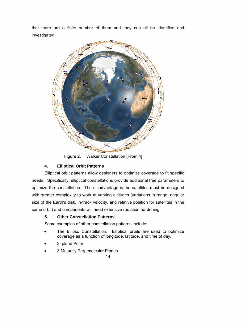
3. Walker Constellations Walker constellations are the most symmetric of the satellite patterns.

The Walker Delta Pattern contains a set number of satellites distributed evenly

within a set number of orbit planes at the same inclination. The ascending nodes

of the orbital planes are uniformly distributed around the equator and the

satellites are uniformly distributed within the orbital planes. Walker constellations

are completely symmetrical in longitude, but perhaps their greatest advantage is

14

that there are a finite number of them and they can all be identified and

investigated.

Figure 2. Walker Constellation [From 4]

4. Elliptical Orbit Patterns Elliptical orbit patterns allow designers to optimize coverage to fit specific

needs. Specifically, elliptical constellations provide additional free parameters to

optimize the constellation. The disadvantage is the satellites must be designed

with greater complexity to work at varying altitudes (variations in range, angular

size of the Earth's disk, in-track velocity, and relative position for satellites in the

same orbit) and components will need extensive radiation hardening.

5. Other Constellation Patterns Some examples of other constellation patterns include:

• The Ellipso Constellation. Elliptical orbits are used to optimize coverage as a function of longitude, latitude, and time of day.

• 2–plane Polar

• 3 Mutually Perpendicular Planes

15

• 2 Perpendicular Non-polar Planes

• 5-plane Polar "Streets of Coverage" E. SUMMARY

1. Process a. Establish Constellation-related mission requirements b. Do All Single Satellite Orbit Trades Except Coverage c. Do Trades Between Swath Width, Coverage, and

Number of Satellites d. Evaluate Ground Track Plots e. Adjust Inclination and In-plane Phasing f. Review the Rules of Constellation Design g. Document Reasons for Choices and Iterate

2. Design Factors a. Principal

(a) Number of Satellites

(b) Constellation Pattern

(c) Minimum Elevation Angle

(d) Altitude

(e) Number of Orbit Planes

(f) Collision Avoidance

b. Secondary (a) Inclination

(b) Between Plane Phasing

(c) Eccentricity

(d) Size of Stationkeeping Box [5]

16


17

II. GENETIC ALGORITHMS

A. THEORY Genetic algorithms (GA) use the concepts of natural selection and natural

genetics to solve optimization problems. Genetic algorithms use a population of

solutions to solve practical engineering optimization problems by estimating a

series of unknown parameters within a model of a physical system. [6]

B. HISTORY John Holland developed the concept of genetic algorithms at the

University of Michigan in the 1960s and 1970s. Holland's original intention was

to study the mechanisms of adaptation found in nature and to incorporate those

mechanisms into computer-simulated systems. Holland, with his students and

colleagues, developed a detailed approach to modeling natural evolution in the

form of computer algorithms. In 1975, Holland published his book, Adaptation in

Natural and Artificial Systems, in which he describes the basic approach to

population-based search characteristics. [7]

The research in genetic algorithms was mainly theoretical until the early

1980s. During this time, a large amount of work was done with fixed length

binary representation in function optimization. Specifically, Kenneth De Jong

attempted to capture the features of the adaptive mechanisms in the family of

genetic algorithms that constitute a robust search procedure. R. B. Hollstein

analyzed the effect that different selection and mating strategies have on the

performance of a genetic algorithm.

Throughout the 1980s, genetic algorithm applications were plentiful and

diverse. The genetic algorithm community routinely added insight into generality,

robustness and applicability of genetic algorithms. Each new insight contributed

to improving performance through tuning and specializing the genetic algorithm

operators. By the late 1980s, genetic algorithms were successfully applied to

optimization problems, scheduling, data fitting and clustering, trend spotting and

path finding. [8]

18

In 1989, David E. Goldberg published his book, Genetic Algorithms in

Search, Optimization, and Machine Learning. This book marked the second

major milestone in the history of genetic algorithms, accelerating the application

of genetic algorithms. Goldberg wrote about how genetic algorithms could be

used to solve a myriad of problems. He gives examples of researchers applying

genetic algorithms to solve various problems. Goldberg also presented the

theory of genetic algorithms, giving an unambiguous, succinct definition. Finally,

the Pascal source code Goldberg included allowed researchers to experiment

with genetic algorithms.

In 1991, Dave Davis further advanced the study of genetic algorithms

through his published book, The Handbook of Genetic Algorithms. Davis used

his book to teach the reader how to implement a genetic algorithm. Davis kept

the literature fundamental and did not include theoretical details. Davis also

included chapters outlining genetic algorithm applications written by researchers

who had successfully used genetic algorithms in their field. In 1991, The

Handbook of Genetic Algorithms contained the most current state of genetic

algorithm application and effectiveness. Davis successfully showed the utility of

a properly conceived genetic algorithm in advanced problem solving.

Unfortunately, it also showed the lack of industry participation as most of the

chapter authors were genetic algorithm specialists applying genetic algorithms to

a field of study and not necessarily field specialists using a genetic algorithm to

advance their research.

Interest and use of genetic algorithms has grown substantially since Davis'

book was published in 1991. Not only have there been multiple genetic algorithm

texts published in the last few years, but a well attended biannual international

conference met to discuss genetic algorithms. Additionally, genetic algorithm

usage increased dramatically as word of the many advantages and applications

spread as the volume of publications increased. Karr and Freeman wrote, "The

number of publications related to genetic algorithms is not growing, it has virtually

exploded over the last decade." [7]

19

C. PROCESS A genetic algorithm has five basic components:

1. A genetic representation of solutions to the problem

2. A way to create an initial population of solutions

3. An evaluation function rating solutions in terms of their fitness

4. Genetic operators that alter the genetic composition of children

during reproduction

5. Values for the parameters of genetic algorithms [9]

Typically, a genetic algorithm begins with an initial population of

individuals. The selection of the initial population is generally random and spread

throughout the search space. The individuals, representing a possible solution to

the problem, are evaluated based on defined wellness parameters and given a

score based on some measure of fitness. Generally, the individuals are

represented by binary encoding (strings) where bits are manipulated to create

new individuals.

Next, the genetic algorithm transforms using selection, crossover and

mutation. Selection alters the genetic algorithm through "picking" the best

individual to move on in the process. In selection, the poor performing samples

are discarded in favor of the better (fitter) performers. Thereby, the population

improves through natural selection similar to biological evolution.

Crossover allows two individuals to reproduce, creating offspring with

characteristics of each parent, similar to biological sexual reproduction.

Crossover hopes to capture the desired traits of each parent in the offspring

creating a fitter individual. One popular crossover method is to choose a

breaking point in the binary string and swap genetic information between each

individual before or after that point.

Mutation changes the characteristics of the individual without reproduction

with another. During mutation, bits are altered at random to produce an

individual with different characteristics. Through this process, some mutated

20

individuals will be fitter and some will be weaker. The fitter individuals are kept in

the population and the weaker individuals are discarded.

When selection, crossover and mutation are complete, a new population is

formed from a fresh generation of individuals. The genetic algorithm continues to

transform generation after generation, using selection, crossover and mutation,

until a set number of generations are met or a convergence point is reached.

[10] & [6]

D. APPLICATIONS Genetic algorithms have been used to solve a wide variety of problems.

Genetic algorithms are used primarily in the scientific and engineering industries

to solve complex mathematical problems. However, as exposure to the

advantages genetic algorithms present propagates, uses will become more

creative. Some example applications:

• Optimization. Genetic algorithms have been used in numerical optimization and combinatorial optimization problems.

• Automatic programming. Genetic algorithms have been used to evolve computer programs for specific tasks, and to design other computational methods.

• Machine learning. Genetic algorithms have been used to classify and predict tasks and to evolve aspects of particular machine learning systems.

• Economics. Genetic algorithms have been used to model processes of innovation. They have also been used in the development of bidding strategies and the emergence of economic markets.

• Immune systems. Genetic algorithms have been used to model somatic mutation during an individual's lifetime. Genetic algorithms have also been used in the discovery of multi-gene families during evolutionary time.

• Ecology. Genetic algorithms have been used to model biological arms races, host-parasite co-evolution, symbiosis, and resource flow.

• Population genetics. Genetic algorithms have been used in the study of population genetics.

21

• Evolution and learning. Genetic algorithms have been used to determine how individual learning and species evolution affect one another.

• Social systems. Genetic algorithms have been used to study the evolution of social behavior in insects and the evolution of cooperation and communication in multi-agent systems. [11]

• Image registration. Genetic algorithms have been used to generate three-dimensional visualizations of the human body, greatly increasing the scale of the search space.

• Recursive prediction of natural light levels. Genetic algorithms have been used to control artificial lights within buildings to act solely as a supplement to available daylight.

• Water network design. Genetic algorithms have been used as a design tool for water distribution network planning and management.

• Ground-state energy of the ±J spin glass. Genetic algorithms have been used to study spin glasses. Computational methods developed have been applied to questions in computer science, neurology and the theory of evolution.

• Liquid crystals. Genetic algorithms have been used in the estimation of the optical parameters of liquid crystals.

• Energy efficiency. Genetic algorithms have been used in the design of energy-efficient buildings.

• Human judgment. Genetic algorithms have been used as the fitness function of human judgment. The genetic algorithm converges at a useful rate and in the direction of improving subject preference. [1]

This list of applications is long but does not converge on the total number

of applications being considered. However, this list does illustrate the diversity of

genetic algorithms and gives a glimpse of future applications. The continued

success of genetic algorithms in the scientific and engineering communities will

pave the way for further experimentation across many disciplines.

E. VOCABULARY Some terms commonly used when Genetic Algorithms are referenced

include:

• Population – The set of individuals, items, or data from which a statistical sample is taken.

• Individuals – Separate and distinct from others of the same kind

22

• Search Space – The boundaries of the genetic algorithm

• Strings – Lines of binary code, analogous to chromosomes

• Selection – A natural or artificial process that favors or induces survival and perpetuation of one kind of organism over others that die or fail to produce offspring.

• Crossover – An exchange of genetic material between chromosomes.

• Mutation – A change of the DNA sequence within a gene or chromosome of an organism resulting in the creation of a new character or trait not found in the parental type.

• Fitness – The extent to which an organism is adapted to or able to produce offspring in a particular environment.

• Parent – An entity that produces or generates offspring

• Offspring – Something that comes into existence as a result

23

III. THE TRADITIONAL MODEL

A. BACKGROUND Most satellite constellations are designed using the traditional methods

(Walker, Streets of Coverage, etc.) described in Chapter I. This paper

investigates the performance achieved using GA techniques relative to these

traditional methods.

B. SPACE BASED RADAR (SBR) SBR offers sufficient complexity to strenuously test the two constellation

design methods for comparison.

1. Imaging radar The two main advantages of radar imaging over visual imaging sensors

are 24 hour capability (radar can "see" equally well in daylight and darkness) and

all weather capability (radar can "see" through clouds). Another advantage radar

has over other sensors is that radar can penetrate slightly beneath the surface of

the earth (mine detection capability).

a. Basics An SBR satellite moving through space in orbit sends microwave

radiation pulses through its antenna at the speed of light. The pulses are

directed in the range, look or across-track direction. Figure 1 illustrates the

following definitions:

• Slant Range – the line-of-site distance measured from the antenna to the target

• Ground Range – the horizontal distance measured along the surface from the ground track to the target

• Near Range – the area closest to the ground track at which a radar pulse intercepts the terrain

• Far Range – the area of pulse termination farthest from the ground track

• Depression Angle (β) – the angle measured from a horizontal plane downward to a specific part of the radar beam

• Look Angle (θ) – the angle measured from a vertical plane upward to a specific part of the radar beam

24

When measured to the same part of the beam, the depression angle and

the look angle are complementary angles (β + θ = 90°).

• Incidence Angle (φ) – the angle measured between the axis of the radar beam and a line perpendicular to the local ground surface that the beam strikes

• Grazing Angle (γ) – the complement of the incidence angle Consequently, the incidence angle and the grazing angle are a function of

both the illumination angle (β or θ) and the slope of the terrain. When the terrain

is horizontal, the depression and grazing angles are equal (β= γ) and the look

and incidence angles are equal (θ=φ).

• Resolution – the minimum separation between two objects of equal reflectivity that will enable them to appear individually in a processed radar image

• Pulse Rectangle – the surface area covered by the energy radiated from the sensor

When two or more objects fall within the same pulse rectangle they cannot

be resolved as separate entities. Rather, they are presented as one echo to the

radar system. If objects are separated by a distance exceeding the

corresponding dimension of the pulse rectangle, they will be imaged separately.

• Range Resolution – determines resolution cell size perpendicular to the ground track

• Azimuth Resolution – establishes the cell size parallel to the ground track

25

Figure 3. Definitions of Terms for Imaging Radar [From 12]

b. Detection Radar detection is defined as any object that reflects enough

energy to be distinguished from the background noise by the receiver (a blip on

the scope). Objects are categorized based on their ability to reflect microwave

radiation. Highly reflective objects create large radar signatures. Flat metal

surfaces produce large signatures; a significant portion of the microwave

radiation is reflected back to sensor. Objects with multiple surface angles

26

produce small signatures; most of the microwave radiation is reflected away from

the sensor.

c. Range Resolution Range resolution is determined by the length of the emitted

microwave pulse (pulse length). Pulse length is determined by multiplying the

pulse duration (τ) by the speed of light.

Two objects will appear as one unless all parts of their reflected

signals reach the radar sensor at different times. Consequently, objects must be

separated by a slant-range distance greater than one half of a pulse length to be

seen as separate entities.

Ground range resolution is half the pulse length divided by the

cosine of the depression angle. Therefore, ground range resolution can be

improved by increasing the distance from the ground track and by shortening the

pulse length.

d. Signal Shape Target resolution is determined based on the pulse length (“t” in the

figure below). Related to pulse length, pulse repetition interval (PRI, “T” in the

figure below) is the interval between pulses. As illustrated, the PRI duration is

generally much longer than the pulse length. The pulse repetition frequency

(PRF) is the inverse of the PRI.

Figure 4. Radar Pulse [From 13]

27

Pulse length is also related to spectrum. Range resolution is

proportional to the length of the pulse. Essentially, a short pulse length contains

a wide spectrum and a long pulse length is restricted to a narrow spectrum.

One solution to the pulse vs. spectrum conundrum is using

frequency differential. By modulating the frequency of the pulses and monitoring

the frequencies of the returns, the two objects can be discerned even if they

overlap in time.

e. Azimuth Resolution Beam width is determined by antenna size and wavelength.

Azimuth, or along-track, resolution is a function of the beam width. The beam

width increases with range, therefore the greater the range the poorer the

azimuth resolution. Two objects at the same range within the beam will appear

as one because their returns will be received at the same time. Therefore, to

distinguish between two objects, their ground separation distance in azimuth

must be greater than the width of the radar beam.

f. Resolution Azimuth resolution is the slant range multiplied by the wavelength

divided by the length of the antenna. Therefore, azimuth resolution improves as

range decreases, antenna length increases and wavelength decreases. To

improve azimuth resolution, use a long antenna, a short operating wavelength, a

close-in interval, or a combination of these factors. The problems are antenna

size is limited and the all weather capability of radar is reduced when wavelength

is less than 3 cm. The solution is Synthetic Aperture Radar (SAR).

2. Synthetic Aperture Radar (SAR) SAR uses the motion of the emitting vehicle (the satellite) to increase the

length of the effective antenna. The SAR vehicle carries a relatively short

antenna and intercepts the emitted signal at different paths along the flight as

shown in Figure 5.

28

Figure 5. SAR Effective Antenna Length [From 12]

The longer resulting antenna is simulated by using the coherence of radar

signals. The main beam footprint is then twice the altitude of the sensor

multiplied by the wavelength and divided by the antenna length. The array

footprint on the ground is half the length of the antenna.

SAR sensors generally have two modes of operation: scan and spotlight.

In scan mode, the SAR antenna is pointed in a fixed direction; the only motion is

the motion of its platform (aircraft or satellite). Scan mode allows imaging of a

large area with fixed resolution. In spotlight mode, the SAR antenna is

articulated to continuously point at a specific location or target. Spotlight mode

restricts the area of an image, but provides greater resolution.

The resolution of an object is proportional to the time it is in the radar

beam. That period of time increases with range and therefore azimuthal

resolution is range independent for scan mode. The along-track, linear resolution

increases (gets worse) with range since the beam has a fixed angular extent.

However, this is compensated for by the fact that as the beam diverges with

increasing range, any target at a more distant slant range spends more time in

the beam. The net effect is a fixed, “range independent” resolution.

In spotlight mode, antenna length is arbitrarily large because the interval

at which radar energy is returned from the target is determined by the operator.

As R. C. Olsen points out in reference 10:

29

In processing, the azimuth details are determined by establishing the position-dependent frequency changes or shifts in the echoes that are caused by the relative motion between terrain objects and the platform. To do this, a SAR system must unravel the complex echo history for a ground feature from each of a multitude of antenna positions.

For example, if we isolate a single ground feature, the following frequency modulations occur as a consequence of the forward motion of the platform:

Positive Doppler - the feature enters the beam ahead of the platform and its echoes are shifted to higher frequencies

Zero Doppler – the platform is perpendicular to the features position and there is no shift in frequency

Negative Doppler - the platform moves away from the feature, the echoes have lower frequencies than the transmitted signal.

The Doppler shift information is then obtained by electronically comparing the reflected signals from a given feature with a reference signal that incorporates the same frequency of the transmitted pulse. The output is known as a phase history, and it contains a record of the Doppler frequency changes plus the amplitude of the returns from each ground feature as it passed through the beam of the moving antenna. [12]

3. Ground Moving Target Indicator (GMTI) In contrast to SAR imaging, GMTI detects the Doppler shift in frequency

caused when the radar pulse is reflected by a moving object. This Doppler shift

enables a GMTI sensor to rapidly distinguish between a moving object and the

stationary background. GMTI is able to distinguish moving targets from water

and surface clutter over large areas in all weather and in darkness.

30

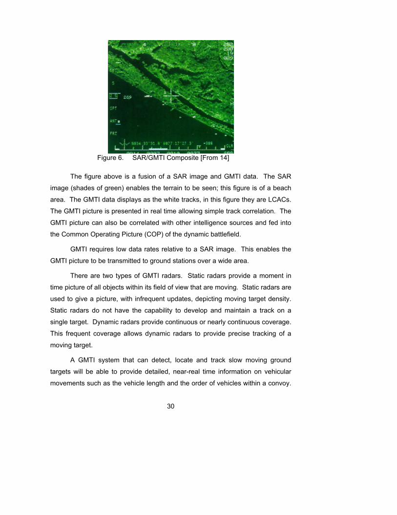
Figure 6. SAR/GMTI Composite [From 14]

The figure above is a fusion of a SAR image and GMTI data. The SAR

image (shades of green) enables the terrain to be seen; this figure is of a beach

area. The GMTI data displays as the white tracks, in this figure they are LCACs.

The GMTI picture is presented in real time allowing simple track correlation. The

GMTI picture can also be correlated with other intelligence sources and fed into

the Common Operating Picture (COP) of the dynamic battlefield.

GMTI requires low data rates relative to a SAR image. This enables the

GMTI picture to be transmitted to ground stations over a wide area.

There are two types of GMTI radars. Static radars provide a moment in

time picture of all objects within its field of view that are moving. Static radars are

used to give a picture, with infrequent updates, depicting moving target density.

Static radars do not have the capability to develop and maintain a track on a

single target. Dynamic radars provide continuous or nearly continuous coverage.

This frequent coverage allows dynamic radars to provide precise tracking of a

moving target.

A GMTI system that can detect, locate and track slow moving ground

targets will be able to provide detailed, near-real time information on vehicular

movements such as the vehicle length and the order of vehicles within a convoy.

31

To do this, a GMTI system must be able to generate and maintain numerous

tracks automatically using the following metrics as listed in reference [15]:

• Probability of Detection – the probability of detecting a given target at a given range any time the radar beam scans across it

• Target Location Accuracy – a function of platform self-location performance, radar pointing accuracy, azimuth resolution, and range resolution

• Minimum Detectable Velocity – the rate of movement determining whether the majority of military traffic will be detected

• Target Range Resolution – the fidelity determining whether two or more targets moving in close proximity will be detected as individual targets

• Stand-off Distance – the distance separating a radar system from the area it is covering

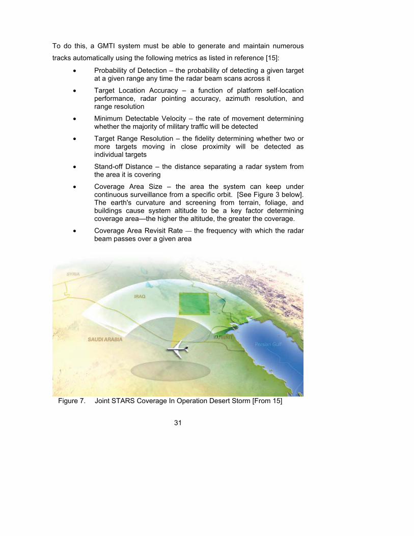
• Coverage Area Size – the area the system can keep under continuous surveillance from a specific orbit. [See Figure 3 below]. The earth's curvature and screening from terrain, foliage, and buildings cause system altitude to be a key factor determining coverage area—the higher the altitude, the greater the coverage.

• Coverage Area Revisit Rate — the frequency with which the radar beam passes over a given area

Figure 7. Joint STARS Coverage In Operation Desert Storm [From 15]

32

The accuracy of the GMTI picture is dependent on the system's

performance in these matrices. Poor performance can lead to inaccuracies in

both location and timeframe of the targets position. Precise positioning of slow

moving vehicles is crucial for targeting. The advantage of using radar is the

system can often counter the effects of enemy camouflage, concealment and

deception.

Most GMTI systems can collect SAR and GMTI information (but usually

not both at the same time). Using SAR still images with GMTI can be valuable in

ascertaining whether a target has stopped moving or has been lost. Using GMTI

and high-resolution SAR pictures allow target characterization by Automatic

Target Recognition (ATR) algorithms. [15]

4. Future The Air Force is the executive agent for space. As such they are tasked

with providing an effective cross service SBR system.

Ideally, the new arrangement will amalgamate all SBR requirements into

one SAR/GMTI capable system with the next decade. The SBR system goal will

be to provide integrated data without the user knowing the source. The new

program was to provide initial SBR capability by 2010.

a. The Requirements Dilemma The challenge with any system is to integrate all service's

requirements into one efficient design. The primary challenge is determining how

the system's information will get to the battlefield commanders (an arguing point

that has led to the demise of systems in the past). Another challenge is

determining whether the SBR constellation will be flown in LEO (better

operational access for GMTI but requires more hand-offs) or MEO (simultaneous

target access by two satellites but long SAR integration times).

Several technologies have advanced since initial plans for a SBR

constellation were scrapped, including active electronically scanned arrays and

synthetic aperture radar.

33

b. From Scratch The SBR constellation will be developed from the ground up. This

means the constellation will be developed without using a past or existing

constellation as a model. The SBR system was designated by Martin R.

Sambur, Air Force acquisition chief, a "pathfinder" program; employing new,

innovative and streamlined acquisition strategies. The SBR system is required to

use the spiral development acquisition strategy, making incremental

improvements to the system during development. The SBR will also be the first

program developed under the pan-agency space hardware acquisition system.

SBR most likely will consist of 20 to 25 light, inexpensive satellites

in LEO, MEO or a LEO/MEO orbit. The physical characteristics are still in the

early stages of development. [16]

b. Reality As 18 June 2004, the 108th Congress met and again all but

cancelled the SBR program. The DoD Appropriations Committee directed the Air

Force to fundamentally restructure the program. Some Committee findings are

below:

The Air Force requested $327,732,000 for the Space Based Radar program. The Committee recommends $75,000,000, a reduction of $252,732,000, and directs that the Air Force fundamentally restructure the program to meet the concerns addressed below.

The Space Based Radar (SBR) program is intended to provide near continuous, global radar imagery and surface moving target indication (SMTI) as well as high resolution terrain information. Advocates describe the program as a key contributor to achieving `global persistent surveillance'. Though the pursuit of persistent surveillance is a noble goal, the Committee believes the Space Based Radar program as currently structured:

--Is neither affordable nor likely to produce the results claimed by its advocates, within any reasonable definition of cost, technical challenge, or risk.

--Would consume a disproportionate share of resources from within an already highly stressed DoD space and surveillance budget;

34

--And finally, is simply a less-pressing priority than many other near-and mid-term needs confronting the Department of Defense.

Committee Views and Recommendations- In summary, in and of itself the SBR development program is fraught with enough uncertainties to call into question its viability. Indeed, even under the Administration's own plans the SBR program of record is underfunded in the current Future Year Defense Program by $2 billion, a shortfall resulting from the Department's unwillingness to fully fund this program. The Committee sees little prospect of this changing in light of the other fiscal challenges confronting the Department. These include the well-documented `procurement bow-wave'; this Administration's emphasis on missile defense and other transformational programs; and now, and most importantly, the as-yet-unbudgeted future manpower, operational, and equipment recapitalization requirements stemming from operations in Iraq and the Global War on Terrorism. The Committee concludes that against these demands, SBR simply cannot be afforded budget priority.

Without a new approach, the Committee sees little future for the Space Based Radar program. Accordingly, the Committee recommends $75,000,000, a reduction to the request of $252,732,000. These funds are provided to redirect the Air Force's development efforts towards technologies and concepts that would lead to program costs far lower than currently conceived. The focus should be on seeking breakthroughs that fundamentally change the cost-benefit equation for a space based radar system. [17]

C. DISCOVERER II Discoverer II was chosen as a model for comparison because the

Discoverer II system was the most complete SBR design.

The Discoverer II Joint Program was a joint venture between the National

Reconnaissance Office (NRO), Defense Research Projects Agency (DARPA)

and the U.S. Air Force. Discoverer II was designed to provide high-range

resolution ground moving target indication (HRR-GMTI), synthetic aperture radar

(SAR) imaging and high resolution digital terrain mapping data collection

capabilities. The system was designed to allow joint task force commanders the

ability to task the assets and receive data via downlink directly to theater ground

stations.

35

1. Background Discoverer II was to be a pioneer in the ability to detect and track moving

targets on the earth's surface from space. Additionally, Discoverer II was

designed to produce high-resolution imagery and collect precision Digital Terrain

Elevation Data (DTED).

A successful Discoverer II program would have revolutionized the

coverage and timeliness of ISR under the direct control of commanders.

Additionally, a goal of the Discoverer II program was to demonstrate the ability to

populate a constellation with satellites for under $100 million, and to reduce the

20 year life-cycle cost to less than $10 billion.

2. Capabilities The Discoverer II program strived to improve the reconnaissance and

surveillance support provided to the theater commanders. To this end, the

Discoverer II engineers sought SBR capabilities that would complement,

enhance and improve on the existing capabilities airborne assets, such as Joint

Surveillance Target Attack Radar System (JSTARS), U-2s and unmanned aerial

vehicles (UAVs), provide. With Discoverer II assistance, leaders envisioned

providing U.S theater commanders the "information superiority" necessary to

employ the smaller, lighter, highly mobile and often widely dispersed joint forces

of the future.

The Discoverer II would have been capable of the following:

• Assured, on-demand reconnaissance of areas of interest worldwide during peacetime, periods of heightened tension, hostilities and operations other than war.

• Near-continuous surveillance of selected ground and maritime objects.

• Coverage of blind spots, or “shadowed” areas, obscured from view of standoff airborne platforms.

• Rapid acquisition and tracking of mobile, time-critical targets throughout the depth of the theater.

• Precise geolocation of objects to support munitions targeting.

• High-quality terrain mapping.

36

To accomplish these goals, the Discoverer II program would have required

a large constellation with a large number of inexpensive satellites with the

following capabilities:

• Day/night, all-weather, near-continuous, global GMTI search/track, and high resolution imagery,

• Theater dynamic tasking of space-based, or “overhead,” GMTI and imagery collection,

• Near-real-time, direct downlink to theater of overhead GMTI and imagery collection; and,

• Collection of precision Digital Terrain Elevation Data (DTED). Additional requirements, and costs, would have been in-theater

infrastructure and additional manning as well as the ability to use the same

tactical ground stations used by airborne collectors.

3. General Characteristics • Function: HRR-GMTI, HR-SAR, HR digital mapping data collection

• Constellation Size: 24 satellites

• Power: Solar panels

• Launch Vehicle: MLV or HLV (2+ per launch vehicle)

• Mass: 1500 kg

• Frequency: X band (10 GHz)

• Antenna Type: 2D, electronically scanned array (ESA)

• Antenna Dimension: 40 m2

• Altitude: 770 km

• Design Life: 10 years

• In-Theater C2: Dynamic, on-demand collection tasking; near real-time, direct downlink of mission data

• Theater Ground Station: Common Imagery Ground/Surface Station (CIG/SS) compliant

• In-Theater Communications: Modified CDL (548 Mbps)

• Reach-Back CONUS Communications: Relay and/or satellite cross-links [18]

37

4. Reality From House Rpt.106-644 - DEPARTMENT OF DEFENSE

APPROPRIATIONS BILL, 2001:

The Air Force, Defense Advanced Research Projects Agency, and the National Reconnaissance Office collectively requested $130,000,000 for the Discoverer II satellite technology demonstration program. The Committee recommends no funding, a decrease of $130,000,000. The fiscal year 2000 Defense Appropriations Act provided sufficient funding for the Discoverer II program to conclude the phase I studies and analysis portion of the program along with related risk reduction efforts. With phase I now funded to completion, the Committee recommends that the Discoverer II program be terminated.

The Committee makes this recommendation for the following reasons: (1) Discoverer II has no documented requirement or concept of operations; (2) the cost of the engineering and manufacturing development phase of the program, which the program office estimates at $702 million and which will in all likelihood exceed $1 billion, is of a magnitude ordinarily associated with the development of fully operational satellites and therefore unaffordable given the limited operational benefits of a technology demonstration program; (3) the Department has conducted no trade-off analysis between Discoverer II and other systems and processes that could deliver ground moving target indication data to warfighters; and, (4) the Department has failed to analyze the impact a Discoverer II constellation would have on an already overtaxed imagery processing, exploitation and dissemination system.

Even if successful, there is no guarantee the Air Force could ever build, launch, operate and maintain a Discoverer II constellation without a substantial top line increase to its budget. By some estimates the cost of a fully functional Discoverer II constellation could reach $25 billion. In the face of other severe shortfalls in space and aircraft modernization the Committee concludes that Discoverer II is of low priority and recommends its termination.

The Committee discusses its recommendation more fully in the classified annex to this report. [19]

38

D. THE MODEL The Discoverer II constellation was modeled using Satellite Tool Kit for

demonstration and comparison with the Genetic Algorithm constellation. The

following proposed Discoverer II system parameters were used:

• Total Satellites: 24

• Number of Planes: 8

• Satellites/Plane: 3

• Type of Orbit: Walker

• Inclination: 53°

• Altitude: 770 km

• Latitude Coverage: 65°N to 65°S

• Grazing Angle: 12°

• Slope Angle: 70°

• Cone Angle: 45°

• Response Time: 90%/15 min* *90% of imaging requests result in collection within 15 minutes

• Modes: National Image Interpretability Rating Scale (NIIRS)-3 (3 meter/360,000 km2/hr)

NIIRS-5 (1 meter/27,000 km2/hr)

(NIIRS-7) Point/Spot (.3 meter/4 km2, 60/hr)

MTI (3 meter/360,000 km2/hr)

Collection Rates:

• HR-GMTI: Minimum Detectable Velocity (MDV) = 4 kph Maximum Velocity = 100 kph

2,000,000 km2/hr (600 km2/sec)

• STRIP SAR/GMTI: 3 meter impulse response (IPR) imagery 700,000 km2/hr

• SCAN SAR: 1 meter IPR 100,000 km2/hr

• SPOT SAR: 0.3 meter IPR

39

IV. THE GENETIC ALGORITHM

Chapter II examined the fundamentals of genetic algorithms. This chapter

will focus on the specific implementation used for this thesis. First, some of the

concepts presented earlier will be reviewed and expanded in light of the

developed application. Following that, the major modules of the program will be

examined with an example to illustrate how the genetic algorithm operates. A

discussion of the interface with Satellite Tool Kit (STK) will follow. Finally, the

chapter will conclude by suggesting follow-on research in implementing a genetic

algorithm for constellation design.

A. BACKGROUND A genetic algorithm is a search tool that leverages biologic, genetic, and

evolutionary processes. Although each implementation of a genetic algorithm

models biologic processes, the granularity of the model varies widely. Most

implementations use binary encoding, in which the variables optimized are

represented as binary strings. Other encoding methods are available, including

Gray encoding and whole number encoding. Our main objective was to test the

usefulness of genetic algorithms as a constellation design tool, binary encoding

was chosen for the simplicity of implementation.

Most biological organisms, including all animals, are diploid, having paired

chromosomes. In the process of reproduction, the offspring receives one

chromosome of the pair from the mother and the other from the father. Typically,

genetic algorithms are haploid, having only single chromosomes. Reproduction

is the result of crossover between the mother’s and father’s chromosomes.

Genetic algorithms are rarely constructed to be diploid, because it requires the

user to handle the genetic concept of dominance. In biologic genetics, a

dominant gene is expressed in the heterozygous or homozygous instance; in

other words, if it is present in either or both of the paired chromosomes. The

recessive gene is only expressed in the homozygous instance. Dominance

enables greater genetic diversity to be maintained in a population, because it is

possible for the recessive gene to be passed on to future generations without

40

having it expressed. This leads us into a quick explanation of genotype and

phenotype. Genotype is the sum total of the genetic material present in an

organism; all of the possible genes that could be passed on to offspring.

Phenotype is the expressed or visible manifestation of an individual’s genotype.

A non-haploid genetic algorithm would more closely model biologic genetic

processes and provide greater genetic diversity. However, how can you model a

diploid organism in a binary encoded genetic algorithm and resolve the

dominance problem? Which instance, zero (0) or one (1), should be dominant in

the calculation of the phenotype? The solution arrived at elegantly achieves

increased genetic diversity without creating a dominance problem: triploid

chromosomes. By using a three-chromosome genotype, the individuals have

greater genetic diversity and the phenotype is calculated by the instance, zero (0)

or one (1), in the majority in the genotype chromosomes. The problem with

triploid individuals is: how do you get three chromosomes from two parents? The

simple answer is you don’t; you have three parents. Therefore, the genetic

algorithm would use binary encoding and a phenotype derived from a triploid

chromosome genotype.

The final decision was how many chromosome triplets should be used to

represent a constellation. It was a choice between using long chromosomes to

represent an entire constellation, medium length chromosomes to represent each

satellite in a constellation, or short chromosomes representing each orbital

element of each satellite in a constellation. Also implicit in this step was deciding

what dynamic range was required for each orbital element; this would affect the

length of the chromosomes. Here, the programming language, Visual Basic,

helped narrow the decision. Visual Basic supports bit-wise comparisons of

numeric data types. The bit-wise comparison operators are used to calculating

the phenotype from the triploid genotype and to effect crossover and mutation.

Three integer data types in Visual Basic supported bit-wise comparisons. The

long data type is a 32-bit number and can represent integer values from -

2,147,483,648 to 2,147,483,648. The second data type is integer. It is a 16-bit

number, representing values from –32,768 to 32,767. The final data type is byte,

41

8-bits long and represents values from 0 to 255. The first two data types were

deemed too granular in this application. For example, with the integer data type,

if the possible range of inclinations is 0 to 180 degrees, each step of the data

represents a change in inclination of 0.00274658203125 degrees. Such a small

difference cannot significantly affect a difference in the performance of a

constellation and most certainly cannot be achieved or maintained by a satellite

in orbit. Therefore, all of the orbital elements were represented by the byte data

type, which equates to an 8-bit binary string.

Of the six classical orbital elements, only four needed to be represented.

Synthetic Aperture Radar requires the altitude to remain relatively constant. For

this reason, all of the orbits evaluated had an eccentricity of zero. With an

eccentricity of zero, the argument of perigee no longer has meaning. Of the four

remaining orbital elements, the altitude and inclination of all satellites in a

constellation would be equal, but could vary between constellations. This

limitation was placed on the search space to guarantee that the constellation

would remain constant over time with no differential node rotation, to enable data

fusion, and to ensure the constellation could be populated with identical

satellites.

B. THE GENETIC ALGORITHM Now that we understand what orbital elements are represented and how

they are encoded, an 8-bit phenotype for each orbital element of each satellite

derived from an 8-bit triploid genotype, let us examine the genetic algorithm itself.

First, an overview of the basic flow of the genetic algorithm will be presented. A

more detailed explanation of the major sub routines with a simplified example will

be presented. The simplified example will help to illustrate the major concepts.

The entire genetic algorithm code is included as Appendix A.

1. Overview As presented before, every genetic algorithm has certain characteristics:

an data encoding scheme; an initial population of individuals; a method for

evaluating the fitness of the individuals; use of genetic operators (crossover,

mutation, selection); a means of creating offspring; an iterative loop that

42

continues until the termination criteria is met. The application of these basic

characteristics is what differentiates one genetic algorithm from another. The

figure below illustrates the main execution loop of the genetic algorithm used in

this study.

Mating Coupler

Update Fitness Array

Crossover

Mutation Engine

Evaluate Fitness

Crossover Engine

Create Initial Population

Mutation

Create Offspring

Scale Fitness

Calculate Phenotype

Figure 8. Genetic Algorithm Pseudocode

2. Create Initial Population The genetic algorithm first must create a starting population. In all trials

conducted as part of this study the initial population size was twelve

constellations. The initial population was created by assigning a randomly

generated 8-bit value to each genotype chromosome. This was repeated for

each orbital element of each satellite in the constellation. In the example, a three

individual population will be created. Each individual in the example will consist

of 4-bit triploid chromosomes. The following three individuals were created by

using a standard 25-cent random binary number generator.

Individual A B C Genotype 1 0100 1001 0111 Genotype 2 0011 0111 1110 Genotype 3 1011 1101 1101 3. Calculate Phenotype

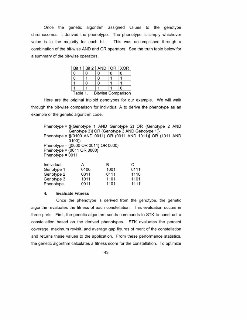
43

Once the genetic algorithm assigned values to the genotype

chromosomes, it derived the phenotype. The phenotype is simply whichever

value is in the majority for each bit. This was accomplished through a

combination of the bit-wise AND and OR operators. See the truth table below for

a summary of the bit-wise operators.

Bit 1 Bit 2 AND OR XOR0 0 0 0 0 0 1 0 1 1 1 0 0 1 1 1 1 1 1 0 Table 1. Bitwise Comparison

Here are the original triploid genotypes for our example. We will walk

through the bit-wise comparison for individual A to derive the phenotype as an

example of the genetic algorithm code.

Phenotype = [(Genotype 1 AND Genotype 2) OR (Genotype 2 AND

Genotype 3)] OR (Genotype 3 AND Genotype 1) Phenotype = [(0100 AND 0011) OR (0011 AND 1011)] OR (1011 AND

0100) Phenotype = [0000 OR 0011 OR 0000 Phenotype = 0011 OR 0000 Phenotype = 0011 Individual A B C Genotype 1 0100 1001 0111 Genotype 2 0011 0111 1110 Genotype 3 1011 1101 1101 Phenotype 0011 1101 1111 4. Evaluate Fitness Once the phenotype is derived from the genotype, the genetic

algorithm evaluates the fitness of each constellation. This evaluation occurs in

three parts. First, the genetic algorithm sends commands to STK to construct a

constellation based on the derived phenotypes. STK evaluates the percent

coverage, maximum revisit, and average gap figures of merit of the constellation

and returns these values to the application. From these performance statistics,

the genetic algorithm calculates a fitness score for the constellation. To optimize

44

the performance of the constellation, we desire to minimize the maximum revisit

and average gap time and maximize the percent coverage. To drive the fitness

score to a meaningful value, it was necessary to subtract the coverage

percentage from one. This enabled the genetic algorithm to converge toward an

optimal solution by minimizing the fitness score. In our trivial example to parallel

the genetic algorithm, the fitness will be the number of ones in the phenotype,

optimizing to a minimum.

Individual A B C Genotype 1 0100 1001 0111 Genotype 2 0011 0111 1110 Genotype 3 1011 1101 1101 Phenotype 0011 1101 1111 Fitness 2 3 4 5. Scale Fitness In the first generation, the fitness scores are stored in an array from lowest

score to highest, best fitness to worst. In every other generation, the fitness is

compared to the stored scores and, if lower, is stored. All other scores cascade

down one position and the worst score drops off. Once the entire generation has

been evaluated against the best fitness scores, the array is scaled in preparation

for the roulette wheel selection of parents. The process requires each fitness

score to be weighted, normalized and finally scaled. Let us walk through this

process with our example.

Individual A B C Genotype 1 0100 1001 0111 Genotype 2 0011 0111 1110 Genotype 3 1011 1101 1101 Phenotype 0011 1101 1111 Fitness 2 3 4 Weighted Fitness 4.5 3 2.25 Normalized Fitness 0.46 0.31 0.23 Scaled Fitness 0.46 0.77 1 Weighted Fitness = Fitness Summation / Individual Fitness Normalized Fitness = Weighted Fitness / Weighted Fitness Summation Scaled Fitness = Normalized Fitness + Previous Scaled Fitness

45

6. Crossover Engine and Crossover The final step prior to selecting parents and generating the next

generation of offspring is crossover. In haploid genetic algorithms, the process of

crossover is used to create offspring. However, in this triploid genetic algorithm,

crossover is an operation that occurs between genotype chromosomes of an

individual. Each 8-bit chromosome has seven possible crossover loci. The

algorithm generates a random number and compares this to the crossover

probability for each crossover locus. If the random number is less than the

crossover probability, crossover occurs at that locus between that chromosome

and one of the other two. To ensure that crossover can take place between any

and all of the genotype chromosomes, the genetic algorithm cycles through the

genotypes. A crossover indicated in the first genotype occurs between

chromosomes one and two; in the second genotype, the crossover occurs

between the chromosomes two and three; and in the third genotype, the

crossover occurs between chromosomes three and one. Because the orbital

parameters of the constellations evaluated by STK are based on the phenotype,

crossover has no effect on the fitness of a constellation. It does not change the

derived phenotype because it does not change the overall majority of bits; rather

it only changes the genotype chromosomes. Although crossover has no effect

on the constellations fitness, it does affect the offspring it creates. By changing

the genotype chromosomes, crossover affects the genotype string passed from

parent to child. This enables a parent that displays one trait to pass the genetic

material for another trait onto its child. The constellations that have the highest

fitness are subject to crossover every generation. This enables a greater genetic

diversity in the possible offspring. Genetic diversity is the single greatest

protection against early convergence to a local optimum before thoroughly

exploring the search space. The process of crossover is accomplished through

bit-wise comparisons. A crossover mask is generated which effectively splits the

two genotypes at the crossover locus. The tails are then switched between the

genotypes and are then rejoined to the head to form two new genotype

chromosomes. In our trivial example, we will set the crossover probability at 0.5.

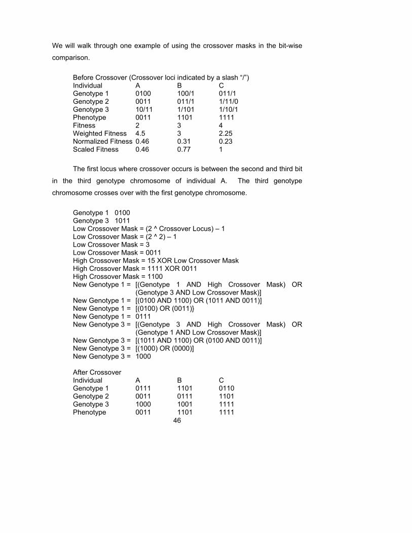
46

We will walk through one example of using the crossover masks in the bit-wise

comparison.

Before Crossover (Crossover loci indicated by a slash “/”) Individual A B C Genotype 1 0100 100/1 011/1 Genotype 2 0011 011/1 1/11/0 Genotype 3 10/11 1/101 1/10/1 Phenotype 0011 1101 1111 Fitness 2 3 4 Weighted Fitness 4.5 3 2.25 Normalized Fitness 0.46 0.31 0.23 Scaled Fitness 0.46 0.77 1 The first locus where crossover occurs is between the second and third bit

in the third genotype chromosome of individual A. The third genotype

chromosome crosses over with the first genotype chromosome.

Genotype 1 0100 Genotype 3 1011 Low Crossover Mask = (2 ^ Crossover Locus) – 1 Low Crossover Mask = (2 ^ 2) – 1 Low Crossover Mask = 3 Low Crossover Mask = 0011 High Crossover Mask = 15 XOR Low Crossover Mask High Crossover Mask = 1111 XOR 0011 High Crossover Mask = 1100 New Genotype 1 = [(Genotype 1 AND High Crossover Mask) OR

(Genotype 3 AND Low Crossover Mask)] New Genotype 1 = [(0100 AND 1100) OR (1011 AND 0011)] New Genotype 1 = [(0100) OR (0011) New Genotype 1 = 0111 New Genotype 3 = [(Genotype 3 AND High Crossover Mask) OR

(Genotype 1 AND Low Crossover Mask)] New Genotype 3 = [(1011 AND 1100) OR (0100 AND 0011)] New Genotype 3 = [(1000) OR (0000)] New Genotype 3 = 1000 After Crossover Individual A B C Genotype 1 0111 1101 0110 Genotype 2 0011 0111 1101 Genotype 3 1000 1001 1111 Phenotype 0011 1101 1111

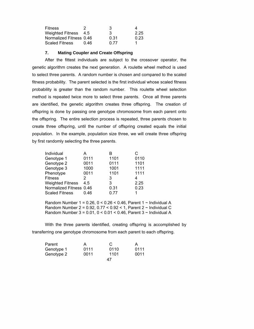
47

Fitness 2 3 4 Weighted Fitness 4.5 3 2.25 Normalized Fitness 0.46 0.31 0.23 Scaled Fitness 0.46 0.77 1 7. Mating Coupler and Create Offspring After the fittest individuals are subject to the crossover operator, the

genetic algorithm creates the next generation. A roulette wheel method is used

to select three parents. A random number is chosen and compared to the scaled

fitness probability. The parent selected is the first individual whose scaled fitness

probability is greater than the random number. This roulette wheel selection

method is repeated twice more to select three parents. Once all three parents

are identified, the genetic algorithm creates three offspring. The creation of

offspring is done by passing one genotype chromosome from each parent onto

the offspring. The entire selection process is repeated, three parents chosen to

create three offspring, until the number of offspring created equals the initial

population. In the example, population size three, we will create three offspring

by first randomly selecting the three parents.

Individual A B C Genotype 1 0111 1101 0110 Genotype 2 0011 0111 1101 Genotype 3 1000 1001 1111 Phenotype 0011 1101 1111 Fitness 2 3 4 Weighted Fitness 4.5 3 2.25 Normalized Fitness 0.46 0.31 0.23 Scaled Fitness 0.46 0.77 1 Random Number 1 = 0.26, 0 < 0.26 < 0.46, Parent 1 ~ Individual A Random Number 2 = 0.92, 0.77 < 0.92 < 1, Parent 2 ~ Individual C Random Number 3 = 0.01, 0 < 0.01 < 0.46, Parent 3 ~ Individual A With the three parents identified, creating offspring is accomplished by

transferring one genotype chromosome from each parent to each offspring.

Parent A C A Genotype 1 0111 0110 0111 Genotype 2 0011 1101 0011

48

Genotype 3 1000 1111 1000 Offspring D E F Genotype 1 0111 0110 0111 Genotype 2 1101 0011 0011 Genotype 3 1000 1000 1111 8. Mutation Engine and Mutation From the example one can see there is no mechanism in the genetic

algorithm that requires all or any of the parents to be different. It is possible for

all three parents to be the same individual. This does not mean that the offspring

will be identical to the parent or each other; the mutation operation allows the

offspring to vary from the parent. Again, because crossover occurs only within

the genotype of an individual, it has no effect on the individual’s fitness, and it is

unnecessary to re-evaluate the fitness of an individual. The only processes that

require an individual’s fitness to be evaluated are creation and mutation. For this

reason, mutation directly follows the creation of offspring. In order to make the

genetic algorithm efficient, once an individual’s fitness is calculated, the individual

is not permitted to mutate. Mutation is simply a bit flip.

The mutation operation is similar to the crossover operation in its

implementation. A random number is compared to the mutation probability to

determine if mutation occurs. If mutation occurs the program generates a

mutation mask which is then bit-wise compared to the genotype chromosome to

cause the mutation. The major difference is that crossover occurs at the loci

between the bits whereas mutation affects the bits themselves. A reasonable

starting value for the mutation probability is one over the chromosome length.

With that in mind, the mutation probability for our example will be 0.25.

Before Mutation (bits to be mutated indicated with [ ]) Offspring D E F Genotype 1 0111 01[1]0 0111 Genotype 2 1101 0011 [0]0[1]1 Genotype 3 1[0]00 1000 1111

49

The first instance of mutation occurs in the third genotype chromosome of

Offspring D at the third bit from the right. The following illustrates the bitwise

comparison used to cause the mutation.

Mutation Mask = 2 ^ (Mutation Bit -1) Mutation Mask = 2 ^ (3 – 1) Mutation Mask = 2 ^ 2 Mutation Mask = 4 Mutation Mask = 0100 Genotype 3(after mutation) = Genotype 3(before mutation) XOR Mutation Mask Genotype 3(after mutation) = 1000 XOR 0100 Genotype 3(after mutation) = 1100 After Mutation Offspring D E F Genotype 1 0111 0100 0111 Genotype 2 1101 0011 1001 Genotype 3 1100 1000 1111 9. Finishing the Example The genetic algorithm is now at a point where it increments the generation

counter by one and loops back to the phenotype calculator. To finish the simple

example presented let us calculate the phenotype and fitness of the offspring.

Individual A B C Genotype 1 0111 1101 0110 Genotype 2 0011 0111 1101 Genotype 3 1000 1001 1111 Phenotype 0011 1101 1111 Fitness 2 3 4 Weighted Fitness 4.5 3 2.25 Normalized Fitness 0.46 0.31 0.23 Scaled Fitness 0.46 0.77 1 Offspring D E F Genotype 1 0111 0100 0111 Genotype 2 1101 0011 1001 Genotype 3 1100 1000 1111 Phenotype 1101 0000 1111 Fitness 3 0 4

50

In this simplified example, the genetic algorithm was able to find the

optimum solution in just two generations. Typically, the optimum solution is

unknown, and the genetic algorithm must be given some other termination

criteria.

C. PARAMETERS A genetic algorithm has certain parameters which must be set by the

experimenter. In this application the parameters were: crossover probability,

mutation probability, population size, and number of generations.

1. Population Size and Number of Generations One problem that remains unresolved directly impacts the population size

and the number of generations. The genetic algorithm establishes a socket

TCP/IP connection with STK which it uses to send constellations to be evaluated

and receives data in return. The problem is that the STK application overruns

the virtual memory of the computer after evaluating about 30 generations. This

causes the genetic algorithm to lock up. In order to generate the data for this

thesis a workaround was developed. The genetic algorithm would have the

option of either generating a random initial population or reading an initial

population in from a data file. The algorithm ran for 20 generations and the fittest

individuals at generation 20 were written into the data file. After 20 generations,

the applications could be exited and the computer would empty the virtual

memory page file. The genetic algorithm and STK could be re-launched and the

data from the 20th generation read in as the 1st generation. To avoid running into

the possibility of overrunning the virtual memory, the maximum generations was

set to twenty and the population set at twelve.

The termination criterion for the genetic algorithm is number of

generations. However, the need to restart the genetic algorithm after 20

generations enabled a different termination criterion to be used: if the fitness of

the best constellation did not improve over 100 generations, the genetic

algorithm was terminated.

51

2. Crossover and Mutation Probability Crossover probability and mutation probability are typically varied over

several runs of the genetic algorithm around an initial value that previous

research in a similar field has indicated. Although previous research using

genetic algorithms to optimize constellation design has been conducted, three

differences between previous efforts and the current study exist. The existing

research [21, 22, 23] has used haploid chromosomes instead of a phenotype

derived from triploid genotype chromosomes. Previous research has used single

chromosomes to represent constellations, whereas this study uses one derived

phenotype to represent a single orbital element on a single satellite in the

constellation. In addition, these studies have used crossover as the mechanism

for creating offspring. Because each individual is represented by one binary

chromosome, the offspring are created through uniform crossover. In uniform

crossover the offspring has a 50% chance of inheriting each bit from one parent

or the other. Also because these studies used single chromosomes to represent

a constellation, the chromosome length varied dependent upon the number of

satellites in the constellation. The mutation probabilities varied and were derived

based on the length of the chromosome string and the size of the population.

Finally, previous studies have used much larger populations than the current

study.

To determine appropriate values for the crossover and mutation

probabilities, this study employed a meta-genetic algorithm (meta-GA). A meta-

GA is a genetic algorithm that optimizes another genetic algorithm. Along the

way to the final iteration of the genetic algorithm used for constellation design,

several previous versions were created. One of these previous versions was

designed to try to achieve target values for the orbital elements. This version

was used to debug the derivation of the phenotype from the triploid genotype and

other issues without having to interface with STK. Over this test version, a

simple genetic algorithm (two binary encoded, 8-bit, haploid chromosomes) was

wrapped. The two chromosomes of this meta-GA determined the crossover and

mutation probabilities of the test genetic algorithm. Each iteration of the test

52

genetic algorithm consisted of 12 individuals over 100 generations. The meta-

GA consisted of 32 individuals over 100 generations. The fitness function of the

test genetic algorithm was the sum of the differences between the target value

for each orbital element and the genetic algorithm result. The fitness function for

the meta-GA was equal to the fitness of the best individual of the test genetic

algorithm after 100 generations. Figure 9 illustrates the best 32 results from the

meta-GA. The best crossover probabilities fall into two fairly distinct values:

between 0.5 and 0.6, and approximately 0.1. The best mutation probabilities

tend to fall between 0.2 and 0.3. Using this data the crossover probability for the

genetic algorithm was set at approximately 0.51 (exactly 130/255) and the

mutation probability was set at approximately 0.25 (exactly 63/255).

Meta-GA Results

0

0.1

0.2

0.3

0.4

0.5

0.6

0.7

0.8

0.9

0 5 10 15 20 25 30 35

Best Individuals by Rank

Prob

abili

ty

Crossover Probability Mutation Probability

Figure 9. Meta-GA Data

C. STK INTERFACE

The class module that implements the STK connection functionality,

Visual Basic Connect Download, was downloaded directly from the STK website.

[24] It was used without modification. A documentation file is included in the

download as well.

53

V. CONSTELLATION COMPARISON

A. BACKGROUND To measure the effectiveness of the constellation generated using a

genetic algorithm, the constellation designed using a genetic algorithm was

tested against a constellation generated using parameters from the design of the

Discoverer II Space Based Radar Constellation.

B. THE PROCESS 1. Constraints Constraints were placed on the genetic algorithm constellation to allow a

fair comparison against the Discoverer II constellation. Specifically, minimum

altitude was limited to 500 km and the maximum altitude to 1,000 km. This was

to force the genetic algorithm to produce a low earth orbit at an altitude similar to

the 770 km altitude planned for Discoverer II.

Additionally, the genetic algorithm was constrained to produce a 24

satellite constellation – similar to the notional Discoverer II constellation.

However, no constraints were placed on the number of satellites within a plane,

or the spacing of the satellites. Every satellite in a constellation designed by the

genetic algorithm had the same semi-major axis and inclination. The right

ascension of the ascending node and the true anomaly were allowed to vary from

satellite to satellite.

Finally, the genetic algorithm constellation was designed with the same

sensor pattern as Discoverer II. The footprint created by the sensors will vary

based on the altitude at which the satellites orbit. However, by keeping the

sensor patterns equivalent, a constellation was created without factoring in

differences in the physical satellites (a Discoverer II satellite could orbit in the

genetic algorithm constellation).

2. Data Points Fourteen data points were chosen to evaluate the fitness of the

constellations. The data points were selected based on the global distribution of

land and water by latitude as illustrated in Figure 10. The lower and middle

54

latitudes are dominated by water and the upper latitudes tend towards a more

equitable distribution.

Figure 10. Distribution of Land and Water by Latitude [From 25]

A big advantage of SAR GMTI is the ability to track multiple targets in

congested areas such as coastal harbors or high density vehicle traffic areas.

Consequently, we focused our evaluation on land and coastal areas. In addition,

the other products a space based radar system generates: SAR imagery and

digital terrain elevation mapping, require the constellation to be optimized for

coverage of land masses.

The data points were placed at 10° intervals between 55°S and 75°N

latitude because the majority of the global land mass falls within those

constraints. The only significant land mass below 55°S is Antarctica around

which there is sparse traffic. Above 75°N lays only the Arctic Ocean and the

northern parts of Canada and Greenland.

The longitudinal positions were determined based on an equitable

distribution throughout the globe. With 14 latitudes 14 longitudes were needed.

The earth was divided into 14 even segments in longitude. The speed of the

genetic algorithm was highly dependent upon the speed of STK’s evaluation of

55

the coverage. For this reason coverage was evaluated for only 24 hours, and

only at 14 data points. The 14 data points were selected from the 196 possible

(14 latitudes by 14 longitudes) by applying the principles of the Eight Queens

problem. The Eight Queens problem is a chess diversion that challenges a

player to place eight queens on an eight by eight chessboard so that no two

queens lie on the same row, column, or diagonal. The 14 points selected

represent one possible solution to an extension of the Eight Queens problem.

The weights of the data points were based on the land area present

between the latitudes in which each data point resided. The weight of each data

point is listed in Table 2.

Latitude Longitude Weight 55 S 51.429 0.00245 S 102.857 0.00735 S 0.000 0.02725 S 205.714 0.06815 S 257.143 0.070

5 S 334.286 0.0755 N 180.000 0.074

15 N 77.143 0.08625 N 308.571 0.11235 N 154.286 0.11645 N 231.429 0.12055 N 25.714 0.10965 N 128.571 0.10875 N 282.857 0.026

Table 2. Fitness Weighting by Latitude Land Area 3. Measurements of Fitness An algorithm was generated for measuring fitness of the constellations

using three figures of merit; average gap, maximum revisit and percent coverage.

These three figures of merit were calculated for the 14 data points by STK for

both the traditional Walker constellations and the genetic algorithm designed

constellations. Toyon Research of Santa Barbara, California provided the data

necessary to model the GMTI sensor in STK. These data are summarized in the

table below.

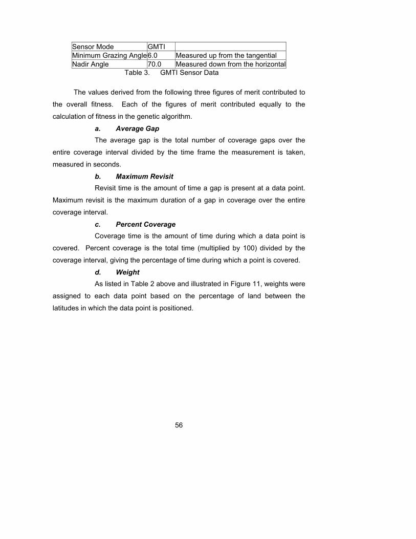
56

Sensor Mode GMTI Minimum Grazing Angle 6.0 Measured up from the tangential Nadir Angle 70.0 Measured down from the horizontal

Table 3. GMTI Sensor Data The values derived from the following three figures of merit contributed to

the overall fitness. Each of the figures of merit contributed equally to the

calculation of fitness in the genetic algorithm.

a. Average Gap The average gap is the total number of coverage gaps over the

entire coverage interval divided by the time frame the measurement is taken,

measured in seconds.

b. Maximum Revisit Revisit time is the amount of time a gap is present at a data point.

Maximum revisit is the maximum duration of a gap in coverage over the entire

coverage interval.

c. Percent Coverage Coverage time is the amount of time during which a data point is

covered. Percent coverage is the total time (multiplied by 100) divided by the

coverage interval, giving the percentage of time during which a point is covered.

d. Weight As listed in Table 2 above and illustrated in Figure 11, weights were

assigned to each data point based on the percentage of land between the

latitudes in which the data point is positioned.

57

Latitude Weight Derived from Land Area

0.026

0.1080.109

0.1200.116

0.112

0.086

0.0740.0750.0700.068

0.027

0.0070.002

0.00

0.02

0.04

0.06

0.08

0.10

0.12

0.14

75 N65 N55 N45 N35 N25 N15 N5 N5 S15 S25 S35 S45 S55 S

Latitude (deg)

Wei

ght

Figure 11. Weight by Latitude

e. Overall Fitness

Overall fitness was calculated using the three figures of merit

together with the weighted values determined for each data point. The equation

used for each data point is:

average gap maximum revisit percent coverageweight 186400 86400 100

⎧ ⎫⎡ ⎤⎛ ⎞ ⎛ ⎞ ⎛ ⎞∗ + + −⎨ ⎬⎜ ⎟ ⎜ ⎟ ⎜ ⎟⎢ ⎥⎝ ⎠ ⎝ ⎠ ⎝ ⎠⎣ ⎦⎩ ⎭ (5.1)

All data point sub totals were added together to generate the overall fitness

number we used to compare the genetic algorithm constellations against the

traditional Walker constellations.

C. RESULTS The orbital elements for all of the constellations designed and evaluated

are listed in Appendix B. The complete fitness calculations for all of the

constellations evaluated are included in Appendix C.

58

1. 9-ball Constellations The traditional 9-ball constellation designed had three orbital planes with

three satellites per plane; the complete orbital parameters are listed in Appendix

B. By applying Equation 5.1, the total fitness score for the 9-ball Walker

constellation was 0.793. The genetic algorithm designed constellation orbital

parameters are also listed in Appendix B. The total fitness score for the 9-ball

genetic algorithm design was 0.673. Fitness score calculations for the 9-ball

constellations are included in Appendix C. Figures 12-14 compare the average

revisit, maximum gap, and percent coverage of the 9-ball Walker and the 9-ball

GA design.

Comparison of 9-ball Constellation Average Revisit Time

0

1000

2000

3000

4000

5000

6000

7000

8000

9000

10000

55 S 45 S 35 S 25 S 15 S 5 S 5 N 15 N 25 N 35 N 45 N 55 N 65 N 75 N

Latitude (deg)

Ave

rage

Rev

isit

(s)

9-ball GA 9-ball Walker

Figure 12. Comparison of 9-ball Constellation Average Revisit Time

The 9-ball GA has a faster average revisit and lower maximum gap than

the 9-ball Walker between the latitudes of 15° and 35° both north and south and

at 75° north latitude.

59

Comparison of 9-ball Constellation Maximum Gap Time

0

2000

4000

6000

8000

10000

12000

14000

16000

55 S 45 S 35 S 25 S 15 S 5 S 5 N 15 N 25 N 35 N 45 N 55 N 65 N 75 N

Latitude (deg)

Max

imum

Gap

(s)


Figure 13. Comparison of 9-ball Constellation Maximum Gap Time

Comparing percent coverage, the 9-ball GA design outperforms the 9-ball

Walker at all latitudes.

60

Comparison of 9-ball Constellation Coverage

0

10

20

30

40

50

60

70

80

90

100

55 S 45 S 35 S 25 S 15 S 5 S 5 N 15 N 25 N 35 N 45 N 55 N 65 N 75 N

Latitude (deg)

Cov

erag

e (%

)9-ball GA 9-ball Walker

Figure 14. Comparison of 9-ball Constellation Percent Coverage

2. 12-ball Constellations The traditional 12-ball constellation designed had four orbital planes with



constellation was 0.650. The genetic algorithm designed 12-ball constellation

orbital parameters are also listed in Appendix B. The total fitness score for the

12-ball genetic algorithm design was 0.576. Fitness score calculations for the

12-ball constellations are included in Appendix C. Figures 15-17 compare the

average revisit, maximum gap, and percent coverage of the 12-ball Walker and

the 12-ball GA design.

61


0

500

1000

1500

2000

2500

3000

3500

4000

4500

5000

55 S 45 S 35 S 25 S 15 S 5 S 5 N 15 N 25 N 35 N 45 N 55 N 65 N 75 N

Latitude (deg)

Ave

rage

Rev

isit

(s)



The average revisit and maximum gap of the 12-ball GA design

outperformed the 12-ball Walker design between 15 ° north and south latitudes

and at the extreme northern latitude.

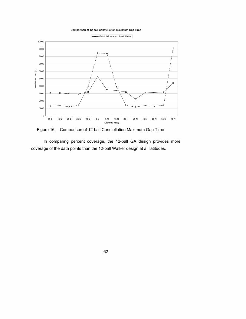
62


0

1000

2000

3000

4000

5000

6000

7000

8000

9000

10000

55 S 45 S 35 S 25 S 15 S 5 S 5 N 15 N 25 N 35 N 45 N 55 N 65 N 75 N

Latitude (deg)

Max

imum

Gap

(s)



In comparing percent coverage, the 12-ball GA design provides more

coverage of the data points than the 12-ball Walker design at all latitudes.

63


0

10

20

30

40

50

60

70

80

90

100

55 S 45 S 35 S 25 S 15 S 5 S 5 N 15 N 25 N 35 N 45 N 55 N 65 N 75 N

Latitude (deg)

Cov

erag

e (%



3. 18-ball Constellations The traditional 18-ball constellation designed had six orbital planes with



constellation was 0.456. The genetic algorithm designed 18-ball constellation

orbital parameters are also listed in Appendix B. The total fitness score for the

18-ball genetic algorithm design was 0.386. Fitness score calculations for the

18-ball constellations are included in Appendix C. Figures 18-20 compare the

average revisit, maximum gap, and percent coverage of the 18-ball Walker and

the 18-ball GA design.

64


0

200

400

600

800

1000

1200

1400

1600

1800

55 S 45 S 35 S 25 S 15 S 5 S 5 N 15 N 25 N 35 N 45 N 55 N 65 N 75 N

Latitude (deg)

Ave

rage

Rev

isit

(s)



The average revisit of the 12-ball GA design outperformed the 12-ball

Walker design only at 5° north, 65° north, and 75° north latitude. The

maximum gap time of the 18-ball GA design outperformed the 18-ball Walker

constellation at 75° north latitude only.

65


0

1000

2000

3000

4000

5000

6000

7000

55 S 45 S 35 S 25 S 15 S 5 S 5 N 15 N 25 N 35 N 45 N 55 N 65 N 75 N

Latitude (deg)

Max

imum

Gap

(s)



Although the 18-ball GA design did not perform as well as the 18-ball

Walker design in average revisit time or maximum gap time at most latitudes, it

did provide greater coverage at all latitudes.

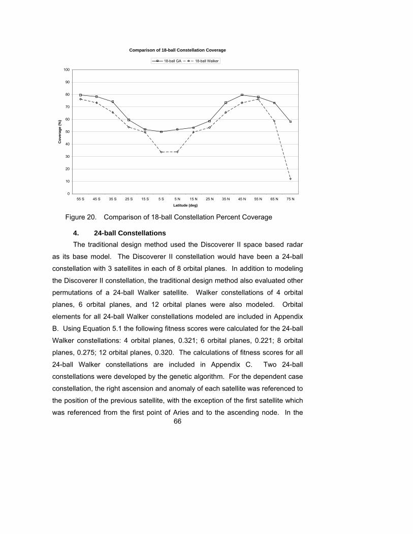
66


0

10

20

30

40

50

60

70

80

90

100

55 S 45 S 35 S 25 S 15 S 5 S 5 N 15 N 25 N 35 N 45 N 55 N 65 N 75 N

Latitude (deg)

Cov

erag

e (%



4. 24-ball Constellations The traditional design method used the Discoverer II space based radar

as its base model. The Discoverer II constellation would have been a 24-ball

constellation with 3 satellites in each of 8 orbital planes. In addition to modeling

the Discoverer II constellation, the traditional design method also evaluated other

permutations of a 24-ball Walker satellite. Walker constellations of 4 orbital

planes, 6 orbital planes, and 12 orbital planes were also modeled. Orbital

elements for all 24-ball Walker constellations modeled are included in Appendix

B. Using Equation 5.1 the following fitness scores were calculated for the 24-ball

Walker constellations: 4 orbital planes, 0.321; 6 orbital planes, 0.221; 8 orbital

planes, 0.275; 12 orbital planes, 0.320. The calculations of fitness scores for all

24-ball Walker constellations are included in Appendix C. Two 24-ball

constellations were developed by the genetic algorithm. For the dependent case

constellation, the right ascension and anomaly of each satellite was referenced to

the position of the previous satellite, with the exception of the first satellite which

was referenced from the first point of Aries and to the ascending node. In the

67

independent case, the right ascension and anomaly of all the satellites were

referenced from the first point of Aries and the ascending node. The orbital

elements for both of the GA designed 24-ball constellations are listed in

Appendix B. The 24-ball, dependent case GA designed constellation and the 24-

ball, independent case GA constellation had fitness scores of 0.276. Complete

fitness score calculations can be found in Appendix C. In Figures 21-23 below,

the performance of the 24-ball independent case GA design; 24-ball, 6 orbital

plane Walker; and the 24-ball, 8 orbital plane Walker are compared.


0

200

400

600

800

1000

1200

1400

55 S 45 S 35 S 25 S 15 S 5 S 5 N 15 N 25 N 35 N 45 N 55 N 65 N 75 N

Latitude (deg)

Ave

rage

Rev

isit

(s)

24-ball GA 24-ball Walker: 6 planes 24-ball Walker: 8 planes


The 24-ball GA designed constellation outperforms the two Walker

constellations only at 75° north latitude. The GA design outperforms the 8-plane

Walker at 5° north and south latitude as well.

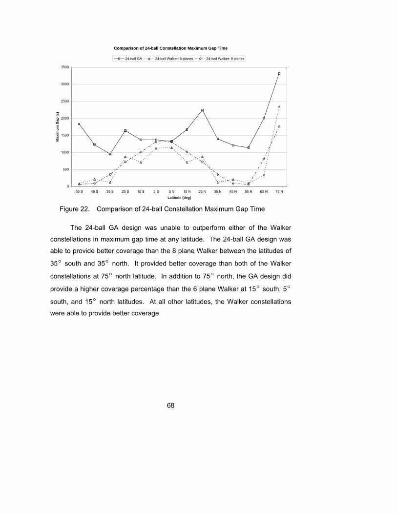
68


0

500

1000

1500

2000

2500

3000

3500

55 S 45 S 35 S 25 S 15 S 5 S 5 N 15 N 25 N 35 N 45 N 55 N 65 N 75 N

Latitude (deg)

Max

imum

Gap

(s)

24-ball GA 24-ball Walker: 6 planes 24-ball Walker: 8 planes


The 24-ball GA design was unable to outperform either of the Walker

constellations in maximum gap time at any latitude. The 24-ball GA design was

able to provide better coverage than the 8 plane Walker between the latitudes of

35° south and 35° north. It provided better coverage than both of the Walker

constellations at 75° north latitude. In addition to 75° north, the GA design did

provide a higher coverage percentage than the 6 plane Walker at 15° south, 5°

south, and 15° north latitudes. At all other latitudes, the Walker constellations

were able to provide better coverage.

69


0

10

20

30

40

50

60

70

80

90

100

55 S 45 S 35 S 25 S 15 S 5 S 5 N 15 N 25 N 35 N 45 N 55 N 65 N 75 N

Latitude (deg)

Cov

erag

e (%

)24-ball GA 24-ball Walker: 6 planes 24-ball Walker: 8 planes


D. SUMMARY

As Table 4 indicates, the constellations of 9, 12 and 18 satellites created

using a genetic algorithm did perform better than the constellations of 9, 12 and

18 satellites using traditional constellation design methods. With 9, 12, or 18

satellites per constellation, the best performance in terms of average revisit and

maximum gap was a function of the latitude, with the genetic algorithm

performing better near the equator and at the northernmost latitude and the

Walker constellations performing better at the mid-latitudes. However, in 9-ball,

12-ball, and 18-ball constellations, the genetic algorithm outperformed the Walker

constellation in percent coverage at every latitude.

However, the 24 satellite genetic algorithm constellations were unable to

out perform all of the traditional 24 satellite Walker constellations. The 24-ball

genetic algorithm constellations were able to achieve better fitness scores than

the 24-ball Walker constellations of 4 planes and 12 planes. The GA

constellations performed nearly as well as the 8 plane Walker constellation which

70

modeled the proposed Discoverer II space based radar system. Clearly the 24-

ball GA constellations were dominated by the performance of the 24-ball, 6 plane

Walker constellation.

Fitness

GA Design 0.673

3-plane Walker 0.793

GA Design 0.576


GA Design 0.386


GA Design, Dependent Case 0.276

GA Design, Independent Case 0.276



8-plane Walker, Discoverer II 0.275


24-b

all

Constellation

9-ba

ll12

-bal

l18

-bal

l

Table 4. Summary of Fitness Scores for Designed Constellations

There are two possible explanations why the genetic algorithm was not

able to design a constellation that could outperform the best 24-ball Walker

constellation. The first possibility is that the termination criteria selected for the

genetic algorithm, 100 generations with no improvement in the fitness score of

the fittest individual, did not permit the genetic algorithm to thoroughly search the

complex search space of a 24 satellite constellation. The second explanation is

that as the number of satellites increases and the constellation becomes less

sparse, a Walker constellation provides nearly optimal performance. In either

case, the answer was beyond the scope of this thesis. Further study modifying

71

the termination criteria will determine if the first hypothesis is true. If the first

hypothesis is false, further study to investigate the number of satellites where a

genetic algorithm design can no longer outperform a Walker constellation is

indicated.

72


73

VI. THE BENEFITS OF SUPERIORITY

A. THE THREAT The uncertainty among security officials is not if al-Qaeda will attack

again, but when. Equally important questions are where and how. One theory

on how the next attack will occur is via the sea. Specifically, many security

officials believe al-Qaeda will acquire a merchant ship and use it as a floating

bomb or blow up a merchant ship similar to the attack on the USS Cole.

An article entitled Merchant Shipping 'At Risk of Attack', by Michael Evans,

was recently published in the London Times. In his article, Mr. Evans writes of

Admiral Sir Alan West, the head of the Royal Navy, stating al-Qaeda is plotting to

blow up merchant ships. According to Mr. Evans, Admiral West stated, "What we

have noticed is that al-Qaeda and other organizations have an awareness about

maritime trade. They've realized how important it is for world trade in general

(and) they understand that significance." Admiral West revealed, "We have seen

plans from intelligence of (proposed) attacks on merchant shipping. We are

aware that they have plans and they have looked at this."

Attacks on the French supertanker, Limburg, and the USS COLE prove al-

Qaeda is willing and able to attack ships. However, most susceptible militaries

have increased security on and around their vessels leaving merchant vessels as

the most likely target.

As Admiral West points out, it is very difficult to attack a ship on the open

sea. Therefore, the most likely target will be in ports and maritime choke points.

According to Michael Evans, "A suspected al-Qaeda cell was arrested in

Morocco two years ago after a plot was exposed to attack shipping in the Strait of

Gibraltar." As a result, following the thwarted attack, western merchant ships

were assigned escorts through the Strait.

Escorting merchant ships in and out of port and through straits is certainly

effective, but not efficient. The escort ships are being pulled from their primary

74

mission and the number of merchant ship targets outnumbers the number of

available escorts. An alternate solution should be explored. [26]

B. A POSSIBLE SOLUTION 1. The Theory A number of assumptions are implicit regarding the concept of operations

of a space based radar system in the equations derived below. First, the satellite

will be given the initial position of a track of interest. Second, the constellation

will have a common track correlation database and tasking system so that

information about a track generated by one satellite is available to all satellites.

Third, the satellite system will be able to identify a specific track with SAR

imagery. Finally, the SAR will be able to image all candidate tracks designated by

the GMTI sensor and no time delay exists in switching between SAR and GMTI

modes.

With these assumptions in mind, the number of tracks a space based

radar system can maintain can be derived from either the maximum gap time or

the average revisit time of the constellation. If the space based radar system

operates autonomously, receiving no data from other sources to help maintain a

track, the maximum gap is used in calculating the number of tracks maintained.

If the space based radar has the ability to receive cues or supplemental data

from other sources to assist in maintaining a track, average revisit time should be

used in calculating the number of tracks maintained.

The number of tracks maintained is equal to the time an area is in view

divided by the time it takes to locate a specific track.

Number of tracks maintained Time an area is in view Time to locate a track

NTvTl

TvNTl

≡≡≡

=

The time required to locate a specific track is equal to the time required to

search for a track added to the time to identify a track.

75

Time required to search for a track Time required to identify a track

TsTiTl Ts Ti

≡≡= +

The time required to search for a specific track is equal to the search area

divided by the search rate.

Search area Search rate

SaSr

SaTsSr

≡≡

=

The time required to identify a specific track is equal to the number of

candidate tracks multiplied by the time to image one track. On average, the

system will have to image half of the candidate tracks to locate a specific track.

Number of candidate tracks Time to image a track

1 * *2

NcTsar

Ti Nc Tsar

≡≡

=

The number of candidate targets equals the area of uncertainty multiplied

by the target density.

Area of uncertainty Target density

*

AuTdNc Au Td

≡≡=

The search area equals the area of uncertainty which is the area of the

circle with radius equal to the revisit time multiplied by the target velocity.

( )2

Revisit time Target velocity

* *

TrVt

Sa Au Tr Vtπ

≡≡

= =

Substituting and simplifying.

76

( )

( ) ( )

( )

( )

2

22

2

2

1 * *2

* * 1 * * *2

* * 1 * * * * *2

1 ** *2

2 * ** *2*

TvNTl

TvNTs Ti

TvNSa Nc TsarSr

TvNTr Vt

Au Td TsarSr

TvNTr Vt

Tr Vt Td TsarSr

TvNTd TsarTr Vt

SrTvN

Sr Td TsarTr VtSr

π

ππ

π

π

=

=+

=⎛ ⎞ ⎛ ⎞+⎜ ⎟ ⎜ ⎟⎝ ⎠ ⎝ ⎠

=⎛ ⎞ ⎛ ⎞+⎜ ⎟ ⎜ ⎟⎜ ⎟ ⎝ ⎠⎝ ⎠

=⎛ ⎞ ⎛ ⎞+⎜ ⎟ ⎜ ⎟⎜ ⎟ ⎝ ⎠⎝ ⎠

=⎛ ⎞∗ +⎜ ⎟⎝ ⎠

=+⎛ ⎞∗⎜

⎝

( ) ( )22* *

* * 2 * *Tv SrN

Tr Vt Sr Td Tsarπ

⎟⎠

=∗ +

The average time in view for a point is approximately 0.63 times the

maximum time in view for a point, based on a circular footprint. In addition, the

search area (area of uncertainty) may or may not be completely within by the

footprint. The space based radar system cannot reliably maintain track on a

target if the area of uncertainty is not completely covered by sensor footprint.

The calculation of tracks maintained discounts a track if any portion of the area of

uncertainty falls outside the sensor footprint. This is accounted for by taking the

inverse of the ratio of the radius of the search area to the radius of the footprint.

( ) ( )

( )

2

2 2 2

Radius of the access footprint

* 2 2* *1- * ** * 2 * *

* 4* *1- ** * * 2 * *

Rf

Tr Vt Tv SrNRf Tr Vt Sr Td Tsar

Tr Vt Tv SrNRf Tr Vt Sr Td Tsar

π π

π

≡

⎛ ⎞= ⎜ ⎟ ∗ +⎝ ⎠

⎛ ⎞= ⎜ ⎟ +⎝ ⎠

77

2. The Math The equations derived above can next be applied with the figure of merit

values calculated for the constellations designed. The example below is the

calculation of the number of tracks maintained by the Discoverer II constellation

at 35 N°based on average revisit time, the latitude of San Francisco, CA and

Washington, D.C.

To calculate the radius of the sensor footprint, it is necessary to know the

elevation or grazing angle and the altitude of the satellite. The figure below

illustrates the geometry of the earth, satellite, and target which is used in deriving

the footprint radius. The radius of the footprint is the distance from the

subsatellite point to the target which equals the earth central angle times the

radius of the earth.

Figure 24. Geometry between the Earth, Satellite, and Target [After 5] Formatted: Bullets and Numbering

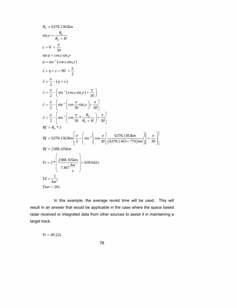
78

( )

( )

( )

1

1

1

1

6378.1363

sin

630

sin cos sinsin cos sin

902

2

sin cos sin2 30

sin cos sin2 30 30

sin cos *2 30 30

*

6378.1

E

E

E

E

E

E

R kmR

R H

RR H

Rf R

Rf

ρ

πε

η ε ρ

η ε ρπλ η ε

πλ η ε

π πλ ε ρ

π π πλ ρ

π π πλ

λ

−

−

−

−

=

=+

= =

=

=

+ + = =

= − +

⎛ ⎞= − +⎜ ⎟⎝ ⎠⎡ ⎤⎛ ⎞= − +⎜ ⎟⎢ ⎥⎝ ⎠⎣ ⎦⎡ ⎤⎛ ⎞

= − +⎢ ⎥⎜ ⎟+⎝ ⎠⎣ ⎦=

=

o

o

( )1

2

6378.1363363 sin cos2 30 6378.1363 770 30

2388.105

2388.1052 * 639.6427.467

1

20

kmkmkm

Rf km

kmTv skms

Tdkm

Tsar s

π π π−⎡ ⎤⎛ ⎞⎧ ⎫⎡ ⎤⎪ ⎪⎢ ⎥− +⎜ ⎟⎨ ⎬⎢ ⎥⎜ ⎟+⎢ ⎥⎪ ⎪⎣ ⎦⎩ ⎭⎝ ⎠⎣ ⎦

=

⎛ ⎞⎜ ⎟

= =⎜ ⎟⎜ ⎟⎝ ⎠

=

=

In this example, the average revisit time will be used. This will

result in an answer that would be applicable in the case where the space based

radar received or integrated data from other sources to assist it in maintaining a

target track.

49.22Tr s=

79

The GMTI sensor search rate is dependent on altitude and target

velocity. It was necessary to develop an equation for search rate that would

enable the comparison of constellations at different altitudes. Toyon Research

provided the sensor data from which the search rate equations were derived.

The data were provided for a GMTI sensor at altitudes of 1000 km and 10000km

and for target velocities of 4 kph, 8kph, and 16kph. The equations derived were

linear extrapolations of the data provided. The data and the equations are

summarized in the table below; search rate is in km 2 /s.

Altitude 4 kph 8 kph 16 kph1000 km 105 258 107410000 km 527 1044 1233

Derived Equation y = 0.0469x + 58.111 y = 0.0873x + 170.67 y = 0.0177x + 1056.3

Target Velocity

Table 5. Search Rate Data and Equations

In this example, the number of tracks maintained will be calculated

for a target velocity of 4 kph.

( ) ( )2

4 0.00111

0.0469 58.111 0.0469 770 58.111 94.224

km kmVth s

kmSr altitudes

= =

= + = + =

Now that all of the known variables have been identified and

defined, the number of 4 kph tracks maintained by the Discoverer II constellation

at 35 N can be calculated.

80

( )2 2

22

25

2

5

49.22 * 0.00111 0.0094010.00940 * 0.00940

1 * 0.00940 * 20 0.094020.00940 9.972 *1094.224

0.0940 9.972 *10 0.0941

49.22 * 0.00111639.642 10.0941 2388.105

Sa Au km

Nc kmkm

Ti s s

kmTs skm

sTl s s s

kmss sNs km

π

−

−

= = =

= =

= =

= =

= + =

⎛ ⎞= −⎜ ⎟⎝ ⎠

6799.898 6800

⎛ ⎞⎜ ⎟

= ≈⎜ ⎟⎜ ⎟⎝ ⎠

3. The Solution By repeating the calculation above for the fittest constellations designed,

the number of tracks reliably maintained by each constellation can be calculated.

The number of tracks maintained varies by latitude, the target’s velocity, and

track density. Figures 13, 14, 15, and 16 illustrate the number of tracks

maintained by latitude and target velocity for the 24-ball Walker constellation, the

18-ball GA constellation, the 12-ball GA constellation, and the 9-ball GA

constellation, respectively. These results were calculated using average revisit

time and a track density of 1/km 2 . Calculating the number of tracks maintained

using average revisit time models the performance of a space based radar

system that could integrate data or receive track information from other sources.

In all of the graphs, a significant decrease in performance is evident at the lower

latitudes.

81

6 plane, 24 ball Walker Constellation Performance Derived from Average Revisit Time

1

10

100

1000

10000

100000

1000000

10000000

55 S 45 S 35 S 25 S 15 S 5 S 5 N 15 N 25 N 35 N 45 N 55 N 65 N 75 N

Latitude (deg)

Trac

ks

(log

scal

e)16 kph 8 kph 4 kph

Figure 25. 24-ball Walker Performance

18 ball GA Constellation Performance Derived from Average Revisit Time

1

10

100

1000

10000

55 S 45 S 35 S 25 S 15 S 5 S 5 N 15 N 25 N 35 N 45 N 55 N 65 N 75 N

Latitude (deg)

Trac

ks(lo

g sc

ale)

16 kph 8 kph 4 kph

Figure 26. 18-ball GA Performance

82


0

10

20

30

40

50

60

55 S 45 S 35 S 25 S 15 S 5 S 5 N 15 N 25 N 35 N 45 N 55 N 65 N 75 N

Latitude (deg)

Trac

ks16 kph 8 kph 4 kph



0

5

10

15

20

25

30

35

55 S 45 S 35 S 25 S 15 S 5 S 5 N 15 N 25 N 35 N 45 N 55 N 65 N 75 N

Latitude (deg)

Trac

ks

16 kph 8 kph 4 kph


83

In the calculation of tracks maintained, only the average revisit time figure

of merit was used. This may raise the question why not modify the fitness

function so that the genetic algorithm would either only seek to minimize the

average revisit time or at least give the average revisit time more weight in the

calculation. That would be an option if the concept of operations of the space

based radar system specified that it would never operate autonomously and that

it only would be used for GMTI. However, the space based radar system will

have other functions that will not depend as heavily on average revisit time.

C. CONCLUSION If fielded, Discoverer II Space Based Radar Constellation would have

been able to track 6800 targets traveling at 4kph at 35 °N. Space based radar

constellations comprised of less than 24 satellites suffer a drop in performance.

However, if an SBR constellation is constrained to less than 24 satellites, genetic

algorithms offer a fitness improvement over traditional constellation design

methods. The critical step in implementing a genetic algorithm to design a

constellation is defining the fitness function in a manner that will translate into

performance gains.

D. FURTHER STUDY 1. Caveat These satellite constellation comparisons are based on revisit and

coverage performance only. Other considerations such as satellite dimensions,

sensor complexity, design timeline, acquisition resources or launch vehicles were

not included. Additionally, constellations were designed with the same sensor

capability in varying orbital patterns.

The consequence of not considering the parameters listed above is that

predictions cannot be made concerning the feasibility of the constellations

designed. For instance, a constellation designed by the genetic algorithm may

have performed better than traditional constellations. However, the cost of

launching satellites in many different orbital planes and into retrograde orbits may

be prohibitive.

84

2. Next Steps Follow on research should be conducted using the genetic algorithm from

this thesis as a constellation design tool. Additional runs of the genetic algorithm

should be conducted using a coverage definition consisting of a different set of

data points to validate the results. Rather than choosing either to have a

satellite’s position referenced to the previous satellite, the dependent case, or

referenced to a fixed point, the independent case, a combination of the two

methods could be implemented. This combination may result in the construction

of a parallel genetic algorithm that would build on the current genetic algorithm.

This could be accomplished by having the current genetic algorithm generate

satellites referenced to each other, the dependent case. Following the evaluation

of fitness, the fittest members of the population would go through an additional

step where the each satellite would be permitted to mutate independently and

this mutation evaluated. Additional work should be done in deriving constellation

performance (tracks maintained) from the figure of merit values. This may lead

to developing a better fitness function in which the figures of merit are not

weighed evenly. It may be desirable to have the number of tracks maintained by

a space based radar system remain nearly constant across all latitudes. Further

research should be conducted in the weights derived for the latitudes and the

derivation of the fitness function to reward the genetic algorithm for designing

constellations with similar revisit and gap statistics across all latitudes. The

genetic algorithm has demonstrated the ability to design sparse constellations

better than traditional Walker designs. Further study could be conducted to

determine if the genetic algorithm can design constellations achieving the same

level of performance as a Walker constellation with fewer satellites.

85

LIST OF REFERENCES

1. Vallado, D. A., Fundamentals of Astrodynamics and Applications, Second

Edition, Microcosm Press, El Segundo, California and Kluwer Academic

Publishers, Dordrecht, The Netherlands, 2001

2. Sellers, J. J., UNDERSTANDING SPACE An Introduction to Astronautics,

Second Edition, McGraw-Hill Companies, the United States of America,

2000

3. http://www.avmdynamics.com/images/software_07.jpg, referenced July

2004

4. http://www.avmdynamics.com/images/software_06.jpg, referenced July

2004

5. Wertz, J. R., Mission Geometry; Orbit and Constellation Design and

Management, Microcosm Press, El Segundo, California and Kluwer

Academic Publishers, Dordrecht, The Netherlands, 2001

6. Coley, D. A., An Introduction to Genetic Algorithms for Scientists and

Engineers, pp. 1-2, World Scientific Publishing Co. Pte. Ltd., Singapore,

1999

7. Karr, C. L. and Freeman, L. M., Industrial Applications of Genetic

Algorithms, CRC Press LLC, Boca Raton, Florida, 1999

8. Goldberg, D. E., Genetic Algorithms in Search, Optimization, and Machine

Learning, Addison-Wesley, Reading, Massachusetts, 1989

9. Michalewicz, Z., Genetic Algorithm + Data Structure = Evolution

Programs, 3rd edition, Springer-Verlag, New York, 1996

10. Gen, M. and Cheng, R., Genetic Algorithms and Engineering Optimization,

John Wiley & Sons, Inc., New York, New York, 2000

11. Mitchell, M., An Introduction to Genetic Algorithms, Massachusetts

Institute of Technology, Cambridge, Massachusetts, 1996

12. Olsen, R. C., Remote Sensing from Air and Space, PH3052 Class Notes,

Naval Postgraduate School, Monterey, California, 2003

86

13. http://www.public.iastate.edu/~hansen88/Radar/pics/RadarPulse.gif,

referenced July 2004

14. http://www.f-111.net/CarloKopp/gps.htm, referenced July 2004

15. Dunn, R. J. III, Bingham, P. T., Fowler, C. A., Ground Moving Target

Indicator Radar and the Transformation of U.S. Warfighting, Northrop

Grumman Analysis Center Papers, Washington D.C., February 2004

16. Tirpak, J. A., The Space Based Radar Plan, Vol.85, No. 08, Air Force,

Journal of the Air Force Association, Magazine Online, August 2002,

http://www.afa.org/magazine/aug2002/0802radar.asp, referenced July

2004

17. http://www.congress.gov/cgi-

bin/cpquery/?&&dbname=cp108&&&r_n=hr553.108&&sel=TOC_375491&,

House Rpt.108-553 – DEPARTMENT OF DEFENSE APPROPRIATIONS

BILL, 2005, referenced July 2004;

18. http://www.losangeles.af.mil/SMC/PA/Fact_Sheets/discoverer_2.pdf,

Discoverer II Joint Program Fact Sheet, Air Force, referenced July 2004;

19. http://www.congress.gov/cgi-

bin/cpquery/?&dbname=cp106&&r_n=hr644.106&sel=TOC_362215&,

House Rpt.106-644 - DEPARTMENT OF DEFENSE APPROPRIATIONS

BILL, 2001, referenced July 2004;

20. http://www.fas.org/spp/military/program/imint/starlight.htm, Kunkel, J.,

Discoverer II a DARPA SAR TACSAT, DARPA, November, 1998,

referenced July 2004

21. Lang, T. J., ”A Parametric Examination of Satellite Constellations To

Minimize Revisit Time For Low Earth Orbits Using a Genetic Algorithm “,

AAS 01-345, AAS/AIAA Astrodynamics Specialist Conference, Quebec

City, Quebec, Canada, 30 July – 2 Aug, 2001.

22. Crossley, W. A., and Williams, E. A., “Simulated Annealing and Genetic

Algorithm Approaches for Discontinuous Coverage Satellite Constellation

Design”, Engineering Optimization, Vol. 32, 1999-2000.

87

23. Williams, E. A., Crossley, W. A., and Lang, T. J., “Average and Maximum

Revisit Time Trade Studies for Satellite Constellations using a

Multiobjective Genetic Algorithm”, AAS 00-139, AAS/AIAA Space Flight

Mechanics Meeting, Clearwater, Florida, January 23-26, 2000.

24. http://www.stk.com/resources/download/download.cfm, referenced July

2004

25. http://www.oceansatlas.org/unatlas/about/physicalandchemicalproperties/

background/seemore1.htm, referenced July 2004

26. M. E. Evans, Merchant Shipping 'At Risk of Attack', London Times, 6

August, 2004, http://www.portsecuritystrategies.com/art8.htm, referenced

September 2004

88


89

APPENDIX A GENETIC ALGORITHM CODE

'COMPGA 'Constellation Optimization via Multi-Ploid Genetic

Algorithm 'Version 3.0 'Programmed by Douglas J. Pegher 'July 2004 Option Explicit 'dimension module constants and variables 'Integer value of last generation Const mLastGeneration As Integer = 20 'Population size; must be divisible by 3 Const mTotalConstellations As Integer = 9 'Number of satellites in constellation Const mSatelliteNumber As Integer = 24 'Number of orbital element variables ~ no

ecentricity, no arg. of perigee ~ alt. and inc. same for all sats

Const mOrbitalElement As Integer = 4 'Probability of crossover Const mCrossoverProbability As Single = 0.6 'Probability of mutation Const mMutationProbability As Single = 0.0625 'define semimajor axis range Const MinSemiMajorAxis As Single = 500 'min value Const MaxSemiMajorAxis As Single = 1000 'max value 'define inclination range Const MinInclination As Single = 0 'min value Const MaxInclination As Single = 180 'max value 'define rightascension range Const MinRightAscension As Single = 0 'min value Const MaxRightAscension As Single = 360 'max value Dim mPreviousRightAscension As Single 'define anomaly range Const MinAnomaly As Single = 0 'min value Const MaxAnomaly As Single = 360 'max value Dim mPreviousAnomaly As Single 'current generation counter Dim mCurrentGeneration As Integer 'data array Dim mGAArray(3, (mOrbitalElement - 1),

(mSatelliteNumber - 1), (mTotalConstellations - 1), (mLastGeneration - 1)) As Byte

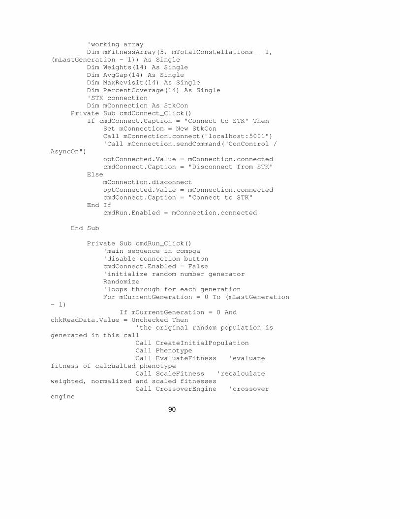
90

'working array Dim mFitnessArray(5, mTotalConstellations - 1,

(mLastGeneration - 1)) As Single Dim Weights(14) As Single Dim AvgGap(14) As Single Dim MaxRevisit(14) As Single Dim PercentCoverage(14) As Single 'STK connection Dim mConnection As StkCon Private Sub cmdConnect_Click() If cmdConnect.Caption = "Connect to STK" Then Set mConnection = New StkCon Call mConnection.connect("localhost:5001") 'Call mConnection.sendCommand("ConControl /

AsyncOn") optConnected.Value = mConnection.connected cmdConnect.Caption = "Disconnect from STK" Else mConnection.disconnect optConnected.Value = mConnection.connected cmdConnect.Caption = "Connect to STK" End If cmdRun.Enabled = mConnection.connected End Sub Private Sub cmdRun_Click() 'main sequence in compga 'disable connection button cmdConnect.Enabled = False 'initialize random number generator Randomize 'loops through for each generation For mCurrentGeneration = 0 To (mLastGeneration

- 1) If mCurrentGeneration = 0 And

chkReadData.Value = Unchecked Then 'the original random population is

generated in this call Call CreateInitialPopulation Call Phenotype Call EvaluateFitness 'evaluate

fitness of calcualted phenotype Call ScaleFitness 'recalculate

weighted, normalized and scaled fitnesses Call CrossoverEngine 'crossover

engine

91

ElseIf mCurrentGeneration = 0 And chkReadData.Value = Checked Then

Call ReadData Call Phenotype Call EvaluateFitness 'evaluate



engine Else Call MatingCoupler 'mating engine Call MutationEngine 'mutation engine Call Phenotype Call CopyFitnessArray ' copies

previous fitness scores into current generation Call EvaluateFitness 'evaluate



engine End If Next mCurrentGeneration cmdDisplay.Enabled = mConnection.connected cmdConnect.Enabled = True 'when GOMPGA is finished running write all

data to file. Call WriteData Call WriteFitness End Sub Private Sub CreateInitialPopulation() 'called from Private Sub btnRun_Click 'create initial population 'dimension subprocedure variables Dim Constellation As Integer Dim Satellite As Integer Dim OrbitalElement As Integer Dim Genotype As Integer 'loop through GAArray assigning random numbers

to the data cells for the first generation 'random numbers range from 32767 to -32768 'random numbers of 0.9999847412109375 and

greater yield 32767

92

'random numbers of less than 0.0000152587890625 yield -32768

'the short data type represents the values of -32768 to 32767 as 16 bit binary

'as binary strings the values range from 0 up to 32767 and then -32768 to -1

'-1 is represented as 16 ones For Constellation = 0 To (mTotalConstellations

- 1) For Satellite = 0 To (mSatelliteNumber -

1) For OrbitalElement = 0 To

(mOrbitalElement - 1) For Genotype = 0 To 2 mGAArray(Genotype,

OrbitalElement, Satellite, Constellation, mCurrentGeneration) = CByte(255 * Rnd())

Next Genotype Next OrbitalElement Next Satellite Next Constellation End Sub Private Sub Phenotype() 'called from Private Sub

CreateInitialPopulation 'called from Private Sub Mutation 'calculate phenotypes for most recently

created generation 'dimension subprocedure variables Dim Constellation As Integer Dim Satellite As Integer Dim OrbitalElement As Integer 'loop through current generation and calcualte

phenotypes 'phenotype is the result of the bitwise

comparison of the three genotype values 'the bit is decided by a simple majority of

the bits in the genotype For Constellation = 0 To (mTotalConstellations



(mOrbitalElement - 1)

93

mGAArray(3, OrbitalElement, Satellite, Constellation, mCurrentGeneration) = ((mGAArray(1, OrbitalElement, Satellite, Constellation, mCurrentGeneration) And mGAArray(2, OrbitalElement, Satellite, Constellation, mCurrentGeneration)) Or (mGAArray(2, OrbitalElement, Satellite, Constellation, mCurrentGeneration) And mGAArray(3, OrbitalElement, Satellite, Constellation, mCurrentGeneration)) Or (mGAArray(3, OrbitalElement, Satellite, Constellation, mCurrentGeneration) And mGAArray(1, OrbitalElement, Satellite, Constellation, mCurrentGeneration)))

Next OrbitalElement Next Satellite Next Constellation End Sub Private Sub EvaluateFitness() 'called from Private Sub Phenotype 'evaluate fitness of current generation 'dimension variables Dim Constellation As Integer Dim Satellite As Integer Dim Fitness As Single Dim NewSatelliteString As String Dim NewSensorString As String Dim OrbitalElementString As String Dim SetStateString As String Dim SatellitePath As String Dim SensorPath As String Dim CoveragePath As String Dim AvgGapReportPath As String Dim MaxRevisitReportPath As String Dim PercentCoverageReportPath As String Dim Counter As Integer Dim AvgGapFitness As Single Dim MaxRevisitFitness As Single Dim PercentcoverageFitness As Single Weights(0) = 0 'unused Weights(14) = 0.071379704 '75deg N Weights(13) = 0.180843786 '65deg N Weights(12) = 0.134321551 '55deg N Weights(11) = 0.11972634 '45deg N Weights(10) = 0.099885975 '35deg N Weights(9) = 0.087571266 '25deg N Weights(8) = 0.062941847 '15deg N

94

Weights(7) = 0.052451539 '5deg N Weights(6) = 0.05359179 '5deg S Weights(5) = 0.051083238 '15deg S Weights(4) = 0.05313569 '25deg S Weights(3) = 0.023717218 '35deg S Weights(2) = 0.007069555 '45deg S Weights(1) = 0.002280502 '55deg S CoveragePath =

"*/CoverageDefinition/55s_75n_10deg" AvgGapReportPath = CoveragePath &

"/FigureOfMerit/Avg_Gap ""Avg Gap""" MaxRevisitReportPath = CoveragePath &

"/FigureOfMerit/Max_Revisit ""Max Revisit""" PercentCoverageReportPath = CoveragePath &

"/FigureOfMerit/Percent_Coverage ""Percent Coverage""" 'convert the phenotype short into a positive

integer ~ conversion in functions 'send positive integer to be scaled ~ scale

range defined in functions 'determine fitness 'a lower fitness is better 'fitness is evaluated by generation, but the

fitness array is updated for each individual constellation For Constellation = 0 To (mTotalConstellations

- 1) 'create new constellation For Satellite = 0 To (mSatelliteNumber -

1) 'create new satellite NewSatelliteString = "New / */Satellite "

& Satellite mConnection.sendCommand

(NewSatelliteString) 'input satellite ephemeris OrbitalElementString =

SemiMajorAxis(mGAArray(3, 0, 0, Constellation, mCurrentGeneration)) & " 0.0 " & Inclination(mGAArray(3, 1, 0, Constellation, mCurrentGeneration)) & " 0.0 " & RightAscension(mGAArray(3, 2, Satellite, Constellation, mCurrentGeneration), Satellite) & " " & Anomaly(mGAArray(3, 3, Satellite, Constellation, mCurrentGeneration), Satellite)

SatellitePath = "*/Satellite/" & Satellite 'SetState Scenario/stkDemo/Satellite/ERS1

Classical J2Perturbation "1 Nov 2000 00:00:00.00" "1 Nov

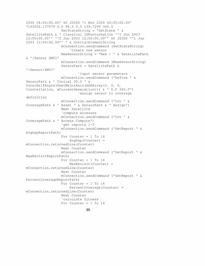
95

2000 04:00:00.00" 60 J2000 "1 Nov 2000 00:00:00.00" 7163000.137079 0.0 98.5 0.0 139.7299 360.0

SetStateString = "SetState " & SatellitePath & " Classical J2Perturbation ""1 Jun 2003 12:00:00.00"" ""2 Jun 2003 12:00:00.00"" 60 J2000 ""1 Jun 2003 12:00:00.00"" " & OrbitalElementString

mConnection.sendCommand (SetStateString) 'create new sensor NewSensorString = "New / " & SatellitePath

& "/Sensor SMTI" mConnection.sendCommand (NewSensorString) SensorPath = SatellitePath &

"/Sensor/SMTI" 'input sensor parameters mConnection.sendCommand ("Define " &

SensorPath & " Conical 20.0 " & OuterHalfAngle(SemiMajorAxis(mGAArray(3, 0, 0, Constellation, mCurrentGeneration))) & " 0.0 360.0")

'assign sensor to coverage definition

mConnection.sendCommand ("Cov " & CoveragePath & " Asset " & SensorPath & " Assign")

Next Satellite 'compute accesses mConnection.sendCommand ("Cov " &

CoveragePath & " Access Compute") 'get reports 1-3 mConnection.sendCommand ("GetReport " &

AvgGapReportPath) For Counter = 1 To 14 AvgGap(Counter) =

mConnection.returnedLine(Counter) Next Counter mConnection.sendCommand ("GetReport " &

MaxRevisitReportPath) For Counter = 1 To 14 MaxRevisit(Counter) =

mConnection.returnedLine(Counter) Next Counter mConnection.sendCommand ("GetReport " &

PercentCoverageReportPath) For Counter = 1 To 14 PercentCoverage(Counter) =

mConnection.returnedLine(Counter) Next Counter 'calculate fitness For Counter = 1 To 14

96

Fitness = Fitness + (Weights(Counter) * ((AvgGap(Counter) / 86400) + (MaxRevisit(Counter) / 86400) + (1 - (PercentCoverage(Counter) / 100))))

Next Counter 'update fitness array Call FitnessArray(Constellation, Fitness) Fitness = 0 'clear accesses mConnection.sendCommand ("Cov " &

CoveragePath & " Access Clear") 'unload constellation mConnection.sendCommand ("UnloadMulti /

*/Satellite/*") Next Constellation End Sub Private Sub FitnessArray(ByVal Constellation As

Integer, ByVal Fitness As Single) 'called from Private Sub EvaluateFitness 'compare a constellation to current fitest

constellations and replace the less fit 'dimension subprocedure variables Dim FitnessColumn As Integer 'loop through fitness array and compare

candidate constellation fitness to previous constellation fitness

'fitness in the test function is arranged from low to high, low fitnesses are better

If mCurrentGeneration = 0 Then For FitnessColumn = 0 To Constellation If FitnessColumn < Constellation And

Fitness < mFitnessArray(2, FitnessColumn, mCurrentGeneration) Then

Call ChangeOrder(FitnessColumn) mFitnessArray(0, FitnessColumn,

mCurrentGeneration) = Constellation mFitnessArray(1, FitnessColumn,

mCurrentGeneration) = mCurrentGeneration mFitnessArray(2, FitnessColumn,

mCurrentGeneration) = Fitness Exit For ElseIf FitnessColumn = Constellation

Then mFitnessArray(0, FitnessColumn,

mCurrentGeneration) = Constellation

97

mFitnessArray(1, FitnessColumn, mCurrentGeneration) = mCurrentGeneration

mFitnessArray(2, FitnessColumn, mCurrentGeneration) = Fitness

End If Next FitnessColumn ElseIf mCurrentGeneration <> 0 Then For FitnessColumn = 0 To

(mTotalConstellations - 1) If Fitness < mFitnessArray(2,

FitnessColumn, mCurrentGeneration) Then Call ChangeOrder(FitnessColumn) mFitnessArray(0, FitnessColumn,

mCurrentGeneration) = Constellation mFitnessArray(1, FitnessColumn,

mCurrentGeneration) = mCurrentGeneration mFitnessArray(2, FitnessColumn,

mCurrentGeneration) = Fitness Exit For End If Next FitnessColumn End If End Sub Private Sub ChangeOrder(ByVal FitnessColumn As

Integer) 'called from Private Sub FitnessArray 'update fitness array 'dimension subprocedure variables Dim Column As Integer 'loop through fitness array in reverse order

and shift constellation order 'this copies the next best fitness into the

current cell For Column = (mTotalConstellations - 1) To

(FitnessColumn + 1) Step -1 mFitnessArray(0, Column,

mCurrentGeneration) = mFitnessArray(0, Column - 1, mCurrentGeneration)

mFitnessArray(1, Column, mCurrentGeneration) = mFitnessArray(1, Column - 1, mCurrentGeneration)

mFitnessArray(2, Column, mCurrentGeneration) = mFitnessArray(2, Column - 1, mCurrentGeneration)

98

Next End Sub Private Sub ScaleFitness() 'called from Private Sub FitnessArray 'calculate normalized fitness probabilities

for use in mating 'dimension subprocedure variables Dim FitnessColumn As Integer Dim FitnessSum As Single Dim WeightedSum As Single 'loop through FitnessArray to sum fitnesses For FitnessColumn = 0 To (mTotalConstellations

- 1) FitnessSum = FitnessSum +

(mFitnessArray(2, FitnessColumn, mCurrentGeneration)) Next FitnessColumn 'loop through FitnessArray to calculate

weighted fitnesses. For FitnessColumn = 0 To (mTotalConstellations

- 1) mFitnessArray(3, FitnessColumn,

mCurrentGeneration) = (FitnessSum / (mFitnessArray(2, FitnessColumn, mCurrentGeneration)))

Next 'loop through FitnessArray to sum weighted

fitnesses For FitnessColumn = 0 To (mTotalConstellations

- 1) WeightedSum = WeightedSum +

(mFitnessArray(3, FitnessColumn, mCurrentGeneration)) Next FitnessColumn 'loop through FitnessArray to calculate

normalized fitnesses. For FitnessColumn = 0 To (mTotalConstellations

- 1) mFitnessArray(4, FitnessColumn,

mCurrentGeneration) = (mFitnessArray(3, FitnessColumn, mCurrentGeneration) / WeightedSum)

Next

99

'scaled fitness is running total of individual fitness percentage of total fitness

For FitnessColumn = 0 To (mTotalConstellations - 1)

If FitnessColumn = 0 Then mFitnessArray(5, FitnessColumn,

mCurrentGeneration) = mFitnessArray(4, FitnessColumn, mCurrentGeneration)

ElseIf FitnessColumn <> 0 And FitnessColumn <> (mTotalConstellations - 1) Then

mFitnessArray(5, FitnessColumn, mCurrentGeneration) = mFitnessArray(5, FitnessColumn - 1, mCurrentGeneration) + mFitnessArray(4, FitnessColumn, mCurrentGeneration)

ElseIf FitnessColumn <> 0 And FitnessColumn = (mTotalConstellations - 1) Then

mFitnessArray(5, FitnessColumn, mCurrentGeneration) = 1

End If Next FitnessColumn End Sub Private Sub CrossoverEngine() 'called from Private Sub btnRun_Click 'crossover can occur in any of the

constellations in the fitness array 'crossover involves the exchange of bits

between genotype strings 'crossover does not affect fitness in the

organism; it may affect the fitness in the offspring 'determine if crossover occurs 'dimension subprocedure variables Dim FitnessColumn As Integer Dim Satellite As Integer Dim OrbitalElement As Integer Dim Genotype As Integer Dim Bit As Integer Dim GenotypeA As Integer Dim GenotypeB As Integer 'loop through possible crossover sites to

determine where crossover occurs For FitnessColumn = 0 To (mTotalConstellations


1)

100

For OrbitalElement = 0 To (mOrbitalElement - 1)

For Genotype = 0 To 2 For Bit = 1 To 7 If Rnd() <

mCrossoverProbability Then If Genotype = 0 Then GenotypeA = 0 GenotypeB = 1 ElseIf Genotype = 1

Then GenotypeA = 1 GenotypeB = 2 ElseIf Genotype = 2

Then GenotypeA = 2 GenotypeB = 0 End If Call

Crossover(GenotypeA, GenotypeB, OrbitalElement, Satellite, CInt(mFitnessArray(0, FitnessColumn, mCurrentGeneration)), CInt(mFitnessArray(1, FitnessColumn, mCurrentGeneration)), Bit)

End If Next Bit Next Genotype Next OrbitalElement Next Satellite Next FitnessColumn End Sub Private Sub Crossover(ByVal GenotypeA As Integer,

ByVal GenotypeB As Integer, ByVal OrbitalElement As Integer, ByVal Satellite As Integer, ByVal Constellation As Integer, ByVal Generation As Integer, ByVal CrossoverBit As Integer)

'called from Private Sub CrossoverEngine 'perform crossover of given values at given

point 'crossover bit values between 1 and 15 'crossover takes place after the designated

bit 'there are 15 possible crossover loci 'dimension subprocedure variables Dim NewGAArrayValueA As Byte Dim NewGAArrayValueB As Byte

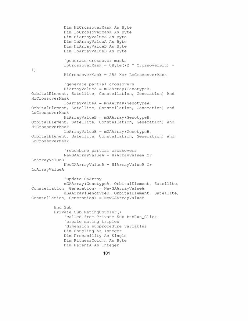
101

Dim HiCrossoverMask As Byte Dim LoCrossoverMask As Byte Dim HiArrayValueA As Byte Dim LoArrayValueA As Byte Dim HiArrayValueB As Byte Dim LoArrayValueB As Byte 'generate crossover masks LoCrossoverMask = CByte((2 ^ CrossoverBit) -

1) HiCrossoverMask = 255 Xor LoCrossoverMask 'generate partial crossovers HiArrayValueA = mGAArray(GenotypeA,

OrbitalElement, Satellite, Constellation, Generation) And HiCrossoverMask

LoArrayValueA = mGAArray(GenotypeA, OrbitalElement, Satellite, Constellation, Generation) And LoCrossoverMask

HiArrayValueB = mGAArray(GenotypeB, OrbitalElement, Satellite, Constellation, Generation) And HiCrossoverMask

LoArrayValueB = mGAArray(GenotypeB, OrbitalElement, Satellite, Constellation, Generation) And LoCrossoverMask

'recombine partial crossovers NewGAArrayValueA = HiArrayValueA Or

LoArrayValueB NewGAArrayValueB = HiArrayValueB Or

LoArrayValueA 'update GAArray mGAArray(GenotypeA, OrbitalElement, Satellite,

Constellation, Generation) = NewGAArrayValueA mGAArray(GenotypeB, OrbitalElement, Satellite,

Constellation, Generation) = NewGAArrayValueB End Sub Private Sub MatingCoupler() 'called from Private Sub btnRun_Click 'create mating triples 'dimension subprocedure variables Dim Coupling As Integer Dim Probability As Single Dim FitnessColumn As Byte Dim ParentA As Integer

102

Dim ParentB As Integer Dim ParentC As Integer 'roulette wheel selection of parents 'requires the fitnesses to be scaled For Coupling = 0 To CInt((mTotalConstellations

/ 3) - 1) Probability = Rnd() For FitnessColumn = 0 To

(mTotalConstellations - 1) If Probability < mFitnessArray(5,

FitnessColumn, mCurrentGeneration - 1) Then ParentA = FitnessColumn End If Next Probability = Rnd() For FitnessColumn = 0 To


FitnessColumn, mCurrentGeneration - 1) Then ParentB = FitnessColumn End If Next Probability = Rnd() For FitnessColumn = 0 To


FitnessColumn, mCurrentGeneration - 1) Then ParentC = FitnessColumn End If Next Call CreateOffspring(ParentA, ParentB,

ParentC, Coupling) Next Coupling End Sub Private Sub CreateOffspring(ByVal ParentA As

Integer, ByVal ParentB As Integer, ByVal ParentC As Integer, ByVal Coupling As Integer)

'called from Private Sub MatingCoupler 'create next generation 'dimension subprocedure variables Dim Satellite As Integer Dim OrbitalElement As Integer 'create offspring 1

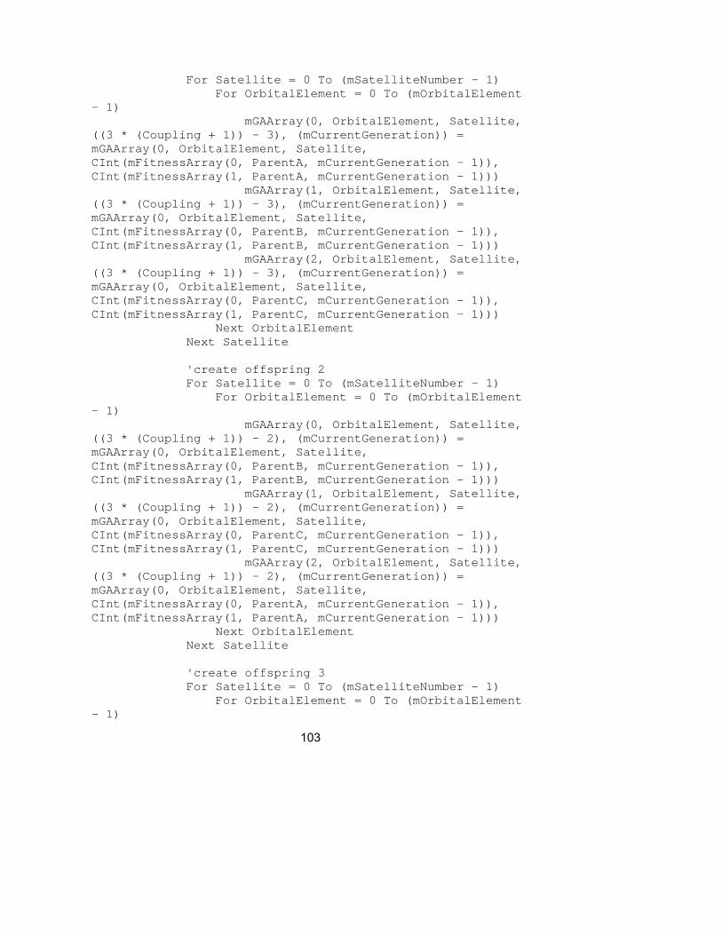
103

For Satellite = 0 To (mSatelliteNumber - 1) For OrbitalElement = 0 To (mOrbitalElement

- 1) mGAArray(0, OrbitalElement, Satellite,

((3 * (Coupling + 1)) - 3), (mCurrentGeneration)) = mGAArray(0, OrbitalElement, Satellite, CInt(mFitnessArray(0, ParentA, mCurrentGeneration - 1)), CInt(mFitnessArray(1, ParentA, mCurrentGeneration - 1)))

mGAArray(1, OrbitalElement, Satellite, ((3 * (Coupling + 1)) - 3), (mCurrentGeneration)) = mGAArray(0, OrbitalElement, Satellite, CInt(mFitnessArray(0, ParentB, mCurrentGeneration - 1)), CInt(mFitnessArray(1, ParentB, mCurrentGeneration - 1)))

mGAArray(2, OrbitalElement, Satellite, ((3 * (Coupling + 1)) - 3), (mCurrentGeneration)) = mGAArray(0, OrbitalElement, Satellite, CInt(mFitnessArray(0, ParentC, mCurrentGeneration - 1)), CInt(mFitnessArray(1, ParentC, mCurrentGeneration - 1)))

Next OrbitalElement Next Satellite 'create offspring 2 For Satellite = 0 To (mSatelliteNumber - 1) For OrbitalElement = 0 To (mOrbitalElement

- 1) mGAArray(0, OrbitalElement, Satellite,

((3 * (Coupling + 1)) - 2), (mCurrentGeneration)) = mGAArray(0, OrbitalElement, Satellite, CInt(mFitnessArray(0, ParentB, mCurrentGeneration - 1)), CInt(mFitnessArray(1, ParentB, mCurrentGeneration - 1)))


mGAArray(2, OrbitalElement, Satellite, ((3 * (Coupling + 1)) - 2), (mCurrentGeneration)) = mGAArray(0, OrbitalElement, Satellite, CInt(mFitnessArray(0, ParentA, mCurrentGeneration - 1)), CInt(mFitnessArray(1, ParentA, mCurrentGeneration - 1)))

Next OrbitalElement Next Satellite 'create offspring 3 For Satellite = 0 To (mSatelliteNumber - 1) For OrbitalElement = 0 To (mOrbitalElement

- 1)

104


mGAArray(1, OrbitalElement, Satellite, ((3 * (Coupling + 1)) - 1), (mCurrentGeneration)) = mGAArray(0, OrbitalElement, Satellite, CInt(mFitnessArray(0, ParentA, mCurrentGeneration - 1)), CInt(mFitnessArray(1, ParentA, mCurrentGeneration - 1)))

mGAArray(2, OrbitalElement, Satellite, ((3 * (Coupling + 1)) - 1), (mCurrentGeneration)) = mGAArray(0, OrbitalElement, Satellite, CInt(mFitnessArray(0, ParentB, mCurrentGeneration - 1)), CInt(mFitnessArray(1, ParentB, mCurrentGeneration - 1)))

Next OrbitalElement Next Satellite End Sub Private Sub MutationEngine() 'called from Private Sub btnRun_Click 'determine if mutation occurs 'dimension subprocedure variables Dim Constellation As Integer Dim Satellite As Integer Dim OrbitalElement As Integer Dim Genotype As Integer Dim Bit As Integer 'loop through possible mutation locations to

determine where mutation occurs For Constellation = 0 To (mTotalConstellations



(mOrbitalElement - 1) For Genotype = 0 To 2 For Bit = 1 To 8 If Rnd() <

mMutationProbability Then Call

Mutation(Genotype, OrbitalElement, Satellite, Constellation, mCurrentGeneration, Bit)

End If Next Bit Next Genotype

105

Next OrbitalElement Next Satellite Next Constellation End Sub Private Sub Mutation(ByVal Genotype As Integer,

ByVal OrbitalElement As Integer, ByVal Satellite As Integer, ByVal Constellation As Integer, ByVal Generation As Integer, ByVal MutationBit As Integer)

'called from Private Sub MutationEngine 'mutate given bit 'mutation is a bit flip 'dimension variables Dim MutationMask As Byte 'create mutation mask MutationMask = CInt(2 ^ (MutationBit - 1)) 'update GAArray mGAArray(Genotype, OrbitalElement, Satellite,

Constellation, Generation) = mGAArray(Genotype, OrbitalElement, Satellite, Constellation, Generation) Xor MutationMask

End Sub Private Sub CopyFitnessArray() 'copy previous generation fitness scores into

current array for comparison. Dim FitnessColumn As Integer Dim FitnessRow As Integer For FitnessColumn = 0 To (mTotalConstellations

- 1) For FitnessRow = 0 To 5 mFitnessArray(FitnessRow,

FitnessColumn, mCurrentGeneration) = mFitnessArray(FitnessRow, FitnessColumn, mCurrentGeneration - 1)

Next FitnessRow Next FitnessColumn End Sub Private Function SemiMajorAxis(ByVal ArrayValue As

Byte) As Single 'return a scaled altitude value to the fitness

function

106

SemiMajorAxis = 1000 * (6378.1363 + (MinSemiMajorAxis + ((MaxSemiMajorAxis - MinSemiMajorAxis) * (ArrayValue / 255))))

End Function Private Function Inclination(ByVal ArrayValue As

Byte) As Single 'return a scaled inclination to the fitness

function Inclination = MinInclination +

((MaxInclination - MinInclination) * (ArrayValue / 255)) End Function Private Function RightAscension(ByVal ArrayValue

As Byte, ByVal Satellite As Integer) As Single 'return a scaled right ascension to the

fitness function If Satellite = 0 Then mPreviousRightAscension = 0 RightAscension = MinRightAscension +

((MaxRightAscension - MinRightAscension) * (ArrayValue / 255))

ElseIf mPreviousRightAscension + (MinRightAscension + ((MaxRightAscension - MinRightAscension) * (ArrayValue / 255))) > 360 Then

RightAscension = (mPreviousRightAscension + (MinRightAscension + ((MaxRightAscension - MinRightAscension) * (ArrayValue / 255)))) - 360

Else RightAscension = mPreviousRightAscension +

(MinRightAscension + ((MaxRightAscension - MinRightAscension) * (ArrayValue / 255)))

End If mPreviousRightAscension = RightAscension End Function Private Function Anomaly(ByVal ArrayValue As Byte,

ByVal Satellite As Integer) As Single 'return a scaled anomaly to the fitness

function If Satellite = 0 Then mPreviousAnomaly = 0 Anomaly = MinAnomaly + ((MaxAnomaly -

MinAnomaly) * (ArrayValue / 255)) ElseIf mPreviousAnomaly + (MinAnomaly +

((MaxAnomaly - MinAnomaly) * (ArrayValue / 255))) > 360 Then

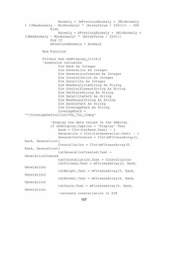
107

Anomaly = (mPreviousAnomaly + (MinAnomaly + ((MaxAnomaly - MinAnomaly) * (ArrayValue / 255)))) - 360

Else Anomaly = mPreviousAnomaly + (MinAnomaly +

((MaxAnomaly - MinAnomaly) * (ArrayValue / 255))) End If mPreviousAnomaly = Anomaly End Function Private Sub cmdDisplay_Click() 'dimension variables Dim Rank As Integer Dim Generation As Integer Dim GenerationCreated As Integer Dim Constellation As Integer Dim Satellite As Integer Dim NewSatelliteString As String Dim OrbitalElementString As String Dim SetStateString As String Dim SatellitePath As String Dim NewSensorString As String Dim SensorPath As String Dim CoveragePath As String CoveragePath =

"*/CoverageDefinition/55s_75n_10deg" 'display the data values in the GAArray If cmdDisplay.Caption = "Display" Then Rank = CInt(txtRank.Text) - 1 Generation = CInt(txtGeneration.Text) - 1 GenerationCreated = CInt(mFitnessArray(1,

Rank, Generation)) Constellation = CInt(mFitnessArray(0,

Rank, Generation)) txtGenerationCreated.Text =

GenerationCreated txtConstellation.Text = Constellation txtFitness.Text = mFitnessArray(2, Rank,

Generation) txtWeight.Text = mFitnessArray(3, Rank,

Generation) txtNormal.Text = mFitnessArray(4, Rank,

Generation) txtScale.Text = mFitnessArray(5, Rank,

Generation) 'recreate constellation in STK

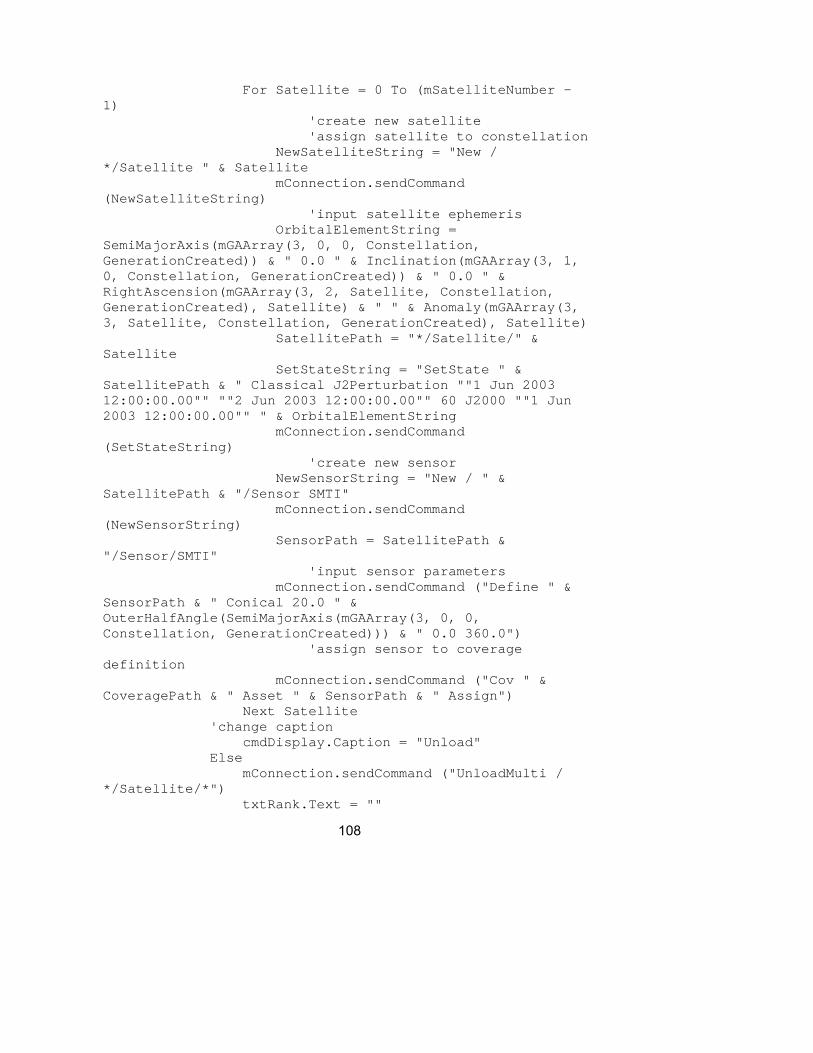
108

For Satellite = 0 To (mSatelliteNumber - 1)

'create new satellite 'assign satellite to constellation NewSatelliteString = "New /

*/Satellite " & Satellite mConnection.sendCommand

(NewSatelliteString) 'input satellite ephemeris OrbitalElementString =

SemiMajorAxis(mGAArray(3, 0, 0, Constellation, GenerationCreated)) & " 0.0 " & Inclination(mGAArray(3, 1, 0, Constellation, GenerationCreated)) & " 0.0 " & RightAscension(mGAArray(3, 2, Satellite, Constellation, GenerationCreated), Satellite) & " " & Anomaly(mGAArray(3, 3, Satellite, Constellation, GenerationCreated), Satellite)

SatellitePath = "*/Satellite/" & Satellite

SetStateString = "SetState " & SatellitePath & " Classical J2Perturbation ""1 Jun 2003 12:00:00.00"" ""2 Jun 2003 12:00:00.00"" 60 J2000 ""1 Jun 2003 12:00:00.00"" " & OrbitalElementString

mConnection.sendCommand (SetStateString)

'create new sensor NewSensorString = "New / " &

SatellitePath & "/Sensor SMTI" mConnection.sendCommand

(NewSensorString) SensorPath = SatellitePath &

"/Sensor/SMTI" 'input sensor parameters mConnection.sendCommand ("Define " &

SensorPath & " Conical 20.0 " & OuterHalfAngle(SemiMajorAxis(mGAArray(3, 0, 0, Constellation, GenerationCreated))) & " 0.0 360.0")

'assign sensor to coverage definition

mConnection.sendCommand ("Cov " & CoveragePath & " Asset " & SensorPath & " Assign")

Next Satellite 'change caption cmdDisplay.Caption = "Unload" Else mConnection.sendCommand ("UnloadMulti /

*/Satellite/*") txtRank.Text = ""

109

txtGeneration.Text = "" cmdDisplay.Caption = "Display" End If End Sub Private Function OuterHalfAngle(ByVal

SemiMajorAxis As Single) As Single 'calculate outer half angle for given semi major

axis Const pi As Single = 3.14159265358979 Dim x As Single Dim Radians As Single x = Cos(pi / 30) * (6378.1363 / (SemiMajorAxis /

1000)) Radians = Atn(x / Sqr(-x * x + 1)) OuterHalfAngle = Radians * (180 / pi) End Function Private Sub ReadData() Dim Constellation As Integer Dim Satellite As Integer Dim OrbitalElement As Integer Dim Genotype As Integer Dim Data As Integer Dim Position As Integer Position = 1 Open "C:\Documents and Settings\Douglas J.

Pegher\My Documents\Thesis\VB6\COMPGAvbyte\data\gabytedata.txt" For Random Access Read As #1

' Read the contents of the file. For Constellation = 0 To (mTotalConstellations -

1) For Satellite = 0 To (mSatelliteNumber - 1) For OrbitalElement = 0 To (mOrbitalElement

- 1) For Genotype = 0 To 2 Get #1, Position, Data mGAArray(Genotype, OrbitalElement,

Satellite, Constellation, 0) = Data Position = Position + 1 Next Genotype Next OrbitalElement Next Satellite Next Constellation Close #1 End Sub Private Sub WriteData()

110

Dim Constellation As Integer Dim Satellite As Integer Dim OrbitalElement As Integer Dim Genotype As Integer Dim Data As Integer Dim Position As Integer Position = 1 Open "C:\Documents and Settings\Douglas J.

Pegher\My Documents\Thesis\VB6\COMPGAvbyte\data\gabytedata.txt" For Random Access Write As #1

For Constellation = 0 To (mTotalConstellations



(mOrbitalElement - 1) For Genotype = 0 To 2 Data = (mGAArray(Genotype,

OrbitalElement, Satellite, mFitnessArray(0, Constellation, (mLastGeneration - 1)), mFitnessArray(1, Constellation, (mLastGeneration - 1))))

Put #1, Position, Data Position = Position + 1 Next Genotype Next OrbitalElement Next Satellite Next Constellation Close #1 End Sub Private Sub WriteFitness() Dim fso, txtfile Set fso =

CreateObject("Scripting.FileSystemObject") Set txtfile = fso.OpenTextFile("C:\Documents and

Settings\Douglas J. Pegher\My Documents\Thesis\VB6\COMPGAvbyte\data\fitnessbytedata.txt", 8)

' Write a line with a newline character. txtfile.WriteLine (mFitnessArray(2, 0, 19)) txtfile.Close End Sub

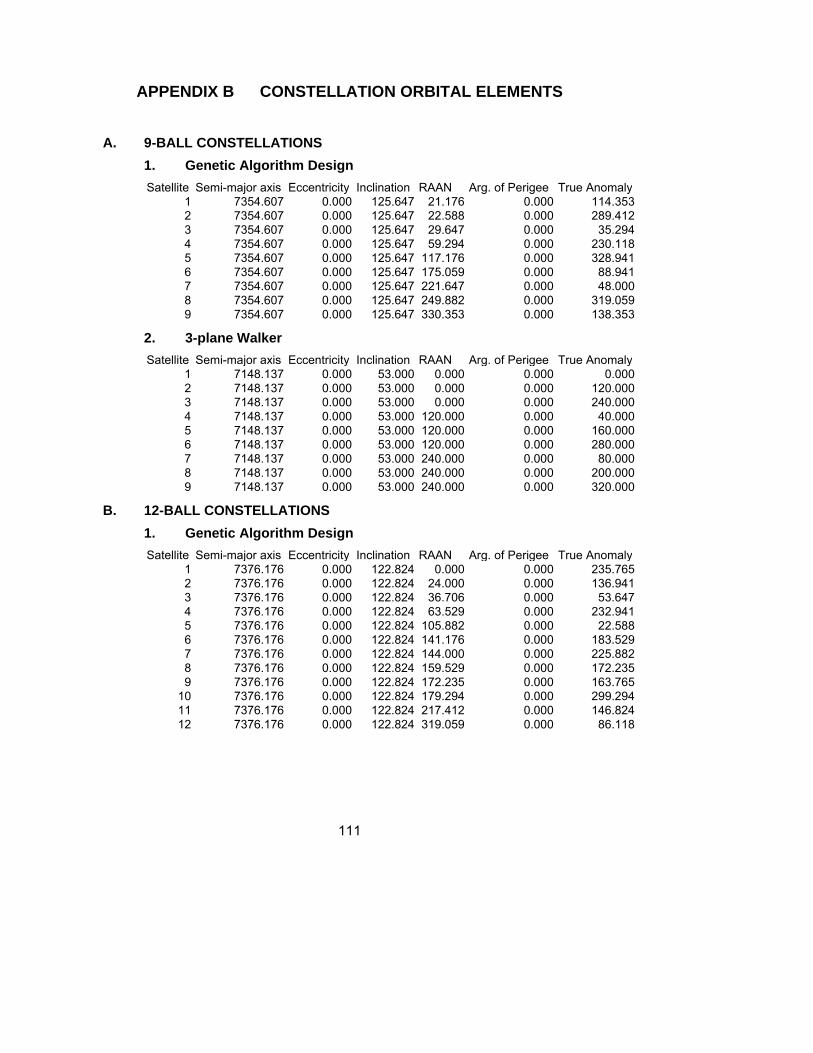
111

APPENDIX B CONSTELLATION ORBITAL ELEMENTS

A. 9-BALL CONSTELLATIONS 1. Genetic Algorithm Design Satellite Semi-major axis Eccentricity Inclination RAAN Arg. of Perigee True Anomaly

1 7354.607 0.000 125.647 21.176 0.000 114.3532 7354.607 0.000 125.647 22.588 0.000 289.4123 7354.607 0.000 125.647 29.647 0.000 35.2944 7354.607 0.000 125.647 59.294 0.000 230.1185 7354.607 0.000 125.647 117.176 0.000 328.9416 7354.607 0.000 125.647 175.059 0.000 88.9417 7354.607 0.000 125.647 221.647 0.000 48.0008 7354.607 0.000 125.647 249.882 0.000 319.0599 7354.607 0.000 125.647 330.353 0.000 138.353

2. 3-plane Walker Satellite Semi-major axis Eccentricity Inclination RAAN Arg. of Perigee True Anomaly

1 7148.137 0.000 53.000 0.000 0.000 0.0002 7148.137 0.000 53.000 0.000 0.000 120.0003 7148.137 0.000 53.000 0.000 0.000 240.0004 7148.137 0.000 53.000 120.000 0.000 40.0005 7148.137 0.000 53.000 120.000 0.000 160.0006 7148.137 0.000 53.000 120.000 0.000 280.0007 7148.137 0.000 53.000 240.000 0.000 80.0008 7148.137 0.000 53.000 240.000 0.000 200.0009 7148.137 0.000 53.000 240.000 0.000 320.000

B. 12-BALL CONSTELLATIONS 1. Genetic Algorithm Design Satellite Semi-major axis Eccentricity Inclination RAAN Arg. of Perigee True Anomaly

1 7376.176 0.000 122.824 0.000 0.000 235.7652 7376.176 0.000 122.824 24.000 0.000 136.9413 7376.176 0.000 122.824 36.706 0.000 53.6474 7376.176 0.000 122.824 63.529 0.000 232.9415 7376.176 0.000 122.824 105.882 0.000 22.5886 7376.176 0.000 122.824 141.176 0.000 183.5297 7376.176 0.000 122.824 144.000 0.000 225.8828 7376.176 0.000 122.824 159.529 0.000 172.2359 7376.176 0.000 122.824 172.235 0.000 163.765

10 7376.176 0.000 122.824 179.294 0.000 299.29411 7376.176 0.000 122.824 217.412 0.000 146.82412 7376.176 0.000 122.824 319.059 0.000 86.118

112


1 7148.137 0.000 53.000 0.000 0.000 0.0002 7148.137 0.000 53.000 0.000 0.000 120.0003 7148.137 0.000 53.000 0.000 0.000 240.0004 7148.137 0.000 53.000 90.000 0.000 30.0005 7148.137 0.000 53.000 90.000 0.000 150.0006 7148.137 0.000 53.000 90.000 0.000 270.0007 7148.137 0.000 53.000 180.000 0.000 60.0008 7148.137 0.000 53.000 180.000 0.000 180.0009 7148.137 0.000 53.000 180.000 0.000 300.000

10 7148.137 0.000 53.000 270.000 0.000 90.00011 7148.137 0.000 53.000 270.000 0.000 210.00012 7148.137 0.000 53.000 270.000 0.000 330.000

C. 18-BALL CONSTELLATIONS 1. Genetic Algorithm Design Satellite Semi-major axis Eccentricity Inclination RAAN Arg. of Perigee True Anomaly

1 7378.136 0.000 121.412 1.412 0.000 120.0002 7378.136 0.000 121.412 14.118 0.000 149.6473 7378.136 0.000 121.412 21.176 0.000 203.2944 7378.136 0.000 121.412 117.176 0.000 317.6475 7378.136 0.000 121.412 118.588 0.000 83.2946 7378.136 0.000 121.412 131.294 0.000 11.2947 7378.136 0.000 121.412 131.294 0.000 73.4128 7378.136 0.000 121.412 149.647 0.000 155.2949 7378.136 0.000 121.412 187.765 0.000 278.118

10 7378.136 0.000 121.412 196.235 0.000 165.17611 7378.136 0.000 121.412 204.706 0.000 57.88212 7378.136 0.000 121.412 206.118 0.000 125.64713 7378.136 0.000 121.412 216.000 0.000 240.00014 7378.136 0.000 121.412 279.529 0.000 21.17615 7378.136 0.000 121.412 285.176 0.000 272.47116 7378.136 0.000 121.412 293.647 0.000 271.05917 7378.136 0.000 121.412 330.353 0.000 21.17618 7378.136 0.000 121.412 350.118 0.000 59.294

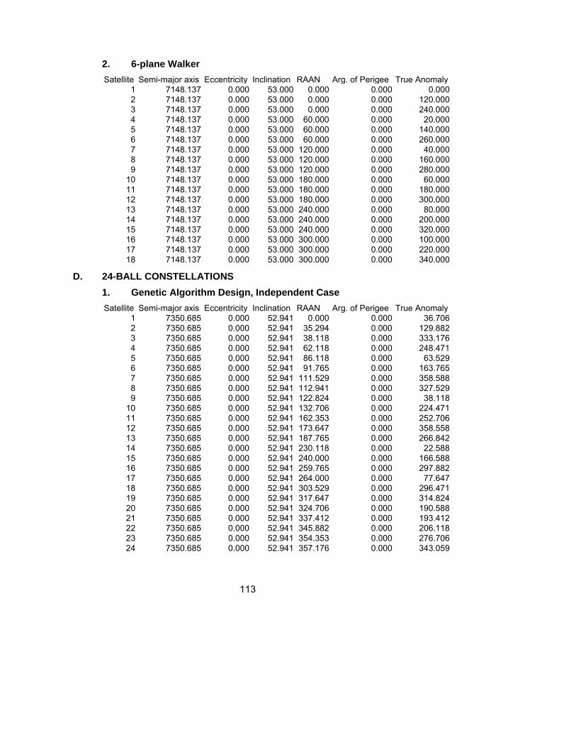
113


1 7148.137 0.000 53.000 0.000 0.000 0.0002 7148.137 0.000 53.000 0.000 0.000 120.0003 7148.137 0.000 53.000 0.000 0.000 240.0004 7148.137 0.000 53.000 60.000 0.000 20.0005 7148.137 0.000 53.000 60.000 0.000 140.0006 7148.137 0.000 53.000 60.000 0.000 260.0007 7148.137 0.000 53.000 120.000 0.000 40.0008 7148.137 0.000 53.000 120.000 0.000 160.0009 7148.137 0.000 53.000 120.000 0.000 280.000

10 7148.137 0.000 53.000 180.000 0.000 60.00011 7148.137 0.000 53.000 180.000 0.000 180.00012 7148.137 0.000 53.000 180.000 0.000 300.00013 7148.137 0.000 53.000 240.000 0.000 80.00014 7148.137 0.000 53.000 240.000 0.000 200.00015 7148.137 0.000 53.000 240.000 0.000 320.00016 7148.137 0.000 53.000 300.000 0.000 100.00017 7148.137 0.000 53.000 300.000 0.000 220.00018 7148.137 0.000 53.000 300.000 0.000 340.000

D. 24-BALL CONSTELLATIONS 1. Genetic Algorithm Design, Independent Case Satellite Semi-major axis Eccentricity Inclination RAAN Arg. of Perigee True Anomaly

1 7350.685 0.000 52.941 0.000 0.000 36.7062 7350.685 0.000 52.941 35.294 0.000 129.8823 7350.685 0.000 52.941 38.118 0.000 333.1764 7350.685 0.000 52.941 62.118 0.000 248.4715 7350.685 0.000 52.941 86.118 0.000 63.5296 7350.685 0.000 52.941 91.765 0.000 163.7657 7350.685 0.000 52.941 111.529 0.000 358.5888 7350.685 0.000 52.941 112.941 0.000 327.5299 7350.685 0.000 52.941 122.824 0.000 38.118

10 7350.685 0.000 52.941 132.706 0.000 224.47111 7350.685 0.000 52.941 162.353 0.000 252.70612 7350.685 0.000 52.941 173.647 0.000 358.55813 7350.685 0.000 52.941 187.765 0.000 266.84214 7350.685 0.000 52.941 230.118 0.000 22.58815 7350.685 0.000 52.941 240.000 0.000 166.58816 7350.685 0.000 52.941 259.765 0.000 297.88217 7350.685 0.000 52.941 264.000 0.000 77.64718 7350.685 0.000 52.941 303.529 0.000 296.47119 7350.685 0.000 52.941 317.647 0.000 314.82420 7350.685 0.000 52.941 324.706 0.000 190.58821 7350.685 0.000 52.941 337.412 0.000 193.41222 7350.685 0.000 52.941 345.882 0.000 206.11823 7350.685 0.000 52.941 354.353 0.000 276.70624 7350.685 0.000 52.941 357.176 0.000 343.059

114

2. Genetic Algorithm Design, Dependent Case Satellite Semi-major axis Eccentricity Inclination RAAN Arg. of Perigee True Anomaly

1 7352.791 0.000 62.618 3.038 0.000 349.6672 7352.791 0.000 62.618 11.657 0.000 15.6503 7352.791 0.000 62.618 25.813 0.000 274.4984 7352.791 0.000 62.618 50.065 0.000 13.2995 7352.791 0.000 62.618 50.758 0.000 339.9226 7352.791 0.000 62.618 84.777 0.000 62.7497 7352.791 0.000 62.618 95.269 0.000 271.7958 7352.791 0.000 62.618 112.386 0.000 159.2889 7352.791 0.000 62.618 125.620 0.000 215.918

10 7352.791 0.000 62.618 151.174 0.000 345.47011 7352.791 0.000 62.618 182.892 0.000 41.85912 7352.791 0.000 62.618 188.506 0.000 261.78113 7352.791 0.000 62.618 202.602 0.000 124.68614 7352.791 0.000 62.618 204.019 0.000 150.30615 7352.791 0.000 62.618 205.316 0.000 47.96716 7352.791 0.000 62.618 208.941 0.000 3.25217 7352.791 0.000 62.618 227.179 0.000 182.42018 7352.791 0.000 62.618 248.443 0.000 294.39419 7352.791 0.000 62.618 262.204 0.000 18.83120 7352.791 0.000 62.618 285.836 0.000 279.12321 7352.791 0.000 62.618 299.948 0.000 48.46722 7352.791 0.000 62.618 301.371 0.000 206.27723 7352.791 0.000 62.618 332.133 0.000 315.23524 7352.791 0.000 62.618 335.434 0.000 344.690

115


1 7148.137 0.000 53.000 0.000 0.000 0.0002 7148.137 0.000 53.000 0.000 0.000 60.0003 7148.137 0.000 53.000 0.000 0.000 120.0004 7148.137 0.000 53.000 0.000 0.000 180.0005 7148.137 0.000 53.000 0.000 0.000 240.0006 7148.137 0.000 53.000 0.000 0.000 300.0007 7148.137 0.000 53.000 90.000 0.000 15.0008 7148.137 0.000 53.000 90.000 0.000 75.0009 7148.137 0.000 53.000 90.000 0.000 135.000

10 7148.137 0.000 53.000 90.000 0.000 195.00011 7148.137 0.000 53.000 90.000 0.000 255.00012 7148.137 0.000 53.000 90.000 0.000 315.00013 7148.137 0.000 53.000 180.000 0.000 30.00014 7148.137 0.000 53.000 180.000 0.000 90.00015 7148.137 0.000 53.000 180.000 0.000 150.00016 7148.137 0.000 53.000 180.000 0.000 210.00017 7148.137 0.000 53.000 180.000 0.000 270.00018 7148.137 0.000 53.000 180.000 0.000 330.00019 7148.137 0.000 53.000 270.000 0.000 45.00020 7148.137 0.000 53.000 270.000 0.000 105.00021 7148.137 0.000 53.000 270.000 0.000 165.00022 7148.137 0.000 53.000 270.000 0.000 225.00023 7148.137 0.000 53.000 270.000 0.000 285.00024 7148.137 0.000 53.000 270.000 0.000 345.000

116


1 7148.137 0.000 53.000 0.000 0.000 90.0002 7148.137 0.000 53.000 0.000 0.000 180.0003 7148.137 0.000 53.000 0.000 0.000 270.0004 7148.137 0.000 53.000 0.000 0.000 360.0005 7148.137 0.000 53.000 60.000 0.000 15.0006 7148.137 0.000 53.000 60.000 0.000 105.0007 7148.137 0.000 53.000 60.000 0.000 195.0008 7148.137 0.000 53.000 60.000 0.000 285.0009 7148.137 0.000 53.000 120.000 0.000 30.000

10 7148.137 0.000 53.000 120.000 0.000 120.00011 7148.137 0.000 53.000 120.000 0.000 210.00012 7148.137 0.000 53.000 120.000 0.000 300.00013 7148.137 0.000 53.000 180.000 0.000 45.00014 7148.137 0.000 53.000 180.000 0.000 135.00015 7148.137 0.000 53.000 180.000 0.000 255.00016 7148.137 0.000 53.000 180.000 0.000 315.00017 7148.137 0.000 53.000 240.000 0.000 60.00018 7148.137 0.000 53.000 240.000 0.000 150.00019 7148.137 0.000 53.000 240.000 0.000 240.00020 7148.137 0.000 53.000 240.000 0.000 330.00021 7148.137 0.000 53.000 300.000 0.000 75.00022 7148.137 0.000 53.000 300.000 0.000 165.00023 7148.137 0.000 53.000 300.000 0.000 255.00024 7148.137 0.000 53.000 300.000 0.000 345.000

117

5. 8-plane Walker, Discoverer II Satellite Semi-major axis Eccentricity Inclination RAAN Arg. of Perigee True Anomaly

1 7148.137 0.000 53.000 0.000 0.000 0.0002 7148.137 0.000 53.000 0.000 0.000 120.0003 7148.137 0.000 53.000 0.000 0.000 240.0004 7148.137 0.000 53.000 45.000 0.000 15.0005 7148.137 0.000 53.000 45.000 0.000 135.0006 7148.137 0.000 53.000 45.000 0.000 255.0007 7148.137 0.000 53.000 90.000 0.000 30.0008 7148.137 0.000 53.000 90.000 0.000 150.0009 7148.137 0.000 53.000 90.000 0.000 270.000

10 7148.137 0.000 53.000 135.000 0.000 45.00011 7148.137 0.000 53.000 135.000 0.000 165.00012 7148.137 0.000 53.000 135.000 0.000 285.00013 7148.137 0.000 53.000 180.000 0.000 60.00014 7148.137 0.000 53.000 180.000 0.000 180.00015 7148.137 0.000 53.000 180.000 0.000 300.00016 7148.137 0.000 53.000 225.000 0.000 75.00017 7148.137 0.000 53.000 225.000 0.000 195.00018 7148.137 0.000 53.000 225.000 0.000 315.00019 7148.137 0.000 53.000 270.000 0.000 90.00020 7148.137 0.000 53.000 270.000 0.000 210.00021 7148.137 0.000 53.000 270.000 0.000 330.00022 7148.137 0.000 53.000 315.000 0.000 105.00023 7148.137 0.000 53.000 315.000 0.000 225.00024 7148.137 0.000 53.000 315.000 0.000 345.000

118


1 7148.137 0.000 53.000 0.000 0.000 0.0002 7148.137 0.000 53.000 0.000 0.000 180.0003 7148.137 0.000 53.000 30.000 0.000 15.0004 7148.137 0.000 53.000 30.000 0.000 195.0005 7148.137 0.000 53.000 60.000 0.000 30.0006 7148.137 0.000 53.000 60.000 0.000 210.0007 7148.137 0.000 53.000 90.000 0.000 45.0008 7148.137 0.000 53.000 90.000 0.000 225.0009 7148.137 0.000 53.000 120.000 0.000 60.000

10 7148.137 0.000 53.000 120.000 0.000 240.00011 7148.137 0.000 53.000 150.000 0.000 75.00012 7148.137 0.000 53.000 150.000 0.000 255.00013 7148.137 0.000 53.000 180.000 0.000 90.00014 7148.137 0.000 53.000 180.000 0.000 270.00015 7148.137 0.000 53.000 210.000 0.000 105.00016 7148.137 0.000 53.000 210.000 0.000 285.00017 7148.137 0.000 53.000 240.000 0.000 120.00018 7148.137 0.000 53.000 240.000 0.000 300.00019 7148.137 0.000 53.000 270.000 0.000 135.00020 7148.137 0.000 53.000 270.000 0.000 315.00021 7148.137 0.000 53.000 300.000 0.000 150.00022 7148.137 0.000 53.000 300.000 0.000 330.00023 7148.137 0.000 53.000 330.000 0.000 165.00024 7148.137 0.000 53.000 330.000 0.000 345.000

119

APPENDIX C CONSTELLATION FITNESS CALCULATIONS

A. 9-BALL CONSTELLATIONS 1. Genetic Algorithm Design Latitude Avg Gap (s) Max Gap (s) Percent Coverage Weight SubTotal

55 S 919.509 3705.992 46.812 0.002 0.00145 S 781.436 3075.419 48.362 0.007 0.00435 S 755.448 3334.331 47.534 0.027 0.01625 S 1644.733 5243.500 36.817 0.068 0.04815 S 1741.932 4686.921 32.911 0.070 0.0525 S 2047.105 5347.022 28.344 0.075 0.0615 N 2123.327 5255.546 27.844 0.074 0.06015 N 1865.481 4496.814 31.964 0.086 0.06525 N 1430.228 4271.515 36.826 0.112 0.07835 N 814.251 3353.300 47.396 0.116 0.06645 N 752.109 3084.668 50.229 0.120 0.06555 N 858.545 3707.625 46.371 0.109 0.06465 N 1152.072 3726.425 40.066 0.108 0.07175 N 2026.571 4221.155 21.518 0.026 0.022

Overall Fitness 0.673 2. 3-plane Walker Latitude Avg Gap (s) Max Gap (s) Percent Coverage Weight SubTotal

55 S 782.582 1351.709 38.089 0.002 0.00145 S 836.317 1367.876 36.631 0.007 0.00535 S 964.183 1669.642 33.002 0.027 0.01925 S 4578.149 11902.070 26.467 0.068 0.06315 S 3241.265 9431.575 27.775 0.070 0.0615 S 1415.000 5034.016 25.792 0.075 0.0625 N 1684.521 5085.822 25.914 0.074 0.06115 N 2914.770 9430.366 27.755 0.086 0.07425 N 5286.915 11888.390 26.910 0.112 0.10435 N 958.828 1670.349 32.586 0.116 0.08145 N 840.448 1367.978 36.803 0.120 0.07955 N 786.705 1651.903 38.056 0.109 0.07165 N 1021.122 1711.516 29.274 0.108 0.08075 N 9916.763 16956.361 6.153 0.026 0.033

Overall Fitness 0.793

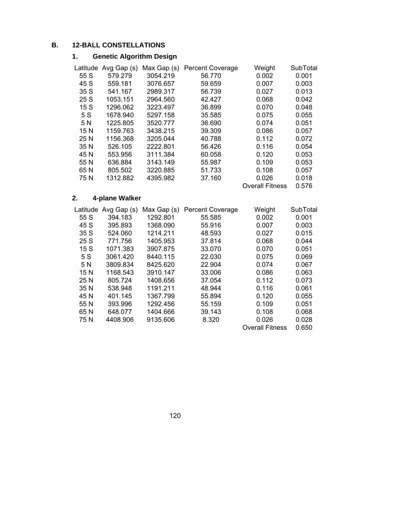
120

B. 12-BALL CONSTELLATIONS 1. Genetic Algorithm Design Latitude Avg Gap (s) Max Gap (s) Percent Coverage Weight SubTotal

55 S 579.279 3054.219 56.770 0.002 0.00145 S 559.181 3076.657 59.659 0.007 0.00335 S 541.167 2989.317 56.739 0.027 0.01325 S 1053.151 2964.560 42.427 0.068 0.04215 S 1296.062 3223.497 36.899 0.070 0.0485 S 1678.940 5297.158 35.585 0.075 0.0555 N 1225.805 3520.777 36.690 0.074 0.05115 N 1159.763 3438.215 39.309 0.086 0.05725 N 1156.368 3205.044 40.788 0.112 0.07235 N 526.105 2222.801 56.426 0.116 0.05445 N 553.956 3111.384 60.058 0.120 0.05355 N 636.884 3143.149 55.987 0.109 0.05365 N 805.502 3220.885 51.733 0.108 0.05775 N 1312.882 4395.982 37.160 0.026 0.018


55 S 394.183 1292.801 55.585 0.002 0.00145 S 395.893 1368.090 55.916 0.007 0.00335 S 524.060 1214.211 48.593 0.027 0.01525 S 771.756 1405.953 37.814 0.068 0.04415 S 1071.383 3907.875 33.070 0.070 0.0515 S 3061.420 8440.115 22.030 0.075 0.0695 N 3809.834 8425.620 22.904 0.074 0.06715 N 1168.543 3910.147 33.006 0.086 0.06325 N 805.724 1408.656 37.054 0.112 0.07335 N 538.948 1191.211 48.944 0.116 0.06145 N 401.145 1367.799 55.894 0.120 0.05555 N 393.996 1292.456 55.159 0.109 0.05165 N 648.077 1404.666 39.143 0.108 0.06875 N 4408.906 9135.606 8.320 0.026 0.028


121

C. 18-BALL CONSTELLATIONS 1. Genetic Algorithm Design Latitude Avg Gap (s) Max Gap (s) Percent Coverage Weight SubTotal

55 S 118.477 1127.385 79.441 0.002 0.00045 S 157.996 1573.414 78.347 0.007 0.00235 S 184.171 1610.249 74.338 0.027 0.00825 S 570.950 3459.280 59.662 0.068 0.03115 S 884.022 4608.824 51.893 0.070 0.0385 S 1360.776 6551.061 50.015 0.075 0.0455 N 784.243 3816.616 51.898 0.074 0.03915 N 761.982 3783.120 53.260 0.086 0.04525 N 561.826 3319.595 58.549 0.112 0.05235 N 196.870 1602.849 73.356 0.116 0.03345 N 126.280 1281.195 79.720 0.120 0.02655 N 122.982 1153.650 78.120 0.109 0.02565 N 187.430 1406.318 73.263 0.108 0.03175 N 453.192 2600.306 58.152 0.026 0.012


55 S 61.586 394.774 76.363 0.002 0.00045 S 74.406 299.074 73.357 0.007 0.00235 S 132.860 580.481 65.589 0.027 0.01025 S 411.193 1177.516 53.693 0.068 0.03315 S 510.161 1361.840 49.621 0.070 0.0375 S 964.934 2545.831 33.608 0.075 0.0535 N 926.677 2545.482 33.872 0.074 0.05215 N 509.759 1362.448 49.739 0.086 0.04525 N 421.954 1155.045 53.474 0.112 0.05435 N 133.069 580.747 65.571 0.116 0.04145 N 74.403 299.427 73.360 0.120 0.03255 N 61.310 394.724 76.276 0.109 0.02665 N 219.857 745.152 58.540 0.108 0.04675 N 1645.011 3261.949 12.092 0.026 0.024


122

D. 24-BALL CONSTELLATIONS 1. Genetic Algorithm Design, Independent Case Latitude Avg Gap (s) Max Gap (s) Percent Coverage Weight SubTotal

55 S 135.073 1833.277 79.998 0.002 0.00045 S 80.762 1233.205 84.593 0.007 0.00135 S 78.877 959.416 84.810 0.027 0.00525 S 193.575 1637.535 74.335 0.068 0.01915 S 226.225 1374.725 66.947 0.070 0.0245 S 209.547 1369.770 67.343 0.075 0.0265 N 229.583 1327.589 66.065 0.074 0.02615 N 222.447 1670.123 68.737 0.086 0.02925 N 201.742 2241.822 73.912 0.112 0.03235 N 89.749 1402.432 85.244 0.116 0.01945 N 73.350 1206.919 84.485 0.120 0.02055 N 100.009 1137.155 80.539 0.109 0.02365 N 230.708 2002.613 71.921 0.108 0.03375 N 849.436 3318.055 37.462 0.026 0.018

Overall Fitness 0.276 2. Genetic Algorithm Design, Dependent Case Latitude Avg Gap (s) Max Gap (s) Percent Coverage Weight SubTotal

55 S 116.516 1263.376 81.316 0.002 0.00045 S 76.503 1107.948 84.950 0.007 0.00135 S 68.101 1138.741 86.576 0.027 0.00425 S 186.406 1769.315 75.129 0.068 0.01815 S 260.578 1663.388 67.961 0.070 0.0245 S 263.502 1767.154 64.995 0.075 0.0285 N 249.599 1463.229 66.412 0.074 0.02615 N 278.279 2039.793 66.613 0.086 0.03125 N 201.064 1841.090 74.771 0.112 0.03135 N 77.455 1275.806 85.930 0.116 0.01845 N 75.669 1091.934 86.400 0.120 0.01855 N 111.083 1181.111 81.167 0.109 0.02265 N 234.769 1690.846 69.397 0.108 0.03575 N 811.121 3191.242 35.855 0.026 0.018


123

3. 4-plane Walker Latitude Avg Gap (s) Max Gap (s) Percent Coverage Weight SubTotal

55 S 62.762 270.426 74.130 0.002 0.00045 S 31.806 313.279 86.666 0.007 0.00135 S 10.849 254.551 92.878 0.027 0.00225 S 66.656 360.987 75.064 0.068 0.01715 S 294.902 1794.855 57.775 0.070 0.0315 S 2282.411 7240.316 53.943 0.075 0.0435 N 2350.698 7242.596 55.090 0.074 0.04115 N 294.901 1749.855 57.775 0.086 0.03825 N 67.171 355.271 74.816 0.112 0.02935 N 11.424 272.053 92.800 0.116 0.00945 N 30.294 313.374 87.209 0.120 0.01655 N 63.037 270.519 73.886 0.109 0.02965 N 127.839 409.130 64.960 0.108 0.03975 N 3260.805 8384.466 16.375 0.026 0.025


55 S 4.653 90.370 93.187 0.002 0.00045 S 10.597 212.222 92.982 0.007 0.00135 S 2.180 119.967 97.149 0.027 0.00125 S 60.243 876.816 78.116 0.068 0.01615 S 183.433 714.935 63.726 0.070 0.0265 S 202.142 1129.807 66.669 0.075 0.0265 N 203.720 1136.904 66.485 0.074 0.02615 N 183.429 714.935 63.726 0.086 0.03225 N 61.901 875.388 77.785 0.112 0.02635 N 2.181 125.294 97.208 0.116 0.00345 N 10.381 212.222 93.067 0.120 0.00955 N 4.660 91.397 93.137 0.109 0.00865 N 48.553 341.846 77.726 0.108 0.02575 N 1103.653 2349.451 16.240 0.026 0.023


124

5. 8-plane Walker, Discoverer II Latitude Avg Gap (s) Max Gap (s) Percent Coverage Weight SubTotal

55 S 1.099 64.681 97.708 0.002 0.00045 S 2.587 89.733 95.451 0.007 0.00035 S 50.077 352.868 83.454 0.027 0.00525 S 139.195 720.809 72.882 0.068 0.01915 S 142.588 1011.474 66.242 0.070 0.0245 S 545.791 1311.661 45.024 0.075 0.0435 N 533.969 1308.336 45.327 0.074 0.04215 N 147.739 1010.585 66.220 0.086 0.03025 N 143.584 723.841 72.414 0.112 0.03235 N 49.224 352.847 83.581 0.116 0.02045 N 2.528 89.816 95.536 0.120 0.00555 N 1.109 64.399 97.724 0.109 0.00365 N 123.790 805.844 74.357 0.108 0.02975 N 1266.297 1759.790 16.409 0.026 0.023


55 S 52.737 452.791 85.111 0.002 0.00045 S 1.537 89.827 97.738 0.007 0.00035 S 14.522 198.001 90.489 0.027 0.00325 S 789.719 1640.397 47.703 0.068 0.03815 S 533.736 1340.296 55.925 0.070 0.0325 S 204.303 968.921 67.052 0.075 0.0265 N 202.392 970.859 67.518 0.074 0.02515 N 533.724 1340.246 55.925 0.086 0.04025 N 771.565 1639.830 48.468 0.112 0.06135 N 14.734 197.875 90.332 0.116 0.01145 N 1.606 89.840 97.692 0.120 0.00355 N 51.581 452.213 85.222 0.109 0.01765 N 381.187 1149.091 63.603 0.108 0.04175 N 1822.277 2396.345 16.080 0.026 0.023


125

INITIAL DISTRIBUTION LIST

1. Defense Technical Information Center Ft. Belvoir, Virginia

2. Dudley Knox Library Naval Postgraduate School Monterey, California

3. Paul Castleberg Toyon Research, Inc. Santa Barbara, CA

4. Randy Bell Space and Missile Command Los Angeles, CA

NAVAL POSTGRADUATE SCHOOL - Defense … traditional method designed 9-ball, 12-ball, 18-ball, and...

Documents

Transcript of NAVAL POSTGRADUATE SCHOOL - Defense … traditional method designed 9-ball, 12-ball, 18-ball, and...