NAVAL POSTGRADUATE SCHOOL - Defense … · NSN 7540-01-280-5500 Standard Form 298 (Rev. 2-89) ......

NAVAL

POSTGRADUATE SCHOOL

MONTEREY, CALIFORNIA

THESIS

Approved for public release; distribution is unlimited

GEOLOCATION OF WIMAX SUBSCRIBERS STATIONS BASED ON THE TIMING ADJUST RANGING

PARAMETER

by

Don E. Barber Jr.

December 2009

Thesis Advisor: John McEachen Co-Advisor: Herschel Loomis Second Reader: Vicente Garcia

i

REPORT DOCUMENTATION PAGE Form Approved OMB No. 0704-0188 Public reporting burden for this collection of information is estimated to average 1 hour per response, including the time for reviewing instruction, searching existing data sources, gathering and maintaining the data needed, and completing and reviewing the collection of information. Send comments regarding this burden estimate or any other aspect of this collection of information, including suggestions for reducing this burden, to Washington headquarters Services, Directorate for Information Operations and Reports, 1215 Jefferson Davis Highway, Suite 1204, Arlington, VA 22202-4302, and to the Office of Management and Budget, Paperwork Reduction Project (0704-0188) Washington DC 20503.

1. AGENCY USE ONLY (Leave blank)

2. REPORT DATE December 2009

3. REPORT TYPE AND DATES COVERED Master’s Thesis

4. TITLE AND SUBTITLE Geolocation of WiMAX Subscriber Stations Based on the Timing Adjust Ranging Parameter

6. AUTHOR Don E. Barber Jr.

5. FUNDING NUMBERS

7. PERFORMING ORGANIZATION NAME(S) AND ADDRESS(ES) Naval Postgraduate School Monterey, CA 93943-5000

8. PERFORMING ORGANIZATION REPORT NUMBER

9. SPONSORING /MONITORING AGENCY NAME(S) AND ADDRESS(ES) N/A

10. SPONSORING/MONITORING AGENCY REPORT NUMBER

11. SUPPLEMENTARY NOTES The views expressed in this thesis are those of the author and do not reflect the official policy or position of the Department of Defense or the U.S. Government.

12a. DISTRIBUTION / AVAILABILITY STATEMENT Approved for public release; distribution is unlimited

12b. DISTRIBUTION CODE

13. ABSTRACT This thesis investigates the possibility of geolocating a WiMAX subscriber station based on the timing adjust ranging parameter within the network signal internals. The basic approach to geolocation based on radial distances from multiple base stations is outlined. Specifics of the timing parameters used during WiMAX network entry are examined as they relate to calculating these distances. Laboratory testing demonstrates successful capture of ranging parameters from the air interface, leading to the development of a web based geolocation tool to map likely locations of subscriber stations. Field collection of the air interface from a single base station network verified a high correlation with low variance when comparing values in timing adjust values in packets exchanged during network entry. Using field test results, computer simulation further refined the expected geolocation accuracy in multiple base-station networks. Results show the possibility of fixes with 10 times greater accuracy than in previous results in literature applying timing advance techniques to Global System for Mobile communications networks.

15. NUMBER OF PAGES 95

14. SUBJECT TERMS 802.16, WiMAX, Geolocation, Ranging, Timing Adjust

16. PRICE CODE

17. SECURITY CLASSIFICATION OF REPORT Unclassified

18. SECURITY CLASSIFICATION OF THIS PAGE Unclassified

19. SECURITY CLASSIFICATION OF ABSTRACT Unclassified

20. LIMITATION OF ABSTRACT UU

NSN 7540-01-280-5500 Standard Form 298 (Rev. 2-89) Prescribed by ANSI Std. 239-18

ii

THIS PAGE INTENTIONALLY LEFT BLANK

iii

Approved for public release; distribution is unlimited

GEOLOCATION OF WIMAX SUBSCRIBER STATIONS BASED ON THE TIMING ADJUST RANGING PARAMETER

Don E. Barber Jr.

Lieutenant, United States Navy B.S., United States Naval Academy, 2004

Submitted in partial fulfillment of the requirements for the degree of

MASTER OF SCIENCE IN ELECTRICAL ENGINEERING

from the

NAVAL POSTGRADUATE SCHOOL December 2009

Author: Don E. Barber

Approved by: John C. McEachen Thesis Advisor

Herschel H. Loomis Co-Advisor

Vicente C. Garcia Second Reader

Jeffrey B. Knorr Chairman, Department of Electrical and Computer Engineering

iv


v

ABSTRACT

This thesis investigates the possibility of geolocating a WiMAX subscriber station

based on the timing adjust ranging parameter within the network signal internals. The

basic approach to geolocation based on radial distances from multiple base stations is

outlined. Specifics of the timing parameters used during WiMAX network entry are

examined as they relate to calculating these distances. Laboratory testing demonstrates

successful capture of ranging parameters from the air interface, leading to the

development of a web based geolocation tool to map likely locations of subscriber

stations. Field collection of the air interface from a single base station network verified a

high correlation with low variance when comparing values in timing adjust values in

packets exchanged during network entry. Using field test results, computer simulation

further refined the expected geolocation accuracy in multiple base-station networks.

Results show the possibility of fixes with 10 times greater accuracy than in previous

results in literature applying timing advance techniques to Global System for Mobile

communications networks.

vi


vii

TABLE OF CONTENTS

I. INTRODUCTION........................................................................................................1 A. BACKGROUND: WIMAX AND WHY WE CARE ....................................1 B. OBJECTIVE: GEOLOCATION ...................................................................3 C. RELATED WORK: METHODS OF GEOLOCATION ............................3 D. APPROACH.....................................................................................................5 E. THESIS ORGANIZATION............................................................................6

II. WIMAX WORKINGS.................................................................................................7 A. NETWORK ENTRY AND RANGING .........................................................8 B. RANGE RESPONSE MESSAGE ................................................................11 C. TIMING ADJUST .........................................................................................12

III. LABORATORY OBSERVATIONS ........................................................................13 A. INITIAL OBSERVATIONS IN THE NPS NETWORKS LAB................13 B. OBSERVATIONS OF TEST DATA FROM SANJOLE...........................16

IV. INTERFACE DEVELOPMENT..............................................................................19 A. GUI BACKGROUND....................................................................................19 B. ENABLING APPROXIMATIONS..............................................................20 C. LIKELY LOCATION CALCULATIONS..................................................21 D. DISPLAYED RESULTS ...............................................................................25

V. FIELD EXPERIMENTS AND RESULTS ..............................................................27 A. TESTING LOCATION, CONFIGURATION, AND PROCEDURE .......27 B. NOTED CHALLENGES DURING FIELD TESTS...................................29 C. FIELD TEST RESULTS...............................................................................31

VI. MULTIPLE BASE STATION SIMULATIONS ....................................................35 A. TWO BASE STATION SIMULATION ......................................................35 B. MULTIPLE BASE STATION SIMULATIONS ........................................36

VII. CONCLUSIONS AND RECOMMENDATIONS...................................................43 A. CONCLUSIONS ............................................................................................43 B. RECOMMENDATIONS...............................................................................44

APPENDIX I. WIMAX CERTIFICATION PROFILES........................................45

APPENDIX II. 802.16D-2004 OFDM SYMBOL PARAMETERS..........................47

APPENDIX III. GUI HTML/JAVASCRIPT CODE..................................................49

APPENDIX IV. FIELD TEST IMAGES.....................................................................57

APPENDIX V. MULTIPLE BASE STATION SIMULATIONS ............................61 A. TWO BASE STATIONS THROUGH VARYING ANGLES....................61

1. Two Base Stations Through Varying Angle MATLAB Code........61 2. Two Base Stations through Varying Angles Example Plots ..........63

B. MULTIPLE BASE STATIONS....................................................................64

viii

1. Multiple Base Stations MATLAB Code...........................................64 2. Random Angle and Distance Example Plots ...................................67 3. Evenly Spaced Angles with Random Distance Example Plots.......68 4. Evenly Spaced Angles with Fixed Radial Distance Example

Plots .....................................................................................................69

LIST OF REFERENCES......................................................................................................71

INITIAL DISTRIBUTION LIST .........................................................................................73

ix

LIST OF FIGURES

Figure 1. WiMAX Forum WiMAX Deployment Map . ...................................................2 Figure 2. Illustration of Overlapping Timing Advance Range Rings. ..............................5 Figure 3. WiMAX Frame Format......................................................................................9 Figure 4. Ranging Procedure ..........................................................................................10 Figure 5. Network Entry Process . ..................................................................................11 Figure 6. Laboratory RNG-RSP TA vs Distance. ...........................................................15 Figure 7. Flow Chart for Geolocation Method................................................................22 Figure 8. Illustration of Geometry to Calculate Circle Intersections. .............................23 Figure 9. Sample GUI Screen Shot. ................................................................................26 Figure 10. Test Configuration. ..........................................................................................28 Figure 11. Field Collection Station Locations...................................................................29 Figure 12. Field Test RNG-RSP TA vs Distance..............................................................31 Figure 13. Cummulative TA Probability Distribution from all Ranges............................33 Figure 14. Distance to Midpoint Between Intersections with 2 BS Varying Angle. ........36 Figure 15. Inaccurate Fix Situation with 3 BS. .................................................................37 Figure 16. Average Distance from Estimate to SS with Multiple BS...............................38 Figure 17. Comparision of Simulations with Different Distance per TA. ........................40 Figure 18. Circular Error Probable from Multiple BS Simulations. .................................40 Figure 19. Base Station. ....................................................................................................57 Figure 20. Subscriber Station. ...........................................................................................57 Figure 21. Collection Vehicle with Roof Mounted Antenna. ...........................................58 Figure 22. Collection Suite (GPS, Laptop, and WaveJudge)............................................58 Figure 23. Screen Shot of WaveJudge Interface with Captured RNG-RSP Open............59 Figure 24. Sample Plots from 2 BS Simulation with Varying Angles and Distances. .....63 Figure 25. Sample Multilple BS Plots with Random Angles and Distances. ...................67 Figure 26. Sample Multilple BS Plots with Equal Angles and Random Distances. .........68 Figure 27. Sample Multilple BS Plots with Equal Angles and Fixed 1 km Distances. ....69

x


xi

LIST OF TABLES

Table 1. TA Definitions from 802.16 Standards ...........................................................11 Table 2. Sample RNG-RSP Values. ..............................................................................14 Table 3. Field Collection Results...................................................................................32 Table 4. Fixed and Mobile WiMAX Certification Profiles ..........................................45 Table 5. OFDM Symbol Parameters .............................................................................47

xii


xiii

LIST OF ACRONYMS AND ABBREVIATIONS

AOA Angle of Arrival

BS Base Station

BPSK Binary Phase Shift Keying

CEP Circular Error Probable

CDMA Code Division Multiple Access

CID Connection Identifier

FCH Frame Control Header

FDOA Frequency Difference of Arrival

GPS Global Positioning System

GSM Global System for Mobile Communications

GUI Graphic User Interface

IP Internet Protocol

ISI Inter-Symbol Interference

IFFT Inverse Fast Fourier Transform

LTE Long Term Evolution

MAC Media Access Control

OFDM Orthogonal Frequency Division Multiplexing

PDF Probability Density Function

PN Pseudo Noise

RF Radio Frequency

RNG-REQ Ranging Request

RNG-RSP Ranging Response

RSSI Received Signal Strength Indication

SS Subscriber Station

TDOA Time Difference of Arrival

TDD Time Division Duplexing

TDMA Time Division Multiple Access

TA Timing Adjust

USB Universal Serial Bus

VoIP Voice over Internet Protocol

WiMAX Worldwide Interoperability for Microwave Access

xiv


xv

EXECUTIVE SUMMARY

WiMAX is an important emergent technology. It can provide fixed data access in

developing areas without the costly need for cable infrastructure and is poised as one of

the two technologies that will replace current 3G cellular network as infrastructure

converges on a voice over internet protocol network and mobile subscribers use more and

more data. Since WiMAX’s high speed connection is wireless, a fixed or mobile

subscriber’s location is not predetermined. There are many instances in which locating a

WiMAX subscriber may be important including emergency response to a medical

emergency or fire and aiding in law enforcement and homeland security.

There are many methods to geolocate a radio frequency device, and each has

tradeoffs and limitations. Time difference of arrival requires very precisely synchronized

receivers and frequency difference of arrival requires significant velocities to generate

Doppler shifts. While one solution is to simply install GPS chips in subscriber units, this

adds cost to manufacture, and requires the subscriber unit to be cooperative to provide its

location. Rather then relying on a phone to transmit its own internally collected location,

a network-ranging feature built into the WiMAX standard called timing adjust can be

exploited to derive the distance from known points, such as cell towers, to establish a

geolocation.

In a WiMAX network, similar to a Global System for Mobile communications

cellular network, different stations take turns transmitting at different times to share the

link. However, the messages of subscribers at different distances from the tower take

different lengths of time to reach the tower depending on their distance to the tower. To

correct for this so that the base station receives each subscriber’s data in the appropriate

time slot without interfering with other users, the base station sends out timing adjusts to

tell each individual subscriber to transmit sooner or later so its data arrives in the right

time window.

By listening to this exchange over the air interface, it is possible to extrapolate

what distance away from the tower a subscriber is, based on the propagation speed, the

speed of light, and how many timing adjust units the base station tells the subscriber to

xvi

use. Previous studies had explored using this method to geolocate Global System for

Mobile communications cell phones, and the objective of this thesis was to apply these

principles to WiMAX networks despite different radio frequency parameters and message

formats.

WiMAX was developed to support a common media access layer on top of

different physical layers (different frequencies and bandwidths), so the signaling

parameters may vary from network to network and in different regions of the world, but

overall principles will consistently apply across standard compliment WiMAX devices.

For testing, a network was used that resulted in a theoretical distance per unit of timing

adjust of 52 m based on the physical layer parameters.

After initial laboratory testing confirmed that the appropriate timing-adjust

messages could be captured from the air interface and conformed to the format expected

from the standard’s documentation, a methodology for geolocation based on two

collected radii was developed and implemented in a web-based mapping interface.

Taking a collection suite consisting of a laptop, GPS unit, and one collection and analysis

box, vehicle-based field collection was then conducted at distances more realistic to a

deployed cellular network simulating real world application.

Testing in the laboratory and field tests both showed that timing adjust did in fact

linearly correlate to distance, making it possible to approximate the subscriber unit’s

distance from the base station based on information collected from the air interface.

Further, repeated captures of ranging packets at fixed distances showed very low variance

in the timing adjust value received, again indicating the ability to accurately geolocate a

subscriber based on this information.

Though limited to one base station for testing, computer simulation using the

results of the tests from the single base station extended the results to model numerous

multiple base-station networks. Results from the simulation showed that in networks with

various numbers of towers and random tower placements, the location of a subscriber

could generally be determined within 50 meters if accurate tower locations and timing

adjust offsets are known.

xvii

Geolocation within 50 meters based on passive collection of the air interface

offers great potential, both to cellular networks hoping to offer location based services

and to emergency response and tactical personnel who may need to locate mobile persons

of interest. Both testing and simulation demonstrate the possibility of developing such a

fieldable capability in a WiMAX network based on signal internals captured from the air

interface.

xviii


xix

ACKNOWLEDGMENTS

At the outset, I would like to take a moment to acknowledge some of the many

people who helped make this thesis possible for me. First, my indebted thanks to my

advisors, Dr. McEachen and Dr. Loomis, for their insights and guidance throughout the

thesis process. Special thanks to Prof. Bob Broadston for facilitating use of the WiMAX

and analysis equipment both on and off site, to Marianna Verett for coordinating space

and frequency availability for field testing, and to Dr. Les Carr for taking the time to

review the math with me. Beyond WiMAX, I also extend my gratitude to Dr. Alex Julian

and the Naval Postgraduate School’s electromagnetic launch program for introducing me

to graduate research, and Joe Noble for first introducing me to geolocation and

empowering me as a technical manager as a young Lieutenant Junior Grade. Finally, to

the friends and fellow officers who helped me get through the master’s program and other

trials at the postgraduate school, thank you for the support.

xx


1

I. INTRODUCTION

A. BACKGROUND: WIMAX AND WHY WE CARE

The IEEE 802.16-2001 standard published in April 2002 defines a wireless

metropolitan area network, designed to distribute a high-speed networking capability

without the costly need for cabled infrastructure. The standard was designed to evolve

with a common media access control (MAC) protocol with different physical layer

considerations dependent on the spectrum employed [1]. Since the initial publication in

2002, several related projects in the 802.16 working group have extended the scope and

capabilities of the initial 2001 standard, most notably the 802.16d-2004 fixed standard

and 206.16e-2005 mobile standard [2].

The fixed wireless standard provides the capability for leap-frog advancement in

connectivity without the high costs associated with the need to run cable to every

subscriber. In underdeveloped areas, including rural areas and developing nations, fixed

802.16d provides a means of distributing high-speed data transfer while completely

bypassing the build out of a fiber or copper infrastructure. Even in urban areas, fixed

802.16d has been suggested as a backhaul technology for localized 802.11 hotspots.

The mobile standard has been envisioned as a fourth generation replacement to

current cellular mobile subscriber phone and data services, increasing data throughput.

Mobile 802.16e offers greater data rates than current 3G cellular technologies, while

providing greater mobility than 802.11. Antennas for 802.16 can be added to current cell

towers, taking advantage of the existing towers and backhaul links, while providing

increased data throughput on the mobile network. The mobile 802.16 standard offers

great opportunity for continuing convergence of voice and data networks and growing

consumer demand for greater data throughput to mobile devices.

Just as Wi-Fi was developed as a common subset of the 802.11 standard to ensure

compatibility between vendors, Worldwide Interoperability for Microwave Access

(WiMAX) is an industry consortium to certify products that must commonly comply with

2

specified aspects of the 802.16 standard. While this leaves room for different hardware

implementation and special features for vendors to differentiate themselves, it also

ensures that there is commonality in initialization and establishing communications

between base stations (BS) and subscriber stations (SS). Several PlugFest events have

been hosted in coordination with the WiMAX forum where vendors demonstrated

interoperability, and this interoperability is specifically advertised as a selling point

[3],[4]. This commonality benefits industry through standardization of components that

reduces cost through volume. It also benefits the consumer through competition between

vendors and network administrators through the development of standardized diagnostic

equipment to examine networks and links.

Already, many WiMAX networks have been built out globally, with many more

planned. While economic recession has slowed investment in new technology and

infrastructure, as noted above, in many cases using the leapfrog technology is still more

cost effective. The map in Figure 1 shows currently deployed WiMAX systems across the

globe [5].

Figure 1. WiMAX Forum WiMAX Deployment Map (From [5]).

3

Growing build out of an emerging global standard, with industrial partnerships to

ensure interoperability, strongly suggests that WiMAX is the wave of the future, offering

both mobility and high data throughput. As consumers, both civil and government, begin

to use and rely on this new technology, emergent features and uses in the protocols are

worthy of examination.

B. OBJECTIVE: GEOLOCATION

With the potential for widespread deployment of WiMAX-compliant devices in

the near future, one important consideration is how to locate subscribers in both fixed and

mobile applications. Location-based services have grown increasingly popular in the

current generation of cellular phones, providing weather, traffic, and navigation

information and even social-networking services to identify friends in the area. Beyond

commercial customer demand for location information, it is important to law enforcement

for stolen property recovery and emergency response personnel who may need to be able

to quickly locate people in emergency situations. Beginning in 2003, Congress mandated

standards for mobile carriers to be able to provide accurate locations for the origins of

911 calls from mobile phones to respond to such situations [6].

Even beyond the scope of emergency response, there may be law enforcement or

homeland security necessities to find the location of a threat using wireless or mobile

communications. In light of these critical needs to locate subscribers of wireless

technologies, and with WiMAX poised to be a dominant emerging wireless standard, this

thesis’s objective is to develop a method to geolocate WiMAX subscribers and assess the

fix accuracy that can be achieved using this technique.

C. RELATED WORK: METHODS OF GEOLOCATION

There are several means of addressing the issues of locating wireless devices

through both handset-based and network-based solutions. A global position system (GPS)

chip built into a mobile unit can provide accurate location data satisfying the

Congressional requirement for an E-911 situation, but has several drawbacks. A GPS

device increases the cost to manufacture and power draw on the mobile device, while

4

requiring the transmission of extra data. An external, passive approach to location trades

off some location resolution but overcomes the cost, power, and bandwidth penalties of a

GPS solution. It also continues to provide a location capability even if the GPS location

capability should malfunction or be maliciously disabled, which may be critical in law

enforcement or homeland security situations requiring location data.

Several possible passive external techniques exist to locate a radio frequency (RF)

devices, including received-signal-strength indication (RSSI), angle of arrival (AOA),

time difference of arrival (TDOA), frequency difference of arrival (FDOA), or potential

internal signal characteristics [2],[7]. Direct application of RSSI has many limitations

including multipath and variable broadcast strength and does not provide a robust,

reliable means of location. FDOA requires significant relative motion to generate

Doppler shift, and while platforms such as aircraft maybe able to employ it, it is

infeasible for terrestrial geolocation. This leaves consideration of AOA, TDOA, and

signal internals, or some combination thereof, as the best possibility for locating an

802.16 subscriber.

In looking to the future, it is best to begin with what has already been done.

Currently, the nationwide time division multiple access (TDMA) and Global System for

Mobile communications (GSM) cellular providers use network-based location

technology; both Cingular and T-Mobile employ TDOA technologies. This approach is

likely driven by the structure of the signal itself, since in both TDMA and GSM

significant timing data is built in to control access to the shared spectrum. The code

division multiple access (CDMA) providers, including Sprint and Verizon, have opted for

an assisted GPS solution to meet the legal E-911 requirements imposed by Congress [6].

GSM mobile stations can be located within several hundred meters based on an

internal parameter for time of arrival called timing advance. Timing advance is used by

the network and handset to align the traffic bursts with the TDMA frames of GSM. Using

this timing advance and speed of propagation, range rings from base station towers can

be approximated, and the intersection of these range rings from multiple towers provides

an approximate location for the mobile station [8]. Further refinement of this approach

5

found averaging multiple timing advance measurements minimized error in random

variable sampling, tightening location accuracy [9].

D. APPROACH

The uplink in the 802.16 MAC is also shared between SSs in a TDMA fashion,

with initial assignment of a timing adjust (TA) generated by the BS after the initial entry

and ranging request by a SS [1]. This parallel to GSM creates an opportunity to leverage

similar location techniques, dependent on access to the network at the BS or being able to

receive this information over the air interface with the known BS locations. This is the

approach to geolocation used in this thesis, using timing data in the signal internals to

establish ranges to various known tower locations as has been previous explored with

GSM.

To begin, the 802.16 standards were investigated to identify which packets

contain this timing data, when they occur in traffic, and what the bits encoded in the

packets mean. After establishing the expected parameters from specifications and

literature, laboratory testing confirmed that these bits can be extracted from packets on

the air interface in a controlled environment. Following laboratory testing, field testing

confirmed linear correlation between TA and real-world distances. Field testing also

established the variance in TA for repeated measurements at fixed distances, critical to

assessing fix accuracy. Having observed TA-parameter behavior in a simple fielded

network, computer simulation was used to extend these results to multi-BS networks,

establishing fix accuracy for geolocations based on the TA ranging parameter in WiMAX

networks.

Figure 2. Illustration of Overlapping Timing Advance Range Rings.

6

E. THESIS ORGANIZATION

Chapter II begins the exploration of the 802.16 standards. Detailed analysis of the

initial entry procedures specified in the 802.16 standards, as used in WiMAX devices,

indicate the windows of opportunity to observe TA packets and what information is

expected to be contained within them. Laboratory testing verifying the ability to capture

the needed packets from the air interface is then examined in Chapter III. After having

established the expected TA parameters and verified the ability to observe them over the

air interface, Chapter IV develops the computer tools and supporting mathematics to

establish geolocations based on these parameters.

With the background of packets and methods established, Chapter V sets out for

field testing, describing both experimental procedures and results of trails conducted from

short ranges to distances extending to 1.3 km. Excellent linearity and low variance are

observed, which establish the statistical parameters used in further simulation. Chapter VI

takes the results from Chapter V’s field testing and applies them to several Monte Carlo

simulations, establishing the expected fix accuracy in real-world WiMAX network

implementations. Finally, Chapter VII pulls together these results and recommends

potential avenues for further exploration and refinement of this method.

7

II. WIMAX WORKINGS

The 802.16 standard incorporates many features making it appealing on different

levels. From the beginning, it is a convergent technology designed to work with internet

protocol (IP) applications at the upper levels of the protocol stack, allowing for both

voice over IP (VoIP) and data transfer. As more telephony shifts toward VoIP

transmission over the backbone networks, this allows for seamless interoperability all the

way to the handset. At the same time, while current schemes to move data to cell phones

are adaptations shoehorned into what was designed to be a voice channel, shifting to a

converged IP architecture again allows for more seamless integration of the handset into

the larger data network. At the physical layer, 802.16 allows for the use of many different

parts of the spectrum offering, and WiMAX provides for a flexible subset. Variable-

encoding schemes are available depending on channel conditions, and the use of

orthogonal frequency division multiplexing (OFDM) provides high throughput and

robustness against multipath issues.

OFDM may, at the onset, seem somewhat intimidating, but can essentially be

thought of much like traditional frequency division multiplexing. Different frequencies

carry different pieces of information, just as different radio stations have different music

on different frequencies. In OFDM, one radio station just works with a group of

frequencies rather than a single carrier. By subdividing the allotted bandwidth to use

carefully spaced frequencies, multiple symbols amalgamated via Inverse Fast Fourier

Transform (IFFT) can be sent simultaneously. Through calculated selection these sub

bands can be spaced orthogonally, avoiding any inter symbol interference (ISI).

Beyond tightly packing many carriers in the allotted bandwidth, these narrower

frequency bands are in turn wider in time. Symbols that are wider in time are much less

susceptible to time-smearing effects of multipath propagation, where the signal is

received as many different modes and reflections. There is of course a trade-off in that

the narrower the frequency bands become, the more susceptible the signal is to Doppler

shift, and frequency shifts can lead to the nulls failing to align, creating significant ISI.

8

As an example of the frequency subdivision of OFDM, our fixed WiMAX test equipment

uses a bandwidth of 3.5 MHz divided by an IFFT size of 256 (a table of WiMAX profiles

is included in Appendix A) [10].

Given OFDM’s relative time-robustness, one may wonder why an accurate

timing-adjustment mechanism is needed and included in the standard. The answer lies in

the media access (MAC) layer, between the physical signaling implemented via OFDM

and higher IP functionality. In order to control access to the shared wireless medium, a

time division duplexing (TDD) scheme is used where first the BS transmits its

information during the downlink before SS are allowed to transmit their information

during allotted times during the uplink. The BS acts as controller, scheduling and

granting access to certain uplink bursts to specific SS in order to maximize throughput in

a contention free manner. To initially enter a BS’s network, there is a contention channel

and time window for SS to submit their requests, but once established, the BS sends out

both a downlink and an uplink map, telling the SS when to listen for their information

and when they are free to send.

In order to keep this process functioning in an orderly manner, it is important for

each SS to transmit their data at the correct time for it to arrive at the BS in its designated

uplink slot. Timing for the downlink is established since all stations use the preamble at

the beginning of the frame as a timing reference and simply count slots back from the

beginning of the frame. Any delay in the downlink arriving at SS is then irrelevant since

the frame clock starts when the frame arrives. However, on the uplink, since the data the

SS is sending is still part of this frame, propagation time must be accounted for so that the

SS’s information arrives at the BS in the correct slots as assigned in the uplink map.

Because of this TA is a critical component of ranging.

A. NETWORK ENTRY AND RANGING

As previously mentioned, in order to join a BS a SS must compete in a contention

window, be recognized by the BS, and assigned frame slots. When initialized, a SS scans

its allowed frequencies (as provided by the service provider’s network) to see if a

WiMAX network is available. Once a BS frequency is acquired, the SS listens for the

9

frame preamble to synchronize itself. After preamble synchronization, the first thing the

BS transmits is the frame control header (FCH) followed by a downlink burst containing

broadcast messages. The FCH and this downlink contain information on modulation, the

downlink and uplink maps, and channel descriptors. Figure 3 illustrates the sequence of

this data occurring in the WiMAX frame. Based on this information, the SS can

determine whether this BS frequency will suitably accommodate it or if it needs to

continue scanning.

If the SS finds the BS frequency suitable, it will also be able to find the contention

opportunities for initial ranging. During this contention slot for ranging, a ranging code,

selected from a known set of pseudo noise (PN) codes, is modulated via binary phase

shift keying (BPSK) and transmitted over consecutive OFDM symbols specially

appended without phase discontinuity. BPSK provides the greatest robustness of the

modulation schemes available in WiMAX and the PN codes allow the BS to separately

detect a SS if a collision occurs during initial ranging. If the SS does not receive a

response from the BS after a certain time, it assumes ranging was unsuccessful, and

begins back off to enter a contention resolution phase before reattempting entry.

Figure 3. WiMAX Frame Format.

10

If the BS properly receives the initial ranging request (RNG-REQ), it responds

with a ranging response (RNG-RSP) message during the next downlink, which indicates

to the SS any adjustments needed to its power, frequency, and timing. This initial

response contains the MAC address of the SS for identification purposes, but also assigns

a connection identifier (CID) which will be used to address the SS in further traffic. The

SS will again transmit a RNG-REQ during its uplink slot and receive either a RNG-RSP

message for further adjustments or a RNG-RSP indicating the ranging status is complete.

The ranging handshake is shown in Figure 4.

Following initial ranging, network entry continues by negotiating services,

authenticating and registering with the network, obtaining an IP address, and obtaining

other parameters as illustrated in Figure 5 [10].

Beyond network entry’s initial ranging, ranging also occurs periodically to

account for changes in channel conditions and mobility, during bandwidth requests, and

for handovers. Handover ranging is particularly interesting for geolocation since the

message contains ranging from multiple BSs [11].

Figure 4. Ranging Procedure (After [10]).

11

Figure 5. Network Entry Process (From [10]).

B. RANGE RESPONSE MESSAGE

The RNG-RSP message is defined in the 802.16d-2004 and 802.16e standards to

contain a 4-byte TA containing a 32-bit signed number; negative to advance the burst

transmission time and positive to delay [11],[12]. The standard defines the value to be

variable depending on the physical layer, but commonality is expected between the fixed

and mobile WiMAX standards based on nearly identical verbiage in the 802.16 standards

shown in Table 1 and the focus on vendor TDD interoperability [4].

802.16d-2004 (Fixed) Tx timing offset adjustment (signed 32-bit). The time required to advance the SS transmission so frames arrive at the expected time instance at the BS. Units are PHY specific (see 10.3).

802.16e-2005 (Mobile) Tx timing offset adjustment (signed 32-bit). The amount of time required to adjust SS transmission so the bursts will arrive at the expected time instance at the BS. Units are PHY specific (see 10.3). The SS shall advance its burst transmission time if the value is negative and delay its burst transmission if the value is positive.

Table 1. TA Definitions from 802.16 Standards (After [12],[11]).

12

The expected consistency indicates that work on geolocation based on fixed

WiMAX equipment, which is significantly less expensive and more readily available for

laboratory experimentation, will be easily transferable to mobile WiMAX. Vendor TDD

interoperability implies that observations on one vendor’s WiMAX equipment will also

be a valid representation of other vendors implementations.

C. TIMING ADJUST

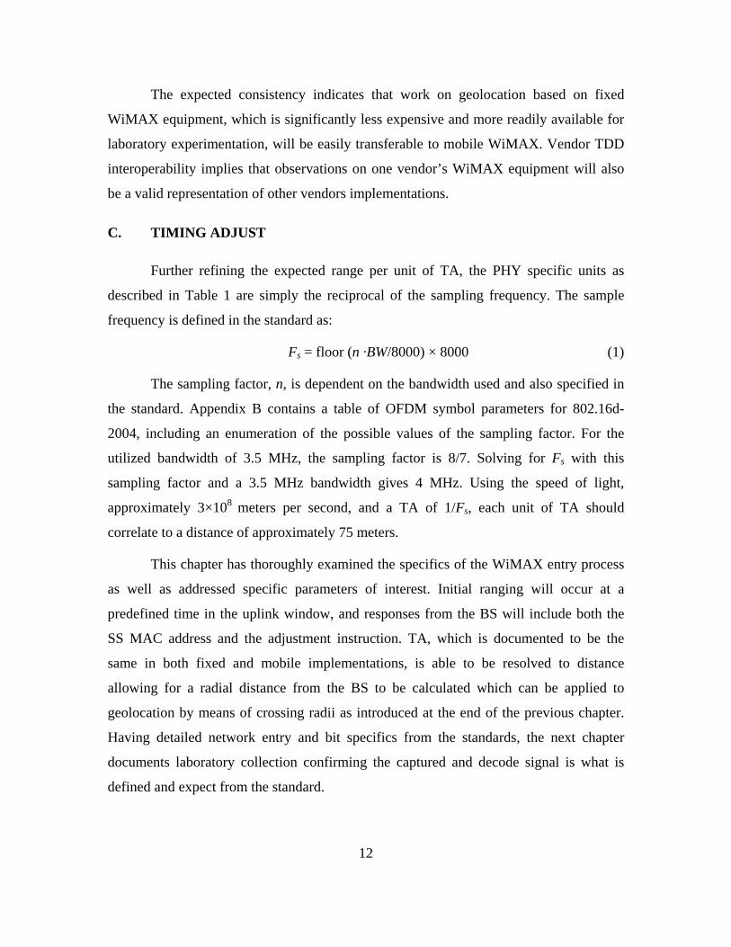
Further refining the expected range per unit of TA, the PHY specific units as

described in Table 1 are simply the reciprocal of the sampling frequency. The sample

frequency is defined in the standard as:

Fs = floor (n ·BW/8000) × 8000 (1)

The sampling factor, n, is dependent on the bandwidth used and also specified in

the standard. Appendix B contains a table of OFDM symbol parameters for 802.16d-

2004, including an enumeration of the possible values of the sampling factor. For the

utilized bandwidth of 3.5 MHz, the sampling factor is 8/7. Solving for Fs with this

sampling factor and a 3.5 MHz bandwidth gives 4 MHz. Using the speed of light,

approximately 3×108 meters per second, and a TA of 1/Fs, each unit of TA should

correlate to a distance of approximately 75 meters.

This chapter has thoroughly examined the specifics of the WiMAX entry process

as well as addressed specific parameters of interest. Initial ranging will occur at a

predefined time in the uplink window, and responses from the BS will include both the

SS MAC address and the adjustment instruction. TA, which is documented to be the

same in both fixed and mobile implementations, is able to be resolved to distance

allowing for a radial distance from the BS to be calculated which can be applied to

geolocation by means of crossing radii as introduced at the end of the previous chapter.

Having detailed network entry and bit specifics from the standards, the next chapter

documents laboratory collection confirming the captured and decode signal is what is

defined and expect from the standard.

13

III. LABORATORY OBSERVATIONS

A. INITIAL OBSERVATIONS IN THE NPS NETWORKS LAB

To begin exploring the possibilities of geolocating a WiMAX SS based on TA

values, as had been explored with GSM’s timing advance [8],[9], traffic was first

analyzed to ensure RNG-RSP messages could be identified and the necessary information

was discernable as suggested by the standard. A small WiMAX network was configured

in the laboratory. The network consists of a Redline AN-100U BS and two Redline

RedMAX SU-O outdoor SS. The AN-100U was configured to use a center frequency of

3.40175 GHz with a 3.5 MHz bandwidth via network interface and in the laboratory

connected to a laptop hosting a file server application. The SS are simply connected to

120 V wall power without need for further configuration and, when attached to other

laptop terminals, sustained network traffic could be generated.

Collection of the air interface is achieved by an antenna situated between the BS

and SS, which feeds an Agilent 4440 Spectrum Analyzer and a Sanjole WaveJudge 4800

WiMAX analysis box. The WaveJudge is a passive protocol-analyzer which provides

protocol and higher-layer capture and decode capabilities and can correlate RF to MAC

data. Focusing on the MAC, the WaveJudge was the primary observation instrument,

able to capture and decode up to eight seconds of OFDM symbols and display the results

to a computer via universal serial bus (USB) data transfer. The limited capture time

shaped initial observation in limiting observations of the RNG-RSP to initial ranging, and

no periodic ranging was identified.

Viewing the decoded traffic, the RNG-RSP was observed for repeated trials at a

range of 10.5 meters, the length of the lab room. Table 2 shows a sample of the actual

bits in one of the RNG-RSP messages, illustrating the time length value format of the

packet, with information type and data length indicated before the data bits.

14

Management Message Type 5, Ranging Status 1 “Continue”

Type # Bytes Value

Timing Adjust 01 04 FF FF FF BE

Power Level Adjust 02 01 EB

Offset Frequency Adjust 03 04 00 00 00 7A

Table 2. Sample RNG-RSP Values.

Having successfully identified and verified the RNG-RSP contained a fairly

consistent TA at a static range, the SS were moved to assess the variability and resolution

of the TA at different ranges. Initial attempts to move both the BS and SS for maximum

range deltas were unsuccessful due to in-lab transmit power limitations and the

directional properties of the laboratory collection antenna precluding capture of traffic

with the BS relocated. Since only the downlink was of concern to capture RNG-RSP

messages, and RNG-REQ were less significant, the BS was left static in its original lab

location, and only the SS were moved. Later testing with greater ranges would provide

more amplifying data, but as other students were working on calibrated measurements,

disruption of the collection equipment was not yet feasible.

RNG-RSP observations varying the distance to the SS provided initially

promising results. Figure 6 shows the TA associated with range in meters. Of note,

repeated values at a given range cluster since the TA only takes on discrete values.

Overall, the results showed high correlation between range and TA, and the TA for

repeated trials at fixed range showed a standard deviation of 0.79, meaning most of the

time the TA was plus or minus one unit.

15

Figure 6. Laboratory RNG-RSP TA vs Distance.

Notably, at distances beyond 12 meters the SS were moved out of the laboratory

where the BS was located to a passageway. This configuration no longer provided line of

sight between the BS and SS and introduced more multipath in the RF link. Considering

this and the rather limited distances within the building, rather than simply using the data

trend line illustrated in Figure 6 to approximate change in TA with distance, the data

could also more broadly be interpreted to represent one cluster in the laboratory and one

cluster in the passageway. This still indicates very consistent results at similar distances,

with greater distances resulting in greater initial TA.

Finally, the observed TA were all negative, which recalling from the standards, is

defined to indicate the SS should be transmitting sooner. A larger negative number

indicates the SS should be making more and more correction to transmit earlier in time.

For the sake of clarity, all remaining discussion of TA during the initial ranging will

simply indicate the magnitude of the TA, so a great TA will reflect greater distance and

timing advance, avoiding any possible confusion with larger negatives being smaller.

16

B. OBSERVATIONS OF TEST DATA FROM SANJOLE

In the process of optimizing test methodology with the WaveJudge, during a site

visit and meeting with Sanjole Chief Technology Officer, Dr. Xavier Leleu, several other

capabilities of the WaveJudge were discussed beyond simply decoding the traffic from

the air interface. Sanjole had designed the WaveJudge to provide diagnostic capabilities

to equipment vendors after witnessing difficulties observing intersystem communications

at PlugFest events. In these settings, testing with the WaveJudge is often conducted over

wired channels, rather than the air interface as in the NPS laboratory.

Two interesting features that might be useful in automating geolocation were also

presented. The WaveJudge has scripting capability, which would allow specific parts of

the decoded WiMAX messages to be passed to another program over a TCP port.

However, use of this scripting feature requires additional licensing, and even using the

scripting feature, the WaveJudge still transfers the entire base band signal to the analysis

computer, creating a limited collection window based on available memory and

introducing extra delay during processing.

Another feature of WaveJudge is the ability to range certain packets. During a

bandwidth request, a WiMAX subscriber transmits one of 64 known PN codes. Just as

the BS can range the SS based on known codes during network entry, the WaveJudge can

find the range from its antenna’s location to the SS based on delay in the reception of the

PN code from the SS’s assigned transmission time seen in the uplink map.

Observing such ranges in Sanjole’s data from wired testing with the WaveJudge

logically collocated with the BS, the equivalent TA seen from the WaveJudge was

consistent with the BS’s TA in the RNG-RSP with the exception of a fixed offset. Leleu

reported that an offset between the transmit and receive channels has been observed in

most BSs, causing an offset value that the link is able to adjust for during the ranging

process by simply adjusting for it in the TA [13]. This agrees with and explains the offset

value seen in the initial collection in the NPS laboratory.

Ranging based on known PN codes from a collection and analysis box, such as

the WaveJudge, could easily add a second location from which to establish a radius to aid

17

in the geolocation process. However, while the initial RNG-RSP contains a MAC

address, responses to the PN code are simply addressed to whichever SS sent that specific

code of the 64 known codes, so more associated traffic would have to be stored and

correlated to specifically associate which SS was just ranged. This identification issue

will have to be addressed for periodic ranging cases as well, since after a connection

identifier is established, the network no longer references the MAC address. For the

duration of this paper, we will continue to focus specifically on ranging based on the

RNG-RSP.

This chapter began examining actual collection of the network entry process from

the air interface and illustrates a sample of actual time-length-value encoded bits decoded

from RF. This collection verified consistency with the standard, and collection within the

confines of the laboratory facilities began to show highly consistent values with linear

correlation to distance. Insights from the equipment vendor confirmed a timing offset can

exist between the BS send and receive channels, as well as highlighting the potential to

establish a range from the collection platform and the ability to use scripts to pipe timing-

data into other programs. With this ability to rapidly and automatically move the

decrypted TA to another program in mind, the following chapter explores the

development of a user interface as well as the underlying mathematics to calculate a

geolocation based on this timing data.

18


19

IV. INTERFACE DEVELOPMENT

A. GUI BACKGROUND

In order to facilitate the practical use of the method of crossing range radii from

two or more BSs or a BS and other collection sites capable of ranging based on known

PN codes, automated computation accessed through a graphic user interface (GUI) best

enables an emergency responder or tactical user without requiring in depth technical

background or complicated calculations. The use of any automated system requires user

understanding of its capabilities and limitations. While a GUI rapidly presents a location

approximation, it is important to remember that there is variation in TA measurements

and output locations represent a probable area and not certain point. The approximations

are also only based on the programs internal algorithm and the user may have other

information that further refines an accurate location approximation or refutes an errant

estimate. For instance, in a case where there are multiple intersections between two

radius rings, a computer will be unable to differentiate them, but other situational

information may cue a user to favor one intercept as having a higher likelihood of being

the SS’s actual location.

Such a GUI was developed in HTML with JavaScript, utilizing the Google Maps

API to provide access to global satellite and terrain maps. The web interface allows for

easy cross platform use without the need for custom hardware or map databases. The

general layout of the GUI consists of a simple form to accept BS and collector locations

with TA information before rendering the plot with site coordinates, range radius rings,

and a likely SS location ellipse. It would be possible to populate these fields from a

database containing known BS locations, a GPS position of the collector, and scripted TA

output feeds from an analysis device like the WaveJudge. For purposes of testing and

evaluation, the GUI also contains fields to input the known location of a SS so its true

location can be compared to the output approximation during trials. While the details of

the HTML implementation and syntax used with the Google Maps API are beyond the

scope of this paper, the complete code is included in Appendix C. The JavaScript section

20

of the code contains the mathematical implementation of the geolocation approximation

and the employed methodology is examined in detail below.

B. ENABLING APPROXIMATIONS

Utilizing a method of intersecting range radii based on propagation delay acquired

from signal internals, a number of initial working parameters were first established. As

discussed in Chapter II, assuming free space propagation at the speed of light,

approximately 3×108 meters per second, at the bandwidth used each unit of TA seen from

the BS increases the range radius by 75 meters. This provides the basis for all range radii

in the calculations, both limiting resolution to 75 meters in the best case scenario and

accepting that there are variance and deviation in measurement.

A further initial approximation is the use of a flat Earth to facilitate calculations

in Cartesian coordinates. While a flat Earth approximation does not introduce significant

error over typical cell ranges, which are only infinitesimally curved on the geode, it

simplifies calculations of range radii, intercepts, and probability polygons to work in a

meters-by-meters coordinate system. However, mapping the results back to the spherical

system of latitude and longitude on Earth’s surface requires a coordinate transformation.

Over the entire globe, parallels of latitude are all parallel with the equator and

effectively equally spaced. However, meridians of longitude converge at the poles. At the

equator, a degree of longitude is roughly equal to a degree of latitude. However, moving

toward the poles, the meridians converge so the distance per degree of longitude

diminishes while the distance per degree of latitude remains consistent. While this does

not affect the Cartesian calculation - ten meters by ten meters is the same no matter the

location - it does introduce some complication into mapping the results calculated on a

square grid back to the surface of the Earth.

As a simplifying assumption, it is approximated that over small distances the

convergence of meridians is negligible, so meridians of longitude are parallel. This is

analogous to the far field approximation generally employed in radio frequency analysis

that as the radius of curvature becomes exceedingly large at a distance from the

transmission source it can be modeled as a plane wave. Assuming both lines of latitude

21

and longitude to be self parallel, they form a rectangular grid. The results of Cartesian

calculations can simply be mapped from a square grid to a rectangular grid by

multiplication by a linear constant in each direction, drastically simplifying in

implementation without appreciable loss of fidelity.

A degree of latitude is approximately 110 kilometers, and the length of a degree

of longitude is calculated based on scaling this value at the equator by the cosine of the

latitude, resulting in equivalent distances at the equator and the length of a degree of

latitude collapsing to zero at the poles. While these approximations provide very accurate

results in most cases, very near the poles some anomalies may manifest in this coordinate

system mapping.

A final coordinate mapping concern is the orientation of the angles. In most two-

dimensional mathematical applications, the X axis is horizontal with the Y axis vertical.

Zero degrees is defined to be straight to the right in the positive X direction, while a

positive 90 degrees is counterclockwise a quarter revolution, straight up along the Y axis.

However, working on the globe, it is customary to define north as zero degrees, while 90

degrees is defined by turning clockwise to the east. This requires a 90-degree shift and

then an axis flip to overlay the coordinate systems. All of the trigonometric sine function

calculations still work on the flat Earth projection, but axis orientation must be taken into

account to maintain the proper reference frame.

C. LIKELY LOCATION CALCULATIONS

Given two stations, each with a known radius, the most likely location of an SS is

where the radius rings overlap or are closest to overlapping. Broadly, three basic

situations can occur: the radius circles can intersect, one radius circle can be completely

contained within the other, or the two radius circles can be separated without touching.

With only two stations, overlapping rings results in two intersections, one of which is the

coordinate solution to the most likely SS location based on those rings. A third station

will almost always remove the ambiguity, since all three rings only converge near one of

the two intersections of the two ring solution. Figure 7 illustrates the decision process as a

flow chart.

22

Figure 7. Flow Chart for Geolocation Method.

Initially limiting the number of range rings to two, based on available test

equipment, the best possible location estimate will occur as the two intersections get

closer and closer to the point where the radius circles only touch in one point. Given this

best fix is achieved with the radius circles barely touching, concentric or separated circles

also provide the possibility of an accurate approximation when they are close to touching.

Two radius circles that come very close but do not intersect is as valuable a solution as a

single intersection, but obviously the further apart the nonintersecting radii become the

less and less meaningful the result.

In order to determine which of the three basic cases has occurred, the algorithm

generalized in Figure 7 compares the distance between the sites, solved by the

Pythagorean Theorem based on their grid coordinates, to the sum and difference of their

radii. If the two radii combined do not sum to the total distance between sites, there is no

intersection, and the estimated location is simply the midpoint plus an approximation

radius based on a scaling factor and the distance between the station’s radius circles.

Alternately, if the distance between the sites is less than the difference in their

radii, one radius circle is completely contained within the other. As long as the sites are

23

not exactly collocated, in which case no direction information can be ascertained,

drawing a straight line through the sites on one side will result in the maximum

separation and on the other side the minimum separation where the radii circles are

closest together. Again, the approximation area is the midpoint where they are closest

together plus a radius scaled by a constant at the separation distance.

If the radius circles are neither self contained nor completely separate, then they

intersect. One approach to find their intersections would have been to iterate through all

the points used to draw the radius circles on the map and find the ones that are closest

together based on a tolerance for rounding and the limited number of points used to

approximate a circle. More accurately and directly though, the method used to find the

intersections is based on triangles. The geometry of this method is illustrated in Figure 8.

The distance to the middle of the circles overlapping can be easily determined

from the law of cosines based on the site radii and total distance. To derive this, the

Pythagorean Theorem is simply applied to both of the triangles, knowing each

hypotenuse is the radius and the base is the total distance between sites less the distance

from the midpoint to the other site. Since both triangles share the last side, solving each

triangle for this side, the two equations can be set equal and solved to find the distance

from either site to the midpoint.

Figure 8. Illustration of Geometry to Calculate Circle Intersections.

24

Both intercepts lie on a line perpendicular to the line between the sites through

this midpoint. Having calculated this base distance, and knowing the hypotenuse of the

triangle formed from a site, the midpoint, and an intersection is simply the radius of that

site, the triangle can be completely solved to find the distance from the midpoint to the

intercept that was eliminated in the previous derivation when the equations were set

equal. Having completely solved the triangle, the intersection location relative to either

the midpoint or the site can be calculated, needing only to take into account the

coordinate system constants so they plot at the appropriate latitude and longitude on the

map.

As an example, working in Cartesian coordinates with one BS at the origin and

the other a distance D along the X-axis, the X-coordinate of both intersections is

calculated from the radii, R, and inter-site distance, D:

2 2 21 2

2

R R DX

D

(2)

The Y-coordinates of the intersections would then be found via the Pythagorean Theorem to be:

22 2 22 1 2

1 2

R R DY R

D

(3)

While the likely probability ellipses for both contained circles and separate radii

are simply plotted as circles, in the intersection case an ellipse is drawn around the two

intersections. In a case where the correct intersection representing the SS can be

identified, the probability ellipse can be viewed as the area of overlap from variance-wide

TA bands. This variance value is refined in field testing, but for initial GUI

implementation with intersection ambiguity, the ellipse is plotted to contain both

intersections with the major axis is based on the distance between the intercepts and the

minor axis is based on the separation between range radii. The center of the ambiguous

two BS ellipse is the same midpoint calculated to solve the intercept positions and the

relative angle of the intercepts defines the tilt of the ellipse (this is simply 90 degrees

from the angle between the sites). Separate cases deal with whether the intersecting

25

circles centers both contained within the larger radius, overlapping from within, or

whether the two circles overlap from the outside to provide the most reasonable

approximation.

D. DISPLAYED RESULTS

After the calculations, the Web interface displays the map with both stations

displayed; their range radius rings, and the likely location ellipse polygon. Mousing over

the respective icons identifies the site and provides its range radius in meters. If a SS

coordinate was entered, it will also be displayed and have its distance to the center of the

approximation polygon in its mouse over popup. If no SS coordinates are entered, the SS

defaults to the ocean at equator and the prime meridian, effectively eliminating its display

in most cases at useful zoom levels. None of these icons display latitude and longitude

coordinates since it is already displayed at the top of the web page and would only clutter

the map.

Checking the details button provides an alert popup containing more information

about the processed calculations and causes the map to also display the ellipse center

point and the line connection the base sites. The API allows the Google Map to continue

to behave as a user would expect under these overlays so a user can pan and zoom the

map, switch between street maps, imagery, or terrain maps, and re-center the map by

clicking on the hand in the upper left.

While database lookups and scripted input may be future additions, even hand

entering observed values from the WaveJudge provides a baseline functional tool. The

sample import button simulates what might be able to be scripted to import by populating

fields with predefined values contained in the HTML for a test scenario in Monterey. The

user interface, after a run with this simulated import, is shown in Figure 9.

26

Figure 9. Sample GUI Screen Shot.

Having discussed the need for a GUI, this chapter addressed fundamental

mapping issues including scaling and coordinates transformations to present data on the

globe’s grid of latitude and longitude rather than simply in generic two-dimensional

Cartesian space. After discussing these basic issues, the details of the actual geolocation

calculation were discussed. There are three scenarios in which radii from two BS can be

used to find a location approximation dependent on the distance between the BS and the

radii established by their TA. In the case the radius circles intersect, the mathematics of

how to find the intersections of two radii was shown. These simple principles can be

extended to greater numbers of BS further refining geolocational accuracy, but first,

equipped with a GUI that can easily run on a laptop and facilitate near real time

geolocation from a collection vehicle, further field testing is conducted to measure the

distance seen per unit TA and variance in observed TA at fixed locations over real world

distances.

27

V. FIELD EXPERIMENTS AND RESULTS

Following basic lab testing to verify that the RNG-RSP packet could be captured

and having created a preliminary web-based program to estimate locations based on radii

from two known points, field testing was conducted. There were two main goals in field

testing. First, confirm that the TA captured in the RNG-RSP continued to linearly

correlate to distance between the BS and SS over several samples at more practical real-

world distances. Second, testing sought to establish variability in repeated measurements

at a fixed point. This variability in repeated measurements is crucial in determining the

accuracy of a location fix based on TA, since a high variance in TA at a fixed location

would lead to a rather large area of uncertainty in approximating a SS location.

A. TESTING LOCATION, CONFIGURATION, AND PROCEDURE

In order to conduct testing, the same Redline WiMAX equipment used in the lab

was used to establish a simple outdoor WiMAX network, consisting simply of the BS and

SS operating at 3.4175 GHz configured the same as in the laboratory. Since this WiMAX

frequency is in the licensed band, full scale testing could not be conducted on and around

the NPS campus in Monterey, so instead arrangements were made to conduct testing at

Camp Roberts, outside of San Miguel, CA.

The testing site around McMillan Airfield at Camp Roberts was predominately

flat terrain with some trees and small single-story buildings, providing primarily line of

sight conditions during testing. Conditions were clear, with temperatures approaching 35

degrees Celsius at midday. The only other signal in the vicinity of the WiMAX operating

frequency was an approximately 2-5 GHz spread spectrum signal creating negligible

interference.

Configuring the WiMAX network at Camp Roberts, the AN-100U BS and

antenna were mounted on top of a raised observation platform, with the antenna mounted

7 meters above the ground. The exact same cabling and settings were used as in the lab,

and the BS was powered up and left alone for the remainder of the testing. The SS was

28

attached to a portable wooden stand with the SS antenna at 2 meters above the ground.

Neither the BS nor SS were connected to other computers or data sources.

Network entry was facilitated simply by powering up the SS, which began the

network entry process, just as turning on a cell phone negotiates network entry even if the

user is not immediately placing a call. Powering down the SS and powering it back up at

the same location allowed for repeated captures of the network entry process to capture

multiple RNG-RSP messages at the same distance from the BS.

Collection in the field was done from a vehicle, simulating what would

realistically be done by emergency response personnel or tactical operators. Using a roof-

mounted omni-directional antenna, the WiMAX signal was captured from the air

interface by the WaveJudge. Manually clicking to open the RNG-RSP response packet in

the WaveJudge interface, the TA was extracted and recorded. GPS coordinates were also

manually entered from the output of a basic consumer Garmin nüvi 200. More advanced

scripting may still allow this data to be exported directly from the WaveJudge and a GPS

device to feed a geolocation program like the one developed in the previous chapter, but

manual data entry was still timely during the experimentation. Figure 10 diagrams the

configuration of test equipment. Photographs and a sample WaveJudge screen capture are

included in Appendix D.

Figure 10. Test Configuration.

29

Figure 11. Field Collection Station Locations.

The SS was set up at 6 different locations as shown in Figure 11, with trials run

until at least 5 TA were successfully collected. One exception occurred later in the day at

the final range of greater than 1 km when only one TA was successfully captured due to

equipment difficulties. Initial observations showed very high consistency between

repeated observations at fixed distances and what appeared to be predictably greater TA

with increasing distance.

B. NOTED CHALLENGES DURING FIELD TESTS

Several challenges presented themselves while working with the WaveJudge as a

piece of collection equipment. Sanjole designed the WaveJudge to provide vendor

laboratory analysis to aid with design and interoperability testing [13], not provide real

time output. As such, the entire collected OFDM waveform is shifted to baseband and

transferred to the analysis computer for decoding, rather than being broken out to the bit

stream and sent to the computer. Because of this design, there is a limited amount of time

the system can capture before it runs out of memory. During field collection it became

30

important to time trigger the WaveJudge to cycling power on the SS, otherwise the RNG-

RSP was not captured in the limited collection window. In execution, it was found with

the tested Redline SU-O SS, triggering collection at approximately 20 seconds after first

applying power to the SS fairly reliably captured the RNG-RSP in the eight-second

collection window. After a sample was collected off the air interface, the computer still

had to decode the base band signal, which introduced further delay into the process.

These issues do not discredit the numerical results or in any way devalue the

capabilities of the WaveJudge to capture RF and decode protocols, but we simply point

out that in this case the equipment is being used for something other than its initially

intended design purpose. To actually field an operational geolocation system, real time

processing to the bit stream, as is done by the SS modem, would allow triggering on the

RNG-RSP, allowing capture without having to fortuitously align the memory limited

collection window.

Another issue that arose in testing later in the day was thermal stress on the BS.

Initial collection in clear condition with minimal interference showed minimal errors in

any of the packets collected. Later in the day however, more and more errors occurred in

the captured streams, not only in the RNG-RSP, but the uplink maps, downlink maps, and

many other packets the WaveJudge simply decoded as error packets.

Initially, it was thought that the increasing range may have had an effect, although

WiMAX is specified to operate at much greater distances, but using higher gain antennas

did not have any effect, and even returning to a distance of less than half a kilometer did

not resolve the issue. However, by the end of the afternoon, temperatures at Camp

Roberts approached 36 degrees Celsius, and the BS is only specified to operate at up to

40 degrees [14], so operating the WiMAX network on the edge of specifications began to

induce errors. If a temperature-controlled space had been available for the BS unit, the

antenna did not seem to have any issues, and testing could have continued. However, due

to limitations of time and space, this concluded range testing.

31

Noting the effects of temperature on the BS, while our vehicle maintained

functioning temperatures for the collection suite, thermal stress is definitely something to

take into consideration in designing systems for fielded operational use.

C. FIELD TEST RESULTS

Despite the noted issues that arose during collection, the experimentation was

successful, and after combing the results of the tests at various ranges, a continued trend

of tightly grouped TA with linear progression corresponding to distance from the BS was

observed. The collected data is plotted in Figure 12 with results summarized in Table 3.

Taking into account a basis offset from the delay between the BS transmit and receive

channels and cabling between the BS and BS antenna based on the measurements in the

lab, the results show an average meters per unit of TA is 36.99 with a standard deviation

of 3.10.

Figure 12. Field Test RNG-RSP TA vs Distance.

32

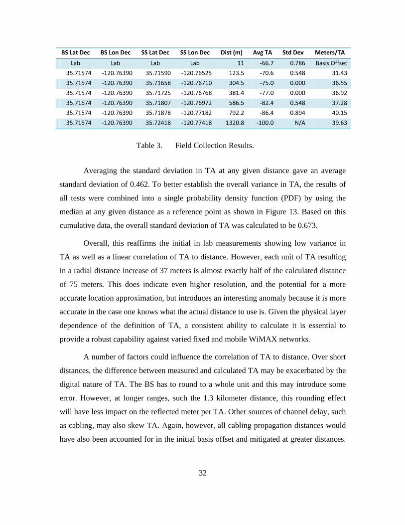
BS Lat Dec BS Lon Dec SS Lat Dec SS Lon Dec Dist (m) Avg TA Std Dev Meters/TA

Lab Lab Lab Lab 11 ‐66.7 0.786 Basis Offset

35.71574 ‐120.76390 35.71590 ‐120.76525 123.5 ‐70.6 0.548 31.43

35.71574 ‐120.76390 35.71658 ‐120.76710 304.5 ‐75.0 0.000 36.55

35.71574 ‐120.76390 35.71725 ‐120.76768 381.4 ‐77.0 0.000 36.92

35.71574 ‐120.76390 35.71807 ‐120.76972 586.5 ‐82.4 0.548 37.28

35.71574 ‐120.76390 35.71878 ‐120.77182 792.2 ‐86.4 0.894 40.15

35.71574 ‐120.76390 35.72418 ‐120.77418 1320.8 ‐100.0 N/A 39.63

Table 3. Field Collection Results.

Averaging the standard deviation in TA at any given distance gave an average

standard deviation of 0.462. To better establish the overall variance in TA, the results of

all tests were combined into a single probability density function (PDF) by using the

median at any given distance as a reference point as shown in Figure 13. Based on this

cumulative data, the overall standard deviation of TA was calculated to be 0.673.

Overall, this reaffirms the initial in lab measurements showing low variance in

TA as well as a linear correlation of TA to distance. However, each unit of TA resulting

in a radial distance increase of 37 meters is almost exactly half of the calculated distance

of 75 meters. This does indicate even higher resolution, and the potential for a more

accurate location approximation, but introduces an interesting anomaly because it is more

accurate in the case one knows what the actual distance to use is. Given the physical layer

dependence of the definition of TA, a consistent ability to calculate it is essential to

provide a robust capability against varied fixed and mobile WiMAX networks.

A number of factors could influence the correlation of TA to distance. Over short

distances, the difference between measured and calculated TA may be exacerbated by the

digital nature of TA. The BS has to round to a whole unit and this may introduce some

error. However, at longer ranges, such the 1.3 kilometer distance, this rounding effect

will have less impact on the reflected meter per TA. Other sources of channel delay, such

as cabling, may also skew TA. Again, however, all cabling propagation distances would

have also been accounted for in the initial basis offset and mitigated at greater distances.

33

Finally, there may be some degree of multipath adding additional propagation time

despite the clear, predominately line of sight conditions during testing.

Ultimately, since all of these TA modifying effects would be small and mitigated

over greater distances, the factor of two differences between the calculated and measured

TA is most likely a phenomenon unique to initial ranging. Recalling from Chapter II,

initial range occurs after the SS synchronizes to the received BS preamble. However,

since the BS does not know how long it took for its downlink to arrive at the SS, the first

delay it sees includes the time it took for the downlink to reach the SS plus the

propagation time for the SS’s initial ranging request to reach the BS. The total round-trip

time takes twice as long as the SS normal uplink to the BS, essentially decreasing the

meters per unit TA by two during initial range. However, despite the extra resolution this

provides during initial ranging, once the SS has an assigned uplink slot, continuing

periodic ranging adjustments may return to a range resolution of 75 meters.

Figure 13. Cummulative TA Probability Distribution from all Ranges.

34

This chapter discussed the details of field tests conducted to observe TA data over

distances more accurately simulating a cellular network environment. Having detailed

testing procedures and challenges, results from the field testing showed a very linear

progression of TA with increasing distance along with a very low variance in repeated

measurements at fixed SS locations, indicating the possibility for tightly bounded

geolocation probability ellipses. The range resolution during initial ranging turned out to

be twice as good as initial calculations from the parameters documented in the standard

had suggested, although this added resolution may be limited to the initial ranging

procedure. Having established a baseline for the performance of a standard compliant

WiMAX network in-field testing, the following chapter expands the hardware

constrained results through computer simulation to provide estimates of geolocation

accuracy in varied networks with multiple BS.

35

VI. MULTIPLE BASE STATION SIMULATIONS

While field and laboratory testing were limited to the one available BS, to better

understand the potential for geolocating a SS in a real world WiMAX network, several

multiple-BS scenarios were simulated in software. Using the data collected from the BS

in the field tests at Camp Roberts, MATLAB was used to simulate multiple BSs with the

same mean distance per unit of TA of 37 meter and standard deviation of 0.673 units TA.

While this assumes that all BSs in the network share the same characteristics as the one

AN-100U BS used in testing, it remains a reasonable premise based on the designed

interoperability within the standard.

A. TWO BASE STATION SIMULATION

First, two-BS scenarios were simulated using the algorithm developed in Chapter

IV to approximate the location of a SS based on two radii. The simulation created two

BSs at varying angles as observed by the SS, each with normally distributed random

distance with a mean of one kilometer from the SS, standard deviation in range of 300

meters, and TA fluctuations as observed through measurement. Since TA is a discrete

value, the BS first rounded distance to a whole unit of TA, and then on top of this an

error factor based on the observed variance seen in measurements was added. A Monte

Carlo simulation of one hundred thousand runs were conducted at each angle and the

average distance from the center of the approximation polygon (the midpoint between the

two circle intersections) to the actual SS location over these many runs was recorded.

At 180 degrees, the two BSs and SS form a straight line, and SS is location is

accurately approximated in the middle. However, as the angle collapses from this ideal

geometry, the two intersections of the radii get farther and farther apart, and since there is

ambiguity as to which intersection represents the location of the SS, the location

approximation of a midpoint between the intersections becomes farther and farther from

the true SS location. If other a priori knowledge could allow an operator to distinguish

between the two intersections, one of the intersections is always close to the SS, but the

algorithm alone cannot differentiate the two intersections. Interestingly, the estimate

36

distance collapses again once the angle between the BS approaches zero, since the BSs

and SS are again in a line. Figure 14 shows the overall results of this two BS simulation.

Figure 14. Distance to Midpoint Between Intersections with 2 BS Varying Angle.

B. MULTIPLE BASE STATION SIMULATIONS

Noting the limitations of a two-BS fix, a second set of simulations was conducted

in MATLAB using multiple BS. Except in rare cases introducing a third BS removes the

ambiguity between which of the intersections of the two BS represented the approximate

location of the SS. Figure 15 illustrates the sort of worst-case scenario that may occur

with a three-BS network which generates a very inaccurate location approximation by

essentially devolving to approximate a two-BS network.

The general approach of the multiple-BS simulation algorithms is simply to

calculate the intersections of each pair of BS radii, and then for each pair's intersections,

see which is closest to the nearest intersection of the next pair of BS’s radii. This

intersection should represent the intersection nearest the SS, and is added to an array of

intersections. Once this process has been repeated for all pairs, the array of closest

intersections forms the vertices for a small polygon approximating the location of the SS.

In the case of three BS, there are six intersections from the three pairs; producing three

37

chosen closest intersections, which when plotted should form a small triangle near the

actual SS location. In order to approximate the center of this polygon not knowing its

exact shape or number of vertices, the X component of each chosen intersection was

averaged to find the X coordinate for the center of the approximation, and the process

repeated with the Y coordinates from the same selected intersections.

Using this location-approximation algorithm with varying numbers of BS, several

BS-location scenarios were tested. First, all BS were placed at random angles from the SS

with normally distributed random distances with a mean of 1.2 kilometers and a standard

deviation of 400 meters. This completely random placement of BS was repeated for

100,000 runs at each number of BSs, and the average distance from the estimate to SS at

each number of BSs was recorded as in the earlier two-BS simulation.

As previously noted, an interesting result of the completely random BS placement

was that sometimes rare geometries would cause even the three-BS scenario to produce

an inaccurate result if the algorithm selected to weight a cluster of intersection where the

SS was not actually located. Basically, a three-BS fix can devolve to the two radii

ambiguity problem with unfortunate geometry as shown in Figure 15, where triangles

show towers, diamonds show selected intersections, the star shows the algorithm’s

estimated location and the square shows the actual SS location.

-1500 -1000 -500 0 500

-600

-400

-200

0

200

400

600

800

1000

1200

1400

3 Base Stations, 753 Meters from Estimate to Subscriber

Meters

Met

ers

Figure 15. Inaccurate Fix Situation with 3 BS.

38

Since all of the geometries are averaged in with the other runs, estimates that are

hundreds of meters off weigh in with many very accurate estimates from a three-BS

geolocation, as reflected in the results shown in Figure 16. Given that the overall average

error between the approximated center point and the SS is still only 80 m, there are many

more accurate fixes than the outlier cases (such as Figure 15) that pull up the average.

Appendix E contains more sample plots from the multiple-BS runs, including a

successful three-BS run that accurately estimates the SS location.

In a real world network, BS locations can be anticipated to be more logically

distributed. While actual tower locations in modern cellular networks rarely align exactly

to the idealized honeycomb cell layout, they are generally spaced to provide maximum

coverage with the least number of towers dependent on subscriber density. As such, two

follow-on multiple BS simulations were run that added some structure to the BS

placement. First, the angles were fixed to be evenly spaced based on the number of

towers while distances were randomly assigned as in the initial multiple-BS simulation,

and then for even further structure, the same even angle distribution was used but with all

BS at a one kilometer range from the SS. Figure 16 shows these results, which show

greater location accuracy than the completely random case. In networks with more

structured BS spacing the error estimate, despite TA rounding and variations, is still less

than 30 meters in all cases.

Figure 16. Average Distance from Estimate to SS with Multiple BS.

39

Based on these results, real-world scenarios can be expected to fall somewhere

between ideal and completely random geometries, so a geolocation fix assuming the

parameters measured in field testing can on average be expected to fall within 50 meters.

Appendix E contains sample plots generated during these different multiple-BS

simulations, and in many of these cases, the fix is well within 20 meters.

Having noted the discrepancy between the 37-meter average distance per unit TA

observed in initial ranging and the generalized calculated value of 75 meters per TA, the

simulations were re-run using 75 m as a basis instead. By increasing the distance between

differentiable radii, the resolution is reduced and the effect of rounding error is increased.

Figure 17 compares the results of the simulation using 37 and 75 meters per TA.

Interestingly, the geolocation accuracy of an ideal-geometry networks with 75 meter TA

units is nearly identical to that of a suboptimal geometry in a network with 37 m per unit

of TA.

As one would anticipate, the reduced resolution and greater rounding error leads

to somewhat larger approximation errors. None-the-less, expecting real-world BS

configurations to be between very structured and completely random, it is reasonable to

expect an average distance from the approximation center point to the subscriber to be

within 100 meters.

As an alternate presentation of this data, rather than using average distance from

the SS to estimated location over 100,000 trails, the same scenarios can be accessed via

circular error probable (CEP), that is the radius within which 50 percent of the samples

lie. The CEP for various numbers of BSs, with both BS geometry configurations and

distances per unit TA as before are shown in Figure 18. The same trends are seen as when

viewing the averages, but the circle containing 50 percent of the estimates has a smaller

radius than the average distance to the estimates calculated.

40

Figure 17. Comparision of Simulations with Different Distance per TA.

Using CEP, as before with averages, it is safe to assume that in more than 50

percent of cases, a SS can be geolocated within 50 meters assuming that accurate BS

locations are known.

Figure 18. Circular Error Probable from Multiple BS Simulations.

41

This chapter leveraged the collected real world data from field testing of a

WiMAX network and expanded it using computer simulation. Monte Carlo simulation

found that using average distance from approximation center point to SS location or CEP

as a metric, SS can consistently be located to within the distance per unit TA, less than 50

meters during initial ranging. Noting the TA anomaly in initial range, simulation results

showed excellent results for geolocation based on the standards explored in Chapter II,

the methods explored in Chapter IV, and the RF collection samples documented in

Chapters III and V.

42


43

VII. CONCLUSIONS AND RECOMMENDATIONS

A. CONCLUSIONS

Both laboratory and field testing indicate a high linear correlation to distance with

low variance in the TA observed in the initial ranging RNG-RSP message. Based on this

result, it is possible to establish a range radius from the BS. Using multiple range radii

from several BSs, or other devices capable of ranging the known WiMAX PN codes,

crossing radii can establish very accurate locations.

Results of simulation consistently showed that given the high resolution of TA

subdivisions within the signed 32-bit value and low variance at fixed distances,

geolocation should consistently be practical within a 50-meter CEP dependant on

accurate knowledge of TA offsets and values and BS tower locations. At the same time,

while high range resolution and low variance are extremely promising, the stipulations of

knowledge of TA anomalies and tower locations are non-trivial and important to consider

in fielding a geolocation system.

Having accurate BS locations to begin calculations is important, because any error

in tower location will be reflected in offsetting all intersections based on that BS.

Assuming BS locations to be known and cataloged in a database, it may be possible to

add a known initial TA offset from differences in transmit and receive channels, cabling,

and other site unique delays, but this too would necessitate site surveys, probably beyond

the level of detail typically conducted by a cellular network provider.

Also, while observed initial ranging showed TA radius rings with twice the

resolution calculated based on Equation 1 in Chapter II, the round trip delay phenomenon

may not appear when extrapolating these results to other periodic ranging occurrences

during continued network operation after initial entry. The fundamental methods and

principles to extract geolocation from TA data would remain the same, but using the

correct distance per unit TA is essential to correct geolocation.

44

With these practicalities in mind, the results of testing and simulation remain

extremely promising. The interoperability standards established by the WiMAX forum

provide that, taking due diligence, these results should easily extend to other vendor’s

equipment and the near verbatim replication of verbiage in the 802.16d-2004 and 802.16e

standards suggests easy adaption of this methodology to mobile WiMAX taking into

account adjustments to physical layer dependent parameters. Furthermore, WiMAX’s

chief competitor for 4G cellular, Long Term Evolution (LTE), also operates in a very

similar manner, featuring FDD and TDD profiles, of which the TDD internals could

similarly be used to geolocate just as explored here for WiMAX networks.

Using the principles explored through testing and simulation, it is possible to

geolocate a WiMAX SS within approximately 50 meters, offering potentially 10 times

better location accuracy than the GSM methods previously explored in literature, and

providing a great capability to be further developed and explored for use both by

emergency response personnel and tactical users.

B. RECOMMENDATIONS

Future research should confirm the application of these findings to mobile

WiMAX networks and further investigating periodic ranging and other opportunities to

extract geolocation data from WiMAX signal internals. Collection and fixes based on

actual multi-BS networks, rather than simulation alone, should be conducted to verify and

solidify the results in this thesis. Actual collection in real-world multi-tower networks

will also motivate the issue of identifying and caching unique identifiers for different

towers and subscribers to properly associate traffic to its originator, which would be of

critical importance to a fieldable system. Related work may also apply these methods to

LTE wireless device, requiring an investigation of the LTE standards before applying the

techniques illustrated in this thesis applied to WiMAX.

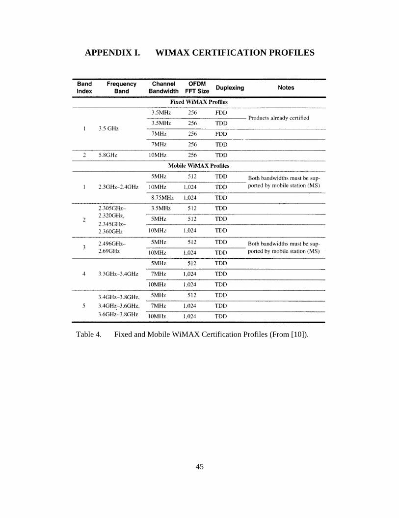
45

APPENDIX I. WIMAX CERTIFICATION PROFILES

Table 4. Fixed and Mobile WiMAX Certification Profiles (From [10]).

46


47

APPENDIX II. 802.16D-2004 OFDM SYMBOL PARAMETERS

Table 5. OFDM Symbol Parameters (From [12]).

48


49

APPENDIX III. GUI HTML/JAVASCRIPT CODE

<html>    <head> <title> OWL (v9.11b) </title> <script src="http://maps.google.com/maps?file=api&v=2&sensor=false&key=ABQIAAAAKg2XhyFKbQwX6KYN9UFtGBRzqH3tuoONQrJc0Yfxh_5EF-rAQBSuBt6V6Vzrd3cmnuVAjYdEHr3ImQ" type="text/javascript"></script> </head>  <body style="background-color:D3D3D3" onunload="GUnload()"> <noscript>Browser does not have JavaScript enabled!</noscript> <img src="images/npslogo.png" alt="NPS Logo" align="left"> <img src="images/nightowl.png" alt="Hedwig" align="right"> <h1 style="text-align:center"><i>O</i>FDM <i>W</i>ireless <i>L</i>ocator </h1> <p align="center"> <i>Version 9.11b</i><br/> TA is set for <i>BW</i>= 3.5 MHz. Please enter latitude/longitude in decimal degrees (<a href="http://www.fcc.gov/mb/audio/bickel/DDDMMSS-decimal.html/" target="_blank">converter</a>).</p>  <form name="inputForm"> <table align="center" summary="Data entry fields."> <tr> <td><b>SITE 1 (Base Station)</b></td> <td>Lat:</td><td> <input type="text" name="S1LAT"/></td> <td>Lng:</td><td> <input type="text" name="S1LNG"/></td> <td></td> <td>Offset:</td><td> <input type="text" maxlength="10" name="S1OFF"/> </td> <td>TA:</td><td> <input type="text" maxlength="10" name="S1TA"/></td> </tr><tr> <td><b>SITE 2 (Collector)</b></td> <td>Lat:</td><td> <input type="text" name="S2LAT"/></td> <td>Lng:</td><td> <input type="text" name="S2LNG"/></td> <td></td> <td></td> <td></td> <td>TA:</td><td><input type="text" maxlength="10" name="S2TA"/></td>

50

</tr><tr> <td><b>MARK (Subscriber)</b></td> <td>Lat:</td><td> <input type="text" name="MLAT"/></td> <td>Lng:</td><td> <input type="text" name="MLNG"/></td> <td></td> <td></td>  <td><input type="button" value="Import" onClick=" S1LAT.value='36.5986'; S1LNG.value='-121.8769'; S1OFF.value='67'; S2LAT.value='36.5909'; S2LNG.value='-121.8624'; S1TA.value='82'; S2TA.value='7'; MLAT.value='36.5949'; MLNG.value='-121.8651'; "> </td>    <td> </td>  <td><input type="button" value=" Plot " onClick="doit()"> Details:<input type=checkbox name="alertCheck"> </td> </tr></table> </form>  <script type="text/javascript"> <!-- function doit() { /********************** * Parameters & Values * **********************/ // Start Time var startTime = new Date(); // Constants pi = Math.PI; // Set Value of Pi c = 299792458; // Speed of Propagation (m/s) Fs = 4000000; // Sampling Frequency (PHY Dependent) mTA = c / Fs; // Meter per unit TA mLat = 111131.75; // Meters per Degree Latitude (Approx Const) // Meters Per Degree Longitude Based on Site Latitude latRad = inputForm.S1LAT.value*pi/180; mLng = (111412.84*Math.cos(latRad))-(93.5*Math.cos(3*latRad))+ (0.118*Math.cos(5*latRad));

51

// Number of Points to Use in Circle Approximation npts = 40; // Distribution Weighting for Probability Ellipse eProbDist = 1.2; // Site Locations from Form s1lat = inputForm.S1LAT.value; s1lng = inputForm.S1LNG.value; s2lat = inputForm.S2LAT.value; s2lng = inputForm.S2LNG.value; /**************************** * Range Radius Calculations * ****************************/ // Calculate Circles Radii // Site 1 s1ta = inputForm.S1TA.value - inputForm.S1OFF.value; s1r = s1ta * mTA; // Site 1 Range Radius in meters s1rLat = s1r / mLat; // Latitude Variance from Radius s1rLng = s1r / mLng; // Longitude Variance from Radius //Site 2 s2r = inputForm.S2TA.value * mTA; s2rLat = s2r / mLat; // Lat/Lng Delta from Radius s2rLng = s2r / mLng; // Invalid Timing Adjust Input Warning if(s1ta<0||inputForm.S2TA.value<0){ alert("Input Error: Net Negative Timing Adjust");} // Create Circle Arrays var s1cLat=new Array(); var s1cLng=new Array(); var s2cLat=new Array(); var s2cLng=new Array(); // Create Arrays to Hold Gmap Lat/Lng var s1Glatlng=new Array(); var s2Glatlng=new Array(); // Loop to Populate Radii Lat/Lng Arrays for(var i=0; i<= npts; i++) { angle=i*2*pi/npts; //Angle in Radians cosangle = Math.cos(angle); //Math Function for Cosines sinangle = Math.sin(angle); // Calculate Circles in Rectangular Coordinates /* x1 Forces Addition vice String Concatenation */ s1cLat[i]=s1lat *1 + (s1rLat * cosangle); s1cLng[i]=s1lng *1 + (s1rLng * sinangle); s2cLat[i]=s2lat *1 + (s2rLat * cosangle); s2cLng[i]=s2lng *1 + (s2rLng * sinangle);

52

// Create Gmaps Coordinate Arrays s1Glatlng[i]=new GLatLng(s1cLat[i],s1cLng[i]); s2Glatlng[i]=new GLatLng(s2cLat[i],s2cLng[i]); } /***************************************** * High Probability Polygon Approximation * *****************************************/ // Inter Site Distance via Pythag deltaLat=(s2lat-s1lat)*mLat; deltaLng=(s2lng-s1lng)*mLng; dist=Math.sqrt(deltaLat*deltaLat+deltaLng*deltaLng); // Angle Set to 0 = North phi=Math.atan2(deltaLng,deltaLat); cosphi=Math.cos(phi); sinphi=Math.sin(phi); bearS1toS2=Math.round(phi*180/pi); //Displayed Output Only if (bearS1toS2<0){ bearS1toS2=bearS1toS2+360;} // Calculate Intersection if(dist>s1r+s2r){ methodAlert="Seperated Radii"; deltaR=dist-s1r-s2r; mpLat=s1lat*1+cosphi*(s1r+0.5*deltaR)/mLat; mpLng=s1lng*1+sinphi*(s1r+0.5*deltaR)/mLng; major=deltaR*eProbDist; minor=major; psi=0; } else if(dist<Math.abs(s1r-s2r)){ methodAlert="Contained Circles"; if(s1r>s2r){ deltaR=s1r-s2r-dist; mpLat=s1lat*1+cosphi*(s1r-0.5*deltaR)/mLat; mpLng=s1lng*1+sinphi*(s1r-0.5*deltaR)/mLng; } else{ deltaR=s2r-s1r-dist; mpLat=s1lat*1+cosphi*(-s1r-0.5*deltaR)/mLat; mpLng=s1lng*1+sinphi*(-s1r-0.5*deltaR)/mLng; } major=deltaR*eProbDist; minor=major; psi=0; } else{ methodAlert="Intercepts"; // Distance from Site 1 to Midpoint s1mp=(s1r*s1r-s2r*s2r+dist*dist)/(2*dist); // Distance from Midpoint to Intersection

53

mp2i=Math.sqrt(s1r*s1r-s1mp*s1mp); // Midpoint Coordinates mpLat=s1lat*1+s1mp*(s2lat-s1lat)/dist; mpLng=s1lng*1+s1mp*(s2lng-s1lng)/dist; // Intersection Coordinates /* Note Final Coordinate Transform Constants */ int1Lat=mpLat*1+mp2i*(s2lng-s1lng)/dist*(mLng/mLat); int1Lng=mpLng*1-mp2i*(s2lat-s1lat)/dist*(mLat/mLng); int2Lat=mpLat*1-mp2i*(s2lng-s1lng)/dist*(mLng/mLat); int2Lng=mpLng*1+mp2i*(s2lat-s1lat)/dist*(mLat/mLng); // Angle Between Intercepts is Pi/2 from Intersite Angle psi=phi+(pi/2); // Define Ellipse Axis Lengths // Adjust Midpoint if Both Foci within One Radius if (dist>s1r&&dist>s2r){ minor=(s1r+s2r-dist)*eProbDist; } else if (s2r<s1r){ minor=(dist+s2r-s1r)*eProbDist; mpLat=s1lat*1+cosphi*s1r/mLat; mpLng=s1lng*1+sinphi*s1r/mLng; } else { minor=(dist+s1r-s2r)*eProbDist; mpLat=s2lat*1-cosphi*s2r/mLat; mpLng=s2lng*1-sinphi*s2r/mLng; } major=(minor+mp2i)*eProbDist; } // Calculate Probability Ellipse Bounds // Create Ellipse Arrays var peLat=new Array(); var peLng=new Array(); var peGlatlng=new Array(); cospsi=Math.cos(psi); // Angle Parameters of Ellipse sinpsi=Math.sin(psi); // Constant So Outside Loop halfnpts=npts/2; // Use 1/2 Number Points in Circle for Ellipse for(k=0; k<=halfnpts; k++){ beta=k*4*pi/npts; //Parametric Angle in Radians cosbeta=Math.cos(beta); sinbeta=Math.sin(beta); // Ellipse Defined in Rectangular Coordinates peLat[k]=mpLat*1 + (major*cosbeta*cospsi -

54

minor*sinbeta*sinpsi)/mLat; peLng[k]=mpLng*1+ (major*cosbeta*sinpsi + minor*sinbeta*cospsi)/mLng; // Create Gmaps Coordinate Array peGlatlng[k]=new GLatLng(peLat[k],peLng[k]); } // Distance from Ellipse Center to Marker via Pythag cmLat=(mpLat-inputForm.MLAT.value)*mLat; cmLng=(mpLng-inputForm.MLNG.value)*mLng; cmdist=Math.sqrt(cmLat*cmLat+cmLng*cmLng); /********************* * Output and Display * *********************/ // Map Initialization Function if (GBrowserIsCompatible()) { var map = new GMap2(document.getElementById("map_canvas")); map.setMapType(G_PHYSICAL_MAP); map.setCenter(new GLatLng(inputForm.S1LAT.value, inputForm.S1LNG.value), 14); map.setUIToDefault(); // Site Radius Circles var s1circle = new GPolyline(s1Glatlng,"#ff00ff",5); map.addOverlay(s1circle); var s2circle = new GPolyline(s2Glatlng,"#0000ff",5); map.addOverlay(s2circle); // Probability Ellipse var probell = new GPolygon(peGlatlng,"#f33f00",5,1,"ff0000",0.33); map.addOverlay(probell); // Marker for Subscriber Location if Known /* Null Input Defaults to Equator at Prime Meridan */ var mark = new GLatLng(inputForm.MLAT.value, inputForm.MLNG.value); var iconSS = new GIcon(); iconSS.image = "images/redSS.png"; iconSS.shadow = "images/shadow.png"; iconSS.iconSize = new GSize(32, 37); iconSS.shadowSize = new GSize(51, 37); iconSS.iconAnchor = new GPoint(16, 37); SStitle = "Subscriber Station \rDist to CP: " + Math.round(cmdist) + " m"; map.addOverlay(new GMarker(mark,{icon:iconSS, title:SStitle})); // Rounded Site Radii for Display s1rR=Math.round(s1r); s2rR=Math.round(s2r);

55

// Markers for Site Locations var site1 = new GLatLng(s1lat,s1lng); var iconBSpink = new GIcon(); iconBSpink.image = "images/pinkBS.png"; iconBSpink.shadow = "images/BSshadow.png"; iconBSpink.iconSize = new GSize(22, 32); iconBSpink.shadowSize = new GSize(39, 32); iconBSpink.iconAnchor = new GPoint(11, 16); BS1title = "Base Station (S1) \rRadius: " + s1rR + " m\rS2 Bearing: " + bearS1toS2; map.addOverlay(new GMarker(site1,{icon:iconBSpink, title:BS1title})); var site2 = new GLatLng(s2lat,s2lng); var iconBSblue = new GIcon(); iconBSblue.image = "images/blueBS.png"; iconBSblue.shadow = "images/BSshadow.png"; iconBSblue.iconSize = new GSize(22, 32); iconBSblue.shadowSize = new GSize(39, 32); iconBSblue.iconAnchor = new GPoint(11,16); BS2title = "Site 2\rRadius: " + s2rR + " m"; map.addOverlay(new GMarker(site2,{icon:iconBSblue, title:BS2title})); // Detail Alert Message if (inputForm.alertCheck.checked){ // Straight Line Between Sites var centerLine = new GPolyline([ new GLatLng(s1lat,s1lng), new GLatLng(s2lat,s2lng) ],"#ffff00",5); map.addOverlay(centerLine); mpLatR=Math.round(mpLat*10000)/10000; mpLngR=Math.round(mpLng*10000)/10000; // Mark Center Point of Approximation Ellipse var MPmark = new GLatLng(mpLat,mpLng); CPtitle = "Ellipse Center Point\rLat: " + mpLatR + "\rLng: " + mpLngR; map.addOverlay(new GMarker(MPmark,{title:CPtitle})); var endTime = new Date(); alert( "Time to Execute Script: " + (endTime.getTime() - startTime.getTime()) + " ms " + "\rPoints Utilized in Radius Circles: " + npts + " " + "\rCorrected Site 1 TA: " + s1ta + " 1/Fs " + "\rMeters per Degree Longitude: " + Math.round(mLng) + " " + "\r\rDistance Between Sites: " + Math.round(dist) + " m " + "\rBearing from Site 1 to Site 2: " + bearS1toS2 + " " + "\rSite 1 Radius: " + s1rR + " m " +

56

"\rSite 2 Radius: " + s2rR + " m " + "\r\rMethod Used: " + methodAlert + " " + "\r\rEllipse Midpoint Lat: " + mpLatR + " " + "\rEllipse Midpoint Lng: " + mpLngR + " " + "\r\rDistance from Midpoint to Marker: " + Math.round(cmdist) + " m" ); } } } // --> </script>  <div id="map_canvas" style="center; height: 512px"></div> </body> </html>

57

APPENDIX IV. FIELD TEST IMAGES

Figure 19. Base Station.

Figure 20. Subscriber Station.

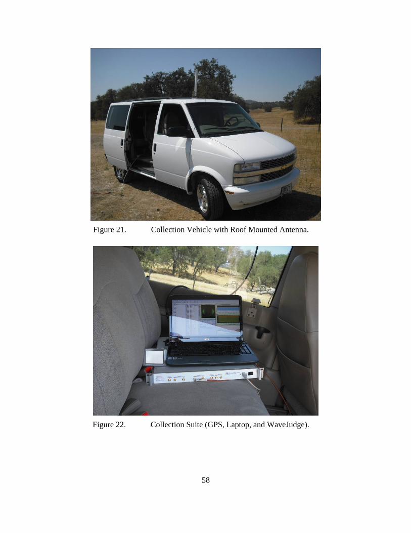
58

Figure 21. Collection Vehicle with Roof Mounted Antenna.

Figure 22. Collection Suite (GPS, Laptop, and WaveJudge).

59

Figure 23. Screen Shot of WaveJudge Interface with Captured RNG-RSP Open.

60


61

APPENDIX V. MULTIPLE BASE STATION SIMULATIONS

A. TWO BASE STATIONS THROUGH VARYING ANGLES

1. Two Base Stations Through Varying Angle MATLAB Code

% Two Base Station Simulation Varying Angle % LT D. E. Barber, NPS GSEAS % Rev. 12, 1 Sept 2009 clear all; % Measured Timing Adjust Parameters Based on Field Measurements mTA = 37; %Mean meters per Unit of Timing Adjust stdTA = 0.673; %Mean TA standard deviation % Synthetic Base Station Distance Parameters SiteMean = 1000; %Mean Site Distance SiteSD = 300; %Site Standard Deviation circlePts = 30; % Number of points in circle plots t = (0:circlePts)*2*pi/circlePts; % Initialize Arrays AngAvg = 0; errorDist = 0; for i = 0:18 %Iterate Angles in 10 Degree Steps theta = i*pi/18; %Angle from Subscriber to Base Station 2 for j = 1:100000 %Repeated Runs to Average % Distance to Simulated Base Stations with X/Y Coordinates DistBS1 = SiteSD*randn(1) + SiteMean; x1=DistBS1; y1=0; %BS on Axis DistBS2 = SiteSD*randn(1) + SiteMean; x2=cos(theta)*DistBS2; y2=sin(theta)*DistBS2; % Timing Adjust for Base Stations including Random Variation TABS1 = round(DistBS1/mTA) + round(stdTA*randn(1)); TABS2 = round(DistBS2/mTA) + round(stdTA*randn(1)); % Site Radii based on TA s1r = TABS1 * mTA; s2r = TABS2 * mTA; % Inter-Site Distance via Pythag and Angle from ATAN2 dist = sqrt((x2-x1)^2 + (y2-y1)^2); phi = atan2((y2-y1),(x2-x1)); % Find Midpoint Between Circles or Circle Intersections if(dist>s1r+s2r) % Separated Radii

62

deltaR=dist-s1r-s2r; mpX=x1+cos(phi)*(s1r+0.5*deltaR); mpY=y1+sin(phi)*(s1r+0.5*deltaR); elseif (dist<abs(s1r-s2r)) % Contained Circles if(s1r>s2r) deltaR=s1r-s2r-dist; mpX=x1+cos(phi)*(s1r-0.5*deltaR); mpY=y1+sin(phi)*(s1r-0.5*deltaR); else deltaR=s2r-s1r-dist; mpX=x1+cos(phi)*(-s1r-0.5*deltaR); mpY=y1+sin(phi)*(-s1r-0.5*deltaR); end else % Intersections s1mp=(s1r*s1r-s2r*s2r+dist*dist)/(2*dist); % Distance BS1 to Midpoint mpX=x1+s1mp*(x2-x1)/dist; mpY=y1+s1mp*(y2-y1)/dist; end % Distance from Midpoint to Subscriber at Origin errorDist(j) = sqrt(mpX^2+mpY^2); end AngAvg(i+1)=mean(errorDist); % Plot Once Every Other Angle if mod(i,2)==0 figure(i/2+1); clf; hold on; axis equal; title(['Base Station 1 on X Axis, Base Station 2 at ',... int2str(i*10), ' Degrees']); xlabel('Meters');ylabel('Meters'); plot(s1r*cos(t)+ x1, s1r*sin(t)+ y1,'-b'); plot(s2r*cos(t)+ x2, s2r*sin(t)+ y2,'-m'); plot(x1,y1,'^b','MarkerSize',10); plot(x2,y2,'^m','MarkerSize',10); plot(mpX,mpY,'rp','MarkerSize',10); plot(0,0,'sk','MarkerSize',10); hold off; end end

63

2. Two Base Stations through Varying Angles Example Plots

0 500 1000 1500 2000

-500

0

500

Base Station 1 on X Axis, Base Station 2 at 0 Degrees

Meters

Met

ers

-500 0 500 1000 1500

0

500

1000


Meters

Met

ers

-1000 -500 0 500 1000 1500-500

0

500

1000

1500

2000Base Station 1 on X Axis, Base Station 2 at 80 Degrees

Meters

Met

ers

-1000 0 1000 2000

-1000

-500

0

500

1000

1500


Meters

Met

ers

-1500 -1000 -500 0 500

-500

0

500

1000


Meters

Met

ers

-2000 -1000 0 1000 2000

-2000

-1000

0

1000

2000


Meters

Met

ers

Figure 24. Sample Plots from 2 BS Simulation with Varying Angles and Distances.

(Triangles denote the BSs, a square indicates the SS location , and the star shows

approximation center point.)

64

B. MULTIPLE BASE STATIONS

1. Multiple Base Stations MATLAB Code

% Multiple Base Station Simulation % LT D. E. Barber, NPS GSEAS % Rev. 14, 11 Nov 2009 clear all; % Simulation Parameters MaxNumberBS = 10; % Maximum Number of Base Stations to Simulate Runs = 100000; % Number of Runs at Each Number of Base Stations % Measured Timing Adjust Parameters Based on Field Measurements mTA = 37; % Mean meters per Unit of Timing Adjust stdTA = 0.673; % Mean TA standard deviation % Synthetic Base Station Distance Parameters SiteMean = 1200; % Mean Site Distance SiteSD = 400; % Site Standard Deviation circlePts = 180; % Number of points in circle plots t = (0:circlePts)*2*pi/circlePts; AvgError = 0:MaxNumberBS-2; % Average Error at N Base Stations StdError = 0:MaxNumberBS-2; % Standard Deviation at N Base Stations CEP = 0:MaxNumberBS-2; % CEP at N Base Stations % Number of Base Stations to Simulate for N = 2:MaxNumberBS % Initialize Sized Arrays DistBS = zeros(1,N); % Array to Hold Distance to Base Stations bsX = zeros(1,N); % Array of Base Station X Coordinates bsY = zeros(1,N); % Array of Base Station Y Coordinates bsTA = zeros(1,N); % Array of Timing Adjusts sr = zeros(1,N); % Array of Site Radius int1X = zeros(1,N); % Array for X Coordinate of First Intercept int1Y = zeros(1,N); % Array for Y Coordinate of First Intercept int2X = zeros(1,N); % Array for X Coordinate of Second Intercept int2Y = zeros(1,N); % Array for Y Coordinate of Second Intercept intX = zeros(1,N); % Array for Chosen Intercept from Pair's X Coord intY = zeros(1,N); % Array for Chosen Intercept from Pair's Y Coord DSE = zeros(1,Runs); % Array of Distances to Estimate Center Point for h = 1:Runs % Create Base Stations for i = 1:N % Number of Base Stations DistBS(i) = SiteSD*randn(1) + SiteMean; % Base Station Distance theta = 2*pi*rand(1); % Angle from Subscriber bsX(i) = cos(theta)*DistBS(i); % X Coordinate

65

bsY(i) = sin(theta)*DistBS(i); % Y Coordinate bsTA(i) = round(DistBS(i)/mTA) + round(stdTA*randn(1)); % Timing Adjust sr(i) = bsTA(i) * mTA; % Radius from Timing Adjust end % Find Two Intersections for Each Pair of Radii for a = 1:N b = mod(a,N)+1; % Inter-Site Distance via Pythag and Angle from ATAN2 dist = sqrt((bsX(b)-bsX(a))^2 + (bsY(b)-bsY(a))^2); phi = atan2((bsY(b)-bsY(a)),(bsX(b)-bsX(a))); % Find Midpoint Between Circles or Circle Intersections if(dist>sr(a)+sr(b)) % Separated Radii deltaR=dist-sr(a)-sr(b); % Closest Point Set as Both Intersections int1X(a)=bsX(a)+cos(phi)*(sr(a)+0.5*deltaR); int1Y(a)=bsY(a)+sin(phi)*(sr(a)+0.5*deltaR); int2X(a)=int1X(a); int2Y(a)=int1Y(a); elseif (dist<abs(sr(a)-sr(b)))% Contained Circles if(sr(a)>sr(b)) % Narrowest Set as Both Intersections deltaR=sr(a)-sr(b)-dist; int1X(a)=bsX(a)+cos(phi)*(sr(a)-0.5*deltaR); int1Y(a)=bsY(a)+sin(phi)*(sr(a)-0.5*deltaR); int2X(a)=int1X(a); int2Y(a)=int1Y(a); else deltaR=sr(b)-sr(a)-dist; int1X(a)=bsX(a)+cos(phi)*(-sr(a)-0.5*deltaR); int1Y(a)=bsY(a)+sin(phi)*(-sr(a)-0.5*deltaR); int2X(a)=int1X(a); int2Y(a)=int1Y(a); end else % Intersections s1mp=(sr(a)^2-sr(b)^2+dist^2)/(2*dist); % Dist from BS1 to Midpoint mp2i=sqrt(sr(a)^2-s1mp^2); % Dist Midpoint to Intercept mpX=bsX(a)+s1mp*(bsX(b)-bsX(a))/dist; % Midpoint X Coordinate mpY=bsY(a)+s1mp*(bsY(b)-bsY(a))/dist; % Midpoint Y Coordinate int1X(a)=mpX+mp2i*(bsY(b)-bsY(a))/dist; % First Intersection Coord int1Y(a)=mpY-mp2i*(bsX(b)-bsX(a))/dist; int2X(a)=mpX-mp2i*(bsY(b)-bsY(a))/dist; % Second Intersection Coord int2Y(a)=mpY+mp2i*(bsX(b)-bsX(a))/dist; end end % Select Closest Proximity Intersection from Each Pair for j = 1:N k = mod(j+1,N)+1; distFirst=sqrt((int1X(k)-int1X(j))^2+(int1Y(k)-int1Y(j))^2); dist12=sqrt((int2X(k)-int1X(j))^2+(int2Y(k)-int1Y(j))^2); if (dist12 < distFirst) distFirst = dist12; end distSecond=sqrt((int1X(k)-int2X(j))^2+(int1Y(k)-int2Y(j))^2);

66

dist22=sqrt((int2X(k)-int2X(j))^2+(int2Y(k)-int2Y(j))^2); if (dist22 < distSecond) distSecond = dist22; end if (distFirst < distSecond) % Store Selected Intersection in Array intX(j) = int1X(j); intY(j) = int1Y(j); else intX(j) = int2X(j); intY(j) = int2Y(j); end end % Approx Center of Polygon from Selected Intersections by Coord Mean EstimateX = mean(intX); EstimateY = mean(intY); %Distance from Subscriber to Estimate DSE(h) = sqrt(EstimateX^2+EstimateY^2); end AvgError(N-1) = mean(DSE); % Mean Estimate Error at N Stations StdError(N-1) = std(DSE); % Standard Deviation of Error CEP(N-1) = median(DSE); % Circular Error Prob at N Stations % Plot figure(N-1) clf; hold on; axis equal; title([int2str(N), ' Base Stations, ' int2str(DSE(h)), ... ' Meters from Estimate to Subscriber']); xlabel('Meters');ylabel('Meters'); for p = 1:N plot(bsX(p),bsY(p),'^b','MarkerSize',8); % Plot Base Station plot(sr(p)*cos(t)+ bsX(p), sr(p)*sin(t)+ bsY(p));% Plot TA Radius plot(int1X(p),int1Y(p),'ob','MarkerSize',4); % Plot Both Int plot(int2X(p),int2Y(p),'ob','MarkerSize',4); plot(intX(p),intY(p),'rd','MarkerSize',10); % Mark Selected Int end plot(0,0,'sk','MarkerSize',12); % Plot Subscriber plot(EstimateX,EstimateY,'rp','MarkerSize',12); % Plot Estimated hold off; end

67

2. Random Angle and Distance Example Plots

-3000 -2000 -1000 0

-2000

-1500

-1000

-500

0

500


Meters

Met

ers

-3000 -2000 -1000 0 1000 2000

-2000

-1000

0

1000

2000


Meters

Met

ers

-2000 -1000 0 1000 2000 3000

-2000

-1000

0

1000

2000


Meters

Met

ers

-1000 0 1000 2000 3000-3000

-2000

-1000

0


Meters

Met

ers

Figure 25. Sample Multilple BS Plots with Random Angles and Distances.

Triangles denote BSs, the square indicates the SS location, dots mark iterated

intersections, diamonds mark selected intersections, and a star shows approximation

center point.

68

3. Evenly Spaced Angles with Random Distance Example Plots

-2000 -1000 0 1000 2000

-2000

-1500

-1000

-500

0

500

1000


Meters

Met

ers

-2000 0 2000

-3000

-2000

-1000

0

1000


Meters

Met

ers

-4000 -2000 0 2000

-2000

0

2000

4000


Meters

Met

ers

-2000 -1000 0 1000 2000 3000

-3000

-2000

-1000

0

1000


Meters

Met

ers

Figure 26. Sample Multilple BS Plots with Equal Angles and Random Distances.



center point.

69

4. Evenly Spaced Angles with Fixed Radial Distance Example Plots

-2000 -1000 0 1000 2000

-1500

-1000

-500

0

500

1000

1500


Meters

Met

ers

-2000 -1000 0 1000 2000

-1500

-1000

-500

0

500

1000

1500


Meters

Met

ers

-2000 -1000 0 1000 2000

-1500

-1000

-500

0

500

1000

1500


Meters

Met

ers

-2000 -1000 0 1000 2000

-1500

-1000

-500

0

500

1000

1500


Meters

Met

ers

Figure 27. Sample Multilple BS Plots with Equal Angles and Fixed 1 km Distances.



center point.

70


71

LIST OF REFERENCES

[1] C. Eklund, R. B. Marks, K. L. Stanwood and S. Wang, "IEEE Standard 802.16: A Technical Overview of the WirelessMAN Air Interface for Broadband Wireless Access," IEEE Communications Magazine, pp. 98–107, June 2002.

[2] B. Bialek, "Analysis of 802.16 WiMAX networks," Naval Postgraduate School,

Monterey, California, December 2007. [3] WiMAX Forum, "Mobile WiMAX Plugfest," Bechtel Telecommunications,

Frederick, Maryland, September 2006. [4] Redline Communications. (2005, 11/9). Redline achieves TDD interoperability

with four WiMAX vendors at WiMAX Forum Plugfest in Beijing. [Online]. 2009(5/12), Available: http://www.redlinecommunications.com/news/pressreleases/2005/110905_02.html

[5] WiMAX Forum. (2009, November). WiMAX maps. [Online]. 2009(11/11),

Available: http://www.wimaxmaps.org/ [6] Federal Communications Commission, "FCC amended report to congress on the

deployment of E-911 Phase II services Tier III Service Providers," April 2005. [7] H. H. Loomis, "Geolocation of electromagnetic emitters," Naval Postgraduate

School, Monterey, California, November 1999. [8] M. A. Spirito and A. G. Mattioli, "Preliminary experimental results of a GSM

mobile phones positioning system based on timing advance," in Vehicular Technology Conference, 1999, pp. 2072–2076.

[9] G. P. Yost and S. Panchapakesan, "Improvement in estimation of time of arrival

(TOA) from timing advance (TA)," in IEEE 1998 International Conference on Universal Personal Communications, 1998, pp. 1367–1372.

[10] J. G. Andrews, A. Ghosh and R. Muhamed, Fundamentals of WiMAX:

Understanding Broadband Wireless Networking. Upper Saddle River, New Jersey: Prentice Hall, 2007, pp. 449.

[11] Institute of Electrical and Electronics Engineers, "IEEE Standard for Local and

Metropolitan Area Networks Part 16: Air Interface for Fixed and Mobile Broadband Wireless Access Systems," February 2006.

72

[12] Institute of Electrical and Electronics Engineers, "IEEE Standard for Local and Metropolitan Area Networks, Part 16: Air Interface for Fixed Broadband Wireless Access Systems," October 2004.

[13] X. Leleu, private communication, 1 July 2009. [14] Redline Communications. (2008, August). RedMAX base station (AN-100U)

system specifications. Redline Communications, Ontario, Canada. [Online]. 2009(7/24), Available: http://www.redlinecommunications.com/news/resourcecenter/productinfo/RedMAX_AN100u_ds.pdf

73

INITIAL DISTRIBUTION LIST

1. Defense Technical Information Center Ft. Belvoir, Virginia

2. Dudley Knox Library Naval Postgraduate School Monterey, California

3. Chair, Department of Electrical and Computer Engineering Naval Postgraduate School Monterey, California

4. Professor John McEachen

Naval Postgraduate School Monterey, California

5. Professor Herschel Loomis Naval Postgraduate School Monterey, California

6. Professor Vicente Garcia Naval Postgraduate School Monterey, California

7. Paul Greenfield National Reconnaissance Office/Advanced Systems & Technology Chantilly, Virginia

8. LTJG Tom Jones National Reconnaissance Office/Advanced Systems & Technology Chantilly, Virginia

NAVAL POSTGRADUATE SCHOOL - Defense … · NSN 7540-01-280-5500 Standard Form 298 (Rev. 2-89) ......

Documents

Transcript of NAVAL POSTGRADUATE SCHOOL - Defense … · NSN 7540-01-280-5500 Standard Form 298 (Rev. 2-89) ......