T git 'KW

TECHNICAL BTPOHT !

• UATK

^Wi-fiat.1. c.4^rc«a«*-o»

NPS55-78-008

NAVAL POSTGRADUATE SCHOOL

Monterey, California

SOME STATISTICAL PROCEDURES FOR THE

JOINT OIL ANALYSIS PROGRAM

by

D. R„ Barr

T „ Jayachandran

H, J. Larson

May 1978

Approved for public release; distribution unlimited.

Prepared for:~^AP-TSC NARF/Code 36nsacola, Fla. 32508

FEDDOCSD 208.14/2:NPS-55-78-008

NAVAL POSTGRADUATE SCHOOLMONTEREY, CALIFORNIA

Rear Admiral T. F. Dedman j. R . BorstingSuperintendent Provost

Reproduction of all or part of this report is authorized.

This report was prepared by:r /*) /O

UNCLASSIFIEDSECURITY CLASSIFICATION OF THIS PAGE (When Data Entered)

REPORT DOCUMENTATION PAGE READ INSTRUCTIONSBEFORE COMPLETING FORM

1. REPORT NUMBER

NPS55-78-0082. GOVT ACCESSION NO 3. RECIPIENT'S CATALOG NUMBER

4. TITLE (and Subtitle)

Some Statistical Procedures for the Joint OilAnalysis Program

5. TYPE OF REPORT ft PERIOD COVERED

Technical

6. PERFORMING ORG. REPORT NUMBER

7. AUTHORS.)

D. R. Barr, T. Jayachandran , H. J. Larson

8. CONTRACT OR GRANT NUMBERfs)

9. PERFORMING ORGANIZATION NAME AND ADDRESSNaval Postgraduate SchoolMonterey, Ca. 93940

10. PROGRAM ELEMENT, PROJECT, TASKAREA 4 WORK UNIT NUMBERS

P.O . # MME-77-006

It. CONTROLLING OFFICE NAME AND ADDRESSJOAP-TSC NARF/Code 360

Pensacola, Fla. 32508

12. REPORT DATEMarch 1978

13. NUMBER OF PAGES72

U. MONITORING AGENCY NAME 4 AODRESSf/ dltlerent from Controlling Office) 15. SECURITY CLASS, (of thta report)

Unclassified

1S«. DECLASSIFI CATION/ DOWN GRADINGSCHEDULE

16. DISTRIBUTION STATEMENT (of this Report)

Approved for public release; distribution unlimited.

17. DISTRIBUTION STATEMENT (of the abatract entered In Block 20, It different from Report)

16. SUPPLEMENTARY NOTES

19. KEY WORDS (Continue on reverse aide If neceeaary and Identify by block number)

Oil AnalysisStandard Artification

Laboratory CertificationElectrode Acceptance Tests

20. ABSTRACT (Continue on raverae aide It naceaaary and Identify by block number)

Procedures are described for1. Acceptance testing of prepared oil standards.2. Certification of spectrometric laboratories.3. Acceptance testing of graphite electrodes for use in the

oil analysis program.

dd ,;FORM ,,..,AN 73 "4/3 EDITION OF 1 NOV 65 IS OBSOLETE

S/N 0102-014- 6601 |

SECURITY CLASSIFICATION OF THIS PAGE (Whan Data Entered)

SOME STATISTICAL PROCEDURES FOR THE JOINT OIL ANALYSIS PROGRAM

FINAL REPORT FOR PROJECT ORDER MME-77-006

by

D. R. Barr

T . Jayachandran

H. J. Larson

Naval Postgraduate SchoolMonterey, CA 93940

May 19 78

TABLE OF CONTENTS

PAGE

I . INTRODUCTION 1

II . CALIBRATION STANDARDS 3

II . 1 . Introduction 3

II. 2. Characteristics of JOAP data 3

II . 3 . Tolerance Specifications . . . . 8

II. 4. The Test Procedure 22II . 5 . A Numerical Example 28II. 6. Summary of Calibration Standards

Testing 29

III . LABORATORY CERTIFICATION 3 4

III . 1 . Introduction 34III. 2. Spectrometer Certification 35III. 3. Interlaboratory Comparison 44III . 4 . Evaluation Testing 50

IV. GRAPHITE ELECTRODES 54

IV . 1 . Introduction 54IV. 2. Acceptance Criteria for

Graphite Electrodes 55IV. 3. Summary of Acceptance Criteria .... 64IV. 4. A Statistical Test to Evaluate

Trace Metal Content of GraphiteElectrodes as Determined on theA/E 35U-3 Spectrometer 66

IV. 5. Variance Contributed by Electrode... 68

SOME STATISTICAL PROCEDURES FOR THE JOINT OIL ANALYSIS PROGRAM

FINAL REPORT FOR PROJECT ORDER MME-77-006

by

D. R. Barr, H. J. Larson and T. Jayachandran

I. INTRODUCTION

The Joint Oil Analysis Program is a tri-service standardized

program to monitor equipment wear condition through the use of oil

analysis. Spectrometric oil analysis is used to determine the

type and amount of wear metals in lubricating fluid samples.

There are three primary factors that can affect the accuracy and

effectiveness of oil analysis.

1. The daily spectrometer calibration routine and

the particular oil standard used in the calibration.

2. The electrode type used in the analysis.

3. The experience and training of the spectrometer

operator/evaluator

.

This report describes statistical procedures developed under

a project sponsored by the Joint Oil Analysis Program Technical

Support Center, Pensacola, Florida and funded by the Engineering

Division, Kelly Air Force Base, San Antonio, Texas.

Statistical procedures for acceptance testing of new batches

of calibration standards are described in Section II. A three-part

statistical procedure for certification of the spectrometric

laboratories is presented in Section III. Section IV deals with

statistical acceptance tests of electrodes from different suppliers

In all three sections certain results of analyses of

experimental data supplied by the TSC are quoted. These data con-

sisted of acceptance testing readings of prepared oil standards

by three laboratories under ideal conditions. Since these ideal

conditions are not expected to occur in routine daily work, one

should be careful not to extrapolate these results to more general

situations. The numbers used in the worked examples came from the

same source and, again, may not be typical of what can be expected

in day-to-day laboratory work. The authors would like to

acknowledge the kind and generous assistance of Mr. Richard S. Lee,

Senior Army Representative of the Joint Oil Analysis Program

Technical Support Center, Pensacola, Florida. Any errors of

reasoning which may remain are the sole responsibility of the

authors

.

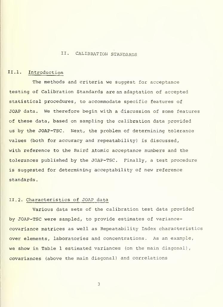
II. CALIBRATION STANDARDS

II. 1. Introduction

The methods and criteria we suggest for acceptance

testing of Calibration Standards are an adaptation of accepted

statistical procedures, to accommodate specific features of

JOAP data. We therefore begin with a discussion of some features

of these data, based on sampling the calibration data provided

us by the JOAP-TSC. Next, the problem of determining tolerance

values (both for accuracy and repeatability) is discussed,

with reference to the Baird Atomic acceptance numbers and the

tolerances published by the JOAP-TSC. Finally, a test procedure

is suggested for determining acceptability of new reference

standards

.

II. 2. Characteristics of JOAP data

Various data sets of the calibration test data provided

by JOAP-TSC were sampled, to provide estimates of variance-

covariance matrices as well as Repeatability Index characteristics

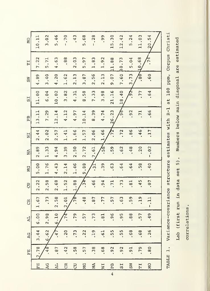
over elements, laboratories and concentrations. As an example,

we show in Table 1 estimated variances (on the main diagonal)

,

covariances (above the main diagonal) and correlations

cn

HrH

CNO

VO o COVO

COCM

CTi

asoCO

CNCN

COo

t* /in /

OrH

co IT) 1 m 1 inrH

CNrH

in rHrH

o /cn/

CNrH co

vo0000 o as

CO00

CNcr>

COCO

COo

COVO ft*>

p- LD *r CN in rH rH rHrH

orH

m o/

OS00

o oCN

CNvo

COrH 00

voin

COrH o

OVO

co/co

ovo

<* n t rH CN co CN CN OS r^ co/

oo o

CNO

CN00

rHCO

00in

coco

COOS

VOrH

o/as

r^r^

rHrH

VO orH

CO T CO r^ co rHCN

00 J

rHrH CN rH

CNrH Os rH

Osco

coCN /OS

CN rH vo

corH

r- CNrH

"^ 'd' orH

00 •^ VO /cn/

CNO

rH VOVO m

VOo

voVO /r»

CN VO00

vorH

<N CN CN rH rH rH CN iH/

as00

coco <7\

OSco

Oin

CN rHVO /m

(7\

inCNVO

CO oCN

CNO

CN rH *? co CN CN W 1

oo

VO m«vP rH

vo COCO /co

CTi

COcovo vo VO

00in

o

LD rH ^ CN rH °v

(N(N

00ID

00VO

CNin

0000 /co

VOVO OS

rH co rH00

mo

CN CN CN rH "y

VOco 00

inrHO /r*

CO00 m

COVO

asin

cr>

rHHrH

rH CN cn/ 1

oo

00CTi

orH /r-» in

CO rH00

VOCTi

inCTi

0000 in

o>

vo CN vo/

*&•^

CNVO /**

oCN

co CNCN rH

rHvo

inin

inm

00vo

COVO

VOCN

m v©/

00/*T 00

CN COin in

COCO

COVO

CNOS

CNCTi

rHas

as O00

ry

Wfa < 3

DU s 2

H PQ M MEh

oa

•H-Mcn T3•H (U

M +j

J5 rd

u 6•H

cn 4J

cn

Du QJ

>-i

CU

U 5-1

rd

*

£ rH

a rd

CU

o Cn

o rd

rH •H

-PfO c

•HrH

1

rd

e&

^s:-M rH

•H a)

5 X5

cn cn

<l)5-<

+J (U

R-§

•H 3-P SCO

0)•

<D^-.

M m3+J -P

U (U

3 cn

M-P rd

cn -Prd

(D XI

ofl crd •H

•Hi-i crd p> 5-1 (A

o Cf) •p

1cn •H

CI) u •P

o •H rd

c VH rH

m '—

'

<U

•H Hu A Hm rd

> ^ o

w

Eh

(below the main diagonal) for R-l at 100 ppm at the

Corpus Christi Lab. Typically, most of the correlations are

positive and many of the correlations are quite large. For

example, the estimated correlation between Pb and A£ analyses

is .96. This means that, within a single analysis, a Pb reading

above 100 was very likely to be accompanied by an A£ reading

also above 100; indeed, the relationship between Pb in a given

analysis and Ail in that same analysis was essentially linear

(with positive slope)

.

Such correlations substantially complicate the computational

difficulty of using a reference testing procedure that simultaneously

incorporates data from all elements. Therefore, we recommend a

procedure that continues the present practice of performing

separate analyses with each element. Even so, the correlation

among analyses for various elements (within a sample run) makes

precise evaluation of overall error rates of a testing procedure

difficult, a point we shall return to below.

In order to get an idea of the consistency of the repeat-

ability index over elements, labs and time, the variance in

analyses for individual sample runs was estimated for a number

of situations. For example, Table 2 shows estimates made from

data sets 1 and 5 in the data provided by the JOAP-TSC. From

these analyses, the following conclusions were reached:

UJ •«r CN rHCN rH CO ^« CN CN vo o in vo r*

o O ro vo r* CN cn cn CO "<r co T in vo mS

rH m TT VO *r T m

ro in rH roH CN ro cm cn ro o rH O CO r-

-H m CN O CN rH vo CO iH cn r- T in ro r~Eh

CN *» t ro o ro ro

m in rH F>00 VO vo o VO rH ro o r- CN o

C o ro rH cn o vo cn ro in m vo rH VO oCO

o CN *r ro rH ro ro

o rH rH r-ro o ^ CO *r o CN CN r* CN ro

-H o •<* CN CO CN CN t CO 00 CO VO ro ro COCO

ro in o ro -H CN ro

CO r* O invo V ^r o ^r "31 cn rH vo VO CN

ja o <s- ro r» o in ro CO in «a» *r vo in ro04

r» in r-» ro in ro «j«

ro rr o vo<*• r-i m rH rH r— en in CO vo ^r

•H CN n o tr rH ro CM r~ co vo 00 vo ro o55

CN rH cn ro o ro•

ro

vo o ro vo<N rr O CO CO CN rr ro rH vo cn

(0 CN ro m ro O rH CN CN •H m p* CN CN cnz

rH ^" cn in rH CN ro

r- vo CN rH<T> r- r- o O CO rH vo VO CN H

o> rH CN © ro rH o CO CD in t> in o CN CNa

CN in cn in rH ^r m

VO t vo 00CO CN r-t r» r*» o rH m vo vo r*

3 O co o o o rH r» ro r- cn «a« ^ iH mU •

o CN O CN CN CN CN

<Ti in in VO CNCO CO T)> VO CN o ro *r O CO CN

M CN rH ^r vo ro ro o rH in co r- in ro COO

CN ro CN CN rH CN CN

in in r* CNO vo -( vo ro vo rH "«• VO ro r»O ro CN T <» 'S' *r *» r- cn CO cn ^" VO

<CN ro rH TT O ro ro

CN CN r» r-'ST ro vo ro ro vo rr P* •«* r» CO

CP O CN ro cn ro o r~ r» co «<r *» CO rH lO<;

rH ro VO r» ro CN ^«

ro in ro r»r»> CO cn cn «r rH CO rH •*r o ^

0) o CN O ro o ro rH ro r* r- rH in ro infa

cnCN ro o ro O ro

M M M M t-t M )H M H M H Hxspui < « < « < « < cc < « < OS

Eaaro

sa,Q*oO

i

rH

avn u S On o 2 0*

T J.3S YJ.YQ s las viva<s> C»

H MOS «C CRJ (0

a <u

s E

rorH

rorH

r» r-

CNrH

ro

VO CO

rHrH

OrH

CO ^r

«q» cn

ro CNrH

rH rH

cn CN

orH

VO

CN rHrH

m m

m'OG

a)to

<dpca

QUou-i

Xa>

•oc

JQ(9u<a

&•oc(d

xvV

cM>1uid

u3O

i

CN

53

1

S Ea aa a,ro O

orH

a crd (0

rx OS

1) Variances among elements may differ significantly.

2) There is a weak but discernable pattern of variance

sizes among elements (for example, Cu is among the

lowest and Mo is among the highest)

.

3) There seems to be no consistent pattern of variance

sizes among labs.

4) Variance patterns among the two standards within a

sample run tend to be consistent. That is, high

variance in R-l Pb tends to go with high variance

in R-2 Pb for a given sample run.

5) High variance for one element in a sample run does

not imply other elements in that sample run are also

outside reasonable variance standards.

The above conclusions pertain to the particular data set on which

they are based and may not be typical of day-to-day routine

readings

.

Based on these conclusions, the following recommendations

are made concerning the test procedure:

1) Do the standards acceptability test separately for

each element (further supporting the present procedure

in this regard)

.

2) Since the reference standards are prepared by the TSC,

and a spectrometer is available to the TSC at Pensacola,

complete all reference standard acceptance testing

at the TSC„

II. 3. Tolerance Specifications

The data provided by the JOAP-TSC were used to investigate

how the repeatability index responded to changes in concentration

in a particular element, and to determine whether the response

characteristics were the same for all elements. This is important

since a statistical procedure will measure significance of

apparent differences in mean concentration in terms of underlying

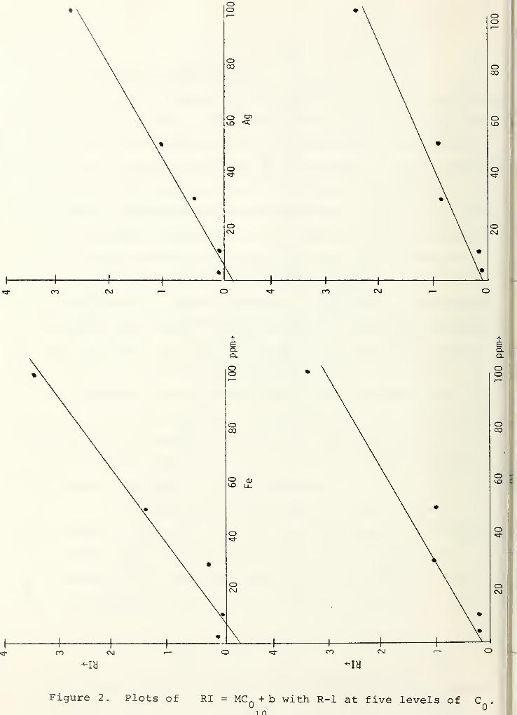
repeatability of analyses. It was found that, for most elements

with concentrations in the range 0-100 ppm, the repeatability

index increased as quadratic functions of initial concentrations

(see Figure 1) . However, adequate fit for practical purposes is

obtained with a linear function (that is, for practical purposes,

one may assume RI = mCn

+ b, where C- is the initial concen-

tration, m is the rate of increase in RI with Cn

and b is

the intercept) . As an example, Table 3 shows estimates of b

and m for both the linear fit and quadratic fit. These are

based on R-l analyses at the Pensacola Lab (last run) , at

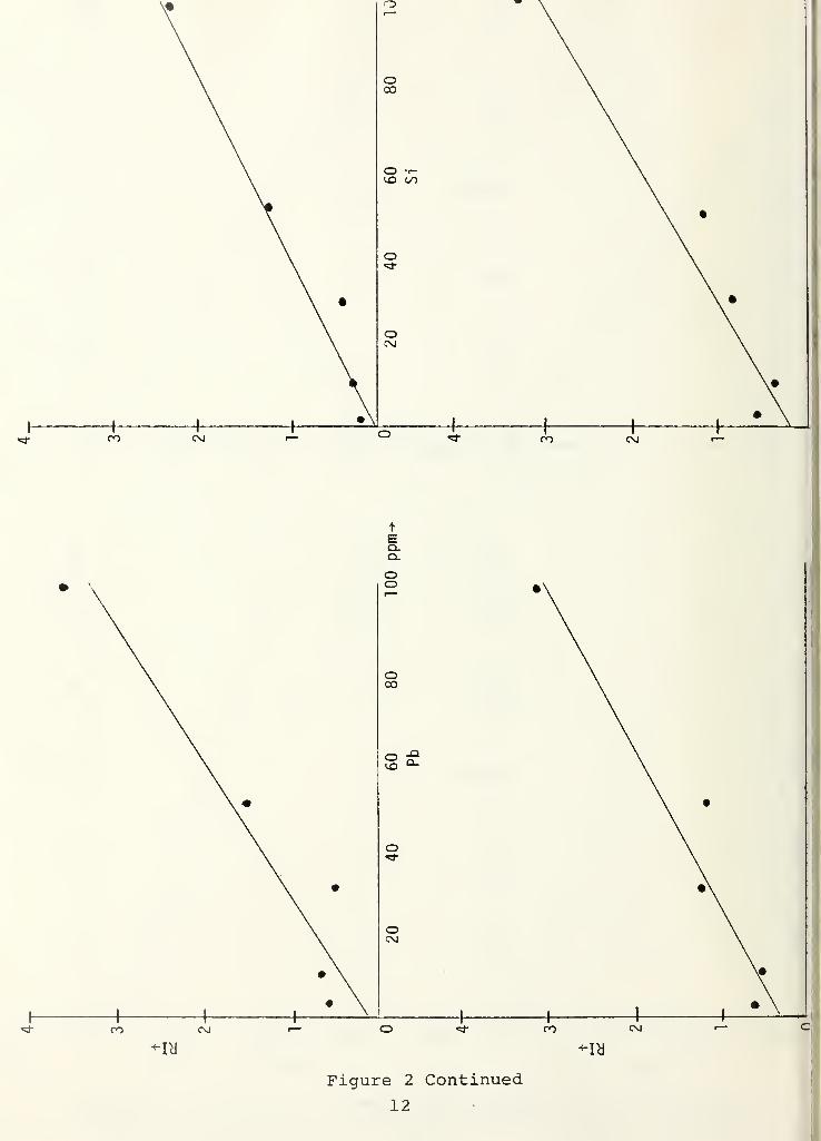
concentrations of 3, 10, 30, 50 and 100 ppm. Figure 2 shows

plots of the linear fit for 13 elements.

It was found the elements appear to have different

patterns of increase of RI with Cn

. This suggests a different

tolerance criterion should be used for RI for each element.

Adequacy of the linear and quadratic fits are indicated by the

estimated correlation values r in Table 3. Values of .95 or

oo

oCO

O C7,

O

o

oa

CO

O S-U3 C_)

o

oCM

c\j

a.a.

oo

CXI

a

OO

o

° ^

O

Ocxi

Figure 1. Plots of /RI = MC + b with R-l at five levels of C .

1 1 1

\%

1

\ •

\%

oo

oCO

o

O•3-

OCsJ

\

CD

1 1 1

\ •

1

\ •

1 1 11 1 1 1 1

oo

oCO

o

o*3-

oCM

ro CM CO CM

Figure 2. Plots of RI = MC n + b with R-l at five levels of C .

oo

CD

OCO

o

o

a

I

oo C\J

CLa

Q.Q.

OO

OCO

o ra

o

o

OO C\J

"lb

CO C\J

Figure 2 Continued11

o00

O •!-

o

oCM

-I hCO CM OO CM

Q.Q.

OO

O00

VO

o

oCM

HCO CM

^IcJ

CO CM

<-IcJ

Figure 2 Continued

12

-ia

Figure 2 Continued

J3

o•rl (1)^guno c a-P (0 o cr> r» (Tv ^ ID ^r<C U -H in "tj* CTt CM rH a\

co a. (N o CT» r^ O <Xi

"0 <H >i • • • • • •

n o +J

•H -U —(0

mo in o CM CTt

yo tr <T» en rH r-o o o en o O a\S

rH' '

rH'

n rH in in *r (T>

•H o T r^ <* rH l£>

Eh co O o r^- o a\* • • • • •

in rH o r^ CM CM

3 CM m KQ a\ t-i r->

(0 H o <T\ in o cr>

r» r^ CM ** rH oc o CM vo 00 rH e'-

CO co o CTt VD O en• • • • • '

00 co CM <T> CM co•H cm CM 00 r- rH COto o o en m O c\

1

" 'ft

• • '

^r ro r^ CM co u>£1 00 co in CO rH ina* o o o\ in o en

• • • • • •

in *r o\ en «# co•H o co 00 r^ rH cr>

s rH o er< in O CTi

• • 1 • • 8

co CO *y rH en kO<d o rH rH CO o ^J"

Z ^r O cr. «> o CO• • • * • •

CO o 00 , f> r» r»cr> in ^r CO r^ rH CO

£ rH o <Tt co o CTl

• t • • • •

1

o CO rH CM rH3 rH cm VD 00 rH inO o o CTt CO o CTt

*" • • • # • •

r« CM t*» r^ o oM rH CM r*> rH rH CTt

O rH O CTv in o en

r^ <T> CO U3 CM r^o? co CM in <T» rH r»< rH O a\ in O en

• • • • • •

m CM o 00 in r*>

D> r> CM o\ 10 rH en

< r-l O en CM o en

1

•

^r m co (N in ena) rH en CO rH rH CO

h rH o er» •<»• O er>

1

•

(0 o wa) •H (U

U +J P -Pm -P rd <fl -P fl

<U -H G, XX E U h-h e XI S UC <W -H tj m -h•H 4J nj -p

1-3 OT 3 CO

. w o r-i

39

14

more indicate satisfactory fit; values in excess of .98 indicate

quite close fit.

Values of RI computed for initial concentrations greater

than 100 ppm, which were diluted to 100 ppm for analysis, were

not significantly different from those for undiluted 100 ppm

initial concentrations. Note: It was found that several sample

runs for CQ

greater than 100 ppm had R-l data identical with

other sample runs. For example, data set 31 has the same R-l

data as data set 34 (and 30 has the same as 37) . Thus, it appears

the R-l concentrations for runs with initial concentrations

above 100 ppm (as shown on the computer print-outs) were in fact

accomplished with undiluted R-l standard at 100 ppm, in conjunction

with other standards testing. If this is the case, no difference

in RI due to dilution of more concentrated samples would exist,

of course, for R-l data.

Tolerances are needed for both accuracy and repeatability

of sample runs. Following accepted statistical principles,

the accuracy tolerances should depend on the inherent repeat-

ability of the analysis process. Thus, with analysis procedures

having high variance, one could detect only large differences

in the standards under test (if one desired to control, at

specified levels, the probabilities of committing errors in

one's conclusions). Theoretically, in order to test whether

two standards have the same concentration of a given element,

15

say iron, it is necessary to compare the difference in estimated

levels in each standard, measured in standard deviation units,

with a critical value taken from the statistical tables. For

purposes of illustration, we describe such a procedure in what

follows. If X, , X n , ... , X denote analyses of iron made withl z n

the old standard, and Y, , . . . , Y denote analyses of iron ininthe new standard (with analyses alternating between old and new,

as is current (and good) practice) , then

Tl =SX-Y

is compared with t~ ~ 1 ,~, wherer 2n-2;l-ct/2

X is the average of n consecutive analyses with

the old standard

Y is the average of n consecutive analyses with

the new standard

X) 2+ Z(Y.-Y)

2]

1/2

S = I- - is the estimated

Tz(X.-X) 2+ E(Y.-Y)^1 7

L - - ~ i!

X-Y L n(n-l) J

standard deviation of X-Y, and

t_ o . -i _ /j is the tabulated (l-a/2) 100th percentile

of the t-distribution with 2n-2 degrees of freedom,

16

A test would reject equivalence of the old and new standards

(and thus would reject the new standard for iron content) at

the a level of significance if |t| > t- that is,2n-2;l-a/2 '

if |X-Y| > S -t_^_Y 2n-2;l-a/2

The point of this illustration is not the test itself; rather,

it is to demonstrate how a "tolerance," in this case S-t, for

testing accuracy (X-Y) is a linear function of the joint

precision (repeatability), S. If different elements exhibit

varying characteristics of change in repeatability with changes

in initial concentration, then tolerance specifications should

likewise vary over elements and initial concentrations . It is

interesting to examine the accuracy and repeatability "acceptance"

tolerances listed in Tables 4-14 and 4-15 of T . . 33A6-7-24-1

(enclosure 2 of our data from TSC, hereafter referred to as

"Baird Atomic" acceptance tolerances) from this point of view.

It is easily verified that, within each group of elements,

AI is a linear function of RI_ . For example, for the group

{Ni, Si, Ai, Be Cr}, AI, = 1.885RIA

+ .233, with a correlation

very close to 1 . (It is also interesting to note that RI

in Table 4-15 of T.O. 33A6-7-24-1 is, within each element group,

nearly linear in initial concentration, consistent with our

finding that linear functions provide acceptable fits of the

apparent relationships between RI and CQ

.)

17

Comparison of the relationships estimated from

T.O. 33A6-7-24-1 with the theoretical coefficients from the

t-tables can provide some idea of the error rate levels one

might achieve using the Baird Atomic Acceptance tolerances.

Following the (2-sided, 2-sample t-test) argument above, theoretics

/2 tAI = 2n-2,l-g/2

RJ _

•n

For example, with n = 10 analyses from each standard and

a = .05 (the probability of rejecting the new standard iron

content, given it has in fact the same concentration of iron as

the old standard) , we would have

AI = H < 2 - 101 ' RI = .940 RT .

/ToA

From comparisons of Tables 4-14 and 4-15 of T.O .33A6-7-24-1, we

find approximately (for all groups of elements) AI z 1.9 (RI) + b

where b is a "calibration error allowance" of about .25 ppm.

In order to obtain the slope 1.9 in this relationship with the

t-test with n = 10, one would need to take a z .0005. Based

on this analysis, it appears that test procedures using the

tolerances given in Table 4-14 give quite conservative tests;

we suggest somewhat tighter tolerances with the procedure

recommended below.

18

There appear to be two major goals in the standards

testing activity. In roughly descending order of importance to

the TSC, they are:

1) testing R, = R_ for each element,

2) assuring analyses meet repeatability specifications

for each element.

In addition to the statistical considerations, concerning setting

of tolerances, discussed thus far (primarily the principle of

setting tolerances in terms of repeatability attained by the

analysis process) , several operational considerations are involved

These can be stated in terms of the practical consequences of

committing "type I" and "type II" errors in testing for each

of the goals listed above. A type I error occurs whenever a

satisfactory product (standard) is judged unsatisfactory by

the test procedure. This usually occurs because data are

obtained (by chance) that do not fairly represent the "typical"

data produced by the procedure. A type II error occurs when

a product that is actually unacceptable is judged acceptable

by the test procedure

.

General features of such procedures include:

19

1) Any screening or acceptance testing procedure will

commit type I and type II errors from time to time,

although the users of the procedure may not be aware

of their occurrence,

2) as the type I error rate, a, is made smaller, the

type II error rate, 3/ increases,

3) both a and 3 can be made smaller by increasing

sample size, n, and

4) usually the type I error rate, a, together with n,

are taken as the control variables; the value of 3

corresponding to a choice of a and n is thus

determined

.

From an operational point of view, a and n should be

selected for each goal so as to give test procedures with error

rates that reflect the importance of the goals and the seriousness

(in terms of cost or loss) of committing type I and type II errors

For example, for the primary goal of testing R.. = R., consider-

ations include the implications of operating with a new standard

havinq concentrations of one or more elements different from

those of the previous standard, and the costs associated with

rejecting a new batch of standard, even though it was acceptable.

We realize that assessing such costs and losses may be impossible

in practice, although even rough estimates can be useful in

determining appropriate levels of a and n.

20

For establishing tolerance for accuracy-related tests

(R = R ) / the selection of a and n constitutes

the tolerance. That is, in place of an absolute tolerance (such

as "+ 3 ppm") we specify tolerances, relative to repeatability of

the Analysis system, by setting a and n. This has the advantage

of relating tolerances directly to the operating characteristics

of the test procedure, with immediate operational interpretation.

It should be noted that testing Accuracy is in reality testing

relative accuracy. We are testing whether the new standard gives

readings essentially the same as the old standard, not whether

the new standard contains "3 ppm of Cu," for example. Because of

the role of frequent recalibation of the spectrometers, the

impossibility of maintaining absolute control of contaminant level

in ppm is not a problem. Assuring that the relative contents of

the old and new standards are essentially the same must (and will)

suffice

.

For establishing tolerances for testing precision, we also

follow the principles discussed above. T:le have noted that, in

absolute terms, the repeatability observed in sample runs will

generally depend upon concentration levels, as well as the elements

under test. Thus the repeatability tolerances must vary with con-

centration level and element. If good laboratory procedures are

strictly adhered to a high value of RI would indicate spectrometer

malfunction, rather than any defect in the standard being tested.

Thus our suggested procedure includes monitoring the RI values,

21

but if RI is "too high" for some set of analyses, it is the

operating procedure or the spectrometer which is suspect, not that

the standard being tested was incorrectly prepared.

In the absence of clear notions concerning costs and

losses due to commission of errors in testing for the various

goals, we use "default values" of a and take n = 10 in the

procedures we describe in the following section. After some

experience with these procedures has been gained, these values

can be adjusted if necessary to give rejection rates which suit

the TSC.

II. 4. The Test Procedure

Now let us describe the suggested procedure for acceptance

testing of prepared reference standards. We shall call the pre-

pared standard to be tested the candidate reference standard.

Five different concentration levels (3, 10, 30, 50 and 100 ppm) are

to be tested. As already mentioned, we recommend that the elements

be analyzed individually, for each concentration, even though

the spectrometer readings for all 13 (or 20) elements are determine

simultaneously. If a candidate reference standard fails the test

described in some one or more elements, at a given concentration

level, the candidate must then be remixed, to bring the errant

element (s) into line (if possible) and then retested for all

elements, not just the one (or more) which originally failed.

22

Should the candidate fail a second time, it must then be discarded,

or possibly remixed again for consideration as being acceptable at

some higher or lower concentration level.

It is assumed that the spectrometer has been accurately

standardized at ppm and at 100 ppm, using a previously accepted

primary reference standard. n = 10 burns are made of the candi-

date standard at each specified concentration level . Let

X, , X2

, ... , X,~ be the 10 readings gotten for a specified element

and let X be their average, and RI the repeatability index for

these 10, computed in the usual way. As a first step the RI

value should be compared with the appropriate entry in Table 4

.

(See the discussion at the end of this section regarding the origin

of Table 4.) If RI exceeds the tabled value, for the specified

concentration-element combination, then the procedure or the

spectrometer itself would appear to be faulty. The spectrometer

should be re-standardized and a new set of 10 burns run, carefully

following accepted laboratory procedures. If again RI , for the

same element, is too large it would appear that the spectrometer

is out of order; no further testing of the candidate reference

standards can be accomplished until it is repaired.

Granted the RI value does not exceed the appropriate

value in Table 4, a 9 9% (or some other level if more appropriate)

confidence interval for the mean of the population from which

the 10 numbers were selected is computed as follows (the values

in Table 4 were computed from repeated runs made under ideal con-

ditions. The values presented for RI in this table may in some

cases be unrealistically low for daily use)

:

23

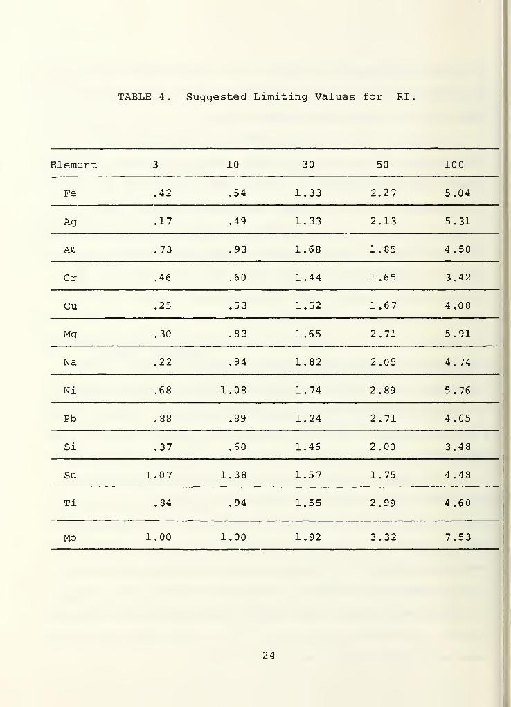
TABLE 4. Suggested Limiting Values for RI

.

Element 3 10 30 50 100

Fe .42 .54 1.33 2.27 5.04

Ag .17 .49 1.33 2.13 5.31

M .73 .93 1.68 1.85 4.58

Cr .46 .60 1.44 1.65 3.42

Cu .25 .53 1.52 1.67 4.08

Mg .30 .83 1.65 2.71 5.91

Na .22 .94 1.82 2.05 4.74

Ni .68 1.08 1.74 2.89 5.76

Pb .88 .89 1.24 2.71 4.65

Si .37 .60 1.46 2.00 3.48

Sn 1.07 1.38 1.57 1.75 4.48

Ti .84 .94 1.55 2.99 4.60

Mo 1.00 1.00 1.92 3.32 7.53

24

the 99.5— quantile of the t-distribution with 9 degrees of freedom

is t qqc = 3.250. The 99% confidence interval for the population

mean then has endpoints X - (3 .250) RI//I0" and X + ( 3 . 250) RI//T0",

where RI is the repeatability index. [The general form for this

100(1-y)% interval is X + t, ,„ RI//n where t, ,- is the- I-y/2 l-Y/2+ v>

100(l-y/2)— quantile from the t-distribution with n-1 degrees

of freedom and n is the sample size, in case it is desired to

change either the sample size or the confidence coefficient.]

If the desired true concentration of the candidate standard is

covered by the confidence interval, accept the candidate standard

as having the correct concentration of the element analyzed. If

the confidence interval does not cover the desired true concentra-

tion then it may not have the correct concentration. To verify

this conclusion an additional 10 burns of the candidate standard

should be made, alternating with burns of the primary reference

standard of the same nominal concentration: candidate-primary-

candidate-primary, etc. Let Y-, , Y~/ ... , Y,Q

be the 10 new

candidate readings with average Y and repeatability index

RI and let Z,, Z_ , ... , ZQbe the 10 primary standard values

with mean Z and repeatability index RIZ

« Both RI and RI

should be no larger than the appropriate entry in Table 4; follow

the instructions above about repeating the burns if either of them

exceed the tabular value. If both satisfy this requirement compute

the joint repeatability index by

S = [j (RI* + Rl2 )]1/2'

25

This in turn can be used to compute a confidence interval for the

difference in true concentration of the candidate and reference

standards as follows: The 99.5th quantile of the t-distribution

with 18 degrees of freedom is t gg5= 2.878. The 99% confidence

interval for the difference in true concentrations then has end-

points Y - Z - (2.878)S//5 and Y - Z + (2 .878) S//5. If this

interval contains zero accept the candidate standard and, if not,

reject the candidate reference standard and conclude its true

concentration is not the desired level. It then must be remixed

or discarded as described above.

NOTE: It is possible that statistical significance and

chemical significance are not identical and this procedure may-

prove too stringent (the criteria may be impossible to meet)

.

That is, in chemical terms perhaps a 30 ppm standard could actually

have a true concentration anywhere between 29 and 31 ppm, say,

without causing any difficulties . Thus a candidate standard should

be acceptable in this case if its true concentration is as low

as 29 or as high as 31 ppm. In the procedure just described, then,

the candidate standard should be initially accepted if 29 or 31

or any value in between is included in the confidence interval for

its true concentration level. (In more general terms, accept the

30 ppm candidate if 30 + A or 30 - A or any number in between

is covered by the confidence interval where A defines the

limits of chemical significance.) If the 30 ppm candidate is

initially rejected, and 10 more burns are alternated with the

26

30 ppm reference standard, accept the 30 ppm candidate if the

confidence interval for the mean difference in the two concentrations

includes -2 or 2 or any number in between. (Again if 30 - A

and 30 + A define the limits of chemical significance, accept

the 30 ppm candidate if -2A or 2A or any number in between is

covered by the confidence interval for the difference.) With these

modifications for chemical significance, the procedure described

should prove a practical and useful way to control the quality of

newly prepared standards.

Origin of Table 4 .

The numbers in Table 4 were computed from data sets supplied

by the TSC as an enclosure to their letter dated July 28, 1977.

Data sets 1 through 9 contain 3 collections of 10 burns of primary

reference standard R-l , by the Pensacola laboratory. RI was

computed for each of these, for each element, giving 3 RI values

for each element-concentration combination. These 3 RI • s were

pooled within each concentration-element combination, using the

formula

RI = V I(RI

1+ RI

2+ RI

3}

*

2 2In theory RI is a constant times a x -random variable with

2 7 degrees of freedom. If we let RI* be the repeatability index

from 10 burns of a candidate standard (some specified element and

2 2concentration) the ratio (RI*) /RI has the F-distribution with

27

9 and 27 degrees of freedom and, with probability .99 this ratio

should not exceed 3.16 or, equivalently , RI* should not exceed

RI /3 .16 . This latter value is given in Table 4. Three entriesP

in Table 4, Si-30, Sn-30 and Mo -3, did not seem reasonable when

calculated from this formula, due to what appeared to be aberrant

results in data sets 1 through 9. These have been adjusted slightl

from what this formula would give. As indicated earlier, the

numbers in Table 4 may be too conservative in some cases . In

such situations larger limiting values for RI have to be chosen.

II. 5. A Numerical Example

Assume the 10 readings gotten for a 30 ppm candidate

standard are as given in Table 5. The average values, X, and RI

values are also listed there, as are the lower and upper 99%

confidence limits computed from the formula discussed above. Note

that none of the RI values exceed the appropriate entries in

Table 4, so the next step is the computation of the confidence

limits (given in Table 5). The confidence limits for Fe , Ai , Ni

,

Pb, and Si do include 30, the nominal level tested, so these

elements appear to be at the correct concentration level. None

of the confidence intervals for the remaining elements, however,

contain 30 so they would all be suspect. Now let us suppose that

chemical common sense dictates the true ppm content could be

anywhere between 29 and 31 (A = 1) and the candidate standard

would be acceptable. This would mean that we want to see if 29

or 31 or any number in between is included between the confidence

28

limits for the remaining elements. With this change, Cr, Sn , Ti

and Mo are now acceptable, but Ag, Cu, Mg and Na are still unaccept-

able. Thus, 10 more burns of the candidate, alternating with 10

burns of the 30 ppm primary reference standard are called for,

with only the readings for Ag, Cu, Mg and Na to be analyzed.

Assume the values in Table 6 result. Again all RI values

are acceptable (compared with entries in Table 4) . Also given in

Table 6 are the values for

=VT(RI„ + RI„)

and the upper and lower confidence limits for the difference in

mean concentration of the candidate and reference standards

using the formula discussed above. Since each confidence interval

includes zero we would conclude that the 30 ppm candidate is

acceptable for all elements . (Granted that chemical common sense

allows A = 1 , we would still have accepted the candidate if the

9 9% confidence limits for Na were, say, -3 and -1, since this

interval includes -2.)

II. 6. Summary of Calibration Standards Testing

a. Carefully standardize the spectrometer using the primary

reference standard at ppm and 100 ppm.

b. Following accepted laboratory techniques make 10 burns

of the candidate standard at each prepared concentration:

3, 10, 30, 50 and 100 ppm.

29

c. For each element and concentration compute the average

110

X = yp- I X. and the repeatability indexxuj=l J

RI = v/ ± E(Xi

- X)2

.

d. Compare RI for each element and concentration with the

appropriate value in Table 4 . If RI exceeds the value

in Table 4 for any element-concentration combination,

restandardize the spectrometer and carefully repeat 10 burns

of the candidate at the same concentration and again

compute RI for each element. If any RI exceeds the

appropriate value in Table 4, the spectrometer should be

checked before proceeding further. After the spectrometer

is again in good working order, start again at a.

e

.

For each element-concentration combination compute the

99% confidence limits for true concentration:

X - (3.250) RI//I0", X + (3.250) RI//T0~. Let CQ

represent

the nominal concentration level and C + A the limits

of chemical significance. If Cn

- A, C. + i or any

value in between lies between the confidence limits

X + (3 .250 ) RI//H", for each element-concentration combina-

tion, accept the candidate standard. If this is not true

for some element-concentration combinations go to f.

30

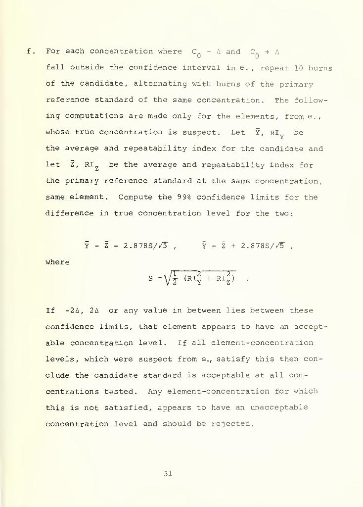
f . For each concentration where Cn

- A and Cn + A

fall outside the confidence interval in e . , repeat 10 burns

of the candidate, alternating with burns of the primary

reference standard of the same concentration. The follow-

ing computations are made only for the elements, from e.,

whose true concentration is suspect. Let Y, RI be

the average and repeatability index for the candidate and

let Z, RI be the average and repeatability index foru

the primary reference standard at the same concentration,

same element. Compute the 9 9% confidence limits for the

difference in true concentration level for the two:

Y - Z - 2.878S//3" , Y - Z + 2.878S//5,

where

S =\/| IHj + RIZ» •

If -2 A, 2 A or any value in between lies between these

confidence limits, that element appears to have an accept-

able concentration level. If all element-concentration

levels, which were suspect from e., satisfy this then con-

clude the candidate standard is acceptable at all con-

centrations tested. Any element-concentration for which

this is not satisfied, appears to have an unacceptable

concentration level and should be rejected.

31

wtnC•H

rC

«

<d

•HT3CCO

U

in

Wffl

o£

•HEh

GW

•Hw

a.

•H2

«3

2

tn2

<

CD

Cm

co in rH m m cyi <tf 10 en t>-

enrH

COen

CN

OmCN00

CNCO

rHro

oro

COro

CNCO

coco

CNCO

CNco

CNro

rH Oco

COCO

i£> rH rH 10 H T \0 in in 00COCN

CN

enCOCN

COrH

Oco

CNro

oro

rHco

Oro

CNCO

rHCO

CN00

Oro

ooo

rHCO

oro

CNCO

m CN <tf UD in CO I> 00 o inCO

enCO CO

o CN00 ro

rHCO CN

CNCO CO

CNco

Hco

Hoo

rHCO

oro

CNro

CN CN in Cn Cn ^O co o <n rHrHH

coCO CN

inen

COCN

O00

oro CM

enCN

oco

enCN

rH00

enCN

H00

OCO

enCN

oco

o <T< r- o ^ CN co ^ 10 ino H

00 oco<*<

CNenCN CN

enCN

00CN

OCO

CT>

CN co CN CNenCN

coCN

oco

m rH CN 10 kD -tf in in CN 00enCN

r^r^

omCOo

oro

CNCO

OCO

enCN

enCN

Oro

oCO

oco

Oro

enCN

oco

enCN

rHco

in -tf <Ti O en CN o rH ro COCOm

enen

oi£>

CN mCO ro

roro

roco

coco

coro

COCO

CN00

0000

coco

CNco CO

r~ <n m O o in en CO CO 00coo CN

•^r^

CNen

0000

CNro

CN00

CNco 00

CNro

coro

CNOO

CNco

coro

CNCO

00oo

o in CN O -* in <7\ in a\ CNrHro

CO CNCO

oCO

ro oococo

ooco

coco

ooro

CNco

coro

CNCO

COco

roro

CNCO

coro

^" CN o O en CN co en 00 oCNco

oo om o

rHro

<Nro

Hro 00

oro

Hco

rHco

CNCO

Oco

Hco

rH00

oco

CNro

<D (N ro co rH O O rH r^ 00 O en10o O

ooo

rHro CN

enCN CN

Oco

Oco

CNCO

<nCN

enCN

oro

enCN

rHCO

in in m 00 O rH co -tf rH ^Omin CO

COCN

CNoo ro

rooo

CN00

roCO

<3*

COcoco ro

COCO

coco

coCO

CNCO co

rH o oo & m H o ^ in ro enco CN

COCN

CNooo

enCN CN

cnCN

rHCO CN

OCO

enCN

Oro

enCN

enCN

oCO

to

<D

en(0

uCD

i

MPtJ

HUu

o

uuCD

ftD

32

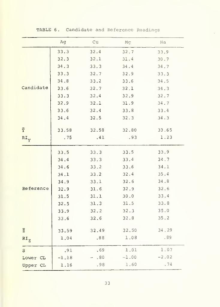
TABLE 6 . Candidate and Reference Readings

Ag Cu Mg Na

33.3 32.4 32.7 33.9

32.3 32.1 31.4 30.7

34.3 33.3 34.4 34.7

33.3 32.7 32.9 33.3

34.8 33.2 33.6 34.5

Candidate 33.6 32.7 32.1 34.3

33.3 32.4 32.9 32.7

32.9 32.1 31.9 34.7

33.6 32.4 33.8 33.4

34.4 32.5 32.3 34.3

Y 33.58 32.58 32.80 33.6 5

RIY

.75 .41 .93 1.23

33.5 33.3 33.5 33.9

34.4 33.3 33.4 34.7

34 . 6 33.2 33.6 34.1

34.1 33.2 32.4 35.4

34.9 33.1 32.6 34 .8

Reference 32.9 31.6 32.9 32.6

31.5 31.1 30.0 33.4

32.5 31.3 31.5 33.8

33.9 32.2 32.3 35.0

33.6 32.6 32.8 35.2

Z 33.59 32.49 32.50 34 .29

RIZ

1.04 .88 1.08 .89

S .91 .69 1.01 1.07

Lower CL -1.18 - .80 -1.00 -2.02

Upper CL 1.16 .98 1.60 .74

33

III. LABORATORY CERTIFICATION

III.l. Introduction

Paragraph 2 of the project order MME-77-006 requires

the development of statistical methodology to evaluate and

certify the spectrometric laboratories participating in the

joint oil analysis program. The evaluation of a laboratory is

to be comprised of three sub-evaluations viz., an evaluation

of the spectrometer performance, a comparison of the laboratory

performance with that of another laboratory that is considered

to have met certification criteria, and an assessment of the

oil analysis evaluator's ability to make correct decisions based

on the results of the analyses.

The methods we present in this paper are applicable for

evaluating the spectrometric analyses results on a single element.

As in the previous chapter, separate evaluations for the different

elements are recommended and, of course, the same statistical

methods are to be used with each element. The same is also true

for different initial concentration levels in the standard oil

samples; a separate statistical analysis for each initial con-

centration level is to be performed. The rest of the discussion,

therefore will apply to the results of repeated independent

34

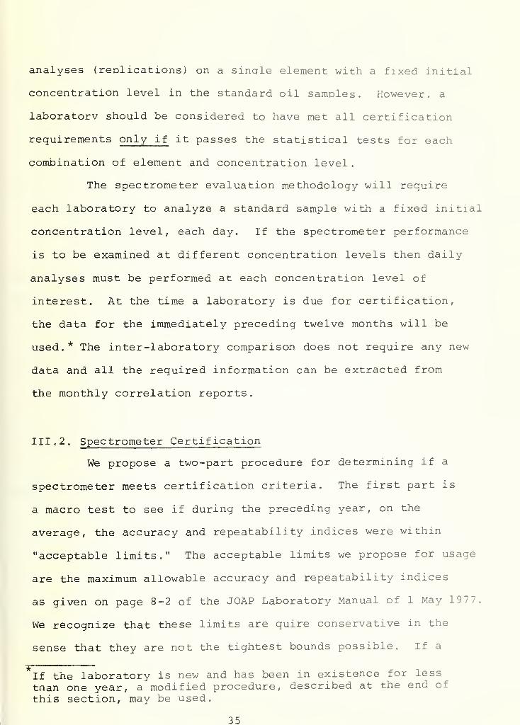
analyses (replications) on a sinale element with a fixed initial

concentration level in the standard oil samoles. However, a

laboratorv should be considered to have met all certification

requirements only if it passes the statistical tests for each

combination of element and concentration level

.

The spectrometer evaluation methodology will require

each laboratory to analyze a standard sample with a fixed initial

concentration level, each day. If the spectrometer performance

is to be examined at different concentration levels then daily

analyses must be performed at each concentration level of

interest. At the time a laboratory is due for certification,

the data for the immediately preceding twelve months will be

used.* The inter-laboratory comparison does not require any new

data and all the required information can be extracted from

the monthly correlation reports.

III. 2. Spectrometer Certification

We propose a two-part procedure for determining if a

spectrometer meets certification criteria. The first part is

a macro test to see if during the preceding year, on the

average, the accuracy and repeatability indices were within

"acceptable limits." The acceptable limits we propose for usage

are the maximum allowable accuracy and repeatability indices

as given on page 8-2 of the JOAP Laboratory Manual of 1 May 197

We recognize that these limits are quire conservative in the

sense that they are not the tightest bounds possible. If a

If the laboratory is new and has been in existence for less

tnan one year, a modified procedure, described at the end of

this section, may be used.

35

better set of bounds can be determined, perhaps based on past

data, they should be used in the tests described herein. Part

two is a micro test comprised of twelve separate analyses of

the monthly results; this test is essentially a test for

consistency.

Let X.., i = 1,2, ...,12; j = 1,2,... be the results

of the spectrometric analyses for a specified combination of

element and concentration level. The subscript i ranges

over the twelve months and the subscript j represents the

working days within each month. Thus, the total number of X's

will be equal to the number of working days for the year. Let

n. = number of data points for the i month

• 12N = y n. = total number of observations

i=lx

12 i

XJ £ X. ./N = average for the year

i=l j=l 13

TO n •

212 i

2S =

I I (X. .- X) /(N-l) = sample variance for the jjf

i=l j=l X J

l_i

Q= initial concentration level

Afl

= maximum allowable accuracy level

Rq = AQ/2 = maximum allowable repeatability level

a = .05 = significance level or Type 1 error probability

36

2X

ZQ5

= -1.645 = tabulated 5 percentile of the

standard normal distribution

Zg75

= 1.96 = tabulated 97.5th

percentile of the

standard normal distribution

2 i r ~|2 ,

05 N-l=

2" I" 1 - 645 + ^2N-3 = approximate 5 percentile

of a chi-square distri-

bution with N-l degrees

of freedom

t q_ 5 q = 2.262 = 97.5 percentile of the student's

t-distribution with 9 degrees of freedom

We assume that the X. .'s are normally distributed with an unknown

2mean value y and an unknown variance a . Previous studies have

shown that, as a general rule, the results of spectrometric

analyses tend to be normally distributed.

a. Macro Test . This test consists of statistically

establishing whether or not, the true accuracy indexI y-y^ I and

the true repeatability index a are below the maximum values

An and R_, respectively. We first compute a 95% upper con-

fidence bound for a2

as [(N-l)S /X >0 5,n-1 ] (that is,

[Q2

<(N-DS 2

X. 05, N-l J

= .95

2 2Since it is required that a < R we can conclude, with about

95% confidence, that the repeatability index is within acceptable

37

bounds provided that

(N-l)2

R2

2N "0

X .05

The chance that this procedure will result in a conclusion that

the repeatability index is unacceptable, when in fact it is,

is about 5%. Next, we obtain a 95% confidence interval for

y as X + Z Q -c(S//N) (that is,- ".975

]

X " Z .975 -^ < V < X + Z_975 —

The maximum acceptable accuracy index is An

, which implies that

I y-U n Imust be less than A

flor equivalently y must satisfy

the inequality constraint

yQ

- AQ

< y < yQ

+ AQ

(2)

A combination of (1) and (2) will provide the criterion for

acceptability of the accuracy index viz., conclude that the

accuracy index for the spectrometer meets the certification

criterion if

|X - u | < AQ

- (1.96) -§-

The probability of wrongly concluding that the accuracy

index is unacceptable is about 5%. If both the accuracy index

38

and the repeatability index are found to be acceptable, the macro

test has been met and we proceed to the next stage.

b. Micro Test . This is a procedure to check whether,

on a monthly basis, the spectrometric analyses results are consistent

and that there are no significant fluctuations from month to

month. We do this by computing twelve 9 5% confidence intervals

for the unknown mean \i , based on a sample of size 10 observa-

tions for each month. From among the n. observations for the

i month a sample of size 10 is selected; we suggest that every

second observation starting with the second working day of each

month be selected. As long as the spectrometric laboratories

are not aware of the selection process it should not result in

any systematic bias creeping in. It may happen that for certain

months (February, for example) the selection scheme will not

result in ten samples. If this is the case, additional samples

to make up the difference should be taken at random from the

remaining data for the month. Let Y.,, Y . ,, , ... , Y. , n3 ll i2 'i,10the ten measurements sampled for the i month and let

10Y. = J Y. . /10 be the sample mean1

j=l ^

be

and

210

S. = 7 (Y. .- Y.)/9 the sample variance.

1 jii ^

39

The 95% confidence interval for y, for the i month will then

be

S. S.

Y. - (2.262) —— < \i < Y. + (2.262) —— , i = 1,2,...,1

/TOX

/TO

As in the case of the macro test, we conclude that the accuracy

index for the i month meets the certification criterion if

Y. - ul < An - (2.262) —i-100 /TO

,This procedure will wrongly conclude that the results for a mont

do not meet certification criteria about 5% of the time. Now,

let us examine the results of the "acceptance sampling" scheme

for the twelve months in question. If the spectrometer

performance is consistent throughout the year, the number of

monthly acceptance sampling tests that will lead to a rejection,

has a binomial distribution; the parameters of the distribution

are m = 12 and p = .05. An examination of the binomial

tables shows that about 9 8% of the time at least 10 monthly test:

should result in acceptance. Thus, the micro test will conclude

that the spectrometer does not meet the certification criterion

if the number of "acceptance tests" that lead to acceptance is

less than 10

.

jo.

40

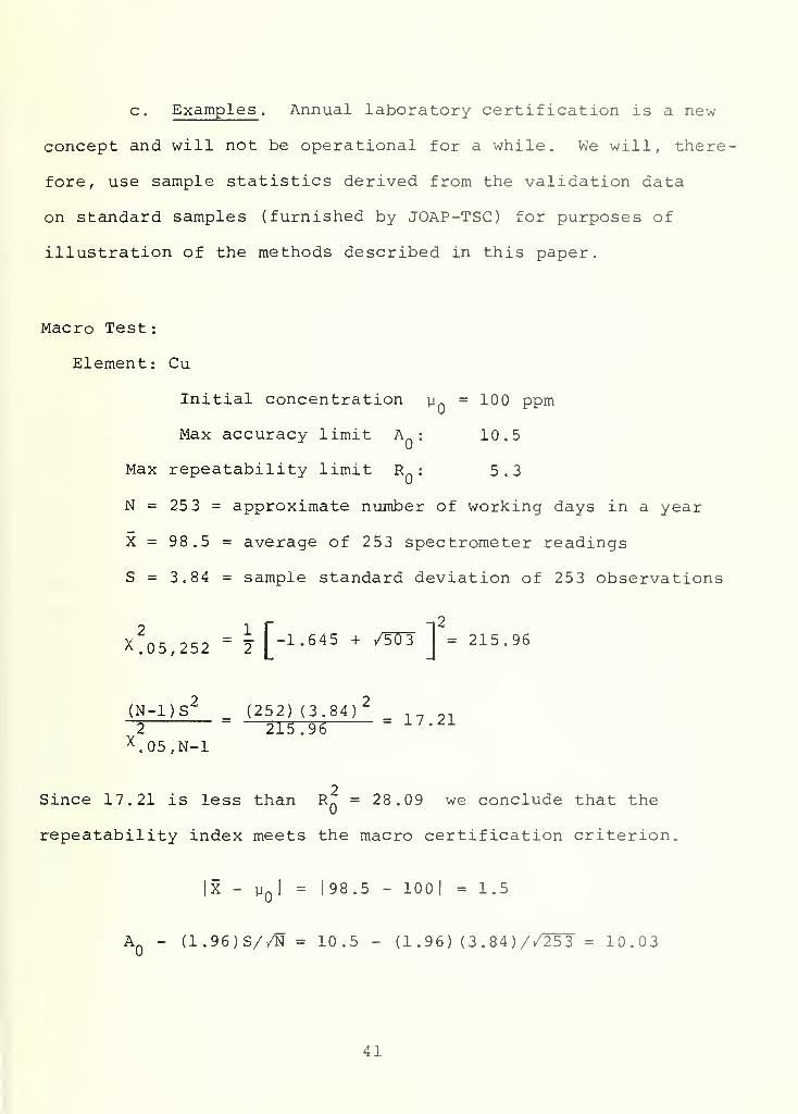
c. Examples . Annual laboratory certification is a new

concept and will not be operational for a while. We will, there-

fore, use sample statistics derived from the validation data

on standard samples (furnished by JOAP-TSC) for purposes of

illustration of the methods described in this paper.

Macro Test:

Element : Cu

Initial concentration p_ = 100 ppm

Max accuracy limit Afi

: 10.5

Max repeatability limit R : 5.3

N = 25 3 = approximate number of working days in a year

X = 98.5 = average of 253 spectrometer readings

S = 3.84 = sample standard deviation of 253 observations

x'o5,252 " y [-1-645 + /5uTi2

= 215.96

(N-l)S2

_ (252) (3.84)_^_ = 1? 2±2

'

215.96X .05,N-1

2Since 17.21 is less than Rn

= 28.09 we conclude that the

repeatability index meets the macro certification criterion

|X - uQ|

= |98.5 - 100 ! = 1.5

AQ

- (1.96)S//N = 10.5 - (1.96) (3.84)//25~3 = 10.03

41

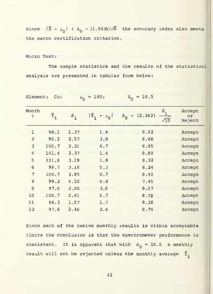
Since I X - y. I< A

fl

- (1.96)S//N the accuracy index also meets

the macro certification criterion.

Micro Test:

The sample statistics and the results of the statistical

analysis are presented in tabular form below:

Element: Cu; y = 100; AQ

= 10.5

Month S. Accepti Y.

ls.1

|Y\ - yQ| A

Q(2.262)

lor

Reject/To"

1 98.1 1.37 1.9 . 9.52 Accept

2 96.2 2.57 3.8 8.66 Accept

3 100.7 2.31 0.7 8.85 Accept

4 101.4 2.37 1.4 8.80 Accept

5 101.8 3.19 1.8 8.22 Accept

6 99.7 3.16 .3 8.24 Accept

7 100.7 2.95 0.7 8.40 Accept

8 99.2 4.26 0.8 7.45 Accept

9 97.0 2.00 3.0 9.07 Accept

10 100.7 2.41 0.7 8.78 Accept

11 98.3 1.57 1.7 9.38 Accept

12 97.6 2.46 2.4 8.74 Accept

Since each of the twelve monthly results is within acceptable

limits the conclusion is that the spectrometer performance is

consistent. It is apparent that with An

= 10.5 a monthly

result will not be rejected unless the monthly average Y.

42

differs from \iQ

by a large amount; an examination of the

validation data for standard samples shows that large differences

occur very rarely, if at all. A more sensitive procedure would

result if the maximum accuracy deviation is modified to

A' = A_/2 = 10.5/2 = 5.25. If this change is adopted the results

of the macro test will be unaffected since A' - (1 .96) S//N = 4 . 78

and | X — y qI

is less than 4.78. For the micro test the monthly

results for the second month will be unacceptable since

|Y2

- p I= 3.8 is greater than A^ - (2.262)S //lO" = 3.41.

However, because only one out of the twelve monthly tests leads

to rejection the micro test would result in the conclusion that

the spectrometer is consistent. Even if An

is changed to A',

the maximum repeatability index Rn

= Ar>/^ must be left unchanged

since it is already a reasonably tight bound. It should be

pointed out that in order to qualify for certification a labo-

ratory has to pass each of the statistical tests for all combi-

nations of elements and concentration levels for which data has

been collected. With 20 elements and 5 concentration levels

the number of combinations is 100. If A' = A./2 is used in

place of An

itself, as the maximum accuracy limit, this will

definitely increase the chance of at least one rejection out

of the 100 combinations.

Some of the newer laboratories would have been in

existence for less than a year. In these cases, full year's data

will not be available and the tests will then have to be modified.

43

As an example, if data is available for six months or more

both the macro and micro tests can still be performed. For

2the macro test the parameters N, X nc N_i quoted earlier

should be suitably modified. The parameter for the micro

test will have to be replaced with the actual number of

months for which data is available and a new "acceptance

number" has to be determined from an examination of the

tables of the binomial distribution. We recommend that the

micro test not be used if the number of months is less than

6 since we believe that the test will not be very sensitive

in this case.

III. 3. Interlaboratory Comparison

As indicated in the introduction the laboratory certi-

fication scheme is to include a comparison of the performance

of a laboratory that is to certified with that of another

laboratory that has previously received certification. We

believe that it is preferable to use a single laboratory such

as the Pensacola laboratory as a standard against which all

others are compared. The advantage of doing so is that the

performance of the standard laboratory can be monitored on a

regular basis to maintain a high performance level; besides,

comparing all laboratories against a single standard laboratory

44

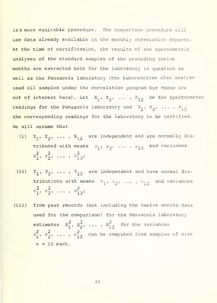
is a more equitable procedure. The comparison procedure will

use data already available in the monthly correlation reports.

At the time of certification, the results of the spectometric

analyses of the standard samples of the preceding twelve

months are extracted both for the laboratory in question as

well as the Pensacola laboratory (the laboratories also analyze

used oil samples under the correlation program but these are

not of interest here). Let X, , X_ , . . . , X, „ be the spectrometer

readings for the Pensacola laboratory and Y, , Y2

, ... , Y,-

the corresponding readings for the laboratory to be certified.

We will assume that

(i) X,, X,,, ... , X,2

are independent and are normally dis-

tributed with means y, f \i , .,. , y,2

and variances

2 2 2°1' °2' '" ' °12 ?

(ii) Y, , Y2 , ... , Y,

2are independent, and have normal dis-

tributions with means v, , v,,, ... , v,2

and variances

2 2 21 ' 2 ' • • • ' 12'

(iii) from past records (not including the twelve months data

used for the comparison) for the Pensacola laboratory

2 2 2estimates S, , S

2 , ... , S,2

for the variances

2 2 2a,, a

2 , ... , a, ^ can be computed from samples of size

n = 10 each.

45

2The reasons for letting the ji's, v's and a 's be different

for different months is to allow for the possibility that the

standard samples have different initial concentration levels

and consequently non-identical means and variances . It is to

2be noted that the number of distinct y ' s , v's and a 's

is equal to the number of distinct concentration levels in the

correlation samples.

The implication of the assumption that both the X's

and the Y's have the same variance within each month is that

the emphasis in the interlaboratory comparison is on the

accuracy and not so much on repeatability provided, of course,

the repeatability indices are not too far apart.

With the above assumptions, the quantities

(X. - Y. ) - (\i. - v. )

1 i __i i_1 /Is.

l

are independent and each t. has a student's t-distribution

with n-1 = 9 degrees of freedom. If the performance of the

laboratory to be certified is the same as that for the

Pensacola laboratory, y. will be equal to v.. In this case,

it can be shown that P[|x. - Y. I > 2S.] = .20 approximately.

In other words, if the means for the two laboratories are equal,

the observed readings X., Y. will differ by at least two stand,

deviations about 20% of the time. Now, consider the twelve

46

absolute differences |x. - Y . I , i = 1,2,..., 12. The number of

times these differences will exceed twice the corresponding standard

deviation S. is a binomial random variable with parameters

m = 12 and p = .20. From the binomial tables, it is observed

that the number of differences that exceed twice the standard

deviation will be less than or equal to five with probability

.98; equivalently, the chance of observing six or more pairs

that differ by more than two standard deviations is .02. This

then provides a comparison test as summarized below:

Step 1 : From past records for the Pensacola laboratory compute

2 2 2the sample variances S-,, S~, ... , S,- using a sample

of size 10 for each computation. The number of different

2S. to be computed is equal to the number of distinct

concentration levels used in the correlation samples.

If all correlation samples have the same concentration

level only one S needs to be computed. From a

practical point of view, the trimmed sample variances

already available in the correlation reports may serve

the purpose and may result in the saving of some labor.

We believe that this change will not severely affect

tne validity of the statistical procedure.

Step 2 . Compute |X. - Yi

I, i = 1,2,..., 12.

47

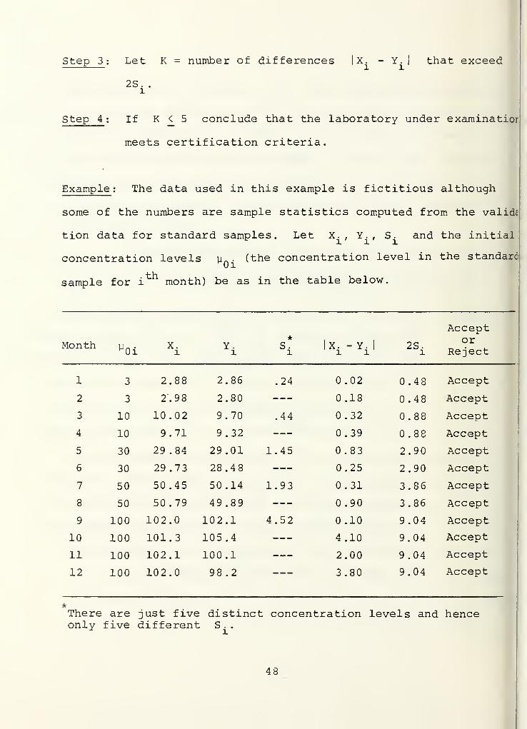
Step 3

:

Let K = number of differences X. - Y.l l

that exceed

2S. .

l

Step 4 ; If K <_ 5 conclude that the laboratory under examinatior

meets certification criteria.

Example: The data used in this example is fictitious although

some of the numbers are sample statistics computed from the validc

tion data for standard samples. Let X.. Y., S. and the initialr illu . (the concentration level in the standardM0i

concentration levels

sample for i month) be as in the table below.

Monthl

0iX.l

X. - Y.l l

2S

Acceptor

Reject

1 3 2.88 2.86 .24 0.02 0.48 Accept

2 3 2.9 8 2.80 0.18 0.48 Accept

3 10 10.02 9.70 .44 .32 0.88 Accept

4 10 9.71 9.32 0.39 .88 Accept

5 30 29.84 29.01 1.45 0.83 2.90 Accept

6 30 29.73 28.48 0.25 2.90 Accept

7 50 50.45 50.14 1.93 0.31 3.86 Accept

8 50 50.79 49.89 0.90 3.86 Accept

9 100 102.0 102.1 4.52 0.10 9.04 Accept

10 100 101.3 105.4 4.10 9.04 Accept

11 100 102.1 100.1 2.00 9.04 Accept

12 100 102.0 98.2 3.80 9.04 Accept

There are just five distinct concentration levels and henceonly five different S .

.

48

There are zero rejections, so we conclude that the laboratory

passes the comparison test.

The comparison test described above is applicable to

most of the spectrometric laboratories participating in the

Joint Oil Analysis Program. The requirement is that a laboratory

is to have participated and analyzed standard samples under

the correlation program for at least twelve months prior to

the time the laboratory is due for certification. As indicated

earlier the advantage is that no new data need be collected

and the monthly correlation reports provide all the necessary

information. Some of the newer laboratories, such as the

Fort Riley laboratory, will not meet the requirement. We

recommend that, in these cases, the following modified approach

be adopted. JOAP-TSC will prepare twelve pairs of standard

samples with a mixture of concentration levels; we suggest

that the twelve pairs be comprised of two pairs each at

3, 10, 30 and 50 ppm and four pairs at 100 ppm concentration

level . For each pair one sample will be analyzed at Pensacola

and the other by the laboratory to be certified. The

statistical analysis will be on the same lines as before,

i.e. as given in Steps 1 to 4 above.

49

III. 4. Evaluation Testing

The final subtask is the design of a test to be

administered to the evaluators that are assigned to the

spec trometrie laboratories. The JOAP Laboratory Manual dated

1 May 1977 provides decision making guidance tables to aid the

evaluator in his decision making process. Separate tables are

provided for each type of equipment and contain numerical

criteria relating the oil sample wearmetal concentration to the

expected health of a component of the equipment. The recommended

decisions are based on comparisons of the results of a used

oil sample with that of a previous sample. The types of

decisions an evaluator can make are (i) not to take any action;

(ii) call for a more frequent sampling schedule; (iii) call

for an immediate additional sample; (iv) recommend a maintenance

action. The losses resulting from incorrect decisions by

the evaluator can be quite high. A JOAP failure, i.e., an

equipment that is being monitored by JOAP fails prior to detectio

by JOAP can result in a loss of the equipment. Similarly, a JOAP

miss, i.e., a JOAP recommended maintenance action which finds

no discrepancies can be expensive. It is, therefore, very

important that an evaluator be quite conversant with the basic

facts about wearmetal concentrations and also have sufficient

experience with analyzing sample results to look for trends and

shortrun features such as a sudden rise in concentration levels

right after overhaul . We suggest that the examination be in

50

two parts. The first part consists mostly of multiple choice

questions which will test the basic knowledge about wearmetal

concentrations that is critical for the various types of

equipment being monitored. The second part will present actual

historical data to illustrate the kinds of trends and the

ambiguities that an evaluator will encounter. The test will

examine his performance as gauged by the number of correct

decisions made.

A set of sample questions testing basic knowledge are

presented below.

(1) Spectrometric analysis will not detect

a) worn, misaligned or scored gears

b) broken piston rings and bands

c) failures due to fluid starvation

d) loose or defective valve guides

e) chips or wearmetal particles visible to the eye

(2) Explain in two or three sentences the effect of each of

the following on the integrity of spectrometric analyses

a) contamination

b) electrodes

c) calibration standards

d) electrolytic corrosion

e) new or recently overhauled components

51

(3) Briefly describe the six steps to be followed in evaluating

the sample results of incoming oil samples.

(4) If for aircraft types T-lA, T-33A, T-33B or QT33A, a sudden

increase in Fe and Mg is observed the recommended action

is to inspect

a) accessory drive assembly oil pump

b) main starter housing assembly

c) main bearing seals

(5) For F-101/F-102 aircraft the most significant and critical

wearmetal is

a) Fe

b) Mg

c) Cu

d) Ag

e) Cr

(6) For F-84, B-57 aircraft the most significant wearmetal is

a) Fe

b) Mg

c) Cu

d) Ag

e) Cr

52

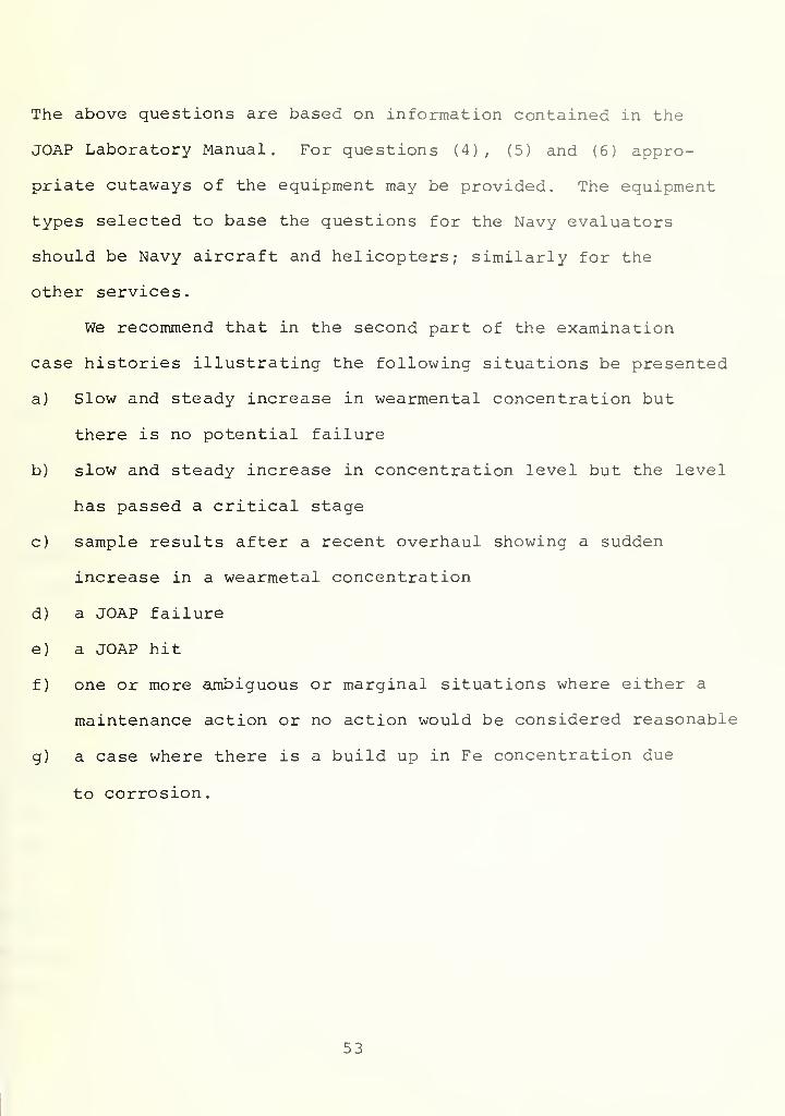
The above questions are based on information contained in the

JOAP Laboratory Manual. For questions (4), (5) and (6) appro-

priate cutaways of the equipment may be provided. The equipment

types selected to base the questions for the Navy evaluators

should be Navy aircraft and helicopters; similarly for the

other services.

We recommend that in the second part of the examination

case histories illustrating the following situations be presented

a) Slow and steady increase in wearmental concentration but

there is no potential failure

b) slow and steady increase in concentration level but the level

has passed a critical stage

c) sample results after a recent overhaul showing a sudden

increase in a wearmetal concentration

d) a JOAP failure

e) a JOAP hit

f) one or more ambiguous or marginal situations where either a

maintenance action or no action would be considered reasonable

g) a case where there is a build up in Fe concentration due

to corrosion.

53

IV. GRAPHITE ELECTRODES

IV. 1. Introduction

The accuracy of readings produced by a batch of

electrodes is of primary importance in judging the accept-

ability of the batch for use in the oil analysis program.

The repeatability characteristics of the electrodes are also

of some importance in judging acceptability. If a batch of

electrodes scores badly on repeatability one can expect a

number of spurious readings, including ones which may be too

low (possibly missing a significant increase in some contam-

inant in a used oil sample) and ones which may be too high

(possibly indicating a high contaminant reading when the

level has not changed) . Thus it is suggested that both

repeatability and accuracy be considered in judging the

acceptability of a new batch of electrodes.

The judgments of whether the new batch of electrodes

is acceptable with respect to accuracy and repeatability can bes

be made by comparison with readings gotten, on the same pre-

pared oil sample, by using electrodes from a previously

accepted batch. It is suggested that the elements of interest

be considered one after another. For convenience it is assumed

that a 10 ppm primary reference standard is used. A different

oil standard could be used if desired.

54

IV . 2 . Acceptance Criteria for Graphite Electrodes

The suggested procedure calls for analyzing the spectrometer

readouts one element at a time, to ensure that the electrodes are

uncontaminated by any element of interest. To distinguish between

the readings gotten with the new batch of electrodes versus those

from the previously accepted batch we shall use a double subscript,

the first subscript equalling one if the reading is made with an

electrode from the new batch and this first subscript equals two

if the reading is made with an electrode from a previously

accepted batch. The second subscript distinguishes between the

several readings made with the same type of electrode. We shall

assume n, samples are analyzed with the new electrodes and n2

with the old. (There is no special reason that we would have

n, ^ n_; the formulas presented allow for either n, = n_ or

n, ^ n2

-

)

Thus the element readings from the new batch are

X, , , X, „. ... , X, and from the previously accepted batch11' 12 In, c

they are X ,, X2

, ... , X2n

. For each set of readings we

can compute the sample means

:

new batch X = -— (Xn

, + X, . + • •• + X n )1 n^ 11 12 In,

previously accepted X = ±- (x o , + x oo + • • • + x„ )z &2 ^ 1 22 2n_

and the repeatability indices:

55

(x21

-x2

)

2+( x

22-x

2)

2+ ... + ( x2n

-xpreviously accepted s

9= \l - 2

n2-l

The comparison of the two sets of readings is done in 2 steps.

First we shall test the hypothesis that the repeatability index

for the new batch does not exceed the index for the old.

Granted this is accepted, we then will test the hypothesis that

the mean reading for the new batch does not exceed the mean

reading for the old.

To test that the new repeatability index does not

2 2exceed the old we compute s../s and compare this ratio

with a value from an F table with n, -1 and n o~l

degrees of freedom. Which entry to use is determined by

the value desired for the probability of rejecting the new

batch because of bad repeatability, when in fact it has an

acceptable repeatability index. Suppose we set this prob-

ability at .01 and denote the tabular entry by F OQ . We. y y

then conclude the new batch is acceptable with respect to

2 2repeatability if s t/s 2 — F 99 ; otnerwi se we conclude it

is not. '

56

2 2Granted that we find s i/ s 2 1 F 99 ' we then proceed

to test the equality of mean readings. We first compute the

combined repeatability index (pooled standard deviation) by

2 2(n

1-l)s

1+ (n

2~l)s

2S = \ I

; tP V n, + n - 2

We then compute the test statistic

Xl " X

2

PV ni

n n

which is compared with an entry from the t-distribution table.

Again the entry to use is determined by the probability

desired of concluding the new batch is not acceptable in

accuracy, when in fact, it is acceptable. Suppose we set

this probability at .01; we need the quantile tgg5

from the t-distribution with (n, + n_ - 2) -degrees of freedom

We then say the batch is acceptable with respect to accuracy

if

Xl

" X2

s^FT1< t- .995 '

otherwise we reject the batch because of poor accuracy

57

As described, this test is "two-tailed" and the new

batch of electrodes would be declared unacceptable if X, -X^

gets too large either positively or negatively. A large positive

difference may be rightly attributed to possible contamination

of the new batch of electrodes. A large negative difference,

however, would seem to indicate that the previously accepted

batch of electrodes contains a higher concentration of the

element being analyzed than does the new batch. Logically

one would not want to reject the new batch in this case. If

this case occurs for one or more elements the procedure

followed should be closely examined and the possibility of

contamination of the old batch should be investigated.

This procedure is illustrated numerically below,

assuming n, = n_ = 15 samples analyzed with both the new

and old electrodes. Although they are not written in that order,

it is assumed that the analyses with the old and new electrodes

are done alternately, to protect against a possible drift of

the spectrometer during the period of analysis. The sample

sizes of n, = n_ = 15 are used for illustration only. In

acceptance testing of large batches of material MIL STD 105D

should be consulted regarding appropriate sample sizes. The

assumed readings (for 10 ppm standard) are

58

Xlj X

2j

9.5 9.5

10.1 8.8

9.8 9.1

9.4 8.9

9.6 9.2

9.6 9.3

9.5 9.5

10.1 9.4

9.7 9.4

9.7 10.1

10.0 9.3

10.2 9.0

10.0 9.8

10.0 9.5

9.7 9.4

We find X, = 9.79, X2

= 9.35, s, = .255, s2

= .333, and thus

2sl4= .58 ;

S2

Since Fg q

is about 3.5, with n, -1 = 14 and n?~l = I 4

degrees of freedom, we would accept the new batch for

repeatability. We then compute

59

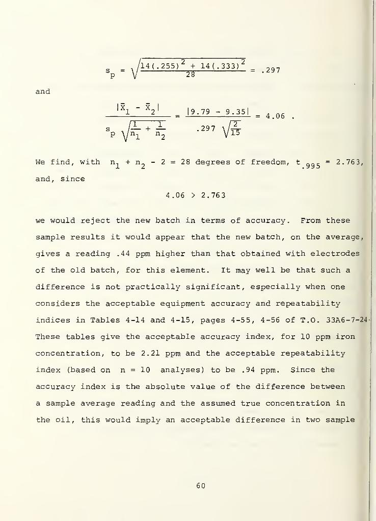
and

s = ,/l4(.255) 2

^ 14(.333)2

. ^p V 28

XlI

*2

'

= '9 ' 79 - 9 - 3^ = 4.06 .

sA/T7I .297 a/^

p A/n, n V 15

We find, with n. + n„ - 2 = 28 degrees of freedom, tg g g

= 2.763,

and, since

4.06 > 2.763

we would reject the new batch in terms of accuracy. From these

sample results it would appear that the new batch, on the average,

gives a reading .44 ppm higher than that obtained with electrodes

of the old batch, for this element. It may well be that such a

difference is not practically significant, especially when one

considers the acceptable equipment accuracy and repeatability

indices in Tables 4-14 and 4-15, pages 4-55, 4-56 of T.O. 33A6-7-24

These tables give the acceptable accuracy index, for 10 ppm iron

concentration, to be 2.21 ppm and the acceptable repeatability

index (based on n = 10 analyses) to be .94 ppm. Since the

accuracy index is the absolute value of the difference between

a sample average reading and the assumed true concentration in

the oil, this would imply an acceptable difference in two sample

60

averages of 2(2.21) = 4.42 ppm. The acceptable pooled standard

deviation for two samples of size 10 then would be

s _,/ 9(-94)2

+ 9(.94)2

94P V i 8

and the implied acceptable value of the t-statistic would be

4.42= 10.51

.94 /2/10

With 18 degrees of freedom, a random variable with tne

_7t-distribution will exceed 8.115 with probability 10 . The

implied acceptable t value of 10.51 above would occur with

-7probability considerably less than 10 . This means that,

if the two electrode batches are uncontaminated, there is

less than 1 chance in 10 million of the t-statistic being

this large. Therefore the tabled values mentioned do not seem

to provide reasonable values for deciding the acceptability

of electrode batches. Even if one allows the difference in

mean readings of two samples of size 10 to be only 2.21, the

table accuracy index value, this still implies an acceptable

t-value of

2 21 = 5.2694 /27Tb"

61

which has probability of about .00005 of occurring if both

batches are uncontaminated . If the new batch is contaminated,

and the old is not, this magnitude for the t-statistic is

much more likely to be observed. Thus values of t this

extreme should not be called acceptable, because of the size

of the associated large probability of accepting a contaminated

batch.

It still may be desirable to allow, say c ppm difference

in apparent content of the contaminant before rejecting the

new batch. This may be accomplished as follows: If X, > 5L

accept the new batch unless

X - X - c_ _ > t| 995

s .,/JL +i

PVn 1n2

and if X, < X_ accept the new batch unless

X, - X + c_ _ < _t

,,/nr -

995

p\/n, n

With the above values X, = 9.79, X- = 9.35, s = .297,1 2 P

n, = n_ = 15 and with c = 1 , we have X, > X_ and thus

we compute

62

9.79 - 9.35 - 1 _ . _—— = -5.16

.297 /2/15

which is smaller than 2.763 so the new batch would be accepted.

There are two possible errors which could be made in

considering a new batch of electrodes: A contaminated batch

may be accepted (called Type II error) or a good batch may

be rejected (called Type I error) . For any two specific sample

sizes n, and n the smaller that one makes the probability

of type I error the larger the probability of the type II

error, and vice versa. Because of this one may not want

to use such extremely small probabilities of type I error as

would be suggested by the values in Tables 4-14 and 4-15 of

T.O. 33A6-7-24-1 mentioned earlier.

Sample sizes of at least n, = n2

= 30 and the probability of

rejecting a good batch set at .01, for both the F and t

statistics used, should provide a useful acceptance criteria.

Mil STD 105D should be consulted for reasonable sample sizes

in acceptance sampling of large batches of material.

This 2-stage test, or its adaptation, should be carried

out in turn for each element of interest. If the new batch

is rejected for any one or more elements, these electrodes

should be declared unacceptable.

63

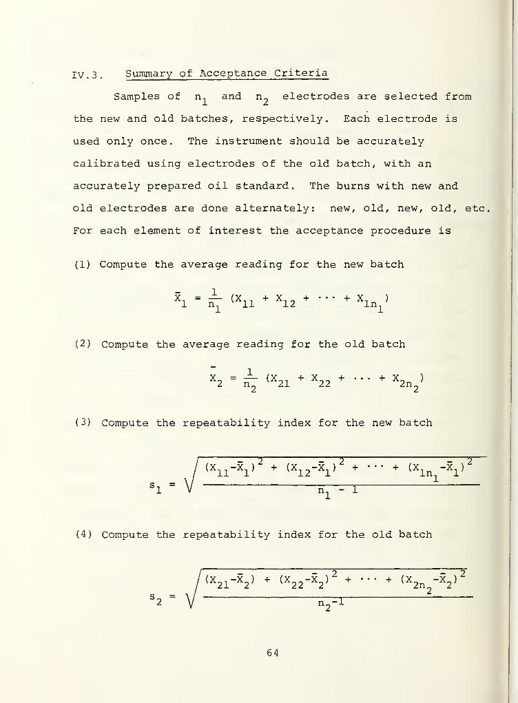
IV. 3. Summary of Acceptance Criteria

Samples of n, and n_ electrodes are selected from

the new and old batches, respectively. Each electrode is

used only once. The instrument should be accurately

calibrated using electrodes of the old batch, with an

accurately prepared oil standard. The burns with new and

old electrodes are done alternately: new, old, new, old, etc

For each element of interest the acceptance procedure is

(1) Compute the average reading for the new batch

x. =f (xn +x + ••• +X )

1 n, 11 12 In,

(2) Compute the average reading for the old batch

X2 =

i7J<X

21+ X

22+ ••• + X

2n2

>

(3) Compute the repeatability index for the new batch

(4) Compute the repeatability index for the old batch

64

2 2(5) Compute s t/s 2 and compare with F , n -1, n -1 degrees

of freedom. These may be found in "Tables of Common

Probability Distributions," P.W. Zehna, D.R. Barr,

Naval Postgraduate School Technical Report NPS 55ZeBn 0091A,

pages 16-21 or some equivalent source. Use column

n = n, -1 (interpolate if necessary), major row m = n„-l,

2 2minor row label .99. If s,/s~ >_ F .,, reject the new

? 2batch for poor repeatability. If s^/s_ < F „« , go on to 6

.

(6) Compute the combined repeatability index

(7) Compute

Xl " X

2

P\/ nl

n2

(8) Find t gq[- from column .995, row n = n1

+ n2

- 2,

page 23, in "Tables of Common Probability Distributions,"

P.W. Zehna, D.R. Barr, Naval Postgraduate School Technical

Report NPS 55Ze Bn 0091A, or some equivalent source.

If n + n2

- 2 > 30, use t 995= 2.575.

65

(9) If

X -X|< t

.995n 1s . +p

/ni

n2

the readings are acceptable for this element. Go on to

analyze another element, starting at 1.

(10) If

X, - X|

> t.995

P\l n1n2

the performance of the new batch of electrodes is

unacceptable.

IV . 4 . A Statistical Test to Evaluate Trace Metal Content

of Graphite Electrodes as Determined on the

A/E 35U-3 Spectrometer .

Just as with the acceptance criteria described above,

the evaluation of the trace metal content of the new graphite

electrodes is most appropriate measured relative to readings

gotten with electrodes of known quality. The procedure for

accomplishing this is described below.

66

Assume n burns of the selected reference standard

(say, 10 ppm) have been made with electrodes from the

new batch. The discussion is pertinent for each

element in turn and we let X, , , X, „,.... X, be11 12 In,

the spectrometer readings for iron, say, and let X,

and s, be the average and repeatability index,

respectively, for these n, . Let X-,, X~~,...,X~-* 1 21 22 2n„

be the spectrometer readings for this same oil

standard using electrodes from a previously accepted

batch. The average reading using the previously

accepted electrodes then is X„ and their repeatability

index (standard deviation) is s_. A good measure of

the excess iron trace metal content in electrodes of

the new batch versus those previously accepted, is

given by X, - 5L . It is easy to compute an interval

with the property that we know how likely it is that

the true average excess of the iron reading (new batch

versus old) is included in the interval. This again

requires values from the t-distribution and requires

the pooled standard deviation (repeatability index)

:

Sp V n + n_ - 2

If we want an interval which we are 100y% sure includes

the true excess, we need t* = t from the t-distributionY

67

with v=n, + n?

- 2 (row v, column y) . Then we can

be 100y% sure the true average excess does not exceed

X, - X + t*s W— + —1 2 p y n

1n2

This is illustrated below.

Let us use the same data that was used in the

acceptance criteria discussion above. Thus we have

n, = n. = 15, X. = 9.79, X. = 9.35, s = .29712 1 2 P

and we found t ggc = 2.763 with 28 degrees of freedom

Then we can be 100y% = 99.5% sure the excess iron

contaminant in the new batch, relative to the old, is

no larger than

9.79 - 9.35 + 2.763(.297) \f^ = .74 ppm,

IV . 5 . Variance Contributed by Electrode

To identify the variance contributed by the new batch

of electrodes again let us discuss estimation on an element

by element basis. We shall explicitly discuss the procedure

and formulas for iron, say, with the understanding that the

same procedure and formulas can be applied in turn for copper,

aluminum, magnesium, etc.

68

We assume n, electrodes have been selected from the

new batch, each to be used in analyzing a sample of the same

oil, say a prepared standard containing 10 ppm of iron. Let

X, , , X-,-,..., X, be the n iron readings produced by the

spectrometer using these electrodes from the new batch. We

also assume we have n electrodes from a previously accepted

batch, each used to analyze a sample from the same oil standard

Denote these iron readings by X21' X22'**'' X 2 * T^e tota -'-

variance , then of these n, + n„ iron readings is a constant

times the sum of the squares of each individual reading less

the overall mean:

2 n

.

i=l i=l il

where the overall mean is

2 n±

X = n I n I I X' • 'n

l+ n

2 i=l j=l ^This total sum of squares can be partitioned into two parts

2 n . 2 n

.

_ 2J- - o 1

~> nTn o X,-X„

I I (X -x)2

=I I (x..-x.)

2+ \ 2

+\2

i=l j=l 1: i=l j=l ^ 1 nl

+ n2

where

1 " RT IXlj '

X2 " X

2j1 3 3

69

are the average readings for the two electrodes . The first

of these

2ni

nl

n2

I I (x -x) 2 =I (X -x) 2

+ I (X -X) 2

i=l j=l ^ xj=l 1D L

j=l ZJ z

is just the sum of squares of the readings for each electrode

about its own average value: part of the variability of the

n, + n?

readings is given by the variability within read-

ings by the same electrode type. The remaining term

nln2 - - 2

(X, - x rn, + n v

i 2

is a constant times the square of the difference between

the two averages: the remainder of the variability in the

n-. + n readings is related to the difference in average

readings of the two electrode types. This partition of the

total sum of squares is frequently called an analysis of

variance; it breaks the total variance into parts which can

then be compared. The discussion of acceptance criteria

in paragraph c above actually is using this same partition

although it is not described in that way.

Isolation of the variance due to the electrode type may

be done in a relative sense as follows: Let us assume that

the variance of a reading, using an electrode from the new

batch is

2 2V[X

1.] = a + a

1

70

2where a is the variance due to the instrument, oil standard

2used, etc., and a^ is the contribution from the new electrode

batch. Similarly, assume the variance of a reading from the

previously accepted batch is

V[X2j

] = o2

+ o2

2

2where a is the same as before, since the same instrument,

2oil standard, etc., are used with these readings, and a„ is

the contribution from the old electrode batch. It can be

shown that

sl - n^T z <xij - V 2

2 2is an unbiased estimate of V[X

].], i.e., of a + a, and that

2 1 2S2

=n2-l Z(X

2j" X

2}

2 2is an unbiased estimate of V[X».] = a + a~ . The difference,

2 2 2 2s, - Sy, then gives an unbiased estimate of a, - a-, the

differences in variance contributed by the two types of

electrodes, since the term contributed by the instrument and

standard cancels off in forming the difference. If, for

2 2 2 2.example, we found s, = .8, s

?= .7 then s, - s

2= .1 is

the estimated excess variance for the new electrode batch

versus the previously accepted batch. Note that this measure

is a function of the repeatability indices only and is un-

affected by the accuracy indices of the two batches.

71

DISTRIBUTION LIST

COPIES

Defense Documentation Center 2

Cameron StationAlexandria, VA 22314

Library, Code 0142 2

Naval Postgraduate SchoolMonterey, CA 9 3940

Office of Research Administration 1

Code 012ANaval Postgraduate SchoolMonterey, CA 9 39 40

U. S. Army 1DARCOM Maintenace MGT Center/DRXMD-MSLexington, KY 40511Attn: G. Brown

JOAP-TSC 3

NARF Code 360Pensacola, FL 35208

NARF Code 440 1

Pensacola, FL 35208Attn: R. Kight

SA-ALC/MMETPKelly AFB, TX 78241Attn: W. Walden

SA-ALC/ACDCK 1Kelly AFB, TX 28241

Naval Postgraduate SchoolMonterey, Ca. 9 3940Code 55Attn: D. R. Barr 5

H. J. Larson 2R. Stampfel 1

Code 53T. J. Jayachandran 3

U 132968

5 6853 01057743

U lOd^bj