
NAVAL POSTGRADUATE SCHOOL · Naval Postgraduate School ... NSN 7540-01-280-5500 Standard Form 298...
81
NAVAL POSTGRADUATE SCHOOL MONTEREY, CALIFORNIA THESIS Approved for public release, distribution is unlimited EXTRACTING MATERIAL CONSTITUTIVE PARAMETERS FROM SCATTERING PARAMETERS by Bo-Kai Feng September 2006 Thesis Advisor: David C. Jenn Second Reader: Michael A. Morgan
-
Upload
trinhxuyen -
Category
Documents
-
view
220 -
download
0
Transcript of NAVAL POSTGRADUATE SCHOOL · Naval Postgraduate School ... NSN 7540-01-280-5500 Standard Form 298...
NAVAL POSTGRADUATE
SCHOOL
MONTEREY, CALIFORNIA
THESIS
Approved for public release, distribution is unlimited
EXTRACTING MATERIAL CONSTITUTIVE PARAMETERS FROM SCATTERING PARAMETERS
by
Bo-Kai Feng
September 2006
Thesis Advisor: David C. Jenn Second Reader: Michael A. Morgan

THIS PAGE INTENTIONALLY LEFT BLANK
i
REPORT DOCUMENTATION PAGE Form Approved OMB No. 0704-0188 Public reporting burden for this collection of information is estimated to average 1 hour per response, including the time for reviewing instruction, searching existing data sources, gathering and maintaining the data needed, and completing and reviewing the collection of information. Send comments regarding this burden estimate or any other aspect of this collection of information, including suggestions for reducing this burden, to Washington headquarters Services, Directorate for Information Operations and Reports, 1215 Jefferson Davis Highway, Suite 1204, Arlington, VA 22202-4302, and to the Office of Management and Budget, Paperwork Reduction Project (0704-0188) Washington DC 20503. 1. AGENCY USE ONLY (Leave blank)
2. REPORT DATE September 2006
3. REPORT TYPE AND DATES COVERED Master’s Thesis
4. TITLE AND SUBTITLE: Extracting Material Constitutive Parameters from Scattering Parameters 6. AUTHOR(S) Bo-Kai Feng
5. FUNDING NUMBERS
7. PERFORMING ORGANIZATION NAME(S) AND ADDRESS(ES) Naval Postgraduate School Monterey, CA 93943-5000
8. PERFORMING ORGANIZATION REPORT NUMBER
9. SPONSORING /MONITORING AGENCY NAME(S) AND ADDRESS(ES) N/A
10. SPONSORING/MONITORING AGENCY REPORT NUMBER
11. SUPPLEMENTARY NOTES The views expressed in this thesis are those of the author and do not reflect the official policy or position of the Department of Defense or the U.S. Government. 12a. DISTRIBUTION / AVAILABILITY STATEMENT Approved for public release, distribution is unlimited
12b. DISTRIBUTION CODE
13. ABSTRACT (maximum 200 words)
In the frequency domain all materials can be described electrically by their complex permittivity ( ε ) and permeability ( µ ). These constitutive parameters determine the response of the material to electromagnetic (EM) radiation. The precise knowledge of complex permittivity and permeability is required not only for scientific but also for industrial applications. Due to the uncertainties in manufacturing processes, often the only way to find a material’s parameters is to measure them.
The concept of metamaterials, exhibiting negative permittivity and permeability, is attracting a lot of attention. Such materials are also termed left-handed materials (LHMs).
This thesis examines several methods to determine the effective permittivity and permeability of both normal materials and metamaterials. CST Microwave Studio is used to model the materials in both free space and rectangular waveguide environments to calculate the S-parameters (S11 and S21) from which the constitutive parameters can be extracted.
15. NUMBER OF PAGES
81
14. SUBJECT TERMS Complex Permittivity and Permeability, Negative Index, Metamaterials, Constitutive Parameters, S-parameters
16. PRICE CODE
17. SECURITY CLASSIFICATION OF REPORT
Unclassified
18. SECURITY CLASSIFICATION OF THIS PAGE
Unclassified
19. SECURITY CLASSIFICATION OF ABSTRACT
Unclassified
20. LIMITATION OF ABSTRACT
UL NSN 7540-01-280-5500 Standard Form 298 (Rev. 2-89) Prescribed by ANSI Std. 239-18

ii
THIS PAGE INTENTIONALLY LEFT BLANK

iii
Approved for public release, distribution is unlimited
EXTRACTING MATERIAL CONSTITUTIVE PARAMETERS FROM SCATTERING PARAMETERS
Bo-Kai Feng Captain, Taiwan Army
B.S., Chung-Cheng Institute of Technology, 1999
Submitted in partial fulfillment of the requirements for the degree of
MASTER OF SCIENCE IN SYSTEMS ENGINEERING
from the
NAVAL POSTGRADUATE SCHOOL September 2006
Author: Bo-Kai Feng
Approved by: David C. Jenn Thesis Advisor
Michael A. Morgan Second Reader/Co-Advisor
Dan C. Boger Chairman, Department of Information Sciences

iv
THIS PAGE INTENTIONALLY LEFT BLANK
v
ABSTRACT
In the frequency domain all materials can be described electrically by their
complex permittivity (ε ) and permeability ( µ ). These constitutive parameters determine
the response of the material to electromagnetic (EM) radiation. The precise knowledge of
complex permittivity and permeability is required not only for scientific but also for
industrial applications. Due to the uncertainties in manufacturing processes, often the only
way to find a material’s parameters is to measure them.
The concept of metamaterials, exhibiting negative permittivity and permeability, is
attracting a lot of attention. Such materials are also termed left-handed materials (LHMs).
This thesis examines several methods to determine the effective permittivity and
permeability of both normal materials and metamaterials. CST Microwave Studio is used
to model the materials in both free space and rectangular waveguide environments to
calculate the S-parameters (S11 and S21) from which the constitutive parameters can be
extracted.

vi
THIS PAGE INTENTIONALLY LEFT BLANK
vii
TABLE OF CONTENTS
I. INTRODUCTION........................................................................................................1 A. BACKGROUND ..............................................................................................1 B. OBJECTIVE ....................................................................................................2 C. ORGANIZATION OF THESIS .....................................................................2
II. METAMATERIALS ...................................................................................................5 A. INTRODUCTION............................................................................................5 B. NEGATIVE PERMITTIVITY AND PERMEABILITY.............................5 C. APPLICATIONS OF METAMATERIALS..................................................9
1. Waveguide Miniaturization ................................................................9 2. Directional Coupler ...........................................................................12
III. FREE SPACE ENVIRONMENT.............................................................................17 A. INTRODUCTION..........................................................................................17 B. FORMULATION...........................................................................................17 C. RETRIEVAL USING NUMERICALLY GENERATED
S-PARAMETER ............................................................................................19 1. Model 1 - Normal Material ...............................................................19 2. Model 2 - “Traditional” Metamaterial ............................................23 3. Model 3 - “New” Metamaterial Consisting of Short Wire Pairs ...27 4. Model 4 - “New Metamaterial” Consisting of H Type
Inclusions ............................................................................................30 a. Change the Width of the Bars at Each End of the Wire
Pairs.........................................................................................31 b. Using More Mesh Cells at Simulation Starting Point ...........33
D. SUMMARY ....................................................................................................37
IV. WAVEGUIDE ENVIRONMENT ............................................................................39 A. INTRODUCTION..........................................................................................39 B. FORMULATION...........................................................................................40 C. RETRIEVAL USING NUMERICALLY GENERATED
S-PARAMETERS..........................................................................................44 1. Model 5 - Normal Material in Waveguide.......................................44 2. Model 6 - “New” Metamaterial---H Type Metamaterial in
Waveguide ..........................................................................................48 D. SUMMARY ....................................................................................................51
V. CONCLUSION ..........................................................................................................53 A. SUMMARY AND CONCLUSIONS ............................................................53 B. FUTURE WORK...........................................................................................54
APPENDIX.............................................................................................................................55 A. MATLAB CODE FOR FREE SPACE ENVIRONMENT ........................55 B. MATLAB CODE FOR WAVEGUIDE ENVIRONMENT........................58
LIST OF REFERENCES......................................................................................................61

viii
INITIAL DISTRIBUTION LIST .........................................................................................63
ix
LIST OF FIGURES
Figure 1. Electric Field Intensity Distribution for the Wave Interaction with a DNG Metamaterial (After Ref. [13])...........................................................................7
Figure 2. Depiction of Negative Refraction (After Ref. [13])...........................................8 Figure 3. A Negative Index Metamaterial Formed by SRRs and Wires Deposited on
Opposite Sides of a Standard Circuit Board. (From Ref. [14]) .........................8 Figure 4. (a) The Waveguide Filled with the Split Ring Resonators (b) The Unit Cell
(From Ref. [15]).................................................................................................9 Figure 5. (a) Calculated Power Transmission Coefficient of the Waveguide (a=35
mm) Filled with Metamaterial Based on Resonant Inclusions ( 0 7.8 GHzf = , 7.9 GHzmpf = , 1 MHzγ = , and 0 cf f> ). (b) Calculated Power Transmission Coefficient of the Waveguide (a=12 mm) Filled with Metamaterial Based on Resonant Inclusions ( 0 7.8 GHzf = , 7.9 GHzmpf = , 1 MHzγ = , 0 cf f< ). (From Ref. [15]) ..........11
Figure 6. Schematic of a Metamaterial-based Directional Coupler in Microstrip Implementation (From Ref. [16]) ....................................................................12
Figure 7. Microstrip/Negative-Refractive-Index and Microstrip/Microstrip Couplers of Equal Length, Line Spacing, and Propagation Constants (From Ref. [17])..................................................................................................................13
Figure 8. A Comparison of the Coupled Power Levels for the Microstrip/Negative-Refractive-Index and the Microstrip/Microstrip Couplers (From Ref. [17]) ...............................................................................13
Figure 9. A Comparison of the Isolation for the Microstrip/Negative-Refractive-Index and the Microstrip/Microstrip Couplers (From Ref. [17]) ...............................................................................14
Figure 10. The Physical Mechanism by which Power Continuously Leaks from the Microstrip Line to the Negative-Refractive-Index Line (From Ref. [17]) ......14
Figure 11. Schematic of Normal Incidence at an Infinite Slab in Free Space ..................17 Figure 12. Normal Material with 3rµ = and 5rε = , and 2.5 mm side length.............20 Figure 13. (a) Magnitude Differences of Transmission Coefficient between the
Calculated and Simulated Data (b) Phase Differences (Degrees) of Transmission Coefficient between the Calculated and Simulated Data ..........20
Figure 14. (a) Magnitude Differences of Reflection Coefficient between the Calculated and Simulated Data (b) Phase Differences (Degrees) of Reflection Coefficient between the Calculated and Simulated Data ...............21
Figure 15. Extracted Real Part and Imaginary Part of Permeability of Model 1 ..............22 Figure 16. Extracted Real Part and Imaginary Part of Permittivity of Model 1................22 Figure 17. Model 2 Built in MWS with SRR and Wire. The SRR Provides Negative
Permeability While the Wire Provides Negative Permittivity Just Above the Resonant Frequency of the Material ..........................................................23
x
Figure 18. Schematic of the Metamaterial Slab with Uniform Plane Wave Traveling in the Negative z Direction (Five Layers of Unit Cells in Both x and y Directions are Shown Here) .......................................................................24
Figure 19. Extracted Permittivity of Model 2 ...................................................................25 Figure 20. Extracted Permeability of Model 2 ..................................................................25 Figure 21. Index of Refraction of Model 2 .......................................................................26 Figure 22. Impedance of Model 2 .....................................................................................26 Figure 23. One Unit Cell of Model 3 Consists of Short-wire Pairs and Continuous
Wires ................................................................................................................27 Figure 24. Schematic of the Metamaterial Slab with Uniform Plane Wave Traveling
in the Negative z Direction (Six Layers of Unit Cells in Both x and y Directions are Shown Here).............................................................................28
Figure 25. Extracted Permeability of Model 3 ..................................................................29 Figure 26. Extracted Permittivity of Model 3 ...................................................................29 Figure 27. Refractive Index of Model 3 ............................................................................30 Figure 28. One Unit Cell of Model 4 Consists of Two H Type Inclusions.......................31 Figure 29. Schematic of the Metamaterial Slab with Uniform Plane Wave Traveling
in the Negative z Direction (Six Layers of Unit Cells in Both x and y Directions are Shown Here).............................................................................31
Figure 30. Magnitude of 21S of the Original 0.2 mm Model ............................................32 Figure 31. Magnitude of 21S of the Modified 0.25 mm Model ........................................32 Figure 32. Magnitude of 21S of the Same Model in Figure 29 Except for Using More
Mesh Cells as the Simulation Starting Point....................................................33 Figure 33. Simulated 21S of the H type Inclusions Metamaterial That is Closest to the
Published Data .................................................................................................34 Figure 34. Extracted Permeability of Model 4 ..................................................................34 Figure 35. Extracted Permittivity of Model 4 ...................................................................35 Figure 36. Refractive Index of Model 4 ............................................................................35 Figure 37. (a) Extracted Permittivity ε and (b) Permeability µ , Using the
Simulated (Red Solid Curves) and Measured (Blue Dotted Curves) Transmission and Reflection Data (From Ref. [22]) .......................................36
Figure 38. Extracted Refractive Index n , Using the Simulated (Solid Curves) and Measured (Dotted Curves) Transmission and Reflection Data. The Red and Blue Curves Show the Real Part of n and Imaginary Part of n , Respectively (From Ref. [22]) .........................................................................36
Figure 39. Image Principle Applied to the Waveguide Retrieval Model..........................39 Figure 40. Schematic of Waveguide S-parameter Retrieval Setup (After Ref. [4]) .........41 Figure 41. Normal Slab Material with 3rµ = and 5rε = in a Waveguide. The
Dimension of the Slab is 38 4.2 2.274 mm .× × ...............................................44 Figure 42. (a) Magnitude Differences of Transmission Coefficient between the
Calculated and Simulated Data (b) Phase Differences (Degrees) of Transmission Coefficient between the Calculated and Simulated Data ..........46

xi
Figure 43. (a) Magnitude Differences of Reflection Coefficient between the Calculated and Simulated Data (b) Phase Differences (Degrees) of Reflection Coefficient between the Calculated and Simulated Data ...............46
Figure 44. Extracted Real Part and Imaginary Part of the Permeability of Model 5 ........47 Figure 45. Extracted Real Part and Imaginary Part of the Permittivity of Model 5..........48 Figure 46. Two Unit Cells of H Type Metamaterial with the Same Dimension
Described in Model 4.......................................................................................50 Figure 47. Extracted Permeability of Model 6 ..................................................................51 Figure 48. Extracted Permittivity of Model 6 ...................................................................51

xii
THIS PAGE INTENTIONALLY LEFT BLANK

xiii
LIST OF TABLES
Table 1. Sign of Index of Refraction................................................................................7 Table 2. Cut-off Frequencies for Waveguide with 8 mma = and 4.2 mmb = . .........45 Table 3. Cut-off Frequencies for Waveguide with 16 mma = and 4.2 mm.b = ........49 Table 4. Cut-off Frequencies for Waveguide with 24 mma = and 4.2 mm.b = ........49

xiv
THIS PAGE INTENTIONALLY LEFT BLANK

xv
ACKNOWLEDGMENTS
I would like to thank to my beloved country, Taiwan, and the Chung Shan Institute
of Science and Technology, Armaments Bureau, Ministry of National Defense (MND)
R.O.C. who offered me this opportunity to finish this graduate study.
I would like to express my most sincere gratitude to Professor David C. Jenn, Naval
Postgraduate School in Monterey, CA for his precious contributions, guidance and
suggestions in the completion of this work. I really appreciate him and take him as an
admirable example for my academic career. I would also like to thank Professor Michael
A. Morgan for agreeing to be the second reader for this thesis. Both of them prepared me in
electromagnetism, radar theory and radar cross section theory that formed a basis to my
thesis work.
I would like to thank to my father, Ming-Chiang Feng, my mother, Ming-Kuei
Chuang, my sister, Shih-Ping Feng, and my brother, Bo-Jing Feng, for their endless
support and understanding.
Finally, I would like to thank to my lovely wife, Hsiang-Hsiang Yu, for everything
she did for me not only well prepared me for daily life but she also took good care of our
baby boy, Benson Feng. Thank you all my dear family.

xvi
THIS PAGE INTENTIONALLY LEFT BLANK
1
I. INTRODUCTION
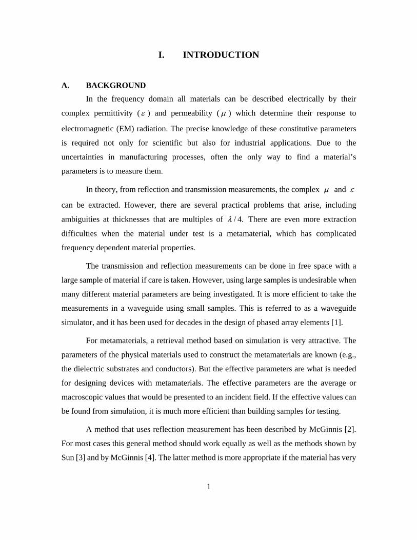
A. BACKGROUND In the frequency domain all materials can be described electrically by their
complex permittivity ( ε ) and permeability ( µ ) which determine their response to
electromagnetic (EM) radiation. The precise knowledge of these constitutive parameters
is required not only for scientific but also for industrial applications. Due to the
uncertainties in manufacturing processes, often the only way to find a material’s
parameters is to measure them.
In theory, from reflection and transmission measurements, the complex µ and ε
can be extracted. However, there are several practical problems that arise, including
ambiguities at thicknesses that are multiples of / 4.λ There are even more extraction
difficulties when the material under test is a metamaterial, which has complicated
frequency dependent material properties.
The transmission and reflection measurements can be done in free space with a
large sample of material if care is taken. However, using large samples is undesirable when
many different material parameters are being investigated. It is more efficient to take the
measurements in a waveguide using small samples. This is referred to as a waveguide
simulator, and it has been used for decades in the design of phased array elements [1].
For metamaterials, a retrieval method based on simulation is very attractive. The
parameters of the physical materials used to construct the metamaterials are known (e.g.,
the dielectric substrates and conductors). But the effective parameters are what is needed
for designing devices with metamaterials. The effective parameters are the average or
macroscopic values that would be presented to an incident field. If the effective values can
be found from simulation, it is much more efficient than building samples for testing.
A method that uses reflection measurement has been described by McGinnis [2].
For most cases this general method should work equally as well as the methods shown by
Sun [3] and by McGinnis [4]. The latter method is more appropriate if the material has very
2
high permittivity, permeability or attenuation, or the measurement varies from sample to
sample. A newer method [5] using the same concept as [4] but with slightly different
formulas, was used in this thesis.
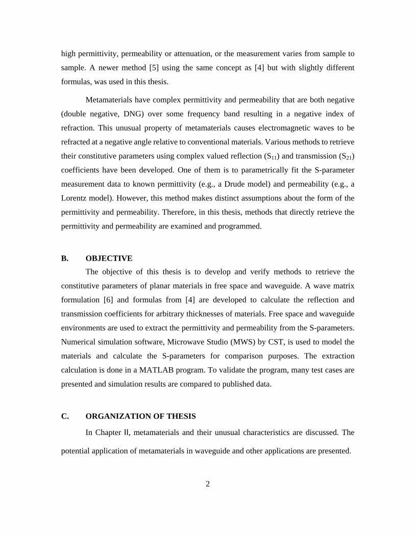
Metamaterials have complex permittivity and permeability that are both negative
(double negative, DNG) over some frequency band resulting in a negative index of
refraction. This unusual property of metamaterials causes electromagnetic waves to be
refracted at a negative angle relative to conventional materials. Various methods to retrieve
their constitutive parameters using complex valued reflection (S11) and transmission (S21)
coefficients have been developed. One of them is to parametrically fit the S-parameter
measurement data to known permittivity (e.g., a Drude model) and permeability (e.g., a
Lorentz model). However, this method makes distinct assumptions about the form of the
permittivity and permeability. Therefore, in this thesis, methods that directly retrieve the
permittivity and permeability are examined and programmed.
B. OBJECTIVE The objective of this thesis is to develop and verify methods to retrieve the
constitutive parameters of planar materials in free space and waveguide. A wave matrix
formulation [6] and formulas from [4] are developed to calculate the reflection and
transmission coefficients for arbitrary thicknesses of materials. Free space and waveguide
environments are used to extract the permittivity and permeability from the S-parameters.
Numerical simulation software, Microwave Studio (MWS) by CST, is used to model the
materials and calculate the S-parameters for comparison purposes. The extraction
calculation is done in a MATLAB program. To validate the program, many test cases are
presented and simulation results are compared to published data.
C. ORGANIZATION OF THESIS
In Chapter Ⅱ, metamaterials and their unusual characteristics are discussed. The
potential application of metamaterials in waveguide and other applications are presented.
3
In Chapter Ⅲ, the free space environment retrieval method is proposed and
discussed. The simulation set up using MWS for the free space environment is presented.
The results extracted from the S-parameters are compared with published data.
In Chapter Ⅳ, the waveguide environment simulation set up and retrieval methods
are presented. The extracted permittivity and permeability are described and compared.
Finally in Chapter Ⅴ, the results, conclusions and suggestions for future studies are
discussed.

4
THIS PAGE INTENTIONALLY LEFT BLANK
5
II. METAMATERIALS
A. INTRODUCTION Metamaterials, also called left-handed materials (LHMs), are a class of composite
materials artificially built to exhibit unusual properties not found in nature. The history of
LHMs can be tracked back to Veselago’s theoretical hypothesis in 1968 [7], in which he
demonstrated that the LHMs would result in unusual optical phenomena when light passed
through them. In 2000, the UCSD (University of California, San Diego) group, which was
following the work by Pendry et al. [8-10], demonstrated the first left-handed material [11,
12]. This LHM made use of an array of conducting, nonmagnetic elements and an array of
conducting continuous wires to achieve a negative effective permittivity and negative
effective permeability respectively.
B. NEGATIVE PERMITTIVITY AND PERMEABILITY
In general, for a passive medium, assuming a j te ω time dependence,
( )0 0r r rjε ε ε ε ε ε= = −' " (2.1)
and
( )0 0r r rjµ µ µ µ µ µ= = −' " (2.2)
where 120 8.85 10 F/mε −= × and 7
0 4 10 H/m.µ π −= × For most materials µ and ε are
scalars, however, for anisotropic materials, matrices must be used:
[ ]D Eε= (2.3)
and
[ ]B Hµ= (2.4)
where, for example
[ ] 0
xx xy xz
yx yy yz
zx zy zz
ε ε εε ε ε ε ε
ε ε ε
⎛ ⎞⎜ ⎟
= ⎜ ⎟⎜ ⎟⎝ ⎠
(2.5)

6
The elements ijε ( , ,i j x y= or z ) are the complex relative values that completely
describe the permittivity of the material. A similar matrix can be defined for the
permeability:
[ ] 0
xx xy xz
yx yy yz
zx zy zz
µ µ µµ µ µ µ µ
µ µ µ
⎛ ⎞⎜ ⎟
= ⎜ ⎟⎜ ⎟⎝ ⎠
(2.6)
Metamaterials are artificial materials that are designed to have unique
electromagnetic properties such as a negative index of refraction. For a DNG metamaterial,
one should write the permittivity and permeability as [13]:
r r rjε ε ε= − = (2.7)
and
r r rjµ µ µ= − = (2.8)
The wavenumber and the wave impedance can be described as follows:
0 0 0 0r r r rk ω ε ε µ µ ω ε ε µ µ= = − (2.9)
and
0 0rr
r r
µµη η η
ε ε= = (2.10)
The index of refraction for a DNG material can be obtained from the formula:
r r r rn ε µ ε µ= = − (2.11)
The different combinations of real permeability and permittivity with various signs
are listed in Table 1.

7
n 0rε > 0rε <
0rµ > + j
0rµ < j -
Table 1. Sign of Index of Refraction
For a DNG material the negative sign flips the angle of refraction in Snell’s law.
For example, a negative angle of refraction equal and opposite to the standard angle of
incidence can be clearly observed in Figure 1.
DNG
Free Space
Free Space
Figure 1. Electric Field Intensity Distribution for the Wave Interaction with a DNG
Metamaterial (After Ref. [13])
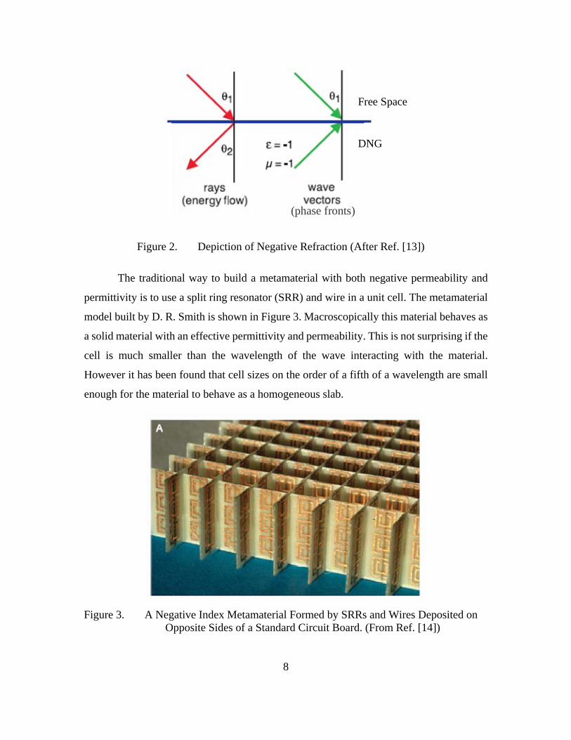
As can be seen in Figure 2, on the left, a ray enters a negatively refracting medium
and is bent the opposite way relative to the surface normal compared to a conventional
right handed material. On the right is the wave vector. Negative refraction requires that the
wave vector (direction of phase fronts) and Poynting vector (direction of energy flow)
point in opposite directions [13].
8
Free Space
DNG
(phase fronts)
Figure 2. Depiction of Negative Refraction (After Ref. [13])
The traditional way to build a metamaterial with both negative permeability and
permittivity is to use a split ring resonator (SRR) and wire in a unit cell. The metamaterial
model built by D. R. Smith is shown in Figure 3. Macroscopically this material behaves as
a solid material with an effective permittivity and permeability. This is not surprising if the
cell is much smaller than the wavelength of the wave interacting with the material.
However it has been found that cell sizes on the order of a fifth of a wavelength are small
enough for the material to behave as a homogeneous slab.
Figure 3. A Negative Index Metamaterial Formed by SRRs and Wires Deposited on
Opposite Sides of a Standard Circuit Board. (From Ref. [14])
9
There are also new concepts for DNG metamaterials. In Chapter III and Chapter
IV, these “new” metamaterials were investigated, one of which uses short wire pairs while
the other uses H-type pairs as inclusions. The major difference between “traditional” and
“new” metamaterials is that “new” metamaterials are relatively easy to fabricate, which
make them easier to use and may hasten their development.
C. APPLICATIONS OF METAMATERIALS Metamaterials have attracted a lot of attention in recent years. Some of the possible
applications of metamaterials are discussed below.
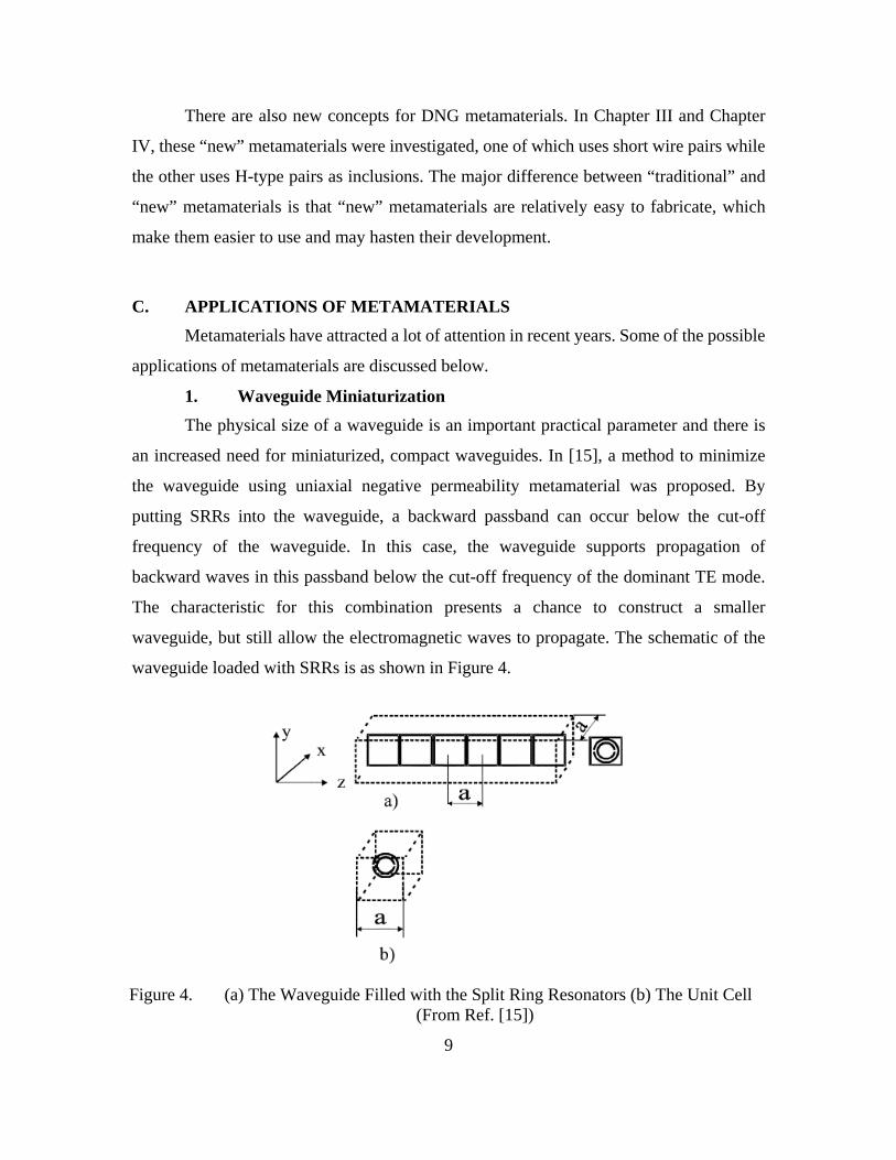
1. Waveguide Miniaturization
The physical size of a waveguide is an important practical parameter and there is
an increased need for miniaturized, compact waveguides. In [15], a method to minimize
the waveguide using uniaxial negative permeability metamaterial was proposed. By
putting SRRs into the waveguide, a backward passband can occur below the cut-off
frequency of the waveguide. In this case, the waveguide supports propagation of
backward waves in this passband below the cut-off frequency of the dominant TE mode.
The characteristic for this combination presents a chance to construct a smaller
waveguide, but still allow the electromagnetic waves to propagate. The schematic of the
waveguide loaded with SRRs is as shown in Figure 4.
Figure 4. (a) The Waveguide Filled with the Split Ring Resonators (b) The Unit Cell
(From Ref. [15])

10
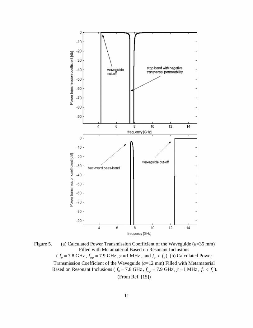
The difference between the waveguides loaded with SRRs with the resonant
frequency of SRRs above the cut-off frequency cf and below cf ( 12.5 GHzcf = for
12 mma = , 4.28 GHzcf = for 35a = mm) is described in Figure 5. Note that when
the resonant frequency of SRRs ( )0f is higher than the cut-off frequency of the
waveguide, a stop band with negative transversal permeability is observed. On the other
hand, when 0 cf f< , a backward passband is observed below the cut-off frequency of the
waveguide.
11
Figure 5. (a) Calculated Power Transmission Coefficient of the Waveguide (a=35 mm)
Filled with Metamaterial Based on Resonant Inclusions ( 0 7.8 GHzf = , 7.9 GHzmpf = , 1 MHzγ = , and 0 cf f> ). (b) Calculated Power
Transmission Coefficient of the Waveguide (a=12 mm) Filled with Metamaterial Based on Resonant Inclusions ( 0 7.8 GHzf = , 7.9 GHzmpf = , 1 MHzγ = , 0 cf f< ).
(From Ref. [15])
12
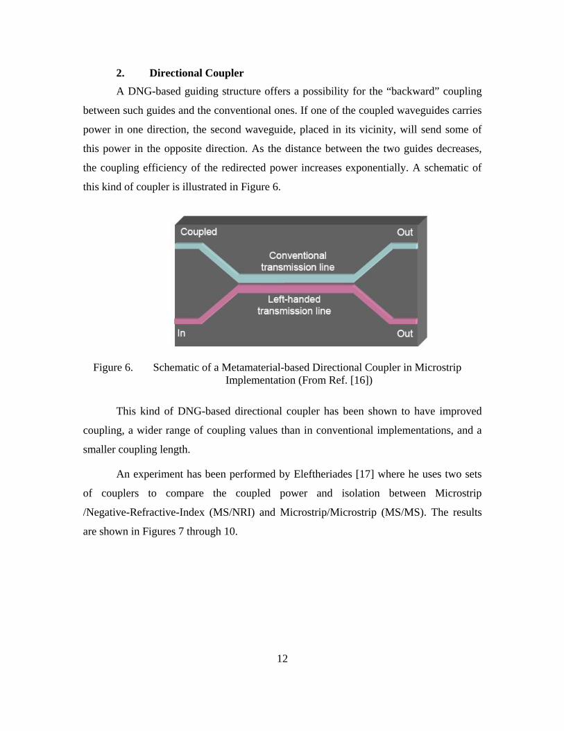
2. Directional Coupler
A DNG-based guiding structure offers a possibility for the “backward” coupling
between such guides and the conventional ones. If one of the coupled waveguides carries
power in one direction, the second waveguide, placed in its vicinity, will send some of
this power in the opposite direction. As the distance between the two guides decreases,
the coupling efficiency of the redirected power increases exponentially. A schematic of
this kind of coupler is illustrated in Figure 6.
Figure 6. Schematic of a Metamaterial-based Directional Coupler in Microstrip
Implementation (From Ref. [16])
This kind of DNG-based directional coupler has been shown to have improved
coupling, a wider range of coupling values than in conventional implementations, and a
smaller coupling length.
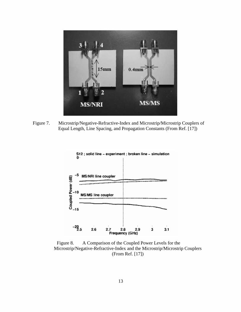
An experiment has been performed by Eleftheriades [17] where he uses two sets
of couplers to compare the coupled power and isolation between Microstrip
/Negative-Refractive-Index (MS/NRI) and Microstrip/Microstrip (MS/MS). The results
are shown in Figures 7 through 10.
13
Figure 7. Microstrip/Negative-Refractive-Index and Microstrip/Microstrip Couplers of
Equal Length, Line Spacing, and Propagation Constants (From Ref. [17])
Figure 8. A Comparison of the Coupled Power Levels for the
Microstrip/Negative-Refractive-Index and the Microstrip/Microstrip Couplers (From Ref. [17])
14
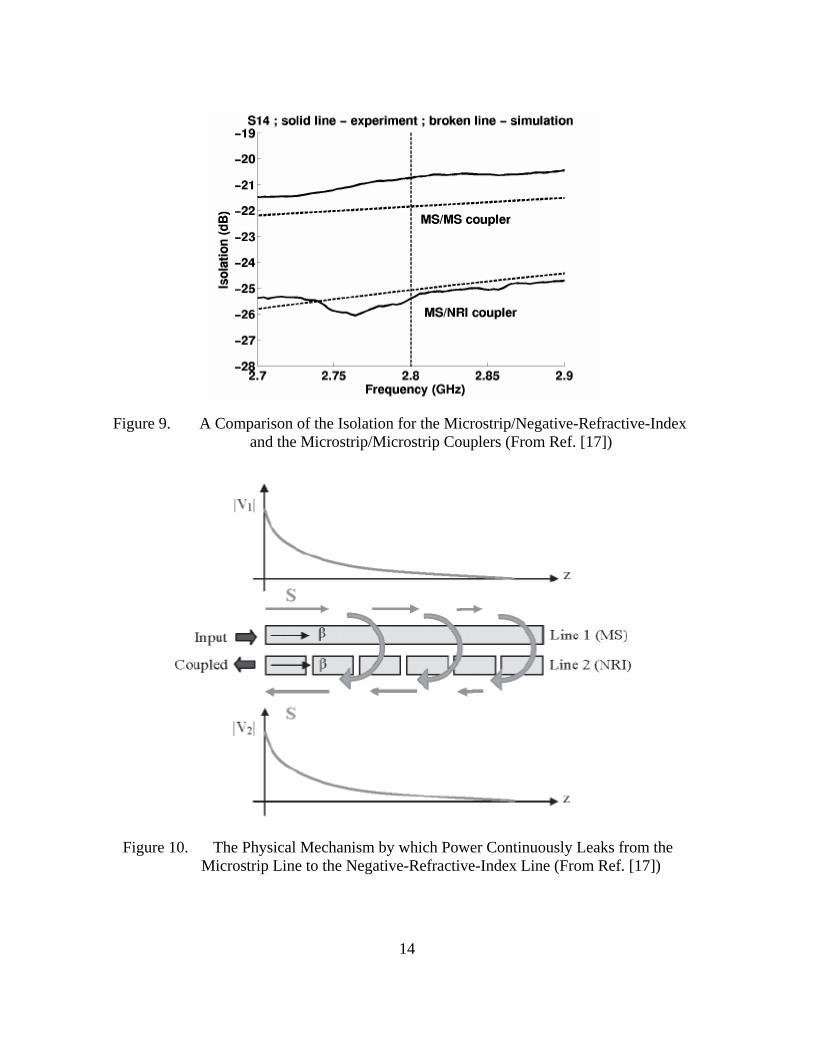
Figure 9. A Comparison of the Isolation for the Microstrip/Negative-Refractive-Index
and the Microstrip/Microstrip Couplers (From Ref. [17])
Figure 10. The Physical Mechanism by which Power Continuously Leaks from the
Microstrip Line to the Negative-Refractive-Index Line (From Ref. [17])

15
For MS/NRI, the coupled power is 6 dB higher than that in MS/MS (Figure 7) and
the isolation for MS/NRI is about 4 dB lower than that in the MS/MS structure (Figure 8).
The new MS/NRI coupler exhibits better performance than the traditional MS/MS
coupler in terms of higher coupling power, isolation, and lower return loss. The coupling
mechanism is depicted in Figure 10.
There are more applications that can exploit the unique characteristics of
metamaterials, such as [16]:
1. Wideband directive antennas
2. Perfect lens and superlens
3. Phase compensators and sub-wavelength resonators
4. Guided wave applications
5. Electrically small antennas
6. Filtering and beam shaping
The two examples and the list above include only a few from a wide variety of
applications. As more and more people become aware of these new materials and their
properties, one can expect to see more applications using metamaterials. In the next
chapter the extraction of µ and ε for bulk materials in free space is discussed. The
procedure is applied to both conventional materials and metamaterials.

16
THIS PAGE INTENTIONALLY LEFT BLANK
17
III. FREE SPACE ENVIRONMENT
A. INTRODUCTION In this chapter, measurements on materials in the free space environment are used
to extract the constitutive parameters from scattering parameters. In order to verify the
accuracy of scattering parameters generated from simulation using MWS, the wave matrix
approach [18] is used to calculate the reflection and transmission coefficients and compare
with those generated from simulation.
B. FORMULATION
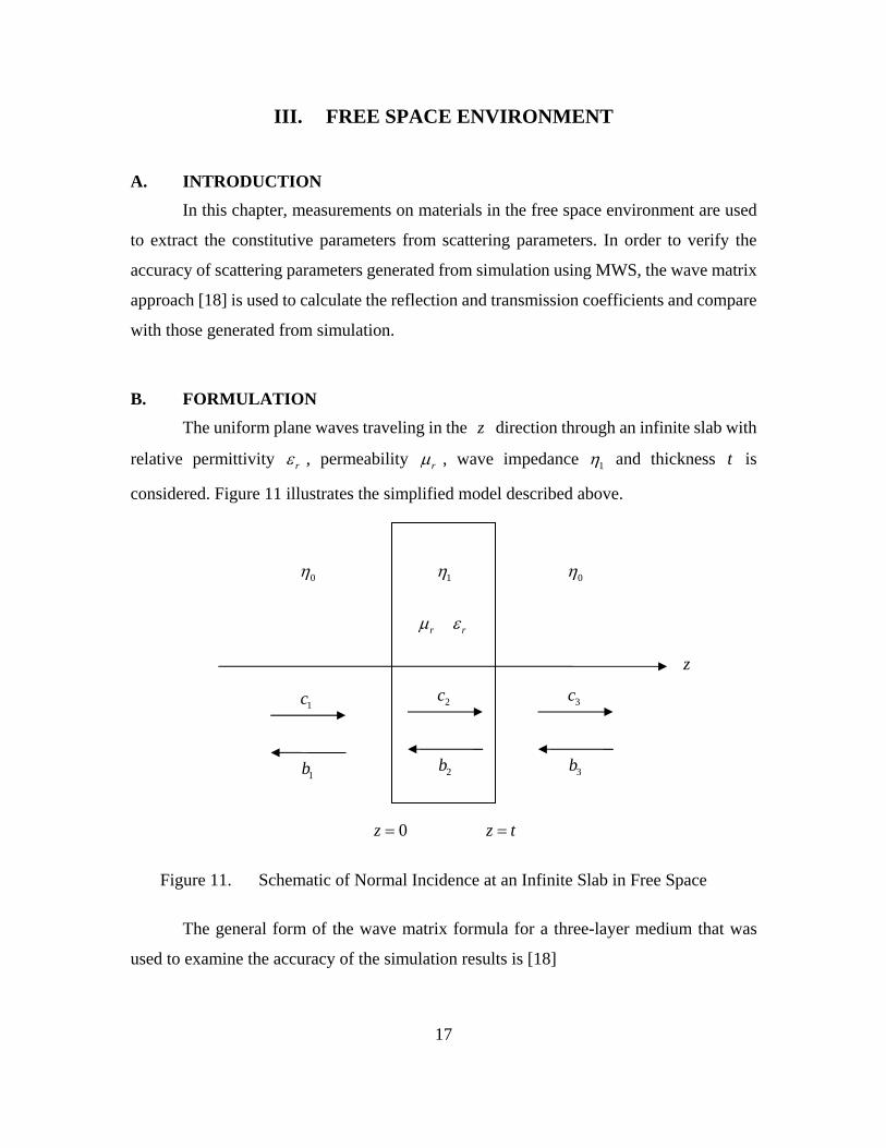
The uniform plane waves traveling in the z direction through an infinite slab with
relative permittivity rε , permeability rµ , wave impedance 1η and thickness t is
considered. Figure 11 illustrates the simplified model described above.
Figure 11. Schematic of Normal Incidence at an Infinite Slab in Free Space
The general form of the wave matrix formula for a three-layer medium that was
used to examine the accuracy of the simulation results is [18]
0z = z t=
z
0η 0η1η
1b
rµ rε
2b 3b
1c 2c 3c

18
2
3 31 11 12
1 21 221 3 3
1 n n
n n
j jn
j jn n n
c cc a ae R ea ab b bT R e e
φ φ
φ φ
−
−=
⎛ ⎞ ⎡ ⎤ ⎡ ⎤⎡ ⎤ ⎛ ⎞= ≡⎜ ⎟ ⎜ ⎟⎢ ⎥ ⎢ ⎥⎢ ⎥
⎝ ⎠⎣ ⎦ ⎣ ⎦ ⎣ ⎦⎝ ⎠∏ (3.1)
If the thickness of the third layer extends to ∞ , then it is possible to state that 3 0b = . The
total transmission and reflection coefficients of the slab become
3
1 11
1cTc a
= = (3.2)
and
1 21
1 11
b aRc a
= = (3.3)
The difference between the calculated and simulated transmission and reflection
coefficients for a normal material (both selected µ and ε are positive) are presented in
the next section.
The retrieval method used in the first part of this thesis is based on the approach
used by Xudong Chen et al in [19], where the S-parameters are defined in terms of the
reflection and transmission coefficients as
11S R= (3.4)
and
021
jk dS Te= (3.5)
where 0k is the wave number in free space and d is the thickness of the material being
examined. The impedance Z and the refractive index n are
( )( )
2 211 21
2 211 21
11
S SZ
S S+ −
= ±− −
(3.6)
and
( ) ( ){ }0 0
0
1 Im ln 2 Re lnink d ink dn e m j ek d
π⎡ ⎤ ⎡ ⎤⎡ ⎤ ⎡ ⎤= + −⎣ ⎦ ⎣ ⎦⎣ ⎦ ⎣ ⎦ (3.7)
19
where m is an integer related to the branch index of the real part of n and the value of 0jnk de is obtained from 11S , 21S , and z from
0 21
11111
jnk d Se ZSZ
=−
−+
(3.8)
As described in [19], Z and n are related so that their relationship can be used to
determine the correct sign of Z . Two cases are distinguished in order to correctly find the
sign of Z . The first case is for Re( )Z δ≥ , where δ is a positive number and for which
Re( ) 0Z ≥ . In the second case, the sign of Z is chosen so that the corresponding
Im( ) 0n ≥ , or equivalently 0 1jnk de ≤ . The method to precisely determine the branch of
Re( )n can be found in [19].
C. RETRIEVAL USING NUMERICALLY GENERATED S-PARAMETER
In the first part of this section, it is demonstrated that the simulated data is accurate
by comparing it with the data calculated from the wave matrix formula. The effectiveness
of the retrieval program is also examined by extracting the constitutive parameters of the
model and comparing them with the original values used to compute T and R, and
published paper data.
Simulations were done with CST Microwave Studio (Computer Simulation
Technology GmbH, Darmstadt, Germany), which uses the finite-integration method in the
time domain to determine reflection and/or transmission properties of any given structures.
1. Model 1 - Normal Material
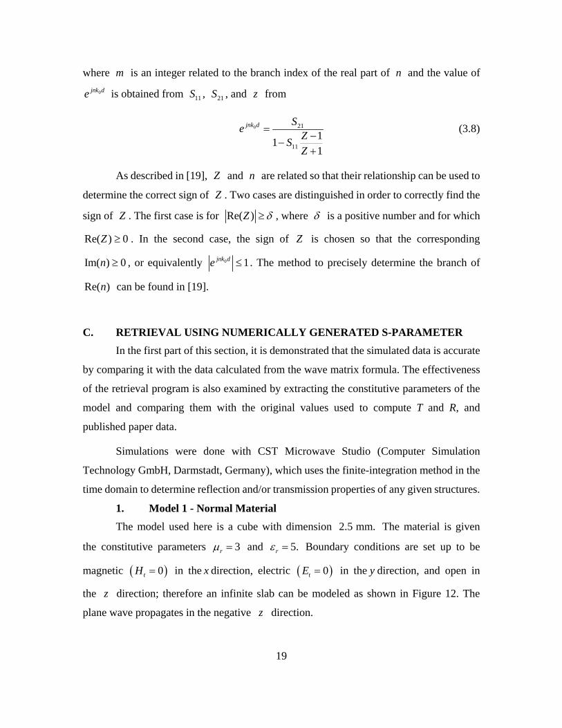
The model used here is a cube with dimension 2.5 mm. The material is given
the constitutive parameters 3rµ = and 5.rε = Boundary conditions are set up to be
magnetic ( )0tH = in the x direction, electric ( )0tE = in the y direction, and open in
the z direction; therefore an infinite slab can be modeled as shown in Figure 12. The
plane wave propagates in the negative z direction.
20
Figure 12. Normal Material with 3rµ = and 5rε = , and 2.5 mm side length
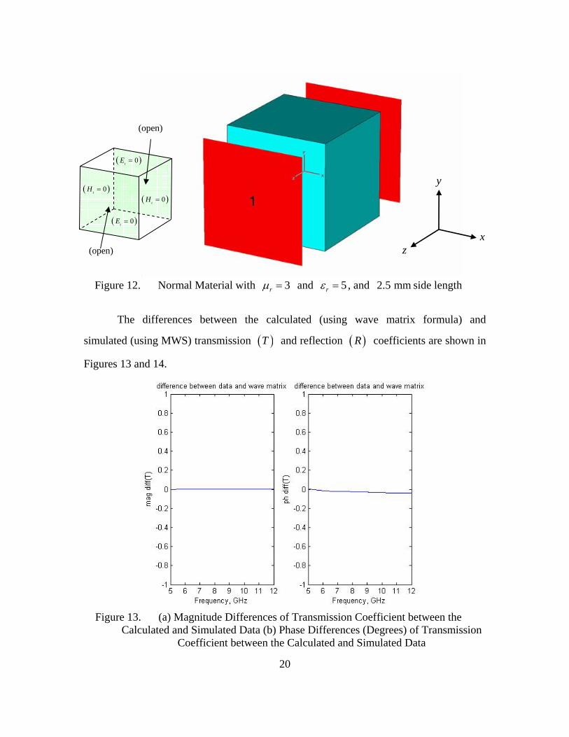
The differences between the calculated (using wave matrix formula) and
simulated (using MWS) transmission ( )T and reflection ( )R coefficients are shown in
Figures 13 and 14.
Figure 13. (a) Magnitude Differences of Transmission Coefficient between the
Calculated and Simulated Data (b) Phase Differences (Degrees) of Transmission Coefficient between the Calculated and Simulated Data
z
y
x
( )0tH = ( )0tH =
( )0tE =
( )0tE =
(open)
(open)
21
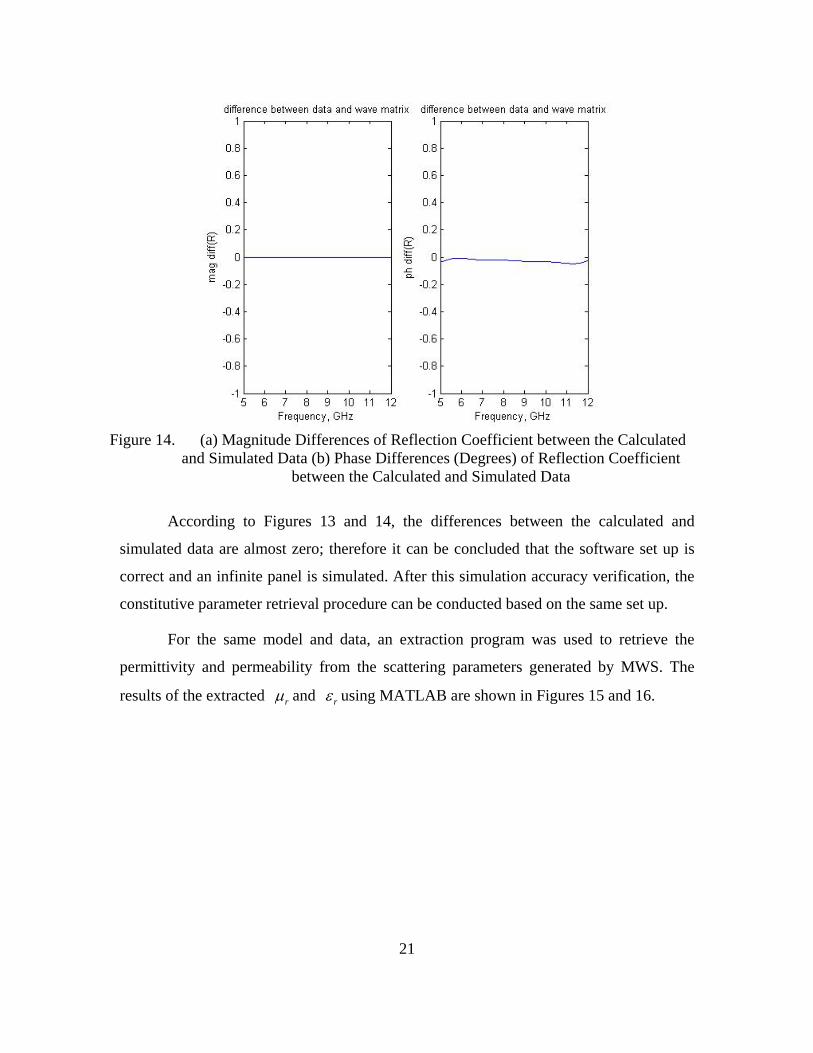
Figure 14. (a) Magnitude Differences of Reflection Coefficient between the Calculated
and Simulated Data (b) Phase Differences (Degrees) of Reflection Coefficient between the Calculated and Simulated Data
According to Figures 13 and 14, the differences between the calculated and
simulated data are almost zero; therefore it can be concluded that the software set up is
correct and an infinite panel is simulated. After this simulation accuracy verification, the
constitutive parameter retrieval procedure can be conducted based on the same set up.
For the same model and data, an extraction program was used to retrieve the
permittivity and permeability from the scattering parameters generated by MWS. The
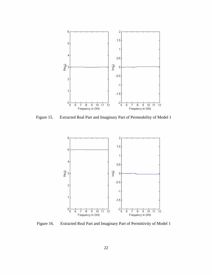
results of the extracted rµ and rε using MATLAB are shown in Figures 15 and 16.
22
Figure 15. Extracted Real Part and Imaginary Part of Permeability of Model 1
Figure 16. Extracted Real Part and Imaginary Part of Permittivity of Model 1
23
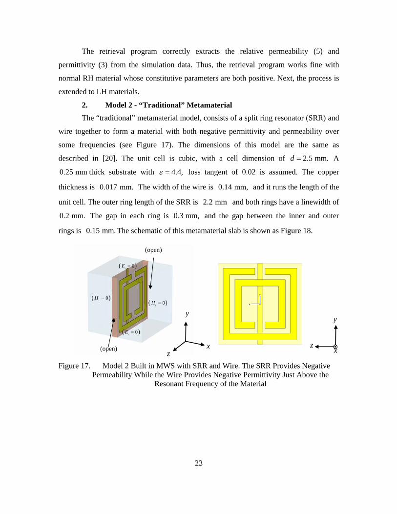
The retrieval program correctly extracts the relative permeability (5) and
permittivity (3) from the simulation data. Thus, the retrieval program works fine with
normal RH material whose constitutive parameters are both positive. Next, the process is
extended to LH materials.
2. Model 2 - “Traditional” Metamaterial The “traditional” metamaterial model, consists of a split ring resonator (SRR) and
wire together to form a material with both negative permittivity and permeability over
some frequencies (see Figure 17). The dimensions of this model are the same as
described in [20]. The unit cell is cubic, with a cell dimension of 2.5 mm.d = A
0.25 mm thick substrate with 4.4,ε = loss tangent of 0.02 is assumed. The copper
thickness is 0.017 mm. The width of the wire is 0.14 mm, and it runs the length of the
unit cell. The outer ring length of the SRR is 2.2 mm and both rings have a linewidth of
0.2 mm. The gap in each ring is 0.3 mm, and the gap between the inner and outer
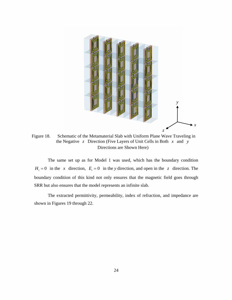
rings is 0.15 mm. The schematic of this metamaterial slab is shown as Figure 18.
Figure 17. Model 2 Built in MWS with SRR and Wire. The SRR Provides Negative
Permeability While the Wire Provides Negative Permittivity Just Above the Resonant Frequency of the Material
z
y
x z
y
x
( )0tH = ( )0tH =
( )0tE =
( )0tE =
(open)
(open)
24
Figure 18. Schematic of the Metamaterial Slab with Uniform Plane Wave Traveling in
the Negative z Direction (Five Layers of Unit Cells in Both x and y Directions are Shown Here)
The same set up as for Model 1 was used, which has the boundary condition
0tH = in the x direction, 0tE = in the y direction, and open in the z direction. The
boundary condition of this kind not only ensures that the magnetic field goes through
SRR but also ensures that the model represents an infinite slab.
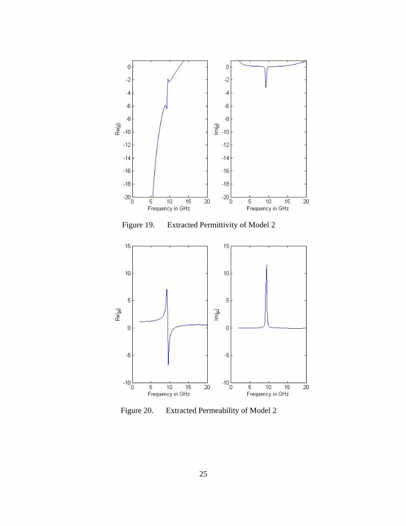
The extracted permittivity, permeability, index of refraction, and impedance are
shown in Figures 19 through 22.
z
y
x
25
Figure 19. Extracted Permittivity of Model 2
Figure 20. Extracted Permeability of Model 2
26
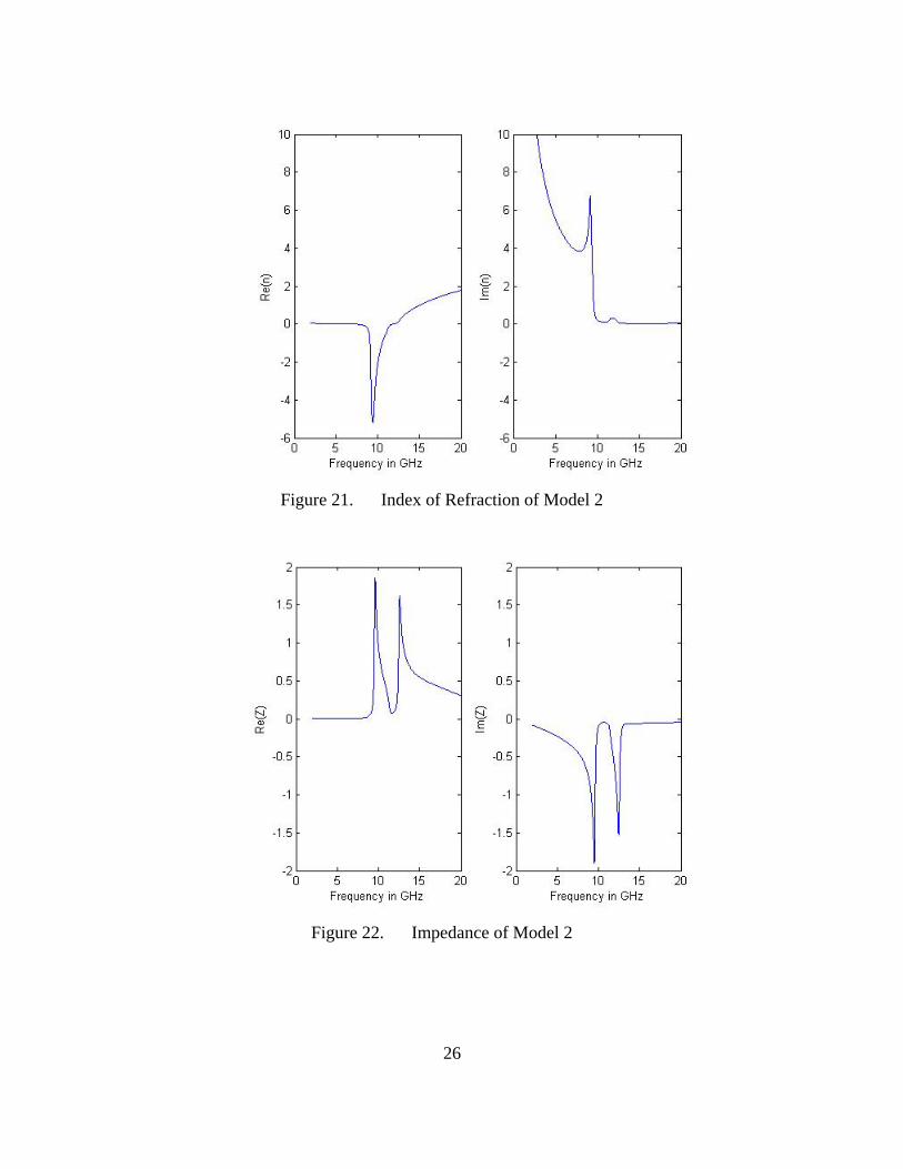
Figure 21. Index of Refraction of Model 2
Figure 22. Impedance of Model 2
27
The extracted constitutive parameters, index of refraction, and impedance of the
material are very close to the published data [20]. However, in the simulation process, it
was found that the meshing property is very important in terms of the accuracy of the
scattering parameters and the position of the resonant frequency. Because the author does
not have the exact meshing parameters which the published paper used, the final results
are not identical to the published data, although they are very close.
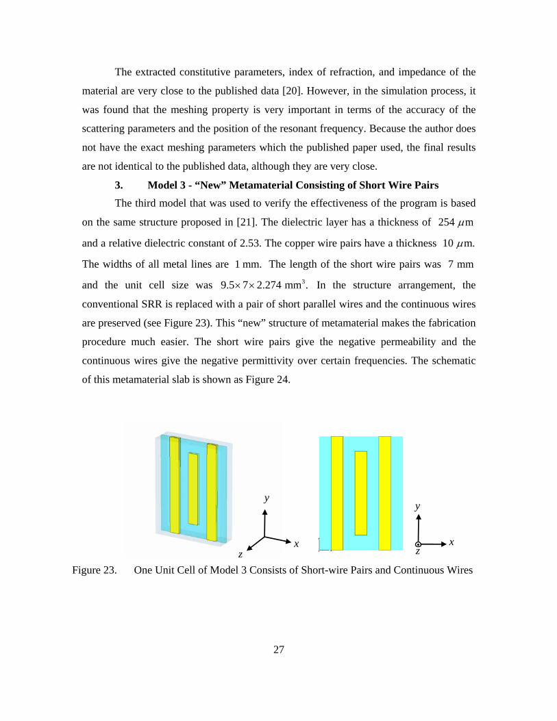
3. Model 3 - “New” Metamaterial Consisting of Short Wire Pairs The third model that was used to verify the effectiveness of the program is based
on the same structure proposed in [21]. The dielectric layer has a thickness of 254 mµ
and a relative dielectric constant of 2.53. The copper wire pairs have a thickness 10 m.µ
The widths of all metal lines are 1 mm. The length of the short wire pairs was 7 mm
and the unit cell size was 39.5 7 2.274 mm .× × In the structure arrangement, the
conventional SRR is replaced with a pair of short parallel wires and the continuous wires
are preserved (see Figure 23). This “new” structure of metamaterial makes the fabrication
procedure much easier. The short wire pairs give the negative permeability and the
continuous wires give the negative permittivity over certain frequencies. The schematic
of this metamaterial slab is shown as Figure 24.
Figure 23. One Unit Cell of Model 3 Consists of Short-wire Pairs and Continuous Wires
z
y
x z
y
x
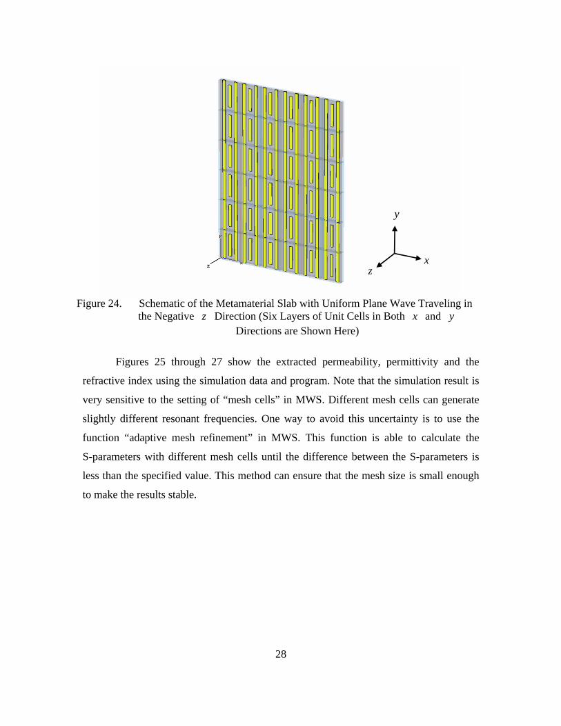
28
Figure 24. Schematic of the Metamaterial Slab with Uniform Plane Wave Traveling in
the Negative z Direction (Six Layers of Unit Cells in Both x and y Directions are Shown Here)
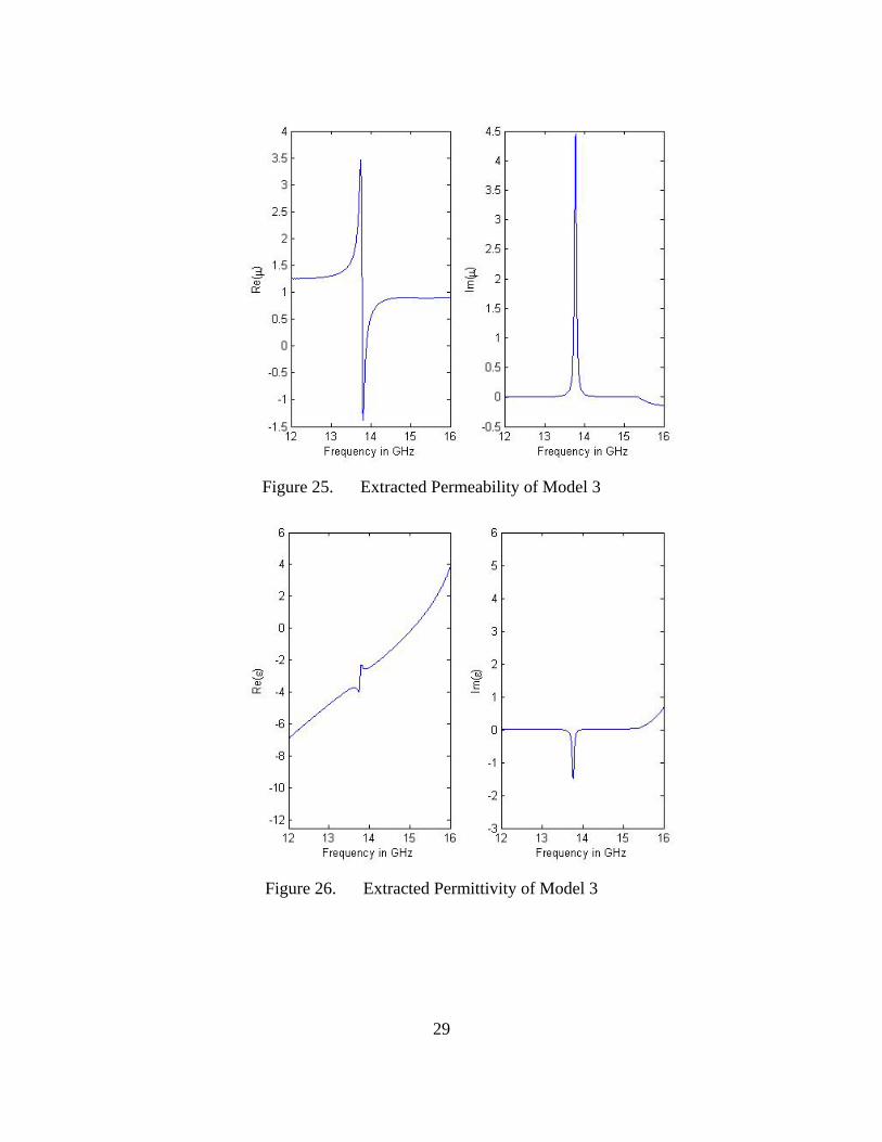
Figures 25 through 27 show the extracted permeability, permittivity and the
refractive index using the simulation data and program. Note that the simulation result is
very sensitive to the setting of “mesh cells” in MWS. Different mesh cells can generate
slightly different resonant frequencies. One way to avoid this uncertainty is to use the
function “adaptive mesh refinement” in MWS. This function is able to calculate the
S-parameters with different mesh cells until the difference between the S-parameters is
less than the specified value. This method can ensure that the mesh size is small enough
to make the results stable.
z
y
x
29
Figure 25. Extracted Permeability of Model 3
Figure 26. Extracted Permittivity of Model 3
30
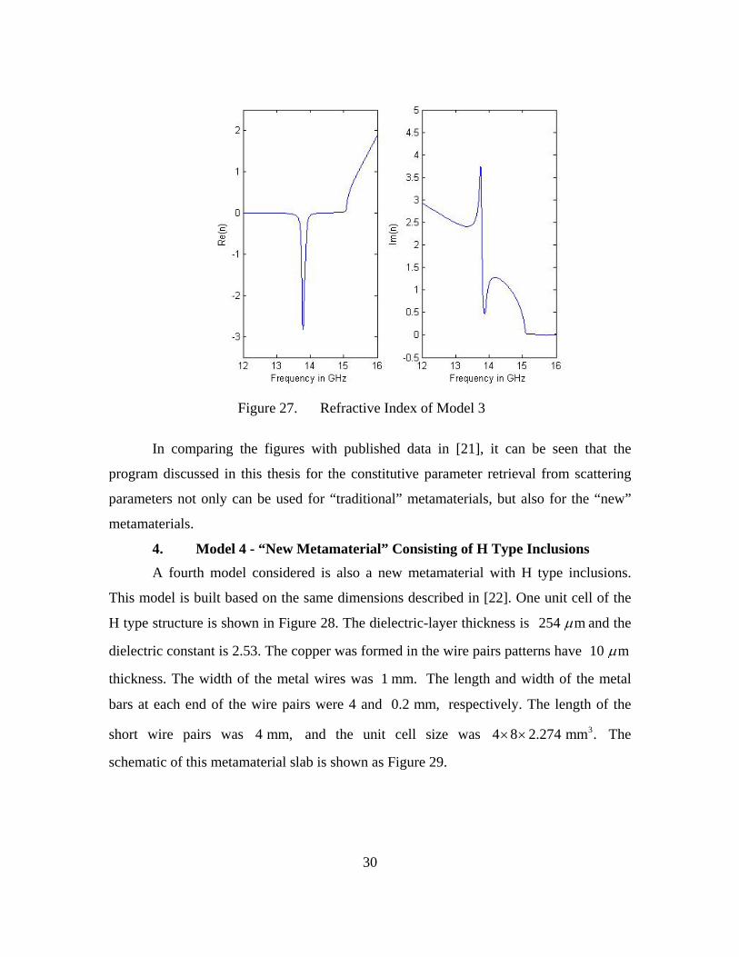
Figure 27. Refractive Index of Model 3
In comparing the figures with published data in [21], it can be seen that the
program discussed in this thesis for the constitutive parameter retrieval from scattering
parameters not only can be used for “traditional” metamaterials, but also for the “new”
metamaterials.
4. Model 4 - “New Metamaterial” Consisting of H Type Inclusions A fourth model considered is also a new metamaterial with H type inclusions.
This model is built based on the same dimensions described in [22]. One unit cell of the
H type structure is shown in Figure 28. The dielectric-layer thickness is 254 mµ and the
dielectric constant is 2.53. The copper was formed in the wire pairs patterns have 10 mµ
thickness. The width of the metal wires was 1 mm. The length and width of the metal
bars at each end of the wire pairs were 4 and 0.2 mm, respectively. The length of the
short wire pairs was 4 mm, and the unit cell size was 34 8 2.274 mm .× × The
schematic of this metamaterial slab is shown as Figure 29.
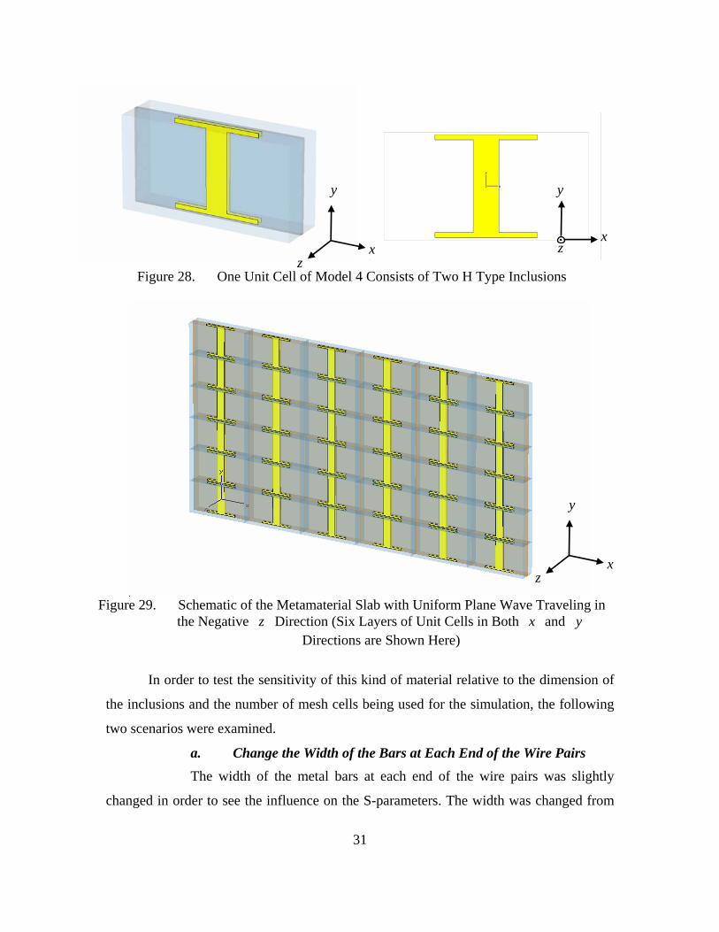
31
Figure 28. One Unit Cell of Model 4 Consists of Two H Type Inclusions
Figure 29. Schematic of the Metamaterial Slab with Uniform Plane Wave Traveling in
the Negative z Direction (Six Layers of Unit Cells in Both x and y Directions are Shown Here)
In order to test the sensitivity of this kind of material relative to the dimension of
the inclusions and the number of mesh cells being used for the simulation, the following
two scenarios were examined.
a. Change the Width of the Bars at Each End of the Wire Pairs
The width of the metal bars at each end of the wire pairs was slightly
changed in order to see the influence on the S-parameters. The width was changed from
z
y
x z
y
x
z
y
x

32
0.2 mm to 0.25 mm and the adaptive mesh refinement function was enabled so as to
obtain optimal results. The S-parameters for the original 0.2 mm and the modified 0.25
mm structures are presented in Figures 30 and 31.
Figure 30. Magnitude of 21S of the Original 0.2 mm Model
Figure 31. Magnitude of 21S of the Modified 0.25 mm Model
The resonant frequency in Figure 30 with the optimized 21S value occurs
around 15.65 GHz (purple curve). The optimized resonant frequency in Figure 31 (width
33
changed by 0.05 mm) shifted to the left to around 15.25 GHz (purple curve). This
observation shows that the resonant frequency is very sensitive to the dimension of the
inclusions.
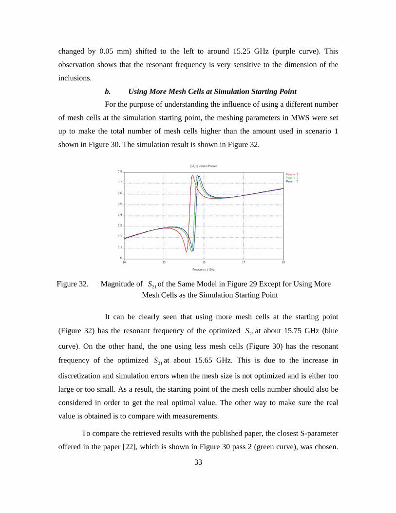
b. Using More Mesh Cells at Simulation Starting Point For the purpose of understanding the influence of using a different number
of mesh cells at the simulation starting point, the meshing parameters in MWS were set
up to make the total number of mesh cells higher than the amount used in scenario 1
shown in Figure 30. The simulation result is shown in Figure 32.
Figure 32. Magnitude of 21S of the Same Model in Figure 29 Except for Using More
Mesh Cells as the Simulation Starting Point
It can be clearly seen that using more mesh cells at the starting point
(Figure 32) has the resonant frequency of the optimized 21S at about 15.75 GHz (blue
curve). On the other hand, the one using less mesh cells (Figure 30) has the resonant
frequency of the optimized 21S at about 15.65 GHz. This is due to the increase in
discretization and simulation errors when the mesh size is not optimized and is either too
large or too small. As a result, the starting point of the mesh cells number should also be
considered in order to get the real optimal value. The other way to make sure the real
value is obtained is to compare with measurements.
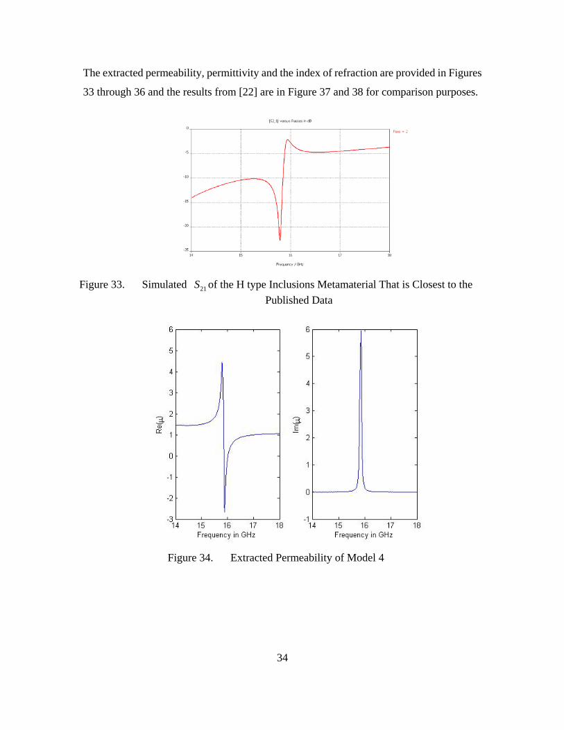
To compare the retrieved results with the published paper, the closest S-parameter
offered in the paper [22], which is shown in Figure 30 pass 2 (green curve), was chosen.
34
The extracted permeability, permittivity and the index of refraction are provided in Figures
33 through 36 and the results from [22] are in Figure 37 and 38 for comparison purposes.
Figure 33. Simulated 21S of the H type Inclusions Metamaterial That is Closest to the
Published Data
Figure 34. Extracted Permeability of Model 4
35
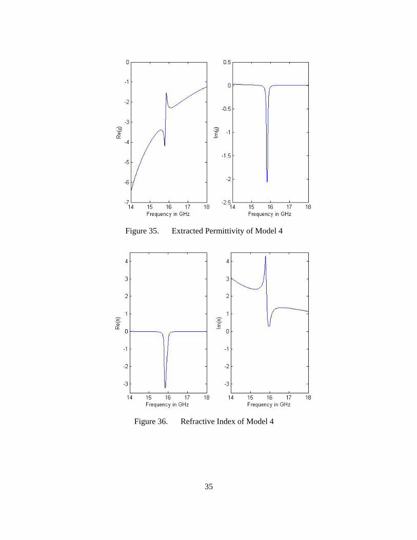
Figure 35. Extracted Permittivity of Model 4
Figure 36. Refractive Index of Model 4
36
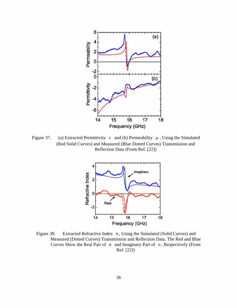
Figure 37. (a) Extracted Permittivity ε and (b) Permeability µ , Using the Simulated
(Red Solid Curves) and Measured (Blue Dotted Curves) Transmission and Reflection Data (From Ref. [22])
Figure 38. Extracted Refractive Index n , Using the Simulated (Solid Curves) and
Measured (Dotted Curves) Transmission and Reflection Data. The Red and Blue Curves Show the Real Part of n and Imaginary Part of n , Respectively (From
Ref. [22])
37
The extracted constitutive parameters and the refractive index are very close to the
published data. Again the discrepancy is caused by the simulation set up which is very
sensitive to the dimension of inclusions and the number of mesh cells used.
D. SUMMARY In this chapter, four models were used to extract the permeability and permittivity
from the simulated S-parameters. The formula used was based on the free space
environment; therefore boundary conditions had to be defined so that the model could be
treated as an infinite slab. Test cases were performed to verify the effectiveness of the
simulation set up. It was found that the differences between the simulated and calculated
S-parameters were negligible. The resonant frequencies of metamaterial models were very
sensitive to both the dimensions and mesh cell number; therefore, it is good to have both
simulation and measurement data for comparison purposes. The above models have shown
that the extraction program discussed in this thesis can work not only for normal materials
but also metamaterials.

38
THIS PAGE INTENTIONALLY LEFT BLANK
39
IV. WAVEGUIDE ENVIRONMENT
A. INTRODUCTION In this chapter, a retrieval method for materials in a waveguide environment is used
to extract the constitutive parameters of the materials. The purpose of this waveguide
method is to demonstrate that the method of images can be applied to structures for
permeability and permittivity retrieval. Therefore a small sample of material is enough to
perform the extraction or measurement procedure. The results from the free space
environment method are also compared to support this hypothesis.
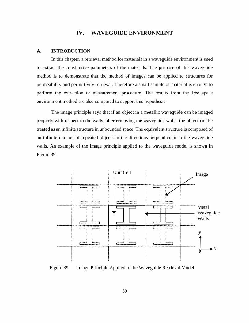
The image principle says that if an object in a metallic waveguide can be imaged
properly with respect to the walls, after removing the waveguide walls, the object can be
treated as an infinite structure in unbounded space. The equivalent structure is composed of
an infinite number of repeated objects in the directions perpendicular to the waveguide
walls. An example of the image principle applied to the waveguide model is shown in
Figure 39.
Figure 39. Image Principle Applied to the Waveguide Retrieval Model
Metal Waveguide Walls
Image Unit Cell
z
y
x
40
B. FORMULATION
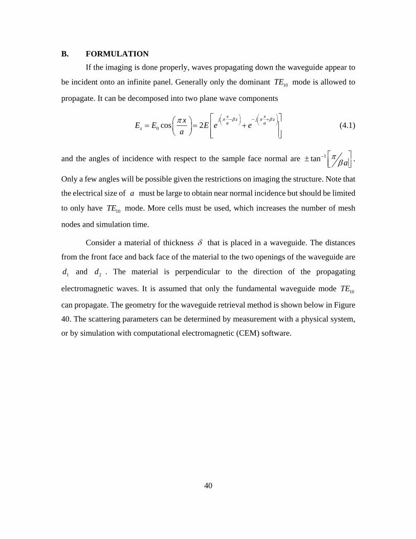
If the imaging is done properly, waves propagating down the waveguide appear to
be incident onto an infinite panel. Generally only the dominant 10TE mode is allowed to
propagate. It can be decomposed into two plane wave components
0 cos 2x xj z j za a
zxE E E e e
aπ β π βπ ⎛ ⎞ ⎛ ⎞− − +⎜ ⎟ ⎜ ⎟
⎝ ⎠ ⎝ ⎠⎡ ⎤⎛ ⎞= = +⎢ ⎥⎜ ⎟
⎝ ⎠ ⎢ ⎥⎣ ⎦ (4.1)
and the angles of incidence with respect to the sample face normal are 1tan aπ
β− ⎡ ⎤± ⎢ ⎥⎣ ⎦
.
Only a few angles will be possible given the restrictions on imaging the structure. Note that
the electrical size of a must be large to obtain near normal incidence but should be limited
to only have 10TE mode. More cells must be used, which increases the number of mesh
nodes and simulation time.
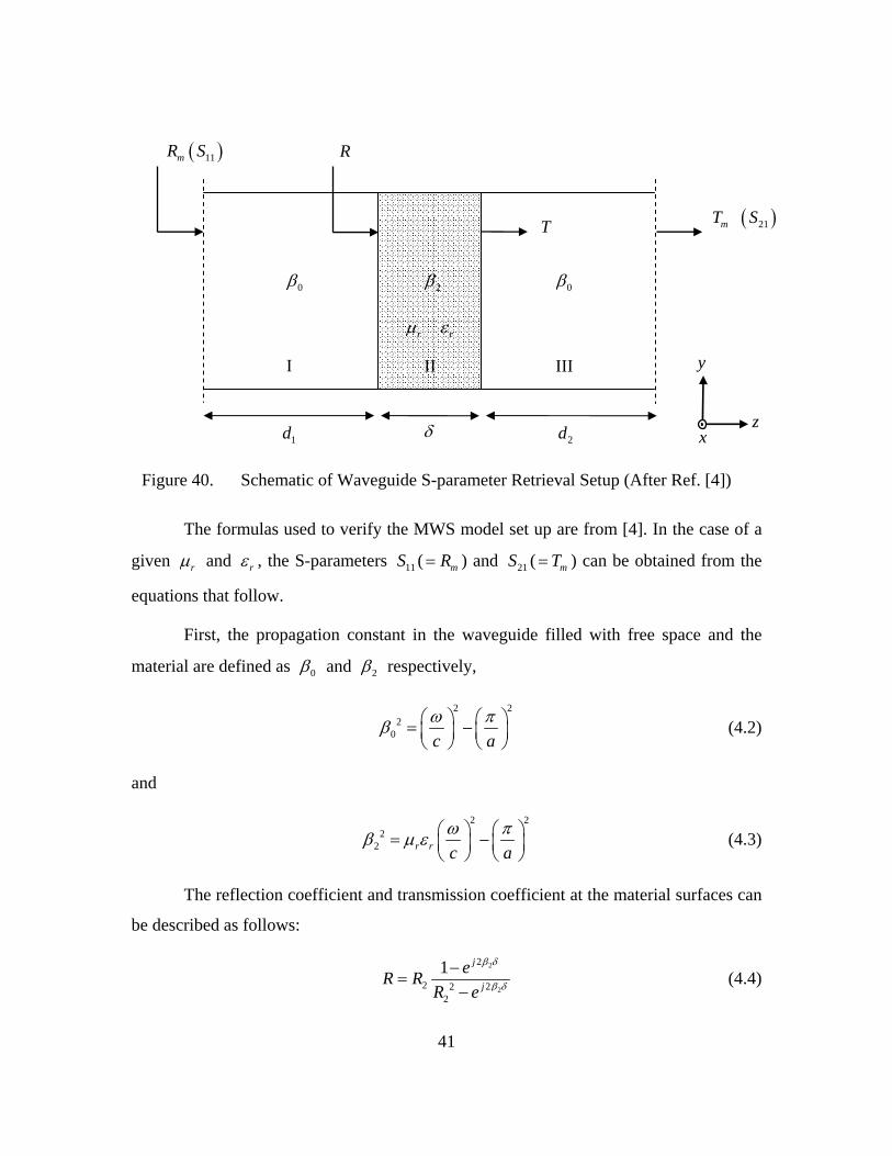
Consider a material of thickness δ that is placed in a waveguide. The distances
from the front face and back face of the material to the two openings of the waveguide are
1d and 2d . The material is perpendicular to the direction of the propagating
electromagnetic waves. It is assumed that only the fundamental waveguide mode 10TE
can propagate. The geometry for the waveguide retrieval method is shown below in Figure
40. The scattering parameters can be determined by measurement with a physical system,
or by simulation with computational electromagnetic (CEM) software.
41
Figure 40. Schematic of Waveguide S-parameter Retrieval Setup (After Ref. [4])
The formulas used to verify the MWS model set up are from [4]. In the case of a
given rµ and rε , the S-parameters 11S ( mR= ) and 21S ( mT= ) can be obtained from the
equations that follow.
First, the propagation constant in the waveguide filled with free space and the
material are defined as 0β and 2β respectively,
2 2
20 c a
ω πβ ⎛ ⎞ ⎛ ⎞= −⎜ ⎟ ⎜ ⎟⎝ ⎠ ⎝ ⎠
(4.2)
and
2 2
22 r r c a
ω πβ µ ε ⎛ ⎞ ⎛ ⎞= −⎜ ⎟ ⎜ ⎟⎝ ⎠ ⎝ ⎠
(4.3)
The reflection coefficient and transmission coefficient at the material surfaces can
be described as follows:
2
2
2
2 222
1 j
j
eR RR e
β δ
β δ
−=
− (4.4)
1d δ 2d
0β 0β2β
rµ rε
mR ( )11S R
T mT ( )21S
I II III
x
y
z

42
and
( )221jT e RRβ δ−= − (4.5)
with
0 22
0 2
r
r
R µ β βµ β β
−=
+ (4.6)
For the case where the waveguide is not fully filled, which is the case in Figure 40,
the distances between material surfaces and the openings of the waveguide 1d and 2d
must be included in the formula in order to have the correct phase of the S-parameters.
Therefore, the final reflection and transmission coefficients can be described as
0 1211
j dmS R Re β−= = (4.7)
and
( )0 1 221
j d dmS T Te β− += = (4.8)
This formula was compared to the MWS simulated S-parameters to make sure the
simulation set up in the waveguide was correct. The comparison is shown in the next
section.
The retrieval method used in the second part of this thesis is based on the approach
used by Zwick et al in [23], where the S-parameters are defined in terms of the reflection
and transmission coefficients as
0 1
22
11 2 2
(1 )1
j dR TS eR T
γ−−=
− (4.9)
( ) ( )0 1 2
2
21 2 2
11
j d dT RS e
R Tγ +−−
=−
(4.10)
Equations (4.9) and (4.10) can be solved for :R
2 2
11
11
42
K K SR
S± −
= (4.11)
43
with
2 211 21 1K S S= − + (4.12)
and
( )
11 21
11 211S S RT
R S S+ −
=− +
(4.13)
In Equation (4.11), the sign of the square root has to be chosen such that 1R ≤ .
The parameters γ and 0γ can be calculated as follows:
( )2 lnj k Tπγ
δ−
= (4.14)
and
2
20 0 0
122
j fa
γ π µ ε ⎛ ⎞= − ⎜ ⎟⎝ ⎠
(4.15)
with k being an integer value, f the frequency, and a the width of the waveguide. The
details on how to choose the correct k is described in [23]. Basically, k is first split into
a frequency-dependent part ( )k f and an offset 0k as follows:
( )0k k k f= + (4.16)
where ( )k f is simply determined by using the fact that the phase of T has to be
monotonically decreasing without large steps. The constant 0k can be obtained by finding
the 0k for which rε and rµ are almost constant over frequency. The complex
permeability and permittivity are finally determined as
( )( )0
0
11
RR
γµ µ
γ+
=−
(4.17)
and
44
2 2
2
12 2a
f
γπε
µ
⎛ ⎞ ⎛ ⎞−⎜ ⎟ ⎜ ⎟⎝ ⎠ ⎝ ⎠= (4.18)
C. RETRIEVAL USING NUMERICALLY GENERATED S-PARAMETERS
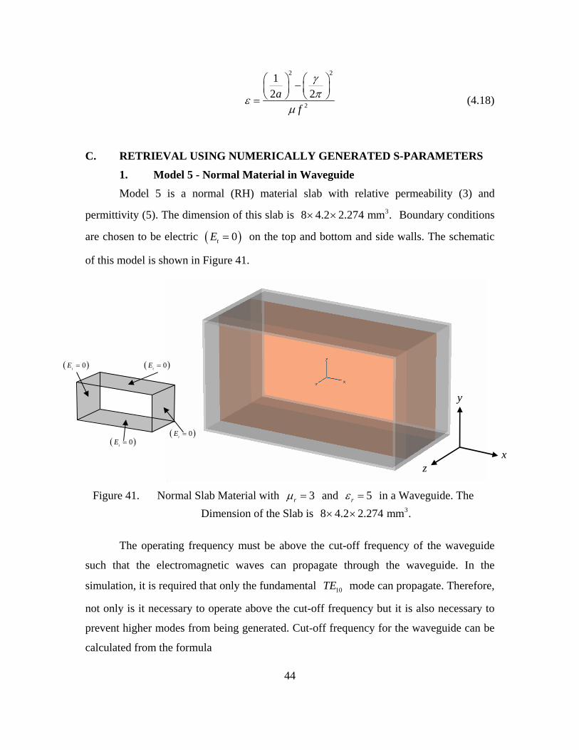
1. Model 5 - Normal Material in Waveguide Model 5 is a normal (RH) material slab with relative permeability (3) and
permittivity (5). The dimension of this slab is 38 4.2 2.274 mm .× × Boundary conditions
are chosen to be electric ( )0tE = on the top and bottom and side walls. The schematic
of this model is shown in Figure 41.
Figure 41. Normal Slab Material with 3rµ = and 5rε = in a Waveguide. The
Dimension of the Slab is 38 4.2 2.274 mm .× ×
The operating frequency must be above the cut-off frequency of the waveguide
such that the electromagnetic waves can propagate through the waveguide. In the
simulation, it is required that only the fundamental 10TE mode can propagate. Therefore,
not only is it necessary to operate above the cut-off frequency but it is also necessary to
prevent higher modes from being generated. Cut-off frequency for the waveguide can be
calculated from the formula
z
y
x
( )0tE =
( )0tE =
( )0tE =
( )0tE =
45
( )2 21
2c mn
m nfa bµε
⎛ ⎞ ⎛ ⎞= +⎜ ⎟ ⎜ ⎟⎝ ⎠ ⎝ ⎠
(Hz) (4.19)
For this model, the width of the waveguide is 8 mma = and the height of the
waveguide is 4.2 mm,b = and 0µ µ= and 0ε ε= for free space. The operating
frequency range for this waveguide can be chosen from Table 2.
( )c mnf m =1 m =2 m =3
n =0 18.74 GHz 37.48 GHz 56.22 GHz
n =1 40.32 GHz 51.76 GHz 66.60 GHz
n =2 73.81 GHz 80.64 GHz 90.88 GHz
n =3 108.72 GHz 113.46 GHz 120.96 GHz
Table 2. Cut-off Frequencies for Waveguide with 8 mma = and 4.2 mmb = .
According to Table 2, the operating frequency should be chosen between 18.74
and 37.48 GHz to only allow the 10TE mode to propagate.
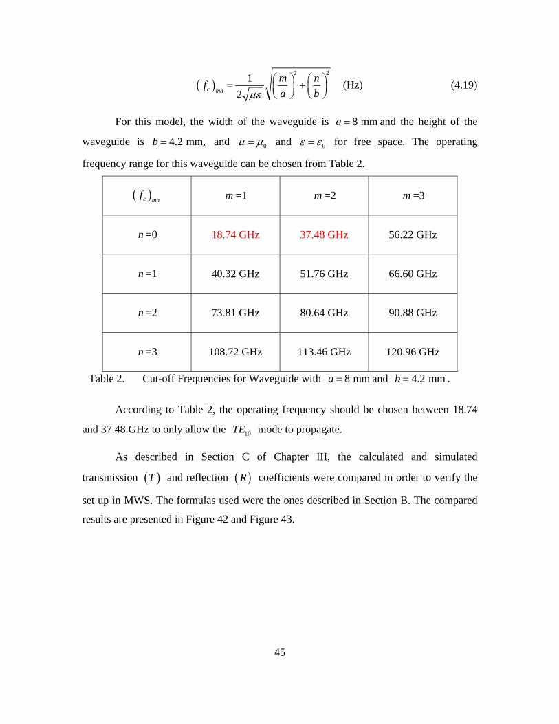
As described in Section C of Chapter III, the calculated and simulated
transmission ( )T and reflection ( )R coefficients were compared in order to verify the
set up in MWS. The formulas used were the ones described in Section B. The compared
results are presented in Figure 42 and Figure 43.
46
Figure 42. (a) Magnitude Differences of Transmission Coefficient between the
Calculated and Simulated Data (b) Phase Differences (Degrees) of Transmission Coefficient between the Calculated and Simulated Data
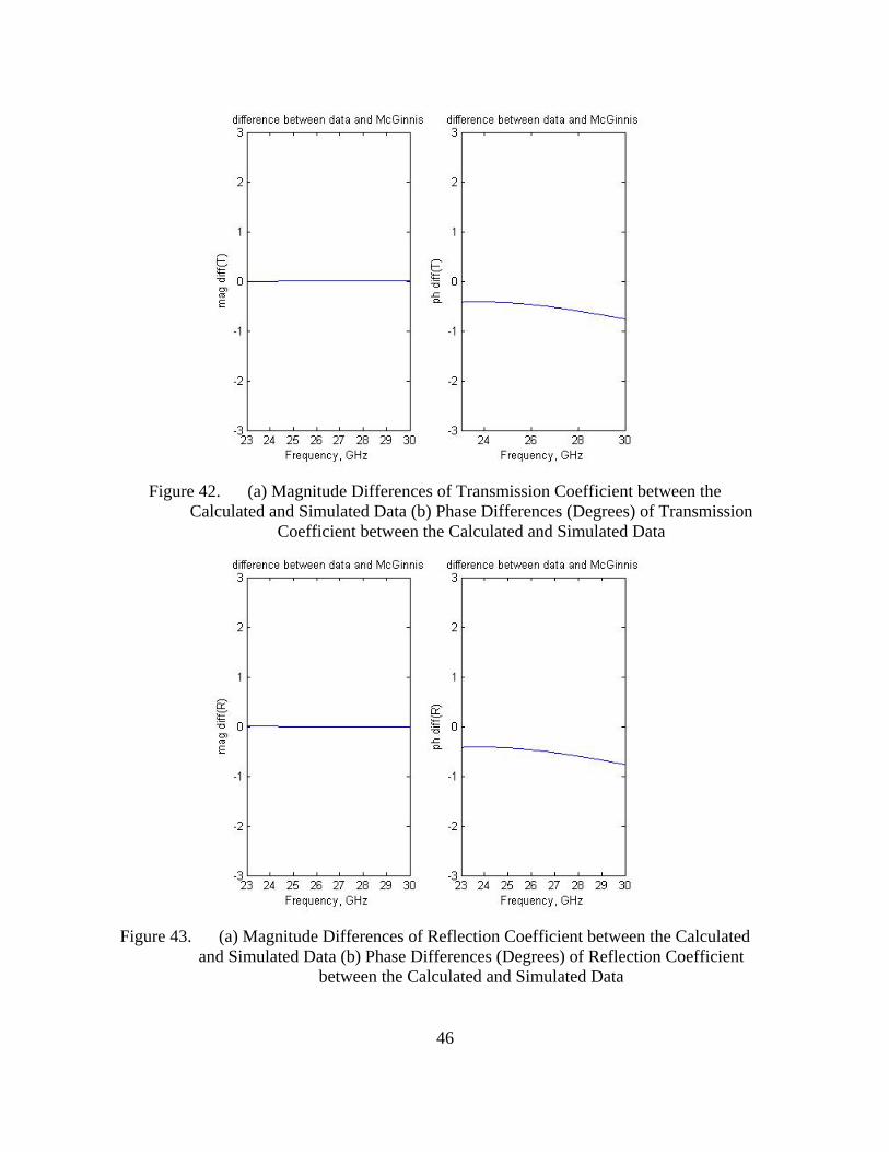
Figure 43. (a) Magnitude Differences of Reflection Coefficient between the Calculated
and Simulated Data (b) Phase Differences (Degrees) of Reflection Coefficient between the Calculated and Simulated Data
47
According to the Figures 42 and 43, the differences between the calculated and
simulated data for the real parts of the transmission and reflection coefficients are almost
zero. There is less than a one degree phase difference in both the transmission and
reflection coefficients, which is acceptable. Therefore, the simulation set up is considered
correct and the results are acceptable.
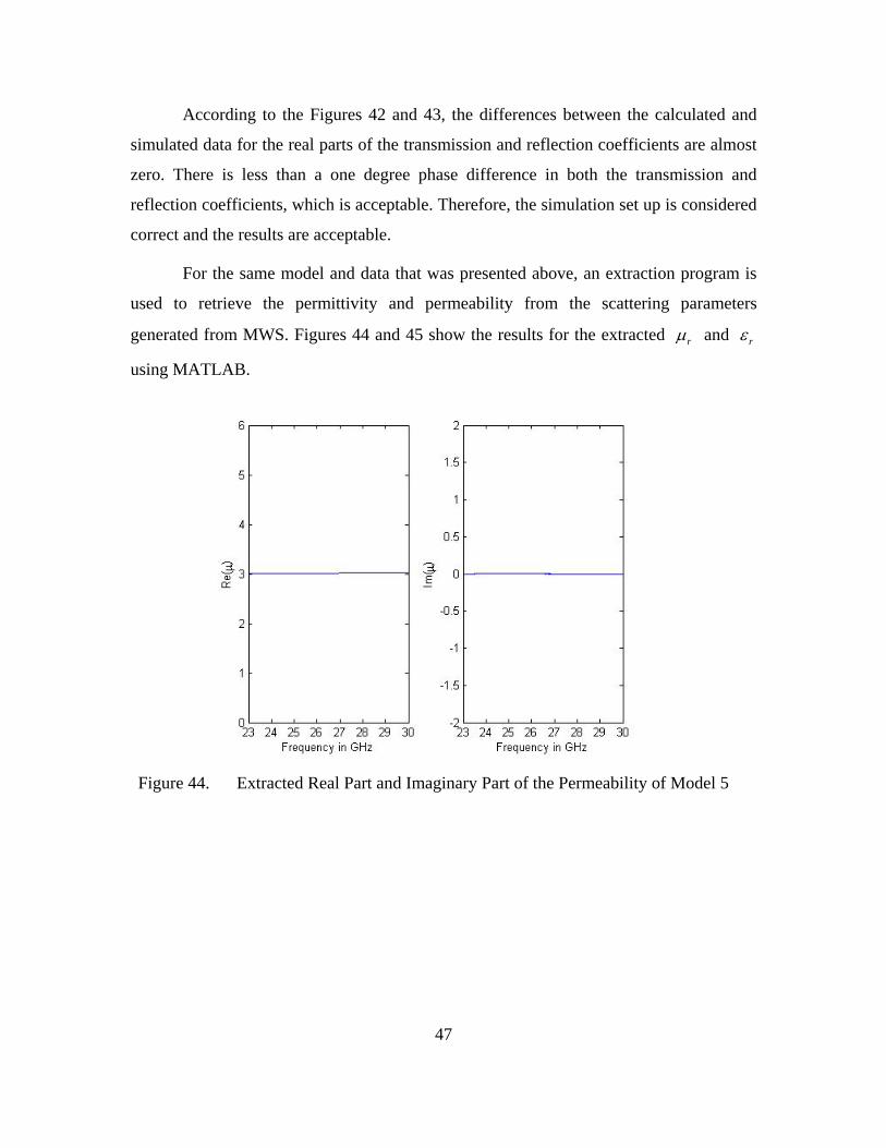
For the same model and data that was presented above, an extraction program is
used to retrieve the permittivity and permeability from the scattering parameters
generated from MWS. Figures 44 and 45 show the results for the extracted rµ and rε
using MATLAB.
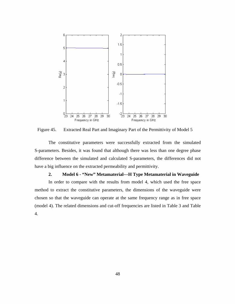
Figure 44. Extracted Real Part and Imaginary Part of the Permeability of Model 5
48
Figure 45. Extracted Real Part and Imaginary Part of the Permittivity of Model 5
The constitutive parameters were successfully extracted from the simulated
S-parameters. Besides, it was found that although there was less than one degree phase
difference between the simulated and calculated S-parameters, the differences did not
have a big influence on the extracted permeability and permittivity.
2. Model 6 - “New” Metamaterial---H Type Metamaterial in Waveguide In order to compare with the results from model 4, which used the free space
method to extract the constitutive parameters, the dimensions of the waveguide were
chosen so that the waveguide can operate at the same frequency range as in free space
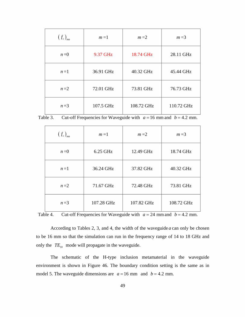
(model 4). The related dimensions and cut-off frequencies are listed in Table 3 and Table
4.
49
( )c mnf m =1 m =2 m =3
n =0 9.37 GHz 18.74 GHz 28.11 GHz
n =1 36.91 GHz 40.32 GHz 45.44 GHz
n =2 72.01 GHz 73.81 GHz 76.73 GHz
n =3 107.5 GHz 108.72 GHz 110.72 GHz
Table 3. Cut-off Frequencies for Waveguide with 16 mma = and 4.2 mm.b =
( )c mnf m =1 m =2 m =3
n =0 6.25 GHz 12.49 GHz 18.74 GHz
n =1 36.24 GHz 37.82 GHz 40.32 GHz
n =2 71.67 GHz 72.48 GHz 73.81 GHz
n =3 107.28 GHz 107.82 GHz 108.72 GHz
Table 4. Cut-off Frequencies for Waveguide with 24 mma = and 4.2 mm.b =
According to Tables 2, 3, and 4, the width of the waveguide a can only be chosen
to be 16 mm so that the simulation can run in the frequency range of 14 to 18 GHz and
only the 10TE mode will propagate in the waveguide.
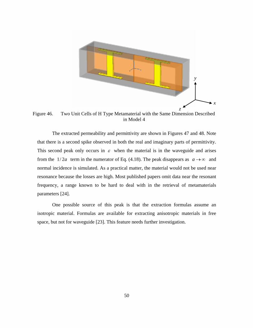
The schematic of the H-type inclusion metamaterial in the waveguide
environment is shown in Figure 46. The boundary condition setting is the same as in
model 5. The waveguide dimensions are 16 mma = and 4.2 mm.b =
50
Figure 46. Two Unit Cells of H Type Metamaterial with the Same Dimension Described
in Model 4
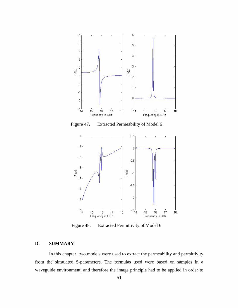
The extracted permeability and permittivity are shown in Figures 47 and 48. Note
that there is a second spike observed in both the real and imaginary parts of permittivity.
This second peak only occurs in ε when the material is in the waveguide and arises
from the 1/ 2a term in the numerator of Eq. (4.18). The peak disappears as a → ∞ and
normal incidence is simulated. As a practical matter, the material would not be used near
resonance because the losses are high. Most published papers omit data near the resonant
frequency, a range known to be hard to deal with in the retrieval of metamaterials
parameters [24].
One possible source of this peak is that the extraction formulas assume an
isotropic material. Formulas are available for extracting anisotropic materials in free
space, but not for waveguide [23]. This feature needs further investigation.
z
y
x
51
Figure 47. Extracted Permeability of Model 6
Figure 48. Extracted Permittivity of Model 6
D. SUMMARY
In this chapter, two models were used to extract the permeability and permittivity
from the simulated S-parameters. The formulas used were based on samples in a
waveguide environment, and therefore the image principle had to be applied in order to

52
treat the model as an infinite slab. Test cases were performed to verify the effectiveness of
the simulation set up. It was found that the differences between the simulated and
calculated S-parameter were negligible. Again, the resonant frequency of the metamaterial
model was very sensitive to the mesh cell number; therefore, it is good to have both
simulation and measurement data to compare. The models have shown that the waveguide
environment program can work not only for normal materials but also metamaterials. In
comparing model 4 with model 6, the extracted permeability and permittivity were very
close. This result showed that both the free space and waveguide method can be used to
retrieve the constitutive parameters of materials.
53
V. CONCLUSION
A. SUMMARY AND CONCLUSIONS The basic concept of a metamaterial and the unusual properties of DNG materials
were discussed. The applications of metamaterials in waveguide miniaturization,
microwave devices and other possible applications were presented and explained. To
employ metamaterials in devices it is necessary to know their effective permittivity and
permeability. The information can be obtained by measurements on a sample in free space
or waveguide. Alternately, simulation of the material in free space or a waveguide could be
used.
The equations used in the free space environment to extract the constitutive
parameters from simulated S-parameters were described and programmed in MATLAB.
Test cases were used to validate the correctness of the simulation settings. Several different
types of materials, including the normal (homogeneous) material and metamaterial were
simulated in MWS and a retrieval program was used to extract the permittivity and
permeability of the materials. The results were compared with published data. The resonant
frequency of the results and its relationship to the dimensions of the inclusions and number
of mesh cells at the simulation starting point was investigated and discussed.
The waveguide environment retrieval method and accompanying equations were
discussed in Chapter IV. Boundary conditions were properly selected so that a small
sample in the waveguide environment could be treated as an infinite panel. The same
metamaterial (H-type inclusions) was examined using both the free space and waveguide
methods to compare the extracted results.
It was shown that both the free space and waveguide methods could be used to
successfully retrieve the constitutive parameters from the scattering parameters. In both
free space and waveguide cases the number of mesh cells used at the simulation starting
point, the dimensions of the inclusions, and the boundary condition settings in MWS were
the key parameters for successful retrieval.

54
Finally, the simulation and extracted results of the effective parameters could be
used as data for designing microwave devices with metamaterials. The simulation methods
and extraction programs make the effective parameter determination much more efficient
in time and cost than building large panels for testing.
B. FUTURE WORK
In this thesis, normal and DNG materials were used to examine the retrieval
programs. Single negative materials (SNG) were not included. Dealing with the SNG
materials is more of a challenge because of the sign ambiguity in the square root of µ ε⋅
when it is programmed. More inputs must be acquired to decide the correct sign when
using SNG materials. Future research could be conducted to validate the programs using
thicker materials which are more realistic in terms of fabrication. In this research the
sample thickness has been small compared to wavelength. This condition avoids many
ambiguities that occur for thick samples. Future work could also be conducted to correct
the errors due to the nonzero incidence so that the extracted results could be compared with
the normal incident cases. Finally, the cause of the second resonance in ε that occurs in
the waveguide needs to be examined further.

55
APPENDIX
A. MATLAB CODE FOR FREE SPACE ENVIRONMENT This appendix provides the MATLAB code used to retrieve the constitutive
parameters from S-parameters in Chapter III. The code is written in MATLAB 7. This code
retrieves and plots rµ , rε , n, and Z as a function of frequency respectively.
%###################################################### % multiple frequency for plane wave incident on a panel % sample has thickness d, free space case %###################################################### clear clc %*************************************************** % constants rad=pi/180; eps0=8.85e-12; mu0=4*pi*1e-7; eta0=sqrt(mu0/eps0); % free space c=1/sqrt(eps0*mu0); %*************************************************** % variables d=2.5e-3; % thickness of the sample f1=2e9; df=18e6; f2=20e9; Nf=floor((f2-f1)/df)+1; % frequency range and spacing %*************************************************** % load raw data load M1r.m; load M2r.m; load P1r.m; load P2r.m; Mag1=M1r(:,2); Mag2=M2r(:,2); Ph1=-unwrap(P1r(:,2),180); Ph2=-unwrap(P2r(:,2),180); %***************************************** % freqyency loop begin for it=1:Nf f=f1+(it-1)*df; Fr(it)=f; Fghz(it)=f/1e9; fghz=f/1e9; Z0=eta0; W=2*pi*Fr(it); beta0=W/c; %******************************************* % combine magnitude and phase of the S11 and S21 R(it)=Mag1(it)*exp(j*Ph1(it)*rad); T(it)=Mag2(it)*exp(j*Ph2(it)*rad); %*******************************************
56
% m loop begin Max=0; % ---------m value set up itt=0; for m=-Max:Max itt=itt+1; %*************************************************** % using formulas from Robust method Tp=T(it); Z21(it)=sqrt(((1+R(it))^2-Tp^2)/((1-R(it))^2-Tp^2)); Z22(it)=-sqrt(((1+R(it))^2-Tp^2)/((1-R(it))^2-Tp^2)); expinkd1(it)=Tp/(1-R(it)*(Z21(it)-1)/(Z21(it)+1)); expinkd2(it)=Tp/(1-R(it)*(Z22(it)-1)/(Z22(it)+1)); if abs(real(Z21(it)))>=0.005 & real(Z21(it))>=0 expinkd(it)=expinkd1(it); Z2(it)=Z21(it); end if abs(real(Z21(it)))>=0.005 & real(Z21(it))<0 expinkd(it)=expinkd2(it); Z2(it)=Z22(it); end if abs(real(Z21(it)))<0.005 & abs(expinkd1(it))<=1 expinkd(it)=expinkd1(it); Z2(it)=Z21(it); end if abs(real(Z21(it)))<0.005 & abs(expinkd1(it))>1 expinkd(it)=expinkd2(it); Z2(it)=Z22(it); end ni(it)=-1/(beta0*d)*j*real(log(expinkd(it))); % imag of n nr(it,itt)=1/(beta0*d)*(imag(log(expinkd(it)))+2*m*pi); %real of n n2(it,itt)=nr(it,itt)+ni(it); Er2(it,itt)=n2(it,itt)/Z2(it); Mr2(it,itt)=n2(it,itt)*Z2(it); end % end of m loop end % end of frequency loop figure(1) subplot(121); plot(Fghz,real(Mr2)); xlabel('Frequency in GHz') ylabel('Re(\mu)') subplot(122) plot(Fghz,imag(Mr2)); xlabel('Frequency in GHz') ylabel('Im(\mu)') figure(2) subplot(121); plot(Fghz,real(Er2)); xlabel('Frequency in GHz') ylabel('Re(\epsilon)') subplot(122) plot(Fghz,imag(Er2)); xlabel('Frequency in GHz') ylabel('Im(\epsilon)')
57
figure(3) subplot(121); plot(Fghz,real(n2)); xlabel('Frequency in GHz') ylabel('Re(n)') subplot(122) plot(Fghz,imag(n2)); xlabel('Frequency in GHz') ylabel('Im(n)') figure(4) subplot(121); plot(Fghz,real(Z2)); xlabel('Frequency in GHz') ylabel('Re(Z)') subplot(122) plot(Fghz,imag(Z2)); xlabel('Frequency in GHz') ylabel('Im(Z)')

58
B. MATLAB CODE FOR WAVEGUIDE ENVIRONMENT
This appendix provides the MATLAB code used to retrieve the constitutive
parameters from S-parameters in Chapter IV. The code is written in MATLAB 7. This
code retrieves and plots rµ , rε , n, and Z as a function of frequency respectively.
%####################################################################### % multiple frequency in a waveguide environment % sample has thickness delta, total length of the waveguide is d1+delta+d2 %####################################################################### clear clc a=16e-3; delta=2.274e-3; d1=1e-3; d2=1e-3; eps0=8.85e-12; mu0=4*pi*1e-7; c=1/sqrt(eps0*mu0); rad=pi/180; Z0=377; %************************************************* load M1r.m; load M2r.m; load P1r.m; load P2r.m; Mag1=M1r(:,2); Mag2=M2r(:,2); Ph1=-unwrap(P1r(:,2),180); Ph2=-unwrap(P2r(:,2),180); %************************************************* it=0; f1=14e9; df=4e6; f2=18e9; Nf=floor((f2-f1)/df)+1; for it=1:Nf f=f1+(it-1)*df; % must higher than the cut-off frequency in free space Fr(it)=f; w=2*pi*Fr(it); wave=c/f; Rm(it)=Mag1(it)*exp(j*Ph1(it)*rad); Tm(it)=Mag2(it)*exp(j*Ph2(it)*rad); beta0(it)=sqrt((w/c)^2-(pi/a)^2); end %********************************************************* % make use of equation from Thomas nfreq=it; for it=1:nfreq Tt(it)=Tm(it)*exp(-j*beta0(it)*(d1+d2)); %---T Rr(it)=Rm(it)*exp(-j*2*beta0(it)*d1); %---R %***************************************************** % to get Z2 b=(Rr(it)^2-Tt(it)^2+1)/(2*Rr(it)); R21=b+(sqrt(b^2-1)); R22=b-(sqrt(b^2-1));
59
Rn=nan; if abs(R21)<=1 RR=R21; Rn=RR; %---R2 end if abs(R22)<=1 RR=R22; Rn=RR; end if (abs(R21)<1 & abs(R22)<1) | (abs(R21)==1 & abs(R22)==1) disp(['both solutions give |R|<1 for fghz = ',num2str(fghz)]) end Z=(1+RR)/(1-RR); sgn=1; if real(Z)<0, sgn=-1; end Z2(it)=Z*sgn; %------------------------------------------------------------------ k=0; % need to be determined %------------------------------------------------------------------ K=Rr(it)^2-Tt(it)^2+1; r1=(K+sqrt(K^2-4*Rr(it)^2))/2/Rr(it); r2=(K-sqrt(K^2-4*Rr(it)^2))/2/Rr(it); if abs(r1)<=1 r=r1; end if abs(r2)<=1 r=r2; end t=(Rr(it)+Tt(it)-r)/(1-r*(Rr(it)+Tt(it))); gamma=(j*2*k*pi-log(t))/delta; gamma0=-j*2*pi*sqrt(Fr(it)^2*mu0*eps0-(1/2/a)^2); Mr(it)=mu0*(gamma*(1+r)/gamma0/(1-r)); Er(it)=(((1/2/a)^2-(gamma/2/pi)^2)/Mr(it)/Fr(it)^2); Mre(it)=Mr(it)/mu0; Ere(it)=Er(it)/eps0; n2(it)=Mre(it)/Z2(it); end % end of frequency loop figure(1) subplot(121); plot(Fr/1e9,real(Mre)); xlabel('Frequency in GHz') ylabel('Re(\mu)') subplot(122) plot(Fr/1e9,imag(Mre)); xlabel('Frequency in GHz') ylabel('Im(\mu)') figure(2) subplot(121); plot(Fr/1e9,real(Ere)); xlabel('Frequency in GHz') ylabel('Re(\epsilon)') subplot(122) plot(Fr/1e9,imag(Ere)); xlabel('Frequency in GHz') ylabel('Im(\epsilon)')
60
figure(3) subplot(121); plot(Fr/1e9,real(n2)); xlabel('Frequency in GHz') ylabel('Re(n)') subplot(122) plot(Fr/1e9,imag(n2)); xlabel('Frequency in GHz') ylabel('Im(n)') figure(4) subplot(121); plot(Fr/1e9,real(Z2)); xlabel('Frequency in GHz') ylabel('Re(Z)') subplot(122) plot(Fr/1e9,imag(Z2)); xlabel('Frequency in GHz') ylabel('Im(Z)')
61
LIST OF REFERENCES
1. Hannan, P. W. & Balfour, M. A., “Simulation of a Phased-Array Antenna in Waveguide,” IEEE Trans. on Antennas and Propagation. Vol. 13, Issue 3, May 1965 Page(s):342 - 353.
2. McGinnis, Dave, “Electromagnetic Properties of ECCOSORB MF-190,” Pbar Note 566 (www-bdnew.fnal.gov/pbar), May 1997.
3. Sun, Ding, “Measurement of Complex Permittivity and Permeability of Microwave Absorber ECCOSORB MF-190,” Pbar Note 576 (www-bdnew.fnal.gov/pbar), August 1997.
4. McGinnis, Dave, “Measurement of Relative Permittivity and Permeability Using Two Port S-parameter Technique,” Pbar Note 585 (www-bdnew.fnal.gov/pbar), April 1998.
5. Zwick, Thomas, Chandrasekhar, Arun, Baks, Christian W., Pfeiffer, Ullrich R., Brebels, Steven, & Gaucher, Brian P., “Determination of the Complex Permittivity of Packaging Materials at Millimeter-Wave Frequencies,” IEEE Trans. Microwave Theory Tech. 54, No. 3, (2006).
6. Jenn, D., Notes for EC3630 (Radiowave Propagation), Naval Postgraduate School, 2003 (unpublished).
7. Veselago, V. G., “The Electrodynamics of Substances with Simultaneously Negative Values of µ and ε ,” Sov. Phys. Usp., 10, 509, (1968).
8. Pendry, J. B., Holden, A. J., Stewart, W. J., & Young, I., “Extremely Low Frequency Plasmons in Metallic Mesostructures,” Phys. Rev. Lett., 76, 4773, (1996).
9. Pendry, J. B., Holden, A. J., Robbins, D. J., & Stewart, W. J., “Magnetism from conductors and enhanced nonlinear phenomena,” IEEE Trans. Microwave Theory Tech., 47, 2075, (1999).
10. Pendry, J. B., “Negative Refraction Makes a Perfect Lens,” Phys. Rev. Lett., 85, 3966, (2000).
11. Smith, D. R., Padilla, Willie J., Vier, D. C., Nemat-Nasser, S. C., & Schultz, S., “Composite Medium with Simultaneously Negative Permeability and Permittivity,” Phys. Rev. Lett., 84, 4184, (2000).
12. Shelby, R. A., Smith, D. R., & Schultz, S., “Experimental Verification of a Negative Index of Refraction,” Science, 292, 77, (2001).
62
13. Ziolkowski, R. W. & Engheta, N., “A positive future for double-negative metamaterials,” IEEE Trans. Microwave Theory Tech., 53, No. 4, (2005).
14. Smith, D. R., Pendry, J. B., & Wiltshire, M. C. K., “Metamaterials and Negative Refractive Index,” Science, Vol. 305 (2004).
15. Hrabar, Silvio, Bartolic, Juraj, & Sipus, Zvonimir, “Waveguide Miniaturization Using Uniaxial Negative Permeability Metamaterial,” IEEE Trans. on Antennas and Propagation., 53, No. 1, (2005).
16. Jakšic´, Zoran, Dalarsson, Nils, & Maksimovic´, Milan, “Negative Refractive Index Metamaterials: Principles and Applications,” Microwave Review, Jun. 2006.
17. Elefttheriades, G. V., “Negative-Refractive-Index Transmission-Line Metamaterials and Enabling Microwave Devices,” The Radio Science Bulletin, No. 312 (2005).
18. Cotuk, Unit, “Scattering from Multi-layered Metamaterials Using Wave Matrices,” Naval Postgraduate School Thesis, Sept. 2005.
19. Chen, Xudong, Grzegorczyk, Tomasz M., Wu, Bae-Ian, Pacheco Jr., Joe, & Kong, Jin Au, “Robust Method to Retrieve the Constitutive Effective Parameters of Metamaterials,” Phys. Rev. E., 70, 016608, (2004).
20. Smith, D. R., Vier, D. C., Koschny, Thomas, & Soukoulis, C. M., “Electromagnetic Parameter Retrieval from inhomogeneous metamaterials,” Phys. Rev. E., 71, 036617, (2005).
21. Zhou, Jiangfeng, Zang, Lei, Tuttle, Gary, Koschny, Thomas, & Soukoulis, Costas M., “Negative index materials using simple short wire pairs,” Phys. Rev. B., 73, 041101, (2006).
22. Zhou, Jiangfeng, Koschny, Thomas, Zhang, Lei, Tuttle, Gary, & Soukoulis, Costas M., “Experimental demonstration of negative index of refraction,” Applied Phys. Lett., 88, 221103, (2006).
23. Zwick, Thomas, Chandrasekhar, Arun, Baks, Christian W., Pfeiffer, Ullrich R., Brebels, Steven, & Gaucher, Brian P., “Determination of the Complex Permittivity of Packaging Materials at Millimeter-Wave Frequencies,” IEEE Trans. Microwave Theory Tech., 54, No. 3, (2006).
24. Chen, Xudong, Wu, Bae-Ian, Kong, Jin Au, & Grzegorczyk, Tomasz M., “Retrieval of the Effective Constitutive Parameters of Bianisotropic Metamaterials,” Phys. Rev. E., 71, 046610, (2005).
63
INITIAL DISTRIBUTION LIST
1. Defense Technical Information Center Ft. Belvoir, Virginia
2. Dudley Knox Library Naval Postgraduate School Monterey, California
3. Chairman Information Sciences Department Monterey, California
4. Professor David C. Jenn Department of Electrical and Computer Engineering Monterey, California
5. Professor Michael A. Morgan Department of Electrical and Computer Engineering Monterey, California
6. C.S.I.S.T. Library Taoyuan, Taiwan R.O.C.