Nature, Not Human Activity,Rules the Climate

© 2008, Science and Environmental Policy Project / S. Fred Singer

Published by THE HEARTLAND INSTITUTE19 South LaSalle Street #903

Chicago, Illinois 60603 U.S.A.phone 312/377-4000

fax 312/377-5000www.heartland.org

All rights reserved, including the right to reproducethis book or portions thereof in any form.

Opinions expressed are solely those of the authors.Nothing in this report should be construed as reflecting the views of

the Science and Environmental Policy Project or The Heartland Institute,or as an attempt to influence pending legislation.

Please use the following reference to this report:

S. Fred Singer, ed., Nature, Not Human Activity, Rules the Climate: Summary for Policymakers of theReport of the Nongovernmental International Panel on Climate Change, Chicago, IL: The Heartland

Institute, 2008.

Printed in the United States of America978-1-934791-01-1

1-934791-01-6

Second printing: April 2008

Nature, Not Human Activity,Rules the Climate

Summary for Policymakers of the Report of theNongovernmental International Panel on Climate Change

Edited by S. Fred Singer

Contributors

Warren AndersonUnited States

Dennis AveryUnited States

Franco BattagliaItaly

Robert CarterAustralia

Richard CourtneyUnited Kingdom

Joseph D’AleoUnited States

Fred GoldbergSweden

Vincent GrayNew Zealand

Kenneth HaapalaUnited States

Klaus HeissAustria

Craig IdsoUnited States

Zbigniew JaworowskiPoland

Olavi KärnerEstonia

Madhav KhandekarCanada

William KininmonthAustralia

Hans LabohmNetherlands

Christopher MoncktonUnited Kingdom

Lubos MotlCzech Republic

Tom SegalstadNorway

S. Fred SingerUnited States

George TaylorUnited States

Dick ThoenesNetherlands

Anton UriarteSpain

Gerd WeberGermany

Published for the Nongovernmental International Panel on Climate Change

by

iii

ForewordIn his speech at the United Nations’ climateconference on September 24, 2007, Dr. VaclavKlaus, president of the Czech Republic, said itwould most help the debate on climate change if thecurrent monopoly and one-sidedness of thescientific debate over climate change by theIntergovernmental Panel on Climate Change (IPCC)were eliminated. He reiterated his proposal that theUN organize a parallel panel and publish twocompeting reports.

The present report of the NongovernmentalInternational Panel on Climate Change (NIPCC)does exactly that. It is an independent examinationof the evidence available in the published,peer-reviewed literature – examined without biasand selectivity. It includes many research papersignored by the IPCC, plus additional scientificresults that became available after the IPCCdeadline of May 2006.

The IPCC is pre-programmed to produce reportsto support the hypotheses of anthropogenic warmingand the control of greenhouse gases, as envisionedin the Global Climate Treaty. The 1990 IPCCSummary completely ignored satellite data, sincethey showed no warming. The 1995 IPCC reportwas notorious for the significant alterations made tothe text after it was approved by the scientists – inorder to convey the impression of a humaninfluence. The 2001 IPCC report claimed thetwentieth century showed ‘unusual warming’ basedon the now-discredited hockey-stick graph. Thelatest IPCC report, published in 2007, completelydevaluates the climate contributions from changesin solar activity, which are likely to dominate anyhuman influence.

The foundation for NIPCC was laid five yearsago when a small group of scientists from theUnited States and Europe met in Milan during oneof the frequent UN climate conferences. But it gotgoing only after a workshop held in Vienna in April2007, with many more scientists, including somefrom the Southern Hemisphere.

The NIPCC project was conceived and directedby Dr. S. Fred Singer, professor emeritus ofenvironmental sciences at the University ofVirginia. He should be credited with assembling asuperb group of scientists who helped put thisvolume together.

Singer is one of the most distinguished

scientists in the U.S. In the 1960s, he establishedand served as the first director of the U.S. WeatherSatellite Service, now part of the NationalOceanographic and Atmospheric Administration(NOAA), and earned a U.S. Department ofCommerce Gold Medal Award for his technicalleadership. In the 1980s, Singer served for fiveyears as vice chairman of the National AdvisoryCommittee for Oceans and Atmosphere (NACOA)and became more directly involved in globalenvironmental issues.

Since retiring from the University of Virginiaand from his last federal position as chief scientistof the Department of Transportation, Singerfounded and directed the nonprofit Science andEnvironmental Policy Project, an organization I ampleased to serve as chair. SEPP’s major concern hasbeen the use of sound science rather thanexaggerated fears in formulating environmentalpolicies.

Our concern about the environment, going backsome 40 years, has taught us important lessons. It isone thing to impose drastic measures and harsheconomic penalties when an environmental problemis clear-cut and severe. It is foolish to do so whenthe problem is largely hypothetical and notsubstantiated by observations. As NIPCC shows byoffering an independent, non-governmental ‘secondopinion’ on the ‘global warming’ issue, we do notcurrently have any convincing evidence orobservations of significant climate change fromother than natural causes.

Frederick SeitzPresident Emeritus, Rockefeller UniversityPast President, National Academy of SciencesPast President, American Physical SocietyChairman, Science and Environmental Policy

Project

February 2008

Dr. Seitz passed away on March 2, 2008 at the ageof 96. He will be greatly missed by all of us whoknew and admired him.

iv

PrefaceBefore facing major surgery, wouldn’t you want asecond opinion?

When a nation faces an important decision thatrisks its economic future, or perhaps the fate of theecology, it should do the same. It is a time-honoredtradition in this case to set up a ‘Team B,’ whichexamines the same original evidence but may reacha different conclusion. The NongovernmentalInternational Panel on Climate Change (NIPCC)was set up to examine the same climate data used bythe United Nations-sponsored IntergovernmentalPanel on Climate Change (IPCC).

On the most important issue, the IPCC’s claimthat “most of the observed increase in globalaverage temperatures since the mid-20th century isvery likely (defined by the IPCC as between 90 to99 percent certain) due to the observed increase inanthropogenic greenhouse gas concentrations,”(emphasis in the original), NIPCC reaches theopposite conclusion – namely, that natural causesare very likely to be the dominant cause. Note: Wedo not say anthropogenic greenhouse (GH) gasescannot produce some warming. Our conclusion isthat the evidence shows they are not playing asignificant role.

Below, we first sketch out the history of the twoorganizations and then list the conclusions andresponses that form the body of the NIPCC report.

A Brief History of the IPCCThe rise in environmental consciousness since the1970s has focused on a succession of ‘calamities’:cancer epidemics from chemicals, extinction ofbirds and other species by pesticides, the depletionof the ozone layer by supersonic transports and laterby freons, the death of forests (‘Waldsterben’)because of acid rain, and finally, global warming,the “mother of all environmental scares” (accordingto the late Aaron Wildavsky).

The IPCC can trace its roots to World EarthDay in 1970, the Stockholm Conference in 1971-72,and the Villach Conferences in 1980 and 1985. InJuly 1986, the United Nations EnvironmentProgram (UNEP) and the World MeteorologicalOrganization (WMO) establ ished theIntergovernmental Panel on Climate Change (IPCC)as an organ of the United Nations.

The IPCC’s key personnel and lead authors

were appointed by governments, and its Summariesfor Policymakers (SPM) have been subject toapproval by member governments of the UN. Thescientists involved with the IPCC are almost allsupported by government contracts, which pay notonly for their research but for their IPCC activities.Most travel to and hotel accommodations at exoticlocations for the drafting authors is paid withgovernment funds.

The history of the IPCC has been described inseveral publications. What is not emphasized,however, is the fact that it was an activist enterprisefrom the very beginning. Its agenda was to justifycontrol of the emission of greenhouse gases,especially carbon dioxide. Consequently, itsscientific reports have focused solely on evidencethat might point toward human-induced climatechange. The role of the IPCC “is to assess on acomprehensive, objective, open and transparentbasis the latest scientific, technical andsocio-economic literature produced worldwiderelevant to the understanding of the risk ofhuman-induced climate change, its observed andprojected impacts and options for adaptation andmitigation” (emphasis added) [IPCC 2008].

The IPCC’s three chief ideologues have been(the late) Professor Bert Bolin, a meteorologist atStockholm University; Dr. Robert Watson, anatmospheric chemist at NASA, later at the WorldBank, and now chief scientist at the UK Departmentof Environment, Food and Rural Affairs; and Dr.John Houghton, an atmospheric radiation physicistat Oxford University, later head of the UK MetOffice as Sir John Houghton.

Watson had chaired a self-appointed group tofind evidence for a human effect on stratosphericozone and was instrumental in pushing for the 1987Montreal Protocol to control the emission ofchlorofluorocarbons (CFCs). Using the blueprint ofthe Montreal Protocol, environmental lawyer DavidDoniger of the Natural Resources Defense Councilthen laid out a plan to achieve the same kind ofcontrol mechanism for greenhouse gases, a plan thateventually was adopted as the Kyoto Protocol.

From the very beginning, the IPCC was apolitical rather than scientific entity, with its leadingscientists reflecting the positions of theirgovernments or seeking to induce their governmentsto adopt the IPCC position. In particular, a small

v

group of activists wrote the all-important Summaryfor Policymakers (SPM) for each of the four IPCCreports [McKitrick et al. 2007].

While we are often told about the thousands ofscientists on whose work the Assessment reports arebased, the vast majority of these scientists have nodirect influence on the conclusions expressed by theIPCC. Those are produced by an inner core ofscientists, and the SPMs are revised and agreed to,line-by-line, by representatives of membergovernments. This obviously is not how realscientific research is reviewed and published.

These SPMs turn out, in all cases, to be highlyselective summaries of the voluminous sciencereports – typically 800 or more pages, with noindexes (except, finally, the Fourth AssessmentReport released in 2007), and essentially unreadableexcept by dedicated scientists.

The IPCC’s First Assessment Report [IPCC-FAR 1990] concluded that the observed temperaturechanges were “broadly consistent” with greenhousemodels. Without much analysis, it arrived at a“climate sensitivity” of a 1.5º to 4.5º C temperaturerise for a doubling of greenhouse gases. TheIPCC-FAR led to the adoption of the GlobalClimate Treaty at the 1992 Earth Summit in Rio deJaneiro.

The FAR drew a critical response [SEPP 1992].FAR and the IPCC’s style of work also werecriticized in two editorials in Nature [Anonymous1994, Maddox 1991].

The IPCC’s Second Assessment Report [IPCC-SAR 1996] was completed in 1995 and published in1996. Its SPM contained the memorable conclusion,“the balance of evidence suggests a discerniblehuman influence on global climate.” The SAR wasagain heavily criticized, this time for havingundergone significant changes in the body of thereport to make it ‘conform’ to the SPM – after itwas finally approved by the scientists involved inwriting the report. Not only was the report altered,but a key graph was also doctored to suggest ahuman influence. The evidence presented to supportthe SPM conclusion turned out to be completelyspurious.

There is voluminous material available aboutthese text changes, including a Wall Street Journaleditorial article by Dr. Frederick Seitz [Seitz 1996].This led to heated discussions between supporters ofthe IPCC and those who were aware of the alteredtext and graph, including an exchange of letters in

the Bulletin of the American Meteorological Society[Singer et al. 1997].

SAR also provoked the 1996 publication of theLeipzig Declaration by SEPP, which was signed bysome 100 climate scientists. A booklet titled “TheScientific Case Against the Global Climate Treaty”followed in September 1997 and was translated intoseveral languages. [SEPP 1997. All these areavailable online at www.sepp.org.]

In spite of its obvious shortcomings, the IPCCreport provided the underpinning for the KyotoProtocol, which was adopted in December 1997.The background is described in detail in the booklet“Climate Policy – From Rio to Kyoto,” publishedby the Hoover Institution [Singer 2000]. The KyotoProtocol also provoked the adoption of a shortstatement expressing doubt about its scientificfoundation by the Oregon Institute for Science andMedicine, which attracted more than 19,000signatures from scientists, mainly in the U.S. [Thestatement is still attracting signatures, and can beviewed at www.oism.org.]

The Third Assessment Report of the IPCC[IPCC-TAR 2001] was noteworthy for its use ofspurious scientific papers to back up its SPM claimof “new and stronger evidence” of anthropogenicglobal warming. One of these was the so called‘hockey-stick’ paper, an analysis of proxy data,which claimed the twentieth century was thewarmest in the past 1,000 years. The paper was laterfound to contain basic errors in its statisticalanalysis. The IPCC also supported a paper thatclaimed pre-1940 warming was of human origin andcaused by greenhouse gases. This work, too,contained fundamental errors in its statisticalanalysis. The SEPP response to TAR was a 2002booklet, “The Kyoto Protocol is Not Backed byScience” [SEPP 2002].

The Fourth Assessment Report of the IPCC[IPCC-AR4 2007] was published in 2007; the SPMof Working Group I was released in February; andthe full report from this Working Group wasreleased in May – after it had been changed, onceagain, to ‘conform’ to the Summary. It is significantthat AR4 no longer makes use of the hockey-stickpaper or the paper claiming pre-1940 human-causedwarming.

AR4 concluded that “most of the observedincrease in global average temperatures since themid-20th century is very likely due to the observedincrease in anthropogenic greenhouse gas

vi

concentrations” (emphasis in the original).However, as the present report will show, it ignoredavailable evidence against a human contribution tocurrent warming and the substantial research of thepast few years on the effects of solar activity onclimate change.

Why have the IPCC reports been marred bycontroversy and so frequently contradicted bysubsequent research? Certainly its agenda to findevidence of a human role in climate change is amajor reason; its organization as a governmententity beholden to political agendas is another majorreason; and the large professional and financialrewards that go to scientists and bureaucrats whoare willing to bend scientific facts to match thoseagendas is yet a third major reason.

Another reason for the IPCC’s unreliability isthe naive acceptance by policymakers of ‘peer-reviewed’ literature as necessarily authoritative. Ithas become the case that refereeing standards formany climate-change papers are inadequate, oftenbecause of the use of an ‘invisible college’ ofreviewers of like inclination to a paper’s authors.[Wegman et al. 2006] (For example, some leadingIPCC promoters surround themselves with as manyas two dozen coauthors when publishing researchpapers.) Policy should be set upon a background ofdemonstrable science, not upon simple (and oftenmistaken) assertions that, because a paper wasrefereed, its conclusions must be accepted.

Nongovernmental International Panel onClimate Change (NIPCC)When new errors and outright falsehoods wereobserved in the initial drafts of AR4, SEPP set up a‘Team B’ to produce an independent evaluation ofthe available scientific evidence. While the initialorganization took place at a meeting in Milan in2003, ‘Team B’ was activated only after the AR4SPM appeared in February 2007. It changed itsname to NIPCC and organized an internationalclimate workshop in Vienna in April 2007.

The present report stems from the Viennaworkshop and subsequent research andcontributions by a larger group of internationalscholars. For a list of those contributors, see page ii.

What was our motivation? It wasn’t financialself-interest: No grants or contributions wereprovided or promised in return for producing thisreport. It wasn’t political: No government agency

commissioned or authorized our efforts, and we donot advise or support the candidacies of anypoliticians or candidates for public office.

We donated our time and best efforts to producethis report out of concern that the IPCC wasprovoking an irrational fear of anthropogenic globalwarming based on incomplete and faulty science.Global warming hype has led to demands forunrealistic efficiency standards for cars, theconstruction of uneconomic wind and solar energystations, the establishment of large productionfacilities for uneconomic biofuels such as ethanolfrom corn, requirements that electric companiespurchase expensive power from so-called‘renewable’energy sources, and plans to sequester,at considerable expense, carbon dioxide emittedfrom power plants. While there is absolutelynothing wrong with initiatives to increase energyefficiency or diversify energy sources, they cannotbe justified as a realistic means to control climate.

In addition, policies have been developed thattry to hide the huge cost of greenhouse gas controls,such as cap and trade, a Clean DevelopmentMechanism, carbon offsets, and similar schemesthat enrich a few at the expense of the rest of us.

Seeing science clearly misused to shape publicpolicies that have the potential to inflict severeeconomic harm, particularly on low-income groups,we choose to speak up for science at a time whentoo few people outside the scientific communityknow what is happening, and too few scientists whoknow the truth have the will or the platforms tospeak out against the IPCC.

NIPCC is what its name suggests: aninternational panel of nongovernment scientists andscholars who have come together to understand thecauses and consequences of climate change.Because we are not predisposed to believe climatechange is caused by human greenhouse gasemissions, we are able to look at evidence the IPCCignores. Because we do not work for anygovernments, we are not biased toward theassumption that greater government regulation isnecessary to avert imagined catastrophes.

Looking AheadThe public’s fear of anthropogenic global warmingseems to be at a fever pitch. Polls show most peoplein most countries believe human greenhouse gasemissions are a major cause of climate change and

vii

that action must be taken to reduce them, althoughmost people apparently are not willing to make thefinancial sacrifices required [Pew 2007].

While the present report makes it clear that thescientific debate is tilting away from globalwarming alarmism, we are pleased to see thepolitical debate also is not over. Global warming‘skeptics’ in the policy arena include Vaclav Klaus,president of the Czech Republic; Helmut Schmidt,former German chancellor; and Lord Nigel Lawson,former United Kingdom chancellor of theexchequer. On the other side are global warmingfearmongers, including UK science advisor SirDavid King and his predecessor Robert May (nowLord May), and of course Al Gore, former vicepresident of the U.S. In spite of increasing pressuresto join Kyoto and adopt mandatory emission limitson carbon dioxide, President George W. Bush in theUnited States has resisted – so far.

We regret that many advocates in the debatehave chosen to give up debating the science andnow focus almost exclusively on questioning themotives of ‘skeptics’ and on ad hominem attacks.We view this as a sign of desperation on their part,and a sign that the debate has shifted toward climaterealism.

We hope the present study will help bringreason and balance back into the debate overclimate change, and by doing so perhaps save thepeoples of the world from the burden of paying forwasteful, unnecessary energy and environmentalpolicies. We stand ready to defend the analysis andconclusion in the study that follows, and to givefurther advice to policymakers who are open-minded on this most important topic.

S. Fred SingerPresident, Science and Environmental Policy ProjectProfessor Emeritus of Environmental Science, University of VirginiaFellow, American Geophysical Union, American Physical Society, American Association for the

Advancement of Science, American Institute of Aeronautics and Astronautics

Arlington, VirginiaFebruary 2008

Acknowledgments: I thank Joseph and Diane Bast of The Heartland Institute for their superb editorial skillin turning a manuscript into a finished report.

Contents

Foreword . . . . . . . . . . . . . . . . . . . . . . . . . . . . . . . . . . . . . . . . . . . . . . . . . . . . . . iii

Preface . . . . . . . . . . . . . . . . . . . . . . . . . . . . . . . . . . . . . . . . . . . . . . . . . . . . . . . . iv

1. Introduction . . . . . . . . . . . . . . . . . . . . . . . . . . . . . . . . . . . . . . . . . . . . . . . . . . . 1

2. How much of modern warming is anthropogenic? . . . . . . . . . . . . . . . . . . . . . 2

3. Most of modern warming is due to natural causes . . . . . . . . . . . . . . . . . . . . 11

4. Climate models are not reliable . . . . . . . . . . . . . . . . . . . . . . . . . . . . . . . . . . 13

5. The rate of sea-level rise is unlikely to increase . . . . . . . . . . . . . . . . . . . . . . 16

6. Do anthropogenic greenhouse gases heat the oceans? . . . . . . . . . . . . . . . . 19

7. How much do we know about carbon dioxide in the atmosphere? . . . . . . . . . . . . . . . . . . . . . . . . . . . . . . . . . . . . . . . . . . . . . . . . . 20

8. The effects of human carbon dioxide emissions are benign . . . . . . . . . . . . . . . . . . . . . . . . . . . . . . . . . . . . . . . . . . . . . . . . . . . . . . 23

9. The economic effects of modest warming are likely to be positive . . . . . . . . . . . . . . . . . . . . . . . . . . . . . . . . . . . . . . . . . . . . . . . . . 26

10. Conclusion . . . . . . . . . . . . . . . . . . . . . . . . . . . . . . . . . . . . . . . . . . . . . . . . . 27

About the Contributors . . . . . . . . . . . . . . . . . . . . . . . . . . . . . . . . . . . . . . . . . . . 29

About the Editor . . . . . . . . . . . . . . . . . . . . . . . . . . . . . . . . . . . . . . . . . . . . . . . . 30

References . . . . . . . . . . . . . . . . . . . . . . . . . . . . . . . . . . . . . . . . . . . . . . . . . . . . 31

Acronyms . . . . . . . . . . . . . . . . . . . . . . . . . . . . . . . . . . . . . . . . . . . . . . . . . . . . . 37

Recommended Reading . . . . . . . . . . . . . . . . . . . . . . . . . . . . . . . . . . . . . . . . . . 38

1

1. Introduction

Nature, Not Human Activity, Rules the ClimateSummary for Policymakers of the Report of the Nongovernmental International Panel on Climate Change

The Fourth Assessment Report of theIntergovernmental Panel on Climate Change’sWorking Group-1 (Science) (IPCC-AR4 2007),released in 2007, is a major research effort by agroup of dedicated specialists in many topics relatedto climate change. It forms a valuable compendiumof the current state of the science, enhanced byhaving an index, which had been lacking inprevious IPCC reports. AR4 also permits access tothe numerous critical comments submitted by expertreviewers, another first for the IPCC.

While AR4 is an impressive document, it is farfrom being a reliable reference work on some of themost important aspects of climate change scienceand policy. It is marred by errors and misstatements,ignores scientific data that were available but wereinconsistent with the authors’ pre-conceivedconclusions, and has already been contradicted inimportant parts by research published since May2006, the IPCC’s cut-off date.

In general, the IPCC fails to consider importantscientific issues, several of which would upset itsmajor conclusion – that “most of the observedincrease in global average temperatures since themid-20th century is very likely (defined by the IPCCas between 90 to 99 percent certain) due to theobserved increase in anthropogenic greenhouse gasconcentrations” (emphasis in the original).

The IPCC does not apply generally acceptedmethodologies to determine what fraction of currentwarming is natural, or how much is caused by therise in greenhouse (GH) gases. A comparison of‘fingerprints’ from best available observations withthe results of state-of-the-art GH models leads to theconclusion that the (human-caused) GH contributionis minor. This fingerprint evidence, though

available, was ignored by the IPCC.The IPCC continues to undervalue the

overwhelming evidence that, on decadal andcentury-long time scales, the Sun and associatedatmospheric cloud effects are responsible for muchof past climate change. It is therefore highly likelythat the Sun is also a major cause of twentieth-century warming, with anthropogenic GH gasesmaking only a minor contribution. In addition, theIPCC ignores, or addresses imperfectly, otherscience issues that call for discussion andexplanation.

The present report by the NongovernmentalInternational Panel on Climate Change (NIPCC)focuses on two major issues:

! The very weak evidence that the causes of thecurrent warming are anthropogenic (Section 2)

! The far more robust evidence that the causes ofthe current warming are natural (Section 3).

We then addresses a series of less crucial topics:

! Computer models are unreliable guides to futureclimate conditions (Section 4)

! Sea-level rise is not significantly affected byrise in GH gases (Section 5)

! The data on ocean heat content have beenmisused to suggest anthropogenic warming. Therole of GH gases in the reported rise in oceantemperature is largely unknown (Section 6)

! Understanding of the atmospheric carbondioxide budget is incomplete (Section 7)

2

2. How Much of Modern Warming IsAnthropogenic?

! Higher concentrations of CO2 are more likelyto be beneficial to plant and animal life and tohuman health than lower concentrations(Section 8)

! The economic effects of modest warming arelikely to be positive and beneficial to humanhealth (Section 9)

! Conclusion: Our imperfect understanding ofthe causes and consequences of climate changemeans the science is far from settled. This, inturn, means proposed efforts to mitigate climatechange by reducing GH gas emissions arepremature and misguided. Any attempt toinfluence global temperatures by reducing suchemissions would be both futile and expensive(Section 10).

Before commenting on the specific failings of theIPCC’s Fourth Assessment Report it is important toclarify popular misunderstandings and myths:

! For about two million years ice ages have beenthe dominant climate feature, interspersed withrelatively brief warm periods of 10,000 years orso. Ice-core data clearly show that temperatureschange centuries before concentrations ofatmospheric carbon dioxide change. [Fischer etal. 1999; Petit, Jouzel et al. 1999] Thus, there isno empirical basis for asserting that changes inconcentrations of atmospheric carbon dioxideare the principal cause of past temperature andclimate change.

! The proposition that changing temperaturescause changes in atmospheric carbon dioxideconcentrations is consistent with experimentsthat show carbon dioxide is the atmospheric gasmost readily absorbed by water (including rain)and that cold water can contain more gas thanwarm water. The conclusion that fallingtemperatures cause falling carbon dioxideconcentrations is verified by experiment.Carbon dioxide advocates advance noexperimentally verified mechanisms explaininghow carbon dioxide concentrations can fall in afew centuries without falling temperatures.

! Carbon dioxide is a minor greenhouse gas and

is tertiary in greenhouse effect behind watervapor (WV) and high-level clouds. All otherthings being equal, doubling carbon dioxide inthe atmosphere will increase temperatures byabout 1 degree Celsius. Yet, as discussed below,the computer models used by the IPCCconsistently exaggerate this warming byincluding a positive feedback from WV,without any empirical justification.

! In his classic Climate, History, and the ModernWorld, H.H. Lamb [1982] traced the changes inclimate since the last ice age ended about10,000 years ago. He found extensive periodswarmer than today and cooler than today. Thelast warm period ended less than 800 years ago.When comparing these climate changes withchanges in civilization and human welfare,Lamb concluded that, generally, warm periodsare beneficial to mankind and cold periodsharmful. Yet the anthropogenic global warming(AGW) advocates have ignored Lamb’sconclusions and assert that warm periods areharmful – without historical reference orknowledge.

The basic question is: What are the sources oftwentieth-century warming? What fraction is ofnatural origin, a recovery from the preceding LittleIce Age (LIA), and what fraction is anthropogenic,e.g., caused by the increase in human-generated GHgases? The answer is all-important when it comes topolicy.

IPCC-AR4 [2007, p. 10] claims “most of theobserved increase in global average temperaturessince the mid-20th century is very likely due to theobserved increase in anthropogenic greenhouse gasconcentrations” (emphasis in original). AR4'sauthors even assign a better-than-90 percentprobability to this conclusion, although there is nosound basis for making such a quantitativejudgment. They offer only scant supportingevidence, none of which stands up to closerexamination. Their conclusion seems to be based onthe peculiar claim that science understands well

3

Figure 1: The ‘hockey stick’ temperature graph was used bythe IPCC to argue that the twentieth century was unusuallywarm [IPCC-TAR 2001, p.3]. ‘Reconstructed temperatures’ arederived from an analysis of various proxy data, mainly treerings; surprisingly, they do not show the Medieval ClimateOptimum and the Little Ice Age, both well-known from historicrecords. The ‘observed temperatures’ (in red) are a version ofthe thermometer-based temperature record since the end ofthe nineteenth century.

enough the natural drivers of climate change to rulethem out as the cause of the modern warming.Therefore, by elimination, recent climate changesmust be human-induced.

! Evidence of warming is not evidence thatthe cause is anthropogenic.

It should be obvious, but apparently is not, thatsuch facts as melting glaciers and disappearingArctic sea ice, while interesting, are entirelyirrelevant to illuminating the causes of warming.Any significant warming, whether anthropogenic ornatural, will melt ice – often quite slowly.Therefore, claims that anthropogenic globalwarming (AGW) is occurring that are backed bysuch accounts are simply confusing theconsequences of warming with the causes – acommon logical error. In addition, fluctuations ofglacier mass depend on many factors other thantemperature, such as the amount of precipitation,and thus they are poor measuring devices for globalwarming.

! The so-called ‘hockey-stick’ diagram ofwarming has been discredited.

Another claimed piece of ‘evidence’ for AGWis the assertion that the twentieth century wasunusually warm, the warmest in the past 1,000years. Compared to IPCC’s Third AssessmentReport [IPCC-TAR 2001], the latest IPCC report nolonger emphasizes the ‘hockey-stick’ analysis byMann (Figure 1), which had done away with boththe Medieval Warm Period (MWP) and the LittleIce Age (LIA).

The hockey-stick analysis was beset withmethodological errors, as has been demonstrated byMcIntyre and McKitrick [2003, 2005] andconfirmed by statistics expert Edward Wegman[Wegman et al. 2006]. A National Academy ofSciences report [NAS 2006] skipped lightly over theerrors of the hockey-stick analysis and concludedthat it showed only that the twentieth century wasthe warmest in 400 years. But this conclusion ishardly surprising, since the LIA was near its nadir400 years ago, with temperatures at their lowest.

Independent analyses of paleo-temperatures thatdo not rely on tree rings have all shown a MedievalWarm Period (MWP) warmer than currenttemperatures. For example, we have data fromGreenland borehole measurements (Figure 2) byDahl-Jensen et al. [1999], various isotope data, andan analysis by Craig Loehle [2007] of proxy data,which excludes tree rings. (Figure 3) Abundanthistorical data also confirm the existence of awarmer MWP [Moore 1995].

4

Figure 2: Temperature values from the GRIP ice-core boreholein Greenland. The top left graph shows the past 100,000 years;the dramatic warming ending the most recent glaciation isclearly visible. The top right graph shows the past 10,000 years(the interglacial Holocene); one sees the Holocene ClimateOptimum, a pronounced Medieval Warm Period and Little IceAge, but an absence of post-1940 warming [Dahl-Jensen et al.1999]. The bottom graph shows the past 2,000 years in greaterdetail.

Figure 3a: Surface temperatures in the Sargasso Sea (a twomillion square-mile region of the Atlantic Ocean) with timeresolution of 50 to 100 years and ending in 1975, asdetermined by isotope ratios of marine organism remains indeep-sea sediments [Keigwin 1996]. The horizontal line is theaverage temperature for this 3,000-year period. The Little IceAge and the Medieval Climate Optimum were naturallyoccurring, extended intervals of climate departures from themean. A value of 0.25 degrees C, which is the change inSargasso Sea temperature between 1975 and 2006, has beenadded to the 1975 data in order to provide a 2006 temperaturevalue [Robinson et al. 2007].

Figure 3b: Paleo-temperatures from proxy data (with tree ringseliminated). Note the Medieval Warm Period is much warmerthan the twentieth century [Loehle 2007]. A slighty correctedversion is given by Loehle and McCulloch [2008].

Greenland Ice-Core Bore Hole Record

! The correlation between temperature andcarbon dioxide levels is weak andinconclusive.

The IPCC cites correlation of global meantemperature with increases in atmosphericconcentrations of carbon dioxide (CO2) in thetwentieth century to support its conclusion. Theargument sounds plausible; after all, CO2 is a GHgas and its levels are increasing. However, thecorrelation is poor and, in any case, would not provecausation.

The climate cooled from 1940-1975 while CO2was rising rapidly (Figures 4a,b). Moreover, therehas been no warming trend apparent, especially inglobal data from satellites, since about 2001, despitea continuing rapid rise in CO2 emissions. The UKMet Office issued a 10-year forecast in August 2007in which they predict further warming is unlikelybefore 2009. However, they suggest at least half theyears between 2009 and 2014 will be warmer thanthe present record set in 1998 [Met Office 2007].

Prehistoric Temperatures from Proxy Data

! Computer models don’t provide evidenceof anthropogenic global warming.

The IPCC has called upon climate models insupport of its hypothesis of AGW. We discuss theshortcomings of computer models in greater detailbelow. Here we address the specific claim that theglobal mean surface temperature of the twentiethcentury can be adequately simulated by combiningthe effects of GH gases, aerosols, and such naturalinfluences as volcanoes and solar radiation. Closerexamination reveals this so-called agreement is littlemore than an exercise in ‘curve fitting’ with the useof several adjustable parameters. (The famedmathematician John von Neumann once said: “Giveme four adjustable parameters and I can simulate anelephant. Give me one more and I can make histrunk wiggle.”)

5

Figure 4a: The global mean surface temperature (GMST) ofthe twentieth century. Note the cooling between 1940 and1975. [NASA-GISS, http://data.giss.nasa.gov/gistemp/graphs/]. GMST is subject to uncertain corrections; see text fora discussion of the problems of land and ocean data. Therecent rise in temperatures shown here is suspect and doesnot agree with the measured tropospheric temperature trend(see Figure 13) or with the better-controlled US data, shown inFigure 4b.

Figure 4b: The 2007 discovery of an error in the handling ofU.S. data has led to a greater amplitude of pre-1940 warming,which now exceeds the 1998 peak. The Arctic data exhibit ahigher temperature in the 1930s than at present and correlatewell with values of solar irradiance [Soon 2005]. Note theabsence of recent warming and of any post-1998 temperaturetrend.

Global and U.S. Mean Surface Temperatures

Current climate models can give a ClimateSensitivity (CS) of 1.5º to 11.5º C for a doubling ofatmospheric CO2 [Stainforth et al. 2005; Kiehl2007]. The wide variability is derived mainly fromchoosing different physical parameters that enterinto the formation and disappearance of clouds. Forexample, the values for CS, as given by Stainforth,involve varying just six parameters out of some 100listed in a paper by Murphy et al. [2004]. The valuesof these parameters, many relating to clouds andprecipitation, are simply chosen by ‘expert opinion.’

In an empirical approach, Schwartz [2007] derivesa climate sensitivity that is near the lowest valuequoted by the IPCC, as does Shaviv [2005] by usinga different empirical method.

Cloud feedbacks can be either positive (highclouds) or negative (low clouds) and are widelyconsidered to be the largest source of uncertainty indetermining CS [Cess 1990, 1996]. Spencer andBraswell [2007] find that current observationaldiagnoses of cloud feedback could be significantlybiased in a positive direction.

The IPCC undervalues the forcing arising fromchanges in solar activity (solar wind and itsmagnetic effects) – likely much more important thanthe forcing from CO2. Uncertainties for aerosols,which tend to cool the climate and oppose the GHeffect, are even greater, as the IPCC recognizes in atable on page 32 of the AR4 report (Figure 5).

An independent critique of the IPCC points tothe arbitrariness of the matching exercise in view ofthe large uncertainties of some of these forcings,particularly for aerosols [Schwartz, Charlson, Rodhe2007]. James Hansen, a leading climate modeler,called attention to our inadequate knowledge ofradiative forcing from aerosols when he stated, “theforcings that drive long-term climate change are notknown with an accuracy sufficient to define futureclimate change” [Hansen 1998].

! Observed and predicted ‘fingerprints’don’t match.

Is there a method that can distinguish AGWfrom natural warming? The IPCC [IPCC-SAR 1996,p. 411; IPCC-AR4 2007, p. 668] and manyscientists believe the ‘fingerprint’ method is theonly reliable one. It compares the observed patternof warming with a pattern calculated from GHmodels. While an agreement of such fingerprintscannot prove an anthropogenic origin for warming,it would be consistent with such a conclusion. Amismatch would argue strongly against anysignificant contribution from GH forcing andsupport the conclusion that the observed warming ismostly of natural origin.

6

Figure 5: Climate forcings from various sources [IPCC-AR4 2007, p. 32]. Note the largeuncertainties for aerosol forcing, exceeding the values of greenhouse gas forcing. Note also thatsolar forcing is based only on total solar irradiance changes and does not consider the effects ofsolar wind, solar magnetism, or UV changes.

Figure 6: Model-calculated zonal mean atmospherictemperature change from 1890 to 1999 (degrees C percentury) as simulated by climate models from [A] well-mixedgreenhouse gases, [B] sulfate aerosols (direct effects only), [C]stratospheric and tropospheric ozone, [D] volcanic aerosols, [E]solar irradiance, and [F] all forcings [U.S. Climate ChangeScience Program 2006, p. 22]. Note the pronounced increasein warming trend with altitude in figures A and F, which theIPCC identified as the ‘fingerprint’ of greenhouse forcing.[CCSP 2006]

Climate models all predict that, if GH gases aredriving climate change, there will be a uniquefingerprint in the form of a warming trendincreasing with altitude in the tropical troposphere,the region of the atmosphere up to about 15kilometers (Figure 6A). Climate changes due tosolar variability or other known natural factors willnot yield this characteristic pattern; only sustainedgreenhouse warming will do so.

The fingerprint method was first attempted inthe IPCC’s Second Assessment Report (SAR)[IPCC-SAR 1996, p. 411]. Its Chapter 8, titled“Detection and Attribution,” attributed observedtemperature changes to anthropogenic factors – GHgases and aerosols. The attempted match ofwarming trends with altitude turned out to bespurious, since it depended entirely on a particularchoice of time interval for the comparison [Michaels& Knappenberger 1996]. Similarly, an attempt tocorrelate the observed and calculated geographicdistribution of surface temperature trends [Santer1996] involved making changes on a publishedgraph that could and did mislead readers [Singer1999 p. 9; 2000 pp. 15, 43-44]. In spite of theseshortcomings, IPCC-SAR concluded that “the

7

Figure 7: Greenhouse-model-predicted temperature trendsversus latitude and altitude; this is figure 1.3F from CCSP2006, p. 25, and also appears in Figure 6 of the current report.Note the increased temperature trends in the tropicalmid-troposphere, in agreement also with the IPCC result[IPCC-AR4 2007, p. 675].

Figure 8: By contrast, observed temperature trends versuslatitude and altitude; this is figure 5.7E from CCSP 2006, p.116. These trends are based on the analysis of radiosondedata by the Hadley Centre and are in good agreement with thecorresponding US analyses. Notice the absence of increasedtemperature trends in the tropical mid-troposphere.

balance of evidence” supported AGW.With the availability of higher-quality

temperature data, especially from balloons andsatellites, and with improved GH models, it has nowbecome possible to apply the fingerprint method ina more realistic way. This was done in a reportissued by the U.S. Climate Change Science Program(CCSP) in April 2006 – making it readily availableto the IPCC for its Fourth Assessment Report – andit permits the most realistic comparison offingerprints [Karl et al. 2006].

The CCSP report is an outgrowth of an NASreport “Reconciling Observations of GlobalTemperature Change” issued in January 2000 [NAS2000]. That NAS report compared surface andtroposphere temperature trends and concluded theycannot be reconciled. Six years later, the CCSPreport expands considerably on the NAS study. It isessentially a specialized report addressing the mostcrucial issue in the GW debate: Is current GWanthropogenic or natural?

The CCSP result is unequivocal. While all GHmodels show an increasing warming trend withaltitude, peaking around 10 km at roughly two timesthe surface value, the temperature data fromballoons give the opposite result: no increasingwarming, but rather a slight cooling with altitude inthe tropical zone. See Figures 7 and 8 above, takendirectly from the CCSP report.

The Executive Summary of the CCSP reportinexplicably claims agreement between observedand calculated patterns, the opposite of what the

report itself documents. It tries to dismiss theobvious disagreement shown in the body of thereport by suggesting there might be somethingwrong with both balloon and satellite data.Unfortunately, many people do not read beyond thesummary and have therefore been misled to believethe CCSP report supports anthropogenic warming.It does not.

The same information can also be expressed byplotting the difference between surface trend andtroposphere trend for the models and for the data[Singer 2001]. As seen in Figure 9a and 9b, themodels show a histogram of negative values (i.e.surface trend less than troposphere trend) indicatingthat atmospheric warming will be greater thansurface warming. By contrast, the data show mainlypositive values for the difference in trends,demonstrating that measured warming is occurringprincipally on the surface and not in the atmosphere.

The same information can be expressed in yet adifferent way, as seen in research papers byDouglass et al. [2004, 2007], as shown in Figure 10.The models show an increase in temperature trendwith altitude but the observations show the opposite.

This mismatch of observed and calculatedfingerprints clearly falsifies the hypothesis ofanthropogenic global warming (AGW). We mustconclude therefore that anthropogenic GH gasescan contribute only in a minor way to the currentwarming, which is mainly of natural origin.

The IPCC seems to be aware of this contraryevidence but has tried to ignore it or wish it away.

8

Figure 10: A more detailed view of the disparity of temperature trends is given in this plot oftrends (in degrees C/decade) versus altitude in the tropics [Douglass et al. 2007]. Models showan increase in the warming trend with altitude, but balloon and satellite observations do not.

Figure 9a: Another way of presenting the difference betweentemperature trends of surface and lower troposphere; this isfigure 5.4G from CCSP 2006, p. 111. The model results showa spread of values (histogram); the data points show balloonand satellite trend values. Note the model results hardlyoverlap with the actual observed trends. (The apparentdeviation of the RSS analysis of the satellite data is as yetunexplained.)

Figure 9b: By contrast, the executive summary of the CCSPreport presents the same information as Figure 9a in terms of‘range’ and shows a slight overlap between modeled andobserved temperature trends [Figure 4G, p. 13]. However, theuse of ‘range’ is clearly inappropriate [Douglass et al. 2007]since it gives undue weight to ‘outliers.’

Model-Observations Disparity ofTemperature Trends

The SPM of IPCC-AR4 [2007, p. 5] distorts thekey result of the CCSP report: “New analyses ofballoon-borne and satellite measurements of lower-and mid-tropospheric temperature show warmingrates that are similar to those of the surfacetemperature record, and are consistent within theirrespective uncertainties, largely reconciling adiscrepancy noted in the TAR.” How is thispossible? It is done partly by using the concept of‘range’ instead of the statistical distribution shownin Figure 9a. But ‘range’ is not a robust statisticalmeasure because it gives undue weight to ‘outlier’results (Figure 9b). If robust probabilitydistributions were used they would show anexceedingly low probability of any overlap ofmodeled and the observed temperature trends.

If one takes GH model results seriously, thenthe GH fingerprint would suggest the true surfacetrend should be only 30 to 50 percent of theobserved balloon/satellite trends in the troposphere.In that case, one would end up with a much-reducedsurface warming trend, an insignificant AGWeffect, and a minor GH warming in the future.

! The global temperature record is unreliable.

It is in fact more likely that the surface datathemselves are wrong or that the computer modelsare wrong – or both. Several researchers havecommented on the difficulty of getting access tooriginal data, which would permit independent

9

Figure 11: A demonstration of the ‘urban heat island’ effect:Observed (surface) temperature trends from California weatherstations are shown to depend on population density: (A)Counties with more than 1 million people, (B) 100k to 1 million,(C) less than 100k people, respectively [Goodridge 1996]. Butnote that all three [High, Medium, and Low density] show atemperature rise up to 1940, followed by a pronounced cooling.

Figure 12: The number of (a) global weather stations and (b)grid boxes [Peterson and Vose 1997]. The top curve (solid)shows stations providing ‘mean values’; the dashed curveshows stations supplying ‘max-min’ values. The rise and fall ofcovered grid boxes (of 5º x 5º) supplying ‘mean values’ (solid)and ‘max-min’ values (dashed). Coverage is seen to be ratherpoor since the possible number of global grid boxes is 2,592.

verification of the IPCC’s analysis of land surfacetemperatures.

Objections to the surface data are too numerousto elaborate here in detail [see Lo, Yang, Pielke2007; McKitrick and Michaels 2004, 2007]. Theyhave been vigorously criticized for failing tosufficiently control for urban heat-island effects –the fact that asphalt, buildings, air conditioningunits, and other parts of urban life cause warming ofurban areas that has nothing to do with greenhousegases. One study of temperature stations inCalifornia found no warming in rural counties, aslight warming in suburban counties, and rapidwarming in urban counties (Figure 11). [Goodridge1996]

Another criticism of the temperature record ispoor geographic distribution and sampling. Thenumber of stations has varied greatly over time andhas decreased markedly from the 1970s, especiallyin Siberia, affecting the homogeneity of the dataset(Figure 12). Ideally, the models require at least onemeasuring point for each 5 degrees of latitude andlongitude – 2,592 grid boxes in all. With the declinein stations, the number of grid boxes covered alsodeclined – from 1,200 to 600, a decline in coveragefrom 46 percent to 23 percent. Further, the coveredgrid boxes tend to be in the more populated areas.

An error in the analysis of the NASA-GISSsurface data for the U.S. was discovered recently byStephen McIntyre [2007]. As a result, the year 1934has emerged as the warmest of the twentieth centuryfor the U.S., and the 1930s as the warmest decade.

Data on sea-surface temperatures (SST) haveincreasingly been obtained from buoys and satellitesrather than ships – raising a different set ofproblems stemming from inhomogeneous datasources. Balloon data can overcome some of theseproblems, but only satellites provide true globalcoverage and a homogeneous dataset for the Earth’satmosphere.

Finally, there is a general question of how todefine a trend in view of its dependence on thechoice of an appropriate time interval. This problemis made more difficult by the occurrence of frequent

10

Figure 13: Lower troposphere temperatures versus time from MSU-UAH satellite data. (a) Global; (b) Northern Hemisphere; (c)Southern Hemisphere; (d) Tropics [20 N-20S]; (e) Land; and (f) Ocean [Christy et al. 2007]. Note the absence of a significant trendbefore 1997 and after 1998. Evidently, the calculated linear trend values (in degrees C per decade) depend on the choice of timeinterval.

El Niño warmings and volcanic coolings.For example, it is often stated that the climate

has warmed in the twentieth century – but withoutmentioning that the warming up to 1940, comparedto the cool LIA, was almost certainly of naturalorigin and that there was cooling from 1940 to 1975(Figure 4a) when atmospheric CO2 levels wererapidly increasing. Even the late twentieth-century

warming trend may not be real. The global trend,derived since 1979 from satellite data, depends verymuch on the choice of ending date. Figure 13 showsthe complete satellite data record. One canlegitimately conclude there was no warming trendprior to 1997, then a small but sudden jump in 1998,followed by another interval of almost no warmingsince 2001.

Global Lower Tropospheric Temperature, 1978-2007

11

3. Most of Modern Warming Is Due toNatural Causes

! Global warming prior to 1940 was notanthropogenic.

Most agree that the pre-1940 warming signals arecovery from the Little Ice Age and was not causedby GH gases but by natural factors, amongst whichsolar variability was probably most important. Yetthe IPCC in 2001 [IPCC-TAR, p. 716] still quoteda paper that maintains the cause was anthropogenic.That analysis [Wigley et al. 1998] was based on anidiosyncratic statistical approach that has beencriticized as spurious. [Tsonis and Elsner 1999]

Another way to show that this analysis is wrongis to divide the data into pre-1935 and post-1935periods, and then apply Wigley’s statistical method.The results for post-1935 correspond to thosederived from an unforced (i.e., no increase in GHgases) model calculation. This is contrary toexpectation and also suggests the pre-1935 warmingis not anthropogenic.

Conclusion: The claim that man is the primarycause of the recent warming is not supported byscience. The scientific evidence cited by the IPCCis largely contradicted by observations andanalysis.

If human influences on global climate are minor,what are the major influences? There are manycauses of global climate change, each oneprominent depending on the time scale considered.On a time scale of decades to centuries, solarvariability may be the most important factor. Thereare also natural oscillations of internal origin,especially on a regional scale, that do not appear tobe connected to human causes either.

! Internal oscillations play a major role inclimate change, yet cannot be forecast.

The most prominent natural climate oscillationsare the North Atlantic Oscillation (NAO), AtlanticMulti-Decadal Oscillation (AMO), Pacific DecadalOscillation (PDO), and the El Niño-SouthernOscillation (ENSO). The IPCC report describes

them well and assigns them to internal oscillationsof the atmosphere-ocean system. It is significant,however, that they cannot be forecast byconventional climate models although attempts arebeing made to incorporate them into climateforecasts to improve forecasting skill [Smith 2007;Kerr 2007]. On the other hand, these may be merelyattempts to provide ‘band-aid’ solutions to explainthe absence of a warming trend since 1998.

Tsonis et al. [2007] analyze large-scalecirculation pattern indices, like ENSO, PDO, NAO;they obtain the 1976/77 climate shift as due to acombination of these indices and show a future shiftaround 2035.

! The role of solar influences on the climatecan no longer be neglected.

The IPCC has been disingenuous about solarinfluences on the climate. Its first report completelyignored solar variability. The IPCC began to takenotice only after the pioneering work of Baliunasand Jastrow [1990] and the startling correlationbetween twentieth-century temperature andsolar-cycle length, published by Friis-Christensenand Lassen [1991]. Even then, IPCC reports havepersisted up until now in concentrating on solar-cycle changes as ‘total solar irradiance’ (TSI),which are quite small, of the order of 0.1 percent[Lean et al. 1995; Willson and Mordvinov 2003].By disregarding or ignoring the very much largerchanges of solar ultraviolet [Haigh 1996, 2003] orof the solar wind and its magnetic-field effect oncosmic rays and thus on cloud coverage [Svensmark2007a], the IPCC has managed to trivialize theclimate effects of solar variability.

The AR4 report reduced the IPCC’s already-too-low solar impact by about a factor of three sothat it became a mere ~1/13 of the anthropogenicinfluence. The IPCC does not discuss or evenreference basic research papers in this field (byVeizer, Shaviv, and, to some extent, Svensmark).Such an omission is difficult to justify in a reportthat claims to be the most definitive and inclusiveassessment of knowledge on climate change.

However, this neglect may no longer beacceptable. The demonstration of solar influence onclimate is now overwhelming. One of the prizeexhibits is seen in Figure 14 [Neff et al. 2001],which summarizes data obtained from a stalagmitefrom a cave in Oman. The carbon-14 variations are

12

Figure 14: Values of carbon-14 (produced by cosmic rays – hence a proxy for solar activity)correlate extremely well with oxygen-18 (climate proxy); data are from a stalagmite in Oman [Neff2001]. The time interval covers more than 3,000 years, from about 9,600 to 6,200 years beforepresent (BP). The lower graph shows a particularly well-resolved time interval from 8,350 to 7,900years BP. It would be difficult to explain this detailed correlation except through the modulation ofgalactic cosmic rays by changes in the solar wind and solar magnetic activity [Singer 1958]. Themechanism whereby cosmic rays influence terrestrial climate is most likely a change in cloudiness,as suggested by Svensmark [2007a, 2007b].

a clear indication of corresponding changes ingalactic cosmic rays (GCR), which are modulatedby variations in solar activity. The oxygen-18values are proxies for a climate parameter, liketemperature or precipitation, from a shift in theIntertropical Convergence Zone (ITCZ). Thecorrelation extends well over 3,000 years, withamazingly detailed correspondence. The bottomgraph shows the central 400 years expanded and isaccurate on almost a yearly basis, making acause-effect relationship very likely.

The best explanation for these observations, andsimilar ones elsewhere, is that – as has long beenrecognized [Singer 1958] – GCR intensity ismodulated by the strength of the solar wind and itsmagnetic field. More recently, a detailed mechanismwhereby cosmic rays can affect cloudiness andtherefore climate has been suggested and verifiedexperimentally by Henrik Svensmark [2007a,b].More detailed work is to take place under theCLOUD project proposed by a group of scientists atCERN, the world’s largest particle accelerator.

Solar Activity and Climate (as seen by proxies)

13

4. Climate Models Are Not Reliable

Lockwood and Fröhlich [2007] have claimed adivergence between TSI and temperature in the past20 years; but this claim is disputed by both solar andclimate experts. For example, evidence for climateeffects of TSI in more recent times is presented byScafetta and West [2007], and of solar activity byUsoskin and Kovaltsov [2007]. Shaviv [2002, 2005]has demonstrated the climate effects of fluxvariations of Galactic Cosmic Rays on thehundred-million-year time scale. See also Shavivand Veizer [2003].

There now is little doubt that solar-windvariability is a primary cause of climate change ona decadal time scale. Once the IPCC comes to termswith this finding, it will have to concede that solarvariability provides a better explanation for 20thCentury warming than GH effects. Indeed, solarvariability may explain the pre-1940 warming andsubsequent cooling period, the MWP and LIA – andother quasi-periodic climate oscillation with aperiod of roughly 1,500 years, going back a millionyears or more [Singer and Avery 2007].

In its 2001 report the IPCC admitted, “In climateresearch and modelling, we should recognise thatwe are dealing with a coupled non-linear chaoticsystem, and therefore that the long-term predictionof future climate states is not possible” [IPCC-TAR2001, p. 774] Further, as demonstrated in Section 3,the Earth’s climate system is subject to significant,changing influences beyond the Earth itself that arenot well understood and cannot be controlled.

Computer models undoubtedly have their placeas a way of projecting possible consequences whenone or more variables are changed. However,models do not represent reality, yet the IPCCpersists in treating them as if they do. The IPCC andits predecessors have adopted climate sensitivities(for a doubling of CO2) of 1.5º to 4.5º C. But actualmodel results exceed these ‘canonical’ limits in bothminimum and maximum; some model results rangeup to 11º C.

! Computer models do not consider solardimming and brightening.

Current models do not consider the observed

solar ‘dimming’ and post-1985 ‘brightening’ [Wild2005b; Stanhill 2007]. Existing models do not takeaccount of the existence of water vapor (WV)‘dimers’ (double H2O molecules) [Paynter et al.2007] and their atmospheric absorption of incomingsolar radiation in the near-infrared, which may leadto a negative climate feedback as WV concentrationincreases in the lower troposphere.

! Computer models do not accurately modelthe role of clouds.

The differences among model results are largeand arise mostly from the treatment of clouds andthe somewhat arbitrary choices of cloud-relatedparameters, notably, the droplet-size distribution[Senior and Mitchell 1993], which strongly affectsthe cloud albedo. Most of the effects of parametervariation are caused by a small subset of parameters;for example, the choice of entrainment coefficient inclouds is associated with 30 percent of the variationseen in climate sensitivity [Knight 2007].

Special problems arise from the chaotic natureof climate. Small changes in initial conditions leadto vastly different outcomes. To overcome thiswell-recognized feature, modelers resort to multipleruns (‘simulations’), which are later averaged intoan ‘ensemble.’ The problem then becomes one ofconvergence, especially when the outcomes differgreatly from each other [Lucarini et al. 2007]. Anadditional problem arises when trying to averageover different model ensembles, some based on asmany as 10 runs, some only on one run.

As previously observed, current GH models donot match the observed latitude distribution oftemperature trends. In particular, one would expectthat the production of sulfate aerosols in theNorthern Hemisphere (NH) should create a reducedwarming trend there – or even cooling. Theobservations show the opposite.

In general, models do not consider realisticallythe lack of geographic homogeneity of forcing,especially for aerosols. Polar trends do not agreewith model expectations and can more easily beexplained with solar forcing [Soon 2005]. Modelsreviewed by the IPCC do not employ realisticgrowth figures for the GH gas methane[Dlugokencky 1998] and do not consider theresultant forcings caused by future changes in thestratosphere from increases in water vapor andozone depletion [Singer 1971; Shindell 2001].

14

Figure 15: The cartoon suggests that drying of the uppertroposphere would lead to a negative feedback reducing theeffects of increasing CO2. The (purple) broad band shows theatmospheric infrared emission into space (outgoing long-waveradiation – OLR). The upper boundary corresponds to a dryupper troposphere (UT); the lower boundary corresponds to amoist UT. The peaked red band shows emission from thesurface into space through the atmospheric window (8 to 12microns). To keep total OLR constant, the lower boundary ofthis band would correspond to a dry UT, while the upperboundary would correspond to a moist UT. This change ininfrared emission from the surface suggests a correspondingtemperature change – which ultimately reduces the warmingfrom increased levels of CO2.

Held and Soden [2006] clearly show that, forthe computer models used in AR4, atmospheric WVincreases with surface temperature according to theClausius-Clapeyron (CC) equation; precipitationand evaporation increase at a rate significantly lessthan the CC relationship. However, satelliteobservations suggest that actual precipitationincreased twice as fast as models predict [Wentz etal. 2007], indicating the potential of global warmingto cause drought may be less than has been feared.

! Computer models do not simulate apossible negative feedback from watervapor.

The models also have problems describing thelatitude and altitude distribution of water vapor. Inparticular, the values of upper-troposphere (UT)water vapor control the heat loss to space andthereby exert an all-important control on the Earth’ssurface temperature. Measurements may give meanvalues of UT water vapor; but since emission variesas the fourth power of temperature, one cannotthereby deduce the average value of outgoinglong-wave radiation (OLR).

Since water vapor (WV) is the most importantatmospheric greenhouse gas, it is difficult to explainin simple terms how it can also act to produce anegative feedback, i.e., to reduce the presumedwarming effects of CO2. In fact, current GH modelsall incorporate a positive feedback from an increasein WV.

However, Richard Lindzen [1990] and others[Ellsaesser 1984] have pointed to ways wherebyWV can produce a negative rather than a positivefeedback. It requires a mechanism for reducing theconcentration of WV in the upper troposphere (UT).Empirical evidence seems to support such adistribution of UTWV [Spencer et al. 2007].

The negative feedback mechanism works asfollows [see Figure 15]: With normal values ofUTWV, IR emission into space (called the outgoinglong-wave radiation – OLR) takes place at the lowtemperature of the UT. But if the UT is dry, then theOLR emission from WV bands originates from themuch warmer boundary layer in the lowertroposphere (LT). The emission from the surfacetakes place in the atmospheric window (between 8to 12 microns) and depends on the temperature ofthe surface, which radiates as a black body.

Note, however, that the total value of OLR must

Negative Feedbacks from Water Vapor

roughly balance the incoming absorbed solarradiation. In the case of a moist UT, more of theOLR radiation will originate from the Earth’ssurface; in the case of a dry UT the opposite is true.Therefore, a dry UT corresponds to a warmersurface; a moist UT corresponds to a cooler surface:Hence the distribution of WV can produce anegative feedback – provided the increasing CO2causes a particular distribution of WV.

! Computer models do not explain manyfeatures of the Earth’s observed climate.

Models overestimate the land surface insolation,(the amount of solar radiation striking the surface)when compared to a dataset of 760worldwide-distributed surface stations from theGlobal Energy Balance Archive [Wild 2005a]. Thediscrepancy is 9 watts per square meter (W/m2) onaverage, several times the estimated GH forcing. Itsuggests uncertainties in partitioning of solar energybetween surface and atmospheric absorption.

15

Figure 16: A result from the U.S. National Assessment of Climate Change [NACC 2000]: Expected precipitationfor 18 regions of the United States, according to the Hadley model and Canadian model. Note the huge differencesbetween the two model results in magnitude and even in sign. For example, the Dakotas (Souris - Red - Rainy) canturn either into a swamp or into a desert, depending on which climate model is used.

Beyond this, the GH models do not explainmany other features of Earth’s observed climate.For instance, the history of polar temperatures, thecooling trend of the Antarctic, the seesaw effect ofNorthern Hemisphere/Southern Hemisphere linkedto ocean circulation, and features such the observedMadden-Julian Oscillation in the tropics, the NorthAtlantic Oscillation, the Atlantic Multi-decadalOscillation [Schlesinger and Ramankutty 1994], thePacific Decadal Oscillation [Mantua 1997], and ElNiño occurrences.

In general, climate models do rather poorly inpredicting precipitation, particularly on a regionallevel (see, for example, Figure 16). Nor have theybeen successful in predicting such major climatephenomena as ENSO or the Indian Monsoon.

“Climate models are woefully inadequate tosimulate and predict Asian summer Monsoonprecipitation. The Asian summer Monsoon is thelargest single abnormality in the global climate

system” [Shukla 2007]. Kriplani et al. [2003]conclude that the Indian Monsoon shows decadalvariability with about 30-year cycles of above-and-below-normal rainfall and is not affected by globalwarming at this time.

! Computer models cannot produce reliablepredictions of regional climate change.

Computer models are notoriously inadequate insimulating or projecting regional effects,particularly when it comes to precipitation. This factcan be demonstrated most clearly in theU.S.-National Assessment of Climate Change report[NACC 2000] that used both the Hadley model andCanadian model to project future changes for 18regions of the United States. As can be seen fromFigure 16, in about half the regions the two modelsgave opposite results. For example, the Dakotas

16

5. The Rate of Sea-Level Rise IsUnlikely to Increase

would become either a desert or a swamp by 2100,depending on the model chosen. It is significant thatthe U.S.-NACC report failed to meet the tests of theInformation Quality Act [2004] and was withdrawnfrom official government report status.

While useful in experiments to study thesensitivity of changes in climate parameters,computer models are unsuited for predictions offuture climate. Kevin Trenberth, a lead author of theIPCC-TAR report, recently wrote [Trenberth 2007]:

In fact there are no predictions by IPCC at all.And there never have been. The IPCC insteadproffers ‘what if’ projections of future climatethat correspond to certain emissions scenarios.There are a number of assumptions that go intothese emissions scenarios. They are intended tocover a range of possible self consistent ‘storylines’ that then provide decision makers withinformation about which paths might be moredesirable. But they do not consider many thingslike the recovery of the ozone layer, forinstance, or observed trends in forcing agents.There is no estimate, even probabilistically, asto the likelihood of any emissions scenario andno best guess. Even if there were, theprojections are based on model results thatprovide differences of the future climate relativeto that today.

There is neither an El Niño sequence norany Pacific Decadal Oscillation that replicatesthe recent past; yet these are critical modes ofvariability that affect Pacific Rim countries andbeyond. The Atlantic Multidecadal Oscillation,that may depend on the thermohaline circulationand thus ocean currents in the Atlantic, is not setup to match today’s state, but it is a criticalcomponent of the Atlantic hurricanes, and itundoubtedly affects forecasts for the nextdecade from Brazil to Europe.

The starting climate state in several of themodels may depart significantly from the realclimate owing to model errors. I postulate thatregional climate change is impossible to dealwith properly unless the models are initialized.

The ‘nuclear winter’ episode of 1983-84represents a good example of how global climatemodels can give false results and mislead the publicand even many experts. Ideologically driven, the‘nuclear-winter’ hypothesis relied on a modelcalculation that used artificial assumptions designedto give the desired result, incomplete physics thatneglected important atmospheric processes, and also

some physics that was plain wrong. The‘phenomenon’ was hyped by the popular press,endorsed by a National Academy of Sciences panel,and taken quite seriously by government agencies,including the Pentagon. It is now being resurrectedin an ‘improved’ form [Robock 2007], but with thesame problems as the original version.

Conclusion: The climate models used by the IPCCdo not depict the chaotic, open-ended climatesystem. They cannot make reliable predictions andshould not be used in formulating governmentpolicy.

Sea level (SL) rise is one of the most feared impactsof any future global warming, but public discussionof the problem is beset by poor data and extremelymisleading analysis.

Eminent practitioners in the field have termedcurrent estimates of SL rise a “puzzle’ [Douglas andPeltier 2002], an “enigma” [Munk 2002], and even“fiction” [Mörner 2004].

! Estimates of recent sea-level rise areunreliable.

Most discussion, including that of the IPCC, isformulated in terms of global average sea level.Even assuming this statistic can be estimatedaccurately (see further comments below), it has littlepractical policy value. Local relative sea-level(LRSL) change is all that counts for purposes ofcoastal planning, and this is highly variableworldwide, depending upon the differing rates atwhich particular coasts are undergoing tectonicuplift or subsidence. There is no meaningful globalaverage for LRSL [Douglas 2001].

At one of the allegedly most endangered sites,the Maldives, condemned to disappear soon into thesea, both satellite altimetry and tide-gauge recordshave not registered any significant SL rise. Contraryto IPCC expectations, sea level there fell by 20 to30 cm in the past 30 years [Mörner 2004].

Certain observational features stand out.According to abundant and varied geological data,sea level has risen by about 120 meters snce the

17

Figure 17: Sea-level rise since the Last Glacial Maximum, as deduced from coral andpeat data [Toscano & Macintyre 2003]. The total rise since 18,000 years before present(BP) is about 120 meters. Note the rapid rate of rise as continental ice sheets melted andthe more modest and nearly constant rate of rise in the past several millennia –irrespective of global temperature fluctuations. The graph is best understood by readingfrom the lower right (sea level 18,000 years before present) to the upper left (present sealevel).

Figure 18: Sea-level (SL) values for 84 tidal-gauge stationswith more than 37 years of data [Trupin and Wahr 1990]. Theyhave been corrected for post-glacial rebound. The average rateof rise is ~18 cm per century. Note absence of any accelerationin SL rise during warming intervals. While satellite data[Cazenave and Nerem 2004] suggest a higher rate of rise, ananalysis by Holgate [2006] shows a lower rate in recent years.

Sea Level Since Last Glacial Maximum

Last Glacial Maximum (LGM) 18,000 years ago[Fairbanks 1989]. Coral data also show a roughlyuniform rate of rise during past centuries [Toscano& Macintyre 2003] (Figure 17). The best tide-gaugedata show a fairly uniform rate of rise of about 1.8mm per year during most of the past century [Trupinand Wahr 1990, Douglas 2001] in spite of warmingand cooling (Figure 18). Satellite data have showna higher rate of rise in the past 20 years [Cazenaveand Nerem 2004], but the temporal and geographicvariability is so large that the applicability of thedata has not been generally accepted.

Some analyses [Holgate 2006] even suggest aslowdown in the rate of SL rise during the latter halfof the twentieth century. We may conclude,therefore, that there has been an insignificantamount of acceleration, if any, in SL rise since 1900– in spite of temperature changes. This conclusionis completely at variance with that of the IPCC, yetit is supported by many independent researchers[Douglas 2001].

Sea Level 1900-1980

18

Figure 19: Estimates of sea-level rise to Year 2100 from IPCCreports of 1990, 1995, 2001, and 2007. Note the strongreduction in estimated maximum rise, presumably based onbetter data and understanding. Also shown are the publishedseal level rise values of Hansen (H) [2006], Rahmstorf (R)[2007], and Singer (S) [1997]. Both H and R are well outside ofthe maximum IPCC values. The ongoing rate of rise in recentcenturies has been 18 cm per century; therefore, theincremental rate of rise for IPCC 2007 would be 0 to 41 cm,and about 0 to 2 cm for Singer.

! ‘Bottoms-up’ modeling of future sea levelsdoes not uniformly predict rising sealevels.

The four IPCC reports have all used a‘bottoms-up’ modeling analysis of global averagechange in sea level. They estimate separately thepositive contribution to SL rise from meltingmountain glaciers (eustatic) and thermal expansionof a warming ocean (steric). Obviously, this holdsonly for the upper ocean layer as icy-cold deep-seawater is neither increasing in temperature nor wouldexpand if warmed. They then add the estimated netvalues (ice loss minus ice accumulation) for theGreenland and Antarctic ice sheets.

The observed lack of acceleration of SL(Figures 17 and 18) may indicate a fortuitous yetplausible balance, in which ice accumulation on theAntarctic plateau roughly balances the effects ofexpanding ocean and melting glaciers forshort-lived (decades-long) global temperaturechanges [Singer 1997, p. 18]. This is plausiblebecause a warming ocean releases more moistureinto the atmosphere, which increases precipitationand ice accumulation, mainly over the Antarcticcontinent. If true, sea level would continue toincrease at about the same rate – roughly 18 cm percentury – in spite of temperature changes of shortduration, measured in decades, whether warming orcooling.

! Each successive IPCC report forecasts asmaller sea-level rise.

Successive IPCC reports have reduced theirestimates of projected sea-level rise, as shown inFigure 19, and are coming closer to a value of 18cm per century. Because this is also close to theongoing rate of rise, this is equivalent to sayingthere will be no acceleration by AGW, i.e., noadditional sea-level rise due to warming.

There is, however, another problem: The IPCCfigures do not match the observed rate of rise[IPCC-AR4 2007, Table TS.3, p. 50]. Most of theongoing SL rise may therefore be due to the slowmelting of the West Antarctic Ice Sheet (WAIS)[Conway 1999]. It has been slowly melting since theLGM of 18,000 years ago. If it continues at thisrate, it will disappear in about 7,000 years[Bindschadler 1998] – unless another ice agecommences.

! Forecasts of more rapid sea-level rise arenot credible.

Recently, Stefan Rahmstorf [2007] haspublished a ‘top down’ approach to SL-riseprediction that exceeds the current IPCC estimatesabout threefold. He simply assumes the rate of riseis proportional to global mean temperature. There isno theoretical basis to support this assumption – andindeed, it is contradicted by observational evidence:SL rise continued at the same rate even when theclimate was cooling from 1940 to 1975. As Nobelphysicist Wolfgang Pauli once said whenconfronted with a similar silliness, “This theory isworthless; it isn’t even wrong.”

Hansen [2006] has suggested even moreextreme estimates of future SL rise – nearly 15 (oreven 60) times the mean IPCC value and 30 (oreven 120) times that of Singer. His 20-feet estimateis based on speculation about the short-term fate ofpolar ice sheets, assuming a sudden collapse andmelting; his 80-feet estimate is derived bycomparison with previous interglacials. However,the MWP and the much greater warmings during theearlier Holocene showed no evidence of suchimagined catastrophes. Hansen and Rahmstorf cantherefore be considered ‘contrarians’ on this issue.

19

Figure 20: Cartoon showing the absorption of downwellinginfrared radiation (from greenhouse gases and clouds) withina ~10-micron ‘skin’ of the ocean. It is not known how much ofthis greenhouse energy contributes to sea surfacetemperature, and how much goes into re-radiation andevaporation. Note the buoys are located in the warmest part ofthe ‘mixed layer’ of the ocean; therefore, the increasingadmixture of buoy data since 1980 could result in a calculatedrise of sea surface temperature that is an artifact of the datahandling procedure.

6. Do Anthropogenic GreenhouseGases Heat the Oceans?

It is likely that actual SL observations withinthe next few years will show such extreme estimatesto be wrong. It is ironic that Hansen, Rahmstorf, andsome others have attacked the IPCC as being tooconservative [Rahmstorf et al. 2007] and relying onconsensus [Oppenheimer et al. 2007].

In 2005, Hansen announced he had found the‘smoking gun’ for anthropogenic warming bycomparing the published increasing rate of oceanheat storage (during a selected time period) with anassumed energy imbalance at the top of theatmosphere [Hansen 2005]. There are many thingswrong with this analysis.

Obviously, sea surface temperature (SST) has toincrease before heat can be stored in the deep ocean.We know SST increased pre-1940, thus presumablyadding stored heat to the ocean, yet few reallybelieve the cause of that warming wasanthropogenic, because it occurred well before thelarge-scale use of fossil fuels. Hansen’s analysis hasbeen additionally invalidated by the finding that theheat storage data are over-estimated by a largefactor [Gouretski and Koltemann 2007] and byrecent observations that heat storage stoppedincreasing in the past few years [Lyman 2006,Willis 2007].

A more fundamental issue is the degree towhich greenhouse effects contribute to SST.According to basic physics, the ‘complex refractiveindex’ of water in the infrared (IR) region results inIR radiation being absorbed within a thickness ofthe order of only 10 microns. However, the GHeffect depends on IR radiation, downwelling fromthe atmosphere towards the surface, being absorbed,and then adding to the normal heating by the Sun’svisible radiation (Figure 20). But if thisdownwelling radiation (DWR), emanating fromatmospheric GH gases and from clouds, iscompletely absorbed in the ‘skin’ of the ocean, whathappens to the absorbed energy? How much isre-radiated? How much is used to increaseevaporation?

The problem is to find out how much of theenergy is transmitted to the bulk layer beneath theskin in order to help warm the ocean [Singer 2005a,

b; Singer 2006]. Peter Minnett [2006] believes hisdata show that all of the DWR energy contributes tosea surface temperature (SST); others are less sure.One doesn’t see any way of answering thesequestions definitively, except perhaps by directmeasurements under different conditions of sea stateand surface ripples.

One would measure the DWR, the upwelling IRfrom the skin, and the detailed temperaturedistribution just below the skin, and record thechanges as the amount of DWR varies. Since wecannot wait for a change in CO2, we could measurethe effect of a cloud or other IR-emitting surface onour experimental setup.

Energy Inputs to Sea Surface

In response to the claim that the observed rise inocean temperatures provides an empirical solutionto this problem, we must consider the possibilitythat the observed temperature rise is partly anartifact of the method of measurement. Aspreviously observed, in the past 25 years, drifterbuoys have become predominant in supplying SSTdata. But they measure temperatures within a fewcentimeters of the surface, where solar heating is amaximum (during the day) whereas ships (theprevious method of measuring ocean temperatures)measure temperatures a few meters below the

20

7. How Much Do We Know AboutCarbon Dioxide in the Atmosphere?

surface, where it is colder. (See Figure 20 for anillustration of the different measurement techniquesin use.) One can readily show that combining shipdata with a growing amount of buoy data likelyleads to a fictitious temperature rise [Singer 2006].

Finally, we must deal with the fact that as SSTincreases, evaporation increases even more rapidly– setting effective upper limits to SST values[Priestley 1996, Held & Soden 2006, Wentz et al.2007]. But which temperature should one use: SST(as climate models calculate) or the generally cooler‘skin’? Empirically, the situation is complicatedsince rate of evaporation depends also on therelative humidity of the overlying atmosphere,surface winds and sea state, and the occurrence ofprecipitation.

Nowhere does the IPCC discuss these problemsin any detail or offer any suggestions for theirsolution. Yet it is clearly of fundamental importanceto know what fraction of the greenhouse effectcontributes to ocean heating – not least becauseoceans cover 70 percent of the Earth’s surface.

What fraction of carbon dioxide from humanactivities contributes to the observed increase incarbon dioxide in the atmosphere and how muchends up in poorly understood sinks? What fractionis contributed by a warming ocean and what fractionis absorbed by an expanding biosphere?

Unknown outgassing associated with a warmerocean, changing exchange between the surfacelayers and the deep ocean (where carbon is lockedup for thousands of years), unknown biosphereuptake in a warmer climate – all contributeuncertainties as to future scenarios of atmosphericCO2 concentration.

The real policy question, then, is this: Can therate of increase in atmospheric CO2 concentration beexplained with sufficient accuracy, taking accountof the various sources and sinks and theuncertainties associated with them, to predict theeffects of mandated reductions in anthropogenic GHemissions?

It is interesting that relatively little attention hasbeen paid to the control of GH gases, like N2O andCH4, that are not related to industrial growth.

! Past trends in atmospheric levels of CO2are poorly understood and controversial.

Zbigniew Jaworowski [1994, 1992] hasrepeatedly pointed to the unreliability of ice-coredata to establish pre-1958 CO2 concentrations, thuscreating doubt about the magnitude of the humancontribution to the current atmospheric CO2concentration.

Ernst-Georg Beck, by assembling more than90,000 pre-1958 measurements of atmospheric CO2dating back to the nineteenth century, has shownrather large variations, including a major increasecoincident with a rise in ocean temperatures from1920 to 1940 [Beck 2007]. Others have disputed thesignificance of these measurements; the issue hasnot yet been fully resolved.

On the other hand, the observed latitudinaldistribution of CO2, and its development over time,as seen by CO2 monitoring stations around theworld, provide important evidence for a substantialhuman component of CO2 growth. Figure 21 showsCO2 concentrations are highest in the NorthernHemisphere, with the seasonal cycle diminishing inamplitude in the Southern Hemisphere, as would beexpected. But the secular increase of the cycle’samplitude points to an expansion of the biosphere –presumably as the result of CO2 fertilization.

Measurements of increased ocean acidity giveus little additional information about the sources ofCO2 increases. Although higher concentrations ofcarbon dioxide reduce the pH of the ocean to somedegree, it still remains slightly alkaline; pH valuesrange from 8.2 (in the Norwegian Sea of the NorthAtlantic) to 7.9 (in the Eastern Pacific and ArabianSea) [Doney 2006]. There seems no imminentdanger of impact on shell formation by marinecreatures. The much-feared effects on coral growthare not supported by actual data. [Lough & Barnes1997; Fine & Tchernov 2007]

The observed increase over time in theamplitude of the seasonal CO2 cycle suggests thatCO2 fertilization is expanding the biosphere andthus creating a negative feedback, as will bediscussed below. The IPCC report also lacks athorough discussion of the data necessary to analyzethis issue. It mentions [IPCC-AR4 2007, p. 139] thegreat uncertainty (between 6 percent and 39 percent)in the contribution to CO2 growth rate from land-usechanges.

Isotopic information on carbon-13 appears to beadequate to resolve the problem [Marchitto 2005,

21

Figure 21: CO2 levels versus latitude and time [http://www.cmdl.noaa.gov/ccgg]. The level of atmosphericCO2 is color-coded to the ordinate scale. Data come from the marine boundary layer. Note the latitudevariation, indicating a CO2 source in the Northern Hemisphere. Note the increase in the amplitude of theseasonal variation, suggesting an increase in terrestrial biomass.

Figure 22: Growth of CO2 emissions (in megatons per year ofcarbon) from fossil fuels [Marland 2007]. The top curve givesthe total values and growth rates as shown. Note the rapid riseof oil use and then natural gas. Note also that the vertical scaleis logarithmic; an exponential rise in emission therefore willappear to be ‘linear.’

Figure 23: The year-to-year increase of CO2 vs. time. The bargraph shows an increase in the atmospheric levels, an irregularpattern that correlates well with El Niño warming events andvolcanic cooling events. Yet the release of CO2 from fossil-fuelburning (upper curve) increases smoothly [IPCC 2007, p. 516].Presumably, there are strong temperature-dependentvariations in the CO2 absorption of the ocean.

Boehm 2002]. Similarly, the measured decrease inatmospheric oxygen over time [Keeling 1992, 1996]not only verifies that fossil fuels have been burnedbut clarifies some of the details of the CO2 budget.

Figure 22 shows trends in global emissions ofCO2 from use of fossil fuels from 1850 to 2000.Emissions grew at an annual rate of 4.4 percentfrom 1850 to 1915, slowed to 1.3 percent from 1915

to 1945 (reflecting the global economic depression),rose to 4.3 percent during the recovery from 1945 to1975, and finally slowed once again to 1.2 percenta year in the period from 1975 to 2000, reflectingthe spread of more energy-efficient technologies.

Figure 23 compares changes in human CO2

22

emissions to changes in atmospheric CO2 since1960. The fraction of emissions retained in theatmosphere varies considerably and seems tocorrelate with ocean temperature, El Niñowarmings, and the coolings from volcanic eruptions.

! Carbon dioxide sources and sinks arepoorly understood.

Present carbon-cycle models rely on unknownsinks to explain recent trends. Presumably, theseadditional sinks were not operating prior toindustrialization and have emerged as aconsequence of the increasing atmosphericconcentration. In the future, will these ‘missingsinks’ amplify or diminish the human contributionto atmospheric CO2?

It is conventionally assumed that the differencebetween emitted anthropogenic CO2 and themeasured increase must be absorbed in ocean, soils,and biosphere or partly buffered in the upper mixedocean. Yet there are few data to support this and theliterature talks about an unidentified ‘carbon sink’– renamed as ‘residual land sink’ [IPCC-AR4 2007,p. 26]. Recent speculation assigns this sink totropical forests.

The observed increase in the seasonal change ofCO2 concentration suggests increasing uptake by anexpanding biosphere and the upper mixed oceanbuffer. Unknown outgassing associated with awarmer ocean, changing exchange between thesurface layers and the deep ocean (where carbon islocked up for thousands of years), unknownbiosphere uptake in a warmer and wetter climate,increasing decay of biomass, as well as someoutgassing of (permafrost) soils, etc., all lead touncertainties in future values of atmospheric CO2concentration.

Less than half of the CO2 emitted by fossil-fuelburning remains in the atmosphere; the rest isabsorbed by the ocean or incorporated by theterrestrial biosphere in roughly equal measures[Baker 2007]. In order to understand the relativerole of different parts of the terrestrial biosphere ascarbon sinks, global measurements of atmosphericCO2 concentration must be interpreted by‘inversion’ models to determine how uptake,emission, and transport contribute to the seasonaland regional differences.

Previous studies [IPCC-AR4 2007, p. 522] have

suggested there must be a strong carbon sink in theNorthern Hemisphere, and that the tropics are a netcarbon source. There is some evidence, consideredcontroversial, from detailed CO2 data [Fan 1998]that North America is a net carbon sink [IPCC-AR42007, p. 523]. However, Stephens [2007] reportsthat global vertical distributions of CO2 in theatmosphere are not consistent with thatinterpretation but are more consistent with modelsthat show a smaller NH carbon sink and possiblystrong carbon uptake in the tropics.

! The role of oceans as CO2 sources andsinks is a major source of uncertainty.

The role played by a warming ocean seems tobe unquestioned. The solubility of CO2 in waterdecreases with increasing temperature – roughly by4 percent per degree C. Therefore, the ability of awarming ocean to absorb CO2 diminishes – orconversely, a warming ocean will give up CO2 to awarming atmosphere. Observationally, ice-core datashow that atmospheric CO2 increases followed (didnot precede) the rapid warmings of pastdeglaciations [Fischer 1999] by many centuries –although the increased CO2 may well operate in afeedback loop and contribute to further warming.

The details of this process are rathercomplicated. The IPCC does not discuss it beyondmentioning that CO2 is absorbed in the colder partsof the ocean and may be released from upwellingwater in the warmer parts. A proper treatmentrequires knowing the detailed temperaturedistribution of the ocean in latitude and longitude. Itmust take into account ocean circulation and howthis brings CO2-rich colder water to the surface. Italso involves knowing the degree of saturation ofocean masses as a function of time and the thicknessof the mixed layer, likely a function of surfacewinds and sea state.

The rate of CO2 uptake by the ocean depends onthe difference between the partial pressure of CO2 inthe atmosphere and the pressure that would exist ifthe ocean and the atmosphere were at equilibrium.Le Quere [2007] reports that the rate of uptake bythe Southern Ocean, one of the most importantCO2-absorbing regions, has slowed relative to whatwould be expected based solely on how fast theconcentration of atmospheric CO2 has risen since1981. They attribute this shortfall to an increase inwindiness over the Southern Ocean, conveniently

23

8. The Effects of Human Carbon DioxideEmissions Are Benign

blamed on global warming. The authors predict thisrelative trend will continue.

Conclusion: While, evidently, there are still manyunknowns about CO2 lifetimes, sources, and sinks,the overwhelming uncertainty is not in the sciencebut in the emission scenarios that depend on manysocio-economic assumptions.

Answers to questions regarding where CO2 comesfrom and where it goes are of obvious importance inpredicting more accurately the effectiveness ofcontrols on human CO2 emissions. But they are notnearly as important as knowledge of futureconsumption of fossil fuels or the likely effects ofhigher CO2 concentrations on the planet’s plants andwildlife.

Regarding the former, there is reason to believethe IPCC has exaggerated future emission trends,invalidating the temperature projections that rest onthe accuracy of those emission scenarios. Regardingthe latter, there is clear and compelling evidencethat higher levels of CO2, even if accompanied byhigher temperatures and changes in precipitation,would, on balance, be more beneficial than harmful.

! The IPCC’s estimates of future

anthropogenic CO2 emissions are too high.

The IPCC used essentially the samemethodology for producing emission scenarios in itsAR4 as it did for TAR, a methodology that wasvigorously critiqued by Ian Castles and DavidHenderson in 2003 for containing basic errors ineconomics and the handling of economic statistics,excluding from consideration relevant publishedsources, and excluding economists from its writingand peer review processes [Castles and Henderson2003; Henderson 2005].

For AR4 [2007], the IPCC ran computersimulations for one scenario that appeared in TAR(A2) and two new scenarios (B1 and A1B) [IPCC-AR4 p. 761]. The IPCC frankly admits in the bodyof AR4, though not in the SPM, that there isconsiderable uncertainty about the reliability of allof these scenarios and their possible effects on

climate:

Uncertainty in predictions of anthropogenicclimate change arises at all stages of themodelling process described in Section 10.1.The specification of future emissions ofgreenhouse gases, aerosols and their precursorsis uncertain (e.g. Nakicenovic and Swart, 2000).It is then necessary to convert these emissionsinto concentrations of radiatively active species,calculate the associated forcing and predict theresponse of climate system variables such assurface temperature and precipitation (Figure10.1). At each step, uncertainty in the true signalof climate change is introduced by errors in therepresentation of Earth system processes inmodels (e.g., Palmer et al. 2005) and by internalclimate variability (e.g., Selten et al., 2004). ...Such limitations imply that distribution of futureclimate responses from ensemble simulationsare themselves subject to uncertainty... [p. 797]

The IPCC grossly exaggerates the long-term(though not the short-term) increase in emissionsfrom poor countries. It does so by converting GrossDomestic Product estimates for wealthy and poorcountries into a common currency (U.S. dollars)using market exchange rates instead of purchasingpower parity. This method overstates the baselineincome disparity. Because the IPCC projects thatpoor nations will catch up to or even surpasswealthy nations in per-capita income by the end ofthe century, the inflated disparity in startingpositions means much greater economic activitymust take place, and more greenhouse gas emissionswould be released into the atmosphere.

The assumption that poor countries would growas fast as the IPCC predicts is entirely implausibleand would be unprecedented in the history of theworld. For example, the IPCC predicts all of Asiawould increase real incomes by a factor of 70 to 1,whereas incomes even in fast-growing Japanincreased by ‘only’ a factor of 20 to 1 in thetwentieth century. According to even the mostconservative story lines used by the IPCC,per-capita GDP in the U.S. in 2100 would besurpassed by Estonia, Latvia, Lithuania, NorthKorea, Malaysia, Singapore, Hong Kong, Libya,Algeria, Tunisia, and Argentina [Castles andHenderson 2003].

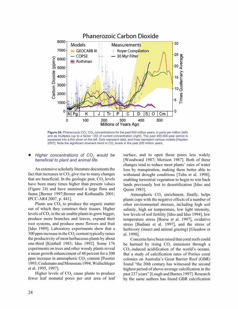
24

Figure 24: Phanerozoic CO2: CO2 concentrations for the past 600 million years, in parts per million (left)and as multiples (up to a factor ~20) of current concentration (right). The past 400,000-year period issqueezed into a thin sliver on the left. Dots represent data, and lines represent various models [Hayden2007]. Note the significant downard trend in CO2 levels in the past 200 million years.

! Higher concentrations of CO2 would bebeneficial to plant and animal life. An extensive scholarly literature documents the

fact that increases in CO2 give rise to many changesthat are beneficial. In the geologic past, CO2 levelshave been many times higher than present values(Figure 24) and have sustained a large flora andfauna [Berner 1997;Berner and Kothaualla 2001;IPCC-AR4 2007, p. 441].

Plants use CO2 to produce the organic matterout of which they construct their tissues. Higherlevels of CO2 in the air enable plants to grow bigger,produce more branches and leaves, expand theirroot systems, and produce more flowers and fruit[Idso 1989]. Laboratory experiments show that a300 ppm increase in the CO2 content typically raisesthe productivity of most herbaceous plants by aboutone-third [Kimball 1983; Idso 1992]. Some 176experiments on trees and other woody plants reveala mean growth enhancement of 48 percent for a 300ppm increase in atmospheric CO2 content [Poorter1993; Ceulemans and Mousseau 1994; Wullschlegeret al. 1995, 1997].

Higher levels of CO2 cause plants to producefewer leaf stomatal pores per unit area of leaf

surface, and to open those pores less widely[Woodward 1987; Morison 1987]. Both of thesechanges tend to reduce most plants’ rates of waterloss by transpiration, making them better able towithstand drought conditions [Tuba et al. 1998],enabling terrestrial vegetation to begin to win backlands previously lost to desertification [Idso andQuinn 1983].

Atmospheric CO2 enrichment, finally, helpsplants cope with the negative effects of a number ofother environmental stresses, including high soilsalinity, high air temperature, low light intensity,low levels of soil fertility [Idso and Idso 1994], lowtemperature stress [Boese et al. 1997], oxidativestress [Badiani et al. 1997], and the stress ofherbivory (insect and animal grazing) [Gleadow etal. 1998].

Concerns have been raised that coral reefs couldbe harmed by rising CO2 emissions through aCO2-induced acidification of the world’s oceans.But a study of calcification rates of Porites coralcolonies on Australia’s Great Barrier Reef (GBR)found “the 20th century has witnessed the secondhighest period of above-average calcification in thepast 237 years” [Lough and Barnes 1997]. Researchby the same authors has found GBR calcification

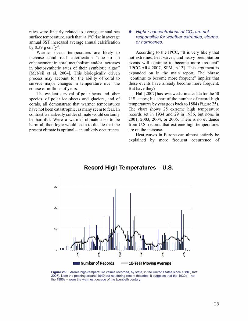
25

Figure 25: Extreme high-temperature values recorded, by state, in the United States since 1880 [Hart2007]. Note the peaking around 1940 but not during recent decades; it suggests that the 1930s – notthe 1990s – were the warmest decade of the twentieth century.

rates were linearly related to average annual seasurface temperature, such that “a 1ºC rise in averageannual SST increased average annual calcificationby 0.39 g cm-2y-1.”

Warmer ocean temperatures are likely toincrease coral reef calcification “due to anenhancement in coral metabolism and/or increasesin photosynthetic rates of their symbiotic algae”[McNeil et al. 2004]. This biologically drivenprocess may account for the ability of coral tosurvive major changes in temperature over thecourse of millions of years.

The evident survival of polar bears and otherspecies, of polar ice sheets and glaciers, and ofcorals, all demonstrate that warmer temperatureshave not been catastrophic, as many seem to fear. Incontrast, a markedly colder climate would certainlybe harmful. Were a warmer climate also to beharmful, then logic would seem to dictate that thepresent climate is optimal – an unlikely occurrence.

! Higher concentrations of CO2 are notresponsible for weather extremes, storms,or hurricanes.

According to the IPCC, “It is very likely thathot extremes, heat waves, and heavy precipitationevents will continue to become more frequent”[IPCC-AR4 2007, SPM, p.12]. This argument isexpanded on in the main report. The phrase“continue to become more frequent” implies thatthese events have already become more frequent.But have they?

Hall [2007] has reviewed climate data for the 50U.S. states; his chart of the number of record-hightemperatures by year goes back to 1884 (Figure 25).The chart shows 25 extreme high temperaturerecords set in 1934 and 29 in 1936, but none in2001, 2003, 2004, or 2005. There is no evidencefrom U.S. records that extreme high temperaturesare on the increase.

Heat waves in Europe can almost entirely beexplained by more frequent occurrence of

26

9. The Economic Effects of ModestWarming Are Likely to be Positive

circulation anomalies (more southerly flow). Therole of CO2 in causing those circulation anomaliesis poorly understood, making attribution impossibleat this time.

There has been an intense debate also whethera warmer climate will lead to more severe stormsand to more frequent and/or more intense tropicalcyclones. Regarding storms, claims that heavyprecipitation events in the U.S. increased between1900 and 1990 [Karl and Knight 1998] fails toprovide evidence that the increase has anything todo with greenhouse gases or temperature,particularly since there was a slight decline intemperatures during that period. Increases inmaximum annual 24-hour precipitation amountshave not been observed in Germany in the past 50years [DWD, German National Weather Service],the Iberian Peninsula [Gallego et al. 2006] or inparts of China [Wu et al. 2007].

It seems quite plausible that higher values ofSST would produce stronger hurricanes [Emanuel2005; Emanuel and Mann 2006]. But historicrecords of Atlantic hurricanes do not bear out sucha prediction [Goldenberg et al. 2001; Landsea 2005,2006, 2007]. Recent work by Vecchi and Soden[2007] suggests a warmer climate would lead toincreased vertical wind shear, which would impedethe development of tropical cyclones (hurricanes).And regarding mid-latitude storms, a globalwarming will lead to a lessening of temperaturegradients between the equator and the poles andtherefore to fewer and/or less intense storms[Legates 2004, Khandekar 2005].

Concern that anthropogenic global warmingmight result in harm to human health and welfareasserts connections between modest increases intemperature and increased morbidity and mortalitydue to heat stress, the spread of tropical diseasessuch as malaria and dengue fever, and the negativeeffects of warming on some industries. There islittle evidence to support these claims, andconsiderable evidence in support of the oppositeconclusion, that warmer temperatures benefit humanhealth and prosperity.

! Human health benefits from warmertemperatures.

In temperate regions, human mortality andmorbidity tend to show clear maxima in the winterand secondary maxima in the summer. While thesecondary maxima are more pronounced in regionswith warmer summer climates, as in the southernU.S. and southern Europe, even in those regions thesecondary maxima are smaller than the wintermaxima. A warming of even 3ºC in the next 100years would, on balance, be beneficial to humansbecause the reduction of wintertimemortality/morbidity would be several times largerthan the increase in summertime heat stress-relatedmortality/morbidity [Laaidi 2006, Keatinge 2000].

The claim that malaria would spread under awarmer climate has been severely critiqued by PaulReiter, professor, Institute Pasteur, Unit of Insectsand Infectious Diseases, Paris, France, who pointsout that the incidence of malaria depends on anumber of factors, few of them related to climate ortemperature. Historically, malaria was widespreadthroughout many areas in the temperate or evencolder regions of the mid-latitudes [Reiter 2005].

! Economic benefits from global warming

Beneficial economic effects of warmertemperatures include longer growing seasons intemperate climates, benefitting agriculture andforestry industries [Idso and Idso 2000], lowerheating bills, and lower construction costs.Mendelsohn and Neumann [1999] presented asynthesis of previous studies on the costs andbenefits of global warming, which is summarized inFigure 26.

Mendelsohn and Neumann assumed an increasein temperature of 2.5°C, a 7 percent increase inprecipitation, and an increase to 530 ppmatmospheric carbon dioxide by 2060, which theyadmit “may be somewhat more severe than the mostrecent scientific assessment in IPCC (1996a).” Theyfound the net impact of global warming on the U.S.economy in the year 2060, if no action were takento slow or stop emissions, would be positive, to thetune of $36.9 billion, or about 0.2 percent ofprojected GDP. In 2001 dollars this would be about$11.5 billion. The benefits of global warming to theagricultural and timber industries more than

27

Estimated Annual Impact on U.S. ofDoubling of CO2 (billions of 1990$)

Sector 2060 economy 1990 economy

Market sector impact estimates

Agriculture +$41.4 +$11.3

Timber +$3.4 +$3.4

Water resources -market only

- $3.7 -$3.7

Energy -$4.1 -$2.5

Coastal structures -$0.1 -$0.1

Commercialfishing

-$0.4 to +$0.4 -$0.4 to +$0.4

Total (marketsectors)

+$36.9(+0.2% of 2060GDP)

+$8.4(+0.2% of 1990GDP)

Nonmarket sector impact estimates

Water quality -$5.7 -$5.7

Recreation +$3.5 +$4.2

Figure 26. The net effects of the modest warming caused bya doubling of carbon dioxide concentrations are likely to bepositive in the U.S., with benefits exceeding costs by some$36.9 billion a year in 2060 (+0.2 percent of 2060 GDP.Adapted from Mendelsohn and Neumann 1999, Table 12.2,page 320.

10. Conclusion

outweigh losses to the energy industry or damage tocoastal structures.

Economist Thomas Gale Moore [1998]alsofound that earlier estimates exaggerated the costs ofwarming. Moore used historical data to calculatethat if temperatures were 4.5ºF warmer in the U.S.,41,000 fewer people would die each year fromrespiratory and circulation diseases. The annualbenefits of global warming to the U.S., he estimates,would exceed costs by $104.8 billion in 1990dollars.

The central problems for policymakers in the debateover global warming are (a) is the reported warmingtrend real and how significant is it? (b) how much ofthe warming trend is due to natural causes and howmuch is due to human-generated greenhouse gases?

and (c) would the effects of continued warming beharmful or beneficial to plant and wildlife and tohuman civilization?

In this NIPCC report we have presentedevidence that helps provide answers to all threequestions.

! The extent of the modern warming – the subjectof the first question – appears to be less than isclaimed by the IPCC and in the popular media.We have documented shortcomings of surfacedata affected by urban heat islands and by thepoor distribution of land-based observingstations. Data from oceans, covering 70 percentof the globe, are also subject to uncertainties.The only truly global observations come fromweather satellites, and these have not shownany warming trend since 1998, for the past 10years.

! This report shows conclusively that the humangreenhouse gas contribution to current warmingis insignificant. Our argument is based on thewell- established and generally agreed-to‘fingerprint’ method. Using data published bythe IPCC and further elaborated in theU.S.-sponsored CCSP report, we have shownthat observed temperature- trend patternsdisagree sharply with those calculated fromgreenhouse models.

It is significant that the IPCC has nevermade such a comparison, or it would havediscovered the same result – namely that thecurrent warming is primarily of natural originrather than anthropogenic. Instead, the IPCCrelied for its conclusion (on AGW) oncircumstantial ‘evidence’ that does not hold upunder scrutiny.

! We show that the twentieth century is in no wayunusual and that warming periods of greatermagnitude have occurred in the historic past –without any catastrophic consequences.

! We also discuss the many shortcomings ofclimate models in trying to simulate what ishappening in the real atmosphere.

! If the human contribution to global warmingdue to increased levels of greenhouse gases isinsignificant, why do greenhouse gas models

28

calculate large temperature increases, i.e., showhigh values of ‘climate sensitivity’? The mostlikely explanation is that models ignore thenegative feedbacks that occur in the realatmosphere. New observations reported fromsatellites suggest it is the distribution of watervapor that could produce such strong negativefeedbacks.

! If current warming is not due to increasinggreenhouse gases, what are the natural causesthat might be responsible for both warming andcooling episodes – as so amply demonstrated inthe historic, pre-industrial climate record?Empirical evidence suggests very strongly thatthe main cause of warming and cooling on adecadal scale derives from solar activity via itsmodulation of cosmic rays that in turn affectatmospheric cloudiness. According to publishedresearch, cosmic-ray variations are alsoresponsible for major climate changes observedin the paleo-record going back 500 millionyears.

! The third question concerns the effects ofmodest warming. A major scare associated witha putative future warming is a rapid rise in sealevel, but even the IPCC has been scaling backits estimates. We show here that there will belittle if any acceleration, and therefore noadditional increase in the rate of ongoing sea-level rise. This holds true even if there is adecades-long warming, whether natural ormanmade.

! Other effects of a putative increase intemperature and carbon dioxide are likely to bebenign, promoting not only the growth of cropsand forests but also benefiting human health.Ocean acidification is not judged to be aproblem, as indicated by available data. Afterall, CO2 levels have been up to 20 times thepresent value during the Phanerozoic Period,the past 500 million years. During this timeEarth’s climate has been remarkably stable,with no ‘run-away’ greenhouse effects –indicating strong negative feedbacks.

! If, for whatever reason, a modest warming wereto occur – even one that matches temperatures

seen during the Medieval Warm Period ofaround 1100 AD or the much larger onesrecorded during the Holocene ClimateOptimum of some 6,000 years ago – the impactwould not be damaging but would probably be,on the whole, beneficial. [Lamb 1982, andFigure 26]

! Policy Implications

! Our findings, if sustained, point to naturalcauses and a moderate warming trend withbeneficial effects for humanity and wildlife.This has obvious policy implications: Schemesproposed for controlling CO2 emissions,including the Kyoto Protocol, proposals in theU.S. for federal and state actions, and proposalsfor a successor international treaty to Kyoto, areunnecessary, would be ineffective ifimplemented, and would waste resources thatcan better be applied to genuine societalproblems [Singer, Revelle and Starr 1991;Lomborg 2007].

! Even if a substantial part of global warmingwere due to greenhouse gases – and it is not –any control efforts currently contemplatedwould give only feeble results. For example, theKyoto Protocol – even if punctiliously observedby all participating nations – would decreasecalculated future temperatures by only 0.02degrees C by 2050 [re-calculated from Parry etal. 1998], an undetectable amount.

To sum up: This NIPCC report falsifies theprincipal IPCC conclusion that the reportedwarming (since 1979) is very likely caused by thehuman emission of greenhouse gases. In otherwords, increasing carbon dioxide is notresponsible for current warming. Policiesadopted and called for in the name of ‘fightingglobal warming’ are unnecessary.

It is regrettable that the public debate overclimate change, fueled by the errors andexaggerations contained in the reports of the IPCC,has strayed so far from scientific truth. It is anembarrassment to science that hype has replacedreason in the global debate over so important anissue.

About the Contributors

Anderson, Warren. Economist, George MasonUniversity, author of Fire and Ice. Fairfax,Virginia, USA

Avery, Dennis. Director, Center for Global FoodIssues, co-author of Unstoppable GlobalWarming. USA

Battaglia, Franco. Professor of Chemical Physicsand Environmental Chemistry, University ofModena. Italy

Carter, Bob. Paleoclimatologist and professor,James Cook University. Townsville, Australia

Courtney, Richard. Engineering expert for fuel useand climate consequences. United Kingdom

D’Aleo, Joseph. Meteorologist, fellow and electedcouncilor AMS; first director of meteorology, TheWeather Channel. USA

Goldberg, Fred, Ph.D. (Technology) polar expert,and co-organizer of 2006 Stockholm ClimateConference. Sweden

Gray, Vincent, Ph.D. (Chemistry) and publisher ofNew Zealand Climate Newsletter. New Zealand

Haapala, Kenneth. Economist, energy andeconomic modeler. USA

Heiss, Klaus, Ph.D. Economist and author ofsurvey studies of climate. Austria

Idso, Craig, Ph.D. (Ag Meteorology), andpublisher of CO2Science.org. Tempe, Arizona,USA

Jaworowski, Zbigniew. Professor, CentralLaboratory for Radiological Protection. Warsaw,Poland

Kärner, Olavi, Ph.D. (Physics), Tartu Observatory.Estonia

Khandekar, Madhav, Ph.D. Meteorologist,formerly with Environment Canada. ExpertReviewer, IPCC 2007. Ontario, Canada

Kininmonth, William. Meteorologist, former headof National Climate Centre, Australian Bureau ofMeteorology. Australia

Labohm, Hans. Economist, former deputy foreignpolicy planning advisor, Netherlands Ministry ofForeign Affairs. Netherlands

Monckton, Christopher. Climate analyst, formeradvisor to Prime Minister Margaret Thatcher.Scotland.

Motl, Lubos, Ph.D. (Physics), former fellow atHarvard, publisher of The Reference Frame blog.Czech Republic

Segalstad, Tom V. Associate Professor and headof Geological Museum, University of Oslo.Norway

Singer, Fred. Atmospheric physicist and formerdirector of U.S. Weather Satellite Service. USA.

Taylor, George. Oregon State University, formerpresident of Association of State Climatologists.USA

Thoenes, Dick. Professor Emeritus, EindhovenUniversity and co-author Man-Made GlobalWarming: Unravelling a Dogma. Netherlands

Uriarte, Anton. Professor of Climatology andGeography, Universidad del Pais Vasco. Spain

Weber, Gerd-Rainer, Ph.D. (University ofIndiana), Consulting meteorologist. Germany

30

About the Editor

S. Fred Singer, an atmospheric and space physicist, is founder and president of the Science andEnvironmental Policy Project, a nonprofit research and education organization based in Arlington, Virginia.He is professor emeritus of environmental sciences at the University of Virginia.

Singer is the author or coauthor of many books and scholarly articles. Recently he coauthored, withDennis Avery, Unstoppable Global Warming – Every 1,500 Years (Rowman & Littlefield, 2007), which wason the New York Times bestsellers list. Singer’s previous books include The Greenhouse Debate Continued:An Analysis and Critique of the IPCC Climate Assessment (ICS Press, 1992), Climate Policy – From Rio toKyoto (Hoover Institution, 2000), and Hot Talk Cold Science – Global Warming’s Unfinished Debate(Independent Institute, 1997, 1999).

Singer has been a pioneer in many ways. At the Applied Physics Laboratory of Johns Hopkins University,he participated in the first experiments using high-altitude research rockets, measuring the energy spectrumof primary cosmic rays and the distribution of stratospheric ozone; he is generally credited with the discoveryof the equatorial electrojet current flowing in the ionosphere. In academic science during the 1950s, hepublished the first studies on subatomic particles trapped in the Earth’s magnetic field – radiation belts, laterdiscovered by James Van Allen. He was the first to make the correct calculations for using atomic clocks inorbit, contributing to the verification of Einstein’s General Theory of Relativity, and now essential in the GPSsystem of satellite navigation. He also designed satellites and instrumentation for remote sensing of theatmosphere and received a White House Presidential Commendation for this work.

In 1971 he calculated the anthropogenic contribution to atmospheric methane, an important greenhousegas. He also predicted that methane, once reaching the stratosphere, would transform into water vapor, whichcould then deplete stratospheric ozone. A few years later, methane levels were indeed found to be rising, andthe increase in stratospheric water vapor was confirmed in 1995.

Singer has served as chief scientist, U.S. Department of Transportation (1987- 89); deputy assistantadministrator for policy, U.S. Environmental Protection Agency (1970-71); deputy assistant secretary forwater quality and research, U.S. Department of the Interior (1967- 70); founding dean of the School ofEnvironmental and Planetary Sciences, University of Miami (1964-67); first director of the National WeatherSatellite Service (1962-64); and director of the Center for Atmospheric and Space Physics, University ofMaryland (1953-62).

In the 1980s, Singer served for five years as vice chairman of the National Advisory Committee forOceans and Atmosphere (NACOA). He currently directs the nonprofit Science and Environmental PolicyProject, which he founded in 1990 and incorporated in 1992 after retiring from the University of Virginia.

For more information, visit the Web site of the Science and Environmental Policy Project atwww.sepp.org.

31

References

Anonymous 1994. IPCC’s ritual on global warming. Nature371: 269.

Badiani, M., Paolacci, A.R., D’Annibale, A., Miglietta, F., andRaschi, A. 1997. Can rising CO2 alleviate oxidative risk for theplant cell? Testing the hypothesis under natural CO2enrichment. In: Raschi, A., Miglietta, F., Tognetti, R., and vanGardingen, P.R., Eds. Plant Responses to Elevated CO2:Evidence from Natural Springs. Cambridge University Press,Cambridge, United Kingdom, pp. 221-241.

Baker, D.F. 2007. Reassessing carbon sinks. Science 316:1708-1709. DOI10.1126/science.1144863.

Baliunas, S., and R. Jastrow 1990. Evidence for long-termbrightness changes of solar-type stars. Nature 348: 520-522.

Beck, E-G. 2007. 180 years of atmospheric CO2 gas analysis bychemical methods. Energy & Environment 18(2). http://www.biokurs.de/treibhaus/180CO2_supp.htm

Berner, R.A. 1997. The rise of plants and their effect onweathering and atmospheric CO2. Science 276: 544-545.

Berner, R.A., and Z. Kothavala 2001. GEOCARB III: Arevised model of atmospheric CO2 over phanerozoic time.Am. J. Sci. 301(2): 182-204.

Bindschadler, R. 1998. Future of the West Antarctic icesheet. Science 282: 428-429.

Boehm F., et al. 2002. Evidence for preindustrial variationsin the marine surface water carbonate system from corallinesponges. Geochem., Geophys., Geosystems, Research Letter3. DOI:10.1029/2001GC000264.

Boese, S.R., Wolfe, D.W., and Melkonian, J.J. 1997.Elevated CO2 mitigates chilling-induced water stress andphotosynthetic reduction during chilling. Plant Cell Environ.20: 625-632.

Castles, I., and D. Henderson 2003. The IPCC emissionscenarios: An economic-statistical critique. Energy &Environment 14 (2-3): 159-185.

Cazenave, A., and R.S. Nerem 2004. Present-day sea levelchange: Observations and causes. Rev. Geophys., 42.RG3001. DOI:10.1029/2003RG000139.

Cess, R.D., G.L. Potter, et al. 1990. Intercomparison andinterpretation of climate feedback processes in nineteenatmospheric general circulation models. Journal ofGeophysical Research 95(16): 601-616, 615.

Cess, R.D., G.L. Potter, et al. 1996. Cloud feedback inatmospheric general circulation models. Journal ofGeophysical Research 101(12): 791-812, 794.

Ceulemans, R. and Mousseau M. 1994. Effects of elevated

CO2 on woody plants. New Phytologist 127: 425-446.

Conway, H. et al. 1999. Past and future grounding-lineretreat of the WAIS. Science 286: 280-288.

Dahl-Jensen, D. et al. 1999. Past temperature directly fromthe Greenland Ice Sheet. Science 282: 268-271.

Dlugokencky, E.J., K.A. Masarie, P.M. Lang, and P.P. Tans1998. Continuing decline in the growth rate of theatmospheric methane burden. Nature 393: 447-450.

Doney, S.C., 2006. The Dangers of Ocean Acidification.Scientific American 294: 58-65.

Douglas, B., M. Kearney, S. Leatherman (eds) 2001. SeaLevel Rise History and Consequences. Academic Press.

Douglas, B.C. and W.R. Peltier 2002. The puzzle of globalsea-level rise. Physics Today, March.

Douglass, D.H., B. Pearson, S.F. Singer 2004. Altitudedependence of atmospheric temperature trends: Climatemodels versus observations. Geophys. Res. Letters 31.

Douglass, D.H., J.R. Christy, B.D. Pearson, and S.F. Singer2007. A comparison of tropical temperature trends withmodel predictions. Intl J Climatology (Royal Meteorol Soc).DOI:10.1002/joc.1651.

DWD, German National Weather Service DWD (GermanWeather Service). Klimatologische Werte fur das Jahr(Annual climate data.) Offenbach, Germany

Ellsaesser, H.W. 1984. The climate effect of CO2.Atmospheric Environment 18: 431-434.

Emanuel, K. 2005. Increasing destructiveness of tropicalcyclones over the past 30 years. Nature 436: 686-688.

Emanuel, K.A. and M.E. Mann 2006. Atlantic hurricanetrends linked to climate change. Eos 87: 233-241.

Fairbanks, R.G. 1989. A 17,000 year glacio-eustatic sea levelrecord: Influence of glacial melting rates on the YoungerDryas event and deep-ocean circulation. Paleoceanography342: 637-642.

Fan, S., et al. 1998. A large terrestrial carbon sink in NorthAmerica implied by atmospheric and oceanic carbon dioxidedata and models. Science 282: 442-446.

Fine, M. and D. Tchernov 2007. Scleractinian coral speciessurvive and recover from decalcification. Science 315: 1811.

Fischer, H., et al. 1999. Carbon dioxide in the Vostok icecore. Science 283: 1712-1714.

Friis-Christensen, E. and K. Lassen 1991. Length of the solarcycle: An indicator solar activity closely associated with

32

climate. Science 254: 698-700.

Gallego et al, 2006. Change in frequency and intensity ofdaily precipitation over the Iberian Peninsula. J. Geoph. Res.111, D24105, doi: 10.1029/2006JD0077280.

Gleadow, R.M., Foley, W.J. and Woodrow, I.E. 1998.Enhanced CO2 alters the relationship betweenphotosynthesis and defense in cyanogenic Eucalyptuscladocalyx F. Muell. Plant Cell Environ. 21: 12-22.

Goldenberg, S.B., C.W. Landsea, A.M. Mestas-Nunez, andW.M. Gray 2001. The recent increase in Atlantic hurricaneactivity: Causes and implications. Science 293: 474-479.

Goodrich, J.D. 1996. Comments on Regional Simulations ofGreenhouse Warming Including Natural Variability. Bulletinof the American Meteorological Society 77:3-4 (July).

Gouretski, V. and K.P. Koltermann 2007. How much is theocean really warming? Geophysical Research Letters 34L01610.

Haigh, J.D. 1996: The impact of solar variability on climate.Science 272: 981-985.

Haigh, J.D. 2003. The effects of solar variability on theEarth’s climate. Philos. Trans. R. Soc. London Ser. A 361:95-111.

Hall, B. 2007. http://hallofrecord.blogspot.com/2007/02/extreme-temperatures-wheres-global.html.

Hansen, J.E. 2006. The threat to the planet. New YorkReview of Books 53, July 13, 2006.

Hansen, J.E., et al. 1998. Climate forcings in the industrialera. Proc. Natl. Acad. Sci. USA 95: 12753-12758.

Hansen, J.E., et al. 2005. Earth’s energy imbalance:Confirmations and implications. Science 308 (5727):1431-1435.

Hayden, H. 2007. Private communication.

Held, I.M., and B.J. Soden 2006. Robust responses of thehydrological cycle to global warming. J. Clim. 19: 5686-5699.

Henderson, D. 2005. SRES, IPCC, and the Treatment ofEconomic Issues: What Has Emerged. Energy andEnvironment 16 (3 & 4).

Holgate, S.J. 2006. On the decadal rates of sea-level changeduring the twentieth century. Geophys Res Lett 34. DOI:10.1029/2006GL028492,2007.

Idso, C.D. and Idso, K.E. 2000. Forecasting world foodsupplies: The impact of the rising atmospheric CO2concentration. Technology 7S: 33-56.

Idso, K.E. 1992. Plant responses to rising levels of carbondioxide: A compilation and analysis of the results of adecade of international research into the direct biological

effects of atmospheric CO2 enrichment. ClimatologicalPublications Scientific Paper #23, Office of Climatology,Arizona State University, Tempe, AZ.

Idso, K.E. and Idso, S.B. 1994. Plant responses toatmospheric CO2 enrichment in the face of environmentalconstraints: A review of the past 10 years’ research.Agricultural and Forest Meteorology 69: 153-203.

Idso, S.B. 1989. Carbon Dioxide: Friend or Foe? IBR Press,Tempe, AZ.

Idso, S.B., and Quinn, J.A. 1983. Vegetational Redistributionin Arizona and New Mexico in Response to a Doubling ofthe Atmospheric CO2 Concentration. Laboratory ofClimatology, Arizona State University, Tempe, Arizona.

Information Quality Act 2004. www.it.ojp.gov/documents/crs_iq_act_omb_guidance_and_implementation.pdf.

IPCC 2008. “About IPCC,” http://www.ipcc.ch/about/index.htm, accessed 2/15/08.

IPCC-AR4 2007. Climate Change 2007: The PhysicalScience Basis. Contribution of Working Group I to theFourth Assessment Report of the Intergovernmental Panel onClimate Change. Cambridge University Press.

IPCC-FAR 1990. Scientific Assessment of Climate Change.Contribution of Working Group I to the First AssessmentReport of the Intergovernmental Panel on Climate Change.Cambridge University Press.

IPCC-SAR 1996. Climate Change 1995: The Science ofClimate Change. Contribution of Working Group I to theSecond Assessment Report of the Intergovernmental Panelon Climate Change, Cambridge University Press.

IPCC-TAR 2001. Climate Change 2001: The ScientificBasis. Contribution of Working Group I to the ThirdAssessment Report of the Intergovernmental Panel onClimate Change. Cambridge University Press.

Jaworowski, Z. 1994. Ancient atmosphere - validity of icerecords. Environmental Science & Pollution Research 1(3):161-171.

Jaworowski Z., Segalstad T.V., and Ono N. 1992. Doglaciers tell a true atmospheric CO2 story? The Science of theTotal Environment 114: 227-284.

Karl, T.R., S.J. Hassol, C.D. Miller, and W.L. Murray (eds.)2006. Temperature Trends in the Lower Atmosphere: Stepsfor Understanding and Reconciling Differences. A report bythe Climate Change Science Program and Subcommittee onGlobal Change Research, http://www.climatescience.gov/Library/sap/sap1-1/finalreport/default.htm.

Karl and Knight, 1998. Secular trend of precipitationamount, frequency and intensity in the United States. Bull.Am. Met. Soc. 79: 231 - 242.

33

Keatinge W.R. et al, 2000. Heat related mortality in warmand cold regions of Europe: Observational study. Brit. Med.Journal 321: 670 - 673.

Keeling, R.F., S.C. Piper, and M. Heimann 1996. Global andhemispheric CO2 sinks deduced from changes in atmosphericO2 concentration. Nature 381: 218-221.

Keeling, R.F. and S.R. Shertz 1992: Seasonal and interannualvariations in atmospheric oxygen and implications for theglobal carbon cycle. Nature 358: 723-727.

Keigwin, L.D. 1996. The Little Ice Age and Medieval WarmPeriod in the Sargasso Sea. Science 274: 1504-1508.

Kerr, R.A. 2007. Humans and nature duel over the nextdecade’s climate. Science 317: 746-747.

Khandekar M.L. 2005. Extreme weather trends vs dangerousclimate change: A need for a critical reassessment. Energy &Environment 16: 327-331.

Kiehl, J.T. 2007. Twentieth century climate model responseand climate sensitivity. Geophys Res Lett 34: L22710.DOI:10.1029/2007GL031383.

Kimball, B.A. 1983. Carbon dioxide and agricultural yield:An assemblage and analysis of 770 prior observations. U.S.Water Conservation Laboratory, Phoenix, AZ.

Knight, C.G., et al. 2007. Association of parameter, software,and hardware variation with large-scale behavior across57,000 climate models. PNAS 104: 12259-12264.DOI:10.1073/ pnas.0608144104.

Kriplani, R.H., A. Kulkarni, S.S. Sabde, and M.L. Khandekar2003. Indian Monsoon variability in a global warmingscenario. Natural Hazards 29: 189-206.

Laaidi, M. et al, 2006. Temperature related mortality inFrance, a comparison between regions with different climatesfrom the perspective of global warming. Int. J.Biometeorology, 51: 145 - 153.

Lamb, Hubert H. 1982, 1995. Climate, History and theModern World. Rutledge, New York, NY.

Landsea, C.W. 2005. Hurricanes and global warming:Arising from Emanuel 2005a. Nature 438: E11-E13.DOI:10.1038/ nature04477.

Landsea, C.W. 2007. Counting Atlantic tropical cyclonesback to 1900. Eos 88: 197-202.DOI:10.1029/2007EO180001.

Landsea, C.W., et al. 2006. Can we detect trends in extremetropical cyclones? Science 313: 452-454. DOI:10.1126/science.1128448.

Le Quere, C. et al. 2007. Saturation of the Southern OceanCO2 sink due to recent climate change. Science 316:1735-1738. DOI:10.1126/science.1136188.

Lean, J, J. Beer, and R. Bradley 1995. Reconstruction ofsolar irradiance since 1610: Implications for climate change.Geophys. Res. Lett 22: 3195-3198.

Legates, D.R. 2004. Global Warming and the HydrologicCycle: How Are the Occurrence of Floods, Droughts, andStorms Likely to Change? George Marshall Institute,Washington, D.C.

Lindzen, R.S. 1990. Some coolness concerning globalwarming. Bulletin of the American Meteorological Society71: 288-299.

Lo, J., Z. Yang, and R. A. Pielke (2008). Assessment of threedynamical climate downscaling methods using the WeatherResearch and Forecasting (WRF) model. J. Geophys. Res.,doi:10.1029/2007JD009216, in press.

Lockwood, M. and C. Fröhlich. 2007. Recent oppositelydirected trends in solar climate forcings and the global meansurface air temperature. Proc. Royal Soc. A. 463: 2447-60.

Loehle, C., 2007: A 2000-year global temperaturereconstruction based on non-tree-ring proxies. Energy andEnvironment 18: 1049-1058.

Loehle, Craig and J.H. McCulloch. 2008. Correction to: A2000-year global temperature reconstruction based onnon-tree ring proxies. Energy and Environment (in press).

Lomborg, Bjørn. 2007. Cool It: The SkepticalEnvironmentalist's Guide to Global Warming. Knopf.

Lough, J.M. and Barnes, D.J. 1997. Several centuries ofvariation in skeletal extension, density and calcification inmassive Porites colonies from the Great Barrier Reef: Aproxy for seawater temperature and a background ofvariability against which to identify unnatural change.Journal of Experimental and Marine Biology and Ecology211: 29-67.

Lucarini, V., S. Calmanti, A. Dell’Aquila, P.M. Ruti, and A.Speranza 2007. Intercomparison of the northern hemispherewinter mid-latitude atmospheric variability of theIPCC models. Climate Dynamics 28: 829-848.

Lyman, J.M., et al. 2006. Recent cooling of the upper ocean.Geophys. Res. Lett. 33: L18604.DOI:10.1029/2006GL027033.

Maddox J. 1991. Making global warming public property.Nature 349: 189.

Mantua, N.J., et al. 1997. A Pacific interdecadal climateoscillation with impacts on salmon production. Bull. Am.Meteorol. Soc. 78: 1069-1079.

Marchitto, et al. 2005. Deep Pacific CaCO3 compensationand glacial-interglacial atmospheric CO2. Earth andPlanetary Science Letters 231(3-4): 317-336.

Marland, G., T.A. Boden, and R. J. Andres. 2007. Global,Regional, and National CO2 Emissions. In Trends: A

34

Compendium of Data on Global Change. Carbon DioxideInformation Analysis Center, Oak Ridge NationalLaboratory, U.S. Department of Energy, Oak Ridge,Tennessee, U.S.A.

McIntyre, S. 2007. IPCC and Data Access. http://www.climateaudit.org/?p=640.

McIntyre, S. and R. McKitrick 2003. Corrections to Mann etal. (1998) proxy data base and northern hemisphere averagetemperature series. Energy & Environment 14: 751-777.

McIntyre, S. and R. McKitrick 2005. Hockey sticks,principal components and spurious significance. GeophysicalResearch Letters 32 L03710.

McKitrick, R. et al. 2007. Independent Summary forPolicymakers IPCC Fourth Assessment Report. FraserInstitute.

McKitrick, R. and P.J. Michaels 2004. A test of correctionsfor extraneous signals in gridded surface temperature data.Clim Res 26: 159-173.

McKitrick, R. and P.J. Michaels 2008. Quantifying theinfluence of anthropogenic surface processes andinhomogeneities on gridded global climate data. Journal ofGeophysical Research (in press).

McNeil, B.I., Matear, R.J. and Barnes, D.J. 2004. Coral reefcalcification and climate change: The effect of oceanwarming. Geophysical Research Letters 31:10.1029/2004GL021541.

Mendelsohn R. and J.E. Neumann (eds.) 1994. The Impact ofClimate Change on the United States Economy. CambridgeUniversity Press, Cambridge.

Met Office 2007. The forecast for 2014, news release. U.K.Met Office, August 10, 2007.

Michaels, P.J. and P.C. Knappenberger 1996. Human effecton global climate? Nature 384: 522-523.

Minnett, P. 2006. Why greenhouse gases heat the ocean.Sept. 5, 2006.http://www.realclimate.org/index.php/archives/2006/09/why-greenhouse-gases-heat-the-ocean/.

Moore, T. G. 1995. Global Warming: A Boon to Humansand Other Animals. Hoover Institution, Stanford University,Stanford CA.

Moore, T.G. 1998. Climate of Fear: Why We Shouldn’tWorry about Global Warming. Cato Institute.

Morison, J.I.L. 1987. Intercellular CO2 concentration andstomatal responses to CO2. In: Zeiger, E., Farquhar, G.D.,and Cowan, I.R., Eds. Stomatal Function. StanfordUniversity Press, Stanford, California, pp. 229-251.

Mörner, N.A. 2004. Estimating future sea level changes frompast records. Global and Planetary Change 40 (1-2): 49-54.

Mörner, N.A., M. Tooley, and G. Possnert 2004. Newperspectives for the future of the Maldives. Global andPlanetary Change 40: 177-182.

Munk, W. 2002. Twentieth-century sea level: An enigma.Proc. Natl. Acad. Sci. U.S.A. 99: 6550-6555.

Murphy, J.M., et al. 2004. Quantification of modellinguncertainties in a large ensemble of climate changesimulations. Nature 429: 768-772.

National Assessment for Climate Change (NACC) 2000.Climate Change Impacts on the United States. The PotentialConsequences of Climate Variability and Change. Availableat http://www.usgcrp.gov/usgcrp/Library/nationalassessment/overview.htm.

NAS 2000. Reconciling Observations of Global TemperatureChange. National Academy Press, Washington DC.

NAS 2006. Surface Temperature Reconstructions for theLast 2,000 Years. National Academy Press, Washington DC.

Neff, U., et al. 2001. Strong coherence between solarvariability and the monsoon in Oman between 9 and 6 kyrago. Nature 411: 290-293.

Oppenheimer, et al. 2007. The limits of consensus. Science317(5844): 1505-1506.

Parry et al. 1998. Adapting to the inevitable. Nature 395:741.

Paynter, D.J., I.V. Ptashnik, K.P. Shine, and K.M. Smith2007. Pure water vapor continuum measurements between3100 and 4400 cm-1: Evidence for water dimer absorption innear atmospheric conditions. Geophys. Res. Lett. 34 DOI:10.1029/2007GL029259.

Peterson, T.C. and R.S. Vose 1997. An Overview of theGlobal Historical Climatology Network TemperatureDatabase. Bulletin of the American Meteorological Society2837-2849.

Petit, J.R., J. Jouzel, et al. 1999. Climate and atmospherichistory of the past 420,000 years from the Vostok ice core inAntarctica. Nature 399: 429-436.

Pew 2007. Global Warming: A Divide on Causes andSolutions, Pew Research Center for the People and the Press,January 24, 2007, http://pewresearch.org/pubs/282/global-warming-a-divide-on-causes-and-solutions.

Poorter, H. 1993. Interspecific variation in the growthresponse of plants to an elevated ambient CO2 concentration.Vegetatio 104/105: 77-97.

Priestley, C.H.B. 1996. The limitation of temperature byevaporation in hot climates. Agricultural Meteorology(Elsevier) 3: 241-246.

Rahmstorf, S. 2007. A semi-empirical approach to projectingfuture sea-level rise. Science 315: 368-370.

35

Rahmstorf, S., et al. 2007. Recent climate observationscompared to projections. Science 316(5825): 709.

Reiter, P., 2005. The IPCC and technical information.Example: Impacts on human health.http://www.publications.parliament.uk/pa/ld200506/ldselect/ldeconaf/12/12we21.htm

Robinson, A.B., N.E. Robinson, and W. Soon 2007.Environmental effects of increased atmospheric carbondioxide. Journal of American Physicians and Surgeons 12:79-90.

Robock, A., et al. 2007. Climatic consequences of regionalnuclear conflicts. Atm. Chem. Phys. 7: 2003-2012.

Santer, B.D., et al. 1996. Towards the detection andattribution of an anthropogenic effect on climate. Clim. Dyn.12: 79-100.

Santer, B.D. and 23 coauthors 2005. Amplification of surfacetemperature trends and variability in the tropical atmosphere.Science 309: 1551-1555.

Scafetta, Nicola and B.J. West 2007. Phenomenologicalreconstructions of the solar signature in the NorthernHemisphere surface temperature records since 1600. Journalof Geophysical Research, 112, D24S03,doi:10.1029/2007JD008437.

Schlesinger, M.E. and N. Ramankutty 1994. An oscillation inthe global climate system of period 65-70 years. Nature 367:723-726.

Schwartz, S.E, 2007. Heat capacity, time constant, andsensitivity of Earth’s climate system. J. of Geophys. Res.DOI:10.1029/2007JD008746.

Schwartz, S.E., R.J. Charlson, and H. Rodhe 2007.Quantifying climate change - too rosy a picture? Nature 2:23-24.

Seitz, F. 1996. A Major Deception on Global Warming. TheWall Street Journal, June 12.

Senior, C.A. and J.F.B. Mitchell 1993. Carbon dioxide andclimate: The impact of cloud parameterization. J. Clim. 6:393-418.

SEPP 1992. The Greenhouse Debate Continued: An Analysisand Critique of the IPCC Climate Assessment. ICS Press,San Francisco, CA.

SEPP 1997. The Scientific Case Against the Global ClimateTreaty. www.sepp.org/publications/ GWbooklet/GW.html[Also available in German, French, and Spanish].

SEPP 2002. The Kyoto Protocol is Not Backed by Science.Science and Environmental Policy Project, Arlington VA.

Shaviv, N. J.. 2002. Cosmic ray diffusion from the galacticspiral arms, iron meteorites, and a possible climaticconnection? Phys. Rev. Lett. 89, 051,102.

Shaviv, N.J. 2005. On climate response to changes in thecosmic ray flux and radiative budget. J. Geophys. Res. 110:A08105.

Shaviv, N. J. and J. Veizer. 2003. A celestial driver ofphanerozoic climate? GSA Today, 13, 4-11.

Shindell, D.T. 2001. Climate and ozone response toincreased stratospheric water vapor. Geophys. Res. Lett. 28:1551-1554.

Shukla, J. 2007. Monsoon mysteries. Science 318: 204-205.

Singer, S.F. 1958. Cosmic-ray time variations produced bydeceleration in interplanetary space. Nuovo Cimento 8,Supple. II: 334-341.

Singer, S. F. 1971. Stratospheric water vapour increase dueto human activities. Nature 233: 543-547.

Singer, S. F. 1997, 1999. Hot Talk Cold Science. TheIndependent Institute, Oakland CA.

Singer, S. F. 1999. Human contribution to climate changeremains questionable. Also, Reply. Eos [Transaction AGU],80, 33, 186-187 and 372-373.

Singer, S. F. 2000. Climate policy – From Rio to Kyoto apolitical issue for 2000 and beyond. Essays in Public Policy102. Hoover Institution, Stanford University, Stanford CA.

Singer, S. F. 2001. Disparity of temperature trends ofatmosphere and surface. Paper presented at 12th Symposiumon Global Climate Change, Amer. Meteorol. Soc.,Albuquerque NM.

Singer S. F. 2005a. Are sea surface temperature (SST) trendsreal. Abstract for the AGU Joint Assembly, May 25, 2005,New Orleans LA.

Singer S. F. 2005b. A closer look at sea surface temperaturetrends: How effective is greenhouse (GH) warming of SST?Presentation at CCSP Workshop, November 14, 2005.http://www.climatescience.gov/workshop2005/posters/P-GC2.9_Singer.S.pdf.

Singer, S. F. 2006. How effective is greenhouse warming ofsea surface temperatures? In A. Zichichi and R. Ragini(eds.). International Seminar on Nuclear War and PlanetaryEmergencies. Climatology: Global Warming. WorldScientific Publishing Company, Singapore. pp. 176-182.

Singer, S.F. et al. 1997. Comments on ‘Open Letter to BenSanter.’ Bull Am Meteorolol Soc. 78: 81-82.

Singer, S. F., R. Revelle and C. Starr 1991. What to do aboutGlobal Warming: Look Before You Leap. Cosmos 1:28-33.

Singer, S. F. and D. Avery 2007. Unstoppable GlobalWarming: Every 1,500 Years. Rowman & LittlefieldPublishers, Inc.

Smith, D.M., et al., 2007. Improved surface temperature

36

prediction for the coming decade from a global climatemodel. Science 317: 796-799.

Soon, W.H. 2005. Variable solar irradiance as a plausibleagent for multidecadal variations in the Arctic-wide surfaceair temperature record for the past 130 years. Geophys. Res.Lett. 32 L16712.

Spencer, R.W., W.D. Braswell, J.R. Christy, and J. Hnilo2007. Cloud and radiation budget changes associated withtropical intraseasonal oscillations. Geophys. Res. Lett. 34L15707. DOI:10.1029/2007GL029698.

Stainforth, D.A., et al. 2005. Uncertainty in predictions of theclimate response to rising levels of greenhouse gases. Nature433: 403-406.

Stanhill, G. 2007. A perspective on global warming,dimming, and brightening. EOS, Transactions, AmericanGeophysical Union 88: 58.

Stephens, B.B., et al. 2007. Weak northern and strongtropical land carbon uptake from vertical profiles ofatmospheric CO2. Science 22(316): 1732-1735.DOI:10.1126/science.1137004.

Svensmark, H. 2007. Cosmoclimatology: a new theoryemerges. Astronomy & Geophysics 48: 1.18-1.24.

Svensmark, H., et al. 2007: Experimental evidence for therole of ions in particle nucleation under atmosphericconditions. Proc. Roy. Soc. A 463: 385-396.

Toscano, M.A. and I.G. Macintyre 2003. Corrected WesternAtlantic Sea Level Curve for last 11,000 years. Coral Reefs22: 257-270.

Trenberth, K. 2007. Prediction of climate. Nature webloghttp://blogs.nature.com/climatefeedback/2007/06/predictions_of_climate.html.

Trupin, A. and J. Wahr, 1990. Spectroscopic analysis ofglobal tide gauge sea level data. Geophysical JournalInternational 100: 441-453.

Tsonis A.A. and J.B. Elsner 1999. The autocorrelationfunction and human influences on climate. Technicalcomment and response by Wigley et al. Science 258.www.sciencemag.org/cgi/content/full/285/5427/495a.

Tsonis, A.A., K Swanson, and S Kravtsov 2007. A newdynamical mechanism for major climate shifts. GeophysicalResearch Letters V 34 L13705.

Tuba, Z., Csintalan, Z., Szente, K., Nagy, Z. and Grace, J.1998. Carbon gains by desiccation-tolerant plants at elevatedCO2. Functional Ecology 12: 39-44.

Usoskin, I.G. and G.A. Kovaltsov. 2007. Cosmic rays andclimate of the Earth: possible connection, C. R. GeoscienceDOI:10.1016/j.crte.2007.11.001.

Vecchi, G. A., and B. J. Soden 2007a. Increased tropical

Atlantic wind shear in model projections of global warming.Geophys. Res. Lett. 34 L08702.DOI:10.1029/2006GL028905.

Vecchi, G.A. and B.J. Soden 2007b. Global warming and thetropical weakening circulation. Journal of Climate 20(17):4316-4340.

Wegman, E., D.W. Scott, and Y. Said 2006. Ad HocCommittee Report to Chairman of the House Committee onEnergy & Commerce and to the Chairman of the Housesub-committee on Oversight & Investigations on theHockey-stick Global Climate Reconstructions. US House ofRepresentatives, Washington DC. Available athttp://energycommerce.house.gov/108/home/07142006Wegman Report.pdf.

Wentz, F.J., L. Ricciardulli, K. Hillburn, and C. Mears 2007.et al. 2007. How much more rain will global warming bring?Science 317: 233-235.

Wigley, T.M.L., R.L. Smith, and B.D. Santer 1998.Anthropogenic influence on the autocorrelation structure ofhemispheric-mean temperatures. Science 282: 1676-1679.

Wild, M. 2005. Solar radiation budgets in atmospheric modelintercomparisons from a surface perspective. Geophys. Res.Lett. 32. DOI:10.1029/2005GL022421.

Wild, M., et al. 2005. From dimming to brightening: Decadalchanges in solar radiation at earth’s surface. Science 308:847-850.

Willis, J.K., et al. 2007. Correction to “Recent cooling of theupper ocean.” Geophysical Research Letters 34: 16. DOI10.1029/2007GL030323.

Willson, R.C. and A.V. Mordvinov 2003. Secular totalirradiance trend during solar cycles 21-23. Geophys. Res.Lett 30. DOI:10.1029/2002GL016038.

Woodward, F.I. 1987. Stomatal numbers are sensitive toincrease in CO2 from pre-industrial levels. Nature 327:617-618.

Wu et al. 2007 Wu et al, 2007. The impact of tropicalcyclones on Hainan Island’s extreme and total precipitation.Int. Journ. Climate., DOI: 10.1002.

Wullschleger, S.D., Norby, R.J. and Gunderson, C.A. 1997.Forest trees and their response to atmospheric CO2enrichment: A compilation of results. In: Advances inCarbon Dioxide Effects Research (eds Allen, L.H. et al.), pp.79-100. American Society of Agronomy, Madison, WI.

Wullschleger, S.D., Post, W.M. and King, A.W. 1995. Onthe potential for a CO2 fertilization effect in forests:Estimates of the biotic growth factor based on 58controlled-exposure studies. In: Biotic Feedbacks in theGlobal Climatic System (eds Woodwell, G.M. andMackenzie, F.T.), pp. 85-107. Oxford University Press, NewYork.

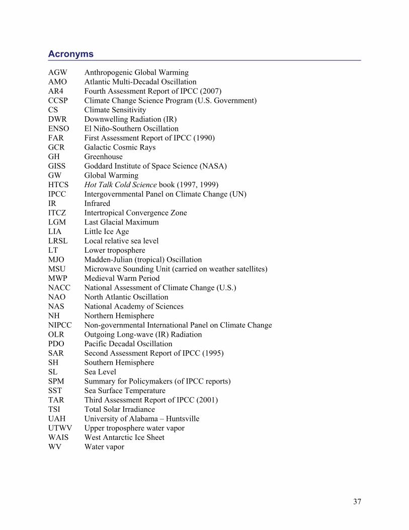
37

Acronyms

AGW Anthropogenic Global WarmingAMO Atlantic Multi-Decadal OscillationAR4 Fourth Assessment Report of IPCC (2007)CCSP Climate Change Science Program (U.S. Government)CS Climate SensitivityDWR Downwelling Radiation (IR)ENSO El Niño-Southern OscillationFAR First Assessment Report of IPCC (1990)GCR Galactic Cosmic RaysGH GreenhouseGISS Goddard Institute of Space Science (NASA)GW Global WarmingHTCS Hot Talk Cold Science book (1997, 1999)IPCC Intergovernmental Panel on Climate Change (UN)IR InfraredITCZ Intertropical Convergence ZoneLGM Last Glacial MaximumLIA Little Ice AgeLRSL Local relative sea levelLT Lower troposphereMJO Madden-Julian (tropical) OscillationMSU Microwave Sounding Unit (carried on weather satellites)MWP Medieval Warm PeriodNACC National Assessment of Climate Change (U.S.)NAO North Atlantic OscillationNAS National Academy of SciencesNH Northern HemisphereNIPCC Non-governmental International Panel on Climate ChangeOLR Outgoing Long-wave (IR) RadiationPDO Pacific Decadal OscillationSAR Second Assessment Report of IPCC (1995)SH Southern HemisphereSL Sea LevelSPM Summary for Policymakers (of IPCC reports)SST Sea Surface TemperatureTAR Third Assessment Report of IPCC (2001)TSI Total Solar IrradianceUAH University of Alabama – HuntsvilleUTWV Upper troposphere water vaporWAIS West Antarctic Ice SheetWV Water vapor

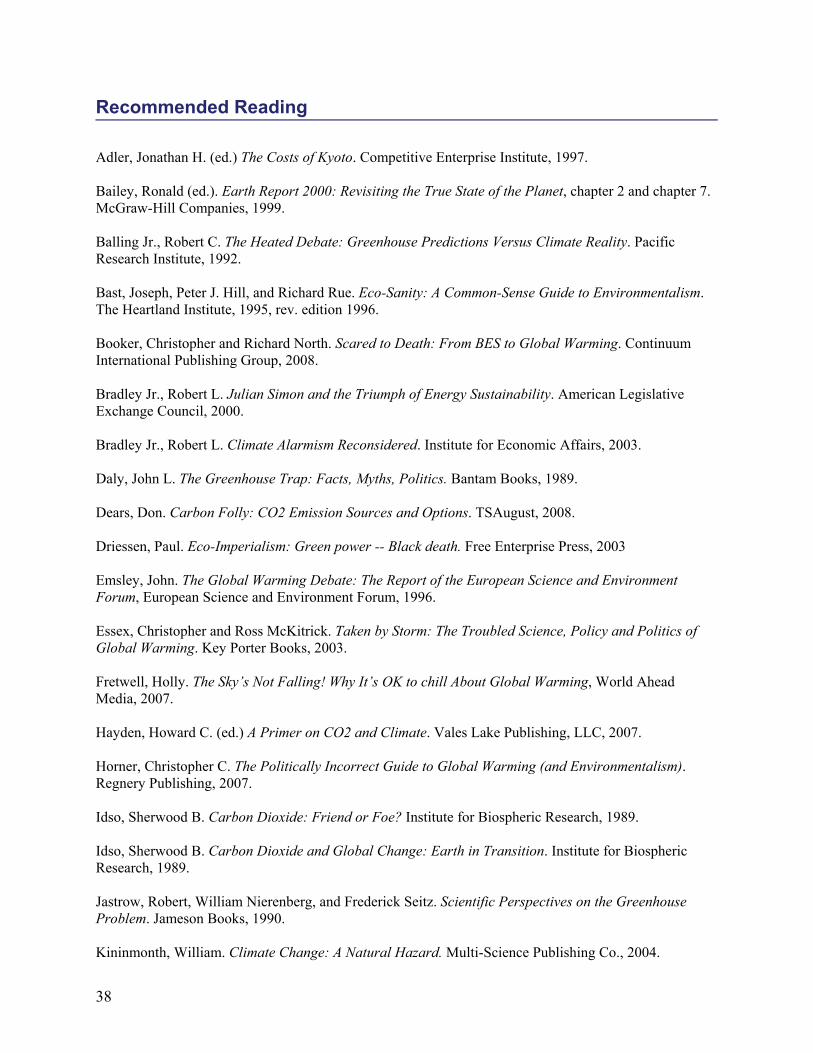
38

Recommended Reading

Adler, Jonathan H. (ed.) The Costs of Kyoto. Competitive Enterprise Institute, 1997.

Bailey, Ronald (ed.). Earth Report 2000: Revisiting the True State of the Planet, chapter 2 and chapter 7.McGraw-Hill Companies, 1999.

Balling Jr., Robert C. The Heated Debate: Greenhouse Predictions Versus Climate Reality. PacificResearch Institute, 1992.

Bast, Joseph, Peter J. Hill, and Richard Rue. Eco-Sanity: A Common-Sense Guide to Environmentalism.The Heartland Institute, 1995, rev. edition 1996.

Booker, Christopher and Richard North. Scared to Death: From BES to Global Warming. ContinuumInternational Publishing Group, 2008.

Bradley Jr., Robert L. Julian Simon and the Triumph of Energy Sustainability. American LegislativeExchange Council, 2000.

Bradley Jr., Robert L. Climate Alarmism Reconsidered. Institute for Economic Affairs, 2003.

Daly, John L. The Greenhouse Trap: Facts, Myths, Politics. Bantam Books, 1989.

Dears, Don. Carbon Folly: CO2 Emission Sources and Options. TSAugust, 2008.

Driessen, Paul. Eco-Imperialism: Green power -- Black death. Free Enterprise Press, 2003

Emsley, John. The Global Warming Debate: The Report of the European Science and EnvironmentForum, European Science and Environment Forum, 1996.

Essex, Christopher and Ross McKitrick. Taken by Storm: The Troubled Science, Policy and Politics ofGlobal Warming. Key Porter Books, 2003.

Fretwell, Holly. The Sky’s Not Falling! Why It’s OK to chill About Global Warming, World AheadMedia, 2007.

Hayden, Howard C. (ed.) A Primer on CO2 and Climate. Vales Lake Publishing, LLC, 2007.

Horner, Christopher C. The Politically Incorrect Guide to Global Warming (and Environmentalism).Regnery Publishing, 2007.

Idso, Sherwood B. Carbon Dioxide: Friend or Foe? Institute for Biospheric Research, 1989.

Idso, Sherwood B. Carbon Dioxide and Global Change: Earth in Transition. Institute for BiosphericResearch, 1989.

Jastrow, Robert, William Nierenberg, and Frederick Seitz. Scientific Perspectives on the GreenhouseProblem. Jameson Books, 1990.

Kininmonth, William. Climate Change: A Natural Hazard. Multi-Science Publishing Co., 2004.

39

Labohm, Hans, Simon Rozendaal, and Dick Thoenes. Man-Made Global Warming: Unraveling a Dogma.Multi-Science Publishing Co., 2004.

Lawson, Nigel. An Appeal to Reason: A Cool Look at Global Warming. Duckworth Overlook, 2008.

Lehr, Jay H. (ed.). Rational Readings on Environmental Concerns. Wiley, 1992.

Lehr, Jay H. and Janet Lehr (eds.). Standard Handbook of Environmental Science, Health, andTechnology, chapter 22, section 1. McGraw-Hill Professional, 2000.

Lomborg, Bjorn. Cool It: The skeptical Environmentalist’s Guide to Global Warming. Knopf, 2007.

Mathiesen, Mihkel. Global Warming in a Politically Correct Climate: How Truth Became Controversial.iUniverse, 2004.

Mendelsohn, Robert and James E. Neumann (eds.). The Impact of Climate Change on the United StatesEconomy. Cambridge University Press, 1999.

Michaels, Patrick J. Shattered Consensus: The True State of Global Warming. Rowman & Littlefield,2005.

Michaels, Patrick J. Meltdown: The Predictable Distortion of Global Warming by Scientists, Politicians,and the Media. Cato Institute, 2005.

Michaels, Patrick J. and Robert C. Balling, Jr.. The Satanic Gases: Clearing the Air about GlobalWarming. Cato Institute, 2000.

Milloy, Steven and Michael Gough. Silencing Science. Cato Institute, 1998.

Moore, Thomas Gale. Climate of Fear: Why We Shouldn’t Worry about Global Warming. Cato Institute,1998.

Nordhaus, William D. (ed.) Economics and Policy Issues in Climate Change. Resources for the Future,1998.

Okonski, Kendra (ed.). Adapt or Die: The Science, Politics and Economics of Climate Change. ProfileBusiness, 2003.

Ray, Dixy Lee with Lou Guzzo. Environmental Overkill: Whatever Happened to Common Sense?Perennial, 1994.

Singer, S. Fred (ed.). Global Effects of Environmental Pollution. Reidel, 1970.

Singer, S. Fred (ed.). The Changing Global Environment. Reidel, 1975.

Singer, S. Fred (ed.). Global Climate Change: Human and Natural Influences. Paragon House, 1989.

Singer, S. Fred. Hot Talk, Cold Science: Global Warming’s Unfinished Debate. Independent Institute,1997, rev. ed. 1999.

40

Singer, S. Fred and Dennis Avery. Unstoppable Global Warming: Every 1,500 Years. Rowman &Littlefield Publishers, Inc., 2007

Solomon, Lawrence. The Deniers: The World Renowned Scientists Who Stood Up Against GlobalWarming Hysteria, Political Persecution, and Fraud – And those Who Are Too Afraid to Do So. RichardVigilante Books, 2008.

Soon, Willie and S.H. Yaskell. The Maunder Minimum and the Variable Sun-Earth Connection. WorldScientific Publishing Co., 2003.

Spencer, Roy. Climate Confusion: How Global Warming Leads to Bad Science, Pandering politiciansand Misguided Policies that Hurt the Poor. Encounter Books, 2008.

Svensmark, Henrik and Nigel Calder. The Chilling Stars: A New Theory of Climate Change. Icon Books,2007.

Tuba, Zoltan (ed.). Ecolological Responses and Adaptations of Crops to Rising Atmospheric CarbonDioxide. Food Products Press, 2005.

Walker, Charls E. , Mark A. Bloomfield, and Margo Thorning (eds.). Climate Change Policy: PracticalStrategies to Promote Economic Growth and Environmental Quality. American Council for CapitalFormation, 1999.

Weber, Gerd R Global Warming: The Rest of the Story. Dr Boettiger Verlag, 1992.

Wildavsky, Aaron. But Is it True? A Citizen’s Guide to Environmental Health and Safety Issues. HarvardUniversity Press, 1997.

Wittwer, S.H. Food, Climate and Carbon Dioxide. CRC Press, 1995.