Natural Disasters and Plant Survival: the impact of the ...
51
Natural Disasters and Plant Survival: The Impact of the Kobe Earthquake Matthew A Cole University of Birmingham, UK Robert J R Elliott University of Birmingham, UK Toshihiro Okubo Keio University, Japan Eric Strobl Ecole Polytechnique, France
Transcript of Natural Disasters and Plant Survival: the impact of the ...
Natural Disasters and Plant Survival:
The Impact of the Kobe Earthquake
Matthew A Cole University of Birmingham, UK
Robert J R Elliott
University of Birmingham, UK
Toshihiro Okubo Keio University, Japan
Eric Strobl
Ecole Polytechnique, France
INTRODUCTION
Natural disasters can have a devastating impact on infrastructure,
households and firms in the affected area
Understanding what exactly this impact is can aid in disaster
preparedness and mitigation
There has been surprisingly little research and most of what has been
done has tended to focus on cross-country and regional studies that
estimate the overall impact of particular events on economic growth
(Loayza et al. 2009, Hochrainer 2009, Hallegatte and Dumas 2009 and
Ahlerup 2013)
Result: generally only short-term negative or positive impact
INTRODUCTION
Of the different types of natural disaster earthquakes represent one
of the most devastating
Earthquake damage can be primary and secondary consisting of
physical damage to buildings and infrastructure and disruption to
electricity/gas/water supplies
Earthquakes can also have a unique impact on plant activity as plants
in a relatively small geographical area can be impacted very
differently
THIS PAPER
We examine the impact of the Kobe EQ on plant performance
Relevant Literature:
Kobe earthquake: Horwich (2000) – no net impact at the macro-level
Firm level analysis:
o Craioneanu & Terrell (2010) – larger firms are more likely to
reopen after Hurricane Katrina;
o Leiter et al (2009) employment growth in European firms is higher
in regions with greater floods;
o Hosono et al (2012) firms’ investment decreases with banks in
more affected Kobe regions
But: These all use regional or imprecise measures of actual damage
THIS PAPER
Our contribution:
Using geo-coding techniques we generate a measure of the damage
incurred by individual buildings in the Kobe earthquake zone which
we combine with manufacturing plant level data
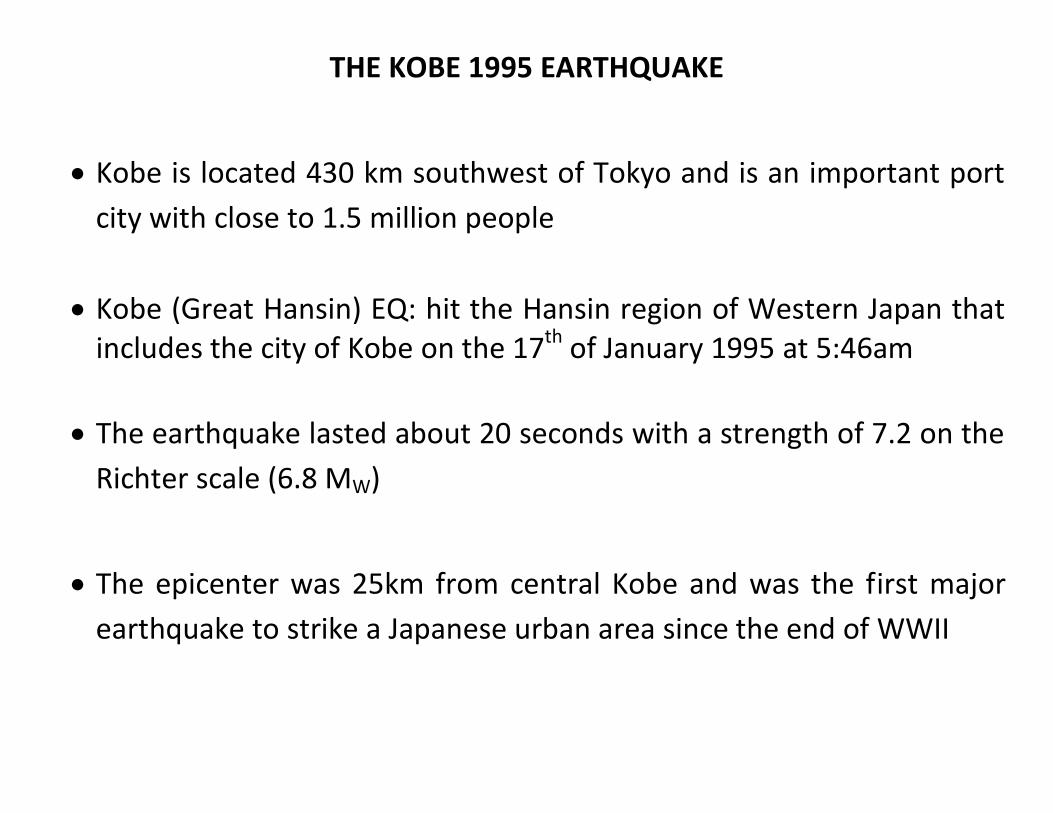
THE KOBE 1995 EARTHQUAKE
Kobe is located 430 km southwest of Tokyo and is an important port
city with close to 1.5 million people
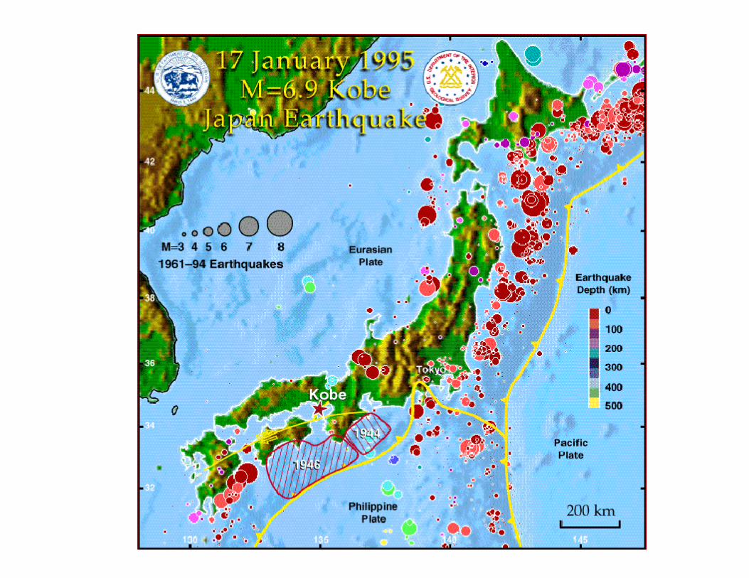
Kobe (Great Hansin) EQ: hit the Hansin region of Western Japan that includes the city of Kobe on the 17th of January 1995 at 5:46am
The earthquake lasted about 20 seconds with a strength of 7.2 on the
Richter scale (6.8 MW)
The epicenter was 25km from central Kobe and was the first major
earthquake to strike a Japanese urban area since the end of WWII
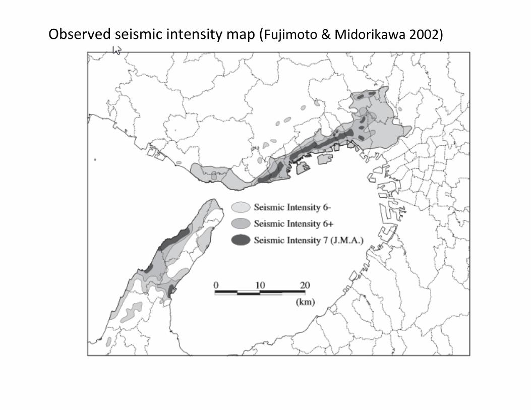
Observed seismic intensity map (Fujimoto & Midorikawa 2002)
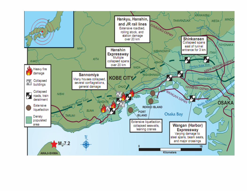
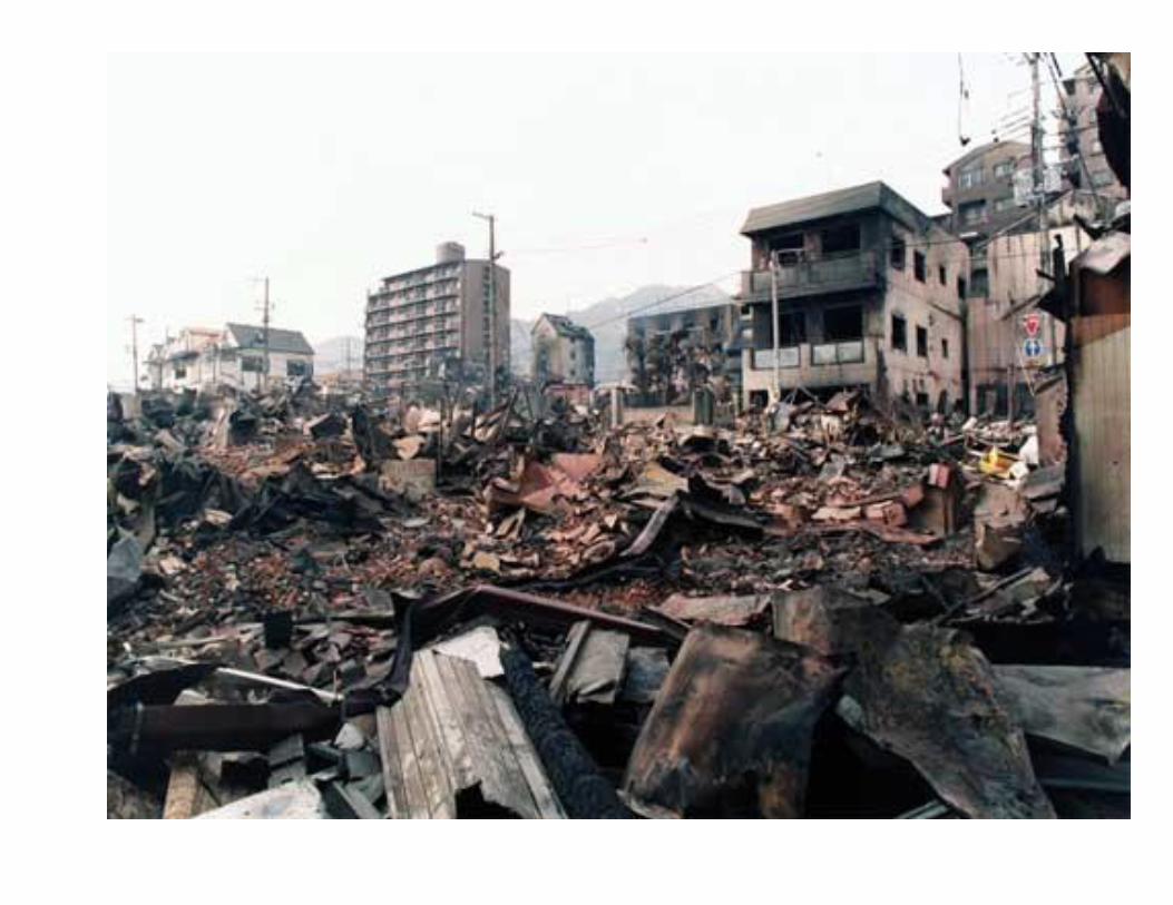
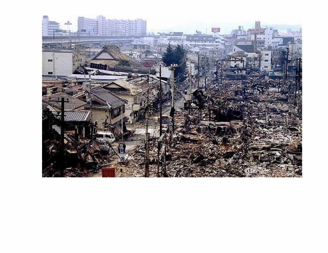
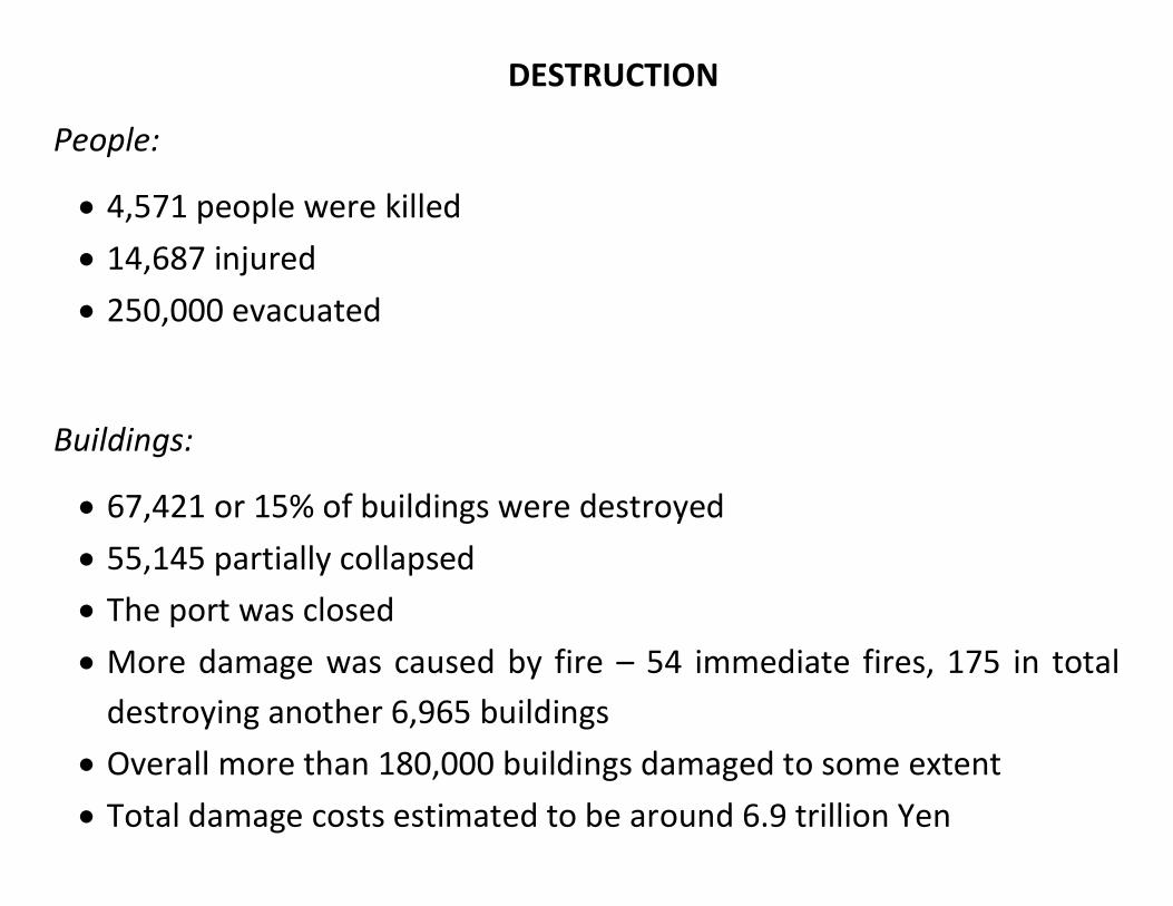
DESTRUCTION
People:
4,571 people were killed
14,687 injured
250,000 evacuated
Buildings:
67,421 or 15% of buildings were destroyed
55,145 partially collapsed
The port was closed
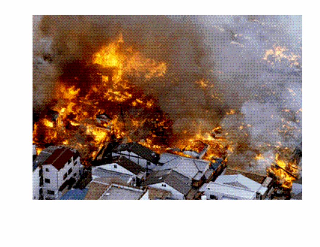
More damage was caused by fire – 54 immediate fires, 175 in total
destroying another 6,965 buildings
Overall more than 180,000 buildings damaged to some extent
Total damage costs estimated to be around 6.9 trillion Yen
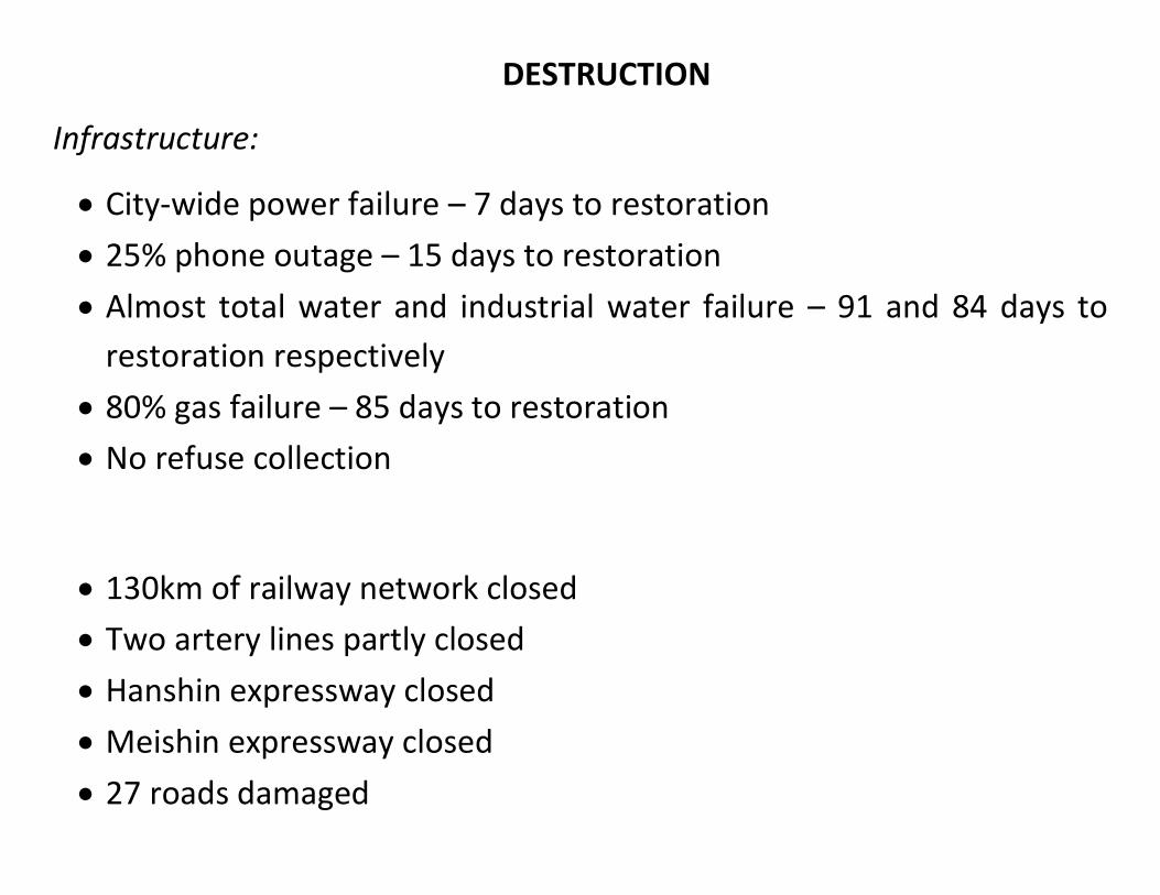
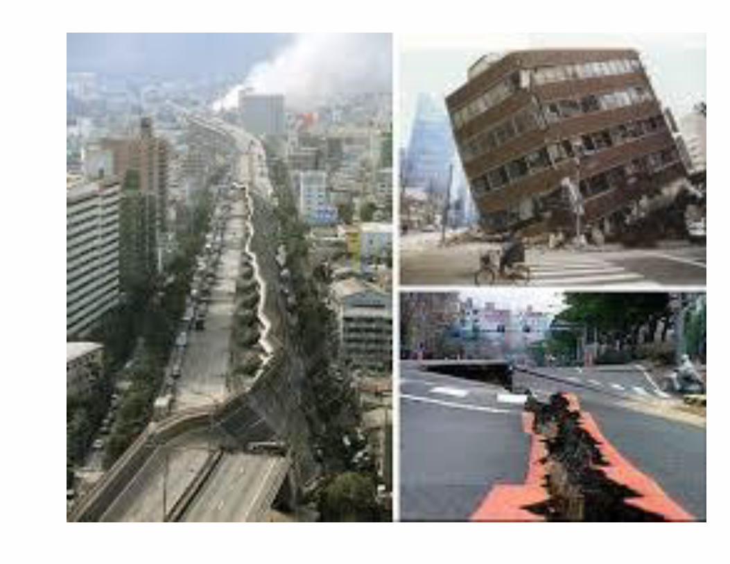
DESTRUCTION
Infrastructure:
City-wide power failure – 7 days to restoration
25% phone outage – 15 days to restoration
Almost total water and industrial water failure – 91 and 84 days to
restoration respectively
80% gas failure – 85 days to restoration
No refuse collection
130km of railway network closed
Two artery lines partly closed
Hanshin expressway closed
Meishin expressway closed
27 roads damaged
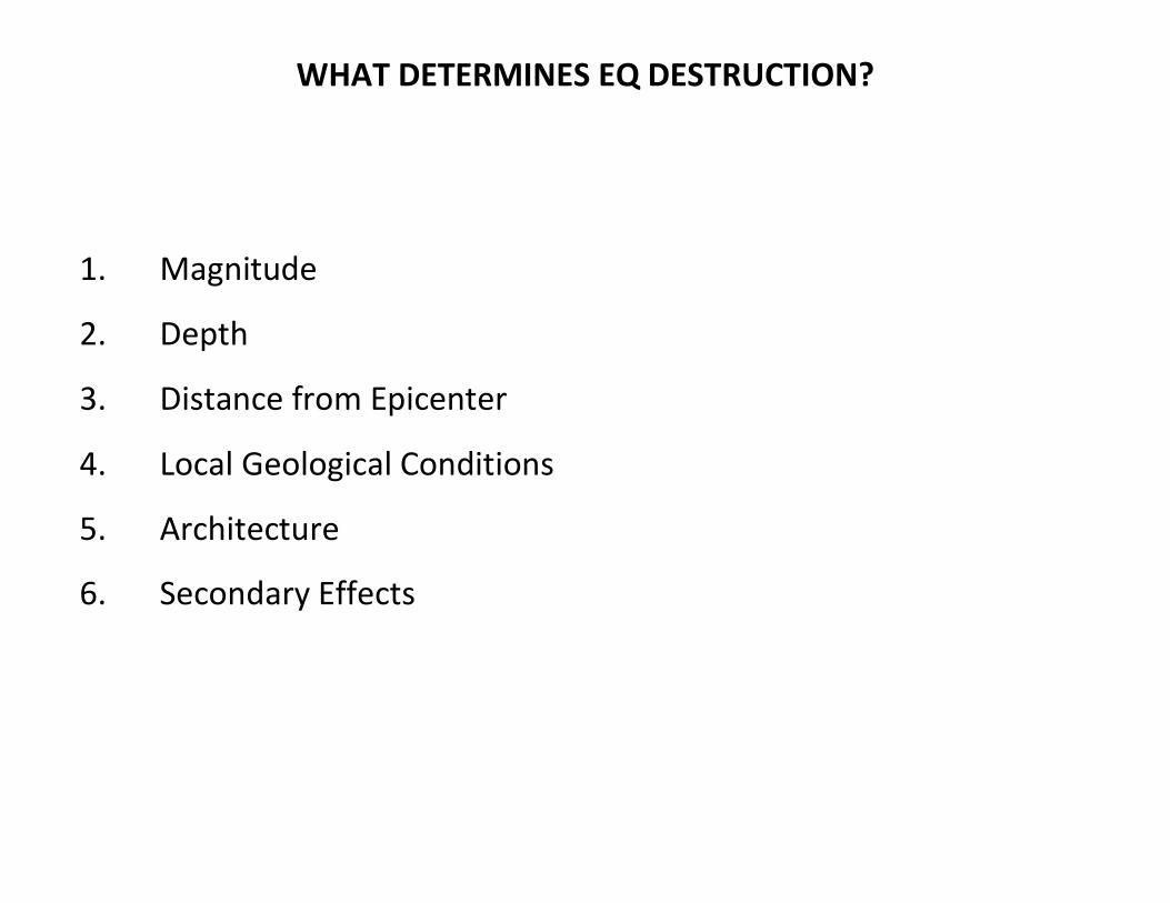
WHAT DETERMINES EQ DESTRUCTION?
1. Magnitude
2. Depth
3. Distance from Epicenter
4. Local Geological Conditions
5. Architecture
6. Secondary Effects
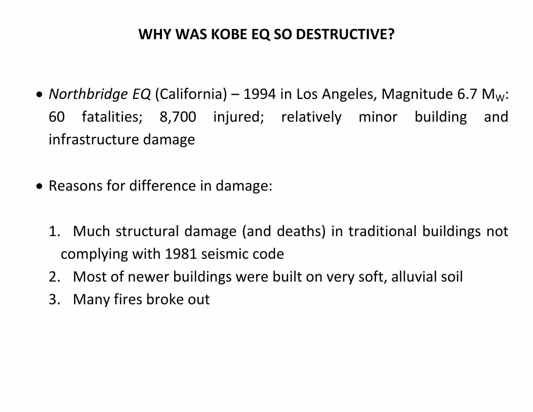
WHY WAS KOBE EQ SO DESTRUCTIVE?
Northbridge EQ (California) – 1994 in Los Angeles, Magnitude 6.7 MW:
60 fatalities; 8,700 injured; relatively minor building and
infrastructure damage
Reasons for difference in damage:
1. Much structural damage (and deaths) in traditional buildings not
complying with 1981 seismic code
2. Most of newer buildings were built on very soft, alluvial soil
3. Many fires broke out
DATA
Manufacturing Plant Data:
We utilise the Japanese Manufacturing Census and the Establishment
and Enterprise Census - 1,846 manufacturing plants in Kobe city from
1992 to 2007
Plants are followed until their death or until the end of our sample
period in 2008
The Manufacturing Census and the Establishment and Enterprise
Census are exhaustive with no minimum size for inclusion
Contains information on: exact address, sector, production,
employment, wages, age, etc.

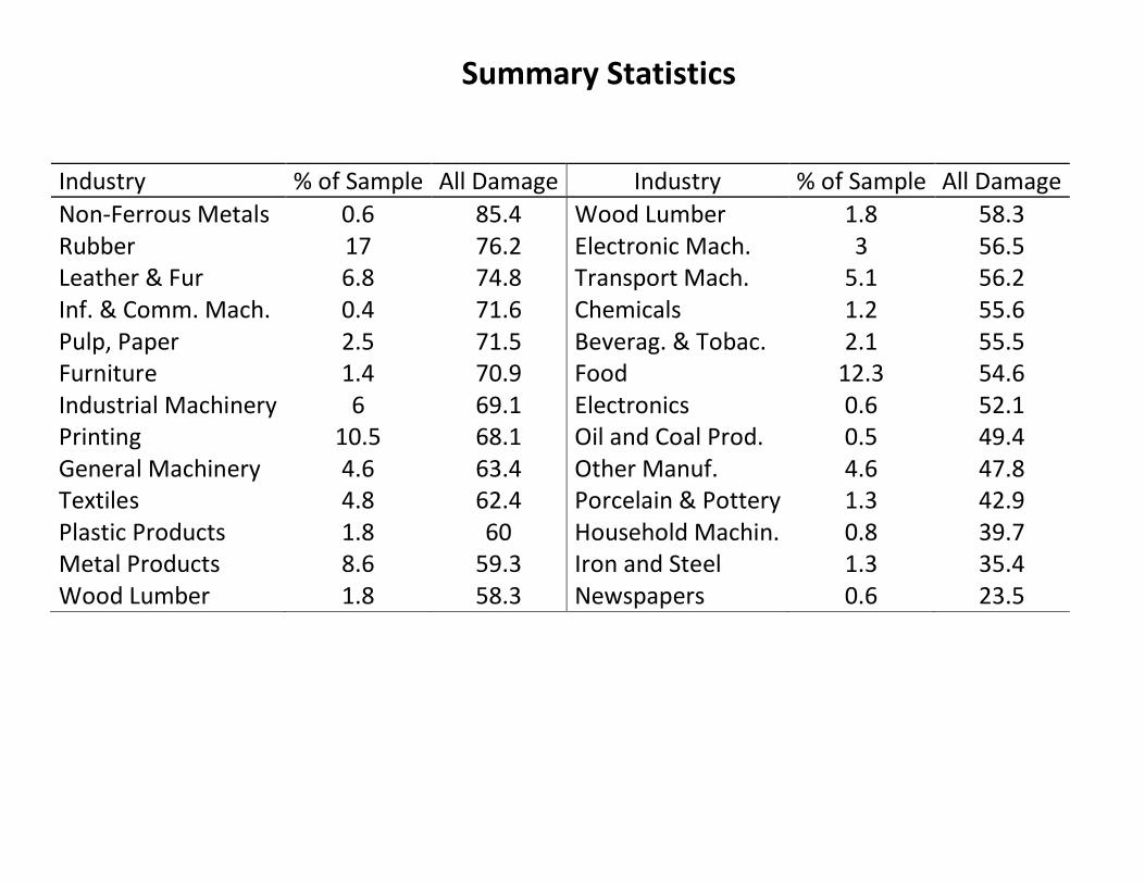
Summary Statistics
Industry % of Sample All Damage Industry % of Sample All Damage
Non-Ferrous Metals 0.6 85.4 Wood Lumber 1.8 58.3 Rubber 17 76.2 Electronic Mach. 3 56.5 Leather & Fur 6.8 74.8 Transport Mach. 5.1 56.2 Inf. & Comm. Mach. 0.4 71.6 Chemicals 1.2 55.6 Pulp, Paper 2.5 71.5 Beverag. & Tobac. 2.1 55.5 Furniture 1.4 70.9 Food 12.3 54.6 Industrial Machinery 6 69.1 Electronics 0.6 52.1 Printing 10.5 68.1 Oil and Coal Prod. 0.5 49.4 General Machinery 4.6 63.4 Other Manuf. 4.6 47.8 Textiles 4.8 62.4 Porcelain & Pottery 1.3 42.9 Plastic Products 1.8 60 Household Machin. 0.8 39.7 Metal Products 8.6 59.3 Iron and Steel 1.3 35.4 Wood Lumber 1.8 58.3 Newspapers 0.6 23.5
DATA
Damage Data:
Source: (1) ‘Shinsai Hukkou Akaibu’ (archive on the damage of the
1995 Hyogo-Awaji earthquake) by Kobe City Office; (2) Toru
Fukushima (University of Hyogo), (3) ‘Zenrin’s Residential Map,
Hyogo-ken Kobe city 1995’ from Toru Fukushima (University of
Hyogo)
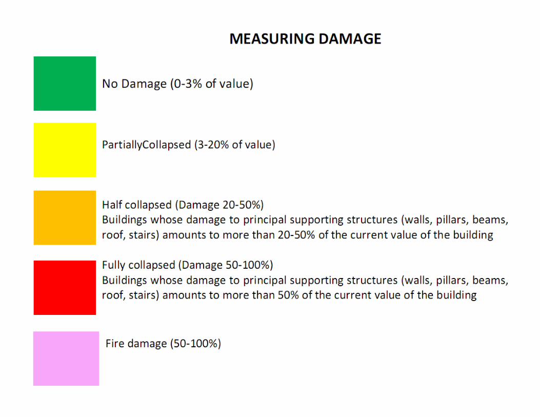
These sources provide a highly detailed building map of Kobe and
assign one of 5 colours to each building to categorize damage
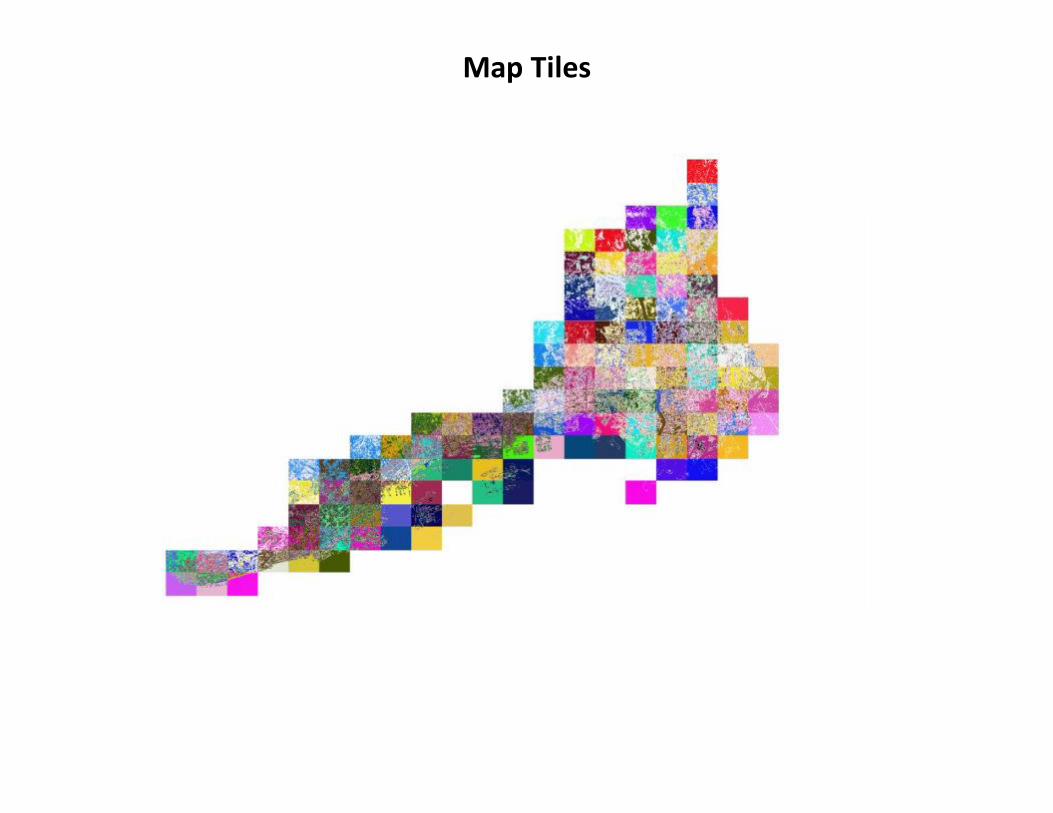
Map Tiles
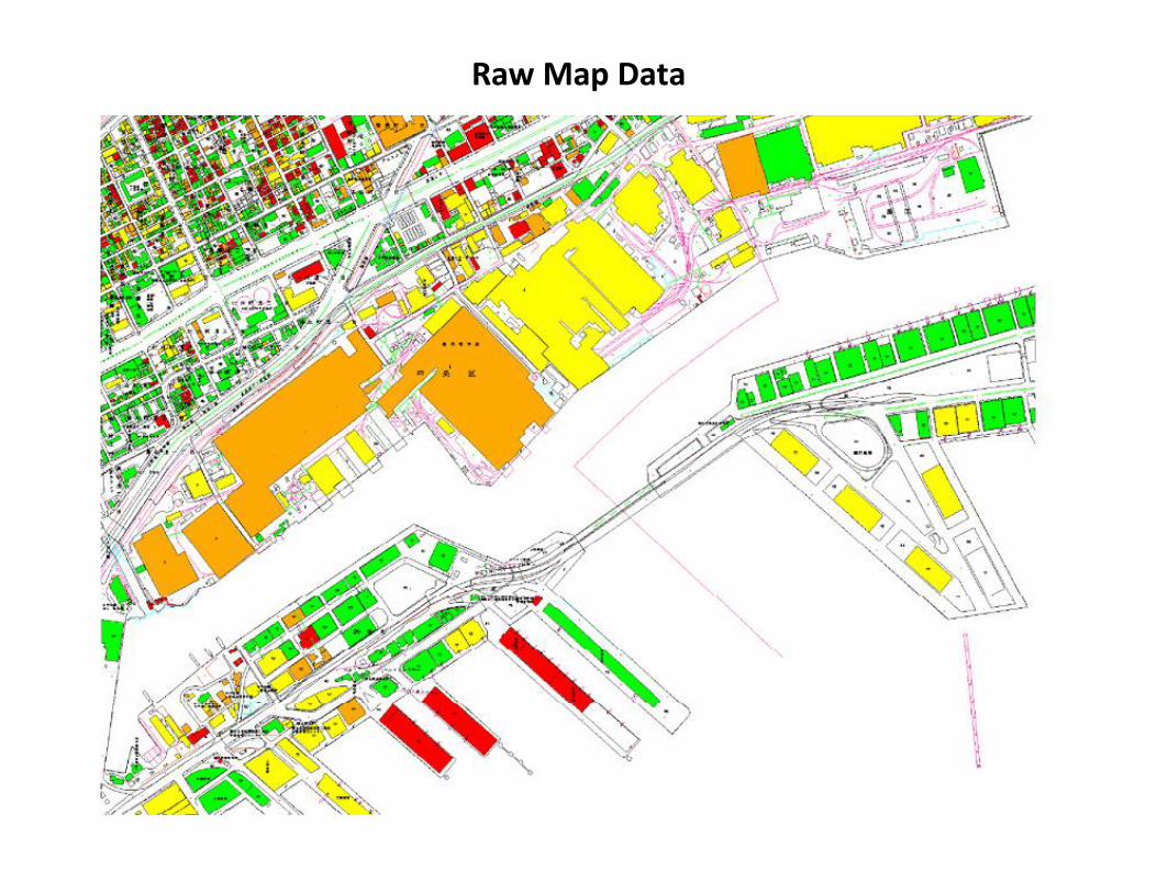
Raw Map Data
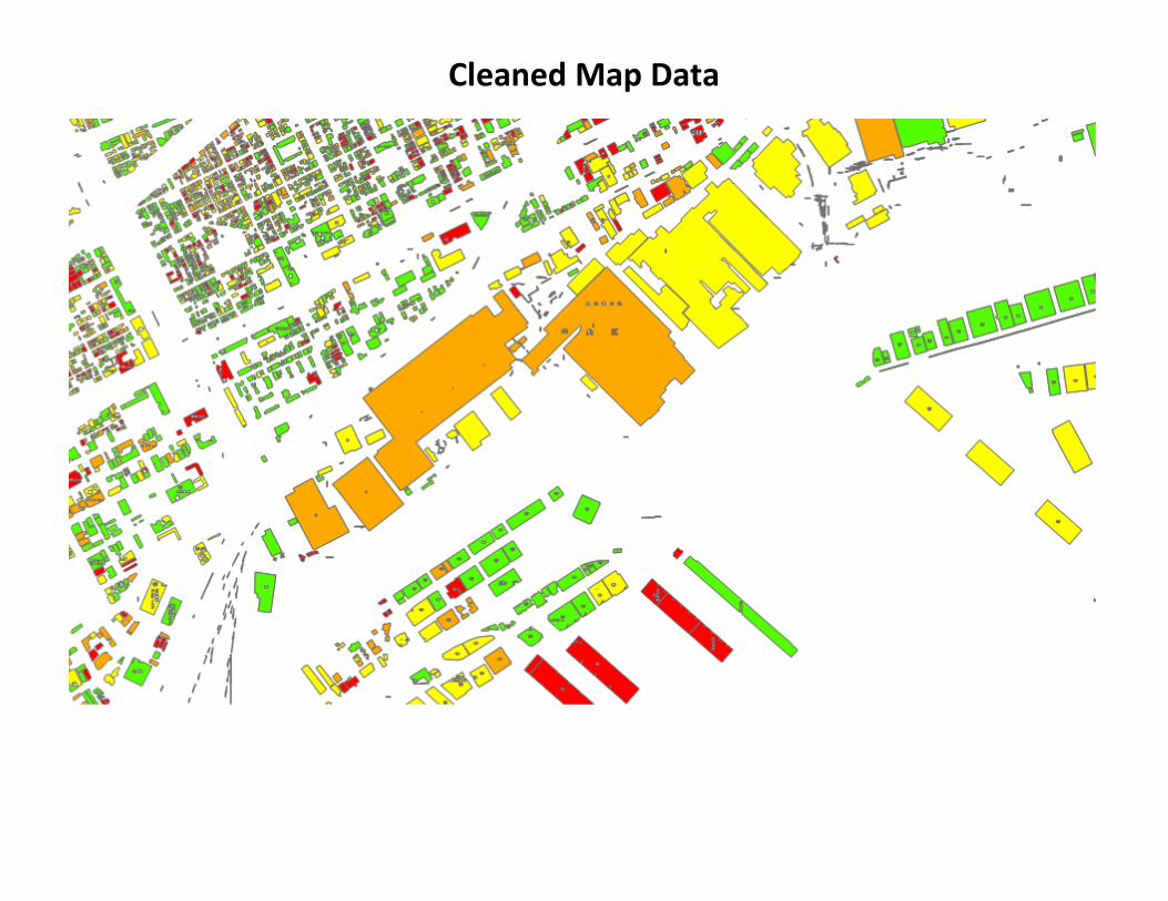
Cleaned Map Data
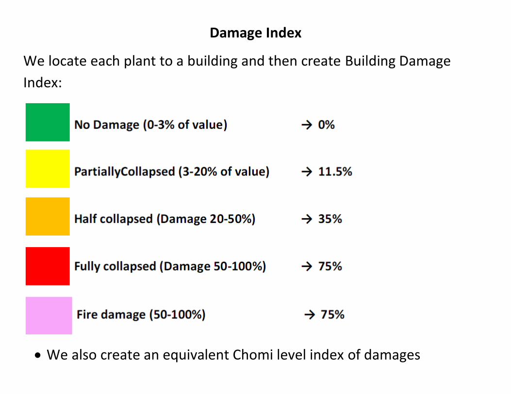
Damage Index
We locate each plant to a building and then create Building Damage
Index:
We also create an equivalent Chomi level index of damages
Summary Statistics
Industry % of Sample All Damage Industry % of Sample All Damage
Non-Ferrous Metals 0.6 85.4 Wood Lumber 1.8 58.3 Rubber 17 76.2 Electronic Mach. 3 56.5 Leather & Fur 6.8 74.8 Transport Mach. 5.1 56.2 Inf. & Comm. Mach. 0.4 71.6 Chemicals 1.2 55.6 Pulp, Paper 2.5 71.5 Beverag. & Tobac. 2.1 55.5 Furniture 1.4 70.9 Food 12.3 54.6 Industrial Machinery 6 69.1 Electronics 0.6 52.1 Printing 10.5 68.1 Oil and Coal Prod. 0.5 49.4 General Machinery 4.6 63.4 Other Manuf. 4.6 47.8 Textiles 4.8 62.4 Porcelain & Pottery 1.3 42.9 Plastic Products 1.8 60 Household Machin. 0.8 39.7 Metal Products 8.6 59.3 Iron and Steel 1.3 35.4 Wood Lumber 1.8 58.3 Newspapers 0.6 23.5
Estimation
Goal: Estimate impact on survival and post survival performance
Y= f(damage index, X)
Is the damage index truly exogenous?
(1) The Kobe earthquake as an exogenous shock
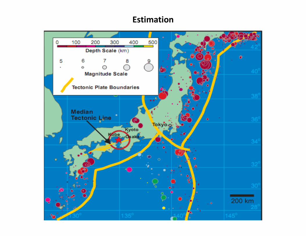
(2) EQs are spatial phenomena
Estimation
(1) The Kobe earthquake was arguably an unanticipated shock
“The news that Kobe was directly hit by an earthquake had major
repercussions throughout Japan, particularly because of the enormity of
the damage and, at the same time, due to the fact that Kobe could be
struck by an earthquake. During the 1,500 years that earthquake
occurrence has been recorded in Japan, not once has Kobe been directly
hit by an earthquake and it has always had the image of being a city safe
from earthquakes” Kaji Hideki, UNRCD Director
“Few businesses or private households held earthquake insurance.
Indeed, most losses were uninsured: only 3% of property in the Kobe area
was covered by earthquake indemnity, compared to 16% in Tokyo.”
(Edington, 2010)
Estimation
Estimation
(2) EQs are spatial phenomena
So we also control for:
a. Chomi level characteristics: share of buildings by type (cement,
wood, brick, iron); share of buildings by age category;
b. Plant level characteristics: Age, size, wage, TFP, sector, whether
moved, whether multi-plant etc.
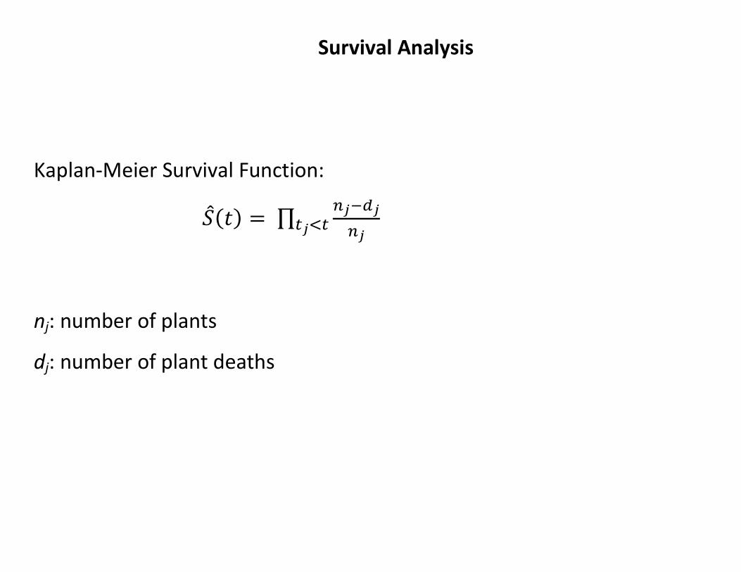
Survival Analysis
Kaplan-Meier Survival Function:
nj: number of plants
dj: number of plant deaths
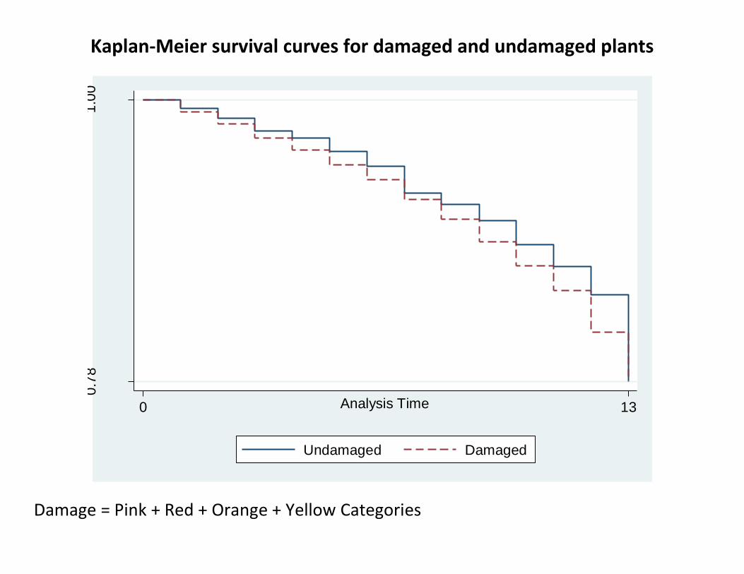
Kaplan-Meier survival curves for damaged and undamaged plants
Damage = Pink + Red + Orange + Yellow Categories
0.7
81
.00
0 13Analysis Time
Undamaged Damaged
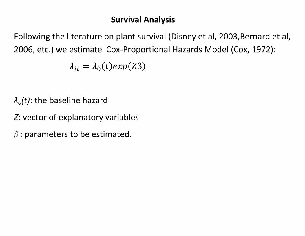
Survival Analysis
Following the literature on plant survival (Disney et al, 2003,Bernard et al,
2006, etc.) we estimate Cox-Proportional Hazards Model (Cox, 1972):
λ0(t): the baseline hazard
Z: vector of explanatory variables
β : parameters to be estimated.
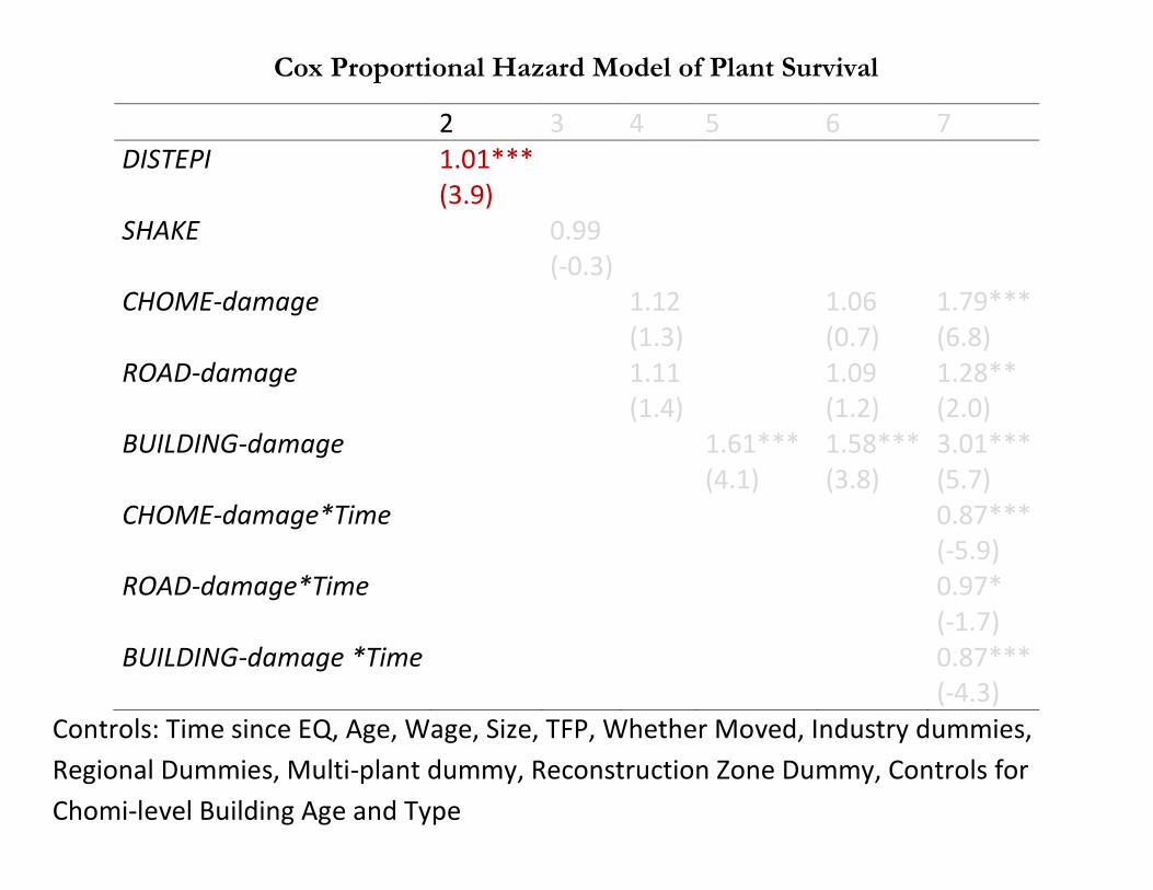
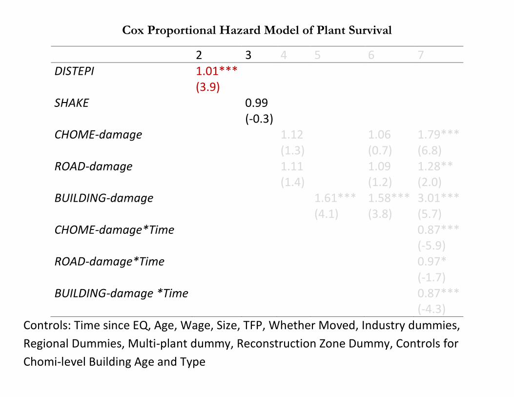
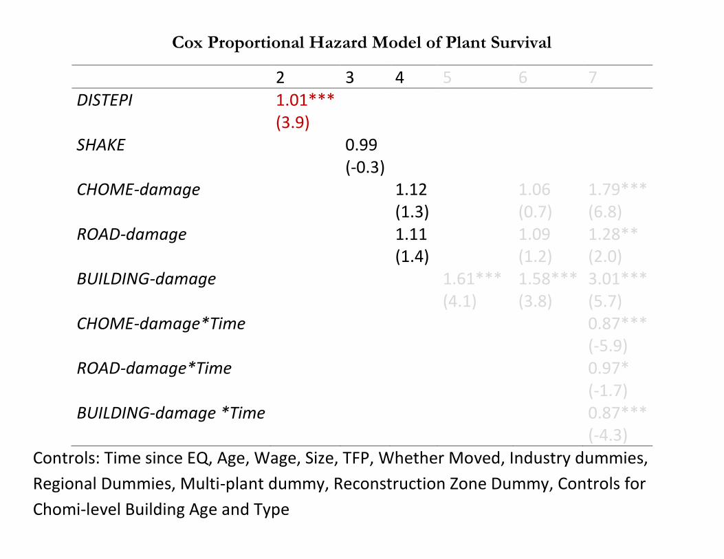
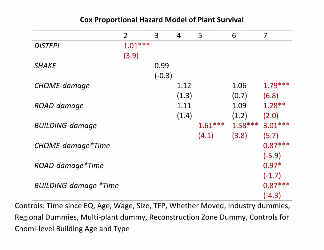
Cox Proportional Hazard Model of Plant Survival
2 3 4 5 6 7 DISTEPI 1.01***
(3.9)
SHAKE
0.99 (-0.3)
CHOME-damage 1.12 1.06 1.79*** (1.3) (0.7) (6.8) ROAD-damage 1.11 1.09 1.28** (1.4) (1.2) (2.0) BUILDING-damage 1.61*** 1.58*** 3.01*** (4.1) (3.8) (5.7) CHOME-damage*Time 0.87***
(-5.9) ROAD-damage*Time 0.97*
(-1.7) BUILDING-damage *Time 0.87***
(-4.3)
Controls: Time since EQ, Age, Wage, Size, TFP, Whether Moved, Industry dummies,
Regional Dummies, Multi-plant dummy, Reconstruction Zone Dummy, Controls for
Chomi-level Building Age and Type
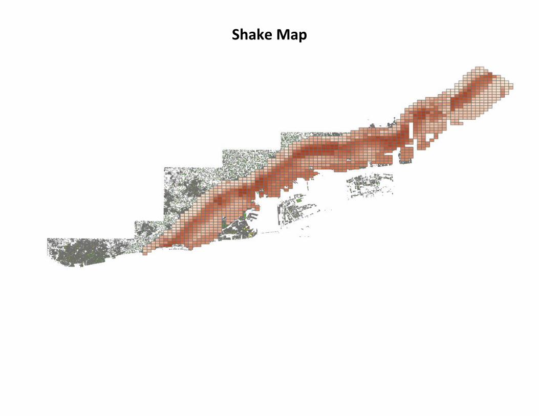
Shake Map
Cox Proportional Hazard Model of Plant Survival
2 3 4 5 6 7 DISTEPI 1.01***
(3.9)
SHAKE
0.99 (-0.3)
CHOME-damage 1.12 1.06 1.79*** (1.3) (0.7) (6.8) ROAD-damage 1.11 1.09 1.28** (1.4) (1.2) (2.0) BUILDING-damage 1.61*** 1.58*** 3.01*** (4.1) (3.8) (5.7) CHOME-damage*Time 0.87***
(-5.9) ROAD-damage*Time 0.97*
(-1.7) BUILDING-damage *Time 0.87***
(-4.3)
Controls: Time since EQ, Age, Wage, Size, TFP, Whether Moved, Industry dummies,
Regional Dummies, Multi-plant dummy, Reconstruction Zone Dummy, Controls for
Chomi-level Building Age and Type
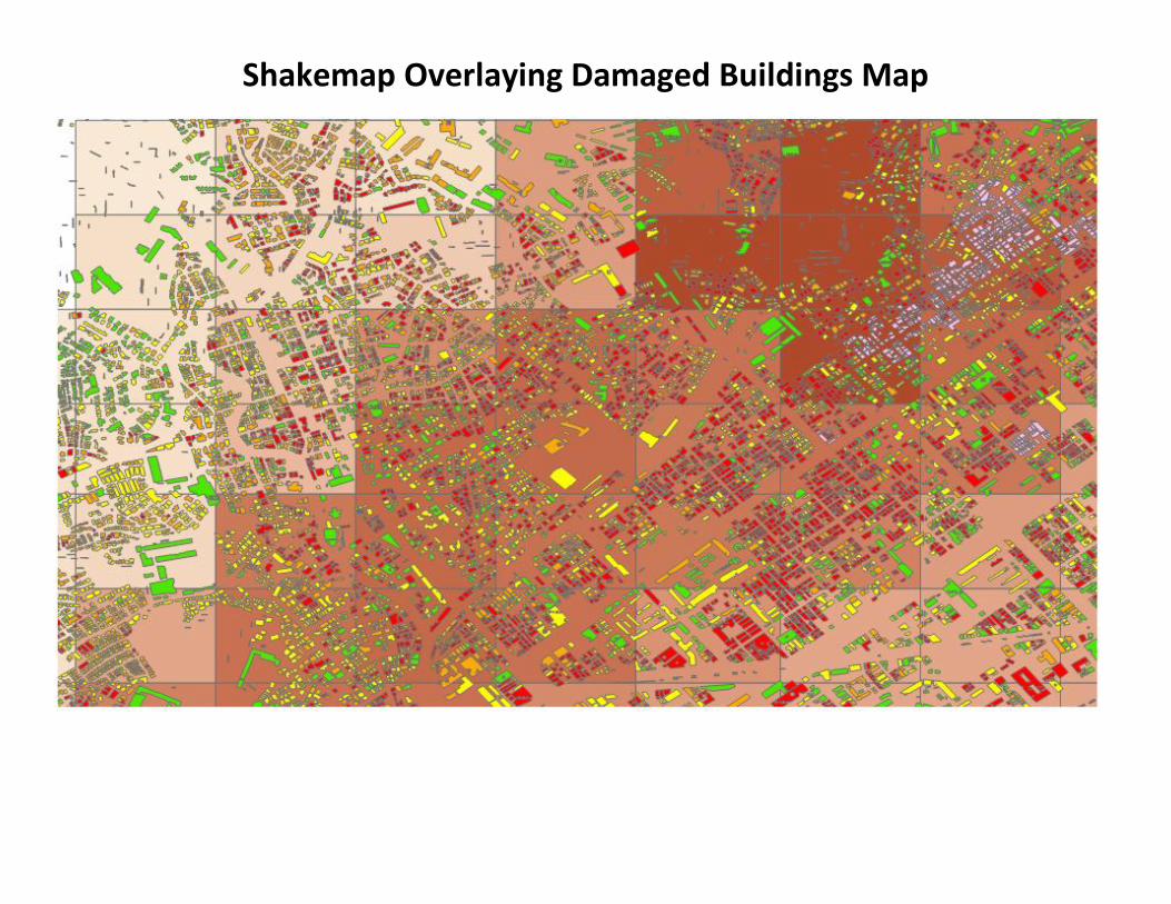
Shakemap Overlaying Damaged Buildings Map
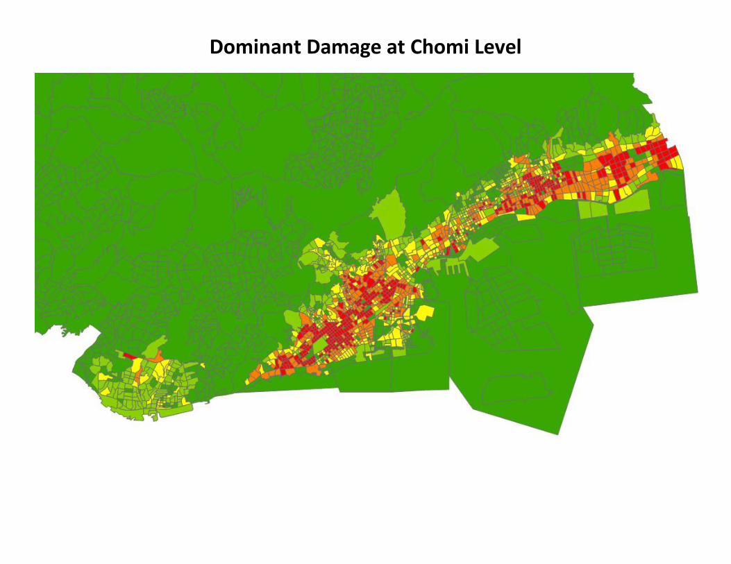
Dominant Damage at Chomi Level
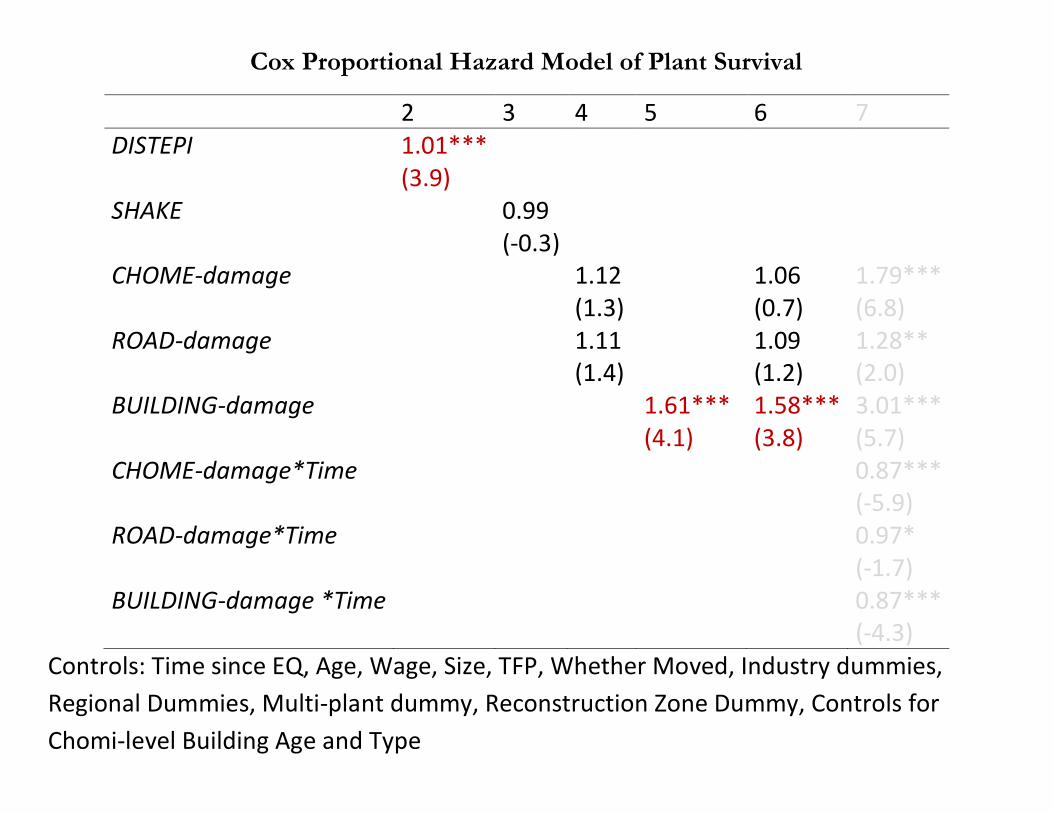
Cox Proportional Hazard Model of Plant Survival
2 3 4 5 6 7 DISTEPI 1.01***
(3.9)
SHAKE
0.99 (-0.3)
CHOME-damage 1.12 1.06 1.79*** (1.3) (0.7) (6.8) ROAD-damage 1.11 1.09 1.28** (1.4) (1.2) (2.0) BUILDING-damage 1.61*** 1.58*** 3.01*** (4.1) (3.8) (5.7) CHOME-damage*Time 0.87***
(-5.9) ROAD-damage*Time 0.97*
(-1.7) BUILDING-damage *Time 0.87***
(-4.3)
Controls: Time since EQ, Age, Wage, Size, TFP, Whether Moved, Industry dummies,
Regional Dummies, Multi-plant dummy, Reconstruction Zone Dummy, Controls for
Chomi-level Building Age and Type
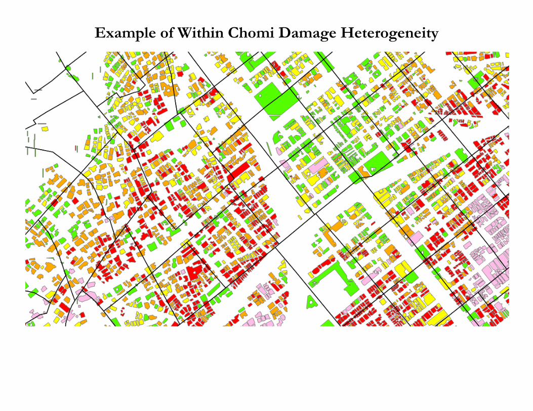
Example of Within Chomi Damage Heterogeneity
Cox Proportional Hazard Model of Plant Survival
2 3 4 5 6 7 DISTEPI 1.01***
(3.9)
SHAKE
0.99 (-0.3)
CHOME-damage 1.12 1.06 1.79*** (1.3) (0.7) (6.8) ROAD-damage 1.11 1.09 1.28** (1.4) (1.2) (2.0) BUILDING-damage 1.61*** 1.58*** 3.01*** (4.1) (3.8) (5.7) CHOME-damage*Time 0.87***
(-5.9) ROAD-damage*Time 0.97*
(-1.7) BUILDING-damage *Time 0.87***
(-4.3)
Controls: Time since EQ, Age, Wage, Size, TFP, Whether Moved, Industry dummies,
Regional Dummies, Multi-plant dummy, Reconstruction Zone Dummy, Controls for
Chomi-level Building Age and Type
Damage Impact over time
Impact is unlikely to be permanent, but may vary over time because of:
1. Plants may struggle before they shut down
2. Government Aid may help some of them to survive for some time
Cox Proportional Hazard Model of Plant Survival
2 3 4 5 6 7
DISTEPI 1.01*** (3.9)
SHAKE
0.99 (-0.3)
CHOME-damage 1.12 1.06 1.79*** (1.3) (0.7) (6.8) ROAD-damage 1.11 1.09 1.28** (1.4) (1.2) (2.0) BUILDING-damage 1.61*** 1.58*** 3.01*** (4.1) (3.8) (5.7) CHOME-damage*Time 0.87***
(-5.9) ROAD-damage*Time 0.97*
(-1.7) BUILDING-damage *Time 0.87***
(-4.3)
Controls: Time since EQ, Age, Wage, Size, TFP, Whether Moved, Industry dummies,
Regional Dummies, Multi-plant dummy, Reconstruction Zone Dummy, Controls for
Chomi-level Building Age and Type
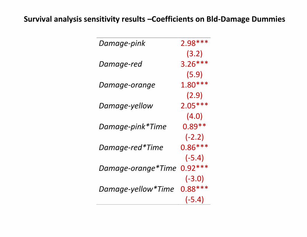
Survival analysis sensitivity results –Coefficients on Bld-Damage Dummies
Damage-pink 2.98*** (3.2) Damage-red 3.26*** (5.9) Damage-orange 1.80*** (2.9) Damage-yellow 2.05*** (4.0) Damage-pink*Time 0.89** (-2.2) Damage-red*Time 0.86*** (-5.4) Damage-orange*Time 0.92*** (-3.0) Damage-yellow*Time 0.88*** (-5.4)
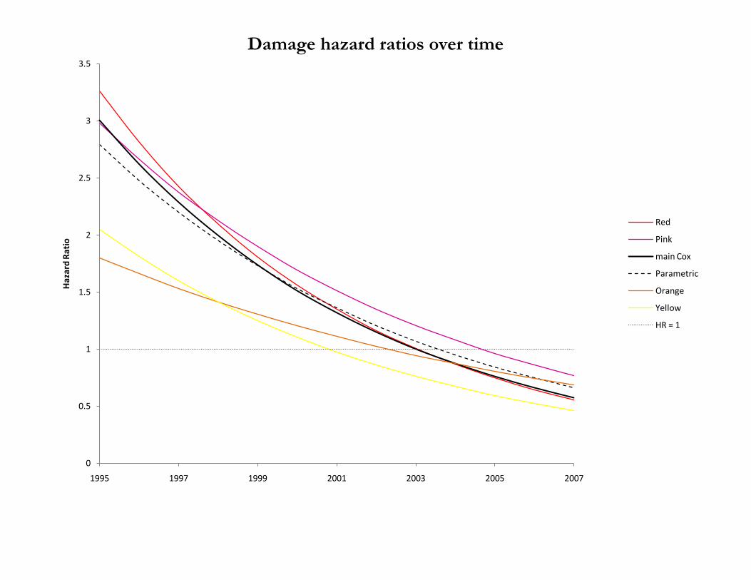
Damage hazard ratios over time
0
0.5
1
1.5
2
2.5
3
3.5
1995 1997 1999 2001 2003 2005 2007
Haz
ard
Rat
io
Red
Pink
main Cox
Parametric
Orange
Yellow
HR = 1
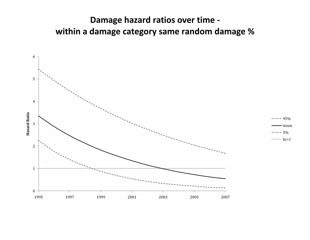
Damage hazard ratios over time - within a damage category same random damage %
0
1
2
3
4
5
6
1995 1997 1999 2001 2003 2005 2007
Ha
zard
Ra
tio
95%
mean
5%
hr=1
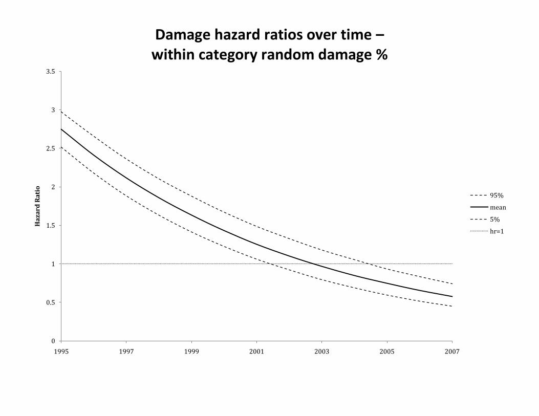
Damage hazard ratios over time – within category random damage %
0
0.5
1
1.5
2
2.5
3
3.5
1995 1997 1999 2001 2003 2005 2007
Ha
zard
Ra
tio
95%
mean
5%
hr=1

Creative Destruction?
Literature:
We examine two channels:
1. Impact on Survivors – fixed effects estimator; Unit of analysis: plants -level ;
period 1992-2008
2. New Entrants – Negative Binomial Model; Unit of analysis: Chomi level;
period: 1992-2008
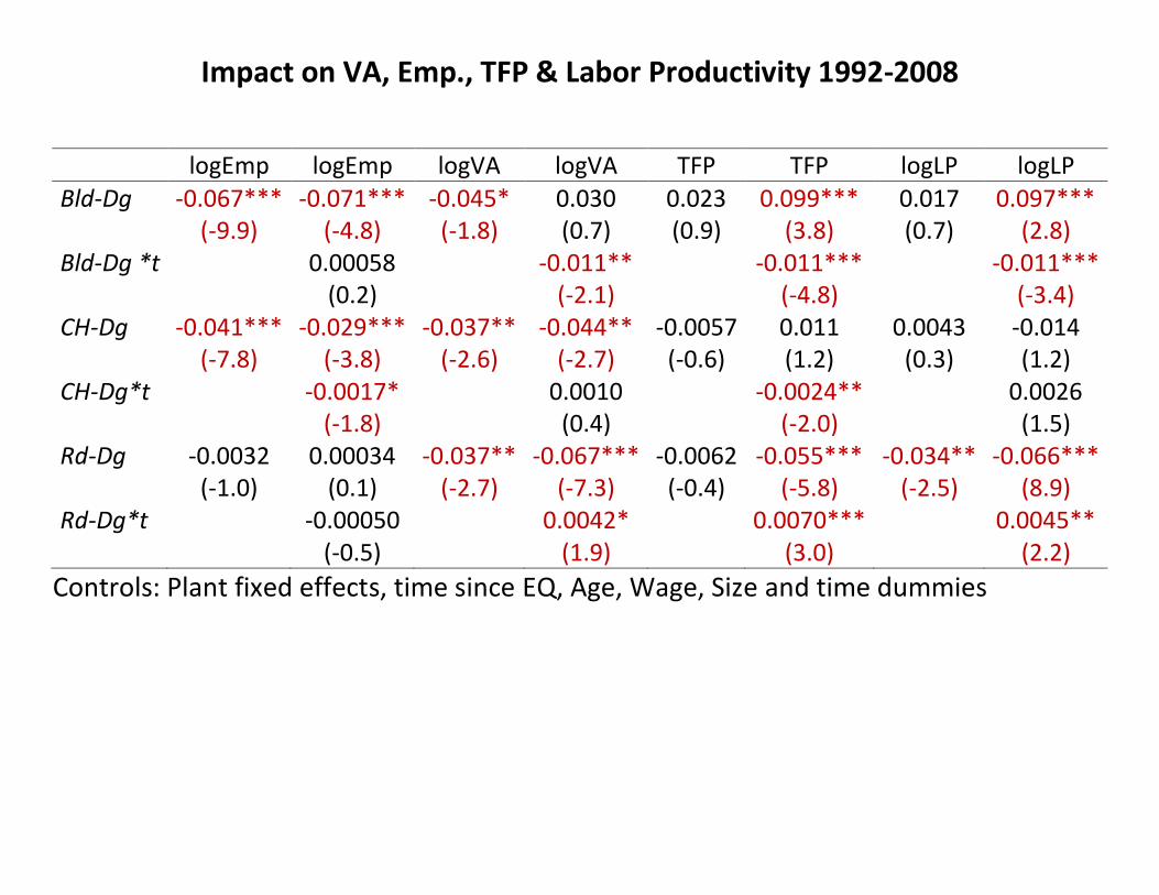
Impact on VA, Emp., TFP & Labor Productivity 1992-2008
logEmp logEmp logVA logVA TFP TFP logLP logLP
Bld-Dg -0.067*** (-9.9)
-0.071*** (-4.8)
-0.045* (-1.8)
0.030 (0.7)
0.023 (0.9)
0.099*** (3.8)
0.017 (0.7)
0.097*** (2.8)
Bld-Dg *t
0.00058 (0.2)
-0.011** (-2.1)
-0.011*** (-4.8)
-0.011*** (-3.4)
CH-Dg -0.041*** (-7.8)
-0.029*** (-3.8)
-0.037** (-2.6)
-0.044** (-2.7)
-0.0057 (-0.6)
0.011 (1.2)
0.0043 (0.3)
-0.014 (1.2)
CH-Dg*t
-0.0017* (-1.8)
0.0010 (0.4)
-0.0024** (-2.0)
0.0026 (1.5)
Rd-Dg -0.0032 0.00034 -0.037** -0.067*** -0.0062 -0.055*** -0.034** -0.066*** (-1.0) (0.1) (-2.7) (-7.3) (-0.4) (-5.8) (-2.5) (8.9) Rd-Dg*t -0.00050 0.0042* 0.0070*** 0.0045** (-0.5) (1.9) (3.0) (2.2)
Controls: Plant fixed effects, time since EQ, Age, Wage, Size and time dummies
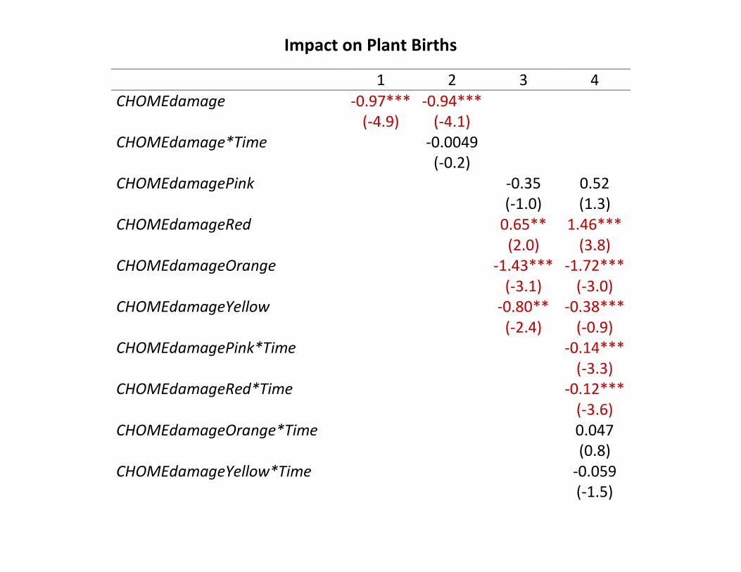
Impact on Plant Births
1 2 3 4
CHOMEdamage -0.97*** -0.94*** (-4.9) (-4.1) CHOMEdamage*Time -0.0049 (-0.2) CHOMEdamagePink -0.35 0.52 (-1.0) (1.3) CHOMEdamageRed 0.65** 1.46*** (2.0) (3.8) CHOMEdamageOrange -1.43*** -1.72*** (-3.1) (-3.0) CHOMEdamageYellow -0.80** -0.38*** (-2.4) (-0.9) CHOMEdamagePink*Time -0.14*** (-3.3) CHOMEdamageRed*Time -0.12*** (-3.6) CHOMEdamageOrange*Time 0.047 (0.8) CHOMEdamageYellow*Time -0.059 (-1.5)
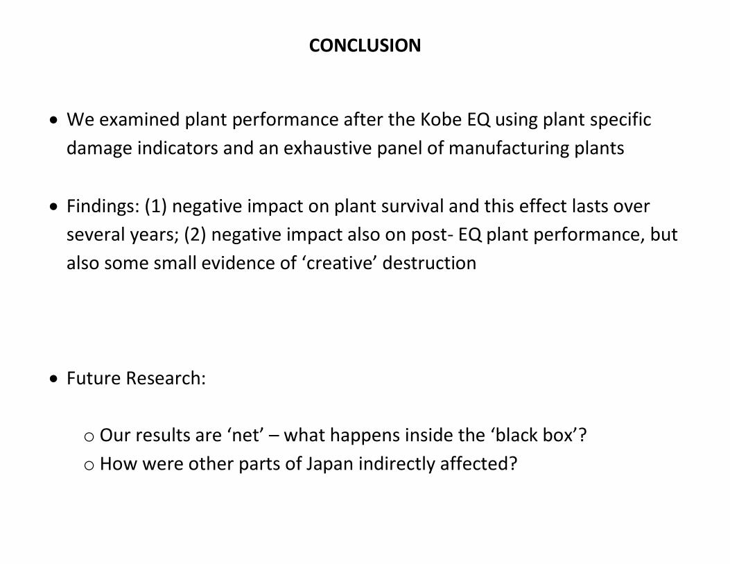
CONCLUSION
We examined plant performance after the Kobe EQ using plant specific
damage indicators and an exhaustive panel of manufacturing plants
Findings: (1) negative impact on plant survival and this effect lasts over
several years; (2) negative impact also on post- EQ plant performance, but
also some small evidence of ‘creative’ destruction
Future Research:
o Our results are ‘net’ – what happens inside the ‘black box’?
o How were other parts of Japan indirectly affected?