Policy Research Working Paper 8188

Natural Disaster Damage Indices Based on Remotely Sensed Data

An Application to Indonesia

Emmanuel Skoufias Eric Strobl

Thomas Tveit

Poverty and Equity Global Practice GroupSeptember 2017

WPS8188P

ublic

Dis

clos

ure

Aut

horiz

edP

ublic

Dis

clos

ure

Aut

horiz

edP

ublic

Dis

clos

ure

Aut

horiz

edP

ublic

Dis

clos

ure

Aut

horiz

ed

Produced by the Research Support Team

Abstract

The Policy Research Working Paper Series disseminates the findings of work in progress to encourage the exchange of ideas about development issues. An objective of the series is to get the findings out quickly, even if the presentations are less than fully polished. The papers carry the names of the authors and should be cited accordingly. The findings, interpretations, and conclusions expressed in this paper are entirely those of the authors. They do not necessarily represent the views of the International Bank for Reconstruction and Development/World Bank and its affiliated organizations, or those of the Executive Directors of the World Bank or the governments they represent.

Policy Research Working Paper 8188

This paper is a product of the Poverty and Equity Global Practice Group. It is part of a larger effort by the World Bank to provide open access to its research and make a contribution to development policy discussions around the world. Policy Research Working Papers are also posted on the Web at http://econ.worldbank.org. The authors may be contacted at eskoufias@worldbank.org.

Combining nightlight data as a proxy for economic activity with remote sensing data typically used for natural hazard modeling, this paper constructs novel damage indices at the district level for Indonesia, for different disaster events such as floods, earthquakes, volcanic eruptions and the 2004 Christmas Tsunami. Ex ante, prior to the incidence of a disas-ter, district-level damage indices could be used to determine

the size of the annual fiscal transfers from the central gov-ernment to the subnational governments. Ex post, or after the incidence of a natural disaster, damage indices are useful for quickly assessing and estimating the damages caused and are especially useful for central and local governments, emergency services, and aid workers so that they can respond efficiently and deploy resources where they are most needed.

Natural Disaster Damage Indices Based on Remotely Sensed

Data: An Application to Indonesia∗

Emmanuel Skoufias (World Bank)Eric Strobl (University of Bern)

Thomas Tveit (University of Cergy-Pontoise)

JEL Classification: Q54, C63, R11, R5,O18Keywords: Remotely Sensed Data, Natural Disasters, Natural Hazard model, Damage Index, Floods,Earthquakes, Volcanic Eruptions

∗This paper was financed in part by the Disaster Risk Finance Impact Analytics project of the Disaster Risk Financingand Insurance Program of The World Bank Group

1 Introduction

Quickly assessing and estimating the damage caused after the incidence of a natural disaster is importantfor both central and local governments, emergency services and aid workers, so that they can respondefficiently and deploy resources where they are most needed. Recently, remote sensing technologies havebeen used to analyze the impact of disasters, such as hurricanes (Myint et al., 2008; Klemas, 2009),floods (Haq et al., 2012; Wu et al., 2012, 2014; Chung et al., 2015), landslides (Nichol et al., 2006),earthquakes (Fu et al., 2005; Yamazaki & Matsuoka, 2007), wildfires (Holden et al., 2005; Roy et al.,2006), volcanoes (Carn et al., 2009; Ferguson et al., 2010) and tsunamis (Romer et al., 2012). Theseremote sensing techniques are useful for providing quick damage estimates shortly after the disastersgiving emergency services a chance to respond quickly and local governments an overview of estimatedcosts and necessary repairs.

In addition to their usefulness in the aftermath of a disaster, estimates of the potential damage as-sociated with a natural disaster are also useful for policy making prior to the realization of the naturalhazard event. In many cases the incidence of a natural hazard event can turn into a natural disastersimply because of inadequate preparation ex-ante. Indonesia, for example, is highly exposed to naturaldisasters by being situated in one of the worlds most active disaster hot spots, where several types ofdisasters such as earthquakes, tsunamis, volcanic eruptions, floods, landslides, droughts and forest firesfrequently occur. The average annual cost of natural disasters, over the last 10 years, is estimated at 0.3percent of Indonesian GDP, although the economic impact of such disasters is generally much higher atlocal or subnational levels (The Global Facility for Disaster Reduction and Recovery, 2011). The highfrequency of disasters experienced has important impacts on expenditures by local governments thatcould be anticipated, at least in part, through upward adjustments in the annual fiscal transfers fromthe central government to the subnational governments.1 Such ex-ante adjustments in the level of fiscaltransfers would be more useful if they could be based on estimates of the potential damages associatedwith the incidence of a natural disaster as opposed to estimates of the intensity of the potential naturalhazard that might occur. However, although in recent years there has been much progress towards themodeling of the main natural hazards, there continues to be a scarcity of estimates of the damagesassociated with the incidence of these disasters. The value of damage caused by a natural disaster is typ-ically a complicated function of the size of population living in that area, the level and type of economicactivity carried out, the value of the physical infrastructure in place, and the resilience of infrastructureand people’s livelihoods to the natural hazards.

This paper fills some of the gaps in the literature by using different remote sensing sources and dataon the physical characteristics of the events to construct four damage indices for natural disasters inIndonesia. The indices cover floods, earthquakes, volcanic eruptions and a tsunami, and are all weightedby local economic activity in an area, and then aggregated up to a district level.2 All data used in theconstruction of the indices are free and publicly available, making the methods used a potentially veryuseful alternative for both central and local governments to quickly get a rough estimate of the damagescaused by a disaster (either ex-ante or ex-post).3

Importantly, all of the indices constructed take into account local exposure. Given limited accessto highly disaggregated local economic activity data, nightlight intensity derived from satellite imageryhas proved to be a good proxy; see, for instance, Henderson et al. (2012), Hodler & Raschky (2014) andMichalopoulos & Papaioannou (2014). By utilizing the grid cells of approximately 1 square kilometer wecan break down areas in cities and districts into where they are busiest, and thus take into account notonly the local physical characteristics of a natural disaster but also the local economic activity exposedto it.

The paper is structured as follows. Section 2 of the paper discusses in more detail the incidence andtypes of natural disasters. Section 3 discusses the nightlights data. Sections 4-7 discuss in detail theconstruction of the four damage indices, while section 8 concludes.

1For example, Indonesia experienced 4,000 disasters between 2001 and 2007 alone, including floods (37%), droughts(24%), landslides (11%) and windstorms (9%) (The Global Facility for Disaster Reduction and Recovery, 2011).

2A tropical cyclone index was also constructed, but no hurricanes had strong enough winds to cause any damage onland.

3In a separate paper, Skoufias et al. (2017), we correlate the damage indices of these disasters at the district level withthe ex-post allocation of district expenditures in different sectors and by economic classification.

2

2 Natural Disasters in Indonesia

Natural disasters are prevalent events across most parts of Indonesia. According to the Indonesian Na-tional Disaster Management Authority (BNPB) there were more than 19,000 natural disasters in theperiod 2001 - 2015 (National Disaster Management Agency, BNPB, 2016), making Indonesia a usefulcountry for any natural disaster analysis. The most frequent disasters are floods and landslides (52 per-cent), strong winds (21 percent) and fires (15 percent), while the most damaging ones are earthquakes,tsunamis and volcanic eruptions, which all cause major damage to buildings and infrastructure in ad-dition to the human casualties. The deadliest year according to the BNPB data was 2004, where therewere more than 167,000 deaths due to natural disasters and 166,671 of them stemming from the tsunamiin December 2004.

2.1 Floods

The tropical climate of Indonesia often leads to annual floods. The BNPB data registered more than10,000 incidents of floods or landslides leading to more than 3,500 fatalities from 2001 through 2015.During the period from 1985 to 2016, The Darthmouth Flood Observatory (DFO) registered 3,808 floodsof magnitude 4 or more and 1,175 floods of magnitude 6 and up.4 Of these floods, there were 126 largescale floods with a centroid within Indonesia in the period from 2001 to 2016 as can be seen in Figure 1.Of the 34 provinces, 27 experienced having a centroid of a large scale flood event during these years.5

Figure 1: DFO Large Scale Floods in Indonesia 2001-2016

Source: G.R.Brakenridge (2016)

4Magnitude is defined as: M = log(D ∗ S ∗ AA), where D is the duration of the flood; S is the severity on a scaleconsisting of 1 (large event), 1.5 (very large event) and 2 (extreme event); and AA is the size of the affected area. Floodevents registered by DFO have mainly been derived from news and governmental sources.

5The provinces where no large scale centroid was present were Bangka Belitung, Riau Islands, Kalimantan Barat,Yogyakarta, Sulawesi Barat, Kalimantan Utara and Maluku. Note that some of these, like Kalimantan Utara, KalimantanBarat, Sulawesi Barat and Yogakarta, did most likely experience large scale flood during these years, but that the centroidwas in another province. The remaining three provinces consist mainly of smaller islands, so the flooded area will mostlikely not constitute a large scale flood event.

3

2.2 Earthquakes

Due to Indonesia’s location inside the Pacific Ring of Fire, one of the most seismically active areas inthe world, it is often struck by earthquakes. BNPB counted almost 400 earthquakes from 2001 to 2015,with the largest number of casualties coming from the tsunami created by a 9.0 earthquake located offthe coast of Aceh, otherwise known as the earthquake that caused the 2004 tsunami. Apart from that,there were more than 8,000 registered fatalities due to earthquakes over the same period. Overall, thismakes earthquakes the deadliest of the natural disasters that strike Indonesia.

Figure 2 shows how common earthquakes are in Indonesia by displaying contour maps6 of all earth-quakes of magnitude 5.0 and above that struck Indonesia from 2004 through 2014. In total, the UnitedStates Geological Survey (USGS) registered 261 earthquakes.7

Figure 2: Earthquakes in Indonesia 2004-2014

Source: USGS

2.3 Volcanic activity

Indonesia has the highest number of active volcanoes in the world, numbering almost 150. Of these, manyhave had eruptions in both more historical times and after the year 2000. The most famous eruption isprobably the explosion of Krakatau in August 1883, when two-thirds of the Krakatau Island erupted anddisappeared, killing more than 35,000 people and causing a global mini ice age and weather disruptionsfor years. BNPB have registered 92 eruptions over our 15-year time period and more than 60 majorvolcanoes that have had eruptions since 1900. The most recent one is the 2010 Mount Merapi eruption

6These maps are also known as ShakeMaps, which are produced by USGS.7There are 1,002 earthquakes registered by USGS that were of magnitude 5.0 or more that had a point with a PGA of

at least 0.05 within Indonesia. Many of these points create little to no damage. The 261 earthquakes mentioned above arequakes that are mostly contained within Indonesia.

4

that killed 324 people and dislocated more than 320,000.

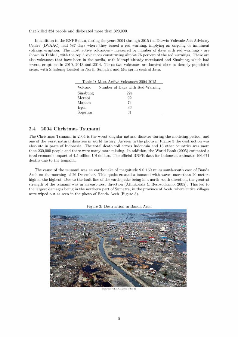
In addition to the BNPB data, during the years 2004 through 2015 the Darwin Volcanic Ash AdvisoryCentre (DVAAC) had 587 days where they issued a red warning, implying an ongoing or imminentvolcanic eruption. The most active volcanoes - measured by number of days with red warnings - areshown in Table 1, with the top 5 volcanoes constituting almost 75 percent of the red warnings. These arealso volcanoes that have been in the media, with Merapi already mentioned and Sinabung, which hadseveral eruptions in 2010, 2013 and 2014. These two volcanoes are located close to densely populatedareas, with Sinabung located in North Sumatra and Merapi in central Java.

Table 1: Most Active Volcanoes 2004-2015

Volcano Number of Days with Red Warning

Sinabung 224Merapi 92Manam 74Egon 36Soputan 31

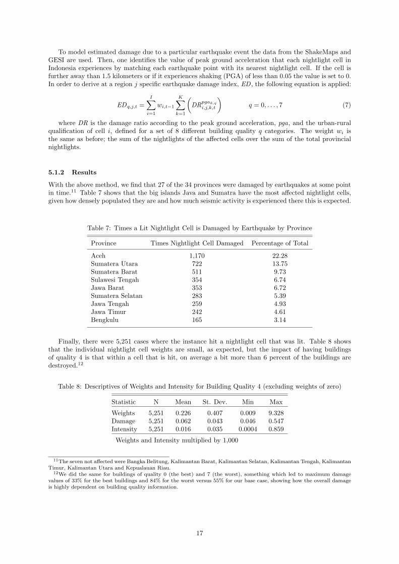
2.4 2004 Christmas Tsunami

The Christmas Tsunami in 2004 is the worst singular natural disaster during the modeling period, andone of the worst natural disasters in world history. As seen in the photo in Figure 3 the destruction wasabsolute in parts of Indonesia. The total death toll across Indonesia and 13 other countries was morethan 230,000 people and there were many more missing. In addition, the World Bank (2005) estimated atotal economic impact of 4.5 billion US dollars. The official BNPB data for Indonesia estimates 166,671deaths due to the tsunami.

The cause of the tsunami was an earthquake of magnitude 9.0 150 miles south-south east of BandaAceh on the morning of 26 December. This quake created a tsunami with waves more than 20 metershigh at the highest. Due to the fault line of the earthquake being in a north-south direction, the greateststrength of the tsunami was in an east-west direction (Athukorala & Resosudarmo, 2005). This led tothe largest damages being in the northern part of Sumatra, in the province of Aceh, where entire villageswere wiped out as seen in the photo of Banda Aceh (Figure 3).

Figure 3: Destruction in Banda Aceh

Source: The Atlantic (2014)

5

3 Nightlight Data

Natural disasters are inherent local phenomena in that they either affect only parts of areas and/oraffect parts within areas differently. It is thus important to take the local population/asset exposureinto account when constructing more aggregate proxies. Arguably one would like to have measures ofexposure as spatially disaggregated as possible. For a country like Indonesia, data are usually sparse andat a very aggregated spatial level.

An alternative approach is thus to use nightlights as a proxy for local economic activity. As a matterof fact, nightlights have found widespread use where no other measures are available; see, for instance,Henderson et al. (2012), Hodler & Raschky (2014) and Michalopoulos & Papaioannou (2014). In Hender-son et al. (2012), Indonesia is used as an example of using nightlights to capture an economic downturnfollowing the Asian financial crisis in the late 1990s. Their results show that swings in GDP change cangenerally be captured. Nevertheless one has to account for factors such as cultural differences in lightusage, latitude and gas flares. In our case this is unlikely to affect our results since we use nightlights tocapture exposure within a country rather than across countries.

The nightlight imagery we employ is provided by the Defense Meteorological Satellite Program(DMSP) satellites. In terms of coverage each DMSP satellite has a 101 minute near-polar orbit atan altitude of about 800km above the surface of the earth, providing global coverage twice per day, atthe same local time each day, with a spatial resolution of about 1km near the equator. The resultingimages provide the percentage of nightlight occurrences for each pixel per year normalized across satel-lites to a scale ranging from 0 (no light) to 63 (maximum light). Yearly values were then constructed assimple averages across daily values of grids, and are available from 1992.8 We use the stable, cloud-freeseries; see Elvidge et al. (1997).

The data revealed 414,644 cells which had a nightlight value greater than 0 in them at least onceduring the period 2001-2013. Figure 4 - containing all cells with nightlights in 2012 - shows that thelarge cities and densely populated areas on Java, Sunda Islands, coastal Kalimantan and Sumatra arefully covered in lights. Inner parts of Kalimantan and most parts of New Guinea are more sparsely lit.

Figure 4: Cells with Registered Nightlights in 2012

8For the years where satellites were replaced, DMSP provides an average from both the new and old satellite. In thispaper we use the imagery from the most recent satellite but as part of our sensitivity analysis we also re-estimated ourresults using an average of the two satellites and the older satellite only. The results of these latter two options were almostquantitatively and qualitatively identical.

6

4 Flood Damage Index

The modeling of floods can be done by remote sensing (Brakenridge & Anderson, 2006; Wu et al., 2012;Haq et al., 2012) or through a combination of weather data and GIS systems as for example in Kneblet al. (2005); Asante et al. (2007); Dessu et al. (2016). We utilize the latter, as remote sensing is usefulfor assessing whether an area is flooded or not, but it is weaker on modeling the intensity of the flood.Moreover, cloud cover generally limits the accurate detection of floods from remote sensing sources.

To model floods we have decided to use the Geospatial Stream Flow Model (GeoSFM) which isa software that is “designed to use remotely sensed meteorological data in data sparse parts of theworld”(Artan et al., 2008). GeoSFM was developed by USGS and USAID and is a hydrological model-ing tool used to model stream flows across large areas, in particular areas where highly localized data arelacking. It has been used in regions such as the Great Horn of Africa (Asante et al., 2007; Mati et al.,2008; Dessu et al., 2016) and Nepal (Shrestha et al., 2011), with Dessu et al. (2016) finding that themodel captures 76% of the monthly average variability, making it useful for flood simulation.

The inputs needed to model stream flow for basins are soil- and terrain-based - such as digital el-evations models (DEM) and land cover and soil data - and weather-based, such as precipitation andpotential evapotranspiration (PET) data. The HYDRO1K data set from USGS, which is a DEM madefor hydrological modeling based on the USGS’ 30 arc-second DEM of the world, is used as elevationinput. The land cover data are the Global Land Cover Characterization (GLCC) data set also fromUSGS, while the soil data are from the FAO Digital Soil Map of the World.

The daily precipitation data are from the 3-hourly data set from the Tropical Rainfall MeasurementMission Project (TRMM) and the PET data are 6-hourly data from the Global Data Assimilation Sys-tem (GDAS), both data sets are aggregated up to daily data. The PET data are available from February2001 and onwards, while the precipitation data are available for the period 1998-2014. Given that weonly have nightlight data through 2013, we will focus on floods for the period 2001-2014.

GeoSFM uses the inputs to construct basins based on the terrain and then uses a linear soil moistureaccounting routine to model surface runoff and soil moisture based on precipitation and PET. It is worthnoting that although a more complex and better non-linear routine is also supported, it does not workwell for our more generalized macro-modeling with fairly low resolution data. Finally, GeoSFM modelsthe stream flow for each basin for each day of our time period.

Note that GeoSFM does not model coastal floods, nor does it model flash floods in areas where thereare no rivers or streams of a certain length. Figure 5 shows that there are parts of Indonesia and evenone province - Riau Islands - which have no basins. Another weakness is that it does not take intoconsideration the specific terrain within each basin. Floods are generally very localized events and thelow resolution of our data makes it impossible to model the intensity of the stream flow within a basinand also causes some river outlets to be slightly inland instead of running all the way to the ocean.

4.1 Creation of Index and Results

The first part of constructing the index involves defining when a flood event is happening. In Wu et al.(2012) they propose four runoff based methods to define a flood threshold, and in addition Wu et al.(2014) propose a slightly modified flood threshold definition with a point being flooded when:

R > P95 + σ and Q > 10m3/s (1)

where R is the routed runoff in millimeters, P95 is the 95th percentile value and σ is the standarddeviation of the routed runoff. Q is the discharge in cubic meters.

We found that with the GeoSFM modeled data, runoff was not a good proxy for flooding, due to itonly capturing a limited number of floods. Discharge, Q, was a better proxy, leading to a new - but verysimilar - equation:

Q > P95 + σ and Q > 10m3/s (2)

7

Figure 5: Basins by Province

By manually checking against the DFO floods, we find that our data do hit several of the large scaleevents in Figure 1.

4.1.1 Damage Index

Due to floods being very localized, the modeling of damage is difficult, and no standard exists in theliterature. Penning-Rowsell et al. (2005) base destruction on value of housing stock and the Standards ofProtection and then uses an estimate of number of properties affected by different return period floods.Scawthorn et al. (2006) use a combination of building stock and velocity of the stream flow, whereasKreibich et al. (2009) look at different parameters such as velocity, depth, energy head, stream flowand intensity. They find velocity to be a poor parameter for assessing damage, while water depth andenergy head show the best results. Stream flow and intensity are also weak as parameters. Finally, Merzet al. (2010) assess different damage influencing parameters and point to the fact that most “damageinfluencing factors are neglected in damage modeling, since they are very heterogeneous in space andtime, difficult to predict, and there is limited information on their (quantitative) effects”. Overall, thereis limited support in the literature for a strong correlation between these parameters and damages onanything but a very localized scale.

As for assessing the damage itself, Merz et al. (2010) discuss damage functions and the two mainapproaches, which involve one empirical approach where damage data are collected after the flood andone synthetic approach where they construct potential what if-scenarios. Once again the assessmentsrest on very localized data, which we do not have for Indonesia. Overall, it means that we cannot expectanything more than rough estimates. A common denominator for the papers mentioned above is thatthere is some measurement of intensity. Given that stream flow is an intensity proxy, we have used thatto construct a simple measurement for intensity. The equation is:

Ib,t =

{0 : Flood = 0Qb,t−Qb

σb: Flood = 1

(3)

8

where Ib,t is the intensity of the flood in basin b at date t, Qb,t is the stream flow in the same basinat the same time and Qb and σb are mean and standard deviation of stream flow in b. The intensityis set to zero if the flood threshold - 95th percentile plus 1 standard deviation above the average - hasnot been exceeded. By normalizing, we obtain a measure that is comparable across all regions and thatis independent of the absolute river flows. The assumption is that people living close to rivers will beprepared for variations in water levels, and that people living close to rivers with highly variable streamflows are more prepared for these events than people living close to more stable rivers.

To aggregate the flood impact each basin is weighted based on the nightlights in it. The weights perbasin, Wb,t−1, used are:

Wb,t−1 =Lb,t−1

Lp,t−1=

∑Ii Li,t−1∑Jj Lj,t−1

(4)

where Lb,t−1 is the sum of lights in basin b one year, t − 1, before the flood year and Lp,t−1 is thesame at a province level.

Finally, the weights from (4) are multiplied with the intensity from (3) to get the overall flood impact,FI b,t in that basin on the province:

FI b,t = Wb,t−1 ∗ Ib,t (5)

One thing to note here is that for basins that span several provinces or districts, we have assumedthe same intensity, but the weight is based on nightlights within each individual province.

4.1.2 Results

The stream flow was simulated for 5,082 consecutive days, from 1 February 2001 to 31 December 2014.9

Table 2 shows that the top 10 basins with most flood days had close to 200 days of flooding over the14-year period. As expected, these basins do overlap with some of the busiest flood areas according tothe DFO, as shown in Figure 6. The lower part of Table 2 reveals that the driest basin had a mere12 days of flooding. All 33 provinces with a basin had days that went above our flood threshold set inEquation (2).

All months in our model have flood events, but there are big differences. The range goes from 527events every March and down to 154 events every August, with the traditional rainy season (November-March) producing the highest number of flood events, whereas the dry season months (June-October)are the driest. Aggregating the numbers for the rainy season, there are 2,215 events every year acrossthe basins, while there are only 995 events every year during the dry season.

Total number of basins that are partly or fully inside Indonesia is 495, and these basins have a totalof 55,605 flood events or slightly more than 112 per basin. In other words, the average basin has beenflooded for a total of 8 days a year over the 14-year period in question. This is not entirely unexpectedgiven the climate in Indonesia and the way our threshold is made. Also, if we compare with the DFOdata where they have 3,808 floods of magnitude 4 or higher through their period from 1985-2016, whichconverts to almost 123 fairly large scale flood events per year, our model provides a reasonable proxy forevents.

Even though the results seem logical on a per basin basis, the time steps in the model are 1 day at atime, which is too slow for the unfolding of a flood event, implying that downstream basins that wouldnormally fill up very quickly will now only be filled up the day after, and then the next basin will befilled two days later and so forth. This means that the amount of days with floods are inflated. Webelieve that this does not affect our results much, though, as the number of events per province will notaffect the end results, since we weigh by affected nightlight and not by number of days of floods.

Despite the numerous floods in Indonesia, they generally do not affect a large percentage of the pop-ulation, as per Table 3. The mean of nightlights when excluding areas with 0 nightlight is 3.39 percent.

9For Bali we did it for 5,080 days due to problems with 30 and 31 December 2014.

9

Figure 6: Top 10 Most Flooded Basins and DFO Floods

Table 2: Basins with Most and Least Flood Events

Basin Number Affected Provinces Number of floodevents

2 Bangka-Belitung 192705 Sumatera Selatan 190133 Aceh 189632 Jambi, Sumatera Barat 189282 Sumatera Utara 187872 Jawa Barat 186868 Jawa Barat, Banten 183916 Jawa Tengah, Jawa Timur 183558 Sulawesi Barat, Sulawesi Selatan 180709 Papua 177

256 Kalimantan Barat, Kalimantan Tengah 12444 Riau 17197 Sulawesi Tengah 21316 Kalimantan Barat 24314 Kalimantan Barat 27

If we assume that 3.39 percent of the approximately 250 million people of Indonesia are affected, thefloods would impact 8.5 million people.

10

Table 3: Descriptives of Weights and Intensity (excluding zero damage observations)

Statistic N Mean St. Dev. Min Max

Weights 45,005 0.034 0.060 0.00003 0.557Intensity 45,005 4.516 2.608 0.989 50.944Damage Index 45,005 0.155 0.351 0.0001 12.780

4.1.3 Comparison of Model versus DFO Floods

The DFO flood database is mostly based on news sources, providing an overview of the big floods inIndonesia. To check the database against the GeoSFM model, the focus will be on the largest events ofmagnitude 6 and above. Given how the DFO data do not give any intensity estimates and focus primar-ily on displacement numbers and area, while our model is driven by intensity the comparison will onlyfocus on whether GeoSFM results do overlap in time and/or province with the centroid of the DFO floods.

Table 4 shows the DFO data on the left side, first column being the start month of the flood, followedby duration, magnitude, the province where the centroid of the flood is, dead and displaced. The rightside shows the modeling results where the focus is on duration. The first column under model resultsshows the number of days for the centroid province, then overall number of days with floods anywherein Indonesia during the period, then looking at the same island - using that as a proxy for neighboringregions - where one examines total days the island provinces were flooded during the flood and finallyhow many of the days of the flood duration that a province on the same island was flooded.

Generally, the model performs well, in particular on Sumatra and Kalimantan (Borneo), with theexample where the 2008 flood was captured for all 25 days in the centroid province. Overall, it showsat least one flooded basin on Kalimantan and Sumatra for 85% of the days the major floods happened.The results are somewhat worse on Java, where only 37% of the days have a flood. A primary reasonfor this might be that Java is very narrow and hence the streams are short and might not be cap-tured in our model. Java also has larger percentage of land not covered by a basin, ref Figure 5, alsodue to its narrowness which makes the low resolution landcover data underestimate the size of the basins.

4.1.4 Aggregated numbers

Finally, to aggregate up to a district or province level, we have used a simple method for the total damageexperienced per year:

PDj,T =

T∑t

B∑b

FI j,b,t (6)

where j is the province or district, T is the year, sum of t is all the days for year T , sum of b areall the basins in the province or district and FI b,t is the flood impact from Equation 5. Normally onemight use an average flood impact across the year, but by doing this, we capture repeated flood eventsand areas that experience generally high flooding.

Using the above method, Table 5 provides the aggregated data for all provinces across all years. Theimpact is fairly even for the most impacted ones, with the impact numbers for the top 10 ranging from44 to 55. Furthermore, Sumatera Selatan, Lampung and Yogyakarta make up 8 of the top 10 impactedprovinces. The overall picture fits with the DFO floods in Figure 1, with the populous provinces in Java,Sumatra and Sulawesi being impacted, whereas the smaller island provinces and parts of Kalimantanare not affected much. For some of the island provinces the numbers are probably underestimated, nobasins will have been constructed and modeled there due to the many small islands.

Finally, Table 6 shows the most impacted districts over the years 2001 through 2014. The impact ismuch larger than for the provinces as one would expect due to the more localized data and impact. Thedistricts are also more geographically spread out than the provinces.

11

Tab

le4:

DF

OF

lood

sC

om

pare

dw

ith

Geo

SF

MR

esu

lts

DF

OD

ata

Model

Resu

lts

Date

Dura

tion

Magnit

ude

DF

OC

entr

oid

Pro

vin

ce

Dead

Dis

pla

ced

Flo

oded

days

inP

rovin

ce

Tota

lF

lood

Days

Sum

All

Pro

vin

ces

Tota

lF

lood

Days

Sum

on

Isla

nd

Days

Flo

oded

on

Isla

nd

Duri

ng

Peri

od

Jan

2002

17

6.1

Jaw

aT

imur

147

380,0

00

517

87

Dec

2003

45

6.9

Jam

bi

148

350,0

00

18

45

180

41

Jan

2005

31

6.4

Sum

ate

raSela

tan

90

16

30

105

30

Jan

2006

20

6.2

Jaw

aB

ara

t19

10,0

00

620

13

9M

ay

2007

25

6.0

Kalim

anta

nT

engah

03,0

00

23

25

79

25

Mar

2008

25

6.3

Ria

u0

60,0

00

25

25

149

25

Apr

2010

17

6.2

Kalim

anta

nT

engah

00

14

17

38

17

Feb

2012

86.2

Sum

ate

raSela

tan

01,2

00

68

27

8Jan

2014

31

6.2

Jaw

aB

ara

t23

20,0

00

931

31

13

12

Tab

le5:

Aggre

gate

dF

lood

Inte

nsi

tyD

ata

by

Pro

vin

ce

Pro

vin

ce

2001

2002

2003

2004

2005

2006

2007

2008

2009

2010

2011

2012

2013

2014

Aceh

12.6

74

7.4

00

14.7

12

11.2

13

18.1

27

15.6

43

23.1

55

20.7

99

17.9

18

20.0

76

17.6

65

10.1

16

14.8

64

10.5

71

Bali

3.6

14

11.7

80

13.0

83

11.6

76

10.3

59

10.7

83

8.0

80

5.7

86

9.0

42

7.8

51

7.8

82

7.6

09

8.5

80

Bangka-B

elitu

ng

1.3

80

1.7

56

1.1

94

1.5

25

1.9

73

0.8

03

0.7

94

0.3

06

0.4

56

0.7

45

1.1

65

0.6

06

0.6

23

0.6

91

Bante

n7.1

18

7.6

32

13.0

76

14.3

60

11.8

99

9.6

68

27.9

80

19.3

16

14.9

21

21.4

56

12.7

83

15.2

88

7.6

30

4.8

90

Bengkulu

6.3

94

6.7

56

25.2

05

13.6

06

14.2

73

10.2

66

11.6

83

16.2

07

13.1

45

17.9

83

17.4

17

6.3

51

21.0

45

7.2

79

Goro

nta

lo54.7

70

16.7

60

37.2

60

25.2

81

35.0

26

37.2

34

27.6

20

21.6

07

31.7

19

5.6

07

10.7

02

3.6

80

20.0

92

15.9

21

Iria

nJaya

Bara

t1.3

68

0.6

47

1.2

42

0.5

65

1.1

67

0.9

21

0.9

85

0.5

08

1.1

07

0.3

56

0.3

43

1.8

37

1.7

10

1.3

07

Jakart

aR

aya

15.0

99

7.3

70

12.6

81

3.9

31

18.2

94

9.9

50

22.1

54

40.7

51

23.3

94

22.6

70

24.3

47

25.2

94

21.5

73

9.3

62

Jam

bi

44.3

38

11.1

41

10.5

89

11.6

77

19.1

31

13.2

41

16.9

89

34.8

94

31.6

27

32.4

30

15.0

23

21.4

63

32.4

01

30.3

62

Jaw

aB

ara

t16.6

16

17.6

97

29.4

39

18.6

29

30.5

36

23.8

42

36.4

84

28.9

58

27.0

30

35.9

07

25.6

00

27.7

14

29.4

62

11.1

56

Jaw

aT

engah

29.2

71

41.3

95

42.2

06

35.0

24

26.3

58

24.5

12

28.8

25

27.1

13

31.0

01

22.7

95

20.5

60

20.1

17

25.3

44

14.6

72

Jaw

aT

imur

13.5

67

17.2

87

25.7

31

21.6

52

22.0

93

19.2

05

28.8

64

19.9

75

24.9

97

28.0

16

12.3

84

16.6

11

28.3

22

11.3

72

Kalim

anta

nB

ara

t3.8

33

6.5

70

7.1

45

6.3

20

13.7

92

5.8

01

8.9

21

9.7

40

8.5

74

6.3

21

4.6

63

6.2

73

13.1

22

17.0

92

Kalim

anta

nSela

tan

26.5

50

10.9

17

19.5

99

21.4

10

15.3

97

12.3

02

21.0

88

29.2

02

21.3

91

16.9

95

10.5

98

29.5

63

32.6

48

21.5

49

Kalim

anta

nT

engah

11.2

08

16.0

90

38.5

12

37.6

49

27.1

49

20.7

31

32.0

01

29.0

97

26.5

81

8.9

15

17.9

65

18.7

92

31.7

07

23.7

23

Kalim

anta

nT

imur

7.6

03

3.0

46

11.4

37

7.0

66

9.1

24

9.2

08

15.1

14

14.1

68

24.0

98

15.2

36

15.4

08

11.1

98

16.0

20

10.4

96

Kalim

anta

nU

tara

1.0

98

3.9

49

8.8

94

1.2

45

5.4

71

6.4

55

12.0

65

24.7

21

16.6

20

6.0

85

4.6

15

5.5

97

7.3

74

10.4

16

Lam

pung

25.2

28

20.4

99

30.0

12

32.5

66

31.4

52

21.9

10

23.6

42

37.1

72

39.4

14

49.2

85

25.3

33

22.4

93

43.9

79

47.9

95

Malu

ku

0.0

00

0.0

00

0.2

16

0.0

00

0.0

00

0.0

14

0.0

00

0.0

00

0.0

00

0.0

00

0.3

58

0.0

00

0.2

78

0.7

05

Malu

ku

Uta

ra0.9

04

0.9

59

0.2

41

0.5

10

1.0

06

2.4

06

1.5

74

1.8

73

0.3

53

1.2

30

1.7

49

2.6

29

0.9

13

0.7

96

Nusa

Tenggara

Bara

t0.0

14

0.0

83

0.0

35

0.0

21

0.0

80

0.0

34

0.0

59

0.0

93

0.0

36

0.0

38

0.0

64

0.0

68

0.0

48

0.0

09

Nusa

Tenggara

Tim

ur

6.1

68

9.7

70

15.1

09

15.2

09

15.9

37

7.3

11

10.5

90

10.4

89

6.0

32

9.1

66

9.5

06

8.5

17

12.6

88

5.6

76

Papua

17.5

67

5.8

37

18.6

16

15.3

38

18.4

61

11.7

63

30.3

77

31.3

51

24.3

32

31.3

78

25.7

79

24.3

28

35.2

61

28.7

88

Ria

u7.0

63

20.7

27

17.1

03

11.7

78

20.6

99

17.4

33

35.7

65

26.8

83

23.6

67

29.9

25

25.3

91

15.8

55

20.1

14

41.4

65

Sula

wesi

Bara

t6.8

80

9.0

94

2.6

50

3.9

18

4.5

12

4.8

88

5.2

44

14.4

03

4.6

37

5.0

44

5.7

27

3.6

25

3.5

96

14.6

63

Sula

wesi

Sela

tan

14.7

29

9.7

33

14.8

66

12.3

97

8.1

12

15.6

67

11.4

31

14.6

19

12.9

96

9.0

01

10.1

57

7.8

05

11.2

02

12.7

07

Sula

wesi

Tengah

2.7

98

2.6

03

10.4

33

24.6

93

10.2

58

14.2

02

2.2

55

12.7

71

8.2

80

0.4

27

9.3

20

4.4

15

7.9

99

5.6

88

Sula

wesi

Tenggara

2.8

61

2.0

92

6.1

97

2.3

96

13.3

35

5.1

88

14.3

81

11.3

68

3.9

27

4.9

90

4.4

28

2.4

74

4.7

80

1.0

15

Sula

wesi

Uta

ra4.2

53

2.7

09

8.5

90

6.5

75

5.2

50

6.3

60

6.5

51

7.0

62

3.8

13

8.9

50

4.9

76

5.7

10

4.7

19

6.0

18

Sum

ate

raB

ara

t8.9

44

16.7

85

26.9

46

21.7

87

28.4

64

18.7

37

35.0

11

24.6

24

24.5

95

18.3

17

9.7

70

10.5

59

17.4

72

18.1

69

Sum

ate

raSela

tan

27.9

38

17.1

91

47.8

52

33.8

65

34.3

45

23.1

93

39.2

82

55.3

45

34.2

10

34.0

32

24.1

59

23.4

62

51.8

58

27.1

07

Sum

ate

raU

tara

13.7

88

11.6

27

17.1

35

11.1

55

19.9

81

14.6

64

15.4

77

19.1

44

16.0

01

18.5

13

15.2

72

15.0

37

21.1

85

20.5

17

Yogyakart

a37.5

98

27.6

13

42.8

10

24.7

07

25.2

50

37.8

95

20.7

36

49.5

92

44.9

09

29.3

60

35.2

96

41.1

84

41.4

29

30.3

32

13

Table 6: 10 Most Impacted Districts

District Province Year Flood ImpactSeruyan Kalimantan Tengah 2010 175.080Aceh Tengah Aceh 2010 165.381Bener Meriah Aceh 2010 139.742Pasaman Sumatera Barat 2010 125.854Sarolangun Jambi 2010 118.244Lubuk Linggau Sumatera Selatan 2003 114.790Keerom Papua 2009 114.289Tana Toraja Sulawesi Selatan 2013 106.886Klaten Jawa Tengah 2002 106.488Sukoharjo Jawa Tengah 2002 106.488

14

5 Earthquake Damage Index

The measurement of earthquake detection and intensity has improved with remote sensing techniques.There are different methods to assess intensity and damage, ranging from satellite images (Dell’Acqua& Gamba, 2012; Tralli et al., 2005; Gillespie et al., 2007) to contour maps generated by seismologicalground stations (De Groeve et al., 2008; GeoHazards International and United Nations Centre for Re-gional Development, 2001; Federal Emergency Management Agency, 2006).

This paper uses the latter method, by utilizing ShakeMaps from USGS, which are automaticallygenerated maps providing several key parameters following an earthquake, such as peak ground accel-eration (PGA), peak ground velocity (PGV) and modified Mercalli intensity (MMI). More specifically,the ShakeMaps use data from seismic stations that is interpolated using an algorithm which is similarto kriging. To model the intensity in a given coordinate, the model also takes into account ground con-ditions and the depth of earthquake. Wald et al. (2005) point to the magnitude and epicenter location -which are parameters common for the entire earthquake - that have historically been used to determinehow severe earthquakes were, but that the damage pattern is not just dependent on those two parame-ters, but also on other, more localized parameters that the ShakeMaps use to generate intensity measures.

This is exemplified by several earthquakes such as magnitude 6.7 and 6.9 earthquakes in Californiain 1994 and 1989, respectively, where some areas further away from the epicenters got more damagedthan closer areas. The reason why the more localized ShakeMaps with their ground shaking parametersare a better gauge than magnitude and epicenter distance is explained on page 13 of Wald et al. (2005)which states that: “..., although an earthquake has one magnitude and one epicenter, it produces a rangeof ground shaking levels at sites throughout the region depending on distance from the earthquake, therock and soil conditions at sites, and variations in the propagation of seismic waves from the earthquakedue to complexities in the structure of the Earth’s crust.” The ShakeMaps are interpolated grids withpoint coordinates spaced approximately 1.5 kilometers apart (0.0167 degrees). Figure 2 shows contouredmaps of these points.

The PGA is a measure of the maximum horizontal ground acceleration as a percentage of gravity,PGV is the maximum horizontal ground speed in centimeters per second and MMI is the perceivedintensity of the earthquake, a subjective measure. Figure 7 - which is originally found in Wald et al.(1999) - explains the relationship between the different parameters and the potential damage from dif-ferent values. The assumption is that damage starts at an MMI level of V and a PGA of 3.9 percent ofg. These levels are found for California in Wald et al. (1999), but the relationship has been found forother areas in the US in Atkinson & Kaka (2006) and Atkinson & Kaka (2007) and for places such asCosta Rica (Linkimer, 2007) and Japan, Southern Europe and Western US (Murphy & O’Brien, 1977).It should be noted that the numerical relationship differs from region to region. There are no knownpapers estimating these values specifically for Indonesia.

Figure 7: ShakeMap Instrumental Intensity Scale Legend

Source: Wald et al. (1999)

The different measures are largely interchangeable, and in GeoHazards International and UnitedNations Centre for Regional Development (2001) report, they use PGA to measure damage, pointing tothe fact that PGA, unlike MMI is an objective measure, implying that MMI is not easy to obtain reliablyacross the globe. Also, for large scale modeling, where it is unfeasible for one to model local conditionsprecisely, PGA serves as a good proxy for intensity of earthquakes.

15

5.1 Creation of Damage Index and Results

5.1.1 Damage Index

To construct the damage index, two types of data will be used; the intensity data - expressed as PGA -and building inventory data, to assess what damage one could expect for different intensities.

To take into account the building types in Indonesia, we use information from the USGS buildinginventory for earthquake assessment, which provides estimates of the proportions of building types ob-served by country; see Jaiswal & Wald (2008). The data provide the share of 99 different building typeswithin a country separately for urban and rural areas. For Indonesia the building type information wascompiled from a World Housing Encyclopedia survey, while the split between urban and rural is from theurban extent map of Center for International Earth Science Information Network - CIESIN - ColumbiaUniversity et al. (2011). Without any other information available, we use this as an indication of thedistribution of building types in Indonesia, but, necessarily, assume that the distribution is homogenouswithin urban and rural areas.

Fragility curves by building type are derived from the curves constructed by Global EarthquakeSafety Initiative project; see GeoHazards International and United Nations Centre for Regional Devel-opment (2001). More specifically, buildings are first divided into 9 different types.10 Each building typeitself is then rated according to the quality of the design, the quality of construction, and the qualityof materials. Total quality is measured on a scale of zero to seven, depending on the total accumu-lated points from all three categories. According to the type of building and the total points acquiredthrough the quality classification, each building is then assigned one of nine vulnerability curves whichprovides estimates of the percentage of building damage for a set of 28 peak ground acceleration intervals.

In order to use these vulnerability curves for Indonesia we first allocated each of the 99 building typesgiven in the USGS building inventory to one of the 9 more aggregate categories of the GESI buildingclassification. However, to assign a building type its quality-specific vulnerability curve we would fur-ther need to determine its quality in terms of design, construction, and materials, an aspect for whichwe unfortunately have no further information. We instead assume that building quality is homogenousacross building type in Indonesia and experiment with seven different sets of vulnerability curves, eachset under a different quality ratings scenarios (ranging from 0 to 7).

Figure 8 depicts the building share weighted vulnerability curves of Indonesia for urban and ruralareas.

Figure 8: Vulnerability CurvesRural Urban

10Wood, steel, reinforced concrete, reinforced concrete or steel with unreinforced masonry infill walls, reinforced masonry,unreinforced masonry, adobe and adobe brick, stone rubble, and lightweight shack or lightweight traditional.

16

To model estimated damage due to a particular earthquake event the data from the ShakeMaps andGESI are used. Then, one identifies the value of peak ground acceleration that each nightlight cell inIndonesia experiences by matching each earthquake point with its nearest nightlight cell. If the cell isfurther away than 1.5 kilometers or if it experiences shaking (PGA) of less than 0.05 the value is set to 0.In order to derive at a region j specific earthquake damage index, ED , the following equation is applied:

EDq,j,t =

I∑i=1

wi,t−1

K∑k=1

(DR

pgak,q

i,j,k,t

)q = 0, . . . , 7 (7)

where DR is the damage ratio according to the peak ground acceleration, pga, and the urban-ruralqualification of cell i, defined for a set of 8 different building quality q categories. The weight wi isthe same as before; the sum of the nightlights of the affected cells over the sum of the total provincialnightlights.

5.1.2 Results

With the above method, we find that 27 of the 34 provinces were damaged by earthquakes at some pointin time.11 Table 7 shows that the big islands Java and Sumatra have the most affected nightlight cells,given how densely populated they are and how much seismic activity is experienced there this is expected.

Table 7: Times a Lit Nightlight Cell is Damaged by Earthquake by Province

Province Times Nightlight Cell Damaged Percentage of Total

Aceh 1,170 22.28Sumatera Utara 722 13.75Sumatera Barat 511 9.73Sulawesi Tengah 354 6.74Jawa Barat 353 6.72Sumatera Selatan 283 5.39Jawa Tengah 259 4.93Jawa Timur 242 4.61Bengkulu 165 3.14

Finally, there were 5,251 cases where the instance hit a nightlight cell that was lit. Table 8 showsthat the individual nightlight cell weights are small, as expected, but the impact of having buildingsof quality 4 is that within a cell that is hit, on average a bit more than 6 percent of the buildings aredestroyed.12

Table 8: Descriptives of Weights and Intensity for Building Quality 4 (excluding weights of zero)

Statistic N Mean St. Dev. Min Max

Weights 5,251 0.226 0.407 0.009 9.328Damage 5,251 0.062 0.043 0.046 0.547Intensity 5,251 0.016 0.035 0.0004 0.859

Weights and Intensity multiplied by 1,000

11The seven not affected were Bangka Belitung, Kalimantan Barat, Kalimantan Selatan, Kalimantan Tengah, KalimantanTimur, Kalimantan Utara and Kepualauan Riau.

12We did the same for buildings of quality 0 (the best) and 7 (the worst), something which led to maximum damagevalues of 33% for the best buildings and 84% for the worst versus 55% for our base case, showing how the overall damageis highly dependent on building quality information.

17

5.1.3 Aggregated data

When aggregating, a similar method as in section 4 is used, but now the aggregation is done directly bynightlight cells instead of by basin. The equation is:

EDj,t =

L∑l

ED l,t (8)

where t is year, l is all nightlight cells in the province or district j and ED is the damage from equation 7.

Table 9 provides the full overview of damage by province, showing the large differences between theprovinces and how they vary from year to year, as one can expect with highly randomized events suchas earthquakes. Using Yogyakarta - which was only impacted by earthquakes in 2006 - as an example,there was a loss of 0.4 percent of the total building mass, causing damages estimated to be approxi-mately 3.1 billion US dollars in addition to more than 5,000 deaths and tens of thousands of injuredand displaced people. Apart from that, provinces on Sumatra make up 6 of the top 10 most damagingyears. Even though Indonesia is often hit by severe earthquakes, even in the worst of years they onlydestroy about 1 percent of the buildings in a province. That being said, 1 percent of total building massand infrastructure being damaged does constitute a significant portion of local budgets. As anotherexample, the September 2009 earthquake in West Sumatra inflicted damages for an estimated 2.3 billionUS dollars, with repair costs and losses of 64 million US dollars on government buildings (Raschky, 2013).

The numbers per district are shown in Table 10, and they suffer much more damage than the provinces,with the most impacted district losing 5 percent of building mass.

18

Tab

le9:

Aggre

gate

dE

art

hqu

ake

Dam

age

Data

by

Pro

vin

ce

Pro

vin

ce20

042005

2006

2007

2008

2009

2010

2011

2012

2013

2014

Ace

h0.

040

0.7

28

0.1

60

0.1

52

0.0

44

0.0

10

0.2

69

0.3

45

4.5

97

3.8

69

0.0

00

Bal

i0.

557

0.0

14

0.1

84

Ban

ten

0.0

03

0.2

68

0.0

32

0.1

42

0.0

22

Ben

gku

lu0.

447

0.6

23

8.9

05

0.3

80

0.2

70

0.3

78

0.1

54

1.2

24

0.1

76

Gor

onta

lo0.0

21

0.9

29

0.0

00

0.4

04

0.0

00

Iria

nJay

aB

arat

0.03

00.1

78

0.4

10

0.0

00

0.0

00

1.2

17

Jak

arta

Ray

a0.0

60

Jam

bi

1.0

71

0.0

33

0.0

70

0.0

00

Jaw

aB

arat

0.0

18

0.0

47

0.1

71

0.0

07

0.0

47

0.0

00

Jaw

aT

engah

0.4

04

Jaw

aT

imu

r0.0

12

0.1

90

Lam

pu

ng

0.0

19

0.0

40

0.0

00

Mal

uku

0.00

00.2

53

0.3

78

0.1

76

0.0

00

0.0

00

0.0

49

5.2

02

0.1

05

Mal

uku

Uta

ra0.0

95

0.7

69

0.6

44

0.0

00

0.0

00

0.1

47

0.2

38

4.2

16

0.9

18

Nu

saT

engg

ara

Bar

at0.0

06

0.2

48

0.7

71

0.0

38

0.1

87

0.0

31

Nu

saT

engg

ara

Tim

ur

0.21

50.0

00

0.0

48

0.0

70

0.2

74

0.0

26

0.8

04

1.0

56

Pap

ua

1.07

00.0

00

0.0

00

0.0

56

0.0

21

0.2

35

0.2

72

0.6

87

0.3

92

0.0

48

Ria

u0.0

03

0.0

56

0.3

60

Su

law

esi

Bar

at0.0

00

0.1

23

1.4

31

Su

law

esi

Sel

atan

0.2

61

0.0

00

Su

law

esi

Ten

gah

0.00

00.6

54

0.1

85

0.1

80

0.6

59

0.0

50

1.5

13

5.3

46

0.0

00

Su

law

esi

Ten

ggar

a0.1

10

0.0

52

0.0

60

0.4

64

Su

law

esi

Uta

ra0.0

69

0.0

50

0.6

51

0.0

11

0.2

63

0.1

11

Su

mat

era

Bar

at0.

032

0.1

75

0.0

00

9.0

94

0.1

73

3.0

72

0.0

08

0.0

00

0.0

00

0.3

16

Su

mat

era

Sel

atan

0.0

00

0.8

16

0.0

00

Su

mat

era

Uta

ra0.

002

0.2

08

0.0

72

0.0

10

0.0

41

0.0

22

0.1

75

2.1

75

0.0

48

0.0

00

Yog

yaka

rta

4.3

18

Not

e:M

ult

ipli

edby

1,00

0

19

Table 10: 10 Most Impacted Districts

District Province Year IntensityAlor Nusa Tenggara Timur 2014 53.184Waropen Papua 2010 45.070Mukomuko Bengkulu 2007 44.215Aceh Tengah Aceh 2013 41.736Nabire Papua 2004 39.864Bener Meriah Aceh 2013 37.750Sangihe Talaud Sulawesi Utara 2009 32.947Lembata Nusa Tenggara Timur 2012 31.692Halmahera Selatan Maluku Utara 2013 31.511Aceh Barat Aceh 2012 22.141Note: Multiplied by 1,000

20

6 Volcano Damage Index

A volcanic eruption consists of ash clouds, pyroclastic flows and lava flows, the latter two which are verydifficult to model without extensive local data. Unfortunately, there is little to no academic research thathas looked into large scale volcanic modeling for all aspects of eruptions. For modeling ash clouds, Joyceet al. (2009) points to remote sensing through satellite images that detect SO2 emissions as a potentialmethod.

To construct a damage index for eruptions, we use a two-fold process. First, volcanic ash advisorydata are used from Volcanic Ash Advisory Centers (VAAC) to detect eruptions; second, satellite imagescontaining sulphur dioxide data from the OMI/AURA satellite are used to model the intensity of theeruptions. The OMI/AURA images have been utilized by Carn et al. (2009) and Ferguson et al. (2010)to model eruption intensity.

6.1 Volcano Modeling

There are at least two types of software that are used to model eruptions. Voris (Felpeto et al., 2007),which models ash clouds, lava flows and energy cones, and HYSPLIT from Air Resources Laboratory,which models air pollution dispersion. Voris relies on highly localized data due to the lava flow andenergy cone modeling, which one will not have in most cases and that does not fit well for large scalemodeling across time and space. HYSPLIT does have batch inputs, but still requires several inputs pereruption, some which are not easily obtainable.

The third solution, which is related to the ash clouds mentioned by Joyce et al. (2009), is based off ashadvisory data to determine whether an eruption happened and OMI/AURA satellite data to determinethe scale of the eruption. This will not help with modeling lava flows and energy cones, but due to thevery localized nature of the flows, there are no good sources or methods to model it for several eruptionsfrom different volcanoes, leaving the ash clouds as a good proxy for all damages.

6.1.1 Ash advisory data

Ash advisories from the Darwin VAAC (DVAAC), which are ash cloud warnings for airplanes, are usedto determine whether an eruption is happening. The warnings show relevant data such as volcano name,position, summit height, height of clouds and a color code that reflects the condition of the air/volcano.There are 4 different codes ranking from the normal state, green, to imminent danger of or ongoingvolcanic eruption, red. Over the period from 2004 until 2015, the DVAAC issued 12,962 warnings andof these more than 90 percent were either of code red or orange. Data on advisories from code orangeor below were not used, due to eruptions of this scale not being large enough to be properly capturedby the SO2-data. By limiting the data to code red events, there are 1,785 events spread across 587 dates.13

6.1.2 OMI/AURA Satellite images

To measure the intensity of an eruption, data from the Sulphur Dioxide images of the OMI/Auraproject (Krotkov & Li, 2006) are used. These consist of satellite images from October 2004 and on-wards. The data have been used to model ash cloud intensity and movement in several articles such asCarn et al. (2009) and Ferguson et al. (2010).

The satellite images have a spatial resolution of 13 ∗ 24km and are taken from 80km above ground.The spectral imaging shows the SO2 vertical column density in Dobson Units and there are 14 or 15orbits per day, where one orbit covers an area approximately 2,600km wide. A dobson unit is a measureof density, and at sea level the typical concentration in clean air is less than 0.2DU. The images contain 4values for column density based on the center of mass altitude (CMA), which is a measure of the altitudeone assumes the center of the distribution is at. There are 4 different estimates for the vertical columndensity, ranging from 0.9km above ground to 18km above ground.

13There were 571 different dates, but some of these dates issued red warnings to 2 or more volcanoes.

21

For volcanic activities one normally uses a CMA of either 8km or 18km (OMI team, 2012), wherethe former is a middle tropospheric column (TRM) and is for use in medium eruptions, while the latteris an upper tropospheric and stratospheric column (STL) and is for explosive eruptions. Despite thisdifference, the data are interchangeable in the sense that one can interpolate from one CMA to the others.

OMI is more sensitive above clouds, which both measures mentioned will normally be. The standarddeviation for both measures is as low as 0.1DU over Indonesia. The data for both STL and TRM arevery similar and this paper uses the STL-data as that are most useful for the biggest events.

6.2 Creation of Damage Index and Results

6.2.1 Damage Index

When constructing a damage index based on SO2 values from ash clouds, one has to set thresholds fordistance from the event and from the centroid of the nightlight cell and also a lower sulphur dioxide-value.There are no papers or literature that have estimated any parameter values and there are no usable localdata, so the thresholds have been set somewhat arbitrarily.

First off, one wants to set a distance threshold estimating how far away the eruption could causedamage. Note that one wants ground results and not for the aviation industry, since planes can beaffected very far away as evidenced by the total stand still of planes across Europe during the 2010Eyjafjallajokull eruption. We decided to set a very relaxed condition with any point closer than 10degrees of latitude and longitude included. Figure 9 portrays the plume approximately 7 hours after oneof the biggest Merapi eruptions on 4 November 2010, where the plume moved relatively slowly and after1000km it dissipated at the lower altitudes, which shows that our 10 degree threshold works well.

Secondly, to match the nightlight data with the OMI/Aura data, a maximum distance between anightlight point and the nearest SO2 point is set at 50km. The SO2 points are fairly scattered due tocloud covers, hence to get a more consistent grid of nightlight and SO2 values we have chosen a distancethat is approximately two times the longest side of an OMI cell.

Finally, a minimum SO2 value in Dobson Units is chosen. According to the Belgian Institute forSpace Aeronomy, a typical normal level in air is 0.1DU and a strong eruption is above 10, which is thethreshold value chosen.

Once the thresholds have been set, the same nightlight weighting method as for our other indices isapplied and then the weights are multiplied with the SO2 value to get an intensity value. The equationis:

V Di,t =

{0 : V SO2 < 10wi,T−1 ∗ VSO2 i : V SO2 ≥ 10

(9)

where i is the nightlight cell on date t, and wi,T−1 is the previously used weight where i is thenightlight cell, T − 1 is the nightlight strength from the prior year and it is divided by the sum of totalnightlights in the province or district.

22

Figure 9: Merapi Ash-Cloud 4 November 2010 at 05.33UTC (7h post-eruption)

6.2.2 Results

Applying our constraints, the 587 dates with a red warning have been reduced to 16 days. Of these, 7are from the 2010 eruption on Merapi, the biggest event during the time period.

Table 11 provides the affected nightlight cells by year and volcano and the results are closely correlatedwith the events of the period. The main one is the Merapi eruption in 2010, Soputan with volcanicexplosivity index events of level 2 and 3 in 2004, 2005, 2007 and 2008 (Global Volcanism Program, 2013)and Sinabung with several eruptions in 2014, which all fit the model well.

Table 11: Nightlight Cells by Year and Volcano

Volcano 2004 2005 2007 2008 2010 2014 TotalKelut 2,311 2,311Manam 62 62Merapi 129,352 129,352Sangeang Api 1,156 1,156Sinabung 3,566 3,566Soputan 6,164 586 4,672 3,704 15,126Total 6,164 648 4,672 3,704 129,352 7,033 151,573

Table 12 refer to province impacts, and the eruptions affected numerous provinces on Java and Suma-tra, with Jawa Barat and Jawa Tengah being the most affected with more than 120,000 cells with anSO2-value above 10 at some point. This is further underlined by nine of the ten most affected districtsin Table 13 being in these two provinces, which are linked to the Merapi eruption in 2010. Apart fromthat, Sulawesi Utara were affected all the years from 2004 through 2008 by the eruptions on Soputan.

The final table in this section, Table 14, provide descriptives of the SO2 variable and the nightlightweights, as well as the product of the two. Overall, the mean SO2 value during these events is almost20, with a max close to 60, which is 600 times the normal level of 0.1DU SO2.

23

Table 12: Affected Nightlight Cells by Province and Year

Province 2004 2005 2007 2008 2010 2014 TotalAceh 2,078 2,078Banten 940 940Jawa Barat 52,034 52,034Jawa Tengah 71,356 71,356Jawa Timur 2,320 2,311 4,631Nusa Tenggara Timur 1,156 1,156Papua 62 62Sulawesi Utara 6,164 586 4,672 3,704 15,126Sumatera Utara 1,488 1,488Yogyakarta 2,702 2,702Total 6,164 648 4,672 3,704 129,352 7,033 151,573

Table 13: Top 10 Districts with Most Affected Nightlight Cells

District Province Affected CellsCilacap Jawa Tengah 16,114Sukabumi Jawa Barat 10,724Kebumen Jawa Tengah 10,080Ciamis Jawa Barat 9,612Banyumas Jawa Tengah 9,384Cianjur Jawa Barat 8,260Brebes Jawa Tengah 6,112Minahasa Selatan Sulawesi Utara 5,960Garut Jawa Barat 5,622Bandung Jawa Barat 5,342

Table 14: Descriptives of Weights and Intensity (Excluding weights of zero)

Statistic N Mean St. Dev. Min Max

Weights 114,587 0.046 0.084 0.007 2.354SO2 level 114,587 19.748 10.556 10.083 57.231Intensity 114,587 0.855 1.707 0.075 42.857

Weights and Intensity multiplied by 1,000

6.2.3 Aggregated data

To aggregate the data, the same method as before is applied, with:

V Dj,T =

T∑t

I∑i

VD i,t (10)

where all days t of year T and all nightlight cells i in province or district j are aggregated.

The province overview, shown in Table 16, is caused by the Merapi eruption, with 3 of the top 4being due to that eruption. Jawa Tengah and Yogyakarta are the two most affected provinces, giventheir immediate proximity to Merapi. One thing to note is that Jawa Timur, which is east of Merapi,was hardly affected at all.

For districts, the Merapi results are even more pronounced, with all districts in the top 10 being fromthe 2010 eruption. All the Jawa Tengah districts are west of the volcano. It is somewhat surprising tofind that some of the districts in the immediate vicinity of Merapi are not on the list, but this can bedue to the timing and quality of the satellite images. Given the time interval between images, the SO2

24

clouds could have traveled past the closest districts by the time an image was taken. Regardless, theresults are uniform in that all affected districts are neighbors. Overall, the model seems to give a fairpicture of when and where the eruptions were at their most intense, although the ground level intensitycan be hard to specify.

Table 15: 10 Most Impacted Provinces

Province Year IntensityJawa Tengah 2010 34.641Yogyakarta 2010 18.607Sulawesi Utara 2004 16.224Jawa Barat 2010 10.271Sulawesi Utara 2007 6.387Sulawesi Utara 2008 4.861Nusa Tenggara Timur 2014 2.356Aceh 2014 2.134Sulawesi Utara 2005 0.684Jawa Timur 2010 0.660Note: Multiplied by 1,000

Table 16: Aggregated Volcano Intensity Data by Province and Year

Province 2004 2005 2007 2008 2010 2014Aceh 2.134Banten 0.163Jawa Barat 10.271Jawa Tengah 34.641Jawa Timur 0.660 0.432Nusa Tenggara Timur 2.356Papua 0.061Sulawesi Utara 16.224 0.684 6.387 4.861Sumatera Utara 0.487Yogyakarta 18.607

25

Table 17: 10 Most Impacted Districts

District Province Year IntensityPurwokerto Jawa Tengah 2010 184.673Banyumas Jawa Tengah 2010 168.916Cilacap Jawa Tengah 2010 149.878Kebumen Jawa Tengah 2010 141.635Banjarnegara Jawa Tengah 2010 106.472Purbalingga Jawa Tengah 2010 98.697Purworejo Jawa Tengah 2010 92.593Kulon Progo Yogyakarta 2010 72.177Wonosobo Jawa Tengah 2010 69.568Banjar Jawa Barat 2010 60.208Note: Multiplied by 1,000

26

7 Tsunami Damage Index

The final disaster damage index constructed is for the 2004 Christmas tsunami. There is little local dis-trict level damage data available, so it was decided to use the methodology from Heger (2016), wherebyinundation maps are used to construct a district level damage index assuming a uniform damage acrossall flooded areas.

7.1 Creation of Damage Index and Results

7.1.1 Damage Index

Despite all the media coverage and attention the 2004 tsunami had, there is not much detailed spatialinformation readily available for research. Heger (2016) has done some research on the causal effects ofthe tsunami in his PhD thesis, and we will follow his method closely to model flood impact.

To construct an inundation map of the affected areas, a map based on MODIS satellite pictures fromAnderson et al. (2004) is used. The map itself is fairly low resolution, but it provides a good overviewof the inundated areas. In terms of the intensity of the flood, there are no existing data on that, but auniform flood intensity across all flooded areas is assumed, just as in Heger (2016). The resulting map isshown in Figure 10, which shows that a large proportion of the Aceh coastline was struck by the tsunami.

To make this map, the inundation map from DFO was used as a base. Spatial algorithms werethen applied to detect the difference in color between inundated and non-inundated areas. This processstarted with overlaying the base map on a regular shapefile of Indonesia, then detecting the specific colorof inundated areas, before constructing a new shapefile where all inundated areas (areas with the samecolor) have value 1 and all other areas have value 0.

Figure 10: Inundation Map of 2004 Tsunami

7.1.2 Results

Figure 11 shows the inundated area nightlight cells, combined with the nightlight cells in all of Aceh. Thetsunami did not strike the most densely populated areas, 460 nightlight cells were hit, out of a total of13,456 cells in all of Aceh. Given that the tsunami happened 26 December 2004, it is more appropriate tolink the incident with the 2004 nighlights, instead of 2003, as is done for the other disaster types. Usingthe 2004 numbers, there were 364 lit inundated cells out of 7,607 total lit cells in Aceh. Interestingly, in2005, the year after the disaster, there is a strong decline, with 306 and 6,352 lit cells for the inundated

27

areas and Aceh, respectively. The average light intensity has gone down, from 7.39 per cell to 6.33 inthe inundated areas and from 6.37 to 5.18 in the province as a whole.

Figure 11: Aceh Nightlights and Tsunami Affected Nightlights

Finally, Table 18 shows the weights which are - again - defined as nightlight in the cell over totalnightlight in the province. Although the numbers look very small, by multiplying the means by numberof cells, one gets approximately 5.5 percent. Knowing that the census numbers for Aceh in 2000 gavea population of just under 4 million and in 2010 of just under 4.5 million and if one multiplies thepopulation numbers with the affected cells number of 5.5 percent of the total, one gets 221,894 and249,631, respectively. Given the official numbers of 166,671 dead due to the tsunami, an assumption oftotal destruction in all inundated areas seem a bit high, given that 166,671 of 230,000 is 72.47 percent.A damage of 75 percent in the inundated cells is chosen, giving a final damage index formula:

TD i = Wi ∗D (11)

where TD i is the province weighted damage from nightlight cell i, Wi = li∑Ii li

i.e. the light in cell i

over the sum of all nightlight in the province and D is the flat damage number of 0.75.

Table 18: Descriptives of Weights by Year

All Cells Only Lit Cells

Year Cells Meana (st.deva) Total Cells Meana (st.deva)

2003 460 0.0965 (0.1356) 295 0.1505 (0.1433)2004 460 0.1206 (0.1369) 364 0.1524 (0.1373)2005 460 0.1281 (0.1656) 306 0.1925 (0.1698)

a. Multiplied by 1000

28

7.1.3 Aggregated data

Aggregating the data is done using the same method as in all previous sections, where the nightlightcells across the province or district is summed up:

TDj =

I∑i

TD i (12)

where all nightlight cells i in province or district j are aggregated.

Since the tsunami only affected one province, it is easy to see the total damage done by it on Aceh.With our assumptions, the tsunami destroyed about 4 percent of the buildings in Aceh. This is cleareronce broken down into district level damage. There were 6 districts affected by the tsunami, with AcehJaya, Banda Aceh and Pidie all experiencing damage of more than 20 percent. The other 3 affecteddistricts - Aceh Barat, Aceh Besar and Bireuen - experienced damage between 5 and 10 percent due tothe tsunami.

Table 19: Aggregated Tsunami Damage by District and Province

District Province IntensityAceh Barat Aceh 0.071Aceh Besar Aceh 0.078Aceh Jaya Aceh 0.221Banda Aceh Aceh 0.229Bireuen Aceh 0.055Pidie Aceh 0.210

Aggregated Aceh 0.042

29

8 Conclusion

With the continuous increase in remote sourcing data, it has gotten much easier and cheaper to monitorand assess the damages from natural disasters. Joyce et al. (2009) and Gillespie et al. (2007) have donean extensive review of how satellite images can be used to map natural disasters, while this paper hascontributed with providing new techniques that utilize other remote sourced data such as ShakeMapsand ash advisory data.

Throughout, techniques based on freely available data have been used to construct damage indices fordifferent disaster types. Generally the indices can be used in any area of the world, and if calibrated withlocal data, they could provide an excellent tool for local governments or stakeholders in early disasterassessments.

The indices can be used to get quick damage estimates and inform where to provide relief, as well asin research such as what the authors have done in Skoufias et al. (2017), where the indices are used toanalyze district budget redistributions following natural disasters.

The main caveat is the indices have not been validated against local level damage data. If one hadaccess to high resolution monetary or intensity data, the estimates would be much more precise.

Table 20 gives an overview of the different data sources and software used. All disasters have usedthe DMSP global nightlights data to weight the indices based on economic activity. Recently, the VIIRSnightlight data provide an alternative for assessing economic activity or events, as showcased for GDP inChina (Li et al., 2013; Shi et al., 2014) and Africa (Chen & Nordhaus, 2015) and for storms and floodsin the US (Cao et al., 2013; Sun et al., 2015). If one is interested in events after 2012, the VIIRS dataprovide higher spatial resolution and track changes by month instead of yearly.

Alternatives do exist for choice of software if one wants everything to be open source and free. Insteadof ArcGIS, packages such as QGIS and RGDAL for R are potential alternatives. R and Python are usedmore and more for spatial data and can often provide the necessary tools to do the modeling. Instead ofstatistical software such as Matlab and Stata, R and Python once more provide excellent alternatives.

Table 20: Disasters and the Data Sources and Softwares used

Disaster Type Data Sources Software Used

Flood

Hydro1KGLCCFAO Digital Soil MapTRMMGDAS

GeoSFM (ArcView 3.3)PythonStataArcGIS

Earthquake

USGS ShakeMapsUSGS Building InventoryWorld Housing EncyclopediaUrban Extent Map (CIESIN)GESI

PythonStataArcGIS

Volcanic EruptionAsh Advisory DataOMI/AURA Satellite Images

PythonMatlabStataArcGIS

Tsunami DFO Inundation MapPythonArcGISStata

30

References

Anderson, Elaine, Brakenridge, G.R., & Caquard, Sebastien. 2004. DFO Event number 2004 - 193 -Aceh Province Inundation Map 1. http://www.dartmouth.edu/ floods/2004193.html. Online; accessed1 June 2016.

Artan, G.A., Asante, K., Smith, J., Pervez, S., Entenmann, D., Verdin, J., & Rowland, J. 2008. UsersManual for the Geospatial Stream Flow Model (GeoSFM): U.S. Geological Survey Open-File Report20071440. User Manual. USGS.

Asante, Kwabena O., Macuacua, Rodrigues D., Artan, Guleid A., Lietzow, Ronald W., & Verdin,James P. 2007. Developing a Flood Monitoring System From Remotely Sensed Data for the LimpopoBasin. IEEE Transactions on Geoscience and Remote Sensing, 45(6), 1709–1714.

Athukorala, Prema-chandra, & Resosudarmo, Budy P. 2005. The Indian Ocean Tsunami: EconomicImpact, Disaster Management, and Lessons. MIT Press, 4(1), 1–39.

Atkinson, Gail M., & Kaka, SanLinn I. 2007. Relationships between Felt Intensity and InstrumentalGround Motion in the Central United States and California. Bulletin of the Seismological Society ofAmerica, 97(2), 497–510.

Atkinson, Gail Marie, & Kaka, SanLinn I. 2006. Relationships between felt intensity and instrumentalground motion for New Madrid ShakeMaps. Department of Earth Sciences, Carleton University.

Balk, D.L., Deichmann, U., Yetman, G., Pozzi, F., Hay, S.I., & Nelson, A. 2006. Determining Global Pop-ulation Distribution: Methods, Applications and Data. Pages 119–156 of: Advances in Parasitology.Elsevier.

Brakenridge, R., & Anderson, E. 2006. MODIS-based flood detection, mapping and measurement: Thepotential for operational hydrological applications. Pages 1–12 of: Marsalek, Jiri, Stancalie, Gheo-rghe, & Balint, Gabor (eds), Nato Science Series: IV: Earth and Environmental Sciences. SpringerNetherlands.

Cao, Changyong, Shao, Xi, & Uprety, Sirish. 2013. Detecting Light Outages After Severe Storms Usingthe S-NPP/VIIRS Day/Night Band Radiances. IEEE Geoscience and Remote Sensing Letters, 10(6),1582–1586.

Carn, Simon A., Krueger, Arlin J., Krotkov, Nickolay A., Yang, Kai, & Evans, Keith. 2009. Trackingvolcanic sulfur dioxide clouds for aviation hazard mitigation. Natural Hazards, 51(2), 325–343.

Center for International Earth Science Information Network - CIESIN - Columbia University, Interna-tional Food Policy Research Institute - IFPRI, The World Bank, & Centro Internacional de Agri-cultura Tropical - CIAT. 2011. Global Rural-Urban Mapping Project, Version 1 (GRUMPv1): Ur-ban Extents Grid. Palisades, NY: NASA Socioeconomic Data and Applications Center (SEDAC).http://dx.doi.org/10.7927/H4GH9FVG. Accessed 02 01 2017.

Chen, Xi, & Nordhaus, William. 2015. A Test of the New VIIRS Lights Data Set: Population andEconomic Output in Africa. Remote Sensing, 7(4), 4937–4947.

Chung, Hsiao-Wei, Liu, Cheng-Chien, Cheng, I-Fan, Lee, Yun-Ruei, & Shieh, Ming-Chang. 2015. RapidResponse to a Typhoon-Induced Flood with an SAR-Derived Map of Inundated Areas: Case Studyand Validation. Remote Sensing, 7(9), 11954–11973.

De Groeve, Tom, Annunziato, A, Gadenz, S, Vernaccini, L, Erberik, A, & Yilmaz, T. 2008. Real-timeimpact estimation of large earthquakes using USGS Shakemaps. Proceedings of IDRC2008, Davos,Switzerland.

Dell’Acqua, Fabio, & Gamba, Paolo. 2012. Remote Sensing and Earthquake Damage Assessment: Ex-periences, Limits, and Perspectives. Proceedings of the IEEE, 100(10), 2876–2890.

Dessu, Shimelis Behailu, Seid, Abdulkarim Hussein, Abiy, Anteneh Z., & Melesse, Assefa M. 2016. FloodForecasting and Stream Flow Simulation of the Upper Awash River Basin, Ethiopia Using GeospatialStream Flow Model (GeoSFM). Cham: Springer International Publishing. Pages 367–384.

31

Elvidge, Christopher, Baugh, Kimberly, Hobson, Vinita, Kihn, Eric, Kroehl, Herbert, Davis, Ethan, &Cocero, David. 1997. Satellite inventory of human settlements using nocturnal radiation emissions: Acontribution for the global toolchest. Global Change Biology, 3(5), 387–395.

Federal Emergency Management Agency. 2006. HAZUS-MH MR2 Technical Manual. Federal EmergencyManagement Agency, Washington, D.C.

Felpeto, Alicia, Mart, Joan, & Ortiz, Ramon. 2007. Automatic GIS-based system for volcanic hazardassessment. Journal of Volcanology and Geothermal Research, 166(2), 106 – 116.

Ferguson, David J., Barnie, Talfan D., Pyle, David M., Oppenheimer, Clive, Yirgu, Gezahegn, Lewi,Elias, Kidane, Tesfaye, Carn, Simon, & Hamling, Ian. 2010. Recent rift-related volcanism in Afar,Ethiopia. Earth and Planetary Science Letters, 292(34), 409 – 418.

Fu, Bihong, Awata, Yasuo, Du, Jianguo, Ninomiya, Yoshiki, & He, Wengui. 2005. Complex geometry andsegmentation of the surface rupture associated with the 14 November 2001 great Kunlun earthquake,northern Tibet, China. Tectonophysics, 407(1-2), 43–63.

GeoHazards International and United Nations Centre for Regional Development. 2001. Final report:Global Earthquake Safety Initiative (GESI) pilot project. Report. GHI.

Gillespie, T. W., Chu, J., Frankenberg, E., & Thomas, D. 2007. Assessment and prediction of naturalhazards from satellite imagery. Progress in Physical Geography, 31(5), 459–470.

Global Volcanism Program. 2013. Volcanoes of the World, v. 4.5.3. Venzke, E (ed.). Smithsonian Insti-tution. Downloaded 25 Jan 2017.

G.R.Brakenridge. 2016. Global Active Archive of Large Flood Events, Dartmouth Flood Observatory,University of Colorado. http://floodobservatory.colorado.edu/Archives/index.html. Online; accessed29 May 2016.

Haq, Mateeul, Akhtar, Memon, Muhammad, Sher, Paras, Siddiqi, & Rahmatullah, Jillani. 2012. Tech-niques of Remote Sensing and GIS for flood monitoring and damage assessment: A case study of Sindhprovince, Pakistan. The Egyptian Journal of Remote Sensing and Space Science, 15(2), 135–141.

Heger, Martin Philipp. 2016. The Causal Effects of the Indian Ocean Tsunami and Armed Conflict onAcehs Economic Development. Ph.D. thesis, London School of Economics.

Henderson, J. Vernon, Storeygard, Adam, & Weil, David N. 2012. Measuring Economic Growth fromOuter Space. American Economic Review, 102(2), 994–1028.

Hodler, Roland, & Raschky, Paul A. 2014. Regional Favoritism. The Quarterly Journal of Economics,129(2), 995–1033.

Holden, Z. A., Smith, A. M. S., Morgan, P., Rollins, M. G., & Gessler, P. E. 2005. Evaluation of novelthermally enhanced spectral indices for mapping fire perimeters and comparisons with fire atlas data.International Journal of Remote Sensing, 26(21), 4801–4808.

Jaiswal, K.S., & Wald, D.J. 2008. Creating a global building inventory for earthquake loss assessmentand risk management: U.S. Geological Survey Open-File Report 2008-1160. Tech. rept. USGS.

Joyce, K. E., Belliss, S. E., Samsonov, S. V., McNeill, S. J., & Glassey, P. J. 2009. A review of the statusof satellite remote sensing and image processing techniques for mapping natural hazards and disasters.Progress in Physical Geography, 33(2), 183–207.

Klemas, Victor V. 2009. The Role of Remote Sensing in Predicting and Determining Coastal StormImpacts. Journal of Coastal Research, 256(nov), 1264–1275.

Knebl, M.R., Yang, Z.-L., Hutchison, K., & Maidment, D.R. 2005. Regional scale flood modeling usingNEXRAD rainfall, GIS, and HEC-HMS/RAS: a case study for the San Antonio River Basin Summer2002 storm event. Journal of Environmental Management, 75(4), 325–336.

Kreibich, H., Piroth, K., Seifert, I., Maiwald, H., Kunert, U., Schwarz, J., Merz, B., & Thieken, A. H.2009. Is flow velocity a significant parameter in flood damage modelling? Natural Hazards and EarthSystem Sciences, 9(5), 1679–1692.

32

Krotkov, Nickolay A., & Li, Can. 2006. OMI/Aura Sulphur Dioxide (SO2) Total Column 1-orbit L2Swath 13x24 km V003, Greenbelt, MD, USA, Goddard Earth Sciences Data and Information ServicesCenter (GES DISC), , Accessed 30 August 2016.

Li, Xi, Xu, Huimin, Chen, Xiaoling, & Li, Chang. 2013. Potential of NPP-VIIRS Nighttime LightImagery for Modeling the Regional Economy of China. Remote Sensing, 5(6), 3057–3081.

Linkimer, Lepolt. 2007. Relationship between peak ground acceleration and Modified Mercalli intensityin Costa Rica. Revista Geologica de America Central.

Mati, Bancy M., Mutie, Simon, Gadain, Hussein, Home, Patrick, & Mtalo, Felix. 2008. Impacts ofland-use/cover changes on the hydrology of the transboundary Mara River, Kenya/Tanzania. Lakes& Reservoirs: Research & Management, 13(2), 169–177.

Merz, B., Kreibich, H., Schwarze, R., & Thieken, A. 2010. Review article ”Assessment of economic flooddamage”. Natural Hazards and Earth System Sciences, 10(8), 1697–1724.

Michalopoulos, Stelios, & Papaioannou, Elias. 2014. National Institutions and Subnational Developmentin Africa. The Quarterly Journal of Economics, 129(1), 151–213.

Murphy, J. R., & O’Brien, L. J. 1977. The correlation of peak ground acceleration amplitude withseismic intensity and other physical parameters. Bulletin of the Seismological Society of America,67(3), 877–915.

Myint, S. W., Yuan, M., Cerveny, R. S., & Giri, C. 2008. Categorizing natural disaster damage assessmentusing satellite-based geospatial techniques. Natural Hazards and Earth System Science, 8(4), 707–719.

National Disaster Management Agency, BNPB. 2016. DiBi database (Data and Information on Disasterin Indonesia).

Nichol, Janet E., Shaker, Ahmed, & Wong, Man-Sing. 2006. Application of high-resolution stereo satelliteimages to detailed landslide hazard assessment. Geomorphology, 76(1-2), 68–75.

OMI team. 2012. Ozone Monitoring Instrument (OMI) Data Users Guide. User Manual. OMI.

Penning-Rowsell, Edmund, Johnson, Clare, Tunstall, Sylvia, Tapsell, Sue, Morris, Joe, Chatterton, John,& Green, Colin. 2005. The benefits of flood and coastal risk management: a handbook of assessmenttechniques. Tech. rept. Middlesex University Press.

Raschky, Paul A. 2013. Discussion Paper: Estimating the Effects of West Sumatra Public Asset InsuranceProgram on Short-Term Recovery after the September 2009 Earthquake. Tech. rept. 2013-35. ERIA.

Romer, H., Willroth, P., Kaiser, G., Vafeidis, A. T., Ludwig, R., Sterr, H., & Diez, J. Revilla. 2012.Potential of remote sensing techniques for tsunami hazard and vulnerability analysis – a case studyfrom Phang-Nga province, Thailand. Natural Hazards and Earth System Science, 12(6), 2103–2126.

Roy, D.P., Boschetti, L., & Trigg, S.N. 2006. Remote Sensing of Fire Severity: Assessing the Performanceof the Normalized Burn Ratio. IEEE Geoscience and Remote Sensing Letters, 3(1), 112–116.

Scawthorn, Charles, Flores, Paul, Blais, Neil, Seligson, Hope, Tate, Eric, Chang, Stephanie, Mifflin,Edward, Thomas, Will, Murphy, James, Jones, Christopher, et al. 2006. HAZUS-MH flood lossestimation methodology. II. Damage and loss assessment. Natural Hazards Review, 7(2), 72–81.

Shi, Kaifang, Yu, Bailang, Huang, Yixiu, Hu, Yingjie, Yin, Bing, Chen, Zuoqi, Chen, Liujia, & Wu,Jianping. 2014. Evaluating the Ability of NPP-VIIRS Nighttime Light Data to Estimate the GrossDomestic Product and the Electric Power Consumption of China at Multiple Scales: A Comparisonwith DMSP-OLS Data. Remote Sensing, 6(2), 1705–1724.

Shrestha, M.S., Artan, G.A., Bajracharya, S.R., Gautam, D.K., & Tokar, S.A. 2011. Bias-adjustedsatellite-based rainfall estimates for predicting floods: Narayani Basin. Journal of Flood Risk Man-agement, 4(4), 360–373.

Skoufias, Emmanuel, Strobl, Eric, & Tveit, Thomas. 2017. The Reallocation of District-Level Spend-ing and Natural Disasters: Evidence from Indonesia. World Bank Policy Research Working Paper(Forthcoming).

33

Sun, Donglian, Li, Sanmei, Zheng, Wei, Croitoru, Arie, Stefanidis, Anthony, & Goldberg, Mitchell. 2015.Mapping floods due to Hurricane Sandy using NPP VIIRS and ATMS data and geotagged Flickrimagery. International Journal of Digital Earth, 9(5), 427–441.

The Atlantic. 2014 (December). Ten Years Since the 2004 Indian Ocean Tsunami.

The Global Facility for Disaster Reduction and Recovery. 2011. Indonesia: Advancing a National Dis-aster Risk Financing Strategy Options for Consideration. Report. World Bank.

Tralli, David M., Blom, Ronald G., Zlotnicki, Victor, Donnellan, Andrea, & Evans, Diane L. 2005.Satellite remote sensing of earthquake, volcano, flood, landslide and coastal inundation hazards. ISPRSJournal of Photogrammetry and Remote Sensing, 59(4), 185–198.

Wald, David J., Quitoriano, Vincent, Heaton, Thomas H., Kanamori, Hiroo, Scrivner, Craig W., &Worden, C. Bruce. 1999. TriNet ShakeMaps: Rapid Generation of Peak Ground Motion and IntensityMaps for Earthquakes in Southern California. Earthquake Spectra, 15(3), 537–555.

Wald, D.J., Worden, B.C., Quitoriano, V., & Pankow, K.L. 2005. ShakeMap Manual - Technical Manual,User’s Guide, and Software Guide. Technical Manual. USGS.

World Bank. 2005 (January). Indonesia: Preliminary Damage and Loss Assessment: The December 26,2004 Natural Disaster.

Wu, Huan, Adler, Robert F., Hong, Yang, Tian, Yudong, & Policelli, Fritz. 2012. Evaluation of GlobalFlood Detection Using Satellite-Based Rainfall and a Hydrologic Model. Journal of Hydrometeorology,13(4), 1268–1284.

Wu, Huan, Adler, Robert F., Tian, Yudong, Huffman, George J., Li, Hongyi, & Wang, JianJian. 2014.Real-time global flood estimation using satellite-based precipitation and a coupled land surface androuting model. Water Resources Research, 50(3), 2693–2717.

Yamazaki, Fumio, & Matsuoka, Masashi. 2007. Remote Sensing Technologies in Post Disaster DamageAssessment. Journal of Earthquake and Tsunami, 01(03), 193–210.

34