NATIONAL OPEN UNIVERSITY OF NIGERIA …nouedu.net/sites/default/files/2017-03/ECO 442.pdfModule 2...
183
ECO 442 MODULE 6 137 NATIONAL OPEN UNIVERSITY OF NIGERIA SCHOOL OF ARTS AND SOCIAL SCIENCES COURSE CODE: ECO 442 COURSE TITLE: ADVANCED MACROECONOMICS
Transcript of NATIONAL OPEN UNIVERSITY OF NIGERIA …nouedu.net/sites/default/files/2017-03/ECO 442.pdfModule 2...

ECO 442 MODULE 6
137
NATIONAL OPEN UNIVERSITY OF NIGERIA
SCHOOL OF ARTS AND SOCIAL SCIENCES
COURSE CODE: ECO 442
COURSE TITLE: ADVANCED MACROECONOMICS

ECO 442 ADVANCED MACROECONOMICS
138
CONTENTS
PAGE
Module 1 Macroeconomic Measurement/Macroeconomic
Modelling to Closed and Open Economy…………...
1
Unit 1 National Income Accounting: Two-Sector Economy…...
1
Unit 2 National Income Accounting: Three-Sector Economy….
15
Unit 3 National Income Accounting: Four-Sector Economy…..
23
Module 2 Consumption, Saving and Income Determination…
29
Unit 1 Concepts of Consumption and Saving…………….……..
29
Unit 2 The Basic Consumption and Saving Functions…………
36
Unit 3 Theories/Hypothesis of Consumption…………………..
44
Module 3 Investment Function………………………………….
58
Unit 1 Investment and Capital…………………………………..
58
Unit 2 Theories of Investment…………………………………..
66
Unit 3 Investment Demand: The Rate of Interest and the
Role of Finance…………………………………………...
76
Module 4 The IS-LM Framework…………………………………
83
Unit 1 The Product Market Equilibrium and the IS curve……...
83
MAIN
COURSE
ECO 442 MODULE 6
139
Unit 2 The Money Market Equilibrium and the LM Curve…….
90 Unit 3 General Equilibrium Analysis of Product and Money Market
97
Module 5 Inflation and Unemployment…………………………...
108
Unit 1 Inflation…………………………………………………..
108
Unit 2 Unemployment……………………………………………
122
Unit 3 The Phillips Curve (Inflation –Unemployment
Trade-Off)………………………………………………..
129
Module 6 Economic Growth Analysis and Growth Theories…...
137
Unit 1 Economic Growth Analysis………………………………
137
Unit 2 Economic Growth, Income Distribution and
Environmental Quality …………………………………..
147
Unit 3 Growth Theories/Models…………………………………
153

ECO 442 ADVANCED MACROECONOMICS
140
ECO 442
ADVANCED MACROECONOMICS
Course Team Riti Joshua Sunday (Course Developer/Writer) -
University of Jos
NATIONAL OPEN UNIVERSITY OF NIGERIA
COURSE
GUIDE

ECO 442 MODULE 6
141
National Open University of Nigeria
Headquarters
14/16 Ahmadu Bello Way
Victoria Island, Lagos.
Abuja Office 5 Dar es Salaam Street
Off Aminu Kano Crescent Wuse II, Abuja
e-mail: [email protected]
URL: www.nou.edu.ng
Published by
National Open University of Nigeria
Printed 2013
Reprinted 2015
ISBN: 978-058-393-0
All Rights Reserved

ECO 442 ADVANCED MACROECONOMICS
142
CONTENTS PAGE
Introduction................................................................................. iv
What you will Learn in this Course............................................. iv
Course Aims................................................................................ iv
Course Objectives........................................................................ v
Working through this Course...................................................... v
Course Materials.......................................................................... vi
Study Units.................................................................................. vi
Textbooks and References........................................................... vii
Assignment File........................................................................... viii
Presentation Schedule.................................................................. viii
Assessment.................................................................................. viii
Tutor-Marked Assignments (TMAs)........................................... viii
Final Examination and Grading................................................... ix
Course Overview......................................................................... ix
Course Marking Scheme............................................................. ix
How to Get the Most from this Course........................................ x
Facilitators, Tutors and Tutorials................................................. xii
Summary...................................................................................... xiii

ECO 442 MODULE 6
143
INTRODUCTION
Advanced Macroeconomics is a compulsory course which carries two-
credit units. It is available for fourth year economics students in the
School of Arts and Social Sciences at the National Open University of
Nigeria (NOUN). It is prepared and made available to all undergraduate
students in the B.Sc. Economics programme. The course is very useful
to you in your academic pursuit and will help you to gain an in-depth
knowledge of macroeconomics. This course is aimed at exposing you to
aggregates or averages covering the entire economy, such as total
employment, national income, national output, total investment, total
consumption, total savings, aggregate supply, aggregate demand, and
general price level, wage level and cost structure with particular
reference to Nigeria.
This Course Guide introduces you to what macroeconomics entails. It
also provides you with the necessary information about the course, the
nature of the materials you will be using and how to make the best use
of them towards ensuring adequate success in your programme. Also
included in this Course Guide are instructions on how to make use of
your time and instructions on how to tackle the tutor-marked
assignments (TMA). There will be tutorial session during which your
facilitator will take you through your difficult areas and at the same time
have meaningful interaction with your fellow learners.
WHAT YOU WILL LEARN IN THIS COURSE
The course is made up of 18 units, covering areas such as:
macroeconomic modelling to closed and open economy
consumption, saving and income determination
investment function
the IS-LM framework
inflation and unemployment; and
economic growth analysis and growth theories/models .
COURSE AIMS
This course recognises that graduates of the B.Sc. Economics
programme will be required to function as managers/decision-makers in
both public and private organisations. The purpose of this course is to
provide these potential managers/decision makers with tools to solve
practical problems involving the entire economy as a whole.

ECO 442 ADVANCED MACROECONOMICS
144
COURSE OBJECTIVES
There are 18 study units in the course and each unit has its own
objectives. You should read the objectives of each unit and assimilate
them. In addition to the objectives of each unit, the main objective of the
course is to equip you with (a) an appreciation of the analytical skills
needed in macroeconomics and (b) adequate and quantitative analytical
skills needed to pursue careers in the both public and private sector. It
should be noted that this course also provides an adequate background to
students who intend to pursue post-graduate studies in economics,
business administration, finance, accounting and management.
At the end of this course, you should be able to:
explain the circular flow of income and expenditure in the
simplest economy made up of only two sector, three sector and
four sector economy; the importance of the circular flow of
income/spending
explain the concepts of consumption and savings; explain the
basic consumption and saving function; the consumption
hypothesis and the various theories of consumption function
define investment and capital; the accelerator theory of
investment; the marginal efficiency hypothesis and the
relationships between MEC and MEI
explain equilibrium in the goods or product market, equilibrium
in the money market, general equilibrium or the IS–LM
framework and explain changes in general equilibrium due to
changes in fiscal policy and monetary policy
define inflation, types, causes, measurement, effects and
measures to curb inflation
analyse unemployment, types of unemployment, measurements
as well as the causes of unemployment with reference to Nigerian
economy and policy measures to fight unemployment
discuss the concept of the Philips curve and the basic tenets of
the Philips curve
explain the concept of economic growth , economic growth and
inequality, economic growth-developed and developing
economies, growth rate and environmental quality as well as
growth theories.
WORKING THROUGH THE COURSE
To successfully complete this course, you are required to read the study
units, referenced books and other materials on the course.

ECO 442 MODULE 6
145
Each unit contains self-assessment exercises, in addition to tutor-marked
assignments (TMAs). At some points in the course, you will be required
to submit assignments for assessment purposes. At the end of the course
there is a final examination. This course should take about 15 weeks to
complete and some components of the course are outlined under the
course material subsection.
COURSE MATERIALS
The major components of the course are:
1. Course Guide
2. Study Units
3. Textbooks and References
4. Assignment File
5. Presentation Schedule.
STUDY UNITS
There are six modules broken into 18 units in this course, which should
be studied carefully. These are:
Module 1 Macroeconomic Measurement/Macroeconomic
Modelling to Closed and Open Economy
Unit 1 National Income Accounting: Two-Sector Economy
Unit 2 National Income Accounting: Three-Sector Economy
Unit 3 National Income Accounting: Four-Sector Economy
Module 2 Consumption, Saving and Income Determination
Unit 1 Concepts of Consumption and Saving
Unit 2 The Basic Consumption and Saving Functions
Unit 3 Theories/Hypothesis of Consumption
Module 3 Investment Function
Unit 1 Investment and Capital
Unit 2 Theories of Investment
Unit 3 Investment Demand: The Rate of Interest and the Role of
Finance
Module 4 The IS-LM Framework
Unit 1 The Product Market Equilibrium and the IS curve
Unit 2 The Money Market Equilibrium and the LM Curve

ECO 442 ADVANCED MACROECONOMICS
146
Unit 3 General Equilibrium Analysis of Product and Money
Market
Module 5 Inflation and Unemployment
Unit 1 Inflation
Unit 2 Unemployment
Unit 3 The Phillips Curve (Inflation –Unemployment Trade-Off)
Module 6 Economic Growth Analysis and Growth Theories
Unit 1 Economic Growth Analysis
Unit 2 Economic Growth, Income Distribution and
Environmental Quality
Unit 3 Growth Theories/Models
TEXTBOOKS AND REFERENCES
Every unit contains a list of references and further reading. Try to get as
many as possible of those textbooks and materials listed. The textbooks
and materials are meant to deepen your knowledge of the course.
It is advisable that you have at least two of the following textbooks.
Here are some of the books that will help you in your course:
Anyanwu, J.C. & Oaikhenan, H.E. (1995). Modern Macroeconomics:
Theory and Applications in Nigeria. Onitsha-Nigeria: Joanee
Educational Publishers Limited.
Branson, W.H. & Litvack, J.M. (1981). Macroeconomics. (2nd ed.).
Harper International Edition.
Domar, E. (1946). “Capital Expansions, Rate of Growth and
Employment” Econometrica, Vol. 14.
Dornbusch, R., Stanley, F. & Startz, R. (1985). Macroeconomics:
Concepts, Theories and Policies. New York: McGraw-Hill, Book
Company.
Friedman, M. (1968).“The Role of Monetary Policy.” AER.
Harrod, R.F. (1948).Towards a Dynamic Economics. Macmillan.
Jhinghan, M.L. (2003).Macro-Economic Theory. (11th ed.). VRINDA
Publications (P) Limited.

ECO 442 MODULE 6
147
Mailafia, D.I. (2010). Understanding Economies: An Introduction to
Economic Theories, Principles and Applications. (2nd ed.). Ikeja-
,Lagos: Data Quest Publishers.
Parkin, M. (1982). Modern Macroeconomics. Ontario: Prentice-Hall,
Canada Inc.
Philips, A.W. (1958). “The Relation between Unemployment and the
Rate of Change of Money Wage Rate in the UK 1861 – 1957.”
Economics, Vol. 15.
Shapiro, E. (1974). Macroeconomic Analysis. (3rd ed.). New York:
Harcourt Brace Jovanovich, Inc.
Todaro, M.P. (1982). Economics for Developing World. (2nd ed.).
Longman.
ASSIGNMENT FILE
There are many assignments in this course and you are expected to do
all of them by following the schedule prescribed for them in terms of
when to attempt the homework and submit same for grading by your
tutor.
PRESENTATION SCHEDULE
The presentation schedule included in your course materials gives you
the important dates for the completion of tutor-marked assignments and
attending tutorials. Remember, you are required to submit all your
assignments by the due date. You should guard against falling behind in
your work.
ASSESSMENT
Your assessment will be based on tutor-marked assignments (TMAs)
and the final examination which you will write at the end of the course.
TUTOR-MARKED ASSIGNMENT
Assignment questions for the 18 units in this course are contained in the
Assignment File. You will be able to complete your assignments from
the information and materials contained in your set books, reading and
study units. However, it is desirable that you demonstrate that you have
read and researched more widely than the required minimum. You

ECO 442 ADVANCED MACROECONOMICS
148
should use other references to have a broad viewpoint of the subject and
also to give you a deeper understanding of the subject.
When you have completed each assignment, send it, together with a
TMA form, to your tutor. Make sure that each assignment reaches your
tutor on or before the deadline given in the presentation file. If for any
reason, you cannot complete your work on time, contact your tutor
before the assignment is due to discuss the possibility of an extension.
Extensions will not be granted after the due date unless there are
exceptional circumstances. The TMAs usually constitute 30 per cent of
the total score for the course.
FINAL EXAMINATION AND GRADING
The final examination will be of two hours' duration and have a value of
70 per cent of the total course grade. The examination will consist of
questions which reflect the types of self-assessment practice exercises
and tutor-marked assignment you have previously encountered. All
areas of the course will be assessed.
You should use the time between finishing the last unit and sitting for
the examination to revise the entire course material. You might find it
useful to review your self-assessment exercises, tutor-marked
assignments and comments on them before the examination. The final
examination covers information from all parts of the course.
COURSE MARKING SCHEME
The table presented below indicate the total marks (100%) allocation.
Assessment Marks
Assignment (best three assignments out of the six) 30%
Final examination 70%
Total 100%
COURSE OVERVIEW
The table presented below indicate the units, number of weeks and
assignments to be taken by you to successfully complete the course
Unit Title of Work Weekly
Activity
Assessment
End of Unit
1 Course Guide 1
2 The circular flow of income
in a two- sector economy

ECO 442 MODULE 6
149
3 The circular flow of income
in a three- sector economy
4 The circular flow of income
in a four- sector economy
1st Assignment
5 Concept of consumption and
saving
6 Basic consumption and
saving function
7 Theories of consumption 2nd
Assignment
8 Investment and capital
9 Theories of investment
10 Investment demand: The rate
of interest and the role of
finance
3rd Assignment
11 The product market
equilibrium and the IS curve
12 The money market
equilibrium and the LM
curve
13 The general equilibrium of
analysis of the product and
money markets
4th Assignment
14 Inflation
15 Unemployment
16 Phillips curve 5th Assignment
17 Economic Growth Analysis
18 Economic Growth, Income
Distribution and
Environmental Quality
19 Growth Theories/Models 6th Assignment
HOW TO GET THE MOST FROM THIS COURSE
In distance learning the study units replace the university lecturer. This
is one of the great advantages of distance learning; you can read and
work through specially designed study materials at your own pace and at
a time and place that suit you best. Think of it as reading the lecture
instead of listening to a lecturer. In the same way that a lecturer might
set you some reading to do, the study units tell you when to read your
books or other material, and when to embark on discussion with your
colleagues. Just as a lecturer might give you an in-class exercise, your
study units provides exercises for you to do at appropriate points.

ECO 442 ADVANCED MACROECONOMICS
150
Each of the study units follows a common format. The first item is an
introduction to the subject matter of the unit and how a particular unit is
integrated with the other units and the course as a whole. Next is a set of
learning objectives. These objectives let you know what you should be
able to do by the time you have completed the unit. You should use
these objectives to guide your study. When you have finished the unit
you must go back and check whether you have achieved the objectives.
If you make a habit of doing this you will significantly improve your
chances of passing the course and getting the best grade.
The main body of the unit guides you through the required reading from
other sources. This will usually be either from your set books or from a
readings section. Self-assessments are interspersed throughout the units,
and answers are given at the ends of the units. Working through these
tests will help you to achieve the objectives of the unit and prepare you
for the assignments and the examination. You should do each self-
assessment exercises as you come to it in the study unit. Also, ensure to
master some major historical dates and events during the course of
studying the material.
The following is a practical strategy for working through the course. If
you run into any trouble, consult your tutor. Remember that your tutor's
job is to help you. When you need help, don't hesitate to call and ask
your tutor to provide the help.
1. Read this course guide thoroughly.
2. Organise a study schedule. Refer to the `course overview' for
more details. Note the time you are expected to spend on each
unit and how the assignments relate to the units. Important
information, e.g. details of your tutorials, and the date of the first
day of the semester is available from study centre. You need to
gather together all this information in one place, such as your
dairy, a wall calendar, an iPad or a handset. Whatever method
you choose to use, you should decide on and write in your own
dates for working each unit.
3. Once you have created your own study schedule, do everything
you can to stick to it. The major reason that students fail is that
they get behind with their course work. If you get into difficulties
with your schedule, please let your tutor know before it is too late
for help.
4. Turn to unit 1 and read the introduction and the objectives for the
unit.
5. Assemble the study materials. Information about what you need
for a unit is given in the `overview' at the beginning of each unit.
You will also need both the study unit you are working on and
one of your set books on your desk at the same time.

ECO 442 MODULE 6
151
6. Work through the unit. The content of the unit itself has been
arranged to provide a sequence for you to follow. As you work
through the unit you will be instructed to read sections from your
set books or other articles. Use the unit to guide your reading.
7. Up-to-date course information will be continuously delivered to
you at the study centre.
8. Work before the relevant due date (about 4 weeks before due
dates), get the assignment file for the next required assignment.
Keep in mind that you will learn a lot by doing the assignments
carefully. They have been designed to help you meet the
objectives of the course and, therefore, will help you pass the
exam. Submit all assignments not later than the due date.
9. Review the objectives for each study unit to confirm that you
have achieved them. If you feel unsure about any of the
objectives, review the study material or consult your tutor.
10. When you are confident that you have achieved a unit's
objectives, you can then start on the next unit. Proceed unit by
unit through the course and try to space your study so that you
keep yourself on schedule.
11. When you have submitted an assignment to your tutor for
marking, do not wait for its return `before starting on the next
units. Keep to your schedule. When the assignment is returned,
pay particular attention to your tutor's comments, both on the
tutor-marked assignment form and also written on the
assignment. Consult your tutor as soon as possible if you have
any questions or problems.
12. After completing the last unit, review the course and prepare
yourself for the final examination. Check that you have achieved
the unit objectives (listed at the beginning of each unit) and the
course objectives (listed in this course guide).
FACILITATORS, TUTORS AND TUTORIALS
There are some hours of tutorials (2-hour sessions) provided in support
of this course. You will be notified of the dates, times and location of
these tutorials, together with the name and phone number of your tutor,
as soon as you are allocated a tutorial group.
Your tutor will mark and comment on your assignments, keep a close
watch on your progress and on any difficulties you might encounter, and
provide assistance to you during the course. You must mail your tutor-
marked assignment to your tutor well before the due date (at least two
working days are required). They will be marked by your tutor and
returned to you as soon as possible.

ECO 442 ADVANCED MACROECONOMICS
152
Do not hesitate to contact your tutor by telephone, e-mail, or discussion
board if you need help. The following might be circumstances in which
you would find help necessary. Contact your tutor if.
• you do not understand any part of the study units or the assigned
readings
• you have difficulty with the self-assessment exercises
• you have a question or problem with an assignment, with your
tutor's comments on an assignment or with the grading of an
assignment.
You should try your best to attend the tutorials. This is the only chance
to have face to face contact with your tutor and to ask questions which
are answered instantly. You can raise any problem encountered in the
course of your study. To gain the maximum benefit from course
tutorials, prepare a question list before attending them. You will learn a
lot from participating in discussions actively.
SUMMARY
On successful completion of the course, you would have developed
critical thinking and analytical skills (from the material) for efficient and
effective discussion of advanced macroeconomics. However, to gain a
lot from the course please try to apply everything you learn in the course
to term paper writing in other related courses.
We wish you success with the course and hope that you will find it
interesting and useful.
ECO 442 MODULE 6
153
MODULE 1 MACROECONOMIC MEASUREMENT/
MACROECONOMIC MODELLING TO
CLOSED AND OPEN ECONOMY
Unit 1 National Income Accounting: Two-Sector Economy
Unit 2 National Income Accounting: Three-Sector Economy
Unit 3 National Income Accounting: Four-Sector Economy
UNIT 1 NATIONAL INCOME ACCOUNTING: TWO-
SECTOR ECONOMY
CONTENTS
1.0 Introduction
2.0 Objectives
3.0 Main Content
3.1 Definition of National Income and Circular Flow of
Income
3.2 The Circular Flow of Income and Spending/Expenditure in
the Simplest Economy
3.3 Circular Flow of Income and Spending in a Two–Sector
Economy with Investment and Savings
3.4 Measures of Aggregate Income
3.4.1 Gross Domestic Product (GDP)
3.4.2 Gross National Product (GNP)
3.4.3 Net National Product (NNP)
3.4.4 National Income (NI)
3.4.5 Personal Income
3.4.6 GDP at Factor Cost and Market Price
3.4.7 Gross National Product at Market Price (GNP at
MP) and Gross National Product at Factor Cost
(GNP at FC)
3.4.8 Personal Disposable Income and Expenditure
3.5 Methods of Measuring National Income
3.6 Difficulties in Measuring National Income
4.0 Conclusion
5.0 Summary
6.0 Tutor-Marked Assignment
7.0 References/Further Reading
1.0 INTRODUCTION
Macroeconomic accounting and macroeconomic theory deal largely
with the same variables, a number of which, such as income, output, and

ECO 442 ADVANCED MACROECONOMICS
154
employment, will be encountered in this module. However,
macroeconomic accounting deals with the accounting relationship, as
opposed to the theoretical or functional relationship, that may be
established among these variables. An accounting relationship is an
identity - a relationship that is true by definition. For example, the
balance sheet identity is:
Assets = Liabilities + Net worth. A functional relationship in contrast, is
devised for explanatory purposes and may therefore be an
oversimplification that is, at best, only approximately true. For example,
for any specified time period, personal saving is equal to disposable
personal income less personal outlays. This is an accounting relationship
and therefore completely valid by definition. In contrast, there can be
only approximate validity in a functional relationship that asserts that,
for any specified time period, personal savings “depends on” or “ is
determined by” or “ is a functions of” that period's disposable income.
The functional relationship may or may not be true; whether or not it
should be rejected as false can be decided only by empirical testing.
In this and the following three units, we will be concerned almost
exclusively with accounting relationship among variables. The
relationship we will consider are specifically those that make up national
income accounting, the national economic accounting systems that is
relevant to our later analysis. The importance of the accounting
relationships and the framework that is built from them will become
more apparent in the next module, which discusses functional
relationship among these same variables. Suffice it to say at this stage
that national income accounting provides a valuable foundation for the
study of macroeconomic theory. This is especially true in light of the
development of a comprehensive national income accounting framework
which gives us a systematic picture of the economic structure and
process in terms of the interrelated flows of income and product, the
basic variable of the economic process itself. In fact, one can learn a
good deal about the economic process by studying this comprehensive
accounting framework, even though it is essentially neutral in terms of
macroeconomic theory.
2.0 OBJECTIVES
At the end of this unit, you should be able to:
explain the circular flow of income and expenditure in the
simplest economy made up of only two sectors
discuss the two economic agents and their relationships in the
circular flow of income and spending
outline diagrammatically, the circular flow.
ECO 442 MODULE 6
155
3.0 MAIN CONTENT
3.1 Definition of National Income and Circular Flow of
Income
National income is the income earned by a country’s people, including
labour and capital investment. It is the total value of all income in a
nation (wages and profits and interest and rents and pension payments)
during a given period (usually one year). It is the total of all incomes
accruing over a specified period to residents of a country and consisting
of wages, salaries, profits, rent and interest. It is also defined as the total
value of newly created material production, or the corresponding portion
of gross national product, computed annually. If all material
expenditures incurred during the year are subtracted from gross national
product—itself the total yield of material production during a given
year—what remains is the newly created value for the year, that is,
national income. In physical terms, annual national income is the sum of
all consumer goods and means of production used for the extending of
production that have been newly produced during the year.
The circular flow of income is a neoclassical economic model depicting
how money flows through the economy. In the simplest version, the
economy is modelled as consisting only of households and firms.
Money flows to workers in the form of wages, and money flows back to
firms in exchange for products. This simplistic model suggests the old
economic adage, "Supply creates its own demand." Circular flow of
income describes a model that indicates how money moves through out
an economy between businesses and individuals. Individuals spend their
income by consuming goods and services from businesses, paying taxes
and investing in the stock market. Businesses use the money spent by
individuals while consuming and the money raised from selling stock to
pay for capital to run their businesses, purchase materials to manufacture
products and to pay employees. All the expenditures from the
individuals become the income of the businesses, and the expenditures
of businesses become the income of the individuals. Therefore, circular
flow of income is the interdependence of goods markets and factor
markets. The model is a continuous and often complex one that can give
insight into how interdependent industries and economic factors are in a
particular region. Diagrammatical exposition will be shown in the
subsequent sub-units.
SELF-ASSESSMENT EXERCISE
In your own words, define national income and describe circular flow of
income in an economy.

ECO 442 ADVANCED MACROECONOMICS
156
3.2 The Circular Flow of Income and Spending/Expenditure
in the Simplest Economy
We will begin by considering the simplest of all possible economies one
far removed from the actual economy of Nigeria. The accounting
framework made up only of relationship among business/firms and
households and excludes relationship of these two groups with either the
government or other economies. Such an economy may be described as
a two-sector economy, since it is composed of only a business sector and
a household sector. In the next unit, we shall consider how government
is admitted into the economy to produce a three-sector economy -
business, households and government. Finally, in unit 3 relationships
between each of the sectors and other economies are admitted to
produce the complete four sector economy - households, business,
government, and the rest of the world.
Starting with the simplest economy without external transaction and
without government, we visualise the economy as made up of two kinds
of economic agents or institutions: households and firms. A household is
an economic agent which owns factors of production and buys all final
consumer goods. A firm owns nothing, but hires factors of production
from households, sells the goods which it produces to households, and
pays any profits which it makes on it activities to households. This
relationship illustrated in the circular flow diagram below:
Incomes (Y)
Factors of production
Goods and Services`
Consumers’ expenditures (C)
Fig. 1.1: Circular flow of Income and Spending in a Two –
Sector Economy
The production and sale of final products and the generation of income
that accompanies these activities are processes that take place on a
continuous, day to day basis. The diagrammatic presentation
Households Firms

ECO 442 MODULE 6
157
immediately focuses attention on basic feature of the economy - the
circular nature of the flow of payments from households to firms. Thus,
the upper loop of the figures shows a physical flow of productive
services from households in exchange for a monetary flow of income
from business in payment for these services, the lower loop, at the same
time, shows a physical flow of consumer goods and services from firms
in exchange for a monetary flow of expenditure from households. These
two flows may also be viewed as one circular flow in real terms and one
in monetary terms. The former is a clockwise flow of real productive
services from households to firms and real goods and services from
firms to households, the later is a counter clockwise flow of monetary
income from firms to households and monetary expenditure form
households to firms. Thus, the aggregate income payment (Y) is equal to
the aggregate expenditure (C).
Expenditure = Income = Value of Output ……………………… (1.1)
The relation (1.1) shows that spending on goods is in the simple case
where there is no government and no foreign trade, equal to gross
national product (GNP) and also equal to the income of households. The
diagram shows the key relation: Output is equal to income is equal to
spending/expenditure.
However, there are three features of the real world which are not
captured in the story above and in figure 1.1, these are:
(a) Households typically do not spend all their incomes on consumer
goods – they also save some of their incomes;
(b) Governments are large institutions in the modern world which tax
individual incomes and which use their tax proceeds to buy large
quantities of goods and services from firms, and
(c) Economic activity is not restricted to trading with other domestic
residents. International trade, travel and capital movements are
common place.
SELF-ASSESSMENT EXERCISE
Outline and explain briefly the three features of the real world that is not
captured in a simple economy made up of household and firms only.
3.3 Circular Flow of Income and Spending in a Two –Sector
Economy with Investment and Savings
Households typically do not spend all their incomes on consumer-goods,
they save some of their income as denoted by S in Figure 1.2. Also, in
the economy there are two kinds of firms, capital-goods (plants,
equipment, other durables, buildings) producers and consumers-goods

ECO 442 ADVANCED MACROECONOMICS
158
producers. Households make consumer expenditures (C) which
represent flows of money from households to consumer goods-
producers and consumer-goods producers make investment expenditure
(I) by paying money to capital-goods producers in exchange for the
capital-goods supplied. The household savings (S) are flows out of
households.
Thus, incomes (Y) paid out by firms must equal to the expenditure by
households on consumer goods and expenditure by firms in investment
goods, that is:
Y = C + I…………………………………………… (1.2)
Or income received by households to be equal to the expenditure by
households and their savings, that is:
Y = C + S…………………………………………… (1.3)
If
Y = C + I and Y = C + S then
C + I = C + S ………………………………………. (1.4)
At equilibrium savings must be equal to investment
S = I…………………………………………………. (1.5)
Equation 1.2 reveals that the value of all incomes in the economy is
equal to the value of all the expenditures.
Incomes (Y)
Factors of production
Goods and Services
Savings Consumers’ expenditure Investments
Fig. 1.2: Circular flow of Income and Spending in a Two –
Sector Economy with Investment and Savings
Firms Households

ECO 442 MODULE 6
159
SELF-ASSESSMENT EXERCISE
Mention and explain other activities done by households and firms in
the two-sector circular flow of income.
3.4 Measures of Aggregate Income
3.4.1 Gross Domestic Product (GDP)
The GDP is the market value of final goods and services produced
within the country at a particular period, usually a year. Unlike GNP,
GDP is earned domestically rather than abroad (hence the appellate,
domestic). Thus, when GNP exceeds GDP, residents of the country are
earning more abroad than foreigners earning in the country.
3.4.2 Gross National Product (GNP)
The GNP is the total money or market value of all financial goods and
services produced by the nationals of an economy irrespective of where
they reside during any accounting period, usually a year. The insistence
on final goods and services is to make sure that we do not double –
count. This means that the value of intermediate goods and services (e.g.
components of a car sold to car manufacturer) are not included. Thus, to
eliminate double counting, we use the value-added approach where only
the value added to the good at each stage of production is included in the
GNP. Such value added is the increase in the value to a good at a stage
of production (hence, value added).
3.4.3 Net National Product (NNP)
The NNP is the net market value of a nation’s produced goods and
services. It deducts from GNP the depreciation of the existing capital
stock over the course of the accounting period. The production of GNP
causes wear and tear on the existing capital stock, e.g., machines wear
out as they are used. Therefore, depreciation is a measure of the part of
GNP that has to be set aside to maintain the productive capacity of the
economy, and we subtract that from GNP to obtain NNP.
NNP = GNP – Depreciation……………………………..… (1.6)
3.4.4 National Income (NI)
The national income (NI) is the net value of a nation’s income measured
at factor cost. It is the value of output at factor cost rather than market
prices. It equals NNP plus subsidies, less business transfer payments and
indirect taxes. Thus, national income is computed as shown below:

ECO 442 ADVANCED MACROECONOMICS
160
GDP – Depreciation = NNP – Indirect taxes + Subsidies =
NI………. (1.7)
3.4.5 Personal Income
Personal income is the amount of income effectively received by the
household sector. It can be derived from national income by (a) adding
elements of income received but not earned, and (b) deducting elements
of income earned but not received. Thus personal income is:
Personal Income = National Income
Less: Corporate profits tax liability, corporate inventory valuation
adjustment, Contributions for social insurance/security, Wage
Accruals disbursement
Plus: Government transfer payments to persons, Interest paid by
government (net) and by consumers’ business transfer
payments.
3.4.6 GDP at Factor Cost and Market Price
There is one important difference that arises when calculating the level
of GDP from the spending side of the economy rather than summing the
values added in production. This difference arises because the price paid
by consumers for many goods and services is not the same as the sales
revenue received by the producer. There are taxes that have to be paid,
which place a wedge between what consumers pay and producers
receive.
Taxes attached to the transactions are known as indirect taxes. Thus, if a
consumer pays #100 for a meal in a restaurant the owner may receive
only #85.10; the remaining #14.90 will go to the government in the form
of value added tax (VAT).
The term factor cost or basic price is used in the national accounts to
refer to the prices of products as received by producers. Market prices
are the prices as paid by consumers. Thus, factor cost or basic prices are
equal to market prices minus taxes on products plus subsidies on
products.
The concept of GDP at basic prices differs from the concept of GDP at
factor costs in that the former includes net indirect taxes (indirect taxes
less subsidies) attached to factors of production. For example, whereas
property taxes, capital taxes and payroll taxes were not included in the
valuation of GDP at factor costs, they are included in the valuation of
GDP at basic prices. These production expenses are included in GDP at

ECO 442 MODULE 6
161
basic prices, subtracting from them any subsidies attached to factors of
production, such as subsidies allocated for job creation and training.
3.4.7 Gross National Product at Market Price (GNP at MP)
and Gross National Product at Factor Cost (GNP at FC)
Gross national product includes total value of goods and services
produced within or outside the country by its citizens. Gross national
product at market price is the aggregate money value of all the final
goods and services produced annually in a country plus net factor
incomes from abroad. In other words GNP at market price means the
total incomes earned from both internal and external territories. Thus
GNP is a broader and comprehensive concept than GDP. In short it is
the aggregate values of GDP + Factor incomes from abroad. Net factor
income can be arrived at by deducting the factor incomes earned by the
foreigners from our country from the factor income earned by our
residents from abroad. Thus Gross national product at market price =
Gross domestic product at market price + Net factor income from
abroad.
Gross National Product at factor cost is calculated by adding net factor
income from abroad to the gross domestic product of factory cost. Gross
domestic product at factor cost is the amount that includes both net
domestic product at factor, cost and depreciation. Thus GNP at factor
cost = Gross domestic product at factor cost + Net factor income from
abroad.
3.4.8 Personal Disposable Income and Expenditure
Personal disposable income is the amount of income available to the
household for spending and saving after taxes have been paid. It is
computed by subtracting personal tax and nontax payments (e.g. license
fees, etc.) from personal income. Personal disposable income can be
allocated to personal outlays (made up of personal consumption
expenditures, interest paid by consumers, transfer to foreigners) and/or
personal savings. Thus, personal disposable income less personal
outlays equals personal savings (a residual). Personal consumption
expenditure or spending on currently produced goods and services is
therefore personal disposable income less personal savings, personal
interest by consumers and transfers to foreigners.
SELF-ASSESSMENT EXERCISE
Summarise the relationship between the various income measures
examined above.

ECO 442 ADVANCED MACROECONOMICS
162
3.5 Methods of Measuring National Income
We can measure national income in three different ways:
We could look at the total level of expenditure on goods and services being
produced by firms. This would include consumer expenditure (C), investment
expenditure (I), government expenditure (G) and net export spending (X-M)
i.e. C + I + G + (X-M).
Alternatively, we could look at the total level of income generated. This
would include all factor incomes - wages, profit, rent and interest. A
final possibility is to measure the total level of output produced by
firms.
All three of these are methods of calculating national income:
Total expenditure
Total income; and
Total output
Each should give the same result because each is measuring essentially
the same thing; i.e. a flow of income over a period of time. The logic of
this is that, for the economy as a whole, the value of all output equals
what is spent on the output, and what is spent on the output becomes
income to those who have produced the output. Thus; National Income
= National Output = National Expenditure
Output approach
The output approach focuses on finding the total output of a nation by
directly finding the total value of all goods and services a nation
produces.
Because of the complication of the multiple stages in the production of a
good or service, only the final value of a good or service is included in
the total output. This avoids an issue often called 'double counting',
wherein the total value of a good is included several times in national
output, by counting it repeatedly in several stages of production. In the
example of meat production, the value of the good from the farm may be
#10, then #30 from the butchers, and then #60 from the supermarket.
The value that should be included in final national output should be #60,
not the sum of all those numbers, #90. The values added at each stage of
production over the previous stage are respectively #10, #20, and #30.
Their sum gives an alternative way of calculating the value of final
output.

ECO 442 MODULE 6
163

ECO 442 ADVANCED MACROECONOMICS
164
Formulae:
GDP(gross domestic product) at market price = value of output in an
economy in the particular year - intermediate consumption at factor cost
= GDP at market price - depreciation + NFIA (net factor income from
abroad) - net indirect taxes.
Income approach
The income approach equates the total output of a nation to the total
factor income received by residents or citizens of the nation. The main
types of factor income are:
Employee compensation (cost of fringe benefits, including
unemployment, health, and retirement benefits);
Interest received net of interest paid;
Rental income (mainly for the use of real estate) net of expenses
of landlords;
Royalties paid for the use of intellectual property and extractable
natural resources.
All remaining value added generated by firms is called the residual or
profit. If a firm has stockholders, they own the residual, some of which
they receive as dividends. Profit includes the income of the entrepreneur
- the businessman who combines factor inputs to produce a good or
service.
Formulae
NDP at factor cost = Compensation of employees + Net interest +
Rental & royalty income + Profit of incorporated and unincorporated
NDP at factor cost
Expenditure approach
The expenditure approach is basically an output accounting method. It
focuses on finding the total output of a nation by finding the total
amount of money spent. This is acceptable, because like income, the
total value of all goods is equal to the total amount of money spent on
goods. The basic formula for domestic output takes all the different
areas in which money is spent within the region, and then combines
them to find the total output.
………………………………(1.8)

ECO 442 MODULE 6
165
Where:
C = household consumption expenditures/personal consumption
expenditures
I = gross private domestic investment
G = government consumption and gross investment expenditures
X = gross exports of goods and services
M = gross imports of goods and services
Note: (X - M) is often written as XN or less commonly as NX, both
stands for "net exports".
SELF-ASSESSMENT EXERCISE
Prove that National Income = National Output = National Expenditure
as three different methods of measuring national income.
3.6 Difficulties in Measurement of National Income
There are many difficulties when it comes to measuring national
income; however these can be grouped into conceptual difficulties and
practical difficulties:
Conceptual difficulties
Inclusion of services: There has been some debate about whether
to include services in the counting of national income, and if it
counts as output. Marxian economists are of the belief that
services should be excluded from national income, most other
economists though are in agreement that services should be
included.
Identifying intermediate goods: The basic concept of national
income is to only include final goods, intermediate goods are
never included, but in reality it is very hard to draw a clear cut
line as to what intermediate goods are. Many goods can be
justified as intermediate as well as final goods depending on their
use.
Identifying factor incomes: Separating factor incomes and non
factor incomes is also a huge problem. Factor incomes are those
paid in exchange for factor services like wages, rent, interest etc.
Non factor are sale of shares selling old cars property etc., but
these are made to look like factor incomes and hence are
mistakenly included in national income.
Services of housewives and other similar services: National
income includes those goods and services for which payment has
been made, but there are scores of jobs, for which money as such
is not paid, also there are jobs which people do themselves like

ECO 442 ADVANCED MACROECONOMICS
166
maintain the gardens etc., so if they hired someone else to do this
for them, then national income would increase, the argument then
is why are these acts not accounted for now, but the bigger issue
would be how to keep a track of these activities and include them
in national income.
Practical difficulties
Unreported illegal income: Sometimes, people don't provide all
the right information about their incomes to evade taxes so this
obviously causes disparities in the counting of national income.
Non-monetised sector: In many developing nations, there is this
issue that goods and services are traded through barter, i.e.
without any money. Such goods and services should be included
in accounting of national income, but the absence of data makes
this inclusion difficult.
SELF-ASSESSMENT EXERCISE
Explain the problems of measuring national income in the Nigerian
economy.
4.0 CONCLUSION
You have seen from this analysis that the circular flow of income and
spending in the simplest economy is essential for the understanding of
the conceptual framework for describing the relationship among three
key macroeconomic variables: output, income and spending
(consumers’ expenditure). It has been argued that one can learn a good
deal about the economic process by studying this comprehensive
accounting framework.
5.0 SUMMARY
This unit has thrown light on the meaning of circular flow of income in
a two sector model made up of households and firms, excluding
government interventions and external transactions. The diagrammatic
exhibition also shows the relationship and the basic feature of the
economy where output is equal to income is equal to
spending/expenditure. Finally, the unit discovered that households do
not spend all their incomes but save some of their incomes, whereas
firms make investment by paying money to capital-goods-producers.
Thus incomes paid out by firms must equal to the expenditure by
households on consumer-goods and expenditure by firms on investment-
goods or income received must be equal to consumption by households
and their savings. The unit equally discussed the measures of aggregate

ECO 442 MODULE 6
167
income, methods of measuring national income and difficulties in
measuring national income such as inclusion of services, services of
housewives and other similar services, unreported illegal income and
non monetised sector.
6.0 TUTOR-MARKED ASSIGNMENT
With the aid of a diagram where necessary, explain the relationships
among business/firms and the household where expenditure = income =
value of output.
7.0 REFERENCES/FURTHER READING
Anyanwu, J.C. & Oaikhenan, H.E. (1995). Modern Macroeconomics:
Theory and Applications in Nigeria. Onitsha, Nigeria: Joanee
Educational Publishers Limited.
Dornbusch, R., Stanley, F. & Startz, R. (1985). Macroeconomics:
Concepts, Theories and Policies. New York: McGraw-Hill Book
Company.
Parkin, M. (1982). Modern Macroeconomics. Ontario: Prentice-Hall,
Canada Inc.
Shapiro, E. (1974). Macroeconomic Analysis. (3rd ed.). New York:
Harcourt Brace Jovanovich, Inc.

ECO 442 ADVANCED MACROECONOMICS
168
UNIT 2 NATIONAL INCOME ACCOUNTING: THREE-
SECTOR ECONOMY
CONTENTS
1.0 Introduction
2.0 Objectives
3.0 Main Content
3.1 Circular Flow of Income/Spending in a Three-Sector
Economy
3.2 Government Transactions in a Three-Sector Economy
3.3 Fundamental Identity in the Three-Sector Economy and
the Budget
4.0 Conclusion
5.0 Summary
6.0 Tutor-Marked Assignment
7.0 References/Further Reading
1.0 INTRODUCTION
We first considered a two- sector economy in order to permit an analysis
of the basic product and income, saving and investment relationship
uncomplicated by government transactions. But an economy without
government spending or taxation is a far cry from any real economy. In
Nigeria today, every area of private sector of the economy feels the
impact of government transactions. Over the past decades, some
percentages of the Gross Domestic Product (GDP) has consisted of
government purchases of goods and services, and direct taxes on
persons and corporations have amounted to some certain percentage of
national income. With the addition of government transactions to our
framework, all the identities developed earlier will have to be modified.
None, however, need to be rejected. Therefore you need to pay adequate
attention for proper understanding.
2.0 OBJECTIVES
At the end of this unit, you should be able to:
explain the circular flow of income and spending in a three-
sector economy
discuss government receipts, expenditure and production as large
institution in the modern world
explain fundamental identity and the budget.

ECO 442 MODULE 6
169
3.0 MAIN CONTENT
3.1 The Circular Flow of Income and Expenditure in a
Three- Sector Economy
In addition to households and firms, we have government. Households
receive incomes (Y) from firms and dispose these by buying consumer-
goods (C), paying taxes or savings (S). Firms on the other hand, receive
household’s consumption expenditure as well as investment expenditure
(financed by various capital market operations). They also receive
payment from government in exchange for its purchase of goods and
services (G). The government, on its parts, receives taxes (net of any
transfers to households) and makes expenditures on goods and services.
Since firms have no ultimate ownership of resources, everything they
receive is paid out to households hence:
Y = C + I +
G……………………………………………………… (1.8)
On the other hand, households receives incomes and dispose of them in
the activities of consuming (C), saving (S) and paying taxes (T) that is:
Y = C + S + T
…………………………………………………….. (1.9)
In this closed economy, expenditure is still equal to income but
expenditure now incorporates consumer expenditures, firms investment
expenditures, and government expenditures on goods and services
(Anynawu, 1995). This relationship is shown below:
Incomes (Y)
Factors of production
T G
Goods and services
Savings Consumers’ expenditures (C) Investment
Fig. 2.1: Circular Flow of Income and Spending in a Three –
Sector Economy
Households Firms
Govern
ment

ECO 442 ADVANCED MACROECONOMICS
170
The addition of government into the analysis only modified the analysis.
This involves the addition of new entries in the various accounts as well
as of entirely new accounts. One of the new accounts is a consolidated
statement of government receipts and expenditures, consolidated for the
thousands of government units – federal, state and local - that have the
power to tax, spend, and incur debt inter governmental transactions are
cancelled out in the consolidation, so the totals reflect only the position
of the government sector relative to each of the other sectors of the
economy.
SELF-ASSESSMENT EXERCISE
Explain the variables involve in a circular flow of income of a three-
sector economy.
3.2 Government Transactions in a Three-Sector Economy
These government transactions included in the models classified into
three, thus: government receipts, government expenditure and
government production.
Government receipts
All government receipts may be treated as tax receipts if we include
among tax receipts social insurance corporations and incidental non-tax
revenue such as fines and license fees. For present’s purposes, tax
receipts may best be classified as of four types: personal tax, corporate
profits taxes, social insurance contributions, and indirect business taxes
(including fines and license fees).
Each of these four types of taxes may be traced to the other sectors of
the economy for which they are payments or allocations. Personal taxes
are allocation of the households sector; corporate profits taxes and
indirect taxes are allocations of the business sector; and social insurance
contributions are allocations of the business, government, and household
sectors.
Government expenditure
While many classifications of government expenditure are possible, at
this point the appropriate classification for national income purposes is
simply (a) those expenditures for which government receives either
goods or services (b) those expenditures for which government receives
neither good nor services. Government expenditures matched by
productive activity are composed of goods and services purchased from
business and services of labour purchased directly from government
own employees. The balance of government expenditure - those not

ECO 442 MODULE 6
171
matched by productive activity is composed of transfer payment,
subsidies less current surplus of government enterprises and interest
payment.
Government’s production
In the two sector economy, the question of production by government
did not arise. All production originated in business firms. As a result,
measuring gross and net national product and national income
originating with business firm was the same as measuring gross and net
national products and national income for the whole economy.
If government is now recognised as a producer, the measurement of
income and product for the economy as a whole requires that income
and product originating with government be added to that originating
with business.
That government is a producer is readily seen if we include under
government, the-many business - type agencies, such as publicly owned
local transit and water-supply systems, whose costs are covered at least
to a substantial extent, by the sale of goods and services to their
customers. These agencies, which are referred to as “government
enterprises” in Nigeria income and product accounts, are treated as part
of the business sector. Accordingly, the government sector is limited to
those government agencies whose services are not or are only
incidentally sold in the market place and whose expenses are covered
almost entirely by taxes.
The government sector that emerges from these two is not the only type
of government expenditures; there remain government expenditures in
the form of wages and salaries paid to employees. These employees are
paid for the labour services they provide to government and thus to the
public. In adding government demand to gross national product, only
that part of government expenditure that goes towards the purchase of
goods and services is included. Therefore, in calculating gross national
product, we exclude from government expenditure all transfer payment,
interest payment, and subsidies minus current surplus of government
enterprises. Since for every naira on the product side there must be a
naira on the income side, we must summarily exclude from the income
side an amount of taxes equal to these other government expenditures.
Thus by taking taxes as net of these other government expenditures, we
establish an identity between consumption (C) saving (S) and tax (T) on
the income side and consumption (C), investment (I) and government
purchases of goods and services (G) on the product side or
C + S + T = C + I + G……………………………………………. (1.10)

ECO 442 ADVANCED MACROECONOMICS
172
SELF-ASSESSMENT EXERCISE
Explain the three government transactions of a three-sector economy.
3.3 Fundamental Identity in the Three-Sector Economy and
the Budget
In any given time period, the amount of government purchases of goods
and services on the product side, or G, may be equal to, greater than, or
less than the amount of taxes, T, on the income side. In other words, the
government may show, respectively, a balanced budget, a deficit, or a
surplus. Let us examine how each of these three possibilities affects the
fundamental identity.
Balanced budget
Assume the budget is balanced with total government expenditure of
#69billion; purchases of goods and services are #50billion, other
expenditures are #19billion, and total taxes are #69billion. Limiting
expenditures to those for goods and services and adjusting taxes
corresponding to a net basis gives us a budget balanced with G of
#50billion and T of #50billion. Thus, the amount that government
through its purchases of goods and services is exactly matched by the
amount that it withdraws from the stream of income generated by the
stream of spending on final goods and services. The fundamental
identity including government is the repeated equation (1.10): C + S + T
= C + I + G. Since with a balanced budget T ≡ G, it follows that C + S ≡
C + I and, from this in turn, that S ≡ I. In other words, with a balanced
budget, the identity between gross saving of the household and business
sectors on the income side and gross investment of the business sector
on the product side is just as it was in the two-sector economy. For
every naira of personal and business saving, S, there is a naira of gross
investment, I.
Deficit budget
For this case, we can make use of some figures in which government
shows a deficit budget. Here, total government expenditures of
#70billion exceed total taxes of #69billion, producing a deficit of
#1billion. Government purchases of goods and services, G, are
#50billion, and taxes on a net basis, T, are #49billion. There thus,
remains on the income side #1billion, which was put there by G but was
not withdraw by T. This remaining #1billion on the income side is
accounted for within the time period as #1billion of additional S, or
saving by persons and firms. Thus we have:

ECO 442 MODULE 6
173
C + S + T ≡ C + I + G……………………………………..(1.11)
#160 + #41 + #49 = #160 + #40 + #50, given that C = #160billion
And
S + T ≡ I + G………………………………………………(1.12)
#41 + #49 = #40 + #50
Note that, with an unbalanced budget, the sum of personal and gross
business saving, S, no longer equals gross investment, I for S is #41 and
I is #40. Yet it has been repeatedly emphasised that gross saving must
equal gross investment as an unavoidable accounting identity, since
investment is unconsumed product, saving is unconsumed income, and
income equals the value of product. We must show that an unbalanced
budget does not and cannot upset this fundamental identity.
Again in terms of the present set of figures, the sum of personal
consumption expenditures, C (#160billion), and “public consumption
expenditures,” G (#50billion), measures total consumption of output in
the economy. Gross investment, I (#40billion), is the unconsumed
output of the economy. For every naira of investment there must be a
naira of saving. Yet we have #41billion of S and #40billion of I. This
extra naira of S matches the government deficit of #1billion, and it is the
deficit that produces this apparent inequality between saving and
investment. Once the concept of government saving is introduced into
our economy, we will see that the apparent inequality between saving
and investment is just that – an apparent and not an actual inequality.
Surplus budget
In the case of a surplus, taxes withdraw from the stream of income
generated by total spending on final product an amount greater than that
which government purchases of goods and service contribute to this
stream of income.
Let us assume an economy with a surplus of #1billion. Suppose
government purchases of goods and services are #50billion as before
and net taxes are now #51billion. The identity reads;
C + S + T ≡ C + I + G
#160 + #39 + #51 = #160 + #40 + #50
The government surplus, or public saving, which is #1billion, is
necessarily offset by private saving, which is #1billion less than it would
otherwise be. For the economy, gross saving of #40 (#39 private and #1
public) is matched by gross investment of #40. Again, by dropping C
from both sides and by rearranging the identity, we have:

ECO 442 ADVANCED MACROECONOMICS
174
S + (T – G) ≡ I……………………………………………...(1.13)
#39 + (#51 - #50) = #40
In this case, #1 more is withdrawn from the income side by government
than is in effect placed on that side by government purchases of goods
and services. This extra #1 is accounted for within the time period by a
decrease of #1 in private saving. The economy’s gross investment of
#40 is matched naira for naira by gross saving. In this case of a surplus,
part of the economy’s saving (S) is necessarily less than investment by
the amount of government saving.
SELF-ASSESSMENT EXERCISE
With numerical example explain a situation where government may
show a balanced budget, a deficit budget, and or a surplus budget.
4.0 CONCLUSION
This analysis so far taught us how government sector introduced into the
analysis modified the analysis because an economy without government
spending or taxation is a far cry from any real economy. We also learnt
that in the three sector circular flow, the identity C + I + T = C + S + T
holds.
5.0 SUMMARY
So far in our discussion of circular flow of income expenditure in a three
sector economy, the following facts can be inferred:
In addition to households and firms we also have government as
the third sector into the analysis.
Firms do not have ultimate ownership of resources, everything
they received, they paid to households hence Y = C + I + G.
Households receive incomes and dispose of them in the activities
of consumption, saving and paying taxes, that is Y = C + S + T.
6.0 TUTOR-MARKED ASSIGNMENT
Write a full page essay (A4, double spacing, 12 points, times new roman
font size) on “an economy without government spending or taxation is
far cry from the real economy”.

ECO 442 MODULE 6
175
7.0 REFERENCES/FURTHER READING
Anyanwu, J.C. & Oaikhenan, H.E. (1995). Modern Macroeconomics:
Theory and Applications in Nigeria. Onitsha-Nigeria: Joanee
Educational Publishers Limited.
Branson, W.H. & Litvack, J.M. (1981). Macroeconomics. (2nd ed.).
Harper International Edition.
Dornbusch. R., Stanley, F. & Startz, R. (1985). Macroeconomics:
Concepts, Theories and Policies. New York: McGraw-Hill Book
Company.
Jhinghan, M.L. (2003). Macro-Economic Theory. (11th ed.). VRINDA
Publications (P) Limited.
Mailafia, D.I. (2010). Understanding Economies: An Introduction to
Economic Theories, Principles and Applications. (2nd ed.). Ikeja,
Lagos: Data Quest Publishers.
Parkin, M. (1982). Modern Macroeconomics. Ontario: Prentice-Hall,
Canada Inc.
Shapiro, E. (1974). Macroeconomic Analysis. (3rd ed.). New York:
Harcourt Brace Jovanovich, Inc.

ECO 442 ADVANCED MACROECONOMICS
176
UNIT 3 NATIONAL INCOME ACCOUNTING: FOUR-
SECTOR ECONOMY
CONTENTS
1.0 Introduction
2.0 Objectives
3.0 Main Content
3.1 Circular Flow of Income/Spending in a Four-Sector
Economy
3.2 The Fundamental Identity in a Four-Sector Economy
3.3 The Importance of the Circular Flow
4.0 Conclusion
5.0 Summary
6.0 Tutor-Marked Assignment
7.0 References/Further Reading
1.0 INTRODUCTION
An economy whose foreign transactions are excluded from analysis is
termed a “closed economy”. By now including the transactions with the
“rest-of-the-world”, we will have an “open economy” that includes all
four sectors found in any actual economy (Shapiro, 1974). Anyanwu
(1995) puts it this way, “now, a final complication of the analysis opens
the economy to external transactions (X-M), in addition to the activities
of households, firms, and the government”. This unit therefore needs
adequate attention for a broader understanding of the analysis of the
circular flow, typical of an actual economy or real economy because no
economy is an island.
2.0 OBJECTIVES
At the end of this unit, you should be able to:
describe the circular flow of income/expenditure in a four -sector
economy
explain the identity (fundamental) found in the four sector model
discuss the importance of the circular flow of income/spending.

ECO 442 MODULE 6
177
3.0 MAIN CONTENT
3.1 Circular Flow of Income/Spending in a Four- Sector
Economy
The addition of the rest-of-the-world as the fourth and final sector now
permits us to recognise that an actual economy’s GNP is not necessarily
equal to the total of the final goods and services secured by domestic
consumers (as measured by personal consumption expenditures),
domestic government (as measured by government purchases of goods
and services, and domestic business (as measured by gross private
domestic investment). The additional activities included are imports and
exports of goods and services. Foreigners purchase goods and services
from the producers of goods in the domestic economy and there is a
flow of money from the-rest-of-the-world to the domestic firms (X) for
exports. Also, domestic citizens purchase goods and services from the-
rest-of-the-world, transferring money to foreigners in exchange for those
goods and services - imports (M). If an economy for any time period
shows net export of goods and services, the amount of final goods and
services secured by domestic consumers, government, and business is
necessarily less than the amount domestically produced. If, however, the
economy shows net imports, then domestic consumers, government, and
business secure a total of final goods and services greater than that
which were domestically produced during the time period. The latter
situation has been much more common for Nigeria, although there have
been years in which exports exceeded imports. It follows from this
relationship that any change in the net export or import balance, other
things being equal, produces an equal change in the economy’s GNP for
that period. If, during a given time period, the total amount of final
goods and services secured by consumers, government, and business
remains unchanged and the excess of imports over exports grows or
shrinks, then GNP must also be smaller or larger than it was during the
preceding period by the amount of this change. Thus, for the Nigerian
economy, moving from a net export balance of N285Million in 1971 to
a net import balance of N703.6Million in 1981 would itself mean a
decrease in GNP from 1971 to 1981 on the assumptions that all other
things remain equal. In the same way, the movement, from the net
export balance of N479.5m in 1972 to the net export balance of
N123.2million in 1973 meant a decrease in GNP of N356.3 million on
the same assumption. On the other hand, the movement from a net
export of N30770.8million in 1989 to the net export balance of
N70114.9million in 1990 meant an increase in GNP of N39344.1million
on the same assumption (CBN, 2009). The circular flow for an open
economy is shown below

ECO 442 ADVANCED MACROECONOMICS
178
Fig. 3.1: Circular Flow of Income and Spending in a Four –
Sector Economy
The circular flow for an open economy shown in Figure 3.1 contains
only a few modifications of Figure 2.1, the flow for a closed economy.
In the upper part of Figure 3.1, under gross national product by sector of
demand, the rest of the world appears as a fourth sector, with its demand
measured by net export (X-M); under gross national product sector of
origin, the rest-of-the-world appears as a fourth sector, with income
originating abroad measured by net factor income received by the
domestic economy from the-rest-of-the-world.
SELF-ASSESSMENT EXERCISE
Describe with concrete examples, the circular flow of income/spending
in a four-sector economy
3.2 The Fundamental Identity in a Four-Sector Economy
Consider the circular flow in Figure 3.1., it is clear that:
Y = C + I + G + X – M………………………………….. (1.14)
Whereas the items on the right hand side of equation (1.14) is total
expenditure on domestic output. Thus, the equality between income and
expenditure is retained in the world picture in figure 1.4. This more
realistic picture of the world also shows the gross national product
identity thus: I + G + X = S + T + M……………………(1.15)
Equation (1.15) shows that injection (I, G, X) equals to leakages (S, T,
M). Indeed, if we deduct savings, taxes, and import from both sides of
equation (1.15) and rearrange we have:
(I – S) + (G – T) + (X – M) = 0………………………………… (1.16)
ECO 442 MODULE 6
179
Where the term (I – S) is the excess of investment over savings by the
private sector of the economy; (G – T) is the government’s budget
deficit or surplus; (X – M) is net exports or surplus or deficit in the
balance of trade with the rest of the world (Parkin, 1982).
SELF-ASSESSMENT EXERCISE
Explain the variables found in a typical circular flow of an open
economy.
3.3 Importance of the Circular Flow
The concept of the circular flow gives a clear-cut picture of the
economy. We can know whether the economy is working efficiently or
whether there is any disturbance in its smooth functioning.
It is with the help of circular flow that the problems of disequilibrium
and the restoration of equilibrium can be studied.
The role of leakages enables us to study their effects on the national
economy. For example, imports are a leakage out of the circular flow of
income because they are payments made to a foreign country. To stop
this leakage, government should adopt appropriate measures so as to
increase exports and decrease imports.
Similarly, saving is a leakage out of the spending stream. This depresses
the circular flow of income. On the other hand, consumption
expenditures are inflows. If leakages exceed inflows, total spending is
smaller than output. As a result, income and employment tend to decline
over a period of time. On the other hand, if inflows exceed leakages, the
spending stream is enlarged in the circular. This causes income and
employment to rise in the next period.
The study of circular flow also highlights the importance of monetary
policy to bring about the equality of saving and investment in the
economy. The equality of saving and investment comes about through
the credit or capital market. The credit market itself is controlled by the
government through monetary policy. When saving exceeds investment
or investment exceeds saving, money and credit policies help to
stimulate or retard investment spending. This is how a fall or a rise in
prices is also controlled.
Similarly, the circular flow of income and expenditure also points
towards the importance of fiscal policy. For national income to be in
equilibrium desired saving plus taxes (S + T) must equal desired
investment plus government spending (I + G). S + T represent leakages

ECO 442 ADVANCED MACROECONOMICS
180
from the spending stream which must be offset by injections of I + G
into the income stream. If S + T exceed I + G, government should adopt
such fiscal measures as reduction in taxes and spending more itself. On
the contrary, if I + G exceed S + T, the government should adjust its
revenue and expenditure by encouraging saving and tax revenue. Thus
the circular flow of income and expenditure tells us about the
importance of compensatory fiscal policy.
SELF-ASSESSMENT EXERCISE
Elaborate the importance of circular flow of income and expenditure to
Nigerian economy.
4.0 CONCLUSION
This unit explained the circular flow in an open economy also known as
the circular flow in a four sector economy. The net export or net import
was also explained which shows the position of the economy either in
trade surplus or trade deficit with the rest of the world.
5.0 SUMMARY
The circular flow of income/expenditure was highlighted and discussed.
The addition of the rest of the world, exports and import permits us to
recognise that an actual economy GNP is not necessarily equal to the
total of goods and services secured by domestic consumers, domestic
government and domestic business but with the inclusion of imports and
exports of goods and services. It also follows that in the open economy
circular flow, any change in the net export or import balance, other
things being equal, produces an equal change in the economy’s GNP for
that period. Following the relationship in the four sector economy, the
circular flow is: Y = C + I + G + X – M whereas the gross national
identity is: C + I + X = S + T + M.
6.0 TUTOR-MARKED ASSIGNMENT
Using the current CBN bulletin and annual report and statement of
account, explain the net export or net import to ascertain the position of
Nigerian economy with the rest of the world.
7.0 REFERENCES/FURTHER READING
Anyanwu, J.C. & Oaikhenan, H.E. (1995). Modern Macroeconomics:
Theory and Applications in Nigeria. Onitsha- Nigeria: Joanee
Educational Publishers Limited.

ECO 442 MODULE 6
181
Branson, W.H. & Litvack, J.M. (1981). Macroeconomics. (2nd ed.).
Harper International Edition.
Dornbusch. R., Stanley, F. & Startz, R. (1985). Macroeconomics:
Concepts, Theories and Policies. New York: McGraw-Hill Book
Company.
Jhinghan, M.L. (2003). Macro-Economic Theory. (11th ed.). VRINDA
Publications (P) Limited.
Mailafia, D.I. (2010). Understanding Economies: An Introduction to
Economic Theories, Principles and Applications. (2nd ed.). Ikeja,
Lagos: Data Quest Publishers.
Parkin, M. (1982). Modern Macroeconomics. Ontario: Prentice-Hall.
Canada Inc.
Samuel, P.A. (1980). Economics.(11th ed.). Tokyo: MacGraw-Hill.
Shapiro, E. (1974). Macroeconomic Analysis. (3rd ed.). New York:
Harcourt Brace Jovanovich Inc.

ECO 442 ADVANCED MACROECONOMICS
182
MODULE 2 CONSUMPTION, SAVINGS AND
INCOME DETERMINATION
Unit 1 Concepts of Consumption and Savings
Unit 2 The Basic Consumption and Saving Functions
Unit 3 Theories/Hypothesis of Consumption
UNIT 1 CONCEPTS OF CONSUMPTION AND
SAVINGS
CONTENTS
1.0 Introduction
2.0 Objectives
3.0 Main Content
3.1 Concepts of Consumption Demand and Savings
3.2 Marginal Propensity to Consume (MPC) and Average
Propensity to Consume (APC)
3.3 Marginal Propensity to Save (MPS) and Average
Propensity to Save (APS)
4.0 Conclusion
5.0 Summary
6.0 Tutor-Marked Assignment
7.0 References/Further Reading
1.0 INTRODUCTION
In any economy in which people have free choice, the total volume of
personal consumption expenditure is determined primarily by the
amount of disposable income that people receive. This proposition,
simple in meaning and plausible in sound, is the corner stone of the
theory of consumption demand. In order to concentrate at first on this
single most important determinant of consumption demand, the other
less important determinants may be put aside for later consideration. For
this time being, we are assuring that personal consumption expenditures
are determined exclusively by the level of disposable personal income.
Consumption and savings are two of the key macroeconomic aggregates
in an economy. The third one is investment. The important of these
variables derives from the fact that they are crucial in determining an
economy’s equilibrium level of employment and therefore, aggregate
income.
Therefore in this unit and subsequent ones, we examine various issues in
consumption and savings; hence, needs your maximum attention.

ECO 442 MODULE 6
183
2.0 OBJECTIVES
At the end of this unit, you should be able to:
define the concepts of consumption and savings
explain personal disposable income as the major factor that
caused a movement along the same consumption and savings
curve, i.e. the single most important determinant of consumption
and savings
explain MPC and APC and their differences
discuss MPS and APS and their differences.
3.0 MAIN CONTENT
3.1 Concepts of Consumption Demand and Savings
Consumption can be defined as the act of using goods and services to
satisfy human wants. It refers to household’s expenditure on goods and
services which yield utility in the current period. In macroeconomic
analysis, consumption expenditure refers to expenditures by the
household sector on current produced final goods and services. This
definition effectively excludes expenditure on goods and services that
were produced in a previous accounting period (Anyanwu, 1995).
Consumption expenditure constitutes a key component of the aggregate
expenditure used in national income determination which in its broadest
form can be written for an open economy as:
Y = (C + I + G + X –M)…………………………………(2.1)
In Keynesian economic analysis, saving represents the difference
between income and consumption. The reasoning is that income is either
consumed or saved.
Thus saving is defined as the amount of income per time period that is
not consumed by economic units. For the households, it represents that
part of disposal income not spent on domestically produced or imported
consumption goods and services. For the firm, it represents
undistributed business profits irrespective of the business unit to which
the analysis relates, it is pertinent to point out that saving is a flow
variable, being measured over time.
An understanding of the meaning and behaviour of various concepts of
consumption and savings is necessary for the understanding of national
income determination. These concepts include marginal propensity to
consume (MPC), average propensity to consume (APC), as well as

ECO 442 ADVANCED MACROECONOMICS
184
marginal and average propensity to save (APS) and marginal propensity
to save (MPS).
SELF-ASSESSMENT EXERCISE
Explain the concepts of consumption and savings.
3.2 Marginal Propensity to Consume (MPC) and Average
Propensity to Consume (APC)
Marginal Propensity to Consume (MPC)
The MPC refers to the fraction of additional disposable income that is
consumed. The concept is central to Keynesian economic analysis. In
fact, the concept owes its origin to Keynes (1936) assertion that, “men
are disposed as a rule and on the average, to increase their consumption
as their income increase but not by as much as the increase in their
income”.
The value of the marginal propensity to consume determines the size of
the multiplier. The slope of the linear graph defines the marginal
propensity to consume. In summary therefore, the marginal propensity
to consume is the ratio of change in consumption to the change in
income which symbolically can be written as:
MPC = ΔC/ΔY…………………………………… (2.2)
It is the slope of the consumption function. The value of MPC normally
lies between zero and one; greater than zero because individuals will
consume out of their additional income but less than one because they,
in line with what Keynes has described as “the fundamental
psychological law” will not increase their consumption “by as much as
the increase in their income”. Thus can be stated symbolically as 0 <
MPC < 1.
According to Jhingan (2003), the MPC is constant at all levels of
income. It is the MPC that tells us how much additional spending will be
induced by each naira change in income. For each naira (#1) of say, a
tax reduction, economists expect consumption to rise by #1 times the
MPC (Mailafia, 2010).
As an example, consider the following data on disposable income and
consumption in XYZ country from 1983-1988

ECO 442 MODULE 6
185
Table 1.1: Consumption and Income in XYZ Country
Year Consumption
C (#bn)
Disposable
Income (#bn)
Marginal
Propensity to
Consume
(MPC)
1983 1700 2000 0.8
1984 2100 2500 0.8
1985 2500 3000 0.8
1986 2900 3500 0.8
1987 3300 4000 0.8
1988 3700 4500 0.8
Consider the period between 1983 and 1984 of Table 2.1
MPC = change in consumption/ Change in income = #400/ #500 = 0.8
In our case, suppose there is a total income tax reduction of say #250,
we will expect consumption to rise by a total of #250 (0.80) = #200
Average Propensity to Save (APC)
Average propensity to save refers to the proportion (fraction) of total
income that is spent on consumption, being the ratio of total
consumption to total income (disposable or national). It is derived by
dividing total consumption expenditure by total income. The APC is
equal to the slope of the ray from the origin drawn to a chosen point on a
linear consumption function graph symbolically, it can be express as:
APC = C/Y……………………………………………… (2.3)
The average consumption-function relationship is defined by the ratio
C/Y for different levels of income (Y) (Shapiro, 1974).
Consider Table 2.1 as an example of APC
At Y = 2000, C = 1700, APC = 1700/2000 = 0.85
At Y = 2500, C = 2100, APC = 2100/2500 = 0.84
At Y = 3000, C = 2500, APC = 2500/3000 = 0.83
At Y = 3500, C = 2900, APC = 2900/3500 = 0.82
The APC (C/Y) ratio could be computed for any other level of Y in
similar fashion. However, from what is given, it is apparent that the ratio
of C to Y in this consumption function decreases steadily as income
increases, and vice versa. In other words, C increases less than
proportionately with increase in Y, and vice versa. The C/Y ratio as one
ECO 442 ADVANCED MACROECONOMICS
186
of the ratios that may be derived from the consumption function, is
known as the average propensity to consume.
SELF-ASSESSMENT EXERCISE
Differentiate between MPC and APC. State the reason why MPC is
constant for all levels of income.
3.3 Marginal Propensity to Save (MPS) and Average
Propensity to Save (APS)
Marginal Propensity to Save (MPS)
There is also a saving counterpart to MPC. If, instead of looking at the
ratio of savings (S) to income at any level of income, we look at the
ratio of the change in S to the change in Y for any change in Y, we have
what is termed marginal propensity to save or the MPS. Given the
change in Y, ∆Y, the ∆S/∆Y is the ratio of the change in S to the change
in Y, just as ∆C/∆Y is the ratio of the change in C to the change in Y.
since ∆Y must be devoted to either ∆C or ∆S, the two ratios ∆C/∆Y and
∆S/∆Y must add up to one.
If the MPC is positive but less than one and is the same for any change
in income, then it follows by subtraction, since MPS = 1- MPC, that the
MPS must also be positive but less than one and that it must also be the
same for any change in income. Since what is not consumed is by
definition saved, the MPS can be defined in a manner analogous to the
definition of MPC as the ratio of the change in savings to the change in
income (disposable or national). Thus, it is the slope of the saving
function. Like the MPC, the value of MPS is greater than zero but less
than 1: MPC + MPS = 1.
Average Propensity to Save (APS)
APS refers to that proportion of income that is devoted to saving. Since
it is the fraction of income that is saved, it is expressed as the ratio of
total saving to total disposable or national income. Like the APC, the
APS is equal to the slope of the ray drawn from the origin to a chosen
point on the graph of a linear savings function assuming that the savings
function originates from the origin. This assumption however precludes
the possibility of dissavings. The APS is the saving counterpart of APC.
While the APC is the ratio of C to Y, the APS is the ratio of S to Y.
since Y itself is devoted to either C or S, it follows that the two ratios,
C/Y and S/Y, must add up to one. Thus, when Y is 2000, C/Y =
1700/2000 = 0.85 and S/Y is 300/2000 = 0.15. Similarly, when Y is

ECO 442 MODULE 6
187
2500, C/Y = 2100/2500 = 0.84 and S/Y is 400/2500 = 0.16. This follows
that:
APC + APS = 1 or APC = 1 – APS or APS = 1 – APC………….. (2.4)
SELF-ASSESSMENT EXERCISE
Differentiate between MPS and APS and proof that MPS + MPC =1 as
well as APS + APC=1.
4.0 CONCLUSION
Some facts to be inferred in this unit include consumption and savings.
These are two of the key macroeconomic aggregates whose importance
is derived from the fact that they are crucial in determining an
economy’s equilibrium level of employment and hence, aggregate
income.
An understanding of the meaning and behaviour of various concepts of
consumption and savings is necessary for the understanding of national
income determination, hence has some policy implications. These
concepts are MPC, APC, MPS, and APS.
5.0 SUMMARY
So far in this unit, consumption and savings as two macroeconomic
aggregate have been explained. The various concepts of consumption
and saving which include MPC, APC, MPS and APS have also been
discussed. Understanding of these concepts is indispensable for the
understanding of national income determination in an economy. The
unit further elaborated on the fact that MPC + MPS = 1 and APS + APC
= 1 given that income not consumed is saved.
6.0 TUTOR-MARKED ASSIGNMENT
1. An understanding the meaning and behaviour of various
consumption and saving concepts is sine-qua-non for the
understanding of income determination. Discuss.
2. Given the following information about a hypothetical XYZ
economy. Explain.

ECO 442 ADVANCED MACROECONOMICS
188
Table 1.2: Disposable Income and Consumption of XYZ economy
Year Consumption (#bn) Income (#bn)
2001 120 120
2002 170 180
2003 220 240
2004 270 300
2005 320 360
2006 370 420
2007 420 480
2008 470 540
Calculate the values of MPC, APC, MPS and APS of the various
years.
Show that the value of:
MPC + MPS = 1 and APC + APS = 1 in each of the year.
7.0 REFERENCES/FURTHER READING
Anyanwu, J.C. & Oaikhenan, H.E. (1995). Modern Macroeconomics:
Theory and Applications in Nigeria. Onitsha-Nigeria: Joanee
Educational Publishers Limited.
Branson, W.H. & Litvack, J.M. (1981). Macroeconomics. (2nd ed.).
Harper International Edition.
Dornbusch, R.., Stanley, F. & Startz, R. (1985). Macroeconomics:
Concepts, Theories and Policies. New York: McGraw-Hill Book
Company.
Jhinghan, M.L. (2003). Macro-Economic Theory. (11th ed.). VRINDA
Publications (P) Limited.
Keynes, J.M. (1936). The General Theory of Employment, Interest and
Money. London: Macmillan & Co.
Mailafia, D.I. (2010). Understanding Economies: An Introduction to
Economic Theories, Principles and Applications. (2nd ed.).
Lagos: Data Quest Publishers.
Shapiro, E. (1974). Macroeconomic Analysis. (3rd ed.). New York:
Harcourt Brace Jovanovich, Inc.

ECO 442 MODULE 6
189
UNIT 2 THE BASIC CONSUMPTION AND SAVING
FUNCTION
CONTENTS
1.0 Introduction
2.0 Objectives
3.0 Main Content
3.1 The Basic Consumption Function
3.1.1 Consumption Function with an Intercept
3.2 The Basic Saving Function
3.3 Consumption Hypothesis (Short Turn and Long Run
Consumption Function)
4.0 Conclusion
5.0 Summary
6.0 Tutor-Marked Assignment
7.0 References/Further Reading
1.0 INTRODUCTION
To consider how consumption expenditures are related to disposable
income, we may begin by posting that consumption expenditures vary
directly with disposable income. Second, we can be more specific and
say something about how much such expenditure will vary as disposable
income varies. Keynes did this in putting forth his “fundamental
psychological law” that ” that men are disposed, as a rule and on the
average, to increase their consumption as their income increases, but
not by as much as the increase in their income. In other words, as
income increases, consumers will spend part but not all of the increase,
for they will choose to save some part of it.
It is this relationship between consumption and income advanced by
Keynes that is employed in the simple theory of income determination to
be developed in this and the following units.
2.0 OBJECTIVES
At the end of this unit, you should be able to:
explain the basic consumption function
describe algebraically and graphically the consumption function
explain consumption hypothesis.

ECO 442 ADVANCED MACROECONOMICS
190
3.0 MAIN CONTENT
3.1 The Basic Consumption Function
When we talk of how much an economy spends (consumes) out of
income, we are as well referring to the relationship between
consumption and disposable income. The function that depicts this
relationship is referred to as the consumption function. Generally, the
consumption function is the relationship between total expenditure and
total disposable income in the economy, holding all other determinants
of consumer spending constant (Mailafia, 2010).
According to Anyanwu (1995), a consumption function expresses the
functional relationships between consumption expenditure and all its
determinants. Since Keynesian economic analysis assigned an exalted
place to consumption expenditure in aggregate income determination, it
is worthwhile to examine the relationship between consumption and its
determining variables.
In fact the consumption function is one of the most crucial
macroeconomic relations. The macro consumption function explains the
relationship of aggregate desired consumption expenditure and its
determining variables of all households in an economy. In its simplest
form, consumption is specified as a function of income. Algebraically,
this can be written as C = f (Yd) where C stands for consumption and it
is expressed as a function of Yd (disposable income). Graphically, the
consumption function is shown below in figure 2.1
C, S Consumption 140 B 80 A Saving 50 20
0 40 80 I60 -10 Y
Fig. 2.1: The Consumption and Saving Functions Showing MPC
and MPS
The empirical form of the functional consumption relationships depicted
above can be expressed as for example C = 0.8 Yd. This is because the

ECO 442 MODULE 6
191
MPC = 0.8. This is interpreted to mean that for every #1 change in
disposable income, consumption changes by 80k. Thus, if disposable
income rises by #1, this will be accompanied by a rise in consumption to
the tune of 80k and vice versa.
Notice that 0.8 is the gradient or the slope of the consumption function
and in discussing the concept of MPC in the previous unit, we pointed
out that the slope of the consumption function is equal to the MPC.
Hence, from the above consumption function expression, the MPC is
80k implying a marginal propensity to save (MPS) of 1 – 0.8 = 0.2. We
have arrived at the value of this MPS because
MPS = 1 – MPC………………………………………….. (2.5)
3.1.1 Consumption Function with an Intercept
A simple consumption function such as we have above when graphically
represented would pass through the origin in the Cartesian coordinate.
However, it is possible to have consumption function which when
graphically represented would exhibit an intercept, starting from a point
above the origin of the Y – axis. This is because certain consumption of
goods and services are not influenced by a change in income. Typical
examples are the consumption of security services, like the police and
military, and the consumption of goods and services that are necessities,
and those under external economies. Total consumption of such goods
and services are called autonomous consumption. They are autonomous
because their consumption does not depend on changes in income.
Consumption function of this nature can in functional form be expressed
as
C = α + βYd …………………………………………………… (2.6)
Suppose total autonomous consumption for our example amounts to
#100 billion. Then our consumption function can be written as:
C = 100 + 0.8Y………………………………………………… (2.7)
When consumption exhibits an intercept as we have above, two things
are implied.
(i) It reflects the fact that even when the consumers disposable
income is zero, he can still consume. This consumption at zero
level of income is called autonomous consumption and it could
be financed by drawing on assets or wealth accumulated in the
past.

ECO 442 ADVANCED MACROECONOMICS
192
(ii) The intercept term reflects the fact that apart from income, other
factors are at play to determine the size of consumption
expenditure.
These other influences are legion but the most salient among them
include wealth, usually by the consumers’ assets holding the rate of
interest and expected price movement constant. These other factors are
called shift factors because a change in any of them would shift the
consumption function upwards and vice versa. The complete
consumption function in a more general form is:
C = f(Yd, W, r, P
e)…………………………………………...(2.8)
C = consumption, Yd = disposable income, w = wealth r = rate of
interest Pe = expected price movement
SELF-ASSESSMENT EXERCISE
Explain the basic consumption function. Analyse algebraically the two
basic components of a consumption function.
3.2 The Basic Saving Function
Figure 2.1 shows the saving functions, that is, the counterpart of the
consumption function. The amount of saving at any level of income is
the difference between the consumption function and the guideline. The
saving function can therefore be directly derived from the consumption
function.
When income is 80, we see that consumption is 80 and saving is 0; this
is depicted in Figure 2.1 by the intersection of the saving function with
the horizontal axis at income of 80. When income is 40, consumption is
50 and saving is -10, the saving function lies below the horizontal axis at
income of 40. When income is 160, consumption is 140 and savings in
20; the saving function lays 20 above the horizontal axis at income of
160
Therefore, you discover that the analysis of consumption functions
above is largely relevant to savings function. Like the consumption
function, the saving function is an expression of the functional
relationships between saving and its determinants. This expression could
take the form of equation, table or even graph. However, unlike the
consumption function, a saving function usually exhibits negative
intercept. This phenomenon reflects the financing of autonomous
consumption by dissaving. In short, the intercept and parameters of

ECO 442 MODULE 6
193
saving function reflect the mirror image/inverse relationships between
consumption and saving. This can be illustrated algebraically as follows:
Since C= α + βYd
Then S = Yd – C
Hence S = Yd – (α + βY
d)
S = - α + (1 – β) Yd
……………………………………. (2.9)
Notice the relationship between equation (2.6) and (2.9). It is
noteworthy that like consumption, a number of variables apart from
income jointly determine a consumer unit’s saving decision.
SELF-ASSESSMENT EXERCISE
Explain the basic saving functions and elucidate on why the intercept of
the saving functions is negative.
3.3 Consumption Hypotheses (Short Run and Long Run
Consumption Function)
Keynes in his general theory postulated that aggregate consumption is a
function of aggregate current disposable income. The relation between
consumption and income is based on his psychological law of
consumption, which states that when income increases, consumption
expenditure also increases but by a smaller amount. In other words, the
consumption expenditure increases with increase in income but non-
proportionally. This notion of disproportional consumption function
implies that in the short run average and marginal propensity to consume
do not coincide. Rather MPC < APC, and that the marginal propensity to
consume is positive but less than unity (0 < MPC < 1). But the
Keynesian consumption function is assumed to be stable both in the
short run and the long run.
Recall that Keynes consumption function is given as:
C = α + βY
In Keynes theory of consumption function, α, which is the autonomous
consumption of which he gave importance to the MPC. Keynes studied
the consumption and income data for the United States during the period
1953 – 1979 (26 years) and estimated the consumption for this period
as:
C = 6.71 + 0.89Y………………………………………… (2.10)
From equation (2.10), APC = 6.71/Y + 0.89…………………….. (2.11)

ECO 442 ADVANCED MACROECONOMICS
194
Since MPC = 0.89 in this particular case, it means APC > MPC and the
APC declines as income increases.
Simon Kuznets discovered issues which brought the argument for
Equation (2.10). According to Kuznets, Equation (2.10) is for a longer
period. That if a shorter period is taken, a different results will be
obtained with different meaning. Thus, he took data for the same
economy for 12 years, and came up with the function:
C = 47.6 + 0.73Y…………………………………….. (2.12)
Hence, he said that a shorter period will produce a higher APC and a
lower MPC, i.e., higher autonomous consumption and lower MPC in
relations to Keynes postulation.
In 1946, Kuznets also studied the consumption and income data for the
United States during the period (1869 – 1938) and estimated the
consumption function for this period as
C = 0.99Y…………………………………………….. (2.13)
Hence in the long run, there is no autonomous consumption. Equation
(2.12) implies that, even without income, one consumes but Kuznets
argued that this is for a short time and that nobody will consume if he
does not have income in the long run, other things being equal (Kuznets
said, in the long run, APC and MPC→1 i.e. MPC = APC. Further,
Kuznets arrived at two conclusions:
(1) Over the long run, on the average, the APC did not show any
downward trend so that MPC equaled the APC as income
increased along a long run trend. This means that the
consumption function is a straight line through the origin as
shown by CL line in Figure 2.2 below.
(2) The years in which the APC was below the long run average
were boom periods and the years in which the APC was above
the long run average were of slump periods.

ECO 442 MODULE 6
195
C CL
Cs1
Cs2
0 Y
Fig. 2.2: Long-Run and Short-Run Consumption Function
SELF-ASSESSMENT EXERCISE
Explain why the long run consumption function has no intercept or
autonomous component?
4.0 CONCLUSION
So far the issues of short run and long run consumption functions (issues
that led to the consumption hypothesis) have been highlighted. The
issues of Keynes and Kuznets arguments have been explained which
shows that the short run consumptions function is of Keynes
postulations.
5.0 SUMMARY
This unit analysed and discuss consumption hypothesis (short run and
long run consumptions function). The unit equally explained why we
have the short run and long run consumption function as a result of the
works of Keynes and Kuznets, the reason for the presence of
autonomous consumption in the short run and its disappearance in the
long run. Finally, the unit ended with the analysis that in the long run
APC = MPC = 1.
6.0 TUTOR-MARKED ASSIGNMENT
1. Account for the reasons of the existence of short run consumption
function and long run consumption function.
2. Why is APC greater than MPC in the short run?
ECO 442 ADVANCED MACROECONOMICS
196
7.0 REFERENCES/FURTHER READING
Anyanwu, J.C. & Oaikhenan, H.E. (1995). Modern Macroeconomics:
Theory and Applications in Nigeria. Nigeria: Joanee Educational
Publishers Limited.
Baumol, W. & Blinder, A.S. (1988). Economic Principles and Policy.
New York: Harcout Brace.
Jhinghan, M.L. (2003). Macro-Economic Theory. (11th ed.). VRINDA
Publications (P) Limited.
Lispeys, R.E.D. (1978). An Introduction to Positive Economics. London:
Weildenfeld and Nicolson.
Mailafia, D.I. (2010). Understanding Economies: An Introduction to
Economic Theories, Principles and Applications. (2nd ed.).
Lagos: Data Quest Publishers.
Shapiro, E. (1974). Macroeconomic Analysis. (3rd ed.). New York:
Harcourt Brace Jovanovich, Inc.

ECO 442 MODULE 6
197
UNIT 3 THEORIES OF CONSUMPTION
CONTENTS
1.0 Introduction
2.0 Objectives
3.0 Main Content
3.1 Absolute Income Hypothesis (AIH)
3.2 Relative Income Hypothesis (RIH)
3.3 Permanent Income Hypothesis - Million Friedman
Hypothesis (PIH)
3.4 Life Cycle Income Hypothesis (LCIH)
4.0 Conclusion
5.0 Summary
6.0 Tutor-Marked Assignment
7.0 References /Further Reading
1.0 INTRODUCTION
In our previous unit on consumption hypothesis of short run and long
run consumption function, there were questions why should
consumption function in the short run differ from consumption function
in the long run and why should there be changes in the MPC in the short
run and in the long run? In an attempt to answer and reconcile the
difference between the short run and the long run consumption
functions, some theories of consumption function emerged. So over the
years, economists have engaged in reconciling the short run and long
run consumption and “the proposed solutions... have all taken the form
of reinterpretation of the independent variable in consumption function.
We therefore study below some of the important theories of
consumption function. The primary purpose of this unit is to investigate
the relationship between consumption and income through an
examination of the theories of consumer spending.
2.0 OBJECTIVES
At the end of this unit, you should be able to:
explain the various theories of consumption functions
discuss the short run and the long run consumption function of
the various theories
state the difference generally noticed between the short run and
long run behaviour of the consumption function.

ECO 442 ADVANCED MACROECONOMICS
198
3.0 MAIN CONTENT
3.1 Absolute Income Hypothesis (AIH)
The basic tenet of the absolute income theory is that, the individual
consumer determines what fraction of his current income he will devote
to consumption on the basis of the absolute level of that income. Other
things being equal, a rise in his absolute income will lead to an increase
in the fraction of that income devoted to consumption. As we have
noted, the first statement of this hypothesis is probably that made by
Keynes in the general theory. Its subsequent development is primarily
associated with James Tobin and Arthur Smithies.
The AIH is the oldest theory of consumptions and it was a fall-out of
Keynes “psychological law”. Its emphasis was that an individual’s
consumption decision was based upon the absolute level of his current
income.
Recall our specification and discussion of the basis consumption
function in the previous units. Recall also our analysis of such basic
concepts as marginal propensities to consume and save. These concepts
are relevant in discussing the features Keynes income hypothesis. These
features are as follows:
(1) Consumption and saving are functionally and directly related
functions of disposable income. The relationship is a stable one.
(2) Although, our emphasis has been on linear consumption and
saving functions, it is possible for these functions to exhibit non-
linear relationships. When we faced with non linear saving and
consumption functions, the relevant graphical representation will
exhibit linear shape. In this case, we would find that the MPC
falls as income rises and MPS rising as income rises.
(3) The APC fall with increases in income but it is greater than the
MPC. This feature results from the existence of an intercept term
in the consumption function. The implication of this is that, at
very low income levels, consumption spending could actually
outstrip income
This third feature can be seen by examining our consumption function as
follows:
C = α + βYd
From this relationship, our MPC is dC/dYd = β ……………… (2.14)

ECO 442 MODULE 6
199
But our APC is
APC = α + βYd /Y
d
APC = α/Yd + β………………………………………. (2.15)
Thus, while β is our MPC from the consumption function, our APC
equals α/Yd + β. Therefore, we see that the APC is greater than the
MPC but declines as income rises and approaches the MPC at very high
income levels, since increases in disposable income brings about a
reduction in the value of α/Yd in the APC function, causing the APC
to fall. This third feature of the AIH is quite important because it is
amenable to empirical verification.
The absolute income theory seems to be a plausible theory of individual
consumer behaviour, and the non-economist would probably accept it
today without hesitation. The AIH was consistent when tested with data
collected from a sample of households and classifying them according to
their income groups (cross sectional data). Moreover, it was consistent
with empirical evidence obtained from annual data of real income and
consumption for the economy as a whole (short run time series data).
However, it was inconsistent with the empirical evidence obtained when
it was tested using trend values of consumption and income collected
over a long period of time (long run time series data). Long run time
series data are characterised by a smoothening out of cyclical fluctuation
in the data series over time. Testing the AIH with this type of data
showed an APC that exhibited constancy with no tendency to rise or fall
as incomes fell or rose. Results obtained from this set of data pointed at
the possibility of a consumption function that is proportional in the long
run. From the mathematical view point, the explanation of the failure of
the AIH to pass the empirical test was to be found in the existence of the
intercept. APC equals MPC with a zero autonomous consumption
function. Because both APC and MPC will be equal in the absence of
the interpret term, both will exhibit constancy for all levels of income.
But this way of reconciling the MPC with the APC for long run time
series data created a different set of problem, that of explaining the short
run cyclical fluctuation in APC which could not be explained with a
zero intercepts consumption function. Research efforts were however
directed at resolving the first problem of an unstable long run APC.
The first fall out of the AIH is first the observed long-run constancy
which was a denial of Alvin Hansen’s secular stagnation hypothesis.
Hansen hypothesised, the possibility of an increasing APS to result in
the economy being surfeited with capital-goods in the long run bring
about an inadequate “investment outlet to channel the extra saving back
in the spending streams”. What was left was for researchers to establish

ECO 442 ADVANCED MACROECONOMICS
200
the invalidity of the hypothesis following the empirical result from the
AIH.
The second and more remarkable perspective was that of trying to
reconcile the conflict that was apparent in the different sets of statistical
results. In the first years following the appearance of the general theory,
economists also generally accepted the AIH as basically correct but the
widespread acceptance enjoyed by this theory was short lived. Although,
it still has some supporters, most economists lean towards one of the
other theories such as the relative income hypothesis (RIH). Some
reasons for this will become apparent as we continue.
SELF-ASSESSMENT EXERCISE
Explain the main defects of the AIH.
3.2 Relative Income Hypothesis (RIH)
The relative income theory, which is closely associated with the name of
James S. Duesenberry, argues that the fraction of a family’s income
devoted to consumption depends on the level of its income relative to
the income of neighboring families or other families with which it
identifies and not on the absolute level of the family’s income.
Deusenberry’s theory was based on ideas that were not considered in
earlier economic analysis.
These are (1) that consumption behaviour of individuals was influenced
by consumption behaviour of individuals. (2) that the consumption
behaviour of individuals exhibits a “Rachet Effect” deriving from the
fact that consumption behaviour tends to be habitual; the habitual nature
connoting that people try to maintain the standard of living they had
become used to, the fact that they may have experienced a decline in
income notwithstanding.
The theory posited that an individual’s consumption and saving
decisions are influenced by his social environment. Thus, given a level
of income, an individual is likely to consume more of that income if he
lives in environment dominated by the well-to-do in society, than if he
lives in less affluent neighbourhood. Moreover, efforts by individual to
maintain a certain economic status in his neighbourhood means that he
spends more out of his income to maintain that status. Thus, his
consumption, rather than being related to his absolute level of income
would be related to his relative income within his neighborhood. This
makes for a constant average propensity to consume given a relatively
constant income distribution. Moreover, it makes for a proportional
relationship between aggregate consumption and aggregate disposable

ECO 442 MODULE 6
201
income. The “demonstration effect” resulting from the high living
standard of those with high income levels and the desire to “keep up
with the joneses” constituted one way of explaining the cross sectional
variation in APC.
The role of the “Rachet Effect” in explaining household’s consumption
was also explained by Deusenberry. In this regard, he argued that
people, having become used to a standard of living, find it difficult to
lower same even in the face of declining income. If we use the symbols,
YC and YPP to denote current and previous peak income respectively, he
bases his consumption on his previous peak income -his relative income
within the society in which he lives. Thus, if current income falls below
the previous peak income i.e Yc < Ypp, his current consumption would
be related to the living standard he has become accustomed to on the
basis of his previous income Ypp. Achieving this entails a depletion of
his saving with the concomitant rise in APC. Conversely, a Yc that
exceeds Ypp will mean that his current consumption will be related to
his living standard he established with his Ypp and therefore, the APC
will decline, at least in the short run. Hence, Duesenberry asserted that
in the short run, a non-proportional relationship would exist between
aggregate consumption and aggregate disposable income if current
income falls short of Ypp. The graph below illustrates the RIH
explanation of proportional/non proportional relationship consumption
and disposable income.
C LRCF C2 d SRCF
C1 b
C0 a e f 0 Y1 Y2 Y3 Y
Fig. 3.1: Relative Income Hypothesis The line LRCF is the long run consumption function, passing through
the origin and therefore without an intercept guarantees the equality of
MPC and APC. But the SRCF is drawn to reflect the short run cyclical
fluctuations which account for the drifts in the short run consumption

ECO 442 ADVANCED MACROECONOMICS
202
functions. Thus, given an initial level of income of Y2 consumption will
initially be on the LRCF at point ‘a’. This coincides with point C0 on the
vertical axis. A rise in income to Y2 will make for an increase in
consumption. But the movement will be along a short run consumption
function to point ‘b’. If the increase in income from Y0 to Y2, is
persistent, the ratchet effect will hold and consumption will move to
point‘d’ along the LRCF. This means an increase in consumption from
C1 to C2 on the vertical axis. However, if consumers were to experience
a decline in income to Y1, consumption would rather than decline along
the LRCF to point ‘f’ fall along the SRCF, to point ‘e’.
This is because consumption is still being influenced by Ypp, Y2. The
RIH suggests the following behavioural relationships between APC and
MPC depending on the direction of the change in income:
(1) If income is growing at a constant rate, the APC would be
constant with MPC equaling APC.
(2) If current income falls below a previous income level, the APC
would be rising and it would be greater than the MPC.
(3) If income is rising but lags behind previous income, the APC
would be declining while the MPC would be rising but would
nevertheless be less than MPC.
(4) If income is rising and it is above a previous level, the APC
would be constant but would ensure the equality between MPC
and APC.
However, a major defect of the RIH was it emphasis on the habitual
behaviour and the demonstration effect arguments as the factors
underlying consumption decisions of economic agents. Indeed, these
factors were too sharp at variance with the utility maximisation
assumption of the consumer as well as the rational behavioural
assumption of consumers.
SELF-ASSESSMENT EXERCISE
Explain the “Rachet effect” or the “demonstration effect” of RIH.
3.3 Permanent Income Hypothesis (PIH)
Both the absolute and the relative income theories focus on the
individual family’s “current” income as the income concept relevant to
its spending. What is the meaning of current income in this context?
A quite different approach to the role of income in the theory of
consumer spending has been developed by Milton Friedman, and its
point of departure is the rejection of this usual concept of “current”

ECO 442 MODULE 6
203
income and its replacement with what is called “permanent” income. A
family’s permanent income in any one year is in no sense indicated by
its current income for that year but is determined by the expected or
anticipated income to be received over a long period of time, stretching
out over a number of future years. In Friedman’s words, permanent
income “is to be interpreted as the mean income regarded as permanent
by the consumer unit in question, which in turn depends on its horizon
and far sightedness”. The time span that is relevant to permanent income
is the minimum period of time over which income influences must be
maintained in order to make the receiver of that income regard them as
permanent.
Given this meaning of permanent income, a family’s observed or
measured income in any particular year may be larger or smaller than its
permanent income. Friedman divides the family’s measured income in
the year into permanent and transitory component, so that its measured
income is larger or smaller than its permanent income, depending on the
sum of positive or negative transitory components. For example, if a
family wage earner receives an unexpected special bonus at work in one
year and has no reason to expect the same bonus in following years, this
income element is regarded as positive transitory income, and it raises
his measured income above his permanent income. On the other hand, if
he suffers an unexpected loss of income due to, say, to a plant shutdown
as a result of fire, this income element is regarded as negative transitory
income, and it reduces his measured income below his permanent
income.
In the same way, Friedman divides measured consumption into
permanent and transitory components. A good purchase because of an
attractive sale price or a normal purchase deferred due to unavailability
of the good would be examples of positive and negative transitory
consumption. As with measured income, a family’s measured
consumption in any particular period may be larger or smaller than its
permanent consumption.
The theory suggests that income can be divided into two components:
permanent income, Yp and transitory income, Y
T so that Y = Y
p +
YT…………… (2.16)
The permanent income, Yp is income that would persist e.g. salaries,
wages and increment’s while transitory income, YT is income that would
not persist e.g. Overtime allowance, bonuses and gifts. This does not
have substantial behaviour on income since individual gear their
consumption behaviour to their Yp, then consumption function is of the
form:
C = CYp……………………………………………….(2.17)

ECO 442 ADVANCED MACROECONOMICS
204
This equation states that consumption varies in the same proportion with
YP. The question then is how the person does determine his Y
P.
Permanent income hypothesis brings in the issues of expectation since
the individual is not so certain about what part of a change in income is
likely to be maintained as permanent and what part is not likely to be
maintained and thus transitory. Friedman argues for example, that if an
individual income, has been earning relatively #100,000 per annum, this
individual will not expect that his income will fall to #50,000 next year
or that it will rise to #150,000 but he still expects that his income is
going to be #100,000 so that the PIH-YP is related to the previous year
income and therefore is defined as:
Yp = Ypp + Ѳ(Yc – Ypp)……………………………………….(2.18)
Yp = Ypp + ѲYc – ѲYpp
Yp = ѲYc + Ypp – ѲYpp
Yp = ѲYc + (1 – Ѳ)Ypp…………………………………………(2.19)
Ѳ is a fraction and in other words 0 < Ѳ < 1. Equation (2.19) writes that
Yp is a weighted average of current income, Yc and past income, Ypp.
The consumption on the other hand can be derived from Yp.
C = cYp = c [ѲYc + (1- Ѳ)]Ypp…………………………………(2.20)
C = cѲ + c(1 – cѲ)Ypp..………………………………………..(2.21)
C C = cY
p
C = cѲYc + c(1 – Ѳ)Ypp
0 Y
Fig. 3.2: Long-Run and Short-Run Consumption Functions
under PIH
This diagram is drawn for C =CYp as the long run function that passes
through the origin.
Since C = cYP, we substitute for C in Yp of equation (2.19) and so it
gives rise to the short run consumption function.

ECO 442 MODULE 6
205
The crux of the PIH then was that permanent income, YP determines
permanent consumption CP with C
p being proportional to Y
P. This
relationship can be stated as CP = cY
p where c is the factor of
proportionality. It is constant, equals the MPC and APC. The
proportionality relationship specified above implies therefore that
households consume about the same proportion of their permanent
income notwithstanding. The factor of proportionality, c was deemed to
be the long run marginal propensity to consume which depends on
interest rate, wealth, personal preference between present and future
consumption, age etc. In this way, Friedman was able to remedy the
defect of AIH by successfully introducing wealth as a consumption
determining variable. Moreover, he was able to reconcile the
inconsistencies that were detected in the AIH by taking a long term,
wide measure of income as determinant of consumption. In addition,
“because permanent consumption and permanent income are long run
time’s series data which suggests that the APC is constant”. In
conclusion, the theory proposes the proportional nature of the basic long
run relationship while predicting a short run non proportional
relationship for cross section data.
One key policy implication of the PIH is that unless consumers perceive
the increase in their income as permanent rather than transitory, any
change in their income will not necessarily have an appreciable impact
on their consumption behaviour. The implication of this policy designed
to affect disposable income is far reaching. It means that consumers’
failure to adjust to their expenditure in response to a change in
disposable income brought about for example, by a fiscal policy action
designed to affect output and employment will hardly be expected to
exert the desired impact if consumers see the change in disposable
income as transitory.
SELF-ASSESSMENT EXERCISE
Differentiate between permanent income and transitory income.
3.4 Life Cycle Income Hypothesis (LCIH)
In economics, the life-cycle income hypothesis (LCIH) is a concept
addressing individual consumption patterns. The life-cycle hypothesis
implies that individuals both plan their consumption and savings
behaviour over the long-term and intend to even out their consumption
in the best possible manner over their entire lifetimes. The key
assumption is that all individuals choose to maintain stable lifestyles.
This implies that they usually don't save up a lot in one period to spend

ECO 442 ADVANCED MACROECONOMICS
206
furiously in the next period, but keep their consumption levels
approximately the same in every period.
In the early 1950s, Franco Modigliani and his student, Richard Brumberg,
developed a theory based on the observation that people make
consumption decisions based both on the resources available to them
over their lifetime and on which is their current stage of life. Modigliani
and Brumberg observed that individuals build up assets at the initial
stages of their working lives. Later on during retirement, they make use
of their stock of assets. The working people save up for their post-
retirement lives and alter their consumption patterns according to their
needs at different stages of their lives. While based on an examination of
individual behaviour, this theory provided important predictions for the
economy as a whole. It predicts that the aggregate saving of a country is
dependent on the rate of growth of national income, not its level. Also,
the stock of wealth in an economy is related to the length of retirement
span. Although there were initially many challenges to this theory of
consumption, its relevance in economic thinking has been recently
acknowledged.
The hypothesis
Assume that there is a consumer who expects that he will live for
another T years and has wealth of W. The consumer also expects to
annually earn income Y until he retires R years from now. In this
situation, the consumer's resources over his lifetime consist both of his
initial wealth endowment, W, and of his lifetime earnings, RY. Note that
the interest rate is assumed to be zero. If the interest rate were positive,
we would have to account for the interest earned on savings.
The consumer can distribute his lifetime resources over the remaining L
years of his life. He divides W + RY equally among L years and in each
year he consumes
The consumption function of this person can be written as
If every individual in the economy plans his consumption in this
manner, then the aggregate consumption function will be quite similar to
the individual one. Thus, the aggregate consumption function of the
economy is

ECO 442 MODULE 6
207
Where a s the marginal propensity to consume for wealth and b is the
marginal propensity to consume for income.
Implications From the equation given above, it is clear that if the income falls to zero
the amount of consumption will be equal to aW. However, this is not a
fixed value, as it depends on wealth. Moreover, according to the given
consumption function, the average propensity to consume is
Since wealth does not change proportionately with income from
individual to individual or from year to year, we should get the result
that high income leads to a low average propensity to consume while
looking at the data across persons or over short periods of time.
However, generally over a long period of time, wealth and income
increase together which leads to a constant ratio W⁄Y and thus a constant
average propensity to consume. In order to further analyse the
implications of the life-cycle model, we start by considering the case of
a stationary economy in which population and productivity are constant
through time. Then, we relax these assumptions one by one.
Saving and wealth when income and population are stable
In an unpublished paper written by R. Brumberg, it was observed that if
we make some rational guesses about the average duration of working
life and retired life and additionally assume that the rate of earning is
constant until retirement and so is the rate of consumption combined
with a zero rate of return on net worth we can find that in a stationary
economy of constant population and productivity, the aggregate stock of
wealth would be very significant. Moreover, under the given conditions,
the aggregate rate of saving would become zero as the level of positive
saving by the individuals during their earning years would be offset by
the dissaving of the retired households using up their earlier
accumulation. Hence, wealth will remain constant in totality even
though it is constantly being transferred from dissavers to savers in
exchange for current resources.
The effect of population growth
Let us assume that income grows as a consequence of population growth
or due to growth in income per employed which is itself a consequence
of increasing productivity. We can then prove that saving will be

ECO 442 ADVANCED MACROECONOMICS
208
positive even if there are no bequests. We initially analyse the effect of
pure population growth while keeping all other assumptions the same. If
the size of the cohorts born in successive years grows at the rate p then
both population and the aggregate income will grow at the rate p. As a
result of this growth there will be an increase in the ratio of younger
individuals in their earning phase to retired individuals in their dissaving
phase, leading to a positive net flow of saving. It can also be seen that if
the rate of growth of population is constant in time then aggregate
saving and wealth will also increase at the rate p and hence will be
proportional to aggregate income.
The effect of productivity growth
We now consider the situation where population is stationary but
average income earned at each age, and hence, aggregate income rises
continuously over time due to increasing productivity. This will also
have a tendency to lead to a positive rate of saving and a growing stock
of wealth. This is due to fact that each successive cohort will enjoy
earning greater than the preceding cohorts, and thus a large level of
consumption at each age, since by assumption the allocation of
consumption over life remains unchanged in time. Moreover this implies
that the currently working generation will aim for a level of
consumption in their post-retirement years larger than the consumption
enjoyed by the currently retired individuals belonging to a less affluent
generation. In order to support this future level of consumption post-
retirement, the working individuals will have to save currently on a scale
higher than the dissaving of the retired households. Hence even if
population is stationary net aggregate saving will have a tendency to be
positive.
Theory and evidence
The findings of many economists bring out a problem in the life-cycle
model. It was found out that the elderly do not dissave as quickly as has
been said in the model. There are two explanations for the
aforementioned behaviour of the elderly.
The first explanation is that the retired individuals are cautious about
unpredictable expenses. The additional saving that arises due to this
behaviour is called precautionary saving. Precautionary saving may be
made for the probable event of living longer than expected and hence
having to provide for a longer than the planned span of retirement.
Another rational reason is possibility of ill-health and huge medical
expenses. These probable events make the elderly save more.

ECO 442 MODULE 6
209
The second explanation is that the elderly may save more in order to
leave bequests to their children. This will discourage dissaving at the
expected rate.
Overall research on the retired section of the society shows that the life-
cycle model cannot completely explain consumer behaviour. Providing
for retirement is an important reason for dissaving. However
precautionary saving and bequests are also important.
4.0 CONCLUSION
The analysis of the different theories of consumption function above
shows that consumption function in the short run is characterised with
an intercept while long run consumption function does not have an
autonomous component. Empirical data covering well over a half
century tell us that the long run relationship is proportional. We have
seen that the relative and permanent income theories hold that this is the
basic underlying relationship between consumption and income,
whereas the absolute income theory holds that the basic relationship is
non-proportional.
If consumption is not basically proportional to income, we may expect
that an over larger fraction of income will be saved as income grows
over the longer run, unless this tends towards a rising APS (or declining
APC).
5.0 SUMMARY
This unit has thrown light on the different theories of consumption such
as AIH, RIH and PIH of Milton Friedman. While the AIH says that
consumption of an individual is based on the absolute level of income,
the RIH argues that the fraction of a family’s devoted to consumption
and savings decision depends on the social environment. The PIH on the
other hand rejects the usual concept of “current” income and its
replacement with what is called “permanent” income, which is regarded
as the mean income. The crux of the PIH then was that permanent
income determines permanent consumption and unless consumers view
that an increase in income is permanent, otherwise it will not make any
appreciable impact on their consumption. The life cycle hypothesis on
the other hand implies that individuals both plan their consumption and
savings behaviour over the long-term and intend to even out their
consumption in the best possible manner over their entire lifetimes.

ECO 442 ADVANCED MACROECONOMICS
210
6.0 TUTOR-MARKED ASSIGNMENT
1. What differences are generally noticed between the short run and
long run behaviour of the consumption function? How do you
explain these differences?
2. Explain critically the purpose of the Keynesian consumption
function and show the refinements which have been made in its
use in recent years.
7.0 REFERENCES/FURTHER READING
Angus, D. (2005). “Franco Modigliani and the Life Cycle Theory of
Consumption.” Research Program in Development Studies and
Centre for Health and Wellbeing. Princeton University.
Anyanwu, J.C. & Oaikhenan, H.E. (1995). Modern Macroeconomics:
Theory and Applications in Nigeria. Onitsha-Nigeria: Joanee
Educational Publishers Limited.
Branson, W.H. & Litvack, J.M. (1981). Macroeconomics. (2nd ed.).
Harper International Edition.
Deusenberry, J. (1949). Income, Saving and the Theory of Consumer
Behaviour. Cambridge: MA, Harvard University Press.
Dornbusch, R., Fischer, S. & Startz, R. (2008). Macroeconomics. (10th
ed.). New York: MacGraw- Hill/Irwin.
Jhinghan, M.L. (2003). Macro-Economic Theory. (11th ed.). VRINDA
Publications (P) Limited.
Modigliani, F. (1966). “The Life Cycle Hypothesis of Saving, the
Demand for Wealth and the Supply of Capital.” Social Research,
(1966: Summer). Extracted from PCI Full Text, Published by
ProQuest Information and Learning Company.
Norman, K.E (1969). Macroeconomic Activity.
Shapiro, E. (1974). Macroeconomic Analysis. (3rd ed.). New York:
Harcourt Brace Jovanovich, Inc.

ECO 442 MODULE 6
211
MODULE 3 INVESTMENT FUNCTION
Unit 1 Investment and Capital
Unit 2 Theories of Investment
Unit 3 Investment Demand: The Rate of Interest and the Role of
Finance
UNIT 1 INVESTMENT FUNCTION AND CAPITAL
CONTENTS
1.0 Introduction
2.0 Objectives
3.0 Main Content
3.1 Meaning of Capital and Investment
3.2 Types of Investment
3.3 Determinants of Investment
4.0 Conclusion
5.0 Summary
6.0 Tutor-Marked Assignment
7.0 References/Further Reading
1.0 INTRODUCTION
In a two-sector economy consisting only of consumers and business,
aggregate demand for goods and services equals the sum of consumers
demand and business demands or the sum of personal consumption
expenditures and private domestic investment expenditures. A change in
aggregate demand may be initiated by a change in either consumptions
expenditure or investment expenditures but it is more commonly the
investment expenditures that appears to be the source of the changes in
demand that set into motion sizeable movements in the income level
With changes in investment playing this strategic role, it follows that an
explanation of changes that occur in income requires that we find an
explanation for the frequent and sometimes drastic changes that take
place in investment. Investment is the acquisition of capital assets. The
first task of this module is to make clear the basic relationship between
the flow called investment and the stock called capital. The firm’s
acquisition of a capital asset, whether a small piece of machinery or a
whole new plant and its equipment, is based on considerations quite
different from those that underlie an individual’s purchase of consumer
goods of any kind. The firm’s decision to purchase or not purchase in
the case of capital goods requires a calculation of the rate of return
expected from the asset over its life.

ECO 442 ADVANCED MACROECONOMICS
212
2.0 OBJECTIVES
At the end of this unit, you should be able to:
define investment and capital
distinguish between capital and investment
explain the relationships between capital and investment
describe the types of investment.
3.0 MAIN CONTENT
3.1 The Meaning of Capital and Investment
The second component of the Keynesian model of income determination
is investment. Investment can be defined from several perspectives
depending on the basis of the individual proffering the definition. To the
economist for example, investment refers to the net capital formation,
hence, it refers to such capital expenditure on consumer durables,
residential constructions (buildings) and plants and machinery. Thus
investment from this perspective refers to the purchase of real tangible
assets such as machines, factories or stocks of inventories which are
used in the production of goods and services for future use as opposed to
present consumption. From broader perspective however, investment
can be viewed as the sacrifice of certain present values of consumption
for (possibly uncertain) future value/consumption. It is the commitment
of money in order to earn financial return of the purchase of financial
assets such as stocks or bonds with future end date in mind (Anyanwu,
1995).
In Keynesians terminology, investment refers to real investment which
adds to capital equipment. It leads to increase in level of income and
production by increasing the production and purchase of capital goods.
Investment thus includes new plant and equipment, construction of
public works like dams, roads, buildings, etc. net foreign investment,
inventories, and stocks and shares of new companies (Jhingan, 2003).
Capital on the other hand refers to real assets like factories, plants,
equipment, and inventories of finished and semi-finished goods. It is any
previously produced input that can be used in the production process to
produce other goods. The amount of capital available in an economy is
the stock of capital. Thus capital is a stock concept.
To be more precise, investment is the production or acquisition of real
capital assets during any period of time. To illustrate, suppose the capital
assets of a form on 31st march 1991 are N1000 and it invests at the rate
of 10 percent during the year 1991 – 1992. At the end of the next year

ECO 442 MODULE 6
213
(31st march 1992), its total capital will be N1, 100 symbolically let I be
investment and K be capital in year t,
Then It = Kt – Kt-1 ………………………………………. (3.1)
Where
It = investment at period t
Kt = capital at period t
Kt-1 = capital at previous period t
Capital and investment are related to each other through net investment.
Gross investment is the total amount spent on new capital assets in a
year. But some capital stock wears out every year and is used up for
depreciation and obsolesces. Net investment is gross investment minus
depreciation and obsolescence. Net investment is gross investment
minus depreciation and obsolesce charges (or replacement investment).
This is the net addition to the exiting capital stock of the economy. If
gross investment equals depreciation, net investment is zero and there is
no addition to the economy’s capital stock. If gross investment is less
than depreciation, there is disinvestment in the economy and the capital
stock decreases. Thus, for an increase in the real capital stock of the
economy, gross investment must exceed depreciation i.e. there should be
net investment.
SELF-ASSESSMENT EXERCISE
Distinguish between capital and investment. How are these concepts
related?
3.2 Types of Investment
Types of investment in the literature include:
i. Fixed investment
ii. Inventory investment
iii. Replacement investment.
(1) Fixed investment refers to purchases by firms of newly produced
capital goods such as production machinery, newly built
structures, office equipment etc. Generally, investment is looked
at as the acquisition of productive assets with a view of getting
future profit, depending on time. If we assume a perfectly
competitive market the inventor compares two things:
- First, the cost of employing capital
- Second, the marginal increase in employing additional capital
compared to labour

ECO 442 ADVANCED MACROECONOMICS
214
K
K0 E0
0 L0 L
Fig. 1.1: Capital Employed and Labour
For cost minimisation, a producer at E0 is at a point where the isoquant
is equated with the factor prices and the ratios of the marginal
productivity. At E0, the ratio of marginal physical product of capital and
labour must be equal:
MPPk/r = MPPL/w……………………………………3.2
If we plot the MPPk against the capital employed, then we have an
explanation that is depicted in the following diagram:
MPPk
MPPK1 E1
MPPk0 E0 X1
X0
0 K
Fig. 1.2: MPPk and Capital Employed

ECO 442 MODULE 6
215
If at any time the producer increases the employment of capital then
there is a reduction in the employment of labour. Therefore, the
marginal product of capital ratio will increase or rise.
(ii) Inventory investment is stocks of goods which have been
produced by businesses but are yet unsold. Inventory investment
refers to changes in stock of finished products and raw materials
firms keep in their warehouse. These are meant to act as a safety
cushion or buffer between production and sales. Firms avoid
running out of stocks so as to avoid the risk of default in meeting
customers’ orders, since this will expose them to risk of losing
these customers to their competitors if they do. Rising stocks
denote increases investor investment while a depletion of same
results in decreasing stock.
(iii) Replacement investment the third type refers to investment
made to replace worn out capital goods resulting from their use in
the production process. Replacement investment is also known as
disposable investments.
Another type of investment is investment in real estate and residential
construction taken together, three types constitute an economy’s gross
private domestic investment the subtraction of depreciation from the
gross concept take us to the net investments.
In discussing investment, emphasis usually is placed on firm’s
expenditure on durable equipment and structures. This is the concepts of
business fixed investment. In the Nigerian context, the concept of
investment is not different from the definition given above. The
Nigerian National Income Accounts define investment along the lines of
gross private domestic investment or gross fixed capital formation
(GFCF). The national account defines GFCF as consisting of all capital
expenditures in building (residential and non-residential), land
improvement, transport equipment, breeding stock and/or machinery and
equipment (business fixed investment).
SELF-ASSESSMENT EXERCISE
Explain the types of investment you were taught.
3.3 Determinants of Investment
The determinants of investment are those factors that influence how
much a firm is willing to expend in procuring investment goods. These
determinants include: (1) the user cost of capital, (2) businessmen’s
profit expectation, (3) existing capital stock (4) corporate profit tax (5)
technical progress.
ECO 442 ADVANCED MACROECONOMICS
216
1. User cost of capital
The user cost of capital is obtained as the sum of the interest rate
(implicit or explicit) paid on funds used in procuring investment goods
and the depreciation, being the wear and tear of a piece of machinery
resulting from usage. This calls for it periodic maintenance and repair
for it to stay in good working order. The life span of a piece of machine
is estimated and the annual depreciation rate is calculated from the
estimate.
Classical economists considered the rate of interest as the main
determinant of investment spending. The reasoning is that firms
compare the cost of funds spent on acquiring newly produced capital
goods with the rate of return from the goods, assuming away
uncertainties surrounding the return on investment. They proceed to
carry out their decision to invest where the rate of return exceeds the
cost of funds (implicit or explicit) obtained to finance the investment
plan. In the light of this behaviour, it follows that a fall in the cost of
fund as reflected in the interest rate will lead to an increase in
investment. This microeconomic analysis of investment behaviour of a
single profit maximising firm can be generalised to all firms such that it
can be concluded that in the aggregate, investment is inversely related to
the rate of interest.
2. Businessmen’s profit expectation
Unlike the classical economist however, Keynes opined that profit
expectation from future economic activity on the part of businessmen
was the most important determinant of investment behaviour.
Businessmen optimism about future economic activity will prompt them
to carry out their investment decision, the rate of interest
notwithstanding. Conversely, a pessimistic business outlook will induce
them to withhold their investment plans irrespective again of the interest
rate. This probably explains why Keynes regards businessmen’s
expectation as taking a prime position over the rate of interest in making
investment decisions.
3. Existing capital stock
The existing stock of capital is a relevant variable in determining
investment behaviour because it captures the hypothesis that net
investment is constrained by the existing stock of capital goods. In this
regard, it is reasoned that the decision to invest in new plant and
machinery will be a function of the discrepancy between what the firm
considers the optimal and the actual capital stock level. Intuitively

ECO 442 MODULE 6
217
therefore, a firm with an excess capacity in plant size will engage in
little or no new investment on plant and machinery.
4. Corporate profit taxes
Corporate taxes also constitute a vital determinant of firms’ investment
behaviour. Low corporate taxes and high corporate profits they imply
permit firms to invest on capital goods. Conversely high corporate taxes
and the implied low corporate profit serves to constrain the firms’ scope
to carry out investment on newly produced capital goods. High
corporate profit taxes translate to low retained earnings by firms and
vice versa. The size of a firms retained earnings largely determines its
scope to carry out investment decisions.
5. Technical progress
Firm’s investment decisions are also influenced by the rate of
innovation. Innovation brings about technical progress. Rapid technical
progress gingers firms to invest more on capital goods than if the reverse
were the case. This is because when technical progress is rapid,
machines of older vintages go into obsolescence quickly. Firms find it
imperative to invest in machines of newer vintages embodying the fruits
of technical progress.
SELF-ASSESSMENT EXERCISE
Explain the shift determinants of investment.
4.0 CONCLUSION
Our concern in this unit has been eventually with the meaning of capital
and investment and with the mechanics of the relationship between the
stock of capital and the rate of investment. If at any point in time the
actual stock equals the profit maximising stock, an excess of the later
over the former will appear subsequently only if the market rate of
interest falls or if the marginal efficiency of capital schedules shifts
upwards. Either change will give rise to a positive rate of net investment
spending.
Now that we understand the mechanics by which changes in the profit
maximising capital stock are translated into changes in the rate of
investment, we are free to concentrate on the factors whose changes
produce shifts in or movements along the marginal efficiency of capital
(MEC) schedule and thereby produce changes in the profits-maximising
capital stock. We turn to this in the following units.

ECO 442 ADVANCED MACROECONOMICS
218
5.0 SUMMARY
The portion of aggregate demand that is accounted for by the business
sector of the economy is measured by the investment expenditures of
business for newly produced capital goods. To explain aggregate
demand for anytime period, we must concentrate on business investment
expenditures for that time period rather than on the actual stock of
capital held by business at any point within that time period. Net
investment expenditures for any time period are the means by which a
change in the capital stock is affected. In other words, net investment,
which is zero when actual capital stock equals the profit-maximising
capital stock, becomes positive when the profit maximising exceeds the
actual stock. A prerequisite to the appearance of net investment
expenditures is a rise in the profit maximising capital stock.
6.0 TUTOR-MARKED ASSIGNMENT
1. Differentiate between capital and investment.
2. Explains the different types of investment you know.
7.0 REFERENCES/FURTHER READING
Anyanwu, J.C. & Oaikhenan, H.E. (1995). Modern Macroeconomics:
Theory and Applications in Nigeria. Onitsha-Nigeria: Joanee
Educational Publishers Limited.
Eisner, R.A & Nadiri, M.I. (1968). “Investment Behaviour and
Neoclassical Theory.” Review of Economic Policy, Vol. 50.
Jhinghan, M.L. (2003). Macro-Economic Theory (11th ed.). VRINDA
Publications (P) Limited.
Oh, D.H., Oh, A.F. & Yoo, J.H. (1975). Macroeconomics Theory. New
York: McGraw Hill Book Co.
Shapiro, E. (1974). Macroeconomic Analysis. (3rd ed.). New York:
Harcourt Brace Jovanovich, Inc.

ECO 442 MODULE 6
219
UNIT 2 THEORIES OF INVESTMENT
CONTENTS
1.0 Introduction
2.0 Objectives
3.0 Main Content
3.1 The Accelerator Theory of Investment
3.2 The Marginal Efficiency Hypothesis
3.3 The Relationships between MEC (Capital Stock) and MEI
(Investment)
4.0 Conclusion
5.0 Summary
6.0 Tutor-Marked Assignment
7.0 References/Further Reading
1.0 INTRODUCTION
What was said a decade ago by two prominent students of investment
demand is probably equally true today? “The theory and measurement
of investment behaviour is one of the most controversial areas of
professional economic study ... the subject is inherently difficult and
complex”. In view of these characteristics, it is not surprising that there
is a plethora of theories to explain investment demand, “in fact, so many
that selecting from among them the most worthwhile explanation has
become most difficult”. We will not attempt to present here all those that
are generally recognised to be the most worthwhile. but we will limit our
attentions to the two that were noted at the beginning of the preceding
unit the marginal efficiency hypothesis and the accelerator theory.
2.0 OBJECTIVES
At the end of this unit, you should be able to:
explain the accelerator theory of investment
describe the marginal efficiency hypothesis
discuss the relationships between MEC and MEI.
3.0 MAIN CONTENT
3.1 The Accelerator Theory of Investment
The accelerator theory of investment posits that current net investment is
a function of changes in income. It explains net investment as a function
of growth in aggregate demand. Although the modern form of the
ECO 442 ADVANCED MACROECONOMICS
220
acceleration hypothesis was put forward by Clark in 1917, the original
idea of the principle is traceable to the works of Aftalion in 1911.
Two versions of the acceleration hypothesis can be distinguished. These
are:
(1) The fixed accelerator and (2) the flexible accelerator
The fixed accelerator is characterised by two distinguishing features
based on the underlying assumptions. In the first case, there is an
assumed fixity of the ratio of current desired capital stock to current
output. This can be expressed as:
K = Kt*/ Yt……………………………………………. (3.3)
Where K* is the designed capital stock and Yt is current level of output.
Equation (3.3) can be written as:
Kt* = kYt……………………………………………….. (3.4)
Equation (3.4) expresses a firm’s desired capital stock as a proportion of
the output in the current period, where k is the factor of proportionality.
The stability or otherwise of Equation (3.4) depends on the value of k,
the actual values of which is a function of the time period within which
the analysis is carried out. Longer time frame for the analysis makes the
value of k approaches zero.
We can derive the second versions of the fixed accelerator model by
assuming that current net investment equals the value of discrepancy
between the capital stock desired in the current period and the actual
capital stock in the previous period. Under this assumption, we have:
It = K*t - Kt-1 = ΔK……………………………………… (3.5)
A net investment rate that guarantees the optimality of capital stock
would yield:
Kt-1= K*t-1 = kY t-1……………………………………… (3.6)
Substitution of Equation (3.6) into (3.5) yields:
It = kYt - kYt-1 = kΔYt…………………………………….(3.7)
Equation (3.7) is the accelerator expressions. It relates net investment to
a change in the level of output. It specifies net investment as being
proportional to the discrepancy between the actual level of income in the
current period and the level of income in the immediate past period, the
factor of proportionality being k, the assumed-fixed-capital-output ratio.

ECO 442 MODULE 6
221
It is this constant that is known as the accelerator and provided it is
positive, even small changes in output will have an “accelerated” effect
on net investment. If for example, output increases by N20 and k = 2
then this will result in a net investment of It = 2 (20) = 40 increase.
Equation (3.7) above can be specified in gross rather than net terms.
Doing this will yield:
IGt = k (Yt – Yt-1) + Dt…………………………………… (3.8)
Where Dt is disposable investment.
Equation (3.8) shows that gross investment, Igt is proportional to the
discrepancy between the current level of income and the level of income
in the previous periods plus disposable investment, being the investment
that is made to accommodate the depreciation suffered by capital goods
in the course of usage.
Shortcomings of the accelerator theory
Although simple and elegant in exposition, numerous criticisms of the
theory have been advanced. Among these are those criticisms that
question the validity of the assumptions of the theory. These include:
1. Assumption of Fixed-Capital-Output-Coefficient. This
assumption is considered grossly unrealistic as firms do not
necessarily operate under the conditions of constant returns to
scale implied by it. Moreover, it ignores the possible effect
technological advancement can have on the capital output ratio.
Indeed, technical progress can have the effect of lowering the
amount of capital needed for a specific level of output.
2. The theory assumes that capital additions are instantaneous. This
assumption effectively ignores the possible existence of lags in
the process of adding to capital stock. These lags could be due to
time lag between capital ordering and capital building.
3. It assumes that firm’s capital stock is at any time fully employed.
This is a grossly unrealistic assumption because in practice, firms
are usually able to meet some of their increased demand by
working existing machines harder, using whatever idle capacity
exists in the process. In fact for an undeveloped country like
Nigeria, this assumption is even more unrealities because “apart
from the tradition of installing plant size that allows for idle
capacity in order to provide for flexibility in production, scarcity
of raw materials, balance of payment difficulties and high cost of
funds necessarily force firms to operate at below installed
capacity. The existence of idle capacity creates a gap between
actual and potential output and so breaks down the simple
accelerator principles”.

ECO 442 ADVANCED MACROECONOMICS
222
4. The hypothesis ignores the role of expectations in investment
decision making. If investors expect a positive change in
aggregate demand to be temporary, such increase might not elicit
investment spending from them. However, an optimistic business
outlook would make businessmen increase their investment
outlay consequent upon an increase in aggregate demand
(income).
SELF-ASSESSMENT EXERCISE
Explain the two versions of the acceleration hypothesis.
3.2 Marginal Efficiency Hypothesis
The decision to invest in a new capital assets depends on whether the
expected rate of return on the new investment in equal to or greater or
less than the rate of interest to be paid on the funds needed to purchase
this asset. It is only when the expected rate of return is higher than the
interest rate that investment will be made in acquiring new capital
assets.
In reality there are three factors that are taken into consideration while
making any investment decisions. They are the cost of the capital assets,
the expected rate of return from it during its lifetime, and the market rate
of interest. Keynes sums up these factors in his concept of the marginal
efficiency of capital (MEC).
Marginal Efficiency of Capital: The marginal efficiency of capital is the
highest rate of return expected from an additional unit of a capital asset
over its cost. In other words “it is the ratio between the prospective yield
of additional capital-goods and their supply price. The prospective yield
(y) is the aggregate net return from an asset during its life-time, while
the supply price (p) is the cost of producing this asset. If the supply price
of a capital asset is N40000 and its annual yield is N4000, the marginal
efficiency of this assets is 4000/40000 x 100 = 10 percent.
Thus the marginal efficiency of capitals is the percentage of profit
expected from a given investment on a capital asset.
Keynes relates the prospective yield of a capital asset to its supply price
and defined the MEC as “equal to the rate of discount which would
make the present value of the series of annuities given by the returns
expected from the capital assets during its life just equal to its supply
price.
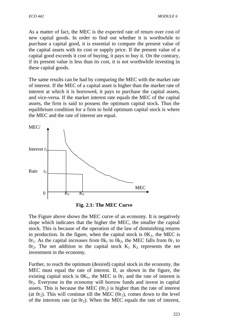
ECO 442 MODULE 6
223
As a matter of fact, the MEC is the expected rate of return over cost of
new capital goods. In order to find out whether it is worthwhile to
purchase a capital good, it is essential to compare the present value of
the capital assets with its cost or supply price. If the present value of a
capital good exceeds it cost of buying, it pays to buy it. On the contrary,
if its present value is less than its cost, it is not worthwhile investing in
these capital goods.
The same results can be had by comparing the MEC with the market rate
of interest. If the MEC of a capital asset is higher than the market rate of
interest at which it is borrowed, it pays to purchase the capital assets,
and vice-versa. If the market interest rate equals the MEC of the capital
assets, the firm is said to possess the optimum capital stock. Thus the
equilibrium condition for a firm to hold optimum capital stock is where
the MEC and the rate of interest are equal.
MEC/
Interest r1
Rate r2
MEC
0 K1 K2
Fig. 2.1: The MEC Curve
The Figure above shows the MEC curve of an economy. It is negatively
slope which indicates that the higher the MEC, the smaller the capital
stock. This is because of the operation of the law of diminishing returns
in production. In the figure, when the capital stock is 0K1, the MEC is
0r1. As the capital increases from 0k1 to 0k2, the MEC falls from 0r1 to
0r2. The net addition to the capital stock K1 K2 represents the net
investment in the economy.
Further, to reach the optimum (desired) capital stock in the economy, the
MEC must equal the rate of interest. If, as shown in the figure, the
existing capital stock is 0K1, the MEC is 0r1 and the rate of interest is
0r2. Everyone in the economy will borrow funds and invest in capital
assets. This is because the MEC (0r1) is higher than the rate of interest
(at 0r2). This will continue till the MEC (0r1), comes down to the level
of the interests rate (at 0r2). When the MEC equals the rate of interest,

ECO 442 ADVANCED MACROECONOMICS
224
the economy reaches the level of optimum capital stock. The fall in the
MEC is due to the increase in the actual capital stock from 0K1 to the
optimum (desired) capital stock 0K2. The increase in the economy’s
capital stock by K1 K2 is the net investment of the economy. But it is the
rate of interest which determines the size of the optimum capital stock in
the economy. And it is the MEC which relates the amount of desired
capital stock to the rate of interest. Thus, the negative slope of the MEC
curve indicates that as the rate of interest falls, the optimum stock of
capital increases.
The marginal efficiency of investment (MEI): The MEI is the rate of
return expected from a given investment on a capital asset after covering
all it costs, except the rate of interest. Like the MEC, it is the rate which
equates the supply price of a capital asset to its prospective yield. The
investment on an asset will be made depending upon the interest rate
involved in getting funds from the market. If the rate of interest is
higher, investment is at a low level. A low rate of interest leads to an
increase in investment. Thus, the MEI relates the investment to the rate
of interest. The MEI schedule shows the amount of investment
demanded at various rates of interest. That is why; it is also called the
investment demand schedule or curve which has negative slope as
shown in Figure 3.4 below:
Fig. 2.2: The MEI Schedule

ECO 442 MODULE 6
225
At 0r1 rate of interest, investment is 0I1. As the rate of interest falls to
0r2, investment increases to 0I1I
(panel A). To what extend the fall in
interest rate will increase investment depends upon the elasticity of
investment demand curve of the MEI curve. The less elastic is the MEI
curve, the lower is the increase in investment as result of fall in the rate
of interest, and vice versa .
In Figure 3.4, the vertical axis measures the amount of investment; the
MEI and MEII are the investment demand curves. The MEI curve is
panel (A) is less elastic, so investment increases by III
II which is less
than the increase in investment I1I2 shown in panel (B) where the MEII
curve is elastic.
Shortcomings of the marginal efficiency theory
(1) It does not give explicit recognition to the role of expectations in
investment decisions making. Yet the role of expectation is
important in an attempt to capture an investor’s view about the
probability distribution of the possible stream of returns
(2) Eisner and Strotz (1963) argued that the determinant of the
internal rate of return that is used in discounting the stream of
returns to their present value equivalent is both subjective and
ambiguous. This criticism is of particular relevance in
underdeveloped economies characterised by underdeveloped and
imperfect capital market.
(3) The concept of the “market rate of interest” is questionable. This
is because what exists in practice and especially within the
context of underdeveloped capital market is not the “market rate
of interest” but a series of interest rates namely Lending rate,
Minimum Rediscount Rate, Treasury Bill Rate etc. The difficulty
of accepting any of these rates as optimal in the context of
deregulation of interest rate as we have in Nigeria is even more
fundamental. It is in cognisance of this that Ott, et al. (1975)
caution that investors exercise cares in selecting the rate of
interest they compare to MEI.
SELF-ASSESSMENT EXERCISE
Explain the marginal efficiency theory and the shortcomings therein.

ECO 442 ADVANCED MACROECONOMICS
226
3.3 Relationship between the MEC (Capital stock) and the
MEI (Investment)
Professor Lerner pointed out as early as in 1946 that Keynes erred not
only descriptively but also analytically by failure to distinguish between
the marginal efficiency of capital (MEC) and the marginal efficiency of
investment (MEI). Following Lerner, Gardner Ackley and some other
economists have clearly defined and distinguished between the two
concepts.
The MEC is based on a given supply price for capital, and the MEI on
induced changes in the price. The MEC shows the rate of return on all
successive units of capital without regard to the existing stock of capital.
On the other hand, the MEI shows the rate of return on only units of
capital over and above the existing stock of capital. The MEC
determines the optimum capital stock in an economy at each level of
interest rate. The MEI determines the net investment of the economy at
each interest rate, given the stock of capital.
In the words of Anyanwu (1995), the distinction between MEC and MEI
can be illustrated graphically as shown in Figure 2.3. The distinction
between both concepts has been summarised by Shapiro (1974) as
follows: “ a MEC schedule (curve) is constructed holding constant the
supply cost of new capital and the expected rate of return on future cash
flow.
%
Interest 10
Rate 5
3
MEI MEC
0 I
Fig. 2.3: Marginal Efficiency of Investment and Marginal
Efficiency of Capital
The MEI schedule (curve) also holds the expected rate of return of
future cash flows constant but assumes that the supply cost of new
capital is positively related to the production of new capital. Since the
ECO 442 MODULE 6
227
expected rate of return from investment proposals fall as the supply cost
of new capital rises, the MEI schedule (curve) has a steeper slope and is
to the left of the MEC schedule as illustrated above.
SELF-ASSESSMENT EXERCISE
i. Explain the relationship between the Marginal Efficiency of
Capital (MEC) and the Marginal Efficiency of Investment (MEI).
ii. Differentiate between the MEC and the MEI.
4.0 CONCLUSION
The main concern of this unit has been essentially with the theories of
investment: The accelerator and the marginal efficiency theories. We
have also looked at the three elements that show the relationships of the
businessman’s estimate of the profit or loss that will accrue from any
particular investment. These elements are: the expected income flow
from the capital good in question, the purchases price of that good, and
the market rate of interest. The determinants of inducement to invest are
a number of factors other than interest rate which affect the inducement
to invest.
5.0 SUMMARY
So far in this unit, we have attempted to explain the various theories of
investment. Net investment expenditures for anytime period, are the
means by which a change in the capital stock is affected. Net
investment, which is zero when the actual capital stock equals the profit
maximising capital stock, becomes positive when the profit maximising
stock exceeds the actual stock. A prerequisite to the appearance of net
investment expenditure is a rise in the profit-minimising capital stock
whether such a difference will appear depends on the relationship
between the MEC schedule and the market rate of interest. The MEC in
turn depends on the cost price of capital goods and the expected rate of
return from such goods.
We also noted that the rate of net investment expenditures depends on
the relationship between the rate of interest and the MEI schedule. The
overall slope of the MEI schedule depends in turn on the cost price of
capital goods and that its positions vis-à-vis the axes depends on the
actual stock of capital. This is summarised in Figure 2.4.

ECO 442 ADVANCED MACROECONOMICS
228
Capital Stock Expenditure income flow from
capital goods
MEC Schedule Market rate of interest Profit maximizing Actual
Capital Stock
Capital Stock
Rate of Net Investment
Expenditures
MEI Schedule Market Rate of Interest
Slope: Supply price Position; Actual
of Capital Goods Capital stock
Fig. 2.4: From the Stock of Capital to the Rate of Investment
6.0 TUTOR-MARKED ASSIGNMENT
1. Distinguish carefully between MEC and MEI; hence discuss
Keynes’ marginal efficiency theory of investment as well as the
shortcomings of the theory.
2. Explain the accelerator hypothesis and the derivation of the
accelerator model.
7.0 REFERENCES/FURTHER READING
Anyanwu, J.C. (1995). Modern Macroeconomics: Theory and
Applications in Nigeria. Nigeria: Joanee Educational Publishers
Limited.
Eisner, R.A. & Stortz, R.H. (1963). “Determinants of Business
Investments: Impact of Monetary Policy.” Commission on Money
and Credit.
Eisner, R.A. & Nadir, M.I. (1968). “Investment Behaviour and
Neoclassical Theory.” Review of Economic Policy. Vol. 50.
Shapiro, E. (1974). Macroeconomic Analysis. (3rd ed.). New York:
Harcourt Brace Jovanovich, Inc.

ECO 442 MODULE 6
229
UNIT 3 INVESTMENT DEMAND: THE RATE OF
INTEREST AND THE ROLE OF FINANCE
CONTENTS
1.0 Introduction
2.0 Objectives
3.0 Main Content
3.1 Determinants of the Elasticity of the MEC Schedule
3.2 The Role of Finance, Beyond the Rate of Interest
3.3 Factors other than Interest Rate Affecting Inducement to
Invest
4.0 Conclusion
5.0 Summary
6.0 Tutor-Marked Assignment
7.0 References/Further Reading
1.0 INTRODUCTION
The extent to which a change in the rate of interest causes a change in
the rate of investment spending depends on the elasticity of the MEC
schedule. The more elastic the schedule, the greater the increase or
decrease in the profit-maximising capital stock that follows from any
decrease or increase in the rate of interest. In order to specify the
relationship between a change in the rate of interest and a change in the
rate of investment spending, we must proceed from a change in the rate
of interest through the resultant change in the profit-maximising capital
stock to the resultant change in the rate of investment.
2.0 OBJECTIVES
At the end of this unit, you should be able to:
explain the determinant of the elasticity of the MEC schedule
describe the role of finance, beyond the rate of interest
discuss the factors other than interest rate affecting inducement to
invest.
3.0 MAIN CONTENT
3.1 The Determinant of the Elasticity of the MEC Schedule
Assuming again that a firm buys capital goods only in the expectation
that each purchase will add to its profits, the elasticity of the MEC
schedule for the economy as a whole may be said to depend on the

ECO 442 ADVANCED MACROECONOMICS
230
significance of any given change in the interest rate as a factor altering
the profit-maximising or desired capital stock for all firms combined. A
fall in the interest rate may lead some firms to expand their stock of
capital goods substantially, while the same fall in the interest rate may
lead other firms to no expansion at all. The elasticity of the aggregate
MEC schedule thus depends on the combined responses of all firms to
any change in the interest rate.
Fig. 3.1: Net Investment with an Inelastic Marginal Efficiency
of Capital Schedule
Our problem, then, is to investigate what determines whether any given
change in the interest rate will lead to a larger or smaller change in the
profit-maximising capital stock. Although it is immediately apparent
that a lower interest rate, other things being equal, is also a reduction in
one cost of doing business, we find that different businesses respond
differently to such a drop. In seeking an explanation for this disparate
reaction, we will get at the factors that determine the elasticity of the
MEC schedule.
With all other things assumed to remain unchanged, especially the
existing state of technology, one factor that determines how great an
increase in the profit-maximising capital stock will result from any
given reduction in the interest rate is the extent to which firms find it
technologically possible to substitute what is now the relatively more
expensive labour input. It must be seen here that, in terms of the cost of
factor units, the comparison is between the rate of interest as the cost of
capital and wage rate as the cost of labour. Since we express the rate of
return from or the productivity of an addition to the stock of capital as a
percentage – namely, the MEC – we must for comparability express the
cost of capital as another percentage – namely, the market rate of
interest. A fall in the rate of interest is then a decrease in the cost of
capital. In contrast, since we express the return from or the productivity
of an addition of a unit of a given type of labour as the naira value of the

ECO 442 MODULE 6
231
output that will be produced because of that additional unit, the cost of
labour is also expressed as a naira value, the naira cost of a unit of the
given type of the labour. A fall in the wage rate paid labour is then a
decrease in the cost of labour.
With a fall in the interest rate and no change in the wage rate, there will
be a tendency throughout the economy to substitute the cheaper input,
capital, for the more expensive input, labour, in the production of any
constant level of output. Although such a tendency will be present
throughout the economy, the extent to which substitution of this sort
actually takes place will vary widely from industry to industry and , to a
lesser extent, from firm to firm.
SELF-ASSESSMENT EXERCISE
Discuss extensively the determinant of the elasticity of the MEC
schedule.
3.2 The Role of Finance, Beyond the Rate of Interest
So far in this chapter, the role of finance in the investment decision has
been drastically simplified by assuming that it involves only one
element, the market rate of interest. Investment spending in any time
period has been determined from the MEI schedule by drawing a
horizontal line at the market rate of interest to an intersection with the
MEI schedule. With a given MEI schedule, only a change in the rate of
interest would produce a change in investment demand.
Without denying the underlying correctness of this basic relationship,
we must recognise the oversimplification that it involves. By showing
that aggregate investment spending is determined by the intersection of
the MEI curve with a horizontal line drawn at the prevailing rate of
interest, we are assuming for one thing that funds are available in
unlimited amounts to borrowers of every description at this one
particular rate of interest that we called market rate of interest. A first
objection to this is the fact that, in reality, there is no such thing as the
market rate of interest. Rather there is a whole complex of rates. The
rate paid by any particular borrower depends on such variables as the
term of the loan, the size of the loan, the collateral offered, and
especially the credit worthiness of the borrower. Beyond this, there is
not an unlimited supply of funds available to any single borrower in any
time period at this rate; there is some tendency for the rate he pays to
rise with each addition to his indebtedness per time period, other things
being equal.

ECO 442 ADVANCED MACROECONOMICS
232
A more fundamental objection to this formulation is its implication that
the only way in which firms may secure funds to finance investment
spending is by borrowing in the market and paying whatever rate of
interest they must pay. Actually there are three sources of funds for
investment, only one of which involves borrowing in the usual sense of
that word. These are (1) undistributed profits and depreciation
allowances or so-called internal funds, (2) borrowing from the banks or
in the bond market, the source usually thought of in connection with the
market rate of interest, and (3) equity financing or the sale of new stock
issues. There are different costs and different risks incurred by firm in
using each of these sources, but the cost of funds from each may still be
expressed as a percentage so that one is compared with the other.
SELF-ASESSMENT EXERCISE
Explain the role of finance in investment decision.
3.3 Factors Other than Interest Rate Affecting Inducement
to Invest
There are a number of factors other than the rate of interest which affect
the inducement to invest. They are the following:
(1) Element of uncertainty. According to Keynes, the MEC is more
volatile than the rate of interest. This is because the prospective
yield of capital assets depends upon the business expectations.
These business expectations are very uncertain. “They may
change quickly and drastically in response to the general mood of
the business community, rumors, news of technical
developments, political events, even directors’ ulcers may cause a
sudden rise or fall of the expected rate of yield. As a result, it is
difficult to calculate the expected annual returns on the life of a
capital asset. As Keynes himself wrote, “if we speak frankly we
have to admit that our basis of knowledge for estimating the yield
ten years hence of a railway, a copper mine, a textile factory, the
goodwill of a patent medicine, an Atlantic liner, a building in the
city of London amounts to little and sometimes nothing; or even
five years hence”. Further, because of uncertainty, investment
projects usually have a short pay-off period. Capital assets
become obsolete earlier than their expected life due to rapid
technological developments. The rate of depreciation also does
not remain constant and varies much. So firms have a tendency to
invest only if they are in a position to recover the capital outlay in
a short period. These factors tend to bring instability in the
investment function.

ECO 442 MODULE 6
233
(2) Existing stock of capital goods. If the existing stock of capital
goods is large, it would discourage potential investors from
entering into the making of goods. Again, the induced investment
will not take place if there is excess or idle capacity in the
existing stock of capital assets. In case the existing stock of
machines is working to its full capacity, an increase in the
demand for capital goods manufactured by them will raise the
demand for capital goods of this type and raise the inducement to
invest. But it is the capital stock which influences the MEC. The
MEC and the capital stock are inversely related.
(3) Level of income. If the level of income rises in the economy
through rise in money wage rates and other factors prices, the
demand for goods will rise which will, in turn, raise the
inducement to invest. Contrariwise, the inducement to investment
will fall with the lowering of income levels.
(4) Consumer demand. The present and future demand for the
products greatly influences the level of investment in the
economy. If the current demand for consumer goods is increasing
rapidly, more investment will be made. Even if we take the future
demand for the products, it will be considerably influenced by
their current demand and both will influence the level of
investment. Investment will be low if the demand is low, and vice
versa.
(5) Liquid assets. The amounts of liquid assets with the investors
also influence the inducement to invest. If they possess large
liquid assets, the inducement to invest is high. This is especially
the case with those firms which keep large reserve funds and
undistributed profits. On the contrary, the inducement to invest is
low for investors having little liquid assets.
(6) Inventions and innovations. Inventions and innovations tend to
raise the inducement to invest. If inventions and technological
improvements lead to more efficient methods of production
which reduce costs, the MEC of new capital assets will rise.
Higher MEC will induce firms to make larger investments in the
new capital assets and in related ones. The absence of new
technologies will mean low inducement to invest. An innovation
also includes the opening of new areas. This requires the
development of means of transport, the construction of housing
etc, leading to new investment opportunities. Thus inducement to
invest rises.

ECO 442 ADVANCED MACROECONOMICS
234
(7) New products. The nature of new products in terms of sales and
costs may also influence their MEC and hence investment. If the
sale prospects of a new product are high and the expected
revenues more than the costs, the MEC will be high which will
encourage investment in this and related industries. For example,
the invention of television must have encouraged the electronics
industry to invest in these capital assets and used them to produce
television sets, if they had expected profits to be higher than
costs. Thus lower maintenance and operating costs in the case of
new products are important in increasing the inducement to invest
(8) Growth of population. A rapid growing population means a
growing market for all types of goods in the economy. To meet
the demand of an increasing population in all brackets,
investment will increase in all types of consumer goods
industries. On the other hand, a declining population results in a
shrinking market for goods thereby lowering the inducement to
invest.
SELF-ASSESSMENT EXERCISE
What do you mean by induced investment? Discuss the determinants of
inducement to invest.
4.0 CONCLUSION
In the previous unit, we worked our way through the pure mechanics of
the process by which changes in the profit maximising or desired capital
stock are translated into changes in the rate of investment spending. We
saw how the profits and the accelerator theories explain changes in the
desired capital stock, and in the first part of this unit, we looked at the
way a change in the rate of interest does the same thing.
Whatever may have brought it about; a divergence in which the desired
capital stock exceeds the actual capital stock will cause a right-ward
shift in the MEI curve. The greater the shift, the greater will be the rate
of net investment spending. Once we have explained the shift in the MEI
curve, we need look no further if we assume that the supply of funds
available prevailing market rate of interest.
5.0 SUMMARY
This unit examined the determinant of elasticity of the MEC schedule to
include the extent to which firms find it technologically possible to
substitute what is now the relatively more expensive labour input. The
unit also looked at the role of finance beyond the rate of interest. The

ECO 442 MODULE 6
235
unit equally discussed a number of factors other than the rate of interest
which affect the inducement to invest.
6.0 TUTOR-MARKED ASSIGNMENT
While the MEC determines the optimum capital stock in an economy at
each level of interest rate the MEI determines the net investment of the
economy at each interest rate, given the capital stock. Discuss.
7.0 REFERENCES/FURTHER READING
Anynawu, J.C. (1995). Modern Macroeconomics: Theory and
Applications in Nigeria. Nigeria: Joanee Educational Publishers
Limited.
Shapiro, E. (1974). Macroeconomic Analysis. (3rd ed.). New York:
Harcourt Brace Jovanovich, Inc.

ECO 442 ADVANCED MACROECONOMICS
236
MODULE 4 THE IS-LM FRAMEWORK
Unit 1 The Product Market Equilibrium and the IS Curve
Unit 2 The Money Market Equilibrium and the LM Curve
Unit 3 General Equilibrium Analysis of Product and Money
Market
UNIT 1 THE PRODUCT MARKET EQUILIBRIUM AND
THE IS CURVE
CONTENTS
1.0 Introduction
2.0 Objectives
3.0 Main Content
3.1 The Product or Goods Market Equilibrium
3.2 The IS Curve
3.2.1 Derivation of the IS Curve
3.3 The Slope of the IS Curve
3.4 Shift in the IS Curve
4.0 Conclusion
5.0 Summary
6.0 Tutor-Marked Assignment
7.0 References/Further Reading
1.0 INTRODUCTION
Our general model in this unit is the determinants of equilibrium in the
market for goods and the derivation of the IS curve. The IS - is the
shorthand expression of the equality of investment and saving which
represents the product market equilibrium. The understanding of this
unit and the subsequent unit gives you a broader knowledge of how the
various policies of fiscal and monetary work are stabilising an economy.
Hence you need to pay adequate attention.
2.0 OBJECTIVES
At the end of this unit, you should be able to:
explain equilibrium in the goods or product market
discuss the equality of savings and investment
describe algebraically and graphically the IS curve
explain the slope of IS as well as shift in IS curve.

ECO 442 MODULE 6
237
3.0 MAIN CONTENT
3.1 The Product or Goods Market Equilibrium
The goods or products market equilibrium is defined by equality
between saving (S) and investment (I) - the condition that gave us the
equilibrium level of income. At the level of income at which S = I (a
simple two-sector economy), the leakage from the income stream into
saving is exactly matched by offsetting investment spending; or at this
income level, aggregate demands for goods just equals the aggregate
supply of goods. There is, accordingly, goods market equilibrium at this
level of income (Shapiro, 1974).
The product market is in equilibrium when desired savings and
investment are equal. Saving is a direct function of the level of income.
S = s(Y)……………………………………………….. ... (4.1)
Investment is a decreasing function of interest rate,
I = I(r)……………………………………………………... (4.2)
From equation (4.1) and (4.2), we have S = I
Equilibrium condition is s (Y) = I(r)………………………………. (4.3)
It is also assumed in the presents analysis that the price level is stable so
that all changes in saving, investment and income (and in the interest
rate as well) are real changes.
The set of equations maybe shown graphically as in Figure 1.1 below:
Part A gives the MEI (investment demand) schedule, showing that
investment spending varies inversely with the interest rate. The straight
line in part B is drawn at an angle 450 from the origin. Whatever the
amount of planned investment measures along the horizontal axis of part
B, equilibrium requires that planned saving measured along the vertical
axis of part B be the same. Thus, all points along the 450 line in part B
indicate equality of saving and investment. Part C brings in the saving
function, showing that saving varies directly with income.

ECO 442 ADVANCED MACROECONOMICS
238
Fig. 1.1: Goods Market Equilibrium
SELF-ASSESSMENT EXERCISE
Explain the product market equilibrium.
3.5 The IS Curve
The IS curve or schedule reflects the equilibrium of the product market.
It is the locus of pairs of income and interest rate for which the
expenditure sector is at equilibrium. That is, the expenditure (or goods)
market equilibrium curve or IS curve shows combination of interest
rates and levels of output such that planed spending equals income. It is
that relationship that links the level of income and the interest rate such
that investment demands plus government demand equals saving plus
taxes.
I + G = S + T. Equivalently, the IS curve is the relationship between the
level of income and interest rate which ensures that aggregate demand
(consumption demand plus investment demand plus government
demand ) is equal to the level of income:

ECO 442 MODULE 6
239
Y = C + I + G or
Y = α + βy + I0 + I1 (Y, r)…………………………… (4.4)
Thus, there exist a set of combinations for Y and r which provide
equilibrium in the expenditure market, by equating expenditure plans
with income. By implication those sets of Y and r also equate the
planned levels of saving and investment that is satisfying the condition:
S = I or S0 + S1 (Y) = I0 + I1 (Y, r)……………………… (4.5)
3.2.1 Derivation of the IS Curve.
The IS curve which is negatively sloped can be derived as shown in
Figure 1.1 above.
Quadrant (A) Part A shows the relationship between investment and
interest rate hence yielding the marginal efficiency of investment
(MEI).
Quadrant (B) Part B shows the saving–investment equality i.e. the
demonstration of the equality of planned saving and planned investment.
Quadrant (C) Part C shows the saving schedule where savings are
positively related to income.
Quadrant (D) Part D of the figure is the goods market equilibrium,
yielding the IS curve.
Algebraically the IS curve can be derived from the following
procedures:
Let’s assume that income is made up of only consumption and
investment, where investment is dependent on income and interest rate.
Y = C + I
C = α + βY
I = I0 + I1Y – I2r
We then solve for the endogenous variable, Y in terms of the exogenous
variables r
Y = α + βY + I0 + I1Y – I2r…………………………… (4.6)
Y = 1/1 – β – I1 [α + I0 - I2r]…………………………… (4.7)
This expresses the equilibrium level of income as a function of the rate
of interest and it is referred to as the IS curve when shown graphically.

ECO 442 ADVANCED MACROECONOMICS
240
SELF-ASSESSMENT EXERCISE
What do you understand by the “IS curve”? Draw the IS curve both
graphically and algebraically.
3.5 The Slope of the IS Curve
The IS curve slopes downward from left to right. This negative slope
reflects the increase in investment and income as the rate of interest
falls. The IS curve may be flat or steep depending on the sensitiveness
of investment to changes in the rate of interest, and also on the size of
the multiplier (1/1 – β – I1).
If investment is very sensitive to the rate of interest, the IS curve is very
flat. This is shown by the segment AB of the IS curve in Figure 1.2
where a fall in the rate of interest from r1 to r2 leads to a proportionate
large rise in income from Y1 to Y2. The IS curve is interest elastic in the
AB segment of the IS curve.
On the other hand, if investment is not very sensitive to the rate of
interest, the IS curve is relatively steep in terms of Figure 1.2, when the
rate of interest falls from r2 to r3, income increases by a relatively
smaller amount Y2 Y3.
Fig. 1.2: The Slope of IS curve
The BC segment of the IS curve is less interest elastic. Any further fall
in the rate of interest from r3 will led to no change in income because the
IS curve is vertical in that range. It is interest inelastic. Algebraically,
the negative slope of the IS curve can be obtained by taking the partial
derivative of income, Y with respect to interest rate r of equation (4.7):
Y = 1/1 – β – I1 [α + I0 - I2r]
dY/dr = -I2/1 – β – I1 < 0………………………………….(4.8)

ECO 442 MODULE 6
241
SELF-ASSESSMENT EXERCISE
Discuss why the slope of IS curve is negative.
3.5 Shifts in the IS Curve
The IS functions shifts to the right with a reduction in saving. Reduction
in saving may be the result of one or more factors leading to increase in
consumption or increase in investment. Moreover, government
expenditure and tax policies have the effect of shifting the IS function.
In all these cases, the IS function will shift to the right, equal to the
decrease in the supply of saving times the multiplier or the increase in
the investment times the multiplier. With the increase in the autonomous
investment, the IS curve shifts from IS1 to IS2 and the new equilibrium
is established at point E2 which indicates a higher level of income Y2 at
a higher interest rate, as shown in Figure 1.3 below:
r
E2
E1 IS2
IS1
0 Incomes
Fig. 1.3: Shifts in the IS Curve
In the opposite case, when investment falls or saving increases, the IS
function will shift to the left and the equilibrium will be established at a
lower level of income and interest rate. This situation can be explained
by assuming IS2 as the original curve.
SELF-ASSESSMENT EXERCISE
Discuss the factors that can led to a shift in the IS function.
4.0 CONCLUSION
You have seen from the analysis that the basic concept of the product
market equilibrium is essential for the derivation of the IS curve.
ECO 442 ADVANCED MACROECONOMICS
242
Equality of saving and investment is the basic element of equilibrium in
the real sector or product market. Therefore it has been argued that the
IS curve or function is the locus of pairs of interest rate and levels of
income where the goods or the product market is in equilibrium.
5.0 SUMMARY
This unit has explained the product market and the derivation of the IS
curve. Both the graphical and the algebraic derivation of the IS functions
(curve) have been considered alongside the slope and shifts in the IS
curve. In the next unit, you will be introduced to the money market and
the LM curve.
6.0 TUTOR-MARKED ASSIGNMENT
1. Graphically and algebraically derive the IS functions including
the slope of the IS curve.
2. What are causes of shifts in the IS curve?
7.0 REFERENCES/FURTHER READING
Anyanwu, J.C. & Oaikhenan, H.E. (1995). Modern Macroeconomics:
Theory and Applications in Nigeria. Onitsha-Nigeria: Joanee
Educational Publishers Limited.
Dornbusch, R., Fischer, S. & Startz, R. (2008). Macroeconomics. (10th
ed.). New York: MacGraw- Hill/Irwin.
Parkin, M. (1982). Modern Macroeconomics. Ontario: Prentice-Hall,
Canada Inc.
Shapiro, E. (1974). Macroeconomic Analysis. (3rd ed.). New York:
Harcourt Brace Jovanovich, Inc.

ECO 442 MODULE 6
243
UNIT 2 MONEY MARKET EQUILIBRIUM AND THE
LM CURVE
CONTENTS
1.0 Introduction
2.0 Objectives
3.0 Main Content
3.1 The Money Market Equilibrium
3.2 The LM Curve
3.2.1 Derivation of the LM Curve
3.3 The Slope of the LM Curve
3.4 Shifts in the LM Curve
4.0 Conclusion
5.0 Summary
6.0 Tutor-Marked Assignment
7.0 References/Further Reading
1.0 INTRODUCTION
The term LM is the short hand expression of the equality of money
demand (L) and money supply (M) and represents the money market
equilibrium. Just as the IS function which represents equilibrium in the
goods market where saving equals investment, the understanding of the
LM concept helps you to also have a broader knowledge of how
monetary policy works in an economy hence the need to pay adequate
attention.
2.0 OBJECTIVES
At the end of this unit, you should be able to:
explain equilibrium in the money market
analyse the equality of demand for and supply of money
illustrate both graphically and algebraically the LM function
explain the slope as well as the shift in LM curve.
3.0 MAIN CONTENT
3.1 The Money Market Equilibrium
Equilibrium in the money market requires equality between the supply
of and the demand for money. The Keynesian theory of the demand for
money makes the transactions demand (which is here combined with the
precautionary demand), a direct function of the income level alone, or

ECO 442 ADVANCED MACROECONOMICS
244
Lt = k(Y)……………………………………………………..(4.9)
and the speculative demand, an inverse function of the interest rate
alone, or
Ls = I (r)…………………………………………………… (4.10)
Total demand for money is:
L = LT + Ls = k(Y) + I(r)…………………………………. (4.11)
The supply of money M is determined outside the model - it is
exogenous. This may be written as
M = M0…………………………………………………… (4.12),
In which M0 is simply the amount of money that exists, an amount
determined by the monetary authorities. This gives us three equations to
cover the money market:
Demand for money LT + Ls = k(Y) + I(r)
Supply of money M = M0
Equilibrium condition L = M
As before, it is assumed that prices are stable, so that a change in any
variable is entirely a real change.
This set of equations is shown graphically in Figure 2.1. Part A shows
the speculative demand for money as a function of ‘r’. Part B is drawn to
show a total money supply, all of which must be held in either
transaction balances (LT) or speculative balances (LS). The points along
the line indicate all the possible ways in which the given money supply
may be divided between LT and LS. Part C shows the amount of money
required for transactions purposes at each level of income. The LM
curve of part D is derived from the other parts.

ECO 442 MODULE 6
245
Fig. 2.1: Money Market Equilibrium
SELF-ASSESSMENT EXERCISE
Explain the money market equilibrium.
3.2. The LM Curve
The LM curve shows all the combinations of interest rate and levels of
income at which the demand for and supply of money are equal. In other
words, the LM schedule shows the combinations of interest rates and
levels of income where the demand for money (L) and the supply of
money (M) are equal such that the money market is in equilibrium.
The LM curve is derived from the Keynesian formulation of liquidity
preference schedule and the schedule of money. The LM curve is
positively sloped such that an increase in the interest rate reduces the
demand for real balances. To maintain the demand for real balances
equal to the fixed money supply, the level of income has to rise in the
same vein; money market equilibrium implies an increase in the interest
rate is accompanied by an increase in the level of income (Dormbusch &
Fischer, 1974).

ECO 442 ADVANCED MACROECONOMICS
246
3.2.1 Derivation of the LM Curve
Graphically, the LM curve can be derived as shown in Figure 2.2 below:
Quadrant A Here, the speculative demand for money in relation to
interest rate is shown as a negatively sloping curve.
Quadrant B In this quadrant, the total money supply is shown as a
negatively sloping Curve.
Quadrant C The transactions demand for money in relations to income
is here shown as a positively sloping curve.
Quadrant D The money market is demonstrated as the equality between
money demand and money supply and hence yielding the LM curve.
Assume in part A, an interest rate of (r2); at this interest rate the public
will want to hold Ls1 in speculative balances. In part B, subtracting the
Ls1 of speculative balances from the total money supply leaves Lt2 of
transactions balances, an amount consistent with an income of level of
Y2 as shown in part C. Finally, in part D, bringing together Y2 from Part
C and r2 from part A, we have one combination of Y and r at which L =
M or at which there is equilibrium in the market for money. If we
assume the lower interest rate of r1, part A indicates that speculative
balances will be Ls2; Part B indicates that transaction balances will be
LT1 and part C indicates the income level of Y1 as that is consistent with
the transaction balances of LT1. This gives us another combination of Y
and r at which L = M. Other such combinations can be determined in the
same way. The function in part D labeled LM results when these
combinations are connected.
Algebraically, for the money market to be in equilibrium, we require
that money demand equals money supply.
M = L or
M = L0 + L1Y – L2r ……………………..……………… (4.13)
Such that solving for r in terms of Y gives us:
r = 1/L2 [L0 + L1Y – M]…………………………………. (4.14)
This equation expresses the equilibrium rate of interest as a function of
the level of income and its graph is called LM curve as shown in Figure
2.1.

ECO 442 MODULE 6
247
SELF-ASSESSMENT EXERCISE
i. What do you understand by the LM curve?
ii. Illustrate the LM function both graphically and algebraically.
3.3 The Slope of the LM Curve
The LM curve slopes upward from left to right because given the supply
of money, an increase in the level of income, increases the demand for
money which leads to higher rate of interest. This, in turn, reduces the
demand for money and thus keeps the demand for money equal to
supply of money. The smaller the responsiveness of the demand for
money to income, and the larger the responsiveness of the demand for
money to the rate of interest, the flatter will be the LM curve. This
means that a given change in income has a smaller effect on the interest
rate.
The LM curve is steeper, if a given change in income has a larger effect
on the rate of interest. In this situation, the responsiveness of the demand
for money to income is larger and is smaller for the interest rate. If the
demand for money is insensitive to interest rate, the LM curve is
vertical, that is perfectly inelastic. If the demand for money is very
sensitive to the rate of interest, the LM curve is horizontal. The LM
curve is perfectly elastic in relation to the rate of interest. This portion of
the LM curve at the extreme left is equivalent to the Keynesian liquidity
trap.
Algebraically, the positive slope of the LM curve can be obtained by
taking the partial derivative of the LM curve i.e. r with respect to Y.
r = 1/L2 [-M + L0 + L1Y]…………………………………..(4.15)
dr/dY = L1/L2……………………………………………….(4.16)
SELF-ASSESSMENT EXERCISE
Discuss the reason why the slope of the LM curve is positive.
3.3 Shifts in the LM Curve
The LM function shifts to the right with the increase in the money
supply given the demand for money, or due to the decrease in the
demand for money, given the supply of money. If the Central bank
follows an expansionary monetary policy, it will buy securities in the
open market. As a result, money supply with the public increases for
both transaction and speculative purposes. This shifts the LM curve to
the right.

ECO 442 ADVANCED MACROECONOMICS
248
A decrease in the demand for money means a reduction in the quantity
of balances demanded at each level of income and interest rate. Such a
decrease in the demand for money balances creates an excess of the
money supplied over the money demanded. This is equivalent to an
increase in money supply in the economy which has the effect of
shifting the LM curve to the right.
Fig. 2.2: Shift in the LM Curve
With the increase in the money supply, the LM curve shifts to the right
as LM2 which moves the economy to a new equilibrium point E2. The
increase in the money supply brings down the interest rate to r2 in the
money market. This, in turn, increases investment thereby raising the
level of income to Y2.
Thus, the effect of the increase in money supply is to shift the LM curve
to the right and a new equilibrium is established at a lower interest rate
r2 and higher income level Y2.
Contrariwise, a decrease in the money supply or an increase in the
demand for money will shift the LM curve/function to the left such that
a new equilibrium is established at a higher interest rate and lower
income level. This case can be explained by assuming LM2 as the
original curve.
SELF-ASSESSMENT EXERCISE
Discuss the factors that can lead to shifts in the LM curve.
4.0 CONCLUSION
So far this unit has thrown light, that the basic concept of the money
market equilibrium is essential for the derivation of the LM curve.
Equality of the demand for money and the supply of money is the basic
element in the money market equilibrium. Therefore, it has been argued

ECO 442 MODULE 6
249
that the LM curve is the locus of pairs of interest rate and levels of
income where the demand for money (L) equals the supply of money
(M).
5.0 SUMMARY
Discussion on the money market and the derivation of the LM curve has
been done. Both graphical and algebraic derivation of the LM curve has
been considered, alongside the slope and shifts in the LM curve. The
slope of the LM curve has been shown to be positive while a shift in the
LM curve is caused by an increase or decrease in money supply as well
as a decrease or increase in the demand for money.
6.0 TUTOR-MARKED ASSIGNMENT
1. Graphically and algebraically derive the LM function including
the slope of the function.
2. What are the causes of shifts in the LM curve?
7.0 REFERENCES/FURTHER READING
Anyanwu, J.C. & Oaikhenan, H.E. (1995). Modern Macroeconomics:
Theory and Applications in Nigeria. Onitsha-Nigeria: Joanee
Educational Publishers Limited.
Dornbusch, R., Fischer, S. & Startz, R. (2008). Macroeconomics. (10th
ed.). New York: MacGraw- Hill/Irwin.
Jhinghan, M.L. (2003). Macro-Economic Theory. (11th ed.). VRINDA
Publications (P) Limited.
Shapiro, E. (1974). Macroeconomic Analysis. (3rd ed.). New York:
Harcourt Brace Jovanovich, Inc.

ECO 442 ADVANCED MACROECONOMICS
250
UNIT 3 GENERAL EQUILIBRIUM OF PRODUCT AND
MONEY MARKET (IS-LM FRAMEWORK)
CONTENTS
1.0 Introduction
2.0 Objectives
3.0 Main Content
3.1 Meaning of IS-LM Framework and the General
Equilibrium
3.2 A Change in Investment/Government Spending (Fiscal
Policy)
3.3 A Change in Money Supply (Monetary Policy)
3.4 A Simultaneous Change in Investment and Money Supply
(Fiscal-Monetary Policy Mix)
4.0 Conclusion
5.0 Summary
6.0 Tutor-Marked Assignment
7.0 References/Further Reading
1.0 INTRODUCTION
So far we have analysed the conditions that have to be satisfied for the
general equilibrium of the product and money markets in terms of the IS
and LM functions. Now we study how these markets are brought into
simultaneous equilibrium. It is only when the equilibrium pairs of
interest rate and income of the IS curve equal the equilibrium pairs of
interest rate and income of the LM curve that general equilibrium is
established. In other words, when there is a single pair of interest rate
and income level in the product and money markets that the two markets
are in equilibrium.
2.0 OBJECTIVES
At the end of this unit, you should be able to:
define the general equilibrium or the IS–LM framework
explain changes in general equilibrium due to changes in fiscal
policy and monetary policy
discuss the simultaneous change in both policies and the effect on
income and interest rate
describe the IS–LM elasticity and monetary fiscal policies.

ECO 442 MODULE 6
251
3.0 MAIN CONTENT
3.1 The Meaning of General Equilibrium (IS–LM
Framework)
Equilibrium between saving (s) and investment (I) is possible at all
combinations of income and interest by the IS curve, similarly,
equilibrium between demand for money (L) and supply of money (M)
is possible at all combinations of income and interest rate indicated by
the LM curve. However, there is only one combination of income and
interest at which I = S and L = M and it is defined by the intersection of
the IS and LM functions derived in previous units of Figures 3.1 and 3.4
respectively and brought together in Figure 3.1 below:
r (I)
I < S, L < M
re (IV) (II) I < S
I > S, L< M (III) L > M
I > S, L > M
0 Ye Y
Fig. 3.1: Equilibrium at IS–LM Curve Intersection
Since the IS curve slopes downward and the LM curve slopes upwards,
these two curves cut in just, one places at re and Ye, that two sets of
equilibrium conditions are simultaneously satisfied. First, planned
saving plus government expenditures equals income. Second, the stock
of money in existence is equal to the stock of money demanded. The
interest rate re and the income Ye represent the only point at which those
two equilibria are simultaneously satisfied. That position is the
equilibrium level of income and interest rate in the Hicks-Hansen
framework or neoclassical synthesis. Every other possible combination
of Y and r is one of which there is disequilibrium in either the goods
market or the money market, or in both. All those combinations that do
not lie either on the IS curve or on the LM curve fall into this last
category. Since all such combinations are not on a line, they necessarily
lie in one of the four area identified by the roman numerals I through IV.

ECO 442 ADVANCED MACROECONOMICS
252
As we saw earlier, any combination of Y and r that lies anywhere to the
right of the IS curve is a combination at which I < S or the output of
goods exceeds the demand for goods, and the opposite is true for any
combination of Y and r anywhere to the left of the IS curve. Similarly,
any combination of Y and r anywhere to the right of the LM curve is a
combination at which L > M and the opposite is true for any
combination to the left of the LM curve. Accordingly, each of the four
spaces may be distinguished from the other three in terms of the
relationship between I and S and between L and M for any combination
of Y and r that falls within that space. We find the following:
In space I: I < S and L < M
In space II: I < S and L > M
In space III: I > S and L > M
In space IV: I > S and L < M
From the analysis of the goods market considered in isolation, we know
that a situation which I > S will lead to a rise in income and vice versa.
From the analysis of the money market considered in isolation, we know
that a situation in which M > L will lead to a fall in the rate of interest
and vice versa. What we now have in the four spaces laid out in Figure
3.6 are various combination of IS and LM disequilibrium situations.
Simply knowing the direction in which the income level tends to move
in response to I > S or I < S and the direction in which the interest rate
tends to move in response to L > M or L < M, it is possible to trace out
in a non-rigorous fashion a possible path that the income level and the
interest rate may follow in response to any given disequilibrium
situation to arrive at equilibrium Ye and re.
SELF-ASSESSMENT EXERCISE
Explain the concept of general equilibrium and situations where there is
disequilibrium.
Changes in general equilibrium
The general equilibrium combination of Y and r identified by the
intersection of the IS and LM functions will, of course, change in
response to any shift in those functions. Shifts in the IS function are
caused by shifts in the investment function or the saving function or
government spending and taxes; shifts in LM curve are caused by shifts
in the money supply or transactions demand or speculative demand
functions. Finally, a shift in any of the functions on which the IS and
LM curves are based may result from a change in any of the factors that
determine the position of these functions. We thus, have a method of
analysis by which we can trace the effects of a change in any of these

ECO 442 MODULE 6
253
many underlying factors through the system to its final effect on the
income level and interest rate - assuming, of course, that all other factors
remain unchanged.
3.2 Effects of Changes in Government Spending and Taxes
We also note that a rise in government spending or a tax cut will shift
the IS curve from IS1, to IS2 (Figure 3.2). The result will be a higher
income level Y1 to Y2) and a higher interest rate (r1 to r2). Equilibrium is
from E1 to E2.
r LM
r2 E2
r1 E1
IS2
IS1
0 Y1 Y2 Y
Fig. 3.2: The Effect of Fiscal Policy on Interest Rate and Income
We also note that the flatter is the LM curve; the bigger is the effect of a
fiscal policy change on income and the smaller its effect on the interest
rate. In the extremes, a horizontal LM curve (LMA), income will rise
from Y1 to Y3 and interest rates stay constant, and with a vertical LM
curve ( LMB), the interest rate will rise from r1 to r3 and income will
remain unchanged at Y1.

ECO 442 ADVANCED MACROECONOMICS
254
Fig. 3.3: Fiscal Policy and the Steepness of the LM curve
On the other hand, the flatter is the IS curve, the smaller is the effect of
fiscal policy on both interest rate and income. If the IS curve is ISA, the
rise in income and interest rate will be Y2 and r2, compared with the IS
curves IS1, and IS2 and incomes (Y1 and Y2) and interest rate (r1 and r2)
solution, see Figure 3.4 below.
r
r2
r1 ISB
ISA IS2
IS1
0 Y1 Y3 Y2 Y
Fig. 3.4: Fiscal Policy and the Steepness of IS Curve
SELF-ASSESSMENT EXERCISE
Explain the effects of changes in government spending and tax.

ECO 442 MODULE 6
255
3.3 Effects of Changes in Monetary Policy
A rise in the money stock shifts the LM curve to the right; lowering the
rate of interest and raising the level of income (see Figure 3.5).
r LM1
LM2
r1
r2
IS
0 Y1 Y2 Y
Fig. 3.5: The Effect of Monetary Policy on Income and the Rate
of Interest
Also, the flatter is the IS curve, the bigger the effect of a change in the
money stock on the level of income, and the smaller its effect on the
rate of interest.
If the IS curve is horizontal (ISA), the shift in LM from LM1 to LM2,
raises income from Y1 to Y3 and leaves the interest rate unchanged (see
Figure 3.6).
Fig. 3.6: Monetary Policy and the Steepness of the IS Curve

ECO 442 ADVANCED MACROECONOMICS
256
On the other hand, the steeper is the LM curve, the bigger the effects of
a change in the money supply on both the level of income and the rate of
interest. If the LM curves are LMA and LMB, then the change in income
and the rate of interest is from Y1 to Y3 and r1 to r3. These are larger than
the shifts arising in the case of the flatter, LM1, and LM2 curves (see
Figure 3.7).
r LMA LMB
LM1 LM2
r1
r3
IS
0 Y1 Y2Y3 Y
Fig. 3.7: Monetary Policy and the Steepness of the IS Curve
SELF-ASSESSMENT EXERCISE
What happens to income and interest when there is a change in
monetary policy?
3.4 Simultaneous Shift in the IS and LM Curves
We noticed above that with the increase in government expenditure or
investment when the IS curve shifts to the right, both the rate of interest
and the level of income tend to rise, given the LM curve. On the other
hand, when an increase in money supply shifts the LM curve to the
right, it lowers the rate of interest and raises the income level, given the
IS curve.
Now suppose both the IS and LM curves shift to the right
simultaneously as a result of the increase in government expenditure and
money supply respectively. How will these expansionary fiscal and
monetary policies, affect the level of income and the rate of interest?
This is shown in Figure 3.8 where the increase in government
expenditure shifts the IS curve to IS1, and the increase in the supply
shifts the LM curve to LM1. Consequently, the new equilibrium is where
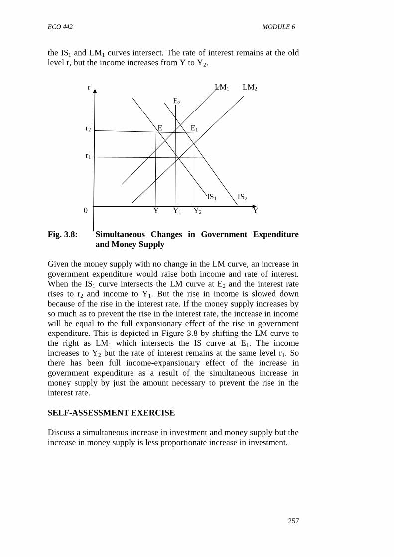
ECO 442 MODULE 6
257
the IS1 and LM1 curves intersect. The rate of interest remains at the old
level r, but the income increases from Y to Y2.
r LM1 LM2
E2
r2 E E1
r1
IS1 IS2
0 Y Y1 Y2 Y
Fig. 3.8: Simultaneous Changes in Government Expenditure
and Money Supply
Given the money supply with no change in the LM curve, an increase in
government expenditure would raise both income and rate of interest.
When the IS1 curve intersects the LM curve at E2 and the interest rate
rises to r2 and income to Y1. But the rise in income is slowed down
because of the rise in the interest rate. If the money supply increases by
so much as to prevent the rise in the interest rate, the increase in income
will be equal to the full expansionary effect of the rise in government
expenditure. This is depicted in Figure 3.8 by shifting the LM curve to
the right as LM1 which intersects the IS curve at E1. The income
increases to Y2 but the rate of interest remains at the same level r1. So
there has been full income-expansionary effect of the increase in
government expenditure as a result of the simultaneous increase in
money supply by just the amount necessary to prevent the rise in the
interest rate.
SELF-ASSESSMENT EXERCISE
Discuss a simultaneous increase in investment and money supply but the
increase in money supply is less proportionate increase in investment.

ECO 442 ADVANCED MACROECONOMICS
258
Mathematical Exposition of General Equilibrium of Product and
Money Market
Given the following models for XYZ economy:
C = 8 + 0.6Y where Y = income
I = 70 – 40r r = interest rate
Y = C + I C = consumption
L = 300 + 0.8Y - 160r I = investment
M = N400 L = demand for money
M = fixed money supply
Determine,
a. The IS function
b. The LM functions
c. The general equilibrium interest rate and income of the economy
Solution
(a) The IS function equilibrium of the IS occurs when:
Y = C + I
Y = 8 + 0.6Y + 70 – 40r
Y – 0.6Y = 78 – 40r
0.4Y = 78 – 40r
Y = 195 – 100r………………………………………….. (4.17)
(b) The LM function: Equilibrium of the LM occurs when:
L = M
300 + 0.8Y -160r = 400
0.8Y – 160r = 400 – 300
0.8Y = 100 + 160r
Y = 125 + 200r………………………………………….. (4.18)
(c) The general equilibrium requires simultaneous equilibria in both
markets thereby given the same values of Y and r, after solving
equations (4.17) and (4.18) simultaneously:
IS function: Y = 195 – 100r
LM function: Y = 125 + 200r
Equilibrium condition stipulates that,
IS = LM
195 – 100r = 125 + 200r
200r - 100r = 195 – 125
300r = 70
r = 70/300 = 0.23
Y = 195 - 100r alternatively, using equation (4.18):
Y = 195 – 100 (0.2333) Y = 125 +200r
Y = 195 – 23.33 Y = 125 + 200(0.2333)
Y = #171.7 Y = 125 + 46.66 = #171.7

ECO 442 MODULE 6
259
Graphically,
r LM
0.23 E0
IS
0 #171.7 Y
Fig. 3.9: General Equilibrium of XYZ Economy
SELF-ASSESSMENT EXERCISE
i. What is IS – LM framework?
ii. Algebraically and graphically illustrate the IS and LM curves
(functions).
4.0 CONCLUSION
The general equilibrium concept discussed in this unit involves finding
the equilibrium values of the interest and of output (income) in which
the product and money markets are in a simultaneous equilibrium. This
unit concludes the analysis we began in the previous unit where we
discussed equilibrium in product and money markets separately. The
working of fiscal and monetary policies in an economy was also
discussed. It is hoped that such knowledge can be applied to Nigerian
economy to achieve macroeconomics objectives.
5.0 SUMMARY
A discussion of the general equilibrium of products and money markets
has been undertaken in this unit. Equilibrium between S and I is possible
at all combinations of Y and r indicated by the IS curve; similarly,
equilibrium between L and M is possible at all combinations of Y and r
indicated by the LM curve. However, there is only one combination of
Y and r at which both I = S and L = M, and it is defined by the
intersection of the IS and LM functions. The general equilibrium
combination of Y and r identified by the intersection of the IS and LM
functions will, of course, change in response to any shift in those
functions. shifts in the IS function are caused by shifts in the investment

ECO 442 ADVANCED MACROECONOMICS
260
or saving function while shifts in the LM curve are caused by shifts in
the money supply or transactions demand or speculative demand
functions.
6.0 TUTOR-MARKED ASSIGNMENT
1. The following equations describe Nigerian economy
C = 0.9 (I – t) Y C = consumption
I = 300 – 600r I = investment
G = 600 G = government expenditure
t = 1/3 Y t = tax
L = 0.25Y – 150r L = demand for money
M = N375 M = supply of money
Y = income
r = interest rate
(i) Derive the IS function and its slope.
(ii) Derive the LM function and its slope.
(iii) What is the equilibrium level of income and interest rate in
this economy?
(a) Using the same equation:
(i) By how much will equilibrium income increases if
government increases its expenditure from #600 to #610?
(ii) By how much will interest rate decrease if money supply
increases from #375 to #385?
(iii) What is the new equilibrium level of income and interest
rate when these changes in (b) occur simultaneously?
Diagrams or graphs are necessary.
7.0 REFERENCES/FURTHER READING
Anyanwu, J.C. & Oaikhenan, H.E. (1995). Modern Macroeconomics:
Theory and Applications in Nigeria. Onitsha, Nigeria: Joanee
Educational Publishers Limited.
Branson, W.H. & Litvack, J.M. (1981). Macroeconomics. (2nd ed.).
Harper International Edition.
Jhinghan, M.L. (2003). Macro-Economic Theory (11th ed.). VRINDA
Publications (P) Limited.
Samuelson, P.A (1971). “The Simple Mathematics of Income
Determination: Income, Employment and Public Policy.” In:
Nueller, M.G. (Ed.). Readings on Micro Economics. New York:
Holt, Rinethart and Winston.
Shapiro, E. (1974). Macroeconomic Analysis. (3rd ed.). New York:
Harcourt Brace Jovanovich, Inc.

ECO 442 MODULE 6
261

ECO 442 ADVANCED MACROECONOMICS
262
MODULE 5 INFLATION AND UNEMPLOYMENT
Unit 1 Inflation
Unit 2 Unemployment
Unit 3 The Phillips Curve (Inflation – Unemployment Trade-off)
UNIT 1 INFLATION
CONTENTS
1.0 Introduction
2.0 Objectives
3.0 Main Content
3.1 Meaning of Inflation
3.2 Types of Inflation
3.3 Measurement of Inflation
3.4 Theories of Inflation
3.5 Causes of Inflation
3.6 Effects of Inflation
3.7 Measures to Control Inflation
4.0 Conclusion
5.0 Summary
6.0 Tutor-Marked Assignment
7.0 References/Further Reading
1.0 INTRODUCTION
Inflation is a highly controversial term which has undergone
modification since it was first defined by the neo-classical economists.
They meant by it a galloping rise in prices as a result of the excessive
increase in the quantity of money. They regarded inflation as “a
destroying diseases, born out of lack of monetary control whose results
undermined the rules of business, creating havoc in markets and
financial ruin of even the prudent” (Jhingan, 2003).
In this unit, attempt is made to define inflation from the point of view of
many scholars and schools of thoughts. We shall also study all theories
of inflation, types, measurement, causes, effects as well as policies to
fight inflation. But before we analyse them, it is instructive to know the
meaning of inflation.

ECO 442 MODULE 6
263
2.0 OBJECTIVES
At the end of this unit, you should be able to:
explain the meaning of inflation
enumerate and analyse the different types of unemployment
analyse the measurements, causes as well as the effects of
inflation with reference to Nigerian economy
mention policy measures to fight inflation.
3.0 MAIN CONTENT
3.1 Meaning of Inflation
One of the most difficult problems facing almost all the countries of the
world, a problem which appears to be defined as a high and persistent
rise in the price level is inflation. This implies that not every price
increase is termed inflation, a once for all rise in the price level may not
be termed an inflationary phenomenon. Again, prices of all goods and
services may not rise simultaneously or by the same proportion. Even if
the increase in price is over a prolonged period, it may not be considered
inflation if the rate of increase is considered minimal. Therefore, a
practical definition of inflation would be a persistent increase in the
general price level at a rate considered too high and therefore
unacceptable. There are other definitions of inflation but they are more
academic than practical. Examples are “the excess domestic demand
over domestic supply, the result of excess money creation” too much
money chasing too few goods etc.
The literature is full of a plethora of definitions of inflation. Solow
(1979) for instance, sees inflation as going on when one needs more and
more money to buy some representative bundle of goods and services,
or a sustained fall in the purchasing power of money. As Johnson (1972)
notes, and for most purposes, inflation is generally and conveniently
defined as a sustained rise trend in the general price level.
Economists often defined two different inflation – shock inflation and
core or steady state inflation quite apart from pure inflation.
a. Shock inflation
Shock inflation refers to a sudden change in the price level (including
wages) that is caused by a rise in the price of an important good or factor
of production. It is generally associated with supply shocks and
decreases in real income resulting from a change in the relative price of
factors compared to the price of goods. It occurs in one time spurts. For

ECO 442 ADVANCED MACROECONOMICS
264
example, large sudden fall in the relative value of a nation’s currency are
a typical cause of shock inflation.
b. Core or steady inflation
This is a steady, continual rise in the average price levels, not resulting
from a relative change in the price level over time. It is the underlying
rate of inflation when shock inflation has been adjusted out. The term
steady-state refers to the continual nature of the core inflation process.
In fact, the steady-state of a variable is the value at which the variable
eventually settles after it has been disturbed. Thus, if inflation rate has
settled at some particular value, then it is called the steady-state rate of
inflation.
c. Pure inflation
Economists focus on this theoretical concept in analysing inflation. A
pure inflation is that in which all prices, including wages and other
sources of income rise at an equal rate.
Today, however, economists refer to inflation as the continual upwards
movement of the general price levels.
SELF-ASSESSMENT EXERCISE
Based on the above definitions, construct in your own words, the
meaning of inflation.
3.2 Types of Inflation
a. Demand pull inflation
This type of inflation takes place when aggregate demand is rising while
the available supply of goods is becoming less. Goods may be in short
supply either because of resource is fully utilised or production cannot
be increased rapidly to meet the increasing demand. As a result, prices
begin to rise in response to a situation often described as “too much
money chasing too few goods”. This was the situation during the Biafra-
Nigeria war and after the Udoji Salary Awards of 1974 when wages
extensively increased. According to the demand pull theory, what
initiates a rise in the price level is the emergence of excess demands
over existing supply.

ECO 442 MODULE 6
265
P D1 D2 S
P2
P1
D2
0
D1 Q
Fig. 1.1: Demand Pull Inflation
While demand increased from D1D1 to D2D2, supply remained
unchanged, thus causing price to rise from P1 to P2.
b. Cost push inflation (Wage-Price-Spiral inflation)
This is indicated by rising cost of production, particularly rising wages.
If for instance, the cost of living of workers suddenly rises and they
demand and are granted higher wages, this increases cost of production.
This will be reflected in the form of higher prices on commodities which
consumers and workers have to purchase. This leads to workers to
demand for more wages since the initial increment has been eroded by
the rising prices. In fact, the cycle continues and prices continue to rise.
Hence, the name wage-price spiral.
Another cause of cost push inflation is profit push inflation.
Oligopolistic and monopolistic firms raise the price of their products to
offset the rise in labour and production costs so as to earn higher profits.
P S2 S1
P2
P1
S2 S1 D
0 Q
Fig. 1.2: Cost-Push Inflation

ECO 442 ADVANCED MACROECONOMICS
266
We observe from the above graph, that due to rising costs of production,
the supply has fallen from S1S1 to S2S2 thus leading to higher prices.
Here price increases from P1 to P2.
c. Hyper inflation
This type of inflation occurs when the price level rises at a very rapid
rate. In this case money loses its functions as a store of value and its
medium of exchange function may be affected if people are unwilling to
receive it, preferring trade by barter. This was the situation in Germany
after World War II in 1945 when people preferred cigarette to money.
The main cause of hyperinflation is an enormous expansion of the
money supply.
SELF-ASSESSMENT EXERCISE
Critically differentiate between demand pull and cost push inflation.
3.3 Measurement of Inflation
Basically, there are two widely used inflation measures in Nigeria, the
percentage change in the consumer price index and the Gross Domestic
Product (GDP) deflator.
a. The percentage change in the consumer price index as a
measure of inflation
Nigerian inflation can be seen as a percentage rate or change over a
specified unit of time (usually a year) in the consumer price index (CPI).
This is computed as follows:
Pt – Pt-1/ Pt-1 x 100……………………………..…………..(5.1)
Where Pt = Current period CPI
Pt-1 = Previous period CPI
b. GDP deflator
The GDP deflator is calculated by dividing the current price GDP by the
constant (base year) price GDP
GDP deflator = GDP in current prices /GDP at constant price……..(5.2)

ECO 442 MODULE 6
267
SELF-ASSESSMENT EXERCISE
Based on the difference between the percentage change in the consumer
price index and the GDP deflator, which one do you prefer and why?
3.4 Theories of Inflation
The literature identifies a number of theories of inflation, viz: demand
pull, cost push, structural monetary and imported inflation. However,
two competing theories of inflation are the Keynesian and the Classical
or Monetarist theories.
Keynesian theories of inflation: The debate between Keynesian and
monetarists with respect to inflation concerns the strength of competitive
forces. Thus, two separate Keynesian theories of inflation are
discernable: The quasi-competitive Keynesian theory of inflation and
the non-competitive Keynesian theory of inflation. However, for the
Keynesian, the arrow of causation in the equation of exchange MV = PY
is from right to left - increases in price cause increases in money, MV
← PY.
1. The quasi competing theory of inflation
The quasi-competitive Keynesian theory of inflation (as advocated by
James Tobin, Mancur Olson, James Meade, David Colander, etc.) states
that at competitive equilibrium “structural imperfections” inherent in a
monetary economy generate upward pressure on the price level. That is,
Keynesians see perfect competition as unstable in many markets,
because suppliers will seek rents by establishing institutions that will
prevent other potential suppliers entering the market. These activities,
called “invisible foot” place an upward pressure on the price level. As an
illustration, consider Figure 1.3 where the supply/demand equilibrium
price is Pe. Faced with such competitive equilibrium, individuals would
have strong incentives to “escape” the competition by joining with other
individuals (monopolise) to obtain a higher price for the goods they sell
and a lower price for the goods they buy. Thus, if suppliers of quantity
OA got together and prevented suppliers of quantity AB from entering
the market, their income would rise by the quantity represented by the
rectangle PeRHPm. They are therefore willing to spend up to that amount
to prevent competition from forcing price down. As they spend money
to create the necessary barriers to entry that will assure them in the
higher price, they create an upward pressure on the price in the market.

ECO 442 ADVANCED MACROECONOMICS
268
P D Suppliers who are kept out of market S
PM H
Rent for Group OA
PE R E
0 QM QE Q
Fig. 1.3: Forces of Monopolisation: The Quasi Competitive
Theory of Inflation
2. The non-competitive Keynesian theories of inflation
The non-competitive Keynesian theories of inflation generally assumes
the forces of competition to be so weak that a useful model of inflation
should not focus on competition or market forces; it should instead
focus on real world institutions or on specific institutional arrangements
in markets. Thus the first variant of these theories focuses on specific
markets - either the product market or the labour market and the
problem of inflation are discussed while centering on the institutional
arrangements in that particular market.
For early cost-push theories such as that by Gardner means focused on
the product-market monopolies and the monopolist’s profit as the cause
of inflation. However, the product-market emphasis was later dropped
while for later economists, it was fashionable to focus on the labour
market and wage-push inflation. These wage-push theories, which have
various forms, are the most popular in Keynesian literature. In some,
market forces are almost non-existent and wage levels are sociologically
determined. Peter Wile’s theory of inflation, for example, focuses on
wage inflation and it maintains that wage inflation is determined by the
whim of union leaders and is almost impervious to economic forces.
Thus, if union leaders decide to be unreasonable, money wages rise and
that increases is passed on via firm’s markup pricing procedures,
resulting in price inflation. The same reasoning and analysis was
followed by “Sidney Weintran’s earlier wage cost markup theory”. In
ECO 442 MODULE 6
269
this theory, it is postulated that once the nominal wage and price level
has risen, government has two options: it can either ratify the increase,
causing inflation, or it can refuse to ratify, causing unemployment. The
second variant of the non-competitive Keynesian theories of inflation is
called the leap-frogging models and they focus on normal wage
differentials or wage contours hence, the name wage contour theories.
Such views are advocated by John Hicks, Michael Piore, and others. To
them there are forces at work in the determination of money wages
which are noncompetitive. If wage differentials are disturbed for some
reasons, an inflationary process is set in motion, which again, can either
be ratified by the government or not ratified. The role of wages results in
a series of fixed relationship among the wage rates of certain groups of
jobs and workers, these relationships are known as wage contours. The
economy is composing of series of these more or less self-contained
contours, whose boundaries evolve overtime as the relationships within
them. When a wage breaks out of time, distorting one of the fixed
relationships, immense pressure is generated to restore it. Such pressures
emanate directly from rank-and-file workers and take the form of job
action and strikes. These consequently generate political and
organisational conflicts among various branches and division of such
bodies as trade unions and companies.
The view is that inflation is a two-part process. It is triggered by external
shocks, which drive wage within a stable contour out of line. Individuals
and institutions then react to restore the original differentials. The
process of restoration generates the bulk of the actual inflation. But the
initial factors are the strategic factors. Thus, leap-frogging theories
consider sociological and class variables much more important than
economic variables in determining relative wages.
Since wage contours adjust eventually, new “acceptable contours are
reached after a series of leap frogging wage increases. Therefore, the
wage contour theories are short run theories. What changes then to long
run theories of inflation is the assumption that the long run consists of
successive short runs, the theory provides for an ongoing inflation,
leaving the government with the dilemma of ratifying that inflation or
not. In all cases, accommodation of supply shocks results in higher
inflation but reduces unemployment rate. That is, policy makers
accommodate supply shocks when they increase the growth rate of
money to prevent unemployment that would otherwise occur as a result
of supply disturbance that shifts the short run Phillips curve.
(B) The monetarist theory of inflation
The earliest theory of inflation was based on the quantity theory of
money. According to the monetarist, inflation is always a monetary

ECO 442 ADVANCED MACROECONOMICS
270
phenomenon. They based their analysis using familiar Fisher’s equation
of exchange that is: MV = PQ.
According to this theory, if V and Q are held constants, the price level
(P) will vary proportionately with the supply of money (M). With
factors of production and technology changing slowly over time, while
the economy operates at full employment level, a doubling of the
quantity of money would simply double the price level. This would
leave individuals and firms with excess cash leading to a rise in prices.
According to M. Friedman, inflation is always and everywhere a
monetary phenomenon that arouses from a more rapid expansion in the
quantity of money than in total output”. He sees excess spending as a
result of rise in the nominal quantity of money supplied to the economy.
SELF-ASSESSMENT EXERCISE
Distinguish between Keynesian theories of inflation and monetarist
theory of inflation.
3.5 Causes of Inflation
In summary, many forces can cause inflation. On the demand side,
anything that shifts aggregate demand curve to the right will have this
result cater is paribus (increase in C, I, G, X–M, as well as relaxation of
monetary policy, or decrease in money demand). On the supply-side,
anything that increases cost of production leading to a shift of short run
aggregate supply to the left will cause the price level to rise.
In more explicit form, the under listed factors are the main causes of
inflation in Nigeria:
a. Excessive money supply over the available goods
The Udoji Salary Award of 1974 and the Minimum Wage Act of 1981
injected a lot of money into the economy which gave impetus to
inflationary trend in the economy.
b. Inadequate supply of goods and services
When the supply of goods and services fall short of the aggregate
demand, the tendency is raising prices. In Nigeria, the craze for
government employment without corresponding increase in productivity
has helped in fueling inflation.
ECO 442 MODULE 6
271
c. Deficit financing by government
Most developing countries through deficit budgeting can fuel inflation
when such expenditures are not directly tight to viable projects.
d. Rural-urban migration
A situation able-bodied men who are supposed to be producers of
agricultural products drifts to urban areas in search of other employment
and social amenities often causes inflation because of the decline in the
supply of agricultural products. This creates a serious demand gap that
force prices to rise.
e. Imported inflation
If a country depends for so much on imports from an inflationary
infested country, inflation in the exporting country will be readily
transmitted into the importing country.
f. Increase in population
Population growth in the developing countries is generally higher than
growth in productivity. For instance, Nigeria population that was about
55 million in 1963 rose to over 88.5 million in 1991 and by 2006; it has
risen to 140 million. This rapid growth in population without
corresponding growth in productivity puts aggregate demand in excess
of aggregate supply.
g. High cost of production
The high cost of production experienced by Nigerian industries is one of
the causes of inflation in Nigeria. Most of our raw material are imported
at high cost and coupled with the rising wage rate push production costs
higher which are transferred to the consumers in form of high prices.
h. Foreign exchange rate
The Nigerian economy, and of course most west African economies
depend heavily on the external sector for productivity of the domestic
economies leading to high exchange rates. This translated to high cost of
production resulting in inflationary pressures in these economies.
i. Indirect taxes
Are some of the cause of inflation in the country these taxes are shifted
to consumers in form of high prices of goods and services so affected.

ECO 442 ADVANCED MACROECONOMICS
272
j. The introduction of Structural Adjustment Programme
(SAP)
With its elements such as withdrawal of subsidies from agricultural
inputs and petroleum products, devaluation of currency, privatisation etc
have largely contributed to increase in inflationary tendencies in
Nigeria, especially in the late 1980s and 1990s
SELF-ASSESSMENT EXERCISE
Explain the various causes of inflation you know.
3.6 Effects of Inflation
Inflation affects people in different ways. When prices rise, certain
group of people benefit from the rise while some do not.
1. Inflationary trend causes disequilibrium in an economy while a
continuous substantial rise in the general price level is injurious
to the economy; a milder inflation acts as a stimulant to the
productivity of an economy. During this period, entrepreneurs
have high expectations of the future, investment is encouraged
which will bring about increase in demand for factor inputs. This
leads to a decline in the level of unemployment.
2. On redistribution of income and wealth, a high rate of inflation
brings about a redistribution of income in favour of businessmen
at the detriment of fixed income earners. In Nigeria, for instance
the SAP induced inflation brought harsh economic conditions on
the salary/wage earners and pensioners. The fixed income earners
suffer because their wages and salaries were not flexible while
prices of commodities continued to rise.
3. Inflation discourages savings. This is because the real value of
savings cannot be maintained. By discouraging savings, inflation
could be perpetuated because wealth owners would want to keep
their wealth in real assets as opposed to money.
4. During inflation period, debtors gain and creditors lose. During
this period, the value of money falls although debtors would
return the same amount of money borrowed during stability or
low prices, it will not be able to pay for the same units of
commodity it would at the time the loan was granted.
5. Loss of confidence in money. In extreme cases of hyperinflation,
money virtually becomes worthless. Supplier of factors of

ECO 442 MODULE 6
273
production would want to be paid in kind, and creditors will keep
away from debtors in order not to be paid worthless money.
Money will be deprived of its function as a medium of exchange
and as a store of value. It also ceases to function as a standard
unit of account because of the instability in the value of money.
SELF-ASSESSMENT EXERCISE
Assess the economic impact of inflation in Nigeria.
3.7 Measures to Control Inflation
Methods to control inflation are usually grouped under three headings;
monetary, fiscal and other measures
1. Monetary measures: These measures aim at reducing money
incomes. These include:
a. Credit control: The monetary authority adopts a number
of methods to control the quantity and quality of credit. It
raises the bank rates, sells securities in the open market,
raises the reserve ratio etc. This is effective when the
cause of the inflation is demand pull.
b. Demonetisation of Currency: The demonetisation of
higher denominations is usually adopted when there is
abundance of black money in the economy - the existence
of black money in all countries due to corruption, tax
evasion etc.
c. Issue of new currency: This involves the issues of new
currency in place of the old currency. Under this system,
one new note is exchanged for a number of notes of the
old currency.
2. Fiscal measures: Monetary measures alone cannot control
inflation but have to be supplemented by fiscal measures.
a. Reduction in unnecessary expenditures: The
government should reduce unnecessary expenditure, on
non-development activities in order to curb inflation.
b. Increase in taxes: To cut personal consumption
expenditure, the rates of taxes should be raised and even
new taxes should be levied, but the rate of taxes should not
be so high as to discourage saving, investment and
production.
ECO 442 ADVANCED MACROECONOMICS
274
c. Increase in saving: This will tend to reduce disposable
income with the people and hence personal consumption
with the people.
d. Surplus budget: Government should adopt an-anti
inflationary budgetary policy. It means collecting more
revenues and spending less.
3. Other measures
a. To increase production such as food, clothing etc.
b. Rational wage policy (freezing of wages, incomes,
dividends bonus etc.).
c. Rationing: This aims at distributing consumption of scarce
goods to essential consumer goods.
d. Price control: Fixing an upper limit for the prices of
essential goods.
SELF-ASSESSMENT EXERCISE
Enumerate and explain measures to control inflation.
4.0 CONCLUSION
This unit discussed inflation as a persistent and continuous rise in the
general price level. As one of the most difficult problem facing most
countries of the world, inflation is caused by so many factors like
excessive money supply over the available goods, inadequate supply of
goods and services among others. However, inflation can impact
positively in terms of productivity and negativity on fixed income
earners. Therefore, there is the need for government to put measures in
place to curb this ugly situation in an economy if people’s purchasing
power is to be maintained and not eroded.
5.0 SUMMARY
In this unit, the meaning of inflation has been explained as well as the
types and measurement of inflation. Theories of inflation have also been
discussed in details especially the Keynesian and the monetarist theories
of inflation. The unit equally discussed the causes, impacts of inflation.
As a result, measures put in place to control inflation were analysed. In
the next unit, we shall focus on unemployment.
6.0 TUTOR-MARKED ASSIGNMENT
1. Give a critical assessment of any theory of inflation and give
reason for selecting this particular theory.

ECO 442 MODULE 6
275
2. Distinguish between GDP deflator as a measure of inflation and
consumer price index as a measure of same. What are the merits
and demerits of each as a measure of inflation?
3. What strategies would you recommend in the fight against
inflation in Nigeria?
4. Distinguish between demand pull and cost push inflation; how
has these two views on inflation been reconciled?
7.0 REFERENCES/FURTHER READING
Anyanwu, J.C. & Oaikhenan, H.E. (1995). Modern Macroeconomics:
Theory and Applications in Nigeria. Onitsha-Nigeria: Joanee
Educational Publishers Limited.
Dutton, D. (1971). “A Model of Self Generating Inflation: The
Argentine Case.” Journal of Money, Credit and Banking. Vol.3,
No.2.
Ghatak, S. (1983). Monetary Economics in Developing Countries.
London: The English Language Book Society and Macmillan.
Jhinghan, M.L. (2003). Macro-Economic Theory (11th ed.). VRINDA
Publications (P) Limited.
Ochejele, J.J. (2007). Economic Analysis. Jos: Ichejum Publishers.
Shapiro, E. (1974). Macroeconomic Analysis. (3rd ed.). New York:
Harcourt Brace Jovanovich, Inc.

ECO 442 ADVANCED MACROECONOMICS
276
UNIT 2 UNEMPLOYMENT
CONTENTS
1.0 Introduction
2.0 Objectives
3.0 Main Content
3.1 Meaning of Unemployment
3.2 Types of Unemployment
3.3 Measurement of Unemployment
3.4 Causes of Unemployment
3.5 Effects of Unemployment
3.6 Measures to Fight Unemployment
4.0 Conclusion
5.0 Summary
6.0 Tutor-Marked Assignment
7.0 References/Further Reading
1.0 INTRODUCTION
Towards the end of the 19th century and the beginning of the 20th
century, one of the most troubling questions was the reason for
unemployment. Unemployment has been one of the most persistent and
imaginable problems facing all industrial countries of the world.
Unemployment has been defined as “involuntary idleness of a person
willing and able to work at a prevailing rate of pay but they do not find
work.” This definition implies that unemployment must be involuntary.
Voluntary unemployed persons who do not want to work like the idle
rich are not considered unemployed. Excluded also are those incapable
of work due to mental or physical disability. This unit introduces us into
another macroeconomic theory that has a lot of policy implications in an
economy. Hence, your attention is needed.
2.0 OBJECTIVES
At the end of this unit, you should be able to:
explain the meaning of unemployment
enumerate and analyse the different types of unemployment
analyse the measurements as well as the causes of unemployment
with reference to Nigerian economy
suggest policy measures to fight unemployment.

ECO 442 MODULE 6
277
3.0 MAIN CONTENT
3.1 Meaning of Unemployment
It is generally agreed that unemployment like inflation is a symptom of
basic economic illness or macroeconomic disequilibrium. What is
however controversial is the “appropriate” conceptualisation of the
subject. During the early days of the development of unemployment
theory, much controversy over the definition and origins of
unemployment revolved around the distinction between “voluntary” and
“involuntary” unemployment. Despite the difficulties of measurement
and norm-setting of the above classification, the taxonomy of
unemployment include a condition (being out of work), an activity
(searching for work), an attitude (desiring a job under certain
conditions), and a need (needing a Job (Levine, 1957).
The eight international conference of Labour Statistics held in 1954
gave rise to an International Labour Organisation (ILO) definition
concerning statistics of the labour force, employment and
unemployment. It sees the unemployment problem as having three
dimensions. The first dimension is determined by insufficient
employment possibilities involving disguised or open unemployment.
The second dimension is marked by an insufficient income structure.
Unemployment and poverty therefore constitute two different
viewpoints of one and the same problem. The third dimension is marked
by unproductive employment (underutilisation) of a considerable part of
the working population.
However in October, 1982, the 13th
International Conference of Labour
Statisticians adopted a new resolution concerning statistics of the
economically active population, employment, unemployment and
underemployment. The resolution defined the unemployed as persons
above a specific age who, during the reference period, were without
work, and were seeking work. This 1982 ILO definition, though similar
to the 1954 definition, includes certain amplifications and modification
for a more accurate measurement of unemployment.
SELF-ASSESSMENT EXERCISE
Give a working definition of unemployment in your own words.
3.2 Types of Unemployment
Basically, unemployment may be classified into two categories:
unemployment that results from deficient aggregate demand and all
other unemployment due to frictions and labour market (mal)

ECO 442 ADVANCED MACROECONOMICS
278
adjustments. The latter in turn is often divided into frictional, structural,
seasonal, real wage, technological cyclical unemployment.
a. Deficient demand unemployment occurs when there is not
enough aggregate demand to produce work for the whole labour
force, no matter how it is trained or deployed.
b. Frictional unemployment arises because it takes time and
resources for workers to change jobs, either voluntarily or
involuntarily, even though suitable job vacancies exist and can be
found without the worker having to adjust his broad occupational
status or his reservation wage.
c. Structural unemployment on the other hand, exists when there is
a mismatching between the unemployed and the available jobs in
terms of geographical location, required skills or any other
relevant dimension
d. Seasonal unemployment is seen as unemployment due to the
existing too high level of real wage. It normally results from
seasonal fluctuations in demand for example; agricultural
workers are employed during the peak of periods of sowing and
harvesting but remain idle for some periods of the year.
e. Technological unemployment arises when machines replace men
in the production process. This is a regular feature of
technological advanced nations of Europe and America.
f. Cyclical unemployment however, is traditionally associated with
the trade cycle, especially recession and depression. This explains
why some experts classify it as a variant of deficient demand
unemployment (Anyanwu, 1995).
SELF-ASSESSMENT EXERCISE
Compare and contrast between deficient demand and cyclical
unemployment.
3.3 Measurement of Unemployment
The unemployment rate (U) is measured as follows:
U = Number of unemployed/ Total labour force………. (5.3)
The labour force of any nation can be classified as “potential” and
“active”. The “potential labour force” refers to the entire population less
(a) young people below a prescribed age (usually 15 years), (b) old
people above a certain age (usually 65 years in most nations but 59 years
in Nigeria), (c) people who are institutionalised - those hospitalised/ in
penal or mental institutions /nursing homes, incarcerated, or physically
and mentally disabled, (d) full-time house wives, and (e) those unwilling
to work. Children (“age-ineligible population”) - those below 15 - are

ECO 442 MODULE 6
279
excluded on the assumption that schooling and child labour laws keep
most of them out of the labour force. These people excluded can be
regarded as “economically inactive population.”
However, the above measure of unemployment rate has been criticised
on the following grounds.
a. People who have part time temporary jobs are counted as
employed, even though they are significantly underemployed.
b. To be counted as unemployed, one must be looking for a job.
Many individuals have become so discouraged that they do not
even look and hence are not counted as unemployed.
c. Many individuals are working at unsatisfying jobs that do not use
their potential. They should be also counted as part of the
unemployment problem, at least underemployed.
SELF-ASSESSMENT EXERCISE
Analyse the measurement of unemployment and the criticisms therein.
3.4 Causes of Unemployment
a. Rising population. West African Population, particularly
Nigeria’s population is rising faster than job opportunities. A
situation in which birth rate is rising and death rate is falling.
b. Rural urban migration and neglect of agriculture. In Nigeria for
instance, since the oil boom days, there had been a neglect of the
agricultural sector and consequent mass exodus of able bodied
youths from the rural to the urban areas in search of non-existent
white collar jobs. This further reduces employment in agriculture
and puts pressure on existing urban jobs.
c. Tremendous expansion in educational opportunities and
investment in human capital. There has been a very rapid
expansion of primary, post primary and tertiary education in
West Africa which has given rise to an expanded labour market.
This has resulted to an influx of thousands of school leavers to
the cities in search of wage-employment.
d. Continuous shortfall in foreign exchange earnings and the
resultants fluctuation in the capital expenditure of governments.
Because most West African nations are mono cultural economies
(exporting of only one commodity) the fall in their prices such as
Nigeria’s oil) has led to decline foreign exchange earnings. This
has further led to decline in government’s capital expenditure
which would have been used to create jobs.
e. The problem of alien influx. As a result of the free movement
agreement of the Economic Community of West African states
(ECOWAS), there has been a rising influx of foreigners into the
relatively richer nations such as Nigeria. In addition, Asians are

ECO 442 ADVANCED MACROECONOMICS
280
in great number in West African countries. These aliens take up
jobs, sometimes at lower wage rates than could have been taken
up by nationals (Anyanwu, 1995)
f. Pre mature retirements and retrenchments. Most successive West
African governments on the protest of old age, ill health,
declining productivity, misconduct and other trivialities such as
inability to host the national flag engage in mass retrenchment
and premature retirements. The private sector also follows on the
ground of lack of raw materials and spare parts. This exercise in
Nigeria in 1975, 1984 and 1985 had gone a long way in
increasing the number of unemployed in the country.
g. Activities of Multinational Corporation. Most of the
multinationals in West Africa only engage in assembling and thus
employ only a handful of West Africans. In addition, they adopt
high technology methods of production (use of computers and
automated machines) thus causing technological unemployment.
h. Non-Revolutionisation of agriculture. The use of crude
implements such as hoes and cutlasses had made agriculture both
unattractive and unprofitable. This has gone a long way in
increasing the volume of unemployment in the sub-region.
SELF-ASSESSMENT EXERCISE
Discuss the causes of unemployment in developing countries.
3.5 Effects of Unemployment
a. Brain drain: Unemployment, especially among university
graduates, results in emigration of youths to other countries such
as advanced nations of Europe and America. This brain drain
leads to loss of highly educated and skilled manpower.
b. Increase in social vices and crimes: Frustrated unemployed
youths could be a recruiting source of armed robbery,
prostitution, economic saboteurs, drug trafficking, smuggling etc.
c. Increased rural-urban migration: Unemployment aggravates
rural-urban drift by youths who move to the cities in search of
non-existent jobs. This helps also to put pressure on existing food
and social amenities in the cities.
d. Fall in national output: Following Okun’s, law, a one per cent fall
in employment means a three per cent fall in output. Thus, the
existence of unemployment means that a nation cannot maximise
the use of its labour force increased output.
e. Increased drain on government finance: The presence of
unemployment means increased government expenditure for the
payment of unemployment benefits in nations where they are

ECO 442 MODULE 6
281
paid. The government also spends more for the provision of
social services at the same time that it collects less from taxes.
f. High dependency ratio: The mass of unemployment will have to
depend on the small number of the working population for their
survival. This will reduce efficiency and savings.
g. Fall in the standard of living: Unemployment through the
resulting poverty and income inequality reduces the standard of
living of the masses.
SELF-ASSESSMENT EXERCISE
Explain the causes of unemployment you know.
3.0 Measures to Fight Unemployment
a. Reduction of population rate: Government of West Africa should
adopt stiff measures to reduce population growth through family
planning, persuasion, coercion, financial incentives and
disincentives, legislation and education.
b. Tackling the alien influx: All illegal aliens in Nigeria and in the
West African sub region should be identified and deported
irrespective of their nationalities.
c. Fighting rural-urban migration: There should be integrated rural-
urban development programmes, re-orientation of economic
activity, social investments and the spread of small-scale labour
intensives industries in the rural areas to check rural-urban drift.
d. Modification or the direct linkage between education and
employment: Science, technology and skills appropriate and
necessary for our rural development should be emphasised in our
educational institutions. Skills inculcated in schools should be
relevant to industrial and commercial needs of the countries. The
successful implementation of the 6-3-3-4 system of education in
Nigeria will help make our graduates job creators rather than job
seekers.
e. Diversification of the base of the nation’s foreign exchange
earnings: Most West African countries should diversify their
mono-cultural economies so as to increase their revenues for the
creation of job opportunities.
f. Creation of national employment schemes: National employment
schemes, charged with the responsibility of collating reliable
information on the job matter should be created. It will undertake
the registration of the unemployed and make placements where
openings exist.

ECO 442 ADVANCED MACROECONOMICS
282
SELF-ASSESSMENT EXERCISE
Suggest other ways/measures of controlling unemployment in Nigeria.
4.0 CONCLUSION
Just like inflation, unemployment is seen as a symptom of basic
economic illness or macroeconomic disequilibrium in an economy. This
unit so far discussed unemployment as voluntary and involuntary
unemployment. Types and causes of unemployment have also been
discussed as well as the effects and measures to curb unemployment.
5.0 SUMMARY
This unit has analysed unemployment as a situation or condition being
out of work, an activity searching for work, an attitude desiring a job
under certain conditions, and a need, needing a job. The unit equally
discussed causes of unemployment and effects to include rural-urban
migration, brain drain, social vices and crimes among others. The unit
concludes with various measures to control unemployment. The next
unit discusses the Philip’s curve, an interaction of inflation and
unemployment.
6.0 TUTOR-MARKED ASSIGNMENT
1. Outline and discuss causes of unemployment in Nigeria. Identify
possible effects of the problem and suggest possible ways in
which it can be tackled.
2. Outline and explain four types of unemployment you know.
7.0 REFERENCES/FURTHER READING
Anyanwu, J.C. & Oaikhenan, H.E. (1995). Modern Macroeconomics:
Theory and Applications in Nigeria. Onitsha-Nigeria: Joanee
Educational Publishers Limited.
Levine, I. (1957). “Unemployment by Locality and Industry.” In: The
Measurement and Behaviour of Unemployment (MBER). New
Jersey: Princeton University, Press.
ECO 442 MODULE 6
283
UNIT 3 TRADE-OFF BETWEEN INFLATION AND
UNEMPLOYMENT (THE PHILLIPS CURVE)
CONTENTS
1.0 Introduction
2.0 Objectives
3.0 Main Content
3.1 Concept of the Philips Curve
3.2 Basic Tenets of the Philips Curve
3.3 Monetarist Challenge to the Philips Curve and the Long
Run Philips Curve (the Natural Rate Hypothesis)
4.0 Conclusion
5.0 Summary
6.0 Tutor-Marked Assignment
7.0 References/Further Reading
1.0 INTRODUCTION
Since wage cost represents the backbone of the price structure, in recent
years, the interest of economists in supply inflation has led them from
the examination of the relationship between the rate of price increase
and the rate of wage increase to an examination of the relationship
between the rate of wage increase and the rate of unemployment of the
labour force. If in addition to the direct relationship between the rate of
price increase and the rate of wage increase, there is also an inverse
relationship between the rate of wage increase and the rate of
unemployment, it follows that there is an inverse relationship between
the rate of inflation and unemployment rate. Because the data for
various countries and for various time periods do show this inverse
relationship between the rate of wage increase and the unemployment
rate, the unemployment rate in this indirect way becomes a factor of
major interest in the study of supply inflation.
2.0 OBJECTIVES
At the end of this unit, you should be able to:
explain the concept of the Philips curve
analyse the basic tenets of the Philips curve
discuss the monetarists’ challenge of the Philips curve and the
natural rate hypothesis.

ECO 442 ADVANCED MACROECONOMICS
284
3.0 MAIN CONTENT
3.1 Concept of the Philips Curve
The analysis of the particular relationship between the rate of wage
increase and the unemployment rate proceeds in terms of the “Philips
curve” so named after A.W. Philips who pioneered in the investigation
of this relationship for the United Kingdom. In its simplest form, a
Philips curve may be derived from an economy’s data for a period of
years by plotting for each year the percentage of money wage rate
increase, Δw/w (vertical axis), against the percentage of the labour force
that is unemployed, U (horizontal axis). A curve fitted to the points so
plotted will slope downward to the right like the hypothetical curve in
Figure 3.1. Any curve of this general shape suggests that the rate of
money wage increase is inversely related to the unemployment rate.
ΔW/W (%)
0 U
PC
Fig. 3.1: The Original Philips Curve
Philips had detected an inverse curve liner relationship between inflation
rate and the rate of unemployment in a statistical study of observed
annual figures for unemployment and money wage for the fifty two year
period 1861 – 1913. Other studies were for the period 1913 – 1948 and
1948 – 1957: Phillips approach was to draw a curve of best fit through
the scatter gram of observed combinations of unemployment and money
wage rate for the United Kingdom. The resulting curve exhibited a
negative shape, much like a demand curve.

ECO 442 MODULE 6
285
SELF-ASSESSMENT EXERCISE
Describe with the use of diagram the concept of the Philips curve.
3.2 Basic Tenets of The Philips Curve
A basic tenet of Philips curve is that a stable but inverse relationship
exists between unemployment and inflation rate as provided by money
wage rate changes. The continued existence of this observe stable
relationship was deemed to have far reaching implications for policy
makers, for it represented a menu of policy choice between inflation and
unemployment rate. This tenet of the Philip curve relationship meant
that policy makers could choose between inflation and unemployment in
the course of macroeconomic management. It meant that high levels of
employment (low unemployment could only be obtained by tolerating a
high rate of inflation. Conversely, a government desirous of achieving
low rates of inflation (stable prices) could do so only at the cost of high
unemployment rate. The existence of this tradeoff as revealed in the
Philips curve relationship explain the application of “the twin evil of
macroeconomics” with which both unemployment and inflation have
been dubbed.
Another tenet of the Philips curve is that, apart from the simultaneous
attainment of both objectives being in conflict, the attainable
combinations of both variables were known. Hence, the diagram shows
that a rate of inflation can be obtained only at a cost of an
unemployment rate of say 5.5 per cent. On the other hand, effort to
attain a 7.5 per cent rate of wage inflation would only be compatible
with a one per cent point rate of unemployment. In general, the relevant
policy trade-off, being the rates of exchange between policy goals at the
disposal of the authorities was reflected in the slope of the curve. Since
the existence of the tradeoff could be traced to the existence of inherent
conflicts among policy objectives, efforts to solve one of the policy
problems necessarily exacerbate the other. For example, the inability to
simultaneously achieve the goals of full employment and of price
stability means that efforts to move the economy closer to one of them
say, full employment will of necessity drift it farther and farther away
from the other, price stability. The rate of trade-off (the cost of attainting
a little lot more of one of the objectives as reflected in the magnitude of
the other that must be tolerated) is measured by the slope of the curve.
Thus, the steeper the curve the lower will be the decrease in
unemployment that will be brought about by large increase in the rate of
inflation.
On the other hand, the flatter the curve, the higher will be the fall in
unemployment that will be attained by a small increase in the rate of

ECO 442 ADVANCED MACROECONOMICS
286
inflation. The trade-off relationship implied by the Philips curve meant
that it was possible for policy makers to determine the opportunity cost
of a lowered inflation rate in terms of the employment forgone.
It was their task therefore to optimise this trade-off relationship by
selecting the inflation-unemployment-combination that maximised
social benefit or minimise social cost. Rational policy making of course
means that policy makers would settle for that combination that
minimise the social harm.
SELF-ASSESSMENT EXERCISE
Explain vividly the two basic tenets of the Philips curve.
3.3 Non-Trade-Off Philips Curve (The Natural Rate
Hypothesis)
Economists who speak in terms of “trade-offs” between a higher rate of
inflation and a lower unemployment rate or a lower rate of inflation and
a higher rate of unemployment view the Philips curve as a fairly stable
relationship along which policy makers may choose one position or
another. For example, if the objective is to move from an existing five
per cent unemployment rate to a three per cent rate, the goal can
presumably be achieved if we are willing to trade the higher rate of
inflation indicated by the Philips curve at the three per cent
unemployment rate for the lower rate of inflation that is found at the five
per cent unemployment figure. In other words, according to these
economists, if we are willing to pay the price in terms of inflation,
public policy is capable of moving an economy to a three per cent
unemployment rate or whatever other realistic rate is selected as a goal.
But there are many other economists who deny that society can in this
way trade-off more inflation for a lower unemployment rate on other
than a temporary basis. To them, the Philips curve of the conventional
type shown by curve PC in Figure 3.1 describes a short run or transitory
relationship that is valid only as long as discrepancies between expected
and actual price and wage changes prevail. According to these
economists, once such discrepancies have been removed, the Philips
curve of the conventional type ceases to exist. One of such economists
that challenged the existence of a stable relationship between inflation
and unemployment rate are the monetarists. The monetarists challenge
to the Philips curve was articulated in the presidential address of Milton
Freidman, President of the American Economic Association and High
priests of Monetarism in 1967, an address in which the Philips curve
was integrated into macroeconomic theory.

ECO 442 MODULE 6
287
The thrust of Friedman’s position was the absence of a long run tradeoff
between inflation and unemployment. Hence, he asserts that any
observed trade-off was at best a short run phenomenon. Friedman notes
that, there must be some level of unemployment that is consistent with a
cleared labour market (full employment situation). This level of
unemployment which he called the natural rate of unemployment is
characterised by an equilibrium real wage rate. This natural rate, also
known as non-accelerating inflation rate of unemployment (NAIRU)
was the result of imperfections in the labour market, resulting for
example, from imperfect flow of knowledge between job seekers and
job givers about job openings bringing about frictional unemployment.
Natural unemployment was also attributable to structural factors; bring
about unemployment of the structural variety.
Friedman noted that the NAIRU was an irreducible minimum which was
consistent with full employment. Consequently, the reduction of
unemployment below this rate via the tools of monetary and fiscal
policies he argued would at best be a temporary phenomenon, otherwise
an ever accelerating inflation would be the result should policy makers
attempt to make it a permanent phenomenon.
To illustrate Friedman’s view, assume an existing natural rate of
unemployment is five per cent or higher unemployment rate that is being
combated by expansionary monetary and fiscal policy. The expansion of
aggregate demand resulting from this policy will involve some upward
pressure on prices to P1 and some reduction in the real wage rate, thus
giving employers an incentive to expand output, and to do this they will
expand or reduce unemployment to U2. It therefore appears that a lower
unemployment rate may be obtained in exchange for some rise in prices.
However, workers will recognise before long that the higher prices have
reduce their real wage rate and will demand and secure higher money
wages to offset the rise in prices. This is illustrated on Figure 3.2 below.

ECO 442 ADVANCED MACROECONOMICS
288
C P2
E D P1 C B 0 U1 U2 U* U SRPC3 SRPC1 SRPC2
Fig. 3.2: Expectation-Argument Phillips Curve (The Natural
Rate Hypothesis)
Successful agitations increase their real wages but increase costs to
employers who respond by cutting back on employment. With an
increased price, remaining at P1 and a cut back in employment, the
economy will undergo an adjustment in the labour market characterised
by virulent stagflation, a period in which both inflation and
unemployment would co-exist in an intensified form. This situation
would persist until there is a return to the natural rate U*. Thus, the
transition to the natural rate is characterised by (1) a new Short Run
Phillips Curve (SRPC) labeled SRPC2 and (2) a new and higher rate of
inflation that is consistent with the natural rate labeled P2. The transition
path is denoted by the arrow labeled BC. The foregoing process will be
repeated if the government, again dissatisfied with the natural rate
attempts again to lower it beyond U* by implementing expansionary
fiscal and/or monetary policy. This could mean attempting to reduce U*
to U2 in the diagram. Again, expansionary fiscal monetary policies
trigger off increased prices, lowering the real wage rate if wage increase
lag behind price increases, enabling employers to hire more labour and
reducing unemployment, and achieving the goal of policy thereby, but at
a higher price level P2 than P1. However, wage increases are soon
negotiated and secured in response to the increased prices, raising the
real wage rate necessitating a cut back in employment by employers;
thus, increasing the unemployment rate until the natural rate, U*
restored. Again the return to this new rate is characterised by (1) the
movement to a new SRPC labeled SRPC3 and (2) a higher price level P2
with the transition path being defined by the arrow labeled DE, a path
characterised by another round of virulent stagflation. Eventually, point

ECO 442 MODULE 6
289
E is arrived at, the natural rate is restored but at a higher price level P2.
Eventually, a long run Philips curve labeled Long Run Phillips Curve
(LRPC) is traced out by the locus of the points formed by the successive
short run Philips curves such as C and E and the natural rate U*. This
LRPC, according to the monetarist is vertical in shape. Thus, we can
assert from the foregoing analysis that the monetarist challenge to the
Philips curve inflation – unemployment trade-off was deny its existence
at least in the long run, conceding that whatever is true of it is at best a
short run phenomenon. This position is partly summarised in Friedman’s
word that “there is always a temporary tradeoff between inflation and
unemployment, there is no permanent trade-off”.
SELF-ASSESSMENT EXERCISE
The monetarists assert that: “there is always a temporary tradeoff
between inflation and unemployment; there is no permanent trade-off.”
Discuss.
4.0 CONCLUSION
You have seen from the analysis that the basic concept of the Philips
curve is essential to the understanding of the twin evil of inflation and
unemployment in macroeconomic management. While Phillips claims
that there is a stable inverse relationship between inflation and
unemployment, the monetarist claims that such relationship only exist in
a short term whereas the long run Philips curve is vertical. A key policy
implication of the natural rate hypothesis is the dilemma faced by policy
makers in the course of trying to influence both variables.
5.0 SUMMARY
The unit has explained vividly the meaning of the Philips curve. The
basic tenets of the Philips curve are considered alongside the expectation
argument Philips curve - the natural rate hypothesis. The unit equally
looked at the non-trade-off Philips curve advocated by the monetarist
led by Milton Freidman, and finally graphical illustration of the long run
Philips curve were given to justify the long run Philips curve.
6.0 TUTOR-MARKED ASSIGNMENT
1. What were the major tenets of the Philips curve inflation-
unemployment tradeoff? How valid are they in real world
situation?
2. Discuss the Philips curve and bring out its apparent policy
implications.

ECO 442 ADVANCED MACROECONOMICS
290
3. What is NAIRU? What is the relevance of NAIRU in the non-
tradeoff Philips curves?
7.0 REFERENCES/FURTHER READING
Friedman, M. (1968). “The Role of Monetary Policy.” AER.
Philips, A.W. (1958). “The Relation between Unemployment and the
Rate of Change of Money Wage Rate in the UK 1861 –
1957.”Economics. Vol. 15.
Shapiro, E. (1974). Macroeconomics Analysis. (3rd ed.). New York:
Harcourt Brace Jovanovich Inc.

ECO 442 MODULE 6
291
MODULE 6 ECONOMIC GROWTH ANALYSIS AND
GROWTH THEORIES
Unit 1 Economic Growth Analysis
Unit 2 Economic Growth, Income Inequality and Environmental
Quality
Unit 3 Growth Theories/Models
UNIT 1 ECONOMIC GROWTH ANALYSIS
CONTENTS
1.0 Introduction
2.0 Objectives
3.0 Main Content
3.1 Meaning of Economic Growth
3.2 Distinction between Economic Growth and Economic
Development
3.3 Measurement of Economic Growth
3.4 Determinants of Economic Growth
4.0 Conclusion
5.0 Summary
6.0 Tutor-Marked Assignment
7.0 References/Further Reading
1.0 INTRODUCTION
By introducing such factors as consumption, investment and
governments expenditure and growth labour productivity into the static
model of simple economy to a complex one, we took the first steps away
from a purely static model of the economy towards a more dynamic
view. In this unit and of course this module, we move into a more
dynamic view of income and brief survey of dynamic models of
economic growth.
2.0 OBJECTIVES
At the end of this unit, you should be able to:
explain the concept of economic growth
analyse the distinction between economic growth and economic
development
discuss measurements of economic growth
state the sources of economic growth.

ECO 442 ADVANCED MACROECONOMICS
292
3.0 MAIN CONTENT
3.1 Meaning of Economic Growth
Economic growth for the underdeveloped countries is one of the four
macroeconomic goals of any society. Recall that others are price
stability, full employment and a healthy balance of payments position.
Modern economic growth refers to the development of the developed
counties of Western Europe, the United States, Canada, Australia and
Japan. Professor Simon Kuznets in his Nobel Memorial Lecture defined
economic growth “as a long-term rise in capacity to supply increasingly
diverse economic goods to its population, this growing capacity based
on advancing technology and the institutional and ideological
adjustments that it demands”. This definition has three components.
First, the economic growth of a nation is identified by the sustained
increase in the supply of goods. Second, advancing technology is the
permissive factor in economic growth which determines the growth of
capacity in supplying diverse goods to the population. Third for an
efficient and wide use of technology and its development, institutional
and ideological adjustments must be made to affect the proper use of
innovations generated by advancing stock of human knowledge
(Jhingan, 2003).
Anyanwu (1995) defined economic growth as to the increase over time
of an economy’s capacity to produce those goods and services needed to
improve the well-being of the citizen in increasing numbers and
diversity. It is a steady process by which the productive capacity of the
economy is increased overtime to bring about rising levels of national
income (Todaro, 1997). Thus, in discussing growth, it is imperative to
examine the behavior of the population overtime. This is because
economic growth becomes a meaningful concept if it leads to an
improvement in well-being of society overtime and this can happen only
if the rate of population growth lags behind that of economic growth
overtime. Thus, growth is a steady process of increasing the productive
capacity of the economy and hence of increasing national income, being
characterised by high rates of increase of per capita output and total
factor productivity, especially labour productivity.
Economic growth, according to Ochejele (2010) refers to the
quantitative and sustained increase in the country’s per capita output or
income accompanied by expansion in labour force, consumption, capital
and volume of trade.

ECO 442 MODULE 6
293
SELF-ASSESSMENT EXERCISE
From this scholarly definitions, produce a working definition of
economic growth.
3.2 Distinction between Economic Growth and Economic
Development
Growth and development are two inseparable worlds/concepts and often
used interchangeably to mean the same. Occasionally, this usage is
sometimes accepted. Where the two terms exist, separating their
meanings has merits.
Growth refers to increase, overtime, of an economy’s output of goods
and services. This definition does not take cognisance of desirable
structural changes in the society’s economic arrangement. Thus, while
growth refers to the volume of output in the current year vis-a-vis the
volume of output in a chosen previous years, it overlooks the
distribution to and hence the well-being of the citizens in the economy.
In contrast, the concept of economic development is more embracing for
it does not only concerns itself with issues of growth but also focuses on
the distribution of proceeds of growth. Thus, economic development is
generally defined to include improvements in material welfare
especially for persons with lowest incomes, the eradication of mass
poverty with its correlates of illiteracy, disease and early death, changes
in the composition of inputs and outputs that generally include shifts in
the underlying structure of production away from agricultural towards
industrial activities (Kindlerberger and Herrick, 1977).
It is a multidimensional process involving the provision of basic needs,
acceleration of economic growth, reduction of inequality and
unemployment, eradication of absolute poverty as well as changes in
attitudes, institutions and structures in the economy (Todaro, 1977).
Growth models are capable of expressing in a mathematical form but
development models cannot be easily expressed in a mathematical form
because of its complexity and the difficulty of some of the variables in
it. Therefore, the former can easily be subject to empirical measurement
and testing but it is sometimes more impossible to do same with the
latter.
Growth can occur without development, but it is impossible to perceive
development without economic growth. Therefore, there could be
growth without development if the increase in national income does not
have positive effects on the living conditions of the people, particularly
the poor.

ECO 442 ADVANCED MACROECONOMICS
294
SELF-ASSESSMENT EXERCISE
Growth and development are two inseparable concepts and often used
interchangeably to mean the same. Where the two terms exist,
separating their meanings has merits. Discuss.
3.3 Measurement of Economic Growth and Development
In discussing economic growth and development five strands of the
measure of growth can be deciphered. These measures include (1)
measurement of growth from the nominal perspective (2) growth
defined from real magnitudes (3) growth measured in terms of per capita
values (4) welfare, and (5) social indicators.
1. Nominal measurement of growth
Under the first measure of the concept economic growth is seen as the
increase in current value prices of aggregate products. This measure of
growth is based on an evaluation of the trend behaviour of aggregate
expenditure overtime. It is considered the crudest measure of the
concept as it does not take cognisance of such vital issues as to whether
or not the increased expenditure is matched by a concomitant increase in
the real value of output within the reference period.
2. Real output growth rate as a measure of economic growth
Determining whether or not the increased aggregate expenditure is
matched by an increase in real output overtime entails deflating the
nominal value of output by an appropriate price index to obtain the
corresponding magnitude. The deflated value of the nominal output
enables us to determine whether or not an economy has grown in real
terms overtime. Thus an economy is deemed to have grown in real terms
when there is an increasing aggregate output at constant price overtime.
3. GNP per capita
This measure relates to an increase in the per capita real income of the
economy. This indicator emphasised that for economic development to
occur, the rate of increase in the real per capita income should be higher
than the rate of growth of population.
Graphical representation of economic growth takes the form of an
outward shift in the economics’ PPF. Supposing the economy produces
two goods, say bread and butter with all its resources. Growth in this
hypothetical economy would be illustrated as shown below:

ECO 442 MODULE 6
295
Bread
PPC1 PPC2
0 Butter
Fig. 1.1: Economic Growth
The increase in economy’s output of bread and butters shown as the
outwards shift of the transformation curve from 1980 PPF labeled PPC1,
to that of 1990 labeled PPC2.
4. Welfare
Economic development can also be measured from the point of view of
welfare, in this case economic development is perceived to be an
increase in the consumption of goods and services.
5. Social indicators
Some economists that were dissatisfied with GNP and GNP per capita
have tried to measure economic development in terms of social
indictors. Hicks and Streeten (1979) as quoted by Ochejele (2010)
considers six social indicators for basic needs, which include health,
education, good, water supply, sanitation and housing. Social indicators
are often referred to as the basic needs to a higher level of productivity
and income through human development in the form of educated and
healthy people.
SELF-ASSESSMENT EXERCISE
Briefly explain the measurements of economic growth and development.
3.4 Determinants of Economic Growth
The determinants of economic growth can be broadly categorised into
economic and non-economic factors. Economic growth is dependent
upon economic factors such natural resources human resources, capital,

ECO 442 ADVANCED MACROECONOMICS
296
enterprises, technology etc. Non-economic factor such as social
institutions, political conditions and moral values also influence growth.
Economic factors
The growth rate of any economy depends on the changes of the factors
of production namely land, labour, capital and entrepreneurs.
Natural resources
One of the principal factors affecting development of an economy is the
natural resources otherwise known as land. Land as used in economics
includes natural resource such as the fertility of the land, its situation
and composition, forest resources, minerals, climate, water resources
etc. For economic growth to take place, the existence of these resources
is germane. In the LDCs, natural resources are unutilised, underutilised
or mis-utilised. The presence of abundant resources is only necessary
but not sufficient condition for economic growth. Growth requires
optimal exploitation and utilisation of these resources. As Fisher, J.L.
(1987) remarked “there is little reason to expect natural resource
development if people are indifferent to the products or services which
such resources can contribute”.
Some economists have argued that economic growth is possible even
when an economy is deficient in natural resources. Japan is one such
country which is deficient in resources but it is one of the advanced
countries today, because of its technology and how it has been able to
discover uses of its limited resources. Moreover, by importing raw
materials and minerals from other countries, it has been successful in
overcoming the deficiency of its resources through superior technology
researches. Thus, for economic growth to take place, the existence of
abundant natural resources and their proper exploitation coupled with
the relevant technology which will limit wastage for better utilisation.
Capital accumulation
Another important economic factor in growth is capital accumulation.
Capital represents the stock of physical reproducible factors which can
be acquired through the stock of physical money. The increase on the
capital stock over a period of time is capital accumulation. The process
of capital formation includes:
a. the existence of savings and the rise of them
b. the existence of credit and financial institutions to mobilise
savings and allocate them to the desired sectors; and
c. the use of these savings for investment.

ECO 442 MODULE 6
297
Capital formation is the main key to economic growth as it creates the
opportunity for future production. Capital formation helps in providing
machines, tools and equipment which are used in production process.
The provision of social and economic infrastructure like transportation,
education, health, power etc. is possible through capital formation. It
also leads to technology, exploitation of natural resources,
industrialisation and expansion of markets which are essential for
economic development.
In LDCs, the propensity to save is low hence, government often resorts
to forced savings by ways of taxation, deficit financing and borrowing.
Organisations
This is another factor that influences economic growth. It relates to the
optimum use of factors of production in economic activities. In modern
economics, the entrepreneur performs the role of an organiser. He is an
economic leader who possesses the capability and ability to recognise
opportunities for successful introduction of new commodities, new
techniques, and new sources of supply and to assemble the necessary
plant and equipment, management and labour force and organise them
into a running concern. Therefore entrepreneurship is indispensable in
economic development.
However, LDCs lack entrepreneurial capability. Such constraints as the
smallness of market, capital deficiency, technological backwardness,
lack of skilled and trained labour, non-availability of adequate raw
materials and infrastructure as well as increased risks and uncertainties
are major characteristics of the economies of the LDCs. The challenge
therefore is for the LDCs to create a climate that will encourage
entrepreneurship.
Technological progress
This is considered as one of the most important factor in the process of
economic growth. This relates to changes in the methods of production
which is the result of research and innovation. Technological changes
leads to increases in the productivity of labour and capital. Kuznets
traces five distinct patterns in the growth of technology in economic
growth. These are scientific discovery, invention, innovation
improvement and spread of invention. He therefore suggested that LDCs
must import technology to accelerate their productive capacity in the
short run because they cannot wait until they invent or modify the
technology of advanced countries.
Consequently, as they adopt the imported technology they must develop
their indigenous technical skills. This should be backed up by research

ECO 442 ADVANCED MACROECONOMICS
298
and development studies to enable them know the problems associated
with such technological adaptation. One of the principal factors of
economic growth has been huge spending on research and development
by the advanced countries.
Specialisation and division of labour
This also leads to increase in productivity. They lead to economies of
large-scale production which further help in industrial and agricultural
development. Division of labour leads to improvement in the productive
capacities of Labour, it saves time; it makes invention more feasible and
can widen the scope of market.
Structural changes
These are necessary ingredients for economic growth. Structural
changes imply the transition from the traditional agricultural dominated
economy to a modern industrial economy involving a radical
transformation of existing institutions, social attitude and motivations. It
implies reduction in the size of contribution to the net national output by
agricultural sector. This does not however imply a reduction of output in
absolute terms. It is its share in national income that has to decline
because secondary and tertiary sectors will now take the commanding
heights of the economy. Tertiary production includes a number of
dissimilar services like transport, retail and whole sale distribution,
education, government services etc.
Innovation or the opening of a new area may bring about a structural
change within an economy thereby widening the domestic and foreign
markets. Structural changes which affect technical skills, administrative
and entrepreneurial activities, transport and communication and supply
of capital are very important. To facilitate this process both money and
capital markets with their diverse instruments are required.
Non-economic factors
Non-economic factors play significant roles alongside with the
economic factors in the process of economic growth and development of
any country. Non-economic factors have much to do with human
endowment, social attitudes, political condition and historical accidents.
Therefore, social, cultural, psychological, political and administrative
factors are as much important as economic factors in economic
development. As pointed out by Cain cross in Jhingan (2003),
“development is not just a matter of having plenty of money nor is it
purely an economic phenomenon. It embraces all aspects of social
behaviour, the establishment of law and order, scrupulousness in
business dealings, including dealings with the revenue authorities,

ECO 442 MODULE 6
299
relationships with the family, literacy, and familiarity with mechanical
gadgets and so on.
In the area of social factors, issues regarding social attitudes, values and
institutions influence economic growth significantly. Attitude implies
the totality of beliefs and values that cause human behaviour to be what
it is. Western culture and education has led to reasoning and skepticism.
It inculcates the spirit of adventure which led to new discoveries and
inventions. People have cultivated the habit of savings and investments,
and undertaking risks so as to earn profits. They develop the will to
economise and to maximise output from a given input. As a result,
European countries experienced Industrial Revolution in the 18th and
19th centuries.
Human resources
Human resources have been an important factor in modern economic
development. Growth does not depend on the mere size of human
resources but on their efficiency. A proper use of human resources can
be made for economic development. To increase the productivity of
labour, emphasis should be placed on education and training. Thus as
Jhingan (2003) noted, “the most important requirement of rapid
industrial growth is people. People ready to welcome challenges of
economic change and opportunities in it. People, above all, who are
dedicate to the economic development of their country and to high
standards of honesty, competency knowledge and performance”.
Political and administrative factors
This also helps in modern economic development. The economic growth
of Britain, Germany the US, Japan and France can be explained in part
due to the political stability of these countries. Peace, protection and
stability have encouraged the development of entrepreneurship in
developed countries along with the adoption of appropriate fiscal and
monetary policies. The weak administrative and political structure is a
big hindrance to the economic development of LDCs. Thus the
government of LDCs must step up effort to offer services required for
economic development such as order, justice police and defense,
security, reward system etc. In this way, clean and strong administration
full of justice can stimulate economic development.
SELF-ASSESSMENT EXERCISE
Economic growth is determined by two types of factors. Enumerate and
explain these factors in relation to Nigerian economy.

ECO 442 ADVANCED MACROECONOMICS
300
4.0 CONCLUSION
The analysis above shows that economic growth is a more dynamic view
of economic progress. The distinction between growth and development
also helps in bringing out clearly the differences in ranking of countries
on the basis of growth and development. The measurement of economic
growth and development also helps in differentiating between growth
and development. The determinants of economic growth and
development tell us that such factors are complementary and not
substitute in the growth of an economy.
5.0 SUMMARY
The unit has thrown light on the meaning of economic growth. The
distinction between economic growth and economic development was
equally considered. The determinants of economic growth and
development were also looked at.
6.0 TUTOR-MARKED ASSIGNMENT
1. Economic growth and economic development are two concepts
used interchangeably to mean the same. Clearly distinguish
between these two concepts.
2. The process of economic growth is determined by two types of
factors. Succinctly explain these factors as it relates to Nigerian
economy.
3. Vividly explain the determinants of growth and development.
7.0 REFERENCES/FURTHER READING
Anyanwu, J.C.& Oaikhenan, H.E. (1995). Modern Macroeconomics:
Theory and Applications in Nigeria. Onitsha-Nigeria: Joanee
Educational Publishers Limited
Jhingan, M.L. (2004). The Economics of Development and Planning.
(37th revised ed.). Delhi, India: Nisha Enterprises.
Kindleberger, C.P. & Herrick, B. (1977). Economic Development.
McGraw Hill Book Company.
Ochejele, J.J. (2010). Macroeconomic Analysis. Jos: Ichejum Press.
Todaro, M.P. (1982). Economics for Developing World (2nd ed.).
Longman.

ECO 442 MODULE 6
301
UNIT 2 ECONOMIC GROWTH, INCOME
DISTRIBUTION AND ENVIRONMENTAL
QUALITY
CONTENTS
1.0 Introduction
2.0 Objectives
3.0 Main Content
3.1 Economic Growth and Income Distribution (The Kuznets
Hypothesis)
3.2 Economic Growth-Developed and Developing Economies
3.3 The Growth Rate and Environmental Quality
4.0 Conclusion
5.0 Summary
6.0 Tutor-Marked Assignment
7.0 References/Further Reading
1.0. INTRODUCTION
There has been much controversy among economists over the issue
whether economic growth increases or decreases income distribution.
Professor Kuznets is the first economist to study this problem
empirically. He observes that in the early stages of economic growth
relative income inequality increases, stabilises for a time and then
decline in the later stages. This is known as the invert U-shaped
hypothesis of income distribution.
2.0 OBJECTIVES
At end of this unit, you should be able to:
explain economic growth and inequality
discuss economic growth-developed and deeveloping economies
explain rate and environmental quality.
3.0 MAIN CONTENT
3.1 Economic Growth and Income Distribution (The
Kuznets Hypothesis)
In his 1955 study, Kuznets took the following data relating to three
LDCs (Less Developing Countries) - India, Ceylon (now Sri Lanka) and
Puerto-Rico, and two DCs (Developed Countries) - The UK and US.
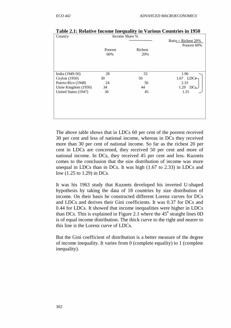
ECO 442 ADVANCED MACROECONOMICS
302
Table 2.1: Relative Income Inequality in Various Countries in 1950 Country Income Share %
Ratio = Richest 20%
Poorest 60%
Poorest Richest
60% 20%
India (1949-50) 28 55 1.96
Ceylon (1950) 30 50 1.67 LDCs
Puerto-Rico (1948) 24 56 2.33
Unite Kingdom (1950) 34 44 1.29 DCs
United States (1947) 36 45 1.25
The above table shows that in LDCs 60 per cent of the poorest received
30 per cent and less of national income, whereas in DCs they received
more than 30 per cent of national income. So far as the richest 20 per
cent in LDCs are concerned, they received 50 per cent and more of
national income. In DCs, they received 45 per cent and less. Kuznets
comes to the conclusion that the size distribution of income was more
unequal in LDCs than in DCs. It was high (1.67 to 2.33) in LDCs and
low (1.25 to 1.29) in DCs.
It was his 1963 study that Kuznets developed his inverted U-shaped
hypothesis by taking the data of 18 countries by size distribution of
income. On their basis he constructed different Lorenz curves for DCs
and LDCs and derives their Gini coefficients. It was 0.37 for DCs and
0.44 for LDCs. It showed that income inequalities were higher in LDCs
than DCs. This is explained in Figure 2.1 where the 450 straight lines 0D
is of equal income distribution. The thick curve to the right and nearer to
this line is the Lorenz curve of LDCs.
But the Gini coefficient of distribution is a better measure of the degree
of income inequality. It varies from 0 (complete equality) to 1 (complete
inequality).

ECO 442 MODULE 6
303
Fig. 2.1: The Lorenz Curve (LC) D
From Figure 2.1, the larger the coefficient, the greater the inequality.
The Gini coefficient is measured in Figure 2.1 as the ratio of area A/A +
B or A/Δ OCD. The greater is this ratio, the more unequal is the
distribution of income i.e., the more the Lorenz curve falls below the 450
line. In Figure 2.1, the area A covered by the rough Lorenz curve
roughly represents 37 per cent of the triangle OCD for DCs and the area
covered by the smooth Lorenz curve represents roughly 44 per cent of
the area of the triangle OCD for LDCs.
The changes in the distribution of income as measure by the Gini
coefficient in relation to the increase in per capita income trace out the
Kuznets inverted U-shaped curves K, as shown in Figure 2.2.
Gini 0.60
Coefficient 0.50
0.40
0.30
0.20 K
0.10
0
Per Capita Income
Fig. 2.2: The Kuznets Curve
Note that the more robust portion of the Kuznets curve lies to the right:
income inequality falls with an increase in per capita income at higher

ECO 442 ADVANCED MACROECONOMICS
304
levels of development. The variance around the estimated Kuznets curve
is greatest, however, from low to middle levels of development. The
inverted U-shaped curve hypothesis applies to the present developed and
developing countries but the degree of inequality in the latter is greater
than in the former.
SELF-ASSESSMENT EXERCISE
Explain in details the concept of economic growth and income
inequality as regard to Nigeria and the U.S.
3.2 Economic Growth-Developed and Developing Economies
The problem of growth is not limited to developed capitalistic
economies. In the area of pollution, the Volga Communist in Russia is
just as polluted as some of our major rivers in Nigeria, and pollution
runs in the streets in many developing countries. As there are
similarities, so there are differences. The sources of economic growth
are quite uniform for developed countries, and a quantitative study of
these sources for any developed country could precede along much the
same lines as those followed by Denison in his study of the U.S.
economy and eight western European economies. Although the relative
quantitative importance of each of the primary sources of growth will
not be the same in all developed economies, the primary sources
themselves will be the same. In the same way, a theory of economic
growth that attempts to explain the process by which growth takes place
in a developed economy will, in general, be applicable to any developed
economy. However, the same growth theory will not be applicable to a
developing economy. Since the next unit is devoted entirely to growth
theory relevant to developed economies, it may be helpful at this point
to mention the pertinent distinctions between growths in the two types
of economies.
To begin with, the most serviceable criterion for classifying economies
as developed or developing is per capita real income. Those with “low”
per capita income are considered to be developing; those with “high” per
capita real income are developed. Income is judged to be high or low by
comparing it to income in countries such as the United Kingdom and
Germany, which are relatively “high”. It is the level of absolute per
capita real income in the country relative to that in another that is
relevant for this classification. The parallel criterion for classifying
economies according to their growth rates for any particular period of
years is the rate at which per capita real income grows. Notice that
although developing countries are typically countries with low growth
rates, it is possible for such a country to show a high growth rate. If
ECO 442 MODULE 6
305
sustained, a high growth rate will clearly move the country out of the
“developing” class.
SELF-ASSESSMENT EXERCISE
Explain the most serviceable criterion for classifying economies as
developed or developing.
3.3 Economic Growth and Environmental Quality
From the late fifties through the mid-sixties, no economic issue received
more attention than the country’s growth rate. An annual growth rate for
a country indicates success in this direction. But at the same time that
this success was achieved, doubt began to arise as to whether this was
indeed a success in a more complete sense of that word. By the late
sixties there was serious questioning of a proposition that had long been
practically taken for granted – that the national well-being is enhanced
by an increase in the rate of output of the goods and services designed to
satisfy the needs of ultimate consumers currently and in the future. What
was by then being asked is whether there is a “tradeoff” between the rate
at which we expand the output of goods and services and the rate at
which the quality of the environment deteriorates. A more rapid rate of
growth means more of the goods and services that most people want, but
it also means more of the air, water, land, and noise pollution and
environmental damage that people do not want. With the awakening to
the seriousness of the pollution problem in the late sixties, economic
growth, which had long been generally viewed as something close to an
unmixed blessing, came to be viewed by the more extreme
environmentalists as something close to an unmixed evil.
It is, of course, true that pollution did not suddenly appear in the late
sixties. What did appear for the first time was the widespread awareness
of the fact that pollution had reached such proportions that, if allowed to
grow completely unchecked, it could destroy civilisation in the course of
not too many generations. Accompanying real GDP of #38923.2 in 1980
was a level of pollution that was apparently close to the assimilative
capacity of the natural environment and thus gave rise to no great
concern. However, twenty years later, in 2000, real GDP had increased
to #4582127 and with it probably came more than a proportional
increase in the amount of pollution and other poisons deposited annually
in the air and water and in the amount of environmental damage of
practically every other kind. It is easy to understand the opposition to
growth voiced by those who believe there is inevitably a close relation
between the rate of growth of GDP and the rate of decay of the
environment.
ECO 442 ADVANCED MACROECONOMICS
306
SELF-ASSESSMENT EXERCISE
Discuss the relationship between the growth of GDP and pollution.
4.0 CONCLUSION
It is observed in this unit that in the early stages of economic growth
relative income increases stabilises for a time and then decline in the
later stages. What is thus taken as given for the developed economies is
absent to a greater or lesser degree in developing economies. To move
up to the highroad of economic progress, developing economies must
typically undergo an economic and social reorganisation, and in some
cases even a transformation of the whole system, involving the adoption
of more advanced methods of production despite the cultural barriers to
such steps, the development of efficient transportation and
communications systems, the establishment of schools and facilities for
public services, and the development of modern monetary machinery
that includes a capital market and other credit facilities among others.
5.0 SUMMARY
This unit has explained economic growth and income distribution
popularly known as the Kuznets hypothesis. Kuznets comes to the
conclusion that the size distribution of income was more unequal in
LDCs than in DCs. The unit equally discussed growth rate and
environmental quality. A more rapid rate of growth means more of the
goods and services that most people want, but it also means more of the
air, water, land, and noise pollution and environmental damage that
people do not want.
6.0 TUTOR-MARKED ASSIGNMENT
1. How can economy increases it output as well as sustain the
environment in the long-run.
2. With aid of a diagram, explain vividly the Kuznets U-shaped
curve.
7.0 REFERENCES/FURTHER READING
Anand, S. & Kanbur, S.M.R. (1993). “The Kuznets Process and
Inequality-Development Relationship.” Journal of Development
Economics. February, 1993.
Jhingan, M.L. (2004). The Economics of Development and Planning.
(37th revised ed.). VRINDA Publications (P) Ltd. Delhi, India:
Nisha Enterprises.

ECO 442 MODULE 6
307
UNIT 3 THEORIES OF GROWTH AND
DEVELOPMENT
CONTENTS
1.0 Introduction
2.0 Objectives
3.0 Main Content
3.1 The Marxian Growth Theory
3.2 The Schumpeterian Growth Theory
3.0 The Classical Growth Theory
3.0 The Harrod-Domar Growth Model
3.0 The Neoclassical Growth Theory
4.0 Conclusion
5.0 Summary
6.0 Tutor-Marked Assignment
7.0 References/Further Reading
1.0 INTRODUCTION
There are several theories or models of various aspects of economic
growth and development process. These models have at all times being
the basis of policies aimed at helping the development processes along.
Our sole aim is to reveal these intellectual theories provided by different
scholars in the aspect of economic growth and development.
Although economic growth has been identified as one of the key
macroeconomic goals of society, issues of growth did not assume a
dimension of prominence until the mid-thirties. Two events largely
account for the outburst of interest in issues of growth. The first was the
publication of Keynes’ General Theory of Employment, Interest and
Money in 1936, who viewed deficiency in aggregate demand as the key
factor to economy’s stagnation. The second was the struggle to
overcome the devastating effect of the World War II on war ravaged
economies.
Interest in growth issues subsequently led to development of various
theories of growth each purporting to explain the mechanics of growth.
2.0 OBJECTIVES
At the end of this unit, you should be able to:
explain the Marxian growth theory
describe the Schumpeterian growth theory
discuss the classical growth theory

ECO 442 ADVANCED MACROECONOMICS
308
explain the Harrod-Domar growth model
discuss the neo-classical with respect to their limitations and
applicability to underdeveloped economies.
3.0 MAIN CONTENT
3.1 The Marxian Theory of Growth
One of the historical theories of economic growth, the Marxian theory of
growth is a mixture of reasoning proceeding from economics and
sociological perspectives. It proceeds by viewing growth as a process of
continue transformation of the society and social function and political
life. Such transformation can be traced to the society mode of
production as well as the property rights of the society, economic power
and prestige seeking class. Marxian growth theory asserts that growth is
dependent on the rate of accumulation of labour surplus value by the
capitalists’ class, labour surplus value being the rate of profit in excess
of labour’s true remuneration which has however, been expropriated
from the workers by their factors owners (the capitalists). Thus, the
Marxian theory of growth attributes growth to labour surplus value
which is the difference between subsistence wages paid to workers and
the true value of labour output. It is this difference that constitutes the
sources of investible fund necessary to foster economic growth.
Therefore, the larger this difference is, the more rapid growth is
expected to be. However, the Marxian theory of growth points at the
possibility of the eventual collapse of the capitalist systems resulting
from the intensification of the clash between the expropriators and the
expropriated.
SELF-ASSESSMENT EXERCISE
Explain vividly the Marxian theory of growth.
3.2 Schumpeterian Theory of Growth
Schumpeter appears to provide an answer to the problem raised by
Keynes theory through the very significant role he gives to the innovator
or the entrepreneur. Instead of the business minds expectation,
Schumpeter talks about the innovator who undertakes new combination
of factors of production. This combination opens the way for profits in a
statutory state or during a down turn which then leads to an upswing.
Also, instead of Keynes propensity to save, Schumpeter holds that, the
innovator/entrepreneurs secures the fund for his investment from the
banking sector - and the inflationary process which result from this,
forced people to save and higher capital accumulation is obtained.
Instead of the propensity to consume, he assumed that changes in taste
ECO 442 MODULE 6
309
are brought by the action of the entrepreneur, the lack of real resources
endangered by the inflationary process, the destructive competition that
followed the upswing or boom, the repayment of bank loan and the
effects which the cessation of innovative activity has on secondary
investment, all combined to bring about the down turn. Schumpeter
believes that the economic system is full of uncertainties and risks that is
inevitably discontinues or moves in a speed.
This theory has won great admiration from economists, but the
conclusions are not generally accepted. The criticism is that, there are no
longer innovators of the types assumed by Schumpeter - there are
instead large business units whose innovative activities and motivations
are not distinguishable from the ordinary business activities. Also view
from the developing countries point of view, Schumpeter type of
innovation is strictly the type from the developed world. Even if it exists
in a developing country, its effects will be limited because of
competition from the developed countries. This considerably lessens the
dynamism ascribed to innovation by Schumpeter. In addition, large
business units more easily absorb changes in economic environment and
plan for adjustment alone, therefore cannot explain the causes of down
turn.
It should be noted however, that, Schumpeter emphasis on innovator and
innovations is very important in the consideration of factors responsible
for economic growth. Equally important is his idea that sources of
investible funds is not just personal or corporate savings but the banking
system.
SELF-ASSESSMENT EXERCISE
i. Succinctly explain the Schumpeterian growth theory and the
limitations therein.
ii. Attempt a critique of the Schumpeterian growth theory and its
applicability to Nigerian economy.
3.3 The Classical Theory of Economic Growth and
Development
Without doubt the best known name in economics is Adam Smith. His
monumental work An Inquiry into the Nature and Causes of the Wealth
of Nations (1776) has had tremendous influences on scholars and
policymakers alike. As the title of the book indicates, Smith was mainly
concerned with the problem of economic development. He wanted to
discover how economic growth came about and what factors impede it.
It is interesting to know that no single compressive theory of growth and
development has emerged that has superseded the original work by

ECO 442 ADVANCED MACROECONOMICS
310
Smith. In his work, which most economists view as marking the
beginning of the classical economics, Smith sets forth the classical
principles of economic development. These principles are anchored on a
governmental policy of laissez-faire. The principle of division of labour
and the increase productivity brought on by the division of labour but
limited only by the extent of the market. As a result, free trade was
advocated as a way to promote this division of labour by exploiting each
nation’s comparative advantage in production.
Recent actions by less developed countries and policies advocated by
some developed economies are at odds with this laissez-faire principle.
Their argument is that government must direct the development process.
Many of these opinions grew out of the experience of the 1930s and the
1940s when Soviet Union was able to grow very rapidly by applying
severe authoritarian development techniques - as a result of this, the
Soviet Union development process was very successful given room for
economies from the underdeveloped world to attack the laissez-faire
principles. They began to argue that “no policy of economic
development can be carried out unless the government has the capacity
to adhere to it…” Quite often however, democratic government loses
touch and determination in the face of opposition. This is the dilemma of
most democratic government. It is here that Soviet countries have an
immense advantage; their totalitarian structure shields the government
from rigorous and reactionary judgment of the electorates.
The Classical theory can be summarised as follows:
Laissez-faire Policy: The classical economics believes in the
existence of an automatic free market which is an economy free
from government interference. It is the invisible hand doctrine
commonly associated with Adam Smith which maximises the
material income.
Capital accumulation. Capital accumulation was accepted as the
key to economic progress. All classicists regarded capital
accumulation as the only way to economic prosperity and by
extension to political leaderships. They therefore, lay emphasis
on large saving.
Profits as an incentive to investment. Profits induce investment,
the larger the profit the larger the capital accumulation and
investment.
Criticism of the classical theory of growth
The simple and abstract classical theory of development is not free from
criticism.
ECO 442 MODULE 6
311
i. Neglect of the public sector. To the classicists, the perfect
competition and the institution of the private sector were
essentially prerequisite for economic development. They have
however, failed to realise the important of the public sector in
accelerating capital accumulation, and so preached by the
classical.
ii. They ignore the middle class. The whole classical analysis was
based on socio economic environment prevailing in Britain and
certain part of Europe. It assumed the existence of a rapid
division of society between the capitalists and the proletariat or
labourers. It neglected the whole of middle class which provides
the necessary impetus to economic growth. It did not occur to the
classical that the major source of saving in an advanced society
was the income receive and not the property owners.
iii. Unrealistic growth process. The classical theory assumed a
stationary stage in which there was no change, but hovered
around a point of equilibrium, even where there were
disturbances, such was transition and temporary and can be
restored through the automatic device.
SELF-ASSESSMENT EXERCISE
Review the justification of the public sector in the economic affairs of a
nation.
3.4 The Harrod-Domar Growth Model
The model is a product of two scholars: Professor Roy Harrod of Britain
(1939) and Evsey Dommar of USA (1946). It is actually a growth
theory and it emphasises one of the components of the big-push - capital
which has always been considered important for economic development.
The source of capital is mainly saving consequently, in order to achieve
economic development; saving or capital formulation must increase over
a period of time. This of course should result in relative decrease in
consumption which in turn is necessary if rapid economic growth is to
be achieved. A key objective of the Harrod-Domar Model is to
overcome the limitation inherent in the short-run nature of the simple
Keynesian model. This model takes cognisance of only one of the dual
roles of investment in the economy, its role as a component of aggregate
demand. However, the dual role of investment as (1) a component of
aggregate demand and (2) as an addition to the stock of productive
resources must be accommodated in any long-run analysis for it to be
meaningful. This is because net investment has both a demand and
supply effect.
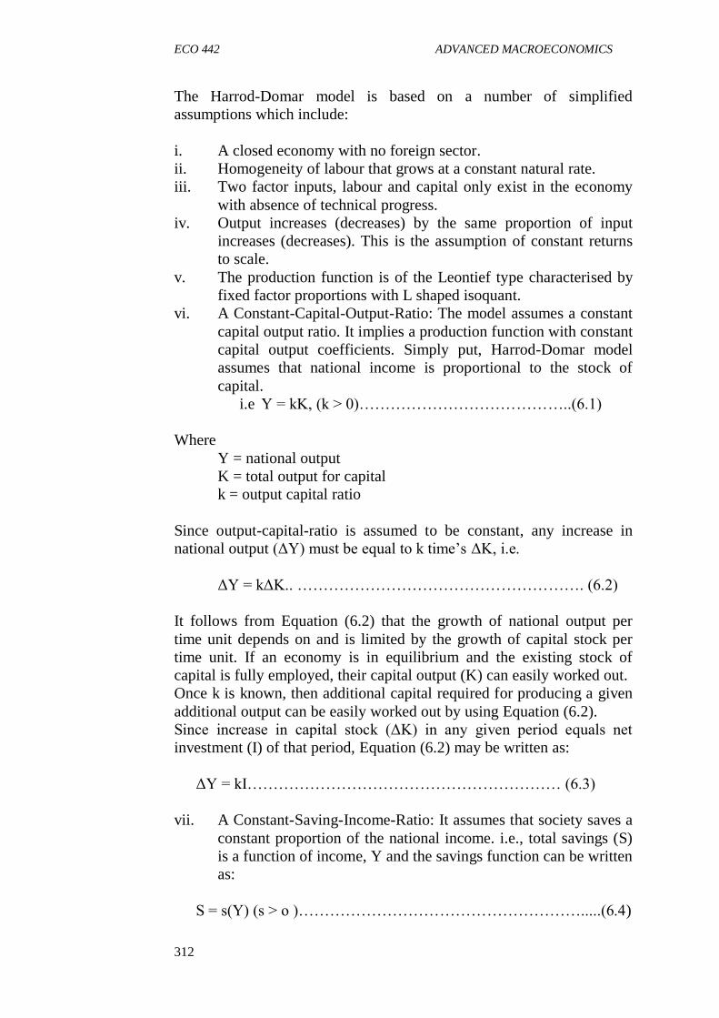
ECO 442 ADVANCED MACROECONOMICS
312
The Harrod-Domar model is based on a number of simplified
assumptions which include:
i. A closed economy with no foreign sector.
ii. Homogeneity of labour that grows at a constant natural rate.
iii. Two factor inputs, labour and capital only exist in the economy
with absence of technical progress.
iv. Output increases (decreases) by the same proportion of input
increases (decreases). This is the assumption of constant returns
to scale.
v. The production function is of the Leontief type characterised by
fixed factor proportions with L shaped isoquant.
vi. A Constant-Capital-Output-Ratio: The model assumes a constant
capital output ratio. It implies a production function with constant
capital output coefficients. Simply put, Harrod-Domar model
assumes that national income is proportional to the stock of
capital.
i.e Y = kK, (k > 0)…………………………………..(6.1)
Where
Y = national output
K = total output for capital
k = output capital ratio
Since output-capital-ratio is assumed to be constant, any increase in
national output (ΔY) must be equal to k time’s ΔK, i.e.
ΔY = kΔK.. ………………………………………………. (6.2)
It follows from Equation (6.2) that the growth of national output per
time unit depends on and is limited by the growth of capital stock per
time unit. If an economy is in equilibrium and the existing stock of
capital is fully employed, their capital output (K) can easily worked out.
Once k is known, then additional capital required for producing a given
additional output can be easily worked out by using Equation (6.2).
Since increase in capital stock (ΔK) in any given period equals net
investment (I) of that period, Equation (6.2) may be written as:
ΔY = kI…………………………………………………… (6.3)
vii. A Constant-Saving-Income-Ratio: It assumes that society saves a
constant proportion of the national income. i.e., total savings (S)
is a function of income, Y and the savings function can be written
as:
S = s(Y) (s > o )……………………………………………….....(6.4)

ECO 442 MODULE 6
313
Where S = savings
s = constant propensity to save.
At equilibrium level of output, the desired savings must be equal to the
desired investment i.e.
S = I = sY…………………………………………… (6.5)
Given the assumptions, the growth rate defined as ΔY/Y may be
obtained as follows:
ΔY/Y =Yt – Yt-1)/Yt
Where:
Yt-1 = national output in period t – 1
Yt = national output in period t
It may be infer from Equation (6.3) that in period t,
ΔYt = kIt…………………………………………………… (6.6)
By substitution, Equation (6.6) may be written as:
Yt - Yt-1 = k. s Yt…………………………………………. (6.7)
Equation (6.5) tells us that the Harrod-Domar model assumes that at
equilibrium in period t,
It = St = Yt
By substituting sYt for It in Equation (6.7) we get:
Yt - Yt-1 = k. s Yt……………………………………….(6.8)
By dividing Equation (6.8) by Yt, we get the growth rate ΔY/Y or what
Harrod calls the warranted growth rate Gw as:
Gw = Yt – Yt-1/Yt = ΔY/Y = k.s……………………… (6.9)
Where Gw is the warranted growth rate
Equation (6.9) shows that the rate of growth equals the output-capital-
ratio times the constant propensity to save. Since growth rate pertains to
the condition that I = S, this may also be called equilibrium growth rate
which implies capacity utilisation of capital. This growth rate fulfilled
the expectations of the entrepreneur. Therefore, this growth rate has
been termed as warranted growth rate.
Harrod-Domar defines Gw as that rate of growth which if it occurs, will
leave all parties satisfied that they have produced neither more nor less
than the right amount.

ECO 442 ADVANCED MACROECONOMICS
314
According to the Harrod-Domar model, a target growth rate can be
attained either by increasing the marginal propensity to save and
increasing simultaneously the stock of capital or by increasing the
output-capital-ratio.
Capital accumulation and labour employment under Harrod
Domar model
We have so far discussed the Harrod-Domar model of growth with
respect to only one aspect of the model i.e. capital accumulation and
growth. We now discuss another important aspect of the model i.e.
employment of labour. In the Harrod-Domar model, labour can be
introduced to the model under the following assumptions:
1. that labour and capital are perfect complement instead of being
substitute for one another
2. that capital-labour ratio is constant.
Under these assumptions, given the capital-labour-output-ratio,
economic growth can take place only so long as the potential labour
force is not fully employed. This implies that a potential labour supply
imposes a limit to economic growth at the full employment level. This
means:
(i). That growth rate will take place beyond the full employment only
if supply of labour increases.
(ii). That actual growth rate will be equal to a warranted growth rate
(Gw) only if growth of labour force equals the warranted growth
rate (Gw). If labour force increases at a lower rate, the only way
to maintain the growth rate is to introduce the labour-saving
technology. Under this condition the long-term growth rate will
depend on:
a. growth rate of labour force ( ΔL/L)
b. the rate of progress in labour-saving technology.
Thus the maximum growth rate that can be sustain in the long run will
be equal to ΔL/L plus a factor n i.e. the rate at which capital substitute
labour.
Harrods calls this growth, the natural growth rate (GN).
GN = ΔL/L + n……………………………………….. (6.10)
Limitations of the Harrod Domar Model
1. Unrealistic assumptions: The Harrod-Domar propositions that
savings will always increase to match with investment need is

ECO 442 MODULE 6
315
based on the assumption that the warranted growth rate is equal
to the actual growth rate. This is possible only under the
following simplified assumptions of the model:
MPC remains constant
output capital ratio ( k) is constant
the technology of production is given
the economy is initially in equilibrium
there is no government expenditure and no foreign trade
there are no lags in adjustment between:
a. demand and supply
b. savings and investment.
Since these assumptions make the modern economy unrealistic,
the warranted or expected growth rate may not always be equal to
the actual or realised growth rate. And if warranted and actual
growth rate are not equal there will be economic instability.
2. Another major defect of the model is that the parameters
used namely: Capital output ratio, marginal propensity to save,
growth rate of labour force, progress rate of labour saving
technology are all determined independently out of the model.
The model therefore, does not ensure the equilibrium growth rate
in the long run. Even the slightest change in the parameters will
make the economy deviate from the path of equilibrium.
In spite of these limitations, the Harrod-Domar model had been
used in development planning of many countries. Besides, it has
a great analytical power.
One key policy implications of the Harrod-Domar model is that the
growth rate of the economy can be influenced by policy makers by
tinkering with components of the warranted growth rate. This means that
by designing policies to influence the saving rate or enacting policies to
reduce the output-capital-ratio say, by investment in human capital,
productivity of capital can be increased hence the growth rate of the
economy can be considered a policy variable.
SELF-ASSESSMENT EXERCISE
i. Explain the warranted rate of growth as contained in the Harrod-
Domar model.
ii. Discuss the assumptions of the Harrod-Domar model and the
limitations therein.

ECO 442 ADVANCED MACROECONOMICS
316
3.5 The Neoclassical Growth Model
In one sense, neoclassical growth theory stands at an opposite extreme
from Harrod-Domar. In place of the Harrod-Domar assumption of a
single production process that imposes a fixed ratio between capital and
labour is the assumption of an indefinitely large number of production
processes, one shading off from another in a way that permits any
combination of labour and capital to be employed. Capital is thus
regarded as a unique, abstract agent of production that can be adjusted at
any time to absorb into employment a labour force of any size. With the
combination of labour and capital capable of varying in this way, it
follows that, instead of the fixed ratio between output and capital
employed by Harrod-Domar, the output capital ratio is also capable of
varying continuously. Thus, the larger the labour force absorbed into
employment with a given stock of capital, the greater will be the output
capital ratio, or the productivity of capital and the smaller will be the
output-labour ratio or the productivity of capital and the higher the
productivity of labour. These results follow simply as a matter of
diminishing returns.
In order to explain the model, it begins by pointing out the differences
and similarities between the assumptions of the Harrod-Domar and
Classical growth models.
1. While the production function implicitly in the Harrod-Domar
model contains only one factor i.e. capital, the neoclassical
growth model assumes a multifactor production function
including capital, labour and technology.
2. In the Harrod Domar, labour and capital are deemed to be perfect
complement of one another where as in the Neoclassical model,
capital and labour are assumed to be substitute for one another.
3. While Harrod-Domar model assumes a constant capital output
ratio, the neoclassical model assumes a variable capital output
coefficient. Incidentally, both models assume that capital and
labour are subject to the law of diminishing marginal returns to
scale.
4. In addition, the neoclassical model assumes perfect competition
where factor prices equal their marginal revenue productivity.
According to the neo classical model, rate of economic growth
depends on growth rate of:
- Capital, K;
- Labour supply, and
- Technological progress over time, T.
The relationship between the national output and these variables maybe
expressed in the form of a production function i.e.:

ECO 442 MODULE 6
317
Y = f (K, L, T)…………………………………….. (6.11)
Where:
Y= national output
L = Labour supply
K = stock of capital
T = the scale of technological progress
If technology assumes to remain constant for the sake of simplicity, then
the growth rate depends on K and L. The production function then takes
the following form:
Y = f ( K, L )……………………………………..….. (6.12)
Given the assumption of constant returns to scale, if the increase in L is
not very great in the period in question, the increase in Y will be
approximately equal to the increase in L times the marginal physical
product of L, or ΔY = MPPL. ΔL in which MPPL is the marginal
physical product of labour or the increase in Y that accompanies a unit
increase in L with K held constant. If we had assumed an increase in K
with no change in L, under the same assumptions, we would have had
ΔY = MPPK.ΔK in which MPPK is the marginal physical product of
capital or the increase in K with L held constant. Finally, for changes in
both K and L in a given time period we may write:
ΔY = MPPK.ΔK + MPPL.ΔL……………………….…. (6.13)
Dividing both sides by Y, we have:
ΔY/Y = (MPPK)/Y.ΔK + (MPPL)/Y.ΔL
This may also be written as:
ΔY/Y = (MPPK/Y.K)ΔK/K + (MPPL/Y.L) ΔL/L………. (6.14)
If we recall the assumption noted earlier of perfect competition markets
and now adopt the marginal productivity theory of factor pricing, each
unit of a factor will be paid its marginal product, and the total earnings
of capital and labour will equal to MPPK.K and MPPL.L respectively.
Given that factors are paid their marginal products, the total earnings of
capital and labour will exactly absorb the total output in the case of the
present production functions with constant returns to scale that is:
MPPK.K + MPPL.L = Y…………………………….. (6.15)
Since:
MPPK.K/Y + MPPL.L/Y = Y/Y = 1…………………………. (6.16),

ECO 442 ADVANCED MACROECONOMICS
318
We may substitute b for the first term on the left and (1 – b) for the
second term and rewrite equation (6.14) in the following form:
ΔY/Y = b (ΔK/K) + (1-b) (ΔL/L)……………………… (6.17)
The magnitude of b indicates the proportion of the total product or of
total income that would be received as a return on capital if capital were
paid its marginal product. This is the same as saying that b measures the
elasticity of output with respect to changes in the amount of capital used.
The same kind of statement may of course be made for labour by
making the appropriate substitutions in the second preceding sentence.
Assuming a value for b = 0.25, we may read from equation (6.17) the
percentage change in output that will follow from a given percentage
change in capital, labor or both. If both K and L rise by 3 per cent,
output also rises by 3 per cent, for the underlying production function is
one with constant returns to scale. In this case, we have:
ΔY/Y = 0.25 X 3 + 0.75 X 3 = 3
Like the Harrod-Domar model, the neoclassical growth model implies
that the path and speed of an economy’s growth are endogenous policy
variables that are within the ambit of policy makers.
SELF-ASSESSMENT EXERCISE
Attempt the derivation of the neoclassical growth model and the policy
implications therein.
4.0 CONCLUSION
This unit analysed the theories of economic growth using different
models. The conditions necessary for economic growth in each model
were explained. It is seen that despite their limitations the models have
great analytical powers in explaining the conditions for economic
growth, particularly the Harrod Domar and the neoclassical growth
theories.
5.0 SUMMARY
This unit provided us with the theories of economic growth. The basic
conditions necessary for economic growth were discussed. We
differentiated between Marxian and classical theories as well as the
Harrod Domar and the neoclassical growth models. The unit ended it
analyses on the mathematical derivation of the models under Harrod-
Domar and Neoclassical as well as some policy implications for
economic growth.
ECO 442 MODULE 6
319
6.0 TUTOR-MARKED ASSIGNMENT
1. What is warranted rate of growth? What were the major
limitations in the Harrod-Domar growth model which the
neoclassical model seeks to rectify? Hence explain the thrust of
the neoclassical growth model.
2. Comment briefly on the policy implications of the Harrod-Domar
and Neoclassical growth models.
3. Attempt a critique of the Schumpeterian growth theory. How
applicable is the theory to Nigerian economy.
7.0 REFERENCES/FURTHER READING
Anyanwu, J.C. & Oaikhenan, H.E. (1995). Modern Macroeconomics:
Theory and Applications in Nigeria. Onitsha-Nigeria: Joanee
Educational Publishers Limited.
Domar, E. (1946). “Capital Expansions, Rate of Growth and
Employment.” Econometrica, Vol. 14.
Harrod, R.F. (1948). Towards a Dynamic Economics. Macmillan.
Todaro, M.P. (1982). Economics for Developing World (2nd ed.).
Longman.