NATIONAL OPEN UNIVERSITY OF NIGERIA … · 2017-03-09 · PHY 192 INTRODUCTORY PRACTICAL PHYSICS II...

$: NATIONAL OPEN UNIVERSITY OF NIGERIA … · 2017-03-09 · PHY 192 INTRODUCTORY PRACTICAL PHYSICS II 2 In this experiment, you will practically experience refraction through the glass$
NATIONAL OPEN UNIVERSITY OF NIGERIA

COURSECODE:PHY192

COURSE TITLE: INTRODUCTORY PRACTICAL PHYSICS II

COURSE GUIDE PHY 192

ii

PHY 192 INTRODUCTORY PRACTICAL PHYSICS II Course Writer Dr. Sanjay Gupta Associate Professor School of Science and Technology National Open University of Nigeria Lagos And Prof. C. O. Ajayi

Physics Department, Ahmadu Bello University Zaria

Programme Leader Dr. Sanjay Gupta Associate Professor School of Science and Technology National Open University of Nigeria Lagos

NATIONAL OPEN UNIVERSITY OF NIGERIA

COURSE GUIDE


iii

National Open University of Nigeria Headquarters 14/16 Ahmadu Bello Way Victoria Island Lagos Abuja Office No. 5 Dar es Salaam Street Off Aminu Kano Crescent Wuse II, Abuja Nigeria e-mail: [email protected] URL: www.nou.edu.ng National Open University of Nigeria 2007 First Printed 2007

ISBN: 978-058-939-2 All Rights Reserved Printed by …………….. For National Open University of Nigeria


iv

CONTENTS PAGE Introduction……………………………………………. 1 Course Objectives……………………………………... 1 – 2 Getting Set for the Practical…………………………… 2 – 3 Report of Experiment…………………………………. 3 Summary………………………………………………. 4

Introduction This physics practical course PHY 192: INTRODUCTORY PRACTICAL PHYSICS II is an integral part of your physics course, which reinforces some, if not all, the principles, theories and concepts you must have learnt in the courses PHY 190: Basic Apparatus in Physics and PHY 142: Geometric and Wave Optics. Moreover, the physics practical is to enable you to know about the common apparatus like Cells, Potentiometer, Mirrors, Lens, and Resistors etc. Also, mirrors, lenses and/or prisms are the basic components of almost all image forming optical instruments. That is why there are some experiments on optics in this physics lab involving these devices. This physics practical course is divided into two modules. Module I is pertaining to Optics practical and Module II has experiments on Electricity. Each module contains 5 experiments. In all, there are 10 experiments. You must have read about optical apparatus and electrical components in your physics course PHY 190: Basic Apparatus in Physics. The experiments of this practical course PHY 192 are based on PHY 190 physics course. The experiments are as follows: Module I Experiments In Optics 1. Refraction through the glass block 2. Image formed by concave mirror 3. Determination of the focal length of the convex lens 4. Refraction through a triangular prism 5. Determination of the focal length of a converging lens and the

refractive index of the groundnut. Module II Experiments In Electricity 1. Determination of resistance of resistors in series and in parallel in

simple circuits. 2. Determination of internal resistance of a dry cell using a

potentiometer 3. To compare EMFs of two cells using a potentiometer 4. To determine the unknown resistance of a resistor using

Wheatstone Bridge. 5. Determine the relationship between current through tungsten and

a potential applied across it. Course Objectives The objectives of this Physics Laboratory Course are to:

PHY 192 INTRODUCTORY PRACTICAL PHYSICS II

ii

Develop some manipulative skills in handling some physics apparatus; and

Learn the process of scientific enquiry i.e. taking observations, analyzing and deriving conclusions.

The contents of the experiments are presented in the simplest forms. In the beginning of each experiment, a brief theory of each experiment is discussed to make you clear about the experiments with the help of labeled diagrams. Procedure of each experiment has been presented in the simplest form. You have to carry out the experiment step-by-step as mentioned in the procedure. You are expected to go through all the experiments before coming to laboratory work. For successful completion of an experiment, you should master skills of making measurements on a given apparatus, analyze data, and quote results. To quote the results with correct number of significant figures, you have already learned about ‘Measurement’ and ‘Error Analysis’ in PHY 191: Introductory Practical Physics I. It is very important to mention here that, in particular, you should be very clear about the concept of graph paper and its use to express the result in a physics experiment. Here, you will use this technique of graph paper to obtain the results of the experiments. In this course, you will perform 10 experiments as mentioned earlier. Before performing the experiment, you should familiarize yourself with the apparatus. If you like to have a deeper understanding into some aspects, you can refer other books on physics practical. It is to advise you that before going to the laboratory, you must posses the following: 1. A mathematical set containing the protractor, set squares, pair of

compass, short ruler and pencils. 2. A soft rubber (eraser) 3. 18cm long transparent plastic ruler 4. A scientific notebook with graph sheets to record your

experiments 5. Four-figure table and or a scientific calculator 6. French curves for drawing graphs. Getting Set for the Practical You are expected to read the write-up of the experiment, as many

times as possible, before coming to laboratory.


iii

You should have a clear idea about the experiment and the apparatus.

On the day of the experiment, you make sure that you assemble

all the apparatus required from the laboratory technologist. Set up the apparatus carefully and neatly on the working bench. Determine before hand how you will establish the physical

quantities to be measure. Examine the apparatus very well before the commencement of

the experiment to ensure that they are working very well. If not, make necessary correction (You may take the help of your facilitators).

Once the apparatus is set, record your observation in your

notebook in a tabular form and draw inferences. If required, draw the graph and calculate the slope and draw

result using the graph. Report of Experiment The report of each experiment should start from a fresh page in your notebook. The following must be clearly written in the following order: 1. Date when the experiment was performed 2. The aim and objectives of the experiment 3. Formula used 4. The circuit diagram (usually for experiments on electricity) 5. Table of observations 6. Graph 7. Calculation of slope or the constant 8. Estimation of errors where possible 9. Result. There is no need to write in your report, the section on apparatus, procedure, and theoretical consideration. All these are already contained in your test book. Only formula used is to be written. You are required to spend not more than 3 hours in performing and reporting the experiment each time you are in the laboratory. At the end of this period, you are required to submit your experiment for assessment.


iv

Summary The course, PHY 192: Introductory Physics Practical II enables students to develop some manipulative skills in handling physics apparatus like mirrors, lens and prism or to develop skills in making electrical circuits by using resistances, potentiometer, Wheatstone bridge etc. It is divided into two modules. Module I deals with the optical experiments in which mirrors, lens, prism etc. are used. On the other hand, in Module II, handling of apparatuses like potentiometer, Wheatstone bridge, determination of equivalent resistances and prism are discussed. In all, 10 experiments are discussed to familiarize students about the basic apparatuses in physics (in particular about optics and electricity). We wish you success!


v

Course Code PHY 192 Course Title Introductory practical Physics II Course Writer Dr. Sanjay Gupta Associate Professor School of Science and Technology National Open University of Nigeria Lagos And Prof. C.O. Ajayi

Physics Department, Ahmadu Bello University

Programme Leader Dr. Sanjay Gupta Associate Professor School of Science and Technology National Open University of Nigeria Lagos NATIONAL OPEN UNIVERSITY OF NIGERIA


vi

National Open University of Nigeria Headquarters 14/16 Ahmadu Bello Way Victoria Island Lagos Abuja Office No. 5 Dar es Salaam Street Off Aminu Kano Crescent Wuse II, Abuja Nigeria e-mail: [email protected] URL: www.nou.edu.ng

National Open University of Nigeria 2007

First Printed 2007

ISBN: 978-058-939-2

All Rights Reserved Printed by ................. For National Open University of Nigeria


vii

TABLE OF CONTENTS PAGE Module 1 Experiments in Optics….………………… 1 Unit 1 Refraction Through the Glass Block………. 1-5 Unit 2 Image Formed by Concave Mirror…………. 6-9 Unit 3 Determination of the Focal Length of the Convex Lens………………………… 10-15 Unit 4 Refraction Through a Triangular Prism……. 16-21 Unit 5 Determination of the Refractive Index of the Material of a Plano-convex Lens Using a Spherometer .……………. 22-26 Module 2 Experiments In Electricity………………… 27 Unit 1 Determination of Resistance of Resistors in Series and in Parallel in Simple Circuit……. 27-31 Unit 2 Determination of Internal Resistance of a Dry Cell Using a Potentiometer……………… 32-37 Unit 3 To Compare EMFs of Two Cells Using a Potentiometer………………………………… 38-42 Unit 4 Determine the Unknown Resistance of a Resistor Using Wheatstone-Bridge…………… 43-49 Unit 5 Determine the Relationship Between Current Through a Tungsten and a Potential Applied Across it………………………………………. 50-53


1

MODULE 1 EXPERIMENTS IN OPTICS Unit 1 Refraction Through the Glass Block Unit 2 Image Formed by Concave Mirror Unit 3 Determination of the Focal Length of the Convex Lens Unit 4 Refraction Through a Triangular Prism Unit 5 Determination of the Refractive Index of the Material of a

Plano-convex Lens Using a Spherometer. UNIT 1 REFRACTION THROUGH THE GLASS BLOCK CONTENTS 1.0 Introduction 2.0 Aims and Objectives 3.0 Main Content

3.1 Apparatus 3.2 Procedure 3.3 Data Processing

4.0 Result 5.0 Conclusion 6.0 Precaution 1.0 INTRODUCTION In our PHY 124 Geometric and Wave Optics course, you have studied about refraction in Unit 3. You will recall that when a light ray travels through a transparent surface (i.e. glass surface), the ray is bent at the surface. This bending of a ray of light is called refraction as shown in Fig. 1.1. This refraction obeys the laws of refraction.

Normal

C

Glass

Refracted ray

Incident ray

Fig. 1.1


2

In this experiment, you will practically experience refraction through the glass block. To do this, you will trace a ray of light that is incident on one side of the glass block which after passing through the glass block gets on the other side of the glass block. You will then be able to determine from the ray trace, the angle of refraction at each of the parallel (long plane) surfaces of the glass block. So after obtaining the angle of refraction, you will verify the laws of refraction and also determine the refractive index,, of the glass block using Snell’s Law:

= ri

sinsin where i is the angle of incidence and r is the angle of

refraction. 2.0 AIMS AND OBJECTIVES AIMS The aims of this experiment are to enable you to: practically verify the laws of refraction using a glass block; and determine the refractive index of a glass (glass block). OBJECTIVES After successfully completing all aspects of the experiment, you will be able to: trace a ray incident on one surface of the glass through the glass

to the other surface of the glass block; identify the incident and refracted ray; identify an angle of incident and an angle of refraction at a plane

surface; verify practically the laws of refraction; verify Snell’s law; and determine refractive index of the glass. 3.0 MAIN CONTENT 3.1 Apparatus Rectangular glass block, Drawing board, Optical pins, Thumb tacks, and


3

Sheet of paper. 3.2 Procedure 1.0 Fix the white sheet of paper on the drawing board with a thumb

tack at each edge of the paper. 2.0 Place the glass block on the paper and trace out its boundary

with a pencil. Then label the trace out rectangular as A, B, C, & D with the parallel longer side been AB and DC respectively as shown in Fig. 1.2.

3.0 On side AB mark a point Q such that AQ is approximately a half of QB.

4.0 Then draw the normal NQ to side AB at that point. Then with your protractor, measure an angle PQN equals 10 and draw line PQ. This line PQ is an incident ray and angle PQN is an angle of incidence (i).

5.0 Now insert two erect pins at point P and Q respectively. The pins inserted on these points should be straight and view the two pins from side DC of the glass block.

6.0 As you view these two pins, insert another set of two erect pins at points R and S such that the four pins fall on the same straight line.

7.0 This occurs when the four pins move together in one direction (as you move your head or your eye from one side of line RS to the other) that is, when there is no parallax (relative motion) between the four pins. You must ensure that the pins should be in a line before removing the glass block.

8.0 Remove the glass block and draw line RS and also line RM normal to side DC at R.

9.0 Measure angle SRM. 10.0 Draw line QR and RM′.

C

B

Glass slab

M

e R

r

M'

S

A

D

N'

Q r

P

i

N

Fig. 1.2


4

11.0 Then measure angles N′QR and angle M′ RQ. 12.0 Repeat the experiment using either sheet of white paper, three

times for angle NQP equals 20, 30 and 40 respectively. 13.0 Record all your observations in a Table 1.1 given below. In case

you have any difficulty, you may consult to your facilitator. 3.3. Data Processing In your first tracing paper, identify the followings: The incident ray and the refracted ray at Q and R, and The angle of incident and the angle of refraction. TABLE Complete the Table given below by calculating sin i and sin r for refraction at point Q and R respectively.

Table 1.1

Reading Angle NQP (i)

Sin i Angle NQR (r )

Sin r =

rsinisin

Angle QRM

(i)

Sin i Angle SRM (r)

Sin r =

rsinisin

1st 2nd 3rd 4th Now you should plot a graph between sin i and the corresponding sin r. Conventionally we plot the independent variable along the x-axis and the dependent variable along y-axis. Which quantity will you plot for this experiment along x-axis? Draw the best fit through observed points. Determine the slope for points Q and R respectively. To calculate the slope, you should use two widely separated points. 4.0 RESULT The refractive index of the glass of a slab is= ……... 5.0 CONCLUSION (i) What conclusion can you draw concerning with the laws of

refraction in this experiment. (ii) What are the slopes of sin i versus sin r graph for refractions at Q

and R respectively.


5

(iii) What can you deduce about the slope of sin i for refraction at Q and why is it different from that sin r at P?

(iv) What relationship exists between the slope for the curve of P and why is it so?

(v) What conclusion can you draw from this concerning Snell’s law? 6.0 PRECAUTIONS

The position of the glass slab should not be disturbed. All the four pins should be in the straight line. The two pins erected should be straight. The slope should be taken carefully.


6

UNIT 2 IMAGE FORMED BY CONCAVE MIRROR CONTENTS 1.0 Introduction 2.0 Aims and Objectives 3.0 Main Content

3.1 Apparatus 3.2 Procedure 3.3 Data Analysis

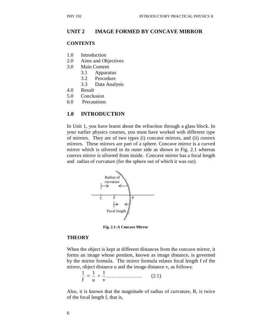
4.0 Result 5.0 Conclusion 6.0 Precautions 1.0 INTRODUCTION In Unit 1, you have learnt about the refraction through a glass block. In your earlier physics courses, you must have worked with different type of mirrors. They are of two types (i) concave mirrors, and (ii) convex mirrors. These mirrors are part of a sphere. Concave mirror is a curved mirror which is silvered in its outer side as shown in Fig. 2.1 whereas convex mirror is silvered from inside. Concave mirror has a focal length and radius of curvature (for the sphere out of which it was cut). THEORY When the object is kept at different distances from the concave mirror, it forms an image whose position, known as image distance, is governed by the mirror formula. The mirror formula relates focal length f of the mirror, object distance u and the image distance v, as follows:

f1 =

u1 +

v1 ………………… (2.1)

Also, it is known that the magnitude of radius of curvature, R, is twice of the focal length f, that is,

P

Focal length

C F

Radius of curvature

.

Fig. 2.1: A Concave Mirror

.


7

R = 2f……………………….. (2.2) If the object is kept in front of a concave mirror between its focus (F) and centre of curvature (C), the image formed is real, inverted and bigger than the size of the object (enlarged). Using the Eq.(2.1) and Eq.(2.2), focal length and radius of curvature can be obtained easily. So in this experiment, for a given concave mirror of unknown focal length, the image distances for a given set of known object distances use to locate it. A set of data will then be analyze graphically to determine the unknown focal length of the mirror. Eq. 2.1 suggests that if u and f are known, v can be determined. In fact, the Eq. 2.1 suggests that if two of the parameters are known then the third parameter can be determined. 2.0 AIMS AND OBJECTIVES This experiment is meant to enable you to practically carry out and apply the mirror formula to determine the focal length and hence the radius of curvature of a concave mirror as such. After successfully carrying out the experiment, you should be able to: determine the approximate focal length of a concave mirror; remove parallax between image and image pin; measure object distance and image distance;

plot a graph of u1 versus

v1 ; and

deduce the true focal length of a concave mirror. 3.0 MAIN CONTENT 3.1 Apparatus Concave mirror with holder, an optical bench, and two mounted pins. 3.2 Procedure 1. Obtain a rough value for the focal length of a concave mirror by

focusing the image of a distant window on to a sheet of paper


8

2. .The distance between the sharpest image on the paper or on the wall gives the approximate focal length of the mirror. Measure the distance and record in your note book as fo.

3. Now, place one of the pins (called the object pin, O) between F and C of the concave mirror as shown in Fig. (2.2). Here, F is the principal focus and C is the centre of curvature of the mirror. Note its position from the pole of the mirror which is u.

4. Similarly place the image pin. Now move the image pin beyond

C. Locate the position of the image by means of this pin (called the image pin, I) using the method of no parallax., which will also be near to C but on the opposite side (along CQ). You should be careful that the tips of the pins should be at the same height.

5. Note that this second pin also produces an image coincident with the object pin.

6. Measure the distance (u) of the object pin and the distance (v) of

the image pin from the pole P of the mirror.

7. Move the object to four different positions between F and C and also consequently the image pin to four positions along CQ (see Fig. 2.1) and note the readings of u and v each time.

R

O F .

Fig. 2.2

. .

Object needle u

v

C I Q . P

Image needle

(Pole)

Concave Mirror


9

3.3 Data Analysis Complete the Table 2.1 given below and compute the values of

u1 and

v1 . Tabulate your results as below:

TABLE Table 2.1 Reading u(cm) v(cm)

)cm(u1 1 )cm(

v1 1

vuf111

1 2 3 4 5 For each set of values of u and v, calculate corresponding values

of u1 and

v1 . Obtain the values of focal length by using Eq. (2.1).

Once the value of f is known then calculate the value of R. 4.0 RESULT The focal length of a concave mirror is = ………cm The radius of curvature of the concave mirror is= ……….cm 5.0 CONCLUSION (i) Deduce the focal length of the mirror. (ii) Deduce the radius of curvature of the mirror. (iii) What is the accuracy of fo compare to its true value? (iv) What conclusion can you draw from this experiment? 6.0 PRECAUTIONS The parallex should be removed from tip to tip. The tips of the centre of the concave mirror used and the needle

should be at the same height. The image formed should not be distorted. The graphs should be drawn very carefully choosing the

appropriate axis.


10

UNIT 3 DETERMINATION OF THE FOCAL LENGTH OF A CONVEX LENS

CONTENTS 1.0 Introduction 2.0 Aims and Objectives 3.0 Main Content

3.1 Converging Lens 3.2 Apparatus 3.3 Procedure 3.4 Data Analysis

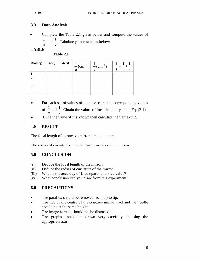
4.0 Result 5.0 Conclusion 6.0 Precaution 1.0 INTRODUCTION In your school you must have learnt in your optics course in physics that there is a relationship between the object and image distance measured from the pole of the lens. But the question that immediately comes to our mind is: what happens to the position of image if we change the position of object? If the position of object changes, one can locate the position of image accordingly. So, once you know the object and image distance, then one can determine the focal length of the given lens graphically as well as by applying the lens formula. Many methods can be used to determine the focal length of a convex lens. In this Unit, you will use a simple method known as u-v method to determine the focal length of a convex lens. In the earlier Unit, you have learnt to determine the focal length of a concave mirror. In this Unit, you will investigate how to determine the focal length of a convex lens. When the position of the object is known to us, then our basic exercise is to locate the position of image. This can be done by the method of parallax. Parallax is the apparent motion between an object and its image, situated along the line of sight, relative to each other. No parallax means that the two objects are coincident. THEORY When an object is placed in front of a Convex lens L between F′ and 2F′, a real and inverted image is formed as shown in Fig. 3.1.


11

L Fig. 3.1: Ray diagram for a convex lens when an object is placed in front

of convex lens. Let the distance of object and image formed by a convex lens are u and v respectively, then the focal length of a convex lens is given by

f1 =

v1 -

u1 =

uv)vu(

Or f = )( vu

uv

…………………….. (3.1).

Here f is the focal length of a convex lens. The concept of parallax is used in carrying out the experiments in optics. Let us now discuss briefly about the parallax. It is easy for us to understand it by doing a small exercise. Now we will do a small exercise to understand this concept. Hold one pencil in each hand at some distance; say about 15cm, from your eyes. Close one of your eyes and bring the other eye in the line of sight of the two pencils. Now, move your head sideways. What do you observe? Does the farther pencil show an apparent relative shift with respect to the nearer pencil along the direction of motion of the eye? The nearer pencil will then show an apparent shift in the opposite direction. In such a situation we say that a parallax exists between the two pencils. What happens when you bring the pencils closer? You can see that the relative shift between the pencils decreases. We then say that the parallax is reduced. If you bring the two pencils close together so that the top of the one is resting on the top of the other, you will not observe any relative shift on moving your eyes sideways. We then say that there is no parallax between them.

Lens

Image needle

v u

F 2F I F 2F

Object needle O


12

2.0 AIMS AND OBJECTIVES The aim of this experiment is to determine the focal length of a convex lens. Consequently, by the time you successfully complete the experiment, you will be able to: remove parallax; take the appropriate data required for the experiment; deduce the focal length of the lens by using the lens formula; and determine the focal length of the convex lens graphically. 3.0 MAIN CONTENTS 3.1 Apparatus Convex lens (L) (of focal length 15-20cm), Optical bench, Meter scale, and Needles.

Fig. 3.2: An arrangement for determination of focal length of a convex lens 3.2 Procedure Estimate the rough focal length of the convex lens (the focal

length should be of the order of 15-20cm). Now mount the convex lens, the object needle O and the image

needle I (as shown in Fig. 3.2) on an Optical bench. The tip of the object needle, image needle and centre of the lens should be at the same height.

The object needle should be on the left end of the optical bench.

Record its position. Take the distance LO be u.


13

Move image needle I on right hand side of the lens. Place it at the estimated position of the image. Adjust it at the position of no parallax. Note the position of image needle I. LI is the image needle distance which is usually denoted by v.

Repeat the above observations at least 6 times. Every time you

should change the position of object needle beyond F′ (say at a distance of about f/6).

Note all the observations in the Table 3.1 given below. 3.3 Data Analysis Observations The rough focal length of the convex lens = ………..cm Actual length of index needle = ……………cm Observed distance between object needle and the lens = ……………cm Observed distance between image needle I and the lens = ……………cm TABLE Table 3.1: Focal length of a convex lens

S. No.

Position of 1 c u

(cm-1)

1 c v

(cm-1) vuvuf

Object u (cm)

Image v (cm)

1. 2. 3. 4. 5. 6.

Calculate the value of focal length of a convex lens either by

using the lens formula or by using a graph. The formula used is


14

f1 =

v1 -

u1 =

uv)vu(

The value of focal length of a convex lens can also be obtained

by drawing a graph between u1 and

v1 . Plot the graph by taking

u1

along x-axis and the corresponding value of v1 along y-axis by

choosing proper scales. The graph you will be obtained a straight line as shown in Fig. 3.3 below. This line is making an angle of 45o each with the two axes. Therefore,

OK = OM

Or 1/OK = 1/OM= f Or f = ( 1/OK + 1/OM)/2

O 4.0 RESULT The value of Focal length of a convex lens using formula is =

…….cm The value of Focal length of a convex lens using graph is =

…….cm 5.0 CONCLUSION (i) Obtain the value of focal length of a convex lens by using the

formula

f1 =

v1 -

u1 =

uv)vu(

. .

. .

. . .

M

)cm(v1 1

K Y

X )(1 1cm

u

Fig. 3.3: Plot of v1 versus


15

(ii) From the graph in Fig. 3.3, obtain the value of focal length f of a convex lens.

(iii) Compare the two values obtained theoretically and graphically. (iv) What conclusion can you draw from this experiment? 6.0 PRECAUTIONS

Parallax should be removed from tip to tip very carefully.

Centre of the lens and tips of the needles should be at the same

height.

The image obtained should not be distorted.

The graph should be drawn by taking appropriate points.


16

UNIT 4 REFRACTION THROUGH A TRIANGULAR PRISM



4.0 Result 5.0 Conclusion 6.0 Precautions 1.0 INTRODUCTION In the preceding Unit, you worked with the convex lens. You learnt in the experiment that how to determine the focal length of convex lens theoretically as well as graphically. Another form of plane surface where refraction takes place is a glass prism. A glass prism is made from transparent refracting medium. It has two plane surfaces which are called refracting faces and there is a refracting edge of the prism. The angle between the two refracting faces is called angle of prism. In this Unit, you will measure the angle of deviation d between the incident and emergent light ray for a given angle of incidence i. Subsequently, you will determine the refractive index of a glass prism to be used. First of all, now we will briefly discuss the theory of this experiment. THEORY Refer to Fig. 4.1. Let a ray of light PQ incidence on one surface AB of a prism in one direction at an angle i and is refracted through a glass prism out of the adjacent surface AC in another direction and emerges out of the prism along RS. The angle SRM is the angle of emergence (e). The angle r1 is the angle of refraction at face AB and r2 is the angle of refraction at face AC of the prism. When the ray SR extended backward, it meets the ray PQ at point K. Then angle TKR (which is equal to d) is called the angle of deviation (see Fig.4.1). Therefore, light incidence on one surface is refracted through a glass prism resulting into deviation of incident light ray. Angle KQR = i-r1 and similarly angle KRQ = e-r2.


17

In KQR, it can be seen that the side QK has been produced outward. Therefore,

(i – r1) + (e – r2) = d …………………………. (4.1)

But r1 + r2 + QOR = 180 and A + QOR = 180

and r1 + r2 = A ………………………… (4.2) Substituting Eq. (4.2) in Eq. (4.1), we get d – e = i – A ………………………………………….. (4.3) A + d = i +e Thus, when a ray passes through a prism, the sum of the angle of the prism and the angle of deviation is equal to the sum of the angle of incidence and the angle of emergence. Plot a graph between (d – e) against i. The graph of (d – e) against i will be a straight line whose intercepts on the (d – e) axis and i axis are –A and A respectively.

Fig. 4.1: Prism

O

B

A

C S

M

e R

r2

d

T K

Q N

i

P

r1

i

-A

A (0,0)

(d-e)

Fig. 4.2


18

In a special case, when the prism is placed in minimum deviation position, the prism lies symmetrically with respect to incident ray and emergent ray i.e. the angle of incidence is equal to angle of emergence. In the minimum deviation position of the prism, the refracted ray QR passes parallel to the base of the prism BC and also r1 = r2 ( the angle of refraction at first face of the prism is equal to angle of refraction of prism at the second face). The minimum deviation dmin which is unique and can be found from the graph of d against i. Angle of incidence (i), Under this special case and from Eq. (4.1) and Eq. (4.2), we get

i = 21 (dmin + A) and r =

2A

The refractive index obtained by using Snell’s law is

= rsinisin =

2sin

2sin

min

A

Ad

……………………. (4.4)

From the plotted graphs, one can obtain the values of dmin and A and hence determine the refractive index of the material of a glass prism. 2.0 AIMS AND OBJECTIVES The principal aim of this experiment is to determine the refractive index of a glass prism. Therefore, by the time you successfully carry out this experiment completely, you will be able to; identify the incident and emergent angle; measure the incident and emergent angle; identify and measure the angle of deviation;

dmin

i1

i0

i2

Ang

le o

f dev

iatio

n

d

Fig. 4.3


19

plot suitable graph to deduce minimum deviation and angle of prism; and

determine the refractive index of a prism at minimum deviation. 3.0 MAIN CONTENT 3.1 Apparatus Drawing board, Plain sheet of paper, 4 drawing pins, Triangular glass prism, 4 optical pins, protractor, Ruler, and Sharp pencil. 3.2 Procedure 1. Refer to Fig.4.4. Pin the plain sheet of paper to the drawing board

with the help of the drawing pins. 2. Now place the prism on the white plain paper. 3. With a sharp pencil trace out the boundary of the prism on the

white paper and now remove the prism. 4. Mark a point Q on side AB of the prism with your protractor and

draw the normal NQ to side AB at point Q. 5. Draw a line PQ such that angle PQN is 30 and then insert two

vertical pins at P and Q respectively. 6. Then replace the prism to the boundary ABC and then view from

side AC to see the images of pins P and Q. 7. Then insert two vertical pins R and S at point R and S respectively

as shown in Fig. 4.4.


20

T So that the four pins P,Q,R,S appear to be on the same straight line and there is no parallax between them (that is, the four pins move together in one direction as you move your head from one direction to the other). You may consult your facilitator, if you have any difficulty. 8. Then, remove the prism and draw line RS. 9. With your protractor draw the normal MR to side AC at point R and measure angle MRS. 10. Then produce PQ forward and RS backward into the space occupied by the glass block so that they can meet at T and subsequently determine the angle of deviation, d, as shown in Fig. 4.4. 11. Also measure angle A. 12. Repeat the experiment with various values of angle of incidence (equal to 40, 50, 60, and 70) following the steps above and using different traces of the prism. 3.2 Data Processing TABLE Tabulate your results in the Table 4.1 given below as follows, for each set of experiment. Also measure angle A. Draw separate diagrams for each angle of incidence.

A

B C S

M R

d Q

i

N

P

Fig. 4.4


21

Table 4.1

S.No. Angle of incidence i Angle of emergence e Angle of deviation d

(d – e)

Using the data given in Table 4.1, plot a graph of d versus i.

Take the values of angle of incidence (i) along x-axis and the corresponding values of angle of deviation (d) along y-axis.

Also plot the second Graph of (d – e) against i.

4.0 RESULT The angle of minimum deviation of the prism is ……… 5.0 CONCLUSION From the first Graph determine (i) (a) the angle of minimum deviation. (b) angle of incidence at which minimum deviation occurs. From the second graph (ii) (a) determine the angle of the prism A (b) what is its accuracy compared to what you measured? (iii) Using the information derived in (a) (1) and (b) (1) above in Eq.

(4.4), determine the refractive index of the glass (prism). (iv) What conclusion can you draw from this experiment? 6.0 PRECAUTIONS The position of the prism should not be disturbed on the white

plain sheet. There should not be any parallax between the four pins P, Q, R

and S. The graph should be drawn carefully and the curve should be

smooth. The angle should be measured accurately.


22

UNIT 5 DETERMINATION OF THE REFRACTIVE INDEX OF THE MATERIAL OF A PLANO-CONVEX LENS USING A SPHEROMETER



4.0 Result 5.0 Conclusion 6.0 Precautions 1.0 INTRODUCTION In Unit 4, you have learnt about the angle of minimum deviation of a triangular prism. In Unit 3, you have studied about how to determine the focal length of a convex lens. But the focal length of a convex lens can be determined by using other methods. But the question you may ask now: what would happen if we have a plano-convex lens? Is it possible to determine the focal length of a Plano-convex lens? Let us explore the answer to this question. As you may recall from your school physics, an object placed at the principal focus of a convex lens forms an image of the same size at the same location but oriented in opposite direction (inverted). If you can locate a point on the principal axis of a convex lens where the image and the object coincide and of the same size though in opposite direction such a point represents the principal focus of the lens. Therefore, the distance of the object from the surface of the mirror actually to the middle of the lens overlying the mirror represents the focal length f of the lens. In the present Unit, you will learn to determine the refractive index of the material of a plano-convex lens using a spherometer. Let us discuss the theory very briefly. THEORY It is known that the focal length f of a double convex lens is given by


23

f1 = ( )1

21 r1

r1 ………… (5.1)

If one plane surface, then r2 = infinity and assume r1 = r, then the Eq. 5.1 can be rewritten in the form as

f1 = ( )1 .

r1

Or

1 + fr = …………………………(5.2)

where is the refractive index and r is the radius of curvature of the curved surface of the lens which can be determined with the help of a spherometer using the relation, r = (l2/6h) +(h/2) …………………….(5.3) Therefore, using the Eq.(5.3) to get the radius of curvature and then inserting this value of r in Eq. (5.2),the refractive index of the material of a plano-convex lens can be determined. 2.0 AIMS AND OBJECTIVES AIMS The aims of this experiment are: to determine the focal length of a plano-convex lens; to determine the refractive index of plano-convex lens. OBJECTIVES After successfully completing the experiment, you will be able to: practically determine the focal length of a plano-convex lens; determine the radii of curvature of the spherical surface of the

lens; and determine the refractive index of the material of a plano-convex

lens. 3.0 MAIN CONTENT 3.1 Apparatus Plano-convex lens Plane mirror (M),


24

Optical pin (P), Retort stand, rubber bung, Optical bench, and Meter scale. 3.2 Procedure 1. Place the plane mirror (M) on the top of the optical bench and

then the plano-convex lens (L) on the mirror as shown in Fig. 5.1. 2. Fix a pin (P) horizontally to the rubber bung and clamp on the

retort stand. 3. Then move the loosely clamped arm of the retort stand along the

vertical rod of the retort stand as shown in Fig. 5.1 until the position of the inverted image of the pin coincide with that of the pin. This happens when there is no parallax between pin and its image, and then clamps the arm of the retort stand rigidly, so that the pin remains in the position.

4. Now, measure the vertical distance between the position of the

pin and the mirror. The distance from the pin (P) to the lens is then the focal length f of the plano-convex lens.

5. Repeat the procedure at least three times to take the mean value

of f. Steps to determine the radius of curvature of the spherical surface of the lens: Use of the spherometer 6. Firstly, determine the Least Count of the spherometer which can

be obtained by dividing the pitch by the number of divisions on the circular scale.

Optical bench

Plane mirror

Lens

P

Fig. 5.1


25

7. Now put the plano-convex lens on the plane glass slab and place the spherometer on its curved surface. Make ensure that the tip of the central leg touch the curved surface of the lens and note the readings of the circular scale with vertical scale.

8. Now you remove the lens and put the spherometer on the plane

glass slab and touch its central leg to the plane glass slab and again note the readings.

9. Calculate the difference of the two readings and this difference is

h. 10. Press gently the three outer legs of the spherometer.These three

points make an equilateral triangle. Take the mean of the lengths of these three sides to get the value of l. Then calculate the value of l by taking the mean of the lengths of the three sides of a triangle. Now substituting the values of l and h in Eq. 5.3, and determine the value of radius of curvature of the spherical surface of the lens.

3.3. Data Analysis Least Count of the spherometer= Pitch of the screw/ n=….cm Where n is the total number of divisions on circular scale Pitch= x/ 10 and here x is the distance moved by the screw for 10 complete rotations. TABLES Table 5.1: Determination of focal length f S.No Distance of the needle from the plane mirror f (cm)

1. 2. 3. 4.

Mean f


26

Table 5.2: Determination of l and h S.No Distance between the legs

of the Spherometer l (cm)

Reading of the Spherometer

When on the lens a (cm)

When on the plane plate b (cm)

Difference a-b=h (cm)

1. 2. 3.

Mean l Mean h Therefore, using the Eq.(5.3) to get the radius of curvature and then inserting this value of r in Eq. (5.2),the refractive index of the material of a plano-convex lens can be determined. 4.0 RESULT The measured focal length of the plano-convex lens = ………….. The value of radius of curvature by using the spherometer is= The refractive index of plano-convex lens is = ..........

5.0 CONCLUSION (i) What is the focal length of the plano-convex lens? (ii) What is the refractive index of the plano-convex lens? (iii) What conclusion can you draw from this experiment? 6.0 PRECAUTIONS The surface of the plane mirror and the lens should be cleaned

properly.

The tip of the needle should be on the principal axis of the lens.

The plano-convex lens should have large focal length.

There should not be any parallax.


27

MODULE 2 EXPERIMENTS IN ELECTRICITY Unit 1 Determination of Resistance of Resistors in Series and in

Parallel in Simple Circuit Unit 2 Determination of Internal Resistance of a Dry Cell using a

Potentiometer Unit 3 To Compare EMFs of Two Cells using a Potentiometer Unit 4 To Determine the Unknown Resistance of a Resistor using

Wheatstone-Bridge Unit 5 Determine the Relationship Between Current Through a

Tungsten and a Potential Applied across it. UNIT 1 DETERMINATION OF RESISTANCE OF

RESISTORS IN SERIES AND IN PARALLEL IN SIMPLE CIRCUIT



4.0 Result 5.0 Conclusion 6.0 Precautions 1.0 INTRODUCTION In Module I, we have presented write ups on experiments on Optics. Mirrors, lenses, glass slab, prism etc were used in the experiments of this module. So, you have developed skills to handle optical apparatuses and also studied how to determine the various parameters like focal length of mirror and lenses, refractive index of glass slab etc. Now in Module II, you will study about the basic apparatuses like resistances, potentiometer, wheatstone bridge etc. Also you will learn to handle these apparatuses in electricity. You know that every material offers some resistance to the flow of current. If we have two or more resistances in an electrical circuit, can we find out the equivalent of these resistances? Theoretically, you must have learnt answer to this question in your school physics course. In experiment 1, you will verify the law of combination of resistances. Let us discuss the theory used in this experiment briefly.


28

THEORY Consider an electrical conductor. Let V is the voltage and I is the current flowing through the conductor. Then the ratio of V and I is equal to a quantity which is a measure of the resistance offered by the conductor to the flow of charge. There is a relationship between these parameters V, I and R which is known as Ohm’s law. Simple circuits can be used to demonstrate Ohm’s law. This law states that

IV = R ……. (6.1)

where R is the resistance. Resistors can be connected in two ways. The resistance R can be net resistance of two or more resistors which are either in series, (that is connected end to end) or in parallel (that is connected to the same two points) as shown in Fig. 6.1(a) and Fig. 6.1(b) respectively.

Fig. 6.1 (a) Resistors in Series

E

Fig. 6.1 (b) Resistors in Parallel

If there are two or more than two resistors in any given circuit, it is always possible to replace a combination of resistors with a single resistor and leave unchanged the potential differences between the terminals of combination and current in the rest of the circuit. This single resistance is called the equivalent resistance. In this experiment, two resistors R1 and R2 will be used. They will be joined in series and in parallel while the potential V and the current I will be varied.

A

R2 R1

V

E K

A

V

K

R1

R2


29

If the resistors are connected in series (as shown in Fig. 6.1a), then the equivalent resistance of R1 and R2 is given by the relation Rs = R1 + R2 ……………. (6.2) The equivalent resistance of R1 and R2 connected in parallel (as shown in Fig. 6.1b) is given by the relation

pR

1 = 1R

1 + 2R

1

pR

1 = 21

21

RRRR

Rp = 21

21

RRRR

…………….. (6.3)

2.0 AIMS AND OBJECTIVES Aims of this experiment are to: practically verify the law of combination of resistances in series; practically verify the law of combination of resistances in

parallel; apply Ohm’s law by means of drawing appropriate graph to

obtain values of net resistances in a simple circuit. 3.0 MAIN CONTENT 3.1 Apparatus Battery (E), Key (K), Rheostat (Rh), Ammeter (A), Voltammeter (V), Two resistances R1 and R2, and Connecting wires.

V

A R1 R2

Key E + Rh -

Fig. 6.3


30

3.2 Procedure 1. Identify all apparatus. 2. Connect the circuit as shown in Fig. 6.3 with R1 and R2 in series. 3. Make all connections tight. 4. Adjust the Rheostat (Rh) and obtain a series of six readings of

current I1 and voltage V1 from the Ammeter and Voltmeter respectively.

5. Now connect R1 and R2 in parallel. 6. Repeat the steps 3 and 4 to obtain six new sets of values of

current I1 and voltage V1.

7. Record the readings for both cases in Table 6.1. 3.3 Data Analysis TABLE

Table 6.1: The values of current and voltages

S.No. 1. 2. 3. 4. 5. 6.

When resistance R1 and R2 in Series

When resistance R1 and R2 in Parallel

V1 I1 V2 I2

Plot a graph of V1 versus I1 using the data set collected in the

Table 6.1, when resistors are in series. Similarly a second graph can be plotted between V2 versus I2

using the data set collected in Table 6.1 when the resistors are in parallel.

From these graphs, obtain the slopes S1 and S2. These slopes give the values of resistances in series and in

parallel.


31

4.0 RESULT The value of resistance in series combination is……….. The value of resistance in parallel combination is ………

5.0 CONCLUSION (i) What do the slopes S1 and S2 represent? (ii) Compare the slopes S1 and S2 with the values of R obtained using

Eqs. 6.2 and 6.3 respectively. (iii) What are the accuracies of the values of the resistors for the two

circuits obtained? (iv) What conclusions can you draw from this experiment? 6.0 PRECAUTIONS The readings of current and voltages should me measured

correctly. The ends of the connecting wires should be cleaned before

joining with a sand paper. The connections in the circuit should be tight and clear.


32

UNIT 2 DETERMINATION OF INTERNAL RESISTANCE OF A DRY CELL USING A POTENTIOMETER



4.0 Result 5.0 Conclusion 6.0 Precautions 1.0 INTRODUCTION In the preceding unit, you have learnt to determine the equivalent resistance of two resistances combined in series or in parallel. So now you are familiar with the term resistance and how to determine the equivalent resistances. As you may be aware, the cells and batteries have some internal resistance. Though, this internal resistance is small. The dry cell used in electrical circuits also has an internal resistance which is generally small. This resistance can be measured by using a potentiometer which is a wire fixed linearly on a meter rule between two thick copper strips and unto which a uniform potential gradient E/L is applied. Now in this experiment, you will learn to determine the internal resistance of a dry cell using a potentiometer. A theory applicable here is discussed below. THEORY The potentiometer is based on the principal that when a constant current is passed through a wire of uniform area of cross-section, the potential drop across any portion of the wire is directly proportional to the length of that portion.


33

Refer to Fig.7.1. Let V volts is a constant potential difference applied across a resistance wire (uniform) PQ of length L, then the uniform

potential gradient LV is created along this wire. As shown in the Fig.

7.1, that a cell is connected and at point J, the galvanometer shows no deflection, it means no current flows through the galvanometer and hence no current is drawn from the cell. Therefore, the e.m.f of a cell is balanced by the potential difference across length L of the wire, thus, E is directly proportional to L E α L. Refer to Fig. 7.2 again. Let r is the internal resistance of the cell E and R is the external resistance. Therefore R + r is the total resistance in the circuit. A constant potential difference is maintained across the two ends A and B. The current passing through the circuit is given by

I = rR

E

…………. (7.1)

Q P +

G

E

- + Cell

+

l J -

Key Rheostat

R Battery

-

Fig. 7.1

G

A

A

E

K2 R.B.

200

300

400

K1

B1

Rh + -

B _

+

-

Fig. 7.2

R

J


34

The potential difference across the resistance R is

I = RV ……………….… (7.2)

From Eq. (7.1) and Eq. (7.2), we can get

r = R

1VE …………… (7.3)

When key k2 is open (in the open circuit), let l1 is the balancing length of the potentiometer wire, therefore E = kl1…………………… (7.4) And in the closed circuit (key k2 is closed), then l2 is the balancing length of the potentiometer, V = kl2………………... (7.5) Here k is the potential gradient of the potentiometer wire. On dividing Eq. (7.4) by Eq. (7.5), we get an another expression

2

1

ll

VE …………………..….. (7.6)

If we substitute this in Eq. (7.3), the expression for internal resistance is given by

r = R

1

ll

2

1

or

r = R

2

21

lll ……………….. (7.7)

Therefore, Eq. 7.7 can be written in another form as

R1 =

r1

r1

ll

2

1 ……………..… (7.8)

2.0 AIMS AND OBJECTIVES The aim of this experiment is to determine the internal resistance of a dry cell using a potentiometer. Consequently, by the time you successfully complete the experiment, you will be able to:


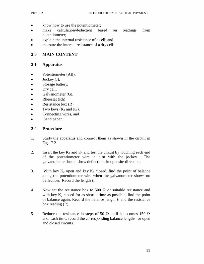
35

know how to use the potentiometer; make calculation/deduction based on readings from

potentiometer; explain the internal resistance of a cell; and measure the internal resistance of a dry cell. 3.0 MAIN CONTENT 3.1 Apparatus Potentiometer (AB), Jockey (J), Storage battery, Dry cell, Galvanometer (G), Rheostat (Rh) Resistance box (R), Two keys (K1 and K2), Connecting wires, and Sand paper. 3.2 Procedure 1. Study the apparatus and connect them as shown in the circuit in

Fig. 7.2. 2. Insert the key K1 and K2 and test the circuit by touching each end

of the potentiometer wire in turn with the jockey. The galvanometer should show deflections in opposite direction.

3. With key K2 open and key K1 closed, find the point of balance

along the potentiometer wire when the galvanometer shows no deflection. Record the length l1.

4. Now set the resistance box to 500 or suitable resistance and

with key K2 closed for as short a time as possible, find the point of balance again. Record the balance length l2 and the resistance box reading (R).

5. Reduce the resistance in steps of 50 until it becomes 150

and, each time, record the corresponding balance lengths for open and closed circuits.


36

3.3 Data Processing For each set of reading above, calculate the corresponding values of r. Tabulate your reading and calculate values as in the Table below TABLE

Table 7.1

S.No. R () l1(cm) l2(cm) r = R

2

21

lll ()

1. 2. 3. 4. 5.

Use the graphical method to obtain the value of r. Plot a graph between 1/R and 1/r using the Eq. 7.8. You know the equation of a straight line is y= mx + c where m is the slope and c is the intercept. Compare this equation for a straight line with Eq. 7.8 and determine the slope and also the intercept on the 1/r axis. Calculate the value of internal resistance. You can also determine the value of r by using Eq. (7.7). 4.0 RESULT The internal resistance of a dry cell is ….. 5.0 CONCLUSION (i) Determine the slope of the graph you have drawn and find the

value of r. (ii) Determine the value of r using Eq. 7.7. (iii) Compare the values of r obtained in (a) and (b). (iv) What conclusions can you reach concerning this experiment?


37

6.0 PRECAUTIONS Check the deflections on both sides. If it is not so, then the check

the circuit again. The battery used should be of constant emfs. The emf of the battery should be greater than the emfs of the cell. The ends of the connecting wires should be cleaned before

joining with a sand paper. The connections in the circuit should be tight and clear. The jockey should not be dragged and it should be moved gently.


38

UNIT 3 TO COMPARE EMFs OF TWO CELLS USING A POTENTIOMETER



4.0 Result 5.0 Conclusion 6.0 Precaution 1.0 INTRODUCTION In the last unit, you have learnt that potentiometer is used to determine the internal resistance of a cell. Apart from determination of internal resistance of a cell, the potentiometer can also be used to compare the e.m.f of the cells. In this experiment, you will learn to compare the e.m.f. of two cells using a potentiometer. The circuit used to carry out this experiment is given below in Fig. 8.1.

A

200

300

400

K1

E

Rh + -

B

+

-

100 50 60 70 80 90 10 20 30 40

J

A

E1

E2 + -

- +

1

2

3 K2

G

Fig. 8.1


39

The positive of both the cells, whose e.m.f.s E1 and E2 be compared, are connected to terminal A of the potentiometer and their negative are connected to two-way-key K2 as shown in Fig. 8.1. A battery E is connected to terminal B through a Rheostat Rh and a key as shown in Fig. 8.1. The e.m.f. of this battery E is greater than the e.m.f. of either of the two cells E1 and E2. Here E1 is the Leclanche cell and E2 is the Daniel cell. A constant current is passed through the potentiometer wire between the points A and B to compare the e.m.f.s of the cells. The current is kept constant by using the rheostat. This length is termed L1 when the Leclanche is used and L2 when the Daniel cell is used. The theory used for this experiment is given below. THEORY The potential difference between the points A and C of the potentiometer wire is given by P.DAC = I RAC Where RAC is the resistance of wire AC. But as you know that there is a relation between resistance and resistivity as

R = Al

Therefore,

P.DAC = IAl …………….. (8.1)

where is the resistivity of the wire and A its cross-sectional area.

Hence, P.DAC = lAI

………..………. (8.2)

That is P.DAC l (since I, , A are all constant along the wire) P.dAC = Kl………………………..…(8.3) where K is the constant of proportionality. When the key K2 is put in the gap between 1 and 3, the cell E1 come in the circuit. Let the balancing length for this cell is L1. At balance E1 = KL1 ………………………..… (8.4) Similarly when the key is put in the gap between 2 and 3, let L2 is the balancing length, then


40

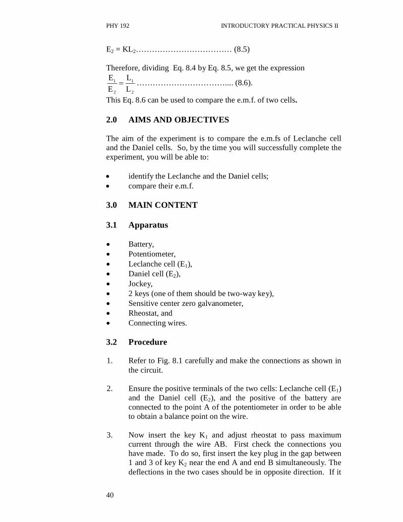
E2 = KL2……………………………… (8.5) Therefore, dividing Eq. 8.4 by Eq. 8.5, we get the expression

2

1

2

1

LL

EE

…………………………….... (8.6).

This Eq. 8.6 can be used to compare the e.m.f. of two cells. 2.0 AIMS AND OBJECTIVES The aim of the experiment is to compare the e.m.fs of Leclanche cell and the Daniel cells. So, by the time you will successfully complete the experiment, you will be able to: identify the Leclanche and the Daniel cells; compare their e.m.f. 3.0 MAIN CONTENT 3.1 Apparatus Battery, Potentiometer, Leclanche cell (E1), Daniel cell (E2), Jockey, 2 keys (one of them should be two-way key), Sensitive center zero galvanometer, Rheostat, and Connecting wires.

3.2 Procedure 1. Refer to Fig. 8.1 carefully and make the connections as shown in

the circuit. 2. Ensure the positive terminals of the two cells: Leclanche cell (E1)

and the Daniel cell (E2), and the positive of the battery are connected to the point A of the potentiometer in order to be able to obtain a balance point on the wire.

3. Now insert the key K1 and adjust rheostat to pass maximum

current through the wire AB. First check the connections you have made. To do so, first insert the key plug in the gap between 1 and 3 of key K2 near the end A and end B simultaneously. The deflections in the two cases should be in opposite direction. If it


41

is so, it means, the connections are correct. Otherwise, check again the connections or adjust the rheostat ( If there is any problem, you may consult with the facilitator.)

4. Once the connections are correct, then insert the plug of the key 2

between 1 and 3 and bring the Leclanche cell (E1) in the circuit and find the balance point and measure the length L1, that is AL1.

5. Also measure a balance point for Daniel cell (E2) and measure the

length L2. 6. Repeat the procedure four more times alternatively for the

Leclanche cell and Daniel cell respectively and enter the results in the Table 8.1 given below.

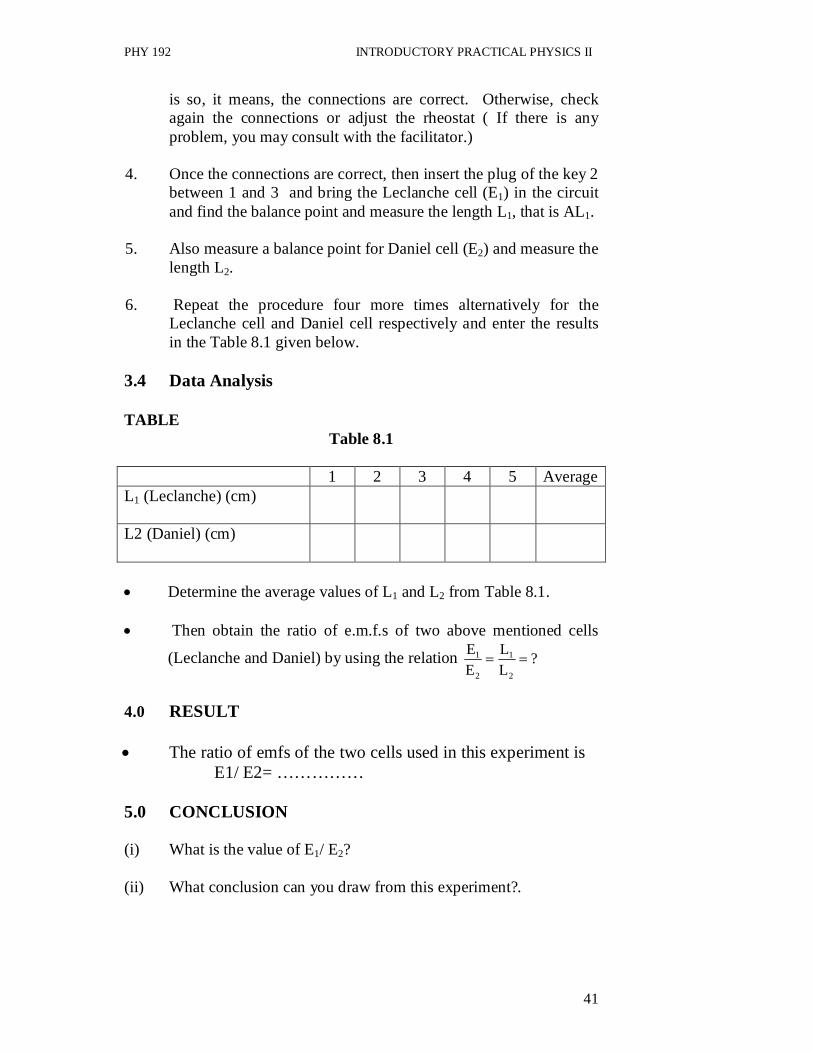
3.4 Data Analysis TABLE

Table 8.1

1 2 3 4 5 Average L1 (Leclanche) (cm)

L2 (Daniel) (cm)

Determine the average values of L1 and L2 from Table 8.1. Then obtain the ratio of e.m.f.s of two above mentioned cells

(Leclanche and Daniel) by using the relation ?LL

EE

2

1

2

1

4.0 RESULT The ratio of emfs of the two cells used in this experiment is

E1/ E2= …………… 5.0 CONCLUSION (i) What is the value of E1/ E2?

(ii) What conclusion can you draw from this experiment?.


42

6.0 PRECAUTIONS All the connections in the circuit should be tight. The e.m.f. of the battery should be greater than the e.m.f.s of

either the cells used in the experiment. The ends of the connecting wires should be cleaned before

joining with a sand paper. All the positive terminals of cell and battery should be connected

to the same end of the potentiometer. The jockey should not be dragged and it should be pressed

gently. The Rheostat used should have low resistance.


43

UNIT 4 TO DETERMINE THE UNKNOWN RESISTANCE OF A RESISTOR USING WHEATSTONE-BRIDGE



4.0 Result 5.0 Conclusion 6.0 Precautions 1.0 INTRODUCTION So far in the Module II on experiments in electricity, you have studied about the resistances and the use of potentiometer for the determination of internal resistance of a cell and to compare the e.m.f.s of two given cells. In the last experiment, you learnt to compare the e.m.f.s of a Danial cell and Leclanche cell. But in this experiment, you will learn about another instrument known as wheatstone bridge. How the wheatstone bridge can be used to determine the unknown resistance of a resistor. The metre bridge is a practical potentiometer. It is also known as ‘Slide wire Bridge’. In this experiment, it will be used to determine the unknown resistance of a given resistor. THEORY Metre bridge is a form of wheatstone’s bridge. Refer to Fig. 9.1. This figure shows four resistances R1, R2, R3 and R4, which are connected to form a quadrilateral ABCD. A cell is connected through a key to the ends A and C while the ends B and D are connected to a galvanometer G. When the potentials of the two points across which the galvanometer is connected became equal, the potential difference across these two points becomes zero and hence no current flow through the galvanometer and we get a balance point. The diagrammatic form of the wheatstone bridge is given in Fig. 9.1. At the point of balance (i.e when it shows no deflection) the potential


44

difference at B and D are the same. Hence, p.d BD = 0. Here p.d. represents potential difference. The currents in the branches are well shown in the diagram. p.dAB = p.dAD i.e. I1R1 = I2R3……………….…. (9.1) and p.dBC = p.dDC

i.e. I1R2 = I2R4……………….…. (9.2) Dividing Eq. (9.1) by Eq. (9.2), we get

The metre bridge is a practical arrangement of the wheatstone bridge as shown in Fig. 9.2. Therefore for a metre bridge, R3 is the resistance of length of wire lx and R4 is the resistance of length of wire ls. Since the resistance of the uniform wire is proportional to its length, then, the equation becomes

s

x

2

1

ll

RR

Replacing R1 by the unknown resistance X, R2 by the standard resistance S, then the above equation can be rewritten as

s

x

ll

SX ……………………..……. (9.3)

B

C A

R1 I1

I1 R2

R3

I2 I2

Key

R4

D

G

Fig. 9.1 Cell

31

2 4

RRR R


45

On rearranging the terms in Eq. 9.3, we get

X = s

x

ll x S …………..……….. (9.4)

From the Eq. (9.4), the unknown resistance can be determined, if lx and ls are known.

Thus, graph of s

x

ll against S will be a straight line graph which passes

through the origin. The reciprocal of the slope of the graph gives the value of the unknown resistance. Note that lx is equal to the effective length of bridge wire. 2.0 AIMS AND OBJECTIVES The aim of this experiment is to determine the value of the unknown resistance of a given resistor using the wheatstone bridge. Consequently, by the time you completely carryout the experiment successfully, you will be able to: recognize and know the principle behind the use of the

wheatstone bridge; use the wheatstone bridge; identify the conditions governing the use of wheatstone bridge;

and determine the unknown resistance of a resistor using the

wheatstone bridge.

3.0 MAIN CONTENT

3.1 Apparatus

Wheatstone (or Metre) bridge, Accumulator, Plug key, Standard resistance box, Resistance wire, Galvanometer, and Jockey.


46

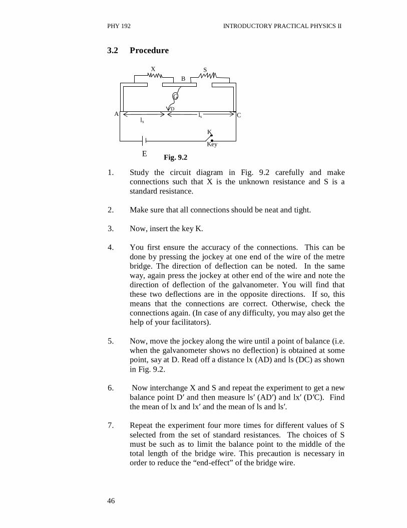
3.2 Procedure D E 1. Study the circuit diagram in Fig. 9.2 carefully and make

connections such that X is the unknown resistance and S is a standard resistance.

2. Make sure that all connections should be neat and tight. 3. Now, insert the key K. 4. You first ensure the accuracy of the connections. This can be

done by pressing the jockey at one end of the wire of the metre bridge. The direction of deflection can be noted. In the same way, again press the jockey at other end of the wire and note the direction of deflection of the galvanometer. You will find that these two deflections are in the opposite directions. If so, this means that the connections are correct. Otherwise, check the connections again. (In case of any difficulty, you may also get the help of your facilitators).

5. Now, move the jockey along the wire until a point of balance (i.e.

when the galvanometer shows no deflection) is obtained at some point, say at D. Read off a distance lx (AD) and ls (DC) as shown in Fig. 9.2.

6. Now interchange X and S and repeat the experiment to get a new

balance point D′ and then measure ls′ (AD′) and lx′ (D′C). Find the mean of lx and lx′ and the mean of ls and ls′.

7. Repeat the experiment four more times for different values of S

selected from the set of standard resistances. The choices of S must be such as to limit the balance point to the middle of the total length of the bridge wire. This precaution is necessary in order to reduce the “end-effect” of the bridge wire.

B X S

A

G

ls lx

C

Key

Fig. 9.2

K


47

During the experiment note the following: Uniformity of the wire is very important. Hence the contact

between the jockey and the wire must always be tight. Never press hard or drag the sliding contact on the wire. If a light touch is insufficient to indicate whether the balance point has been reached or not, the jockey must be cleaned and the wire may be rubbed very lightly through its entire length.

An important difference between this apparatus and the potentiometer is in connection with the source of e.m.f. In the case of metre bridge need not be constant, so that it is not necessary to use an accumulator. It is, indeed, undesirable, because no account of the low internal resistance of the accumulator is required. The Leclanche cell is preferred as its e.m.f. is high enough to give the required sensitivity and its internal resistance is high enough to limit the current to safe maximum.

The galvanometer could be damaged if too high current is passed

through it. Therefore, put a high resistance in series with this galvanometer until a rough value of balance had been obtained. This will gradually be reduced and finally removed for the final adjustment. This is the purpose of the galvanometer protector provided.

When seeking the “null” point, the key K should be closed before

contact is made at D, this is to avoid deflections due to induction effects.

The metre bridge is most accurate when the balance point is near

the center of the wire. Therefore, standard resistance should be chosen such that the balance point lies within the middle of the total length of the bridge wire.

3.3 Data Processing Your readings should be tabulated as follows:


48

TABLE Observations:

Table 9.1

S() 1x(cm) 1x (cm) Mean

1x(cm) = 2

ll xx

1s(cm) 1s(cm) Mean

1s(cm) = 2

ll ss

x

s

ll

From the values obtained in the Table above plot xlsl against S.

Determine the slope of the graph. Then determine the value of unknown resistance. 4.0 RESULT The value of a resistance obtained is …………..

5.0 CONCLUSION (i) What is the value of the slope of the graph above? (ii) What does the slope represent? (iii) Deduce the value of the unknown resistance. (iv) What conclusion can you make from this experiment? 6.0 PRECAUTIONS The jockey must be cleaned and the wire may be rubbed very

lightly through its entire length. The galvanometer could be damaged if too high current is passed

through it. Therefore, put a high resistance in series with these galvanometer until a rough value of balance had been obtained. This will gradually be reduced and finally removed for the final adjustment.


49

When seeking the “null” point, the key K should be closed before contact is made at D, this is to avoid deflections due to induction effects.

The metre bridge is most accurate when the balance point is near

the center of the wire. Therefore, standard resistance should be chosen such that the balance point lie within the middle of the total length of the bridge wire.


50

UNIT 5 EXPERIMENT TO DETERMINE THE RELATIONSHIP BETWEEN CURRENT THROUGH TUNGSTEN AND POTENTIAL APPLIED ACROSS IT



4.0 Result 5.0 Conclusion 6.0 Precautions 1.0 INTRODUCTION In the last experiment, you studied about the use of wheatstone bridge to determine the resistance of a unknown resistor. You must have seen electric bulb in your houses. The obvious question arises: How these bulbs glow? You have learnt about resistors. You know that the electric bulb (domestic or car bulb) consists of a filament. The filament of these bulbs or any type of filament is a resistor. This resistance may or may not be ohmic i.e. it may not obey Ohm’s law completely. In this experiment, we consider the tungsten filament. Now in this experiment, you will learn to determine the relationship between current through Tungsten and potential applies across it. The specific theory applicable to this experiment is briefly discussed below: THEORY The relation between the current I, through the heated filament and the applied voltage, V, is given by the general form I = KVn ……………(10.1)

Here K and n are the constants for the particular lamp. For the empirical relationship between I and V, the constants K and n can be obtained from the graph of log I against log V. Thus taking log on both sides for Eq. (10.1), we get log I = n log V + log K ………….(10.2)


51

If log I is plotted against log V, a straight line graph is obtained in which K is the intercept on the log I axis. 2.0 AIMS AND OBJECTIVES The aim of this experiment is to investigate the relationship between the current flowing through a tungsten filament and the potential applied across it. Therefore, by the time you successfully carry out the experiment, you will be able to: connect the circuit diagram; measure the current flowing in the circuit and therefore in the

filament; measure the voltage applied across the filament; plot the appropriate graph; and deduce from the graph the relationship between the current

flowing through the filament and the voltage applied across the filament.

3.0 MAIN CONTENT 3.1 Apparatus 12 volt accumulator battery, High resistance rheostat, Voltmeter, Ammeter, and 12-volt/36-watt car bulb.

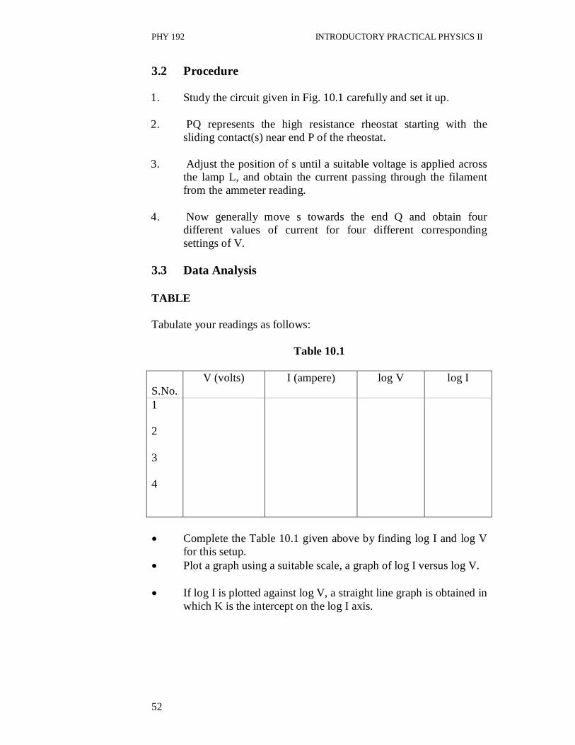
Fig. 10.1: Circuit Diagram

Q P

V

A

L Bulb

Battery

Rheostat

Voltmeter Ammeter


52

3.2 Procedure 1. Study the circuit given in Fig. 10.1 carefully and set it up. 2. PQ represents the high resistance rheostat starting with the

sliding contact(s) near end P of the rheostat. 3. Adjust the position of s until a suitable voltage is applied across

the lamp L, and obtain the current passing through the filament from the ammeter reading.

4. Now generally move s towards the end Q and obtain four

different values of current for four different corresponding settings of V.

3.3 Data Analysis TABLE Tabulate your readings as follows:

Table 10.1

S.No.

V (volts) I (ampere) log V log I

1 2 3 4

Complete the Table 10.1 given above by finding log I and log V

for this setup. Plot a graph using a suitable scale, a graph of log I versus log V. If log I is plotted against log V, a straight line graph is obtained in

which K is the intercept on the log I axis.


53

4.0 RESULT The relationship between the current flowing through the filament

and the voltage applied across the filament is ….. 5.0 CONCLUSION (i) What is the slope of the graph of log I versus log V? (ii) What is the value of log I when log V = 0? (iii) Deduce the value of K from the graph. (iv) What conclusion can you draw from this experiment? (v) Deduce the exact relationship (equation) between I and V. 6.0 PRECAUTIONS All the connections should be neat and clean. The graph should be drawn properly. The values should be chosen properly on the scale.

NATIONAL OPEN UNIVERSITY OF NIGERIA … · 2017-03-09 · PHY 192 INTRODUCTORY PRACTICAL PHYSICS II...

Documents

Transcript of NATIONAL OPEN UNIVERSITY OF NIGERIA … · 2017-03-09 · PHY 192 INTRODUCTORY PRACTICAL PHYSICS II...