U.S. DEPARTMENT OF COMMERCENATIONAL OCEANIC AND ATMOSPHERIC ADMINISTRATION

NATIONAL WEATHER SERVICENATIONAL METEOROLOGICAL CENTER

OFFICE NOTE 395

DYNAMIC COUPLING BETWEEN THIE NMC GLOBAL ATMOSPHEREAND SPECTRAL WAVE MODELS

D. Chalikov, D. Esteva, M. Iredell,and P. Long

August 1993

This is an unreviewed manuscript, primarily intended for informalexchange of information among NMC staff members

U.S. DEPARTMENT OF COMMERCENATIONAL OCEANIC AND ATMOSPHERIC ADMINISTRATION

NATIONAL WEATHER SERVICE

TECHNICAL NOTE*

DYNAMIC COUPLING BETWEEN THE NMC GLOBAL ATMOSPHEREAND SPECTRAL WAVE MODELS

DMITRY CHALIKOV, DINORAH ESTEVA, MARK IREDELL,AND PAUL LONG

AUGUST 1993

THIS IS AN UNREVIEWED MANUSCRIPT, PRIMARILY INTENDED FOR INFORMALEXCHANGE OF INFORMATION

*OPC CONTRIBUTION NO. 78NMC OFFICE NOTE NO. 395

OPC CONTRIBUTIONS

No. 1. Burroughs, L. D., 1986: Development of Forecast Guidance for Santa Ana Conditions.

National Weather Digest. Vol. 12 No 1, 8pp.

No. 2. Richardson, W. S., D. J. Schwab, Y. Y. Chao, and D. M. Wright, 1986: Lake Erie Wave

Height Forecasts Generated by Empirical and Dynamical Methods -- Comparison and

Verification. Technical Note, 23pp.

No. 3. Auer, S. J., 1986: Determination of Errors in LFM Forecasts Surface Lows Over the

Northwest Atlantic Ocean. Technical Note/NMC Office Note No. 313, 17pp.

No. 4. Rao, D. B., S. D. Steenrod, and B. V. Sanchez, 1987: A Method of Calculating the

Total Flow from A Given Sea Surface Topography. NASA Technical Memorandum 87799.,

l9pp.

No. 5. Feit, D. M., 1986: Compendium of Marine Meteorological and Oceanographic Products

of the Ocean Products Center. NOAA Technical Memorandum NWS NMC 68, 93pp.

No. 6. Auer, S. J., 1986: A Comparison of the LFM, Spectral, and ECMWF Numerical Model

Forecasts of Deepening Oceanic Cyclones During One Cool Season. Technical Note/NMC

Office Note No. 312, 20pp.

No. 7. Burroughs, L. D., 1987: Development of Open Fog Forecasting Regions. Technical

Note/NMC Office Note, No. 323., 36pp.

No. 8. Yu, T. W., 1987: A Technique of Deducing Wind Direction from Satellite Measurements

of Wind Speed. Monthly Weather Review. 115, 1929-1939.

No. 9. Auer, S. J., 1987: Five-Year Climatological Survey of the Gulf Stream System and

Its Associated Rings. Journal of Geophvsical Research. 92, 11,709-11,726.

No. 10. Chao, Y. Y., 1987: Forecasting Wave Conditions Affected by Currents and Bottom

Topography. Technical Note, llpp.

No. 11. Esteva, D. C., 1987: The Editing and Averaging of Altimeter Wave and Wind Data.

Technical Note, 4pp.

No. 12. Feit, D. M., 1987: Forecasting Superstructure Icing for Alaskan Waters. National

Weather Digest. 12, 5-10.

No. 13. Sanchez, B. V., D. B. Rao, S. D. Steenrod, 1987: Tidal Estimation in the Atlantic

and Indian Oceans. Marine Geodesy, 10, 309-350.

No. 14. Gemmill, W.H., T.W. Yu, and D.M. Feit 1988: Performance of Techniques Used to

Derive Ocean Surface Winds. Technical Note/NMC Office Note No. 330, 34pp.

No. 15. Gemmill, W.H., T.W. Yu, and D.M. Feit 1987: Performance Statistics of Techniques

Used to Determine Ocean Surface Winds. Conference Preprint. Workshop Proceedings

AES/CMOS 2nd Workshop of Operational Meteorology, Halifax. Nova Scotia., 234-243.

No. 16. Yu, T.W., 1988: A Method for Determining Equivalent Depths of the Atmospheric

Boundary Layer Over the Oceans. Journal of Geophysical Research, 93, 3655-3661.

No. 17. Yu, T.W., 1987: Analysis of the Atmospheric Mixed Layer Heights Over the Oceans.

Conference Preprint. Workshop Proceedings AES/CMOS 2nd Workshop of Operational

Meteorology. Halifax, Nova Scotia, 2, 425-432.

No. 18. Feit, D. M., 1987: An Operational Forecast System for Superstructure Icing.

Proceedings Fourth Conference Meteorology and Oceanography of the Coastal Zone. 4pp.

DYNAMIC COUPLING BETWEEN THE NMC GLOBAL ATMOSPHERE ANDSPECTRAL WAVE MODELS

D. Chalikov, D. Esteva, M. Iredell, and P.Long

National Meteorological Center, Washington, D. C.

ABSTRACT

The theory and parameterization methods of small-scaleocean-atmosphere dynamical interaction are discussed. Two

different theoretical approaches to the problem are brieflypresented. One approach follows the one-dimensional theoryproposed by Chalikov and Belevich and the other is Janssen'sextension of the Miles' instability theory. Both approachesprovide for coupling the lower portion of the marine boundarylayer, the wave boundary layer, with the underlying wavy seasurface. The results of applying simplifications of each approachto couple the National Meteorological Center global atmosphere andspectral wave models are illustrated and compared. The effects,although small, are noticeable especially in areas of high winds.

1. INTRODUCTION

The local thermodynamic interaction between the ocean and theatmosphere is one of the primary mechanisms affecting theocean-atmosphere system. Thus, the accuracy of theparameterization of this interaction determines to a considerableextent the quality of weather forecasts and climate modeling.Existing approaches to parameterize this microscale interaction donot take into account several mechanisms which influence both

media. In this paper only the dynamical interaction is discussed,that is, the momentum exchange. However, the approach presentedmay be extended to take into account the sensible and latent heatexchanges and the effects of stratification.

A major concern in the theory of the planetary boundary layer isthe establishment of an appropriate relation between the turbulentstress T (bold letters denote vector quantities), and thehorizontal wind velocity vector, u = (u,v) at an arbitrary height,

z. It is generally accepted that this relation takes the form

T = Pa Cz I U I U (1.1)

where pa is the air density, and Cz is the drag coefficient at

height z.

The value of C over land for neutral stratification depends upon

the morphological surface characteristics, usually specified by the

roughness parameter or roughness height z0, which is related to Czby

1

Cz = [ K/(ln(z/zo))] 2 , (1.2)

where K is von Karman's constant.

The roughness height over the ocean is more complex due to the

dynamics of the sea surface. It is customary to estimate zo for a

wavy sea surface with the formula suggested by Charnock (1955):

zO = m u2 /g , (1.3)

where g is the acceleration og gravity, u, the friction velocity,

and m is an empirical coefficient whose experimental value has been

found to vary from 0.01 to 0.05 (Garratt, 1977). Even though

expression (1.3) has been shown to provide a representative scale

for the roughness height over the ocean, the large scatter of the

empirical data indicates that it should be considered only as a

qualitative relationship. The large scatter is in part explained

by inaccuracies in the experimental technique, nonstationarity and

inhomogeneity of the flow, and density stratification. Scatter

may also be due to systematic deviations of the wind profile from

logarithmic which are caused by wave-produced momentum fluxes.

Finally, (1.3) appears to be valid only for a fully-developed sea

in the absence of swell.

That the roughness length over the ocean depends on sea state (wave

age) was suggested by Stewart (1967), Kitaigorodski (1968), Janssen

(1982), and Donelan (1982). The nondimensional wave age g is

defined as g = c/u, , where cp is the phase speed of the dominant

wind wave.

The variability of the wave field introduces inhomogeneities in the

surface stress over the ocean which amplifies the vertical motions

at the upper levels of the marine boundary layer. Thus, the sea

state may very well affect weather evolution and climate.

The coupling between the wind and the waves was also considered by

Jeffreys (1925), Miles (1957, 1960), Phillips (1957), Fabrikant

(1976), Chalikov (1976, 1978, 1986), Janssen (1982, 1989), and

Janssen et al. (1989). Janssen extended Miles' shear-flow

mechanism by numerical solution of the Orr-Sommerfeld-Rayleigh

(OSR) equation in tandem with a diffusion-like equation with a

diffusion coefficient dependent on the wave spectrum and solutions

to the OSR equation (Orr, 1907; Sommerfeld, 1980; Rayleigh, 1880).

Expressing Phillips' constant as a power law with strong dependence

on wave age which fits observed field wave spectra Janssen et al.

(1984) found a strong coupling between the wind and waves for young

(i.e. small wave age) wind waves, and a much weaker coupling for

older waves. Janssen's approach was applied by Weber et al. (1992)

to couple the wave model WAM (WAMDIG, 1988), to a general

2

atmospheric circulation model (ECHAM2, Roeckner et al., 1989). Inthe present study, a simplified form of the Janssen analysis isused which approximates the decrease in roughness length with waveage as found by Janssen.

Chalikov (1992) argued that Janssen's approach has somedifficiencies that precludes its confident use to model the air-seamomentum transfer. In particular, Janssen's reduction of theair-sea momentum transfer to a diffusion-like equation amounts toa diffusion equation with an advection term proportional to thevertical derivative of the diffusion coefficient. It is unlikelythat the momentum transfer may be modeled by such anadvection/diffusion process (Chalikov, 1992).

2. WAVE BOUNDARY LAYER MODEL: CHALIKOV'S APPROACH

A summary of the wave boundary layer model proposed by Chalikov andBelevich (1992) is presented in this section. Consider the bottomportion of the marine atmospheric boundary layer, the wave boundarylayer (WBL), to be a nonstationary layer with a structureapproximately governed by the equation:

au a (T + (2.1)at az-where z is a vertical coordinate which at small heights will beconsidered as a surface-following coordinate, (Chalikov andBelevich, 1992); u is the velocity vector; T and i arerespectively the vertical fluxes of momentum due to turbulenceand to wave-induced perturbations. T may be parameterized as

T M~~~ auz ~(2.2)

where K is the coefficient of turbulent viscosity. At a non-dimensional height ~ = z/Xa, the wave induced momentum flux may beexpressed as

T= l =@gS ( ( 8) P ( a C,)F( 't al) CA, E.) dd2.VA9 r 9(2.3)

where pw is the water density, g is the acceleration of gravity,and k is the wavenumber. The function F(,aICAe) describes thevertical variation of wave-induced momentum flux for eachnondimensional spectral frequency (a,

lu~~l COSO ~~(2.4)0a = 6 I Ul I coS e(24)

where uA is the wind velocity at a height z = Xa:

3

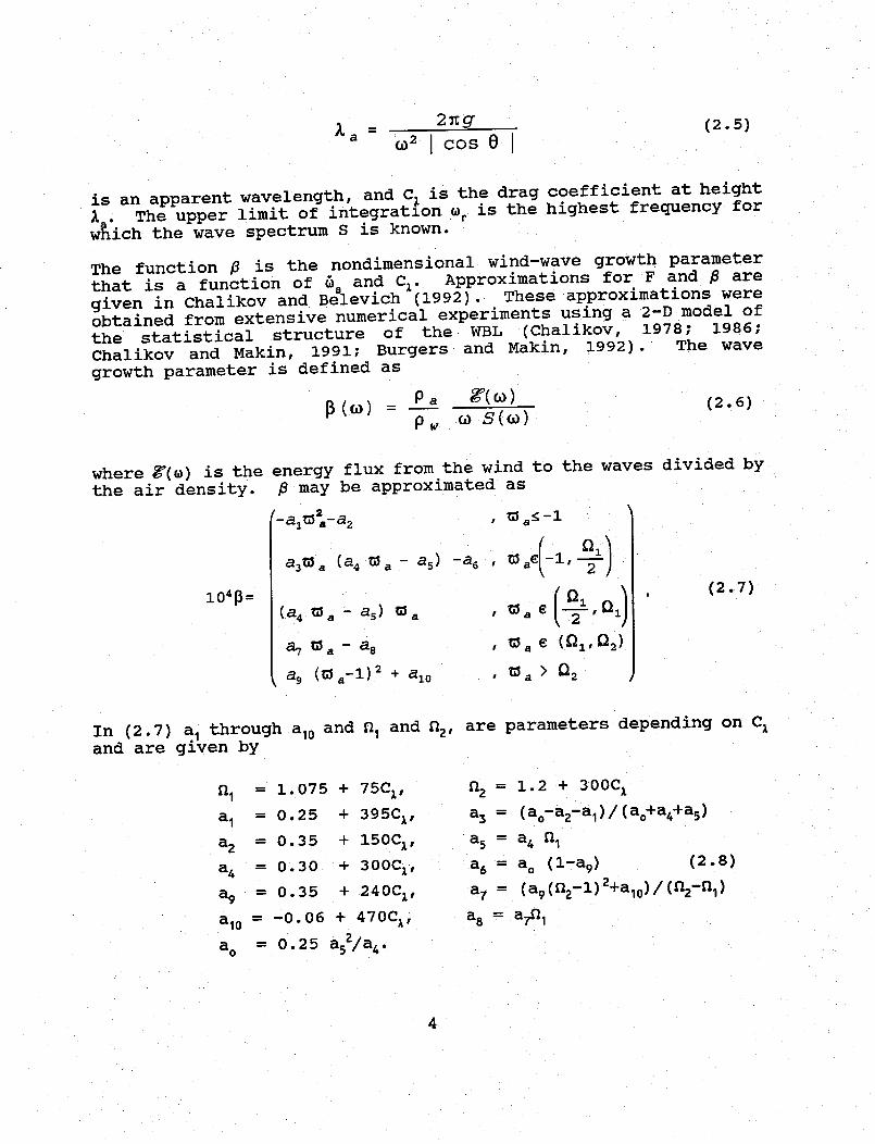
(2.5)= 2 2 g~a (D2 I C O s 0 I

is an apparent wavelength, and C is the drag coefficient at heightI. The upper limit of integration or is the highest frequency for

which the wave spectrum S is known.

The function P is the nondimensional wind-wave growth parameter

that is a function of a and CA. Approximations for F and X are

given in Chalikov and Belevich (1992). These approximations were

obtained from extensive numerical experiments using a 2-D model of

the statistical structure of the WBL (Chalikov, 1978; 1986;

Chalikov and Makin, 1991; Burgers and Makin, 1992). The wave

growth parameter is defined as

(2.6)(W) = Pa X ())p ,,, S( )

where d(e) is thethe air density.

energy flux from the wind to the waves divided byP may be approximated aswhere g(U) is the~~~~~~

( -alt3Sa-a 2

a 3t13 (a4 Wa - as)

(a 4 t5 - as) a

a7 va - as

a9 ( a-1l) 2 + a10

· was -1

I

-a6 , ae(1 32

I ~~2 > ( 2a )

, lo a e (all 2)

ti5 , > Q2 /

(2.7)

In (2.7) a1 through a10 and E1 and E2, are parameters depending on Cand are given by

n = 1.075 + 75CA,

a, = 0.25 + 395CI,

a2 = 0.35 + 150CI,

a4 = 0.30 + 300C1,

a9 = 0.35 + 240CI,

a10 = -0.06 + 470Cr,

ao = 0.25 a52/a4

·

n2= 1.2 + 300Cx

as = (ao-a2-a1l)/(ao+a4+a5)

a5 = a4 (1

a6 = ao (1-a9 ) (2.8)

a7 = (a9 (n 2 -1) 2+a10 ) / (nz-fl1 )

a8 = a71

4

For frequencies Ila.1 2 2 the parameter 6 depends on &a2 and,therefore, on the square of the wind speed. This dependence isconfirmed by the experimental data of Hsiao and Shemdin (1983), andis more representative than the linear dependence derived from thefield data of Snyder et al. (1981). High frequency waves arenearly stationary relative to the wind; thus, their drag inturbulent flow is likely to have a quadratic dependence on windspeed, as is the case for stationary roughness elements. Thelinear dependence of P on &a exists only for .a e (l , n2) . For &< -1, P becomes negative. This case corresponds to waves travelingagainst the wind, and suggests that in this case the waves transferenergy to the wind. This is referred to as the inverse Miles'mechanism. The use of u, and C; above eliminates the arbitrarinessin choosing a reference level. It also reduces the number ofgoverning parameters and is physically more meaningful because thethickness of the WBL decreases with frequency. The approximations(2.7) and (2.8) are also confirmed by Plant's (1982) data,including the quadratic dependence of P on 1a for lIaI > 2 (Fig. 1).The considerable scatter of Plant's data may be due to theadditional dependence on C.

Construction of a 1-D model of the WBL requires a definition of thevertical distribution of the wave-induced momentum flux T in (2.1).For a monochromatic wave traveling at an angle 0 to the wind, thisis

= T o F(u al CA,) , (2.9)

where To is the wave-induced momentum at the surface. The form ofthe scalar function F was investigated in numerical experimentswith a 2-D model (Chalikov and Makin, 1991). An approximationbased on the work of Makin (1989) is

F= [1 - ]e10 (2.10)

where EO is a function of the drag coefficient C,

O = 0.1 + 60Cx.

Thus, in practice F is independent of &a The wave frequencyinfluences the wave momentum flux at the surface, but not itsvertical distribution. In the case of a multi-mode wave surface,it is assumed that T is the superposition of the fluxes due to allspectral components.

The coefficient I, in (2.2) may be computed from

KM= Kz( e/c) 1/2 (2.11)

5

where c1 is a constant equal to 4.6, and the turbulent kinetic

energy e may be computed from

ae = [KM au + ] a. 3 (2.12)

at az az Kz

In (2.12) the effect of diffusion of turbulent kinetic energy is

not included since it is usually small; the dot denotes the scalar

product.

The model formulated above illustrates the general approach to be

used when modelling the WBL-wave field system. The time and space

evolution of the wave field may be simulated by a spectral wave

model. The coupling of the two systems is accomplished through

the exchange of information between the WBL and wave models. The

WBL model computes and transfers to the wave model the spectral

energy density input to the waves. The wave model computes the

evolution of the wave spectrum in time and space and transfers the

"sea state" to the WBL model. Equations (2.1) through (2.12)

constitute a 3-D model describing the evolution of the atmosphere-

wave coupling. These equations establish the connection between

the turbulent stress and wind in the lowest layer of the

atmosphere. The updated stress components are then used in the

next time step.

The time scale Ts for the WBL processes may be estimated from

TS = h/(AC z U), (2.13)

where h is the thickness of the layer, and ACzis the change in the

drag coefficient due to the influence of the waves. Since ACz is

of the same order of magnitude as Cz, that is, ACz 10'3, T_ is on

the order of 3 x 103s. The time step for a 3-D atmosphere model is

on the same order of magnitude; therefore, it is reasonable to use

the stationary version of the WBL equations:

a (T+) = 0 (2.14)az

au + * au KM = (2.15)[Kmaz az (KZ)4(Kz)

Equation (2.14) may be written in the form:

T + T = Th , (2.16)

where Th is the constant of integration, which equals the stress

vector above the WBL. Then (2.15) may be written:

6

Tba ( - 0 (2.17)az (KZ) 4

which may be rewritten as

(KZ) 4/ 3 (h aU ) 1/3 U (2.18)az Taz

Since Th is unknown, two boundary conditions are necessary to solve(2.18). The first is the prescribed velocity vector at height h,

z = h: U = U.1 (2.19)

The second is the expression for the tangential stress vector atthe water surface,

Zr: Km - pa (2.20)Z r KMLZ P a Cr |U X I U.:Z.o

The lower boundary height Zr is prescribed by the cut-off frequency

Or:

2 7cgz = (2.21)

It is assumed that the lowest part of the WBL is responsible forthe creation of the local tangential stress due to waves withfrequencies ( > or. Waves with frequencies X < er give rise toadditional form drag which is taken into account in the integral(2.3). Assuming the Phillips' spectrum is valid for frequenciesgreater than r:

(0 > r: S((O) = ag 2 W- 5 (2.22)

and that the local roughness 0 due to these waves is determined bytheir height, Chalikov and Belevich (1992) estimated

2

c 1-/2 (2.23)9-

° g

with X = 0.1. Averaging the wave spectrum at o=or over all angles:

S f )' S(2 r ,) , (2.24)

and equating this average to the Phillips' spectrum for X = or

7

S(() = S( r)( ) (2.25)

(2.23) takes the form

2

= X 2 [S (G r) ] 1/2 Xs/2 (2.26)

The local drag coefficient is then given by

Cr = [K/(ln (zr/4) ) (2.27)

An effective roughness parameter may then be found by combining

(2.26) and the solution of (2.3). An approximation to this

effective roughness is given in (2.31) below.

Equation (2.18), with boundary conditions (2.19), (2.20), and

formulas (2.3) - (2.5), (2.7), (2.8), (2.10), (2.21), (2.26), and

(2.27) formulate the parameterization of the WBL for use in

coupling the atmosphere-wind wave system. Note that the integral

in (2.3) depends on the vertical distribution of the wind u(z) and

the drag coefficient Cz, which by definition is

CZ= T I / u(z) 12 (2.28)

For the numerical solution of (2.18) it is necessary to evaluate

(2.3) by iteration. The values for Cz and u(z) may be obtained

from a linear interpolation of the logarithmic scale

1n= ln(z/zr)

which, in practice, is convenient to use in the numerical solution

of (2.18).

The approach presented above, although not overly complicated,

takes a considerable amount of computer time. In the preliminary

experiments discussed in this work, several simplifications were

adopted: first, it was assumed that the spectra generated by the

wave model includes the locally generated wind waves, which may be

approximated by the JONSWAP spectrum (WAMDI group, 1988). The rest

of the spectrum is considered to be swell and assumed not to

contribute to the wave-induced momentum flux. This assumption,

should not introduce large differences since the swell contribution

to the wave induced momentum should be small due to the small

steepness of these waves.

8

It was assumed that the spectral peak in the spectra generated bythe wave model closest to the local wind corresponded to thelocally generated wind sea. The frequency of this peak wasdetermined by minimizing the expression

(kx - kxr) 2 + (kyi - kyr) (2.29)

where kxi, k.n are the x,y components of the wave number for spectralpeak i, and kxr, kyr are those of the wave number of the shortestrepresented wave, which is assumed to be in the direction of thewind. Minimizing (2.29) is equivalent to minimizing

4+ 4- 2)2( rCOS(i Ow) (2.30)

in frequency-direction space. m) and 0. are the frequencies anddirections of the different peaks, 0w is the wind direction, and ris the frequency of the shortest wave represented in the spectrum.Once the frequency of the local wind wave is selected, itscorresponding phase speed is used to determine the inverse waveage, and the effective roughness height z0 is computed from

z0= (u2 /g)exp(-11.35+0.187R+(0.84+0.065R) (u/cp))

with R = ln(u2/(gz)).

Equations (2.7) and (2.8), were not introduced. Only the large-scale coupling between the atmosphere and the waves has been,considered, hence equations (2.7) and (2.8), were not introduced.

3. SHEAR FLOW MECHANISM: JANSSEN'S APPROACH

The theory of wind generated gravity waves as presented by Miles(1957, 1960, 1976) is similar to the theory of the resonantinteraction of plasma waves with particles (Landau and Lifshitz,1954; Fabrikant, 1976). Surface waves in plane-parallel flow aregenerated with phase velocities equal to the wind velocity at some"critical" (or resonant) level, zc. Depending upon the influenceof the wave age on the Phillips' parameter in the wave spectrum,the wave-induced stress can be a significant fraction of the totalstress (Janssen et al., 1989). For waves traveling along the meanhorizontal wind u, and subject to certain conditions, Janssen(1982) has shown that the wind-wave interaction may be modeled bya diffusion-like coefficient, D,(k,z),

Dw(k,z) = 2k ¢(k) Ix(k,z) 12. (3.1)C - Vg

9

In the treatment that follows, vector notation will be dropped

since it is assumed that the waves are aligned with the mean wind.

Together with turbulent and viscous stress, the mean wind satisfies

the equation,

au/at = a 2 u + 1 aT + Dw(kz) (3.2) pau (3.2)az2 p azz - -

in which T is the turbulent stress which is assumed to be modeled

by a mixing length theory.

In (3.1, 3.2), vg, 0 (k), va, D (k,z), and x(k,z) denote: the group

velocity of a surface wave with wave number k and phase speed c,

the spectral amplitude, the molecular viscosity of air, the

diffusion-like coefficient that models the air-sea interaction, and

the normalized solution of the OSR equation, respectively.

The Orr-Sommerfeld equation is a 4th-order ordinary differential

equation:

xiv_ 2k2X" + k4X = ikRe[(u - c) (X! - k2X)-u!x] (3.3)

in which Re is the Reynolds number. If Re is taken to be infinite,

then

2 - k2X U X = 0 , (3.4)dz2 U - C

which is the OSR equation. For the MBL, the boundary conditions

for (3.4) are

X (z - 0) = 1

(3.5)x (z -* co) = 0

The function X(z,k) arises from a perturbation solution to a

plane-parallel flow as follows. Let the nondimensional

Navier-Stokes equation be expressed in terms of a mean and a

perturbed flow:

p = P + p/

(3.6)U = U +u

W = W/

10

az

w/ = aX (3.7)ax

then

a2 + u, aU au a ap + j .a* oazat axaz az ax ax Re az

___+ 12 apl + Va~ + U X-t a px+ a (3.8)

axat ax 2 az Re ax

where primes indicate perturbed quantities. Using the separationof variables technique with trial solutions

(x,z,t) = X(z)exp[ik(x-ct)]

p/(x,z,t) = I[(z) exp[ik(x-ct)] (3.9)

results in (3.10), and (3.11) below.

ik(U-c) dA -ik dU X = -ikI + ( - k d (310)dz dz Re dz 3 dz (3.10)

k2(c-U)X- d= M ik d2X k2) (3.11)dZ Re dz2-

Equations (3.10) and (3.11) are a coupled system from which 1(z)may be eliminated to get (3.3) and (3.4).

The Rayleigh equation, (3.4), has a singularity at the criticalheight, z . Since (3.6) - (3.11) are nondimensional, X(z,k) isnormalized. The steps used by Janssen to solve the precedingequations and estimate the wind-wave interaction are givenschematically in Appendix A.

For a wave spectrum O(k,O,t), Janssen (1991) gives thefollowing

11

D (k,z)= f dO 2 I X 1 (k, 0, t)cos 20 (3.12)

in which 0 is the angle between the wind and the spectral wave

component.

A simplified version of Janssen's approach is used in this work.

The simplification consists in deriving a generalized Charnock's

constant as a function of wave age using Janssen's analysis. This

generalized Charnock formula is then used to compute the roughness

height z0 corresponding to the wave age M as determined from the

frequency fp and wave number kp of the "sea" spectral peak:

= C/u*, with c = g/kp.

This leads to a wave age dependent drag coefficient Cz.

This roughness height is passed from the wave model to the

atmosphere model which then generates the winds which will drive

the wave model for the next time step. In this fashion a two-way

coupling between the wave and atmosphere models is achieved.

The generalized Charnock relation is derived from the family of

curves adapted from Fig. 3 of Janssen (1989) (shown here in Fig.

2). These curves represent typical nondimensional velocity

profiles with and without wave perturbed flow. In the figure the

nondimensional velocity u(z)/u, is plotted versus the

nondimensional height zg/u,2. The curves are nearly straight and

parallel for zg/u z2 > 1. For zg/u,2 < 1 the perturbed curves deviate

from log-linear, and, given boundary condition (A.3), cross the

u/u* = 0 intercept at zg/u*2 = m = 0.0144. The extrapolation is not

shown in the figure.

Fig. 7 of Janssen (1989), shown here as Fig. 3, shows the

dependence of Cz at a 10 m height on wave age for two values of u,

(0.3 m/s and 0.7 m/s). Curves are shown for both the -2/3 and the

-3/2 power laws for the Phillips parameter (see Appendix A). It

can be seen that there is considerable variation of C, with wave

age for the -3/2 power law. This power law was used in obtaining

the curves in Janssen's Fig. 3.

The simplification used in this work was suggested by Fig. 2. For

zg/u*2 > 1 the curves are merely displaced from the straight line

representing the uncoupled wave-atmosphere situation. This

suggests that a general equation for the family of curves may be

written as:

12

(3.13)u(z)/u* = A ln(zg/u2) + B(p)

where A is the slope of the family of curves, and B(A) depends on

wave age only. An average value of A is 2.46.

Equation (3.13) is rewritten as

u(z) /u* =A ln [zg/D(V)u~] (3.14)

in which

B(p) = -A ln[D(p)] , (3.15)

thus,

C 1/ -2 = u(z)/u. = A ln[ (1/Cz) (zg/D(p) u2)] (3.16)

In similar fashion the Charnock relation (1.3) may be written

Cz 1/ 2 = K -1 ln[(1/Cz ) (zg/m u2 )] . (3.17)

Comparing (3.16) and (3.17) suggests:

A = K 1, (3.18)

andD(A) = a generalized Charnock "constant" (3.19)

which approaches m for large values of g.

From (3.16) through (3.18), the generalized Charnock "constant" is:

D(>) = (zg/u2) [C 1 exp(-0.407CC /2 )] · . (3.20)

Computing the D(p) for different values of wave ages yields

A 5I _ 10 1 15 20 _25

D(,!) 0.210! 0.727! 0.414! 0.0328! 0.02771

A rational fraction that approximates D(p) for A > 3 is given by

D(p) = (-0.153 - 0.00245[)/(1 - 0.358p) (3.21)

13

This approximation for D(y) is used to generalize the Charnock

relation:

= D(p) (u2/g)zo = D ([) (,/g).-

4. THE NMC ATMOSPHERE AND WAVE MODELS

Brief descriptions of the NMC atmosphere and ocean wave models are

given below. Operationally these models run independently of each

other, with the wave model using the output wind fields from the

atmosphere model as the sole input. The operational wave model

runs twice daily at the 0000 and 1200 UTC cycles. A so-called wave

analysis is generated by running a 12-hour wave hindcast, that is,

using the final analysis wind fields. This "wave analysis"

provides the initialization wave field for a 72-hour forecast. The

input wind field to the wave model is the lowest sigma layer winds

reduced to a 10-m height assuming a logarithmic wind profile. For

the coupling experiments the wave model was modified to take the u*

field directly from the atmosphere model. The runs were done once

daily, for the 0000 UTC cycle only, thus initialization wave fields

resulted from a 24 hour hindcast. The hindcast was done by running

the NMC Global Data Assimilation System (GDAS) for the preceding 24

hours with the same coupling technique as for the forecasts.

4.1 The NMC atmosphere model

The operational NMC Medium Range Forecast Model (MRF) is used for

the GDAS, the Aviation (3 day) forecast, and for the 10-day

forecast runs. The MRF is a spectral model and is described in

some detail in Kanamitsu (1989), and Kanamitsu et al. (1991). A

few of its properties are described here.

The MRF forecast variables are vorticity, divergence, virtual

temperature, specific humidity, and surface pressure. The model

variables in the horizontal are represented by spherical harmonics.

The model has 18 levels in the vertical and a horizontal

resolution of triangular truncation 126 (T126). This truncation

corresponds to a horizontal spatial resolution of approximately 105

km. However, in order to save computer time, the coupled

atmosphere-wave experiments described here were performed with a

triangular truncation of 62 (T62), which corresponds to a spatial

resolution of approximately 210 km.

The lowest layer of the atmosphere model, the surface layer, is

well defined with a height of 5 hPa (about 40 m) above the surface.

The physics in this layer is governed by surface layer Monin-

Obukhov similarity theory and improved land surface evaporation.

The atmospheric boundary layer (ABL) in the MRF consists of the

bottom surface layer and those layers above it which are influenced

14

by the turbulent transfer of momentum, heat, and moisture from thesurface layer. During vigorous daytime turbulent convection theABL is typically 1 - 2 km thick. However, during extremely stableconditions, such as may occur at night, turbulence may become soweak and irregular that it may not be possible to determineaccurately the height of the ABL. For these conditions, the ABLmay recede into the surface boundary layer. The MRF makes noprovision for this occurrence.

The MRF computes the surface turbulent fluxes of momentum, sensibleheat, and latent heat. The heat fluxes are required for thesolution of the heat balance equations that predict the air-groundinterface temperature. This heat balance calculation is omittedover the oceans although it is important in predicting theevolution of the MBL. The surface fluxes of momentum and heat areused as boundary conditions for the diffusion equations whichsimulate the turbulent transfer of these quantities above thesurface layer.

The calculation of surface fluxes in the MRF depends on thenondimensional variable zs/L, where zs is the height of the surfacelayer and L is the Monin-Obukhov length, the sign and magnitude ofwhich determines the stratification/stability of the surface layer.

The vertical profiles of (virtual) potential temperature e,specific humidity q, and wind speed in the surface layer are givenby

a- z WT(P/L) (4.1)az K

az =k P q(z,L) (4.2)az Kz

au u.auU- au u(z/L) (4.3)

-~~~ - kH ~~~~~(4.3)az Kz

(U2Ou~with L= KgO.

0*, q*, and u* are the scaling factors for heat, moisture, andmomentum. The functions (T qu are the Obukhov functions which havebeen determined empirically.

15

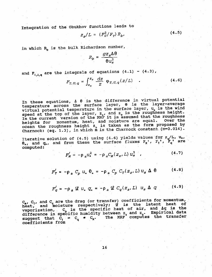
Integration of the Obukhov functions leads to

zs/L = (Ft/FT) Rb,

in which Rb is the bulk Richardson number,

gzsA OoRb- U

2

and FTUq are the integrals of equations (4.1) - (4.3),

FT U'q = z dz (PT, uq(Z/L)Z

(4.5)

(4.6)

In these equations, A 8 is the difference in virtual potential

temperature across the surface layer, 0 is the layer-average

virtual potential temperature in the surface layer, us is the wind

speed at the top of the layer, zs, and zo is the roughness height.

In the current version of the MRF it is assumed that the roughness

heights for momentum, heat, and moisture are equal. Over the

ocean the roughness height zo is taken as the form proposed by

Charnock: (eq. 1.3), in which m is the Charnock constant (m=0.014).

Iterative solution of (4.5) using (4.6) yields values for zs/L, u.,

0., and q,, and from these the surface fluxes FM ', FT', Fq' arecomputed:

FM =2) U2F;M = -P aU* = -PaCm(zs,L) us

FT = -P a Cp U* e* = -p a Cp CT(Zs, L) us A 0

(4.7)

(4.8)

Fq = Pa S u* q. = Pa S Cq(ZsiL) us A q (4.9)

C., CT, and Cq are the drag (or transfer) coefficients for momentum,heat, and moisture respectively; 9 is the latent heat of

vaporization, C is the specific heat of air, and Aq is the

difference in specific humidity between z and zo. Empirical data

suggest that CT = Cq ~ CM. The MRF computes the transfer

coefficients from

16

U,/2' K2

( ) M ~ 12 (4.10)M~us FMf

U, O, U, q9 = K2 / <2

CT = Cq =u A = uA q FF FFq . (4.11)

For the special case of neutral static stability, the transfercoefficients become

K2CM = CT = Cq = n 2 (z s / z o) (4.12)

1n2 (z,/z0 )

4.2 The NMC global wave model

The operational NMC global ocean wave (NOW) model is a deep waterspectral model with a 3 hour time step and a 2.5 by 2.5 degreelatitude-longitude grid. It produces forecasts every 3 hours from70°S to 75°N. The model solves at each grid point over the oceanthe energy transport equation:

aS + cg'VS = Sin + Snlat g

where S = S(f,8) is the two dimensional wave spectrum as a functionof frequency f and direction 0, c is the group velocity, and theterms on the right-hand side are thae source terms representing thewind input and the nonlinear wave-wave interactions.

The wind input source term follows the parameterization of Snyderet al. (1981), Sin = 'eS with the wind wave growth parameter givenby:

g' = max[0, 3 x 10-4 (30u.g-'lcosS-1) ] , (4.13)

where X is the radian wave frequency and 0 is the angle between thewind and the wave directions.

The nonlinear source term is based on the SAIL II mechanism(Greenwood et al., 1985), and is given by

SnL = ½ C z 1 u 1 02 (4.14)

where 0 is the Phillips' fetch constant (0.8 x 10-4 < < 1.6 x 10 4).

A cos3 0 law is used for spreading the energy over direction 0.Dissipation at high frequencies is accomplished by imposing the

17

Pierson-Moskowitz limit for a fully-developed spectrum (Pierson and

Moskowitz, 1964).

The propagation scheme is a downstream interpolation in which each

frequency-directional band is propagated at the group velocity

along a great circle. Upwind swell is attenuated using an

exponential attenuation term with maximum attenuation in the

direction opposite to the local wind and decreasing angularly on

either side to unity at 90 degrees.

5. COUPLING PROCEDURE

As indicated in sections 2 and 3 the procedure followed for

coupling the two models was the same for the simplified Janssen

(JS) and the Chalikov (CS) schemes.

To initialize the two-way coupling the 0000 UTC operational wave

analysis and the GDAS u, fields were used. The u. field was

transferred to the wave model and z0 values were computed using the

given u* field and the phase speeds from the wave spectra. The

computed zo field was transferred to the atmosphere model. Both

models were then advanced 3 hours, the atmosphere model now using

the wave age dependent zo field in the Monin-Obukhov formulation.

Starting with the next time step the wave model received a us field

resulting from taking the wave age dependence into account. The

procedure was then repeated. Every 24 hours a 120-hour wind

forecast and a 120-hour wave forecast were started from the GDAS

and wave hindcast fields. The exchange between the two models

continued during the forecasts runs in the same fashion as for the

hindcast (Fig. 4). The method for computing roughness over land

remained unchanged.

In parallel with these runs the atmosphere and wave models were run

without the two-way coupling, to serve as the control run. The

resulting forecasts from the control and the coupled runs were

compared.

The coupled runs using the JS approach for the nine consecutive

days starting on December 26, 1991 are compared here with those

using the CS approach for the eight consecutive days starting on

January 24, in order to have about the same number of days using

each approach.

6. RESULTS

Since the runs with the two approaches were done for different

time periods, the results are not conclusive, for the synoptic

conditions may have been different during the two periods. The

effects of the coupling will depend on these conditions. As would

be expected in the case of the waves, larger differences between

the coupled and the control runs were observed in areas of strong

winds where young seas would be expected. In the following two

18

sections typical results from both schemes will be given.

The impact on the waves was characterized by the difference insignificant wave height (SWH) between the coupled and thecorresponding control run. Impact on the wave spectra was alsoobserved. However, the impact on the wave spectra could not befully evaluated because spectra were saved at only a few locationsaround the continental United States.

6.1. IMPACT ON THE ATMOSPHERE MODEL

The largest impact on the atmosphere model during the model runsusing the JS was for January 8th. Thus the results on this datewill be discussed.

As can be seen from Figs. 5a and 5b, the JS increases the upwardlatent heat flux. The largest absolute difference between the twofields is approximately 73 watts/m2 and is located off thenortheastern coast of the United States. This location is also thesite of the strongest upward sensible heat. A lesser differencewas observed in the sensible heat fluxes (not shown). Thus itappears that the latent heat fluxes are more sensitive to thecoupling than the sensible heat fluxes.

No impact was noticeable in either surface stress or the 10-m windvectors. However, an increase in roughness height was observedover much of the ocean, as seen in Figs. 6a and 6b.

As will be discussed in section 6.2, the largest impacts on thesurface ocean waves during the period January 24 to January 31using the CS were observed for the forecasts starting on January30th. Thus, the impact on the atmosphere model for this day willbe discussed.

A slight decrease in the upward latent heat fluxes is noticed(Figs. 7a and 7b), while there is a slight increase in the upwardsensible heat fluxes as well (Figs. 8a and 8b).

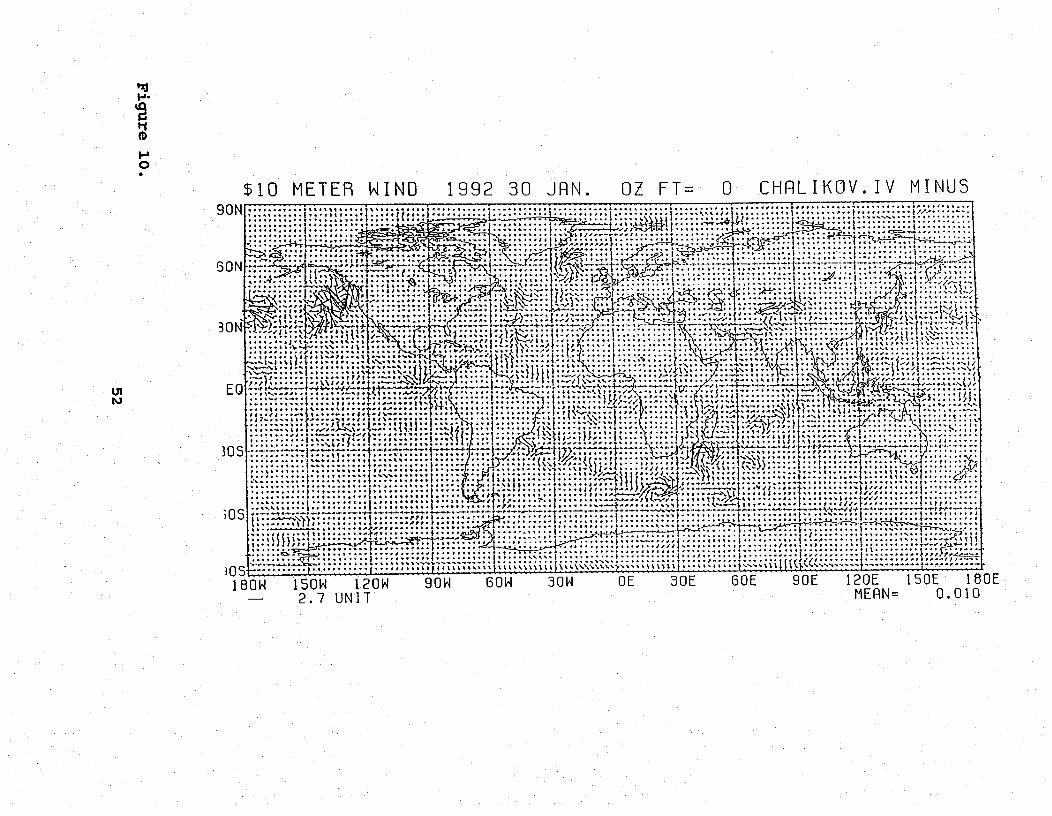
Larger differences are seen in the surface pressure forecasts, witha maximum decrease of approximately 2.9 hPa off the west coast ofthe United States, near the Canadian border. At this site thelargest differences in the surface stresses, Fig. 9, and in 10 mwinds, Fig. 10, are also noted. No roughness height fields areavailable for this case.

6.2 IMPACT ON THE WAVE MODEL

The effect of the coupling on the wave field will depend on thelocations of active wave generation and on the pre-existing waveconditions. Since the two experiments were run for different timeperiods it is not possible to arrive at definite conclusions.However, the results presented in Tables 1 through 4 suggest that

19

the CS is more consistent and produces larger impact on the waves

than the JS.

The tables give the distribution of differences in SWH between the

coupled and control runs in different regions where the larger

impacts were observed. Shown are the distribution of differences

for successive 12-hour and 96-hour forecasts (the 120-hour

forecasts could not be retrieved from the tape archive). A

tendency for the range of differences to increase with time into

the forecast can be seen.

For both approaches the impact of the coupling on the waves tends

to increase with time (successive 12-hour and 96 hour forecasts)

and with the forecast hour (12-hour forecasts versus 96-hour

forecasts). The tendencies are more pronounced for the CS than for

the JS.

The wave forecasts starting from 0000 UTC on January 30 are among

the ones showing the larger impacts of the CS coupling. Figs. 11

a and b show contours of differences in SWH between the coupled and

the control run for the 12-hour forecast in the North Pacific. The

dashed contours indicate negative differences: coupled minus

control. From Fig. 10 for the differences in the 10-m winds at

0000 UTC that day, it can been seen that the areas with reduced

SWH's correspond approximately to areas with the larger differences

in the 10-m winds. These areas are also those with the highest

winds.

The 10-m winds are not available for 0000 UTC on February 3, 1992,

but the difference contours of SWH for the 96-hour wave forecast

valid at the time show significant differences off the northwest

coast of the United States and Canada.

In contrast, the 10-m wind differences in the North Atlantic for

0000 UTC, January 30 are not as pronounced as those off the

northwest U.S. and Canadian coast, and neither are the differences

in SWH for the 12-hour forecast as seen in Fig. 11 b. The

differences in SWH in the western area of the North Atlantic

increased significantly for the 96-hour forecast (Fig. 12 b).

A slight increase of energy in the high frequencies and a

broadening of the spectra were detected in the directional spectra

for the coupled runs. Slight changes of a few degrees were noticed

in the wind direction. These changes in wind direction appear to

have an effect on the spectra for the coupled runs.

One location where spectra were saved and where significant

differences in SWH occurred was at 45°N-1300W. Figs. 13a and b

show the directional and frequency spectra at this location for the

96-hour forecasts valid at 0000 UTC on February 3, 1992. Fig. 13a

shows the spectra for the control run and 13b for the CS run. The

coupling reduced the SWH by 1.5 m, the u, by 0.11 m/s, and there

20

was a change in wind direction of 6.7 degrees. The directionalspectra show a change in the location of the spectral peak alongwith a broadening and flattening of the spectrum. The spectralpeak is better aligned with the wind direction. It is noted thatthe wave model often overpredicts the SWH in this region. The CSin general reduced the SWH, which appears to be a step in the rightdirection.

7. DISCUSSION

The two methods presented here are conceptually different. TheChalikov approach proceeds from numerical solutions of theequations of motion and numerical computations of the verticalfluxes due to turbulence and wave induced perturbations; theJanssen approach is posed as a classical instability problem.

Simplifications have been made to both these approaches in applyingthem to couple the two models. These simplifications may in partbe responsible for the small impacts obtained.

From the tables and figures given here it can be seen that theimpact of the coupling for both methods is noticeable only in smallareas of high wind speeds. This alone may be significant,especially when considering hurricane/typhoon models.

It is noted that the Chalikov approach in general reduced waveheights thus increased the roughness height. On the other hand forthe Janssen case, the occurrence of increased wave heights washigher than that of decreased wave heights.

A more sophisticated treatment whereby the wave-generated momentumflux is transferred to the atmosphere model may be more revealing.Continuation of the experiment for a longer time period especiallyduring the southern hemisphere winter would be desirable.

Acknowledgements. The authors wish to express their thanks toRachel Teboulle for developing the graphics and for helping withthe compilation of statistics between the coupled and control runs.Their thanks also go to Hann-Ming Juang and Masao Kanamitsu fortheir help.

21

APPENDIX A

In order to solve the Rayleigh equation coupled with a

diffusion-like equation and to estimate the wind-wave interaction,

Janssen used the following steps:

a. Assume the unperturbed wind profile is

(A.l)

b. Solve (3.4) with boundary conditions (3.5) for a given

k = 6Z/g.

c. Construct an extended diffusion-like equation:

au (K_ az au )+[v a+Dw(kz)] az2U-at az - - (A.2)

where the mixing length hypothesis is used for the turbulent

diffusion.

d. Solve (A.2) as an initial value problem with boundary

conditions:(A.3)u(z=z,0 1 t) =0 ; z o = (m/g) u,

where the expression for zo is the Charnock relation (1955), and

limK 2 Z 2 au au 2lim K az z = u*

z -+o

(A.4)

until u(z,t) reaches a steady state.

e. Repeat steps a-d iteratively until u(z,t) and Dw do not change

substantially.

The wave induced stress is then computed from:

lv(z=0) = -[3 aJ dzDw (k, z) a 2uIr W Z 0) -P O IWaz2 (A.5)

On the basis of wave breaking and dimensional grounds, Phillips

(1958) proposed the spectral form

22

.

(Kz )(Zo

¢(k) = 2 apk4 k kp2

4(k) = o k<kp (A.6)

where a is Phillips' parameter or "constant", and k is the wavenumber of the spectral peak. For the spectrum 0 in (3.1), Janssenassumed the JONSWAP mean spectrum for a growing sea, (Hasselmann etal., 1973):

-3 5 kp 2 r (A.7)(k) = a p k 3 exp (k)] (A.7)

kl/2 1/2 12 2r = exp - [( - k 2)/o kP]2 (A.8)2

where y = 3.3, and a = 0.1.

Empirical data suggest that the Phillips' parameter depends on waveage. Based on some field and laboratory data, Snyder (1974)proposed:

-2/3air) = bi t (A.9)

with b a constant. Janssen showed that this form yields a waveinduced stress nearly independent of wave age. A better fit tofield data is given by

=0.57 (Cp- 3/2 (A.10)

(Janssen et al., 1984). Using this power law, Janssen found afairly pronounced dependence of wave-induced stress on wave age.

23

APPENDIX B

For completeness, an approximate solution to (3.16, 3.17) is given

here. Let us define the generalized Froude numbers, Fr:

Fr = D(F) (u2/zg) or mu2 /zg

so that(B.2)C/2 = -K/ 1n ( CMFr)

CM is an implicit function of Fr; given Fr, CM can be computed by

iteration. A more direct approach is to compute CM for several

widely separated values of Fr and then to use an interpolation

approximation such as,

CM(Fr) [ (6.283 + 0.2077 x) / (1-0.6448X)]x10-3 (B.3)

where x = lnFr, and -13.4 < x < 0.94.

Another approximation is suggested by (3.17). Let C. be

approximated on the right-hand-side of (3.17) by a constant CO.

Then,

CMK2

(lnFr +lnCo ) 2(B.4)

which suggests

CM M [aO/(1 + b x + b 2x 2 ) ] X10 -3

where as before, x = lnFr. The result is

CM M (6.64 x 10-3) / (1 - 0.677x + 0.0456x2)

(B.5)

(B.6)

which works about as well as (B.3).

24

(B.1)

References

Burgers, G. and V. Makin, 1992: Boundary layer model results forwind-sea growth. J. Phys. Oceanoc. (in press).

Chalikov, D., 1976: A mathematical model of wind-induced waves.Dokl. Akad. Nauk SSSR, 229, 1083.

Chalikov, D., 1978: The numerical simulation of wind-wave inter-action. J. Fluid Mech., 87, 561-582.

Chalikov, D., 1986: Numerical simulation of the boundary layerabove waves. Bound.-Layer Met., 24, 63-98.

Chalikov, D., 1992: Comments on "Wave Induced Stress and the Dragof Air Flow over Sea Waves" and "Quasi-linear Theory of WindWave Generation Applied to Wave Forecasting"l. (Submitted toJ. Phys. Oceanoqr).

Chalikov, D., and V. Makin, 1991: Models of the wave boundarylayer. Bound.-Layer Meteor., 56, 83-99.

Chalikov, D.V., and M. Yu Belevich, 1992: One-dimensional theoryof the wave boundary layer. Bound.-Laver Met. (In press)

Charnock, H., 1955: Wind stress on a water surface. Quart. J.Roy. Meteorol. Soc., 81, 639-640.

Donelan, M.A., 1982: The dependence of the aerodynamic dragcoefficient on wave parameters. Proc. First Int. Conf. onMeteor. and Air-Sea Interaction of the Coastal Zone. TheHague, Amer. Meteor. Soc., 381-387.

Fabrikant, A.L., 1976: Quasilinear theory of wind-wave generation.Izv. Acad. Sci. USSR. Atmos. Ocean Phys., 12, 524-526.

Hasselmann, K., T.P. Barnett, E. Bouws, H. Carlson, D.E.Cartwright, K. Enke, J.A. Ewing, H. Gienapp, D.E. Hasselmann,P. Kruseman, A. Meerburg, P. Muller, P.D.J. Olbers, K.Richter, W. Sell, and H. Walden, 1973: Measurement of wind-wave growth and swell decay during the Joint Sea Wave Project(JONSWAP). Dtsch. Hydr. Z., Suppl. A, 80, (12) 1-95.

Hsiao, S.V., and O.H. Shemdin, 1983: Measurements of wind velocityand pressure with a wave follower during MARSEN. J. Geophys.Res. 88 (C14), 9841-9849.

Garratt, J.R., 1977: Review of the drag coefficient over oceansand continent. Mon. Wea. Rev., 105, 915-929.

25

Greenwood, J.A., V.J. Cardone, and L.M. Larson, 1985: Chapter

22, The Swamp Group, Ocean Wave Modeling. Plenum Press, 256

PP.

Janssen, P.A.E.M., 1989: Wind-induced stress and the drag of

air flow over sea waves. J. Phys. Oceanoar., 19, 745-754.

Janssen, P.A.E.M., 1991: Quasi-linear theory of wind-wave

generation applied to wave forecasting. J. Phys. Oceanoq.,

21, 1631-1642.

Janssen, P.A.E.M, G.J. Komen, and W.J.P. de Voogt, 1984: An

operational coupled hybrid wave prediction model. J. Geophys.

Res., 89, 3635-3654.

Janssen, P.A.E.M., G.J. Komen and W.J.P. de Voogt, 1984: An

operational coupled hybrid wave prediction model. J. Geophvs.

Res., 89, 3635-3654.

Janssen, P.A.E.M., P. Lionello, and W. Zambreski, 1989: On the

interaction of wind and waves. Phil. Trans. R. Soc. London,

A329, 289-301.

Janssen, P.A.E.M., 1982: Quasilinear approximation for the

spectrum of wind-generated water waves. J. Fluid Mech., 117,

493-506.

Jeffreys, H., 1925: On the formation of water waves by wind.

Proc. Roy. Soc. A 107(A742) 189-206.

Kanamitsu, M., 1989: Description of the NMC global data

assimilation and forecast system, Weather and Forecastina, 4,

335-342.

Kanamitsu, M., J.C. Alpert, K.A. Campana, P.M. Caplan, D.G.

Deaven, M. Iredell, B. Katz, H.-L. Pan, J. Sela and G.H.

White, 1991: Recent changes implemented into the global

forecast system at NMC. Weather and Forecasting, 6, 425-435.

Kitaigorodski, S.A, 1968: On the calculation of the aerodynamics

roughness of the sea surface. Izv. Atmos. Oceanic Phys. 4,

498-502.

Landau, L.D. and E.M. Lifshitz, 1954: Electrodynamics of

continuous media. Pergamon Press, 536 pp.

Makin, V., 1989: The dynamics and structure of the boundary layer

above sea. Senior doctorate thesis. Inst. of Oceanology,

Acad. of Sci. of the USSR, Moscow, 417 pp (in Russian).

Miles, John W., 1957: On the generation of surface waves by shear

flows. Jour. Fluid Mech. 3(2) 185-204.

26

Miles, John W., 1960: On the generation of surface waves byturbulent shear flows. Jour. Fluid Mech. 7(3) 469-478.

Miles, J.W., 1976: Nonlinear surface waves in closed basins. J.Fluid Mech., 75, 419-448.

Orr, W. McF., 1907: The stability or instability of the steadymotion of a liquid. Proc. Royal Irish Acad. A, 27, 69-138.

Phillips, O.M., 1957: On the generation of waves by turbulentwind. Jour. Fluid Mech. 2(5) 417-445.

Pierson, W.J. and L. Moskowitz, 1964: A proposed spectral form fora fully developed wind sea based on the similarity theory ofS. Kitaigorodskii. J. GeoPhvs. Res., 69, 5181-5190.

Plant, W.J., 1982. A relationship between wind stress and waveslope. J. Geophvs. Res., 87 (C3), 1961-1967.

Rayleigh, Lord, 1880: On the stability, or instability, of certainfluid motions. Scientific paDers 1, Cambridge Univ. Press,474-487.

Roeckner, E., L. Dumenil, E. Kirk, F. Lunkeit, M. Ponater, B.Rockel, R. Sausen, U. Schlese, 1989: The Hamburg version ofthe ECMWF model (ECHAM). GARP Report 13, WMO Geneva, WMO/TP332 pp.

Snyder, R.L., 1974: A field study of wave-induced pressurefluctuation above surface gravity waves. J. Mar. Res., 32,497-531.

Snyder, R.L., F.W. Dobson, J.A. Elliot, and R.B. Long, 1981:Array measurements of atmospheric pressure fluctuations abovegravity waves. J. Fluid Mech., 102, 1-59.

Sommerfeld, A., 1908: Ein beitrag zur hydrodynamischen erklarungder turbulenten flussigkeits bewegung. Pro. 4th Int. Conar.Math. Rome, 116-124

Stewart, R.W., 1967: Mechanics of the air-sea interface. Phys.Fluid SuppDDl., 10, S 47-53.

WAMDI Group (Hasselmann, S., K. Hasselmann, E. Banner, P.A.E.M.Janssen, G. J. Komen, L. Bertotti, P. Lionello, A. Guillaume,V.J. Cardone, J.A. Greenwood, M.Reistad, L. Zambresky, andJ.A. Ewing), 1988. The WAM model-A third generation oceanwave prediction model. J. Phys. Oceanogr., 18, 1775-1810.

27

Weber, S.L., H. von Storch, P. Viterbo, and L. Zambresky, 1991:

Coupling an ocean wave model to an atmospheric general

circulation model. Max-Planck-Institute fur Meteorologie,

Report N. 72, Hamburg.

28

Table la. Distribution of differences in SWH between the coupledChalikov (CS) and the control runs for successive twelve-hour forecasts. The northeast Pacific has 534 gridpoints. The percentages of grid points in the regionwith SWH differences within the indicated intervals aregiven.

Percentage of Grid Points

Day Number 1 2 3 4 5 6 7 8

SWH Dif. (m)…________________________________________________________________

-1.25--1.00-1.00--0.75-0.75--0.50-0.50--0.25-0.25- 0.250.25- 0.500.50- 0.750.75- 1.001.00- 1.251.25- 1.50

0.2 0.43.0 4.7

96.8 94.9

0.20.60.74.7

93.8

0.51.11.76.289.00.6

0.24.3

13.381.30.9

0.60.3

1.38.6

10.3 29.289.7 54.1

2.61.71.50.40.6

_________________________________________________________________Total 100.0 100.0 100.0 100.0 100.0 100.0 100.0

29

Table lb. Same as Table la for the ninety-six-hour forecasts.

Percentage Grid Points

Day Number 1 2 3 4 5 6 7 8

SWH Dif (m)

… …_ o… n A-/.DU--- -. : )

-2.25--2.00-2.00--1.75-1.75--1.50-1.50--1.25-1.25--1.00-1.00--0.75-0.75--0.50-0.50--0.25-0.25- 0.250.25- 0.500.50- 0.750.75- 1.001.00- 1.251.25- 1.50

0.40.70.60.90.9

0.2 0.90.9 1.98.4 4.5

88.4 85.01.5 2.80.2 0.9

0.60.2

0.2

0.60.41.33.08.885.00.70.2

9.686.03.21.00.2

1.13.2

92.71.70.9

0.61.32.22.2 0.22.1 0.23.0 0.76.2 9.072.7 87.68.6 2.21.1

0.4

Total 99.8 99.9 100.0 100.0 100.0 100.0 99.9

_ _ _ _ _ _ _ _ _ _

30

Table 2a. Twelve-hour forecast for successive days using CSapproach. The northwest Atlantic has 274 grid points.

Percentage Grid Points

Day Number 1 2 3 4 5 6 7 8

SWH Dif (m)

-1.00--0.75 0.3-0.75--0.50 1.7 0.3-0.50--0.25 2.4 4.5 2.1 0.4 2.8 8.0-0.25- 0.25 95.5 95.5 97.9 98.6 97.2 100.0 62.60.25- 0.50 1.0 12.10.50- 0.75 10.70.75- 1.00 3.81.00- 1.25 2.4

Total 99.9 100.0 100.0 100.0 100.0 100.0 99.9

31

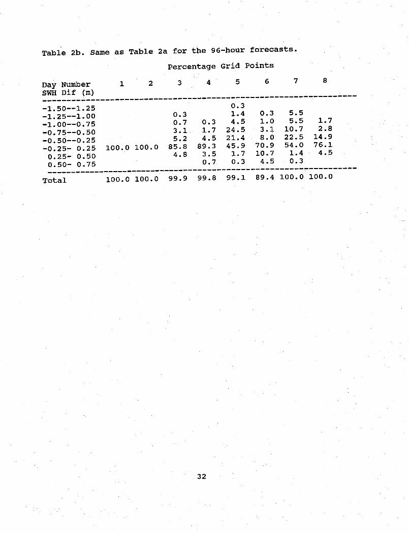
Table 2b. Same as Table 2a for the 96-hour forecasts.

Percentage Grid Points

Day Number 1 2 3 4 5 6 7 8

SWH Dif (m)

-1.50--1.25 0.3

-1.25--1.00 0.3 1.4 0.3 5.5

-1.00--0.75 0.7 0.3 4.5 1.0 5.5 1.7

-0.75--0.50 3.1 1.7 24.5 3.1 10.7 2.8

-0.50--0.25 5.2 4.5 21.4 8.0 22.5 14.9

-0.25- 0.25 100.0 100.0 85.8 89.3 45.9 70.9 54.0 76.1

0.25- 0.50 4.8 3.5 1.7 10.7 1.4 4.5

0.50- 0.75 0.7 0.3 4.5 0.3

Total 100.0 100.0 99.9 99.8 99.1 89.4 100.0 100.0

32

Table 3a. Distribution of SWH differences between the Janssen (JS)and the control run. Successive twelve-hour forecastsfor the northeast Pacific with 534 grid points. Thepercentage of grid points in the region with SWHdifference within the indicated interval are given.

Percentage Grid Points

Day Number 1 2 3 4 5 6 7 8 9

SWH Dif. (m)_________________________________________________________________

-0.75--0.50 0.4 0.7-0.50--0.25 0.6 0.7 0.2 1.5 1.9-0.25- 0.25 97.9 94.8 98.9 100.0 99.8 97.2 96.8 95.3 95.10.25- 0.50 1.5 4.5 1.1 0.2 1.9 3.0 2.4 1.90.50- 0.75 0.4 0.2 0.2

___Total 100.0 100.0 100.0 100.0 100.0 100._ 100.0 99.9 99.1_Total 100.0 100.0 100.0 100.0 100.0 100.1 100.0 99.9 99.1

33

Table 3b. Same as Table 3a for the 96-hour forecasts.

Percentage Grid Points

Day Number- .. !T T - ,

1 2 3 4 5 6 7 8 9

5WHi UlL. itml

-1.25--1.00 0.4

-1.00--0.75 0.4 0.2 0.2 0.2

-0.75--0.50 0.2 1.1 0.7 1.3 2.2

-0.50--0.25 0.7 0.9 2.1 6.7 0.2 4.7 4.7 8.0

-0.25- 0.25 85.4 95.1 92.0 91.6 81.7 92.0 84.7 84.5 85.8

0.25- 0.50 8.0 3.7 3.0 1.5 14.2 6.4 7.1 5.4 3.9

0.50- 0.75 4.5 0.2 1.5 0.2 4.1 1.4 1 7 2.4

0.75- 1.00 0.7 0.2 0.91.00- 1.25 0.3 0.6

Total 98.6 99.9 99.9 100.0 100.0 100.0 100.0 100.0 99.9

34

Table 4a. Same as Table 3a for the northwest Atlantic

Percentage Grid Points

Day Number 1 2 3 4 5 6 7 8 9

SWH Dif. (m)_________________________________________________________________-0.25-0.25 98.9 98.9 96.0 100.0 96.0 96.0 99.3 90.9 98.90.25- 0.50 1.1 1.1 4.0 3.6 4.0 0.7 9.1 1.1

_ _Total 100.0 100.0 100.0 100.0 99.6 100.0 100.0 100.0 100.0_Total 100.0 100.0 100.0 100.0 99.6 100.0 100.0 100.0 100.0

35

Table 4b. Same as Table 3b for the northwest Atlantic.

Perc

Day Number 1 2 3

SWH Dif. (m)

-1.00--0.75-0.75--0.50 0.3-0.50--0.25 2.4 1.0 0.3

-0.25- 0.25 94.1 94.1 92.40.25- 0.50 3.1 4.5 6.9

0.50- 0.75 0.3 0.30.75- 1.001.00- 1.251.25- 1.501.50- 1.751.75- 2.00

-entage Grid Points4 5 6

95.24.8

0.32.4 1.794.8 91.02.4 6.6

0.7

7 8 9

0.71.03.793.21.00.3

1.0 1.479.6 89.113.3 8.83.1 0.71.01.00.7

0.3

Total 99.9 99.9 99.9 100.0 99.9 100.0 99.9 99.7 100.0

--- -- -- -- -- -- -- -- -- -- .

36

FIGURE CAPTIONS.

Fig. 1. Wave growth parameter vs inverse wave age for differentvalues of the drag coefficient. Markers: Plant's data; solidlines: approximation from equations (2.7) and (2.8).

Fig. 2. Adaptation of Fig. 3 from Janssen (1989). Dimensionlesswind speed as a function of dimensionless height for u, = 0.7m/s. The thin line represents - ao.

Fig. 3. Reproduction of Fig. 7 from Janssen (1989). Aerodynamicdrag over sea waves as a function of wave age for twodifferent parameterizations of Phillips' constant.

Fig. 4. The coupling procedure. Downward arrows indicatetransfer of u, from the atmospheric model to the wave model,and upward arrows indicate transfer of zo from the global wavemodel to the atmosphere model. The "hindcast" continues forall the days of the experiment. Every 24 hours at 0000 UTC a120-hour wave forecast is initiated.

Fig. 5a. Contour plot of surface latent heat flux for the 24-hour forecast of the control run for 0000 UTC, January 8,1992.

Fig. 5b. Same as 5a for the JS run.

Fig. 6a. Contours of roughness height (z0) for the control runof January 8, 1992.

Fig. 6b. Same as Fig. 6a for the JS run.

Fig. 7a. Same as Fig. 5a for January 30, 1992.

Fig. 7b. Same as Fig. 5b for January 30, 1992, CS run.

Fig. 8. Contours of surface heat flux for the January 8, 1992control run.

Fig. 8b. Same as Fig. 8a for the JS run.

Fig. 9. Vector differences in the surface stresses between theCS and control runs for 0000 UTC January 30, 1992.

Fig. 10. Same as Fig. 9 for the 10-m height winds.

Fig. 11a. Contours of differences in SWH between the CS run andthe control run: coupled minus control. North Pacific forthe 12-hour forecast valid 1200 UTC January 30, 1992. Solidcontours indicate positive differences, dashed contoursindicate negative differences. Contour lines over land shouldbe disregarded.

37

Fig. l1b. Same as Fig. 11a for the north Atlantic.

Fig. 12a. Same as Fig. l1a for the 96-hour forecast valid

February 3, 1992.

Fig. 12b. Same as Fig. 11b for the 96-hour forecast valid

February, 2, 1992.

Fig. 13a. Forecast directional and frequency wave spectra at grid

point located at 45°N -130°W for the 96-hour forecast valid

0000 UTC February 3, 1992 for the control run. Arrow on the

margin of the directional spectrum indicates u*. Spectral

densities are normalized relative to the maximum spectral

density.

Fig. 13b. Same as Fig. 13a for the CS run.

38

1

10-1 x

'-, 10-2 00

V1

0 2

Figure 1i

10- 230 '~1

0

0

0

10-2 lo-' 1 10u./c

Figure 1.

39

.I-

P-.

A X

l

0o4::0

-1 1 10 100gz/u" -p-

3.5

CDX 10 3

3.0

2.5

2.0

1.55 10 15 20 25

Cp/U* -

Figure 3.

41

I.1

'10

: t Awl.t'3

VIbM'O Fc rr e Ce . - t

% I'.l kIWereIRo rerIfX Wea q ~e fr e, r & T

Wl AV C

I1

UUNIUUR INTERVRL= 100.00

8 JAN. OZ FT=MERN= -66.185

2L4 CON

150W 120W 90W 60W 30W OE 30E 60E 90ECONTOUR INTERVRL= 100.00

120E 150E 180MERN= -64.529

'1I-J-

titm

Alo

SFC LRTENT H FLX 1992

m0.

90S-180N

SFC LRTENT H FLX90N. i

1992 8 JRN. OZ FT= 24 JCL

tIj

I.

lid

(D

ROUGHNESS90N

n'

1. 992 8 .JRN. OZ FT= 0 WAVE MODELS

180WCONTOUR INTERVRL=1.OE-02 MERN= 0.007

H U U H 1 H 3 8 JAN. OZ FT= 0 HRVE MODELS

OE 90E 181CONTOUR INTERVRL=1.OE-02 MERN= 0.013

I-J

0%0~r

~1.

(I,

SFC LATENT H F'LX

-4

1992 30 JRN. OZ FT- 24 CON

-

t.

SFC LATENT H FLX 1992 30 JAN. OZFT= 214 CHR

9

E

MERN=

c0

I-J

0,

SF-C' HERT FLUX

3

A0

F -992 3 0 -- P- m 07 F-T - 24 CON9I

:P. tijI-'o

0"Qr

SFC HEAT FLUX 1992 30 JRN. OZ FT=L . . ; i i I I~~~~~~~~~~~~~~~~~~~~~~~~~~~~~~~~~~~~~~~~~~~~~~~~~~~~~~~~~~~~~~~~~~~~~~~~~~~~~~~~~~~~~~~~~~~~~~~~~~~~~~~~

uli0

24 CHR

Il-I

m0

ko

$STIRESS 1992 30 JAN. OZ FT= 214 CHRLIKOV.I V MINUS

9ON .3 .......... ~~~~~~~~~~~~~~~~~~~~~~~~~~~~~~~~~~~~~~~~~~~~~~~~~~~~~~~~~~~~~~~~~~~~~~~~~~~~~~~~~~~~~~~~~~~~~~~~~~~~~~~~~~~~~~~~~~~~~~~~~~~~~~~~~~~~~~~~~~~~.* 1~~~:;~~~:~~::::::::I:::. ~~~~~~~~~~~. .. :::.,:..I..~.......

EQ~~~~~~~~~~~~~~~~~~~~~~~~~~~~~~~~~~~~~~~ ..........~~~~~~~~~~~~~~~~~~~~~~~~~~~~~~~~~~~~~~~~~~~~~~~~~~ .I. ... I

... ... . . ...l:~~. .:........ :~.~ ........... ~~t:~::::::~~:I. .,,...

.....=. ~ ~ ~ ~ ~ ~ ~ ~ ~ ~ ~ ........

0 j" _7A..:~;.~::,,~..... ... ..... .. . ..... .

.. . .. . .. . .......... ....... 18......... ~~~ ~ UV ....... .L.. . 7RT R= 1E O2 M R: .180W 150W 1 20W 9UW bu

- 8.3 UNIT

nH)

I' U Wi ut- --- --- -- -FRCTOR= I.E+02 MEAN= 0.030

I

p-

Il.a(D

0$10 METER WIND 1992 30 JRN. OZ FT= 0 CHRLIKOV.IV MINUS.'''' .......................................... ........... ; ......... ;, i1N :::ii ,::ii:::,,.:: ..-i:::.,,, ---- t--............. :.i.: ......

... . .................... ;:::::::::: .W t ~ 5 - -s>-..;., - i....:... o.*~6se4 ...... --*l-.)_ .........>>.,a" ....... \at__14<,*-'st''L '.**............. ..................-

./ :.,,: ..... . .',.......

) N · .. ,.<, _Fs--w-.---48t ..~.. .:............!....... '- ~'-~,, *--:.:_..:.L:::~ .......................... *-.- -,-................... ,;.,,

14L~~~ . ......... ,'..·

~~~~,~.. .... .... .:l'~F-''s---'Y---n-"'-l-.b-'-f~t--.- ................. 1../¥.:................................................................;...... i. : : -6l---w t--\{#',- sslo --' ''--'-- * - * l/ ->g-'--' * ..... ,.............!_ ........~ ~ .. t ,....................... ~...................................................... ,'. : ..:::.::-:::'tl * ' '' /

.............. !,.,~' ,.t.... .... .... ", 4. : ...,...... .i.~i#-s^w -oz-- " tx;-''''- W..*o__s*.>X4..-' .. *w-e::;;.:;::v::^: ::: E'N ::, -...- I s''1tdy:; ^::t1 ~;';i d........ ':A ...........-,C .'_'...'. , ,.---m',4-^ ;ig ',' ..........' -' "! -%~- ............- ...... ....... *, ....

;0, ....... .t ' " ":"; ~ '~ '......... .I. .. .. .. ....

~~~~~~:::: '':......,,J... ..... ":::: :

JOS ~ ~~~~~~~~~~~~~~~~~~~~~~~~~~~~~~~~ ......... ........

J 3 .* .X. ..il.;-; 7;-- *; 4 ; / ;*)g>>-{}g ;*--- t Fl g -0;xC; ; ii yr ; ' i . . .. .. .. .. .. .. . . . . . .if ~~~~~~~~~~~~"..........,&i, x,. -"--' l .lS *-'" " M .:: ~iii! e 4^ ., ,-,, ,, *, . , .,, . ,,, ..,.,,,, .. , ., . ...................... .. .............

i05-~{~--~-~. ..... ....

180W 150W 120W 90W 60W 30W- 2.7 UNIT

OE 30E 60E 9U0E 1 lU I bUE IUUMERN= 0.010

60

'Nj

30

E

)C

90

r_

Figure lla.53

Figure l1b.54

SWH DIFF. [m] between coupled & control runs96h FCST VALID @ 2/ 3/92 0Z

-160.

-1.25 -1.00 -0.75 -0.50 -0.25 0.00 0.25 0.50 0.75 1.00CONTOUR FROH -1.7500 TO 1.2500 CONTOUR INTERVAL OF 0.25000 PT13.3)- 0.00000E00

Figure 12a.

55

60.

30.

0.-100.

SWH DIFF.[m) between coupled &

96h FCST VALID @ 2/ 3/92 0Z

-35.

control runs

20.

-1.25 -1.00 -0.75 -0.50 -0.25 0.00 0.25 0.50 0.75 1.00

CONTOUR FROM -1.7500 TO 1.2500 CONTOUR INTERVAL OF 0.25000 PTt3.3)= 0.09090E.00

Figure 12b.

56

60.

30.

9.

-9s.

.-

i

control runs

CONTROL RUN: DIRECTIONAL AND ONE DIMENSIONAL SPECTRA - 92020300

Frequency interval= 0.039 - 0.308. Directions from north(up)

LAT/LON= 45.0/-130.0. SWH= 8.3(m). U.STARt10= 7.501m/s). DIR= 20.9

19A I9, F { < f /

70

U,

e0

zw

Lii

50

40

30

29

10

0

FREQUENCY I[HzI

CONTOUR FROM 0.00008E.00 TO 100.00 CONTOUR INTERVAL OF 10.609 PTI3.3)- 0.00900E+00

Figure 13a.

57

I

COUPLED RUN: DIRECTIONAL AND ONE DIMENSIONAL SPECTRA - 92020300

Frequency interval= 0.039 - 0.308. Directions from north(up)

LAT/LON= 45.0/-130.0. SWH= 6.8(m). U.STAR*10= 6.40(m/s), OIR= 27.6

90

80

- 70

CIO

w60e

z

4048

LI30

L OF 10.009

Figure 13b.58

OPC Contributions (Cont.)

No. 19. Esteva, D.C., 1988: Evaluation of Priliminary Experiments Assimilating Seasat

Significant Wave Height into a Spectral Wave Model. Journal of Geophysical

Research. 93, 14,099-14,105

No. 20. Chao, Y.Y., 1988: Evaluation of Wave Forecast for the Gulf of Mexico. Proceedings

Fourth Conference Meteorology and Oceanography of the Coastal Zone, 42-49

No. 21. Breaker, L.C., 1989: E1 Nino and Related Variability in Sea-Surface Temperature

Along the Central California Coast. PACLIM Monograph of Climate Variability of the

Eastern North Pacific and Western North America. Geophysical Monograph 55. AGU, 133-

140.

No. 22. Yu, T.W., D.C. Esteva, and R.L. Teboulle, 1991: A Feasibility Study on Operational

Use of Geosat Wind and Wave Data at the National Meteorological Center. Technical

Note/NMC Office Note No. 380, 28pp.

No. 23. Burroughs, L. D., 1989: Open Ocean Fog and Visibility Forecasting Guidance System.

Technical Note/NMC Office Note No. 348, 18pp.

No. 24. Gerald, V. M., 1987: Synoptic Surface Marine Data Monitoring. Technical Note/NMC

Office Note No. 335, 10pp.

No. 25. Breaker, L. C., 1989: Estimating and Removing Sensor Induced Correlation form AVHRR

Data. Journal of Geophysical Reseach. 95, 9701-9711.

No. 26. Chen, H. S., 1990: Infinite Elements for Water Wave Radiation and Scattering.

International Journal for Numerical Methods in Fluids. 11, 555-569.

No. 27. Gemmill, W.H., T.W. Yu, and D.M. Feit, 1988: A Statistical Comparison of Methods for

Determining Ocean Surface Winds. Journal of Weather and Forecasting. 3, 153-160.

No. 28. Rao. D. B., 1989: A Review of the Program of the Ocean Products Center. Weather and

Forecasting. 4, 427-443.

No. 29. Chen, H. S., 1989: Infinite Elements for Combined Diffration and Refraction

Conference Preprint. Seventh International Conference on Finite Element Methods Flow

Problems. Huntsville. Alabama, 6pp.

N0. 30. Chao, Y. Y., 1989: An Operational Spectral Wave Forecasting Model for the Gulf of

Mexico. Proceedings of 2nd International Workshop on Wave Forecasting and

Hindcasting, 240-247.

No. 31. Esteva, D. C., 1989: Improving Global Wave Forecasting Incorporating Altimeter Data.

Proceedings of 2nd International Workshop on Wave Hindcasting and Forecasting,

Vancouver. B.C.. April 25-28. 1989, 378-384.

No. 32. Richardson, W. S., J. M. Nault, D. M. Feit, 1989: Computer-Worded Marine Forecasts.PreDrint. 6th Symp. on Coastal Ocean Management Coastal Zone 89, 4075-4084.

No. 33. Chao, Y. Y., T. L. Bertucci, 1989: A Columbia River Entrance Wave Forecasting

Program Developed at the Ocean Products Center. Techical Note/NMC Office Note 361.

No. 34. Burroughs, L. D., 1989: Forecasting Open Ocean Fog and Visibility. Preprint. 11th

Conference on Probabilitv and Statisitcs. Monterey. Ca., 5pp.

No. 35. Rao, D. B., 1990: Local and Regional Scale Wave Models. Proceeding (CMM/WMO)

Technical Conference on Waves, WMO. Marine Meteorological of Related Oceanographic

Activities Report No. 12, 125-138.

OPC CONTRIBUTIONS (Cont.)

No. 36. Burroughs, L.D., 1991: Forecast Guidance for Santa Ana conditions. Technical

Procedures Bulletin No. 391, llpp.

No. 37. Burroughs, L. D., 1989: Ocean Products Center Products Review Summary. Technical

Note/NMC Office Note No. 359. 29pp.

No. 38. Feit, D. M., 1989: Compendium of Marine Meteorological and Oceanographic Products

of the Ocean Products Center (revision 1). NOAA Technical Memo NWS/NMC 68.

No. 39. Esteva, D. C., Y. Y. Chao, 1991: The NOAA Ocean Wave Model Hindcast for LEWEX.

Directional Ocean Wave Spectra, Johns Hopkins University Press, 163-166.

No. 40. Sanchez, B. V., D. B. Rao, S. D. Steenrod, 1987: Tidal Estimation in the Atlantic

and Indian Oceans, 3° x 3° Solution. NASA Technical Memorandum 87812, 18pp.

No. 41. Crosby, D.S., L.C. Breaker, and W.H. Gemmill, 1990: A Difintion for Vector

Correlation and its Application to Marine Surface Winds. Technical Note/NMC Office

Note No. 365, 52pp.

No. 42. Feit, D.M., and W.S. Richardson, 1990: Expert System for Quality Control and Marine

Forecasting Guidance. Preprint. 3rd Workshop Operational and Metoerological. CMOS,

6pp.

No. 43. Gerald, V.M., 1990: OPC Unified Marine Database Verification System. Technical

Note/NMC Office Note No. 368, 14pp.

No. 44. Wohl, G.M., 1990: Sea Ice Edge Forecast Verification System. National Weather

Association Digest, (submitted)

No. 45. Feit, D.M., and J.A. Alpert, 1990: An Operational Marine Fog Prediction Model. NMC

Office Note No. 371, 18pp.

No. 46. Yu, T. W. , and R. L. Teboulle, 1991: Recent Assimilation and Forecast Experiments

at the National Meteorological Center Using SEASAT-A Scatterometer Winds. Technical

Note/NMC Office Note No. 383, 45pp.

No. 47. Chao, Y.Y., 1990: On the Specification of Wind Speed Near the Sea Surface. Marine

Forecaster Training Manual, (submitted)

No. 48. Breaker, L.C., L.D. Burroughs, T.B. Stanley, and W.B. Campbell, 1992: Estimating

Surface Currents in the Slope Water Region Between 37 and 410N Using Satellite

Feature Tracking. Technical Note, 47pp.

No. 49. Chao, Y.Y., 1990: The Gulf of Mexico Spectral Wave Forecast Model and Products.

Technical Procedures Bulletin No. 381, 3pp.

No. 50. Chen, H.S., 1990: Wave Calculation Using WAM Model and NMC Wind. Preprint. 8th ASCE

Engineering Mechanical Conference. 1, 368-372.

No. 51. Chao, Y.Y., 1990: On the Transformation of Wave Spectra by Current and Bathymetry.

Preprint. 8th ASCE Engineering Mechnical Conference. 1, 333-337.

No. 52. Breaker, L.C., W.H. Gemmill, and D.S. Crosby, 1990: A Vector Correlation

Coefficient in Geophysical: Theoretical Background and Application. Deed Sea

Research, (to be submitted)

No. 53. Rao, D.B., 1991: Dynamical and Statistical Prediction of Marine Guidance Products.

Proceedings. IEEE Conference Oceans 91, 3, 1177-1180.

OPC CONTRIBUTIONS (Cont.)

No. 54. Gemmill, W.H., 1991: High-Resolution Regional Ocean Surface Wind Fields.

Proceedings. AMS 9th Conference on Numerical Weather Prediction, Denver, CO, Oct.

14-18, 1991, 190-191.

No. 55. Yu, T.W., and D. Deaven, 1991: Use of SSM/I Wind Speed Data in NMC's GDAS.

Proceedings. AMS 9th Conference on Numerical Weather Prediction, Denver, CO, Oct.

14-18, 1991, 416-417.

No. 56. Burroughs, L.D., and J.A. Alpert, 1992: Numerical Fog and Visiability Guidance in

Coastal Regions. Technical Procedures Bulletin. (to be submitted)

No. 57. Chen, H.S., 1992: Taylor-Gelerkin Method for Wind Wave Propagation. ASCE 9th Conf.

Eng. Mech. (in press)

No. 58. Breaker, L.C., and W.H. Gemmill, and D.S. Crosby, 1992: A Technique for Vector

Correlation and its Application to Marine Surface Winds. AMS 12th Conference on

Probability and Statistics in the Atmospheric Sciences, Toronto, Ontario, Canada,

June 22-26, 1992.

No. 59. Breaker, L.C., and X.-H. Yan, 1992: Surface Circulation Estimation Using Image

Processing and Computer Vision Methods Applied to Sequential Satellite Imagery.

Proceeding of the 1st Thematic Conference on Remote Sensing for Marine Coastal

Environment, New Orleans, LA, June 15-17, 1992.

No. 60. Wohl, G., 1992: Operational Demonstration of ERS-1 SAR Imagery at the Joint Ice

Center. Proceeding of the MTS 92 - Global Ocean Partnership, Washington, DC, Oct.

19-21, 1992.

No. 61. Waters, M.P., Caruso, W.H. Gemmill, W.S. Richardson, and W.G. Pichel, 1992: An

Interactive Information and Processing System for the Real-Time Quality Control of

Marine Meteorological Oceanographic Data. Pre-print 9th International Conference

on Interactive Information and Processing System for Meteorology. Oceanography and

Hydrology, Anaheim, CA, Jan 17-22, 1993.

No. 62. Breaker, L.C., and V. Krasnopolsky, 1992: The Problem of AVHRR Image Navigation

Revisited. Intr. Journal of Remote Sensing (in press).

No. 63. Breaker, L.C., D.S. Crosby, and W.H. Gemmill, 1992: The Application of a New

Definition for Vector Correlation to Problems in Oceanography and Meteorology.

Journal of Atmospheric and Oceanic Technologv (submitted).

No. 64. Grumbine, R., 1992: The Thermodynamic Predictability of Sea Ice. Journal of

Glaciology, (in press).

No. 65. Chen, H.S., 1993: Global Wave Prediction Using the WAM Model and NMC Winds. 1993

International Conference on Hvdro Science and Engineering, Washington, DC, June 7 -

11, 1993. (submitted)

No. 66. Krasnopolsky, V., and L.C. Breaker, 1993: Multi-Lag Predictions for Time Series

Generated by a Complex Physical System using a Neural Network Approach. Journal of

Physics A: Mathematical and General, (submitted).

No. 67. Breaker, L.C., and Alan Bratkovich, 1993: Coastal-Ocean Processes and their

Influence on the Oil Spilled off San Francisco by the M/V Puerto Rican. Marine

Environmental Research, (submitted)

OPC CONTRIBUTIONS (Cont.)

No. 68. Breaker, L.C., L.D. Burroughs, J.F. Culp, N.L. Gunasso, R. Teboulle, and C.R. Wong,

1993: Surface and Near-Surface Marine Observations During Hurricane Andrew.

Weather and Forecasting, (in press).

No. 69. Burroughs, L.C., and R. Nichols, 1993: The National Marine Verification Program,

Technical Note, (in press).

No. 70. Gemmill, W.H., and R. Teboulle, 1993: The Operational Use of SSM/I Wind Speed Data

over Oceans. Pre-print 13th Conference on Weather Analyses and Forecasting,

(submitted).

No. 71. Yu, T.-W., J.C. Derber, and R.N. Hoffman, 1993: Use of ERS-1 Scatterometer

Backscattered Measurements in Atmospheric Analyses. Pre-print 13th Conference on

Weather Analyses and Forecasting, (submitted).

No. 72. Chalikov, D. and Y. Liberman, 1993: Director Modeling of Nonlinear Waves Dynamics.

J. Physical, (submitted).

No. 73. Woiceshyn, P., T.W. Yu, W.H. Gemmill, 1993: Use of ERS-1 Scatterometer Data to

Derive Ocean Surface Winds at NMC. Pre-print 13th Conference on Weather Analyses

and Forecasting, (submitted).

No. 74. Grumbine, R.W., 1993: Sea Ice Prediction Physics. Technical Note, (in press)

No. 75. Chalikov, D., 1993: The Parameterization of the Wave Boundary Layer. Journal of

Physical Oceanography, (to be submitted).

No. 76. Tolman, H., 1993: Modeling Bottom Friction in Wind-Wave Models. Waves 93 in New

Orleans, LA, (in press).

No. 77. Breaker, L., W. Broenkow, 1993: The Circulation of Monterey Bay and Related

Processes. Revised and resubmitted to Oceanography and Marine Biology: An Annual

Review, (to be submitted).

No. 78. Chalikov, D., D. Esteva, M. Iredell and P. Long, 1993: Dynamic Coupling between the

NMC Global Atmosphere and Spectral Wave Models. Technical Note, (to be submitted).

~k,AT OF co~

A:T Of ~tGTES of F