National Life Cycle Carbon Footprint Study for Production of US Swine

i

Final project report prepared by:

Greg Thoma, Ralph E. Martin Department of Chemical Engineering, University of Arkansas, Fayetteville, AR; gthoma@uark.edu

Darin Nutter, Department of Mechanical Engineering, University of Arkansas, Fayetteville, AR; dnutter@uark.edu

Richard Ulrich, Ralph E. Martin Department of Chemical Engineering, University of Arkansas, Fayetteville, AR; rulrich@uark.edu

Charles Maxwell, Department of Animal Sciences, University of Arkansas, Fayetteville, AR; cmaxwell@uark.edu

Jason Frank, DiamondV, Inc., Cedar Rapids, IA, jfrank@diamondv.com

Cashion East, The Sustainability Consortium, University of Arkansas, Fayetteville, AR; ceast@walton.uark.edu

May 15, 2011

ii

Table of Contents

2.1 Goal and Scope Definition ...............................................................................................................................5

2.1.1 Goal .........................................................................................................................................................5 2.1.2 Functional Unit .......................................................................................................................................5 2.1.3 Project Scope and System Boundaries ...................................................................................................5 2.1.4 Allocation ................................................................................................................................................5 2.1.5 Cut-off criteria ........................................................................................................................................6 2.1.6 Life cycle impact assessment ..................................................................................................................7 2.1.7 Audience .................................................................................................................................................7

2.2 Conceptual farm production model ................................................................................................................7

2.3 Life cycle inventories .......................................................................................................................................8

2.3.1 Crop production ......................................................................................................................................9 2.3.2 On-farm manure management ............................................................................................................ 11 2.3.3 Biogenic carbon ................................................................................................................................... 15 2.3.4 Farm to Processor Transportation ....................................................................................................... 16

2.4 Pork Processing and Packaging .................................................................................................................... 16

2.4.1 Methodology ....................................................................................................................................... 17 2.4.2 Uncertainty .......................................................................................................................................... 17 2.4.3 Electricity ............................................................................................................................................. 18 2.4.4 Fuel Energy .......................................................................................................................................... 18 2.4.5 Packaging Materials ............................................................................................................................. 18

2.5 Retail ............................................................................................................................................................ 18

2.5.1 Refrigerated Space Burden .................................................................................................................. 19 2.6 Consumer ..................................................................................................................................................... 19

2.6.1 Post-Consumer Solid Waste ................................................................................................................ 20 2.7 Software, Database and Model Validation ................................................................................................... 20

3.1 Life Cycle Phases........................................................................................................................................... 21

3.2 Overall Cradle-to-Grave GHG emissions. ..................................................................................................... 22

3.3 Scenario Analysis: ......................................................................................................................................... 24

3.3.1 Animal Rations ..................................................................................................................................... 24 3.3.2 Regional Analysis ................................................................................................................................. 26

3.4 Post farm supply chain ................................................................................................................................. 29

3.4.1 Meat Processing .................................................................................................................................. 30 3.5 Retail Supermarkets ..................................................................................................................................... 31

4.1.1 Scenario and Sensitivity Analysis ......................................................................................................... 34

Executive Summary ......................................................................................................................... 1

1 Introduction .............................................................................................................................. 3

2 LCA Methodology ...................................................................................................................... 3

3 Scan level carbon footprint results ......................................................................................... 20

4 Discussion and Interpretation ................................................................................................. 33

iii

4.2 Data Quality, Uncertainty and Reconciliation .............................................................................................. 36

4.2.1 Uncertainty in Input Variables ............................................................................................................. 36 4.2.2 Monte Carlo Simulation ....................................................................................................................... 36 4.2.3 Assigning Distributions to Variables .................................................................................................... 37 4.2.4 Data Quality Assessment ..................................................................................................................... 38 4.2.5 Consistency assessment ...................................................................................................................... 38

4.3 Model Validation .......................................................................................................................................... 40

First Round Critical Review Life Cycle Greenhouse Gas Emissions Baseline Study for the U.S. Pork Industry ..... 48

Second Round Critical Review Life Cycle Greenhouse Gas Emissions Baseline Study for the U.S. Pork Industry 64

5 Conclusions ............................................................................................................................. 41

6 Literature Cited ....................................................................................................................... 42

Appendix A Comparison with other protein sources ................................................................... 45

Appendix B. Model parameters used for sensitivity and scenario analysis ................................ 46

Appendix C Third party critical review .......................................................................................... 48

iv

List of Tables Table 1. Typical Sow Diet – Without DDGs ................................................................................... 11

Table 2. Typical Sow Diet – With DDGs ......................................................................................... 11

Table 3. Nursery and Grow-Finish Typical Diet – Without Distillers Grains ................................. 12

Table 4. Nursery and Grow-Finish Typical Diet – With Distillers Grains ....................................... 12

Table 5. Production regions used in national scale analysis and weighted fraction of animals with specific manure management practices. .............................................. 13

Table 6. Average manure characteristics as predicted by ASABE equations. ............................. 13

Table 7. Economic census data used for allocation in processing and packaging ....................... 17

Table 8 Unit Process Names and Descriptions for Network Diagrams ......................................... 22

Table 9. Cradle to farm gate sensitivity parameters. Each row has parameters for a simulation. Shaded cells were the only parameter changed during each run (defined by a row). ...................................................................................................... 29

Table 10. Parameters evaluated in post-farm gate scenario testing........................................... 30

Table 11. Summary of EU pork production GWP data: Functional unit = 1kg carcass at farm gate. .................................................................................................................... 33

Table 12. Parameter ranges for manure management systems sensitivity analysis ................... 35

Table A 1. Reported GHG emissions associated with alternative animal protein sources. ........ 45

Table B 2. Input parameters used for the base case scenario ..................................................... 46

Table B 3. Calculated parameters ................................................................................................ 47

v

List of Figures Figure 1. Relative contribution from different phases of the supply chain to the

cumulative GHG emissions. .......................................................................................... 2

Figure 2. Stages of a life cycle assessment .................................................................................... 4

Figure 3. Schematic of pork production supply chain showing major inputs and outputs relevant to greenhouse gas emissions. Boxes with white fill are not included within the system boundary. ........................................................................................ 6

Figure 4. Schematic of simplified pork production. Material and energy flows are integrated over the productive life of a single sow. The farm gate cumulative consumption of feed and energy required to finish all the litters produced by one sow is allocated to the total finished weight of her litters. ................................... 8

Figure 5. Information diagram for calculating GHG emissions per amount of feed crop produced. ...................................................................................................................... 9

Figure 6. Distribution of hogs in the U.S. ..................................................................................... 14

Figure 7. Network diagram key. .................................................................................................... 21

Figure 8. Cumulative GHG emissions associated with consumption of pork in the US. The legend entries are discussed in the text. The estimates in this analysis do not include GHG emissions from pork destined for overseas consumption or food service industry emissions. ......................................................................................... 23

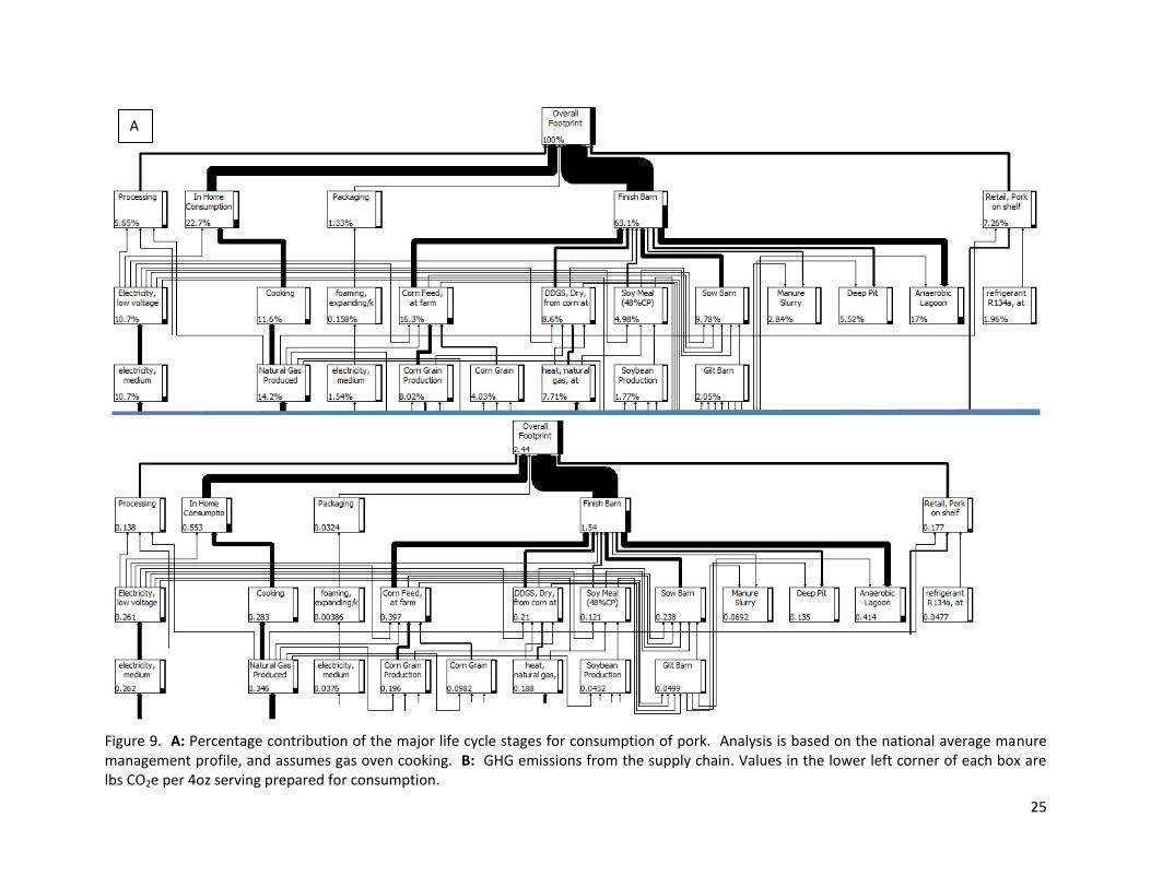
Figure 9. A: Percentage contribution of the major life cycle stages for consumption of pork. Analysis is based on the national average manure management profile, and assumes gas oven cooking. B: GHG emissions from the supply chain. Values in the lower left corner of each box are lbs CO2e per 4oz serving prepared for consumption. ......................................................................................... 25

Figure 10 Comparison of lifecycle emissions with or without DDGs included in the ration. The rations were modeled to provide necessary energy and protein content. Most categories are similar except for energy consumption, which is larger when DDGs are included in the diet. .......................................................................... 26

Figure 11. Cumulative metric tons of CO2e associated with pork production in the U.S. These estimates are based on federally inspected units reported for the regions shown in the legend. The total boneless weight estimated from these data correlate very closely to the per capita pork consumption reported by the Economic Research Service (47 lb/person/year). This analysis does not account for the structure of the industry where sow operations are not necessarily near the nursery finish operations. For purposes of this analysis, the sow operation footprint was estimated as coming from the same region as the finished animals. The region and production weighted national average carbon

vi

footprint is 2.87 lb CO2e per lb live weight at the farm gate (equivalent to 3.83 lb/lb dressed carcass or 5.9 lb CO2e/lb boneless meat). ............................................ 27

Figure 12. Comparison of manure management system choice on farm-gate cumulative GHG emissions. Note that the bar for piglets is different between the scenarios because of differences in manure management at the sow barn. The same manure management was selected for both the nursery-finish and sow barns. These scenarios all include DDGs in the ration. The vertical gray bars represent the 95% confidence interval based on 1500 Monte Carlo runs. ............... 28

Figure 13. Sensitivity analysis for farm gate production. Reported on a boneless meat basis ............................................................................................................................ 30

Figure 14. Post farm-gate sensitivity analysis. The most significant change is associated with the difference between gas and electric oven for cooking the meat. The last column is based on the assumption that retail and consumer phase allocation to pork follows the space occupied fraction of refrigerated and total store space for refrigeration burden (retail and consumer) and store overhead / consumer transport. ................................................................................................. 31

Figure 15. Gate-to-Gate impact of pork processing. The contribution is driven almost exclusively by natural gas and electricity. The overall footprint also includes diesel, gasoline, and fuel oil consumption as well as methane released from wastewater treatment facilities. The carbon dioxide in the third box represents the production burden from liquid carbon dioxide or dry ice. The difference

(~0.021 lb CO2e) between the sum of the 5 input boxes and the reported value

for the dressed carcass leaving is the direct emissions of the purchased carbon dioxide or dry ice. Note that this diagram reference flow for processing is 4oz of meat prepared for consumption. The diesel consumption for this phase includes all transport of live animals from the farm gate to the processing facility. ......................................................................................................................... 32

Figure 16. Comparison of regional differences and the effects of uncertainty in emission factors for manure management systems. Region 4 has a larger fraction of anaerobic lagoons than reported for regions 5 or 7, and thus has a markedly lager GHG emissions profile. ....................................................................................... 37

Figure 17. Database contribution to the carbon footprint for different supply stages. The green bar represents information collected or explicitly calculated for this project and includes, for example, emissions arising from crop residue. The red bar represents the contribution from economic input output data. ......................... 39

1

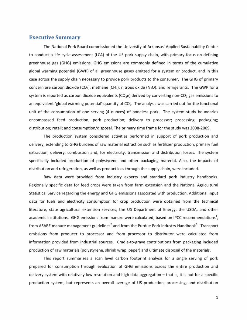
Executive Summary

The National Pork Board commissioned the University of Arkansas’ Applied Sustainability Center

to conduct a life cycle assessment (LCA) of the US pork supply chain, with primary focus on defining

greenhouse gas (GHG) emissions. GHG emissions are commonly defined in terms of the cumulative

global warming potential (GWP) of all greenhouse gases emitted for a system or product, and in this

case across the supply chain necessary to provide pork products to the consumer. The GHG of primary

concern are carbon dioxide (CO2); methane (CH4); nitrous oxide (N2O); and refrigerants. The GWP for a

system is reported as carbon dioxide equivalents (CO2e) derived by converting non-CO2 gas emissions to

an equivalent ‘global warming potential’ quantity of CO2. The analysis was carried out for the functional

unit of the consumption of one serving (4 ounces) of boneless pork. The system study boundaries

encompassed feed production; pork production; delivery to processor; processing; packaging;

distribution; retail; and consumption/disposal. The primary time frame for the study was 2008-2009.

The production system considered activities performed in support of pork production and

delivery, extending to GHG burdens of raw material extraction such as fertilizer production, primary fuel

extraction, delivery, combustion and, for electricity, transmission and distribution losses. The system

specifically included production of polystyrene and other packaging material. Also, the impacts of

distribution and refrigeration, as well as product loss through the supply chain, were included.

Raw data were provided from industry experts and standard pork industry handbooks.

Regionally specific data for feed crops were taken from farm extension and the National Agricultural

Statistical Service regarding the energy and GHG emissions associated with production. Additional input

data for fuels and electricity consumption for crop production were obtained from the technical

literature, state agricultural extension services, the US Department of Energy, the USDA, and other

academic institutions. GHG emissions from manure were calculated, based on IPCC recommendations1,

from ASABE manure management guidelines2 and from the Purdue Pork Industry Handbook3. Transport

emissions from producer to processor and from processor to distributor were calculated from

information provided from industrial sources. Cradle-to-grave contributions from packaging included

production of raw materials (polystyrene, shrink wrap, paper) and ultimate disposal of the materials.

This report summarizes a scan level carbon footprint analysis for a single serving of pork

prepared for consumption through evaluation of GHG emissions across the entire production and

delivery system with relatively low resolution and high data aggregation – that is, it is not for a specific

production system, but represents an overall average of US production, processing, and distribution

2

systems. The available life cycle data, by production stage, and the methodology for calculation of the

carbon footprint are described. It was found that the major impacts of pork production occur in crop

production, manure management, retail distribution and consumption. The overall estimate of the

carbon footprint for preparation and consumption of one 4 ounce serving was found to be 2.48 lb CO2e

with a 95% confidence band from 2.2 lb CO2e to 2.9 lb CO2e. Please note that the metric system was

used for all our calculations and the final results were converted to English units for presentation.

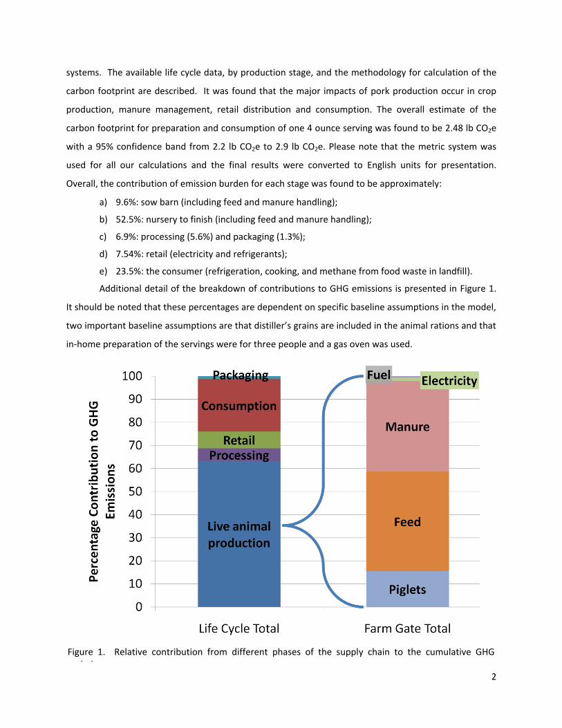
Overall, the contribution of emission burden for each stage was found to be approximately:

a) 9.6%: sow barn (including feed and manure handling);

b) 52.5%: nursery to finish (including feed and manure handling);

c) 6.9%: processing (5.6%) and packaging (1.3%);

d) 7.54%: retail (electricity and refrigerants);

e) 23.5%: the consumer (refrigeration, cooking, and methane from food waste in landfill).

Additional detail of the breakdown of contributions to GHG emissions is presented in Figure 1.

It should be noted that these percentages are dependent on specific baseline assumptions in the model,

two important baseline assumptions are that distiller’s grains are included in the animal rations and that

in-home preparation of the servings were for three people and a gas oven was used.

Figure 1. Relative contribution from different phases of the supply chain to the cumulative GHG emissions.

3

1 Introduction

The National Pork Board commissioned the University of Arkansas’ Applied Sustainability Center

to perform a life cycle assessment (LCA) of the pork supply chain which focused on defining greenhouse

gas (GHG) emissions. The pork supply chain is broadly divided into 8 stages; each receiving separate

analyses that were combined to provide the entire life cycle footprint. These stages are: feed

production; live animal production; delivery to processor; processing; packaging; distribution; retail; and

consumption/disposal.

Analysis of the pork supply chain can be used to provide the insight necessary to identify critical

leverage points where, in turn, innovation can lead to increased efficiency in the supply chain while

simultaneously leading to reductions in the carbon footprint of pork products. This project has been

conducted in compliance with ISO 14040:2006 and 14044:2006 standards for life cycle assessment. It

should be noted that a full LCA should also evaluate impact metrics that include other effects such as

human health impact, ecosystem quality, and resource depletion. Because the intent of the study was

to have the results reported to third parties, this project has received a post-hoc review by an external

panel of experts led by Dr. Robert Anex, University of Wisconsin, Dr. Pascal Lesage, Interuniversity

Research Center for the Life cycle of Products, Processes and Services (CIRAIG), École Polytechnique de

Montréal, and Dr. Doug Reinemann, University of Wisconsin. The review panel had full access to the

SimaPro model for their review. The review comments and authors’ responses are presented as

Appendix B following the body of the report.

2 LCA Methodology

LCA is a tool to evaluate environmental impacts of a product or process throughout the entire

life cycle, which for agricultural products begins with production of fertilizers, and then crop cultivation,

and animal husbandry, through processing, use and disposal of wastes associated with its final end-use.

This includes identifying and quantifying energy and materials used and wastes released to the

environment, calculating their environmental impact, interpreting results, and evaluating improvement

opportunities.

This LCA has been structured following ISO 14040:2006, and ISO 14044:2006 standards which

provide an internationally agreed method of conducting LCA, but leave significant degrees of flexibility

in methodology to customize individual projects to their desired application and outcomes.

Figure 1 depicts the core LCA steps and highlights the iterative nature of the process. The goal

and scope definition phase is a planning process, which involves defining and describing the product,

4

process or activity; establishing the aims and context in which the LCA is to be performed; and

identifying the life cycle stages and environmental impact categories to be reviewed for the assessment.

The depth and breadth of LCA can differ considerably depending on the goal of the LCA.

The life cycle inventory analysis phase (LCI phase is the second phase of LCA) is an inventory of

input/output material and energy flows with regard to the system being studied; it involves identifying

and quantifying energy, water, materials and environmental releases (e.g.: air emissions, solid wastes,

wastewater discharge) during each stage of the life cycle.

The life cycle impact assessment phase (LCIA) is the third phase of the LCA. This step calculates

human and ecological effects of material consumption and environmental releases identified during the

inventory analysis. For this study, the Global Warming Potential (GWP) was analyzed and reported.

GWP is an important effect related to climate change and is one of several common LCIA impact

categories. Others include eutrophication, acidification, ozone depletion, land use, etc. Readers should

be cautioned that interdependencies may exist between impact categories and poor decisions can be

made when only a single impact metric is used as the basis.

Life cycle interpretation is the final phase of the LCA procedure, in which the results are

summarized and discussed. Its goal is to identify the most significant environmental impacts and the

associated life cycle stage, and highlight opportunities for potential change or innovation.

Figure 2. Stages of a life cycle assessment

5

2.1 Goal and Scope Definition

2.1.1 Goal

Determine GHG emissions associated with delivery, preparation, and consumption of one

serving of pork to US consumer. Because of the strong link between energy consumption and

greenhouse gas emissions, it is frequently the case that high greenhouse gas emissions are indicative of

opportunities for improved energy efficiencies or conservation. In addition, this analysis will provide an

understanding of the industry’s baseline level of greenhouse gas emissions which will be beneficial if

voluntary carbon trading markets become viable in the future.

2.1.2 Functional Unit

The functional unit of this study was one 4 ounce (uncooked weight) serving of boneless pork

prepared for consumption by a US consumer. We do not differentiate among cuts of meat in this

analysis.

2.1.3 Project Scope and System Boundaries

This life cycle assessment was a cradle-to-grave analysis of the carbon footprint or global

warming potential of the production and consumption of boneless pork. The system boundaries, shown

schematically in Figure 3 (including the gray boxes), encompassed effects beginning with GHG emissions

associated with raw material extraction from nature through greenhouse gas emissions from either

landfill or municipal waste incineration of the packaging. Incidental effects such as employee’s

commutes, nor the cost of heating the farmer’s residence have not been included. In addition, we have

not specifically accounted for long-term storage of carbon in non-consumed parts of the animal

specifically leather and meet which may not decompose in a landfill. Nor does the scope of this project

extend to other potential environmental effects such as nutrient runoff, topsoil loss, or depletion of

freshwater supplies; it focused on evaluation, at the national scale, of the global warming potential

attributable to production and consumption of pork in the United States. The primary time frame for

the study is 2008 - 2009.

2.1.4 Allocation

Where co-products are produced, an allocation of burdens associated with the unit process is

necessary. We evaluated allocation choices by the ISO hierarchy for allocation. There are three stages in

the supply chain where allocation occurs: first for byproducts of feed processing (e.g., distiller’s grains

and soy meal); second at the processing gate where allocation between dressed carcass and rendering

6

products occurs, and finally at retail and consumption where an allocation of refrigeration burdens and

a fraction of consumer transport of groceries is necessary.

The ISO approach recommends system separation as highest priority. For the allocation

necessary in this project there exists a situation of joint production, where the relative quantities of, for

example meal and oil, cannot be independently varied (beyond variation in the oil content of the seeds)

which causes the allocation priority to be system expansion. As this is a scan type or streamlined LCA,

the analysis required to identify the substitute products and ensure that quality LCI data exist was

deemed out of the project scope, and we have adopted economic value allocation (lowest of ISO

hierarchy) as a base case approach and consider a mass allocation for feed byproducts for comparison.

Due to the proprietary nature of economic data at retail, we have used a shelf space and sales approach

to estimate an appropriate allocation of retail and in-home burdens.

2.1.5 Cut-off criteria

The cut-off criterion for the study, and generally applied at the scale of an individual stage of life

cycle, is as follows: if a flow contributes less than 1% of the cumulative global warming potential, it may

Figure 3. Schematic of pork production supply chain showing major inputs and outputs relevant to greenhouse gas emissions. Boxes with white fill are not included within the system boundary.

7

be omitted from the model; however, small flows are not omitted when data are readily available.

Specific processes that were excluded on this principle were insemination and other veterinary inputs;

employee commuting and incidental energy consumption associated with on-farm residences or offices

were also estimated to be deminimus contributions. We did not include accounting, legal or other

services for individual farms, processors or retail outlets. In addition to these exclusions, we did not

account for infrastructure.

2.1.6 Life cycle impact assessment

For this project, a single impact assessment metric was chosen, global warming potential (GWP).

We have adopted the most recent IPCC recommended 100 year time horizon GWP equivalents for this

project4: CO2 = 1; CH4 = 25; and N2O = 298. Global warming potential equivalents are also presented for

most common refrigerants in this document. Biogenic carbon and methane impacts are discussed in

§2.3.3.

2.1.7 Audience

Stakeholders in the pork industry value chain are the intended audience for this study. This

study is not intended for comparative purposes, but is intended for third parties, and as such has

undergone an external review, described above. The study has been undertaken primarily as a tool to

identify opportunities for increasing efficiency and to provide a baseline evaluation of the industry’s

contribution to the U.S. greenhouse gas emissions inventory. Consumers increasingly express an

interest in understanding of the environmental impacts of the products they purchase, and thus

consumers represent a second potential audience for the study results. The LCA supports the pork

industry’s ability to work proactively with retailers to educate consumers about agricultural and food

sustainability issues.

2.2 Conceptual farm production model

To simplify mass and energy accounting we have chosen not to use a barn or batch of weaned

piglets as the computational basis, instead the computational farm model is based on the productive life

of one sow. The average number of litters (parities) and the number of piglets per litter are used to

determine the total feed and on-farm energy requirements. The cumulative and GWP impacts from all

the inputs are divided by the total mass of the finished animals produced from that sow. A schematic is

shown in Figure 4.

8

Thus the farm-gate footprint is: ∑ ∑

( ) on a live weight basis;

the inputs in the equation include the replacement gilts. This result can be converted to a carcass or

boneless basis using the live-to-purpose conversion of: 0.75 lb carcass per lb live weight, and the

carcass-to-boneless conversion: 0.65 lb boneless meat per lb carcass.

2.3 Life cycle inventories

A previously conducted literature review is used as the basis for much of the life cycle inventory

data5, and additional discussions with industry representatives and other experts helped fill in the data

gaps. The production system encompassed activities performed in support of pork production and

delivery extending to GHG burdens of raw material extraction for fertilizer production, primary fuel

extraction, delivery, combustion and, for electricity, transmission and distribution losses. The system

included production of polystyrene foam shells, shrink wrap, and adsorbent pads used to package meats

in supermarkets. We also included the impacts of distribution and refrigeration. The life cycle calculation

approach adopted for this work was largely process based; we used Economic Input-Output data for

whey in the animal ration because suitable process based datasets were not readily available. This was

to avoid errors associated with exclusion of GHG emission burdens. The inclusion of EIO data does add

some uncertainty to the analysis because of differences in the underlying basis for EIO estimates of

impact contributions. In particular, EIO System boundaries are more extensive than boundaries for

Figure 4. Schematic of simplified pork production. Material and energy flows are integrated over the productive life of a single sow. The farm gate cumulative consumption of feed and energy required to finish all the litters produced by one sow is allocated to the total finished weight of her litters.

9

process based analysis. We have included an analysis of the percentage of the total GHG emissions

arising from EIO datasets in §4.2.5. It should also be noted that some data are not from the US, in

particular much of the background data used in the study comes from the European based data in

EcoInvent and may not be completely representative of US conditions. These data include activities like

petroleum refining and some electricity generation technologies (e.g., wind and hydro) for which US

data do not exist. Foreground processes (those typically under direct control of the main supply chain

actors) are all linked to the US electricity grid mix; however, many background processes, taken without

modification from EcoInvent, remain linked to EU electricity mixes. In our judgment, any differences in

these background processes will not affect the study conclusions.

2.3.1 Crop production

In consultation with industry experts, we have identified the most common feeds6,7 and have

collected available information from farm extension and the National Agricultural Statistical Service

regarding the energy and greenhouse gas emissions associated with production of these crops.

2.3.1.1 Corn, DDGs, Soybean Meal

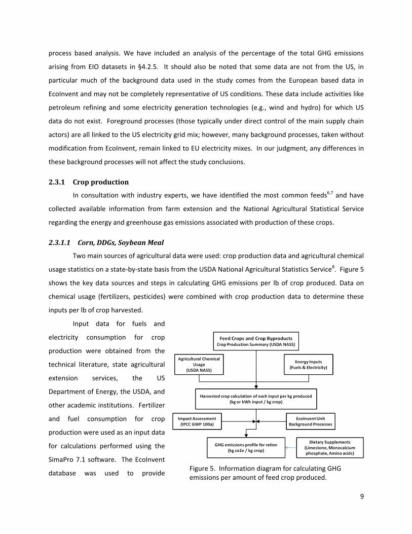
Two main sources of agricultural data were used: crop production data and agricultural chemical

usage statistics on a state-by-state basis from the USDA National Agricultural Statistics Service8. Figure 5

shows the key data sources and steps in calculating GHG emissions per lb of crop produced. Data on

chemical usage (fertilizers, pesticides) were combined with crop production data to determine these

inputs per lb of crop harvested.

Input data for fuels and

electricity consumption for crop

production were obtained from the

technical literature, state agricultural

extension services, the US

Department of Energy, the USDA, and

other academic institutions. Fertilizer

and fuel consumption for crop

production were used as an input data

for calculations performed using the

SimaPro 7.1 software. The EcoInvent

database was used to provide Figure 5. Information diagram for calculating GHG emissions per amount of feed crop produced.

10

upstream/background information (e.g., production of fertilizer, diesel, natural gas, etc) and the IPCC

GWP 100a impact assessment methodology was used to summarize the GWP of cradle-to-gate crop

production. Industry estimates were used to calculate the transportation burden associated with

moving the grains to feed mills which are typically near animal production facilities.

Distiller’s grain production was modeled using an EcoInvent unit process created for US

conditions. This unit process accounts for the fermentation, drying and other processes in a typical US

corn ethanol plant. The allocation between ethanol and DDGs is based on economic value of the

products, except that the energy for drying the distiller’s grains to facilitate longer distance transport is

allocated entirely to the DDGs. The allocation of other inputs is, including the corn grain, is 1.2%

allocated to distiller’s grains; this allocation fraction was reported on the EcoInvent website, and

adopted as the baseline economic allocation for this study. Information available from the Agricultural

Marketing Resource Center9, combined with an average production of 2.8 gallons of ethanol and 17.4

lbs of distillers grain per bushel of corn results in an average allocation of 18.5% to distiller’s grains.

Using this alternate economic allocation increases the footprint of the DDGs from 0.94 lb CO2e/lb DDGs

to 1.1 lb CO2e/lb DDGs.

We adapted the recent United Soybean Board LCA for the production of biodiesel from soy oil as

the basis for the soybean meal carbon footprint10. An economic allocation among soy oil, meal and hulls

was used. Economic allocation fractions were meal: 56.5%; oil: 41.6%; hulls: 1.9%, and mass allocation

fractions (for sensitivity analysis) were meal: 74.25%; oil: 19.34%; hulls: 6.41%.

2.3.1.2 CO2e emissions from lime, urea, pesticides, and fertilizer application

Nitrous oxide emissions attributed to crop production were taken to be 1% of applied nitrogen1.

No distinction between inorganic fertilizer and manure application was made in regard to direct nitrous

oxide release. However, the ammonia volatilization fraction for applied manure was taken as 20% rather

than 10%, leading to slightly larger indirect N2O emissions from manure N than inorganic N. For the

scale of the analysis conducted, there is not sufficient resolution in the underlying data regarding crop

rotation, tillage, and soil type to justify more complex estimation of the N2O emission. GWP burdens

associated with other fertilizers, including lime, and pesticides were accounted for in the inventory data

obtained from EcoInvent. Decomposition of crop residue contributes some N to the soil nitrogen cycle,

and results in additional N2O emission. The IPCC recommendations for estimation of crop residue

related emissions have been followed11.

11

2.3.1.3 Calculation of the cradle to mouth feed footprint.

Note that our initial analysis defined dry distiller grains (DDGs), a byproduct of corn ethanol

production, as an important contributor

to GWP of the feed. We have

performed an analysis using two diets:

one with and one without DDGs6,7.

Estimated feed consumption and

composition are given in Table 1 through

Table 4. Assuming 9.5 piglets per litter,

the total quantity of each feed

component consumed by all the animals

passing through the system over the

course of 3.5 litters (on average) for a

sow was calculated. In essence, this is

an integration of all of the feed crossing

the farm gate resulting in an average

production of 32.25 finished pigs plus

one sow. The total quantity of each feed

component was multiplied by the

carbon footprint for the production of that feed to give the overall feed footprint. Tables 1 and 2

present the information for a single lactation, and thus, on average, 3.5 times that amount of feed

would be accounted for in production of 32.25 finished pigs plus one sow. In Tables 3 and 4, the ration

being fed is keyed to the animal’s bodyweight (BW); all animals are assumed to reach a finish weight of

268 lb.

2.3.2 On-farm manure management

Different manure management systems result in different quantities of greenhouse gases,

primarily methane and nitrous oxide, emitted to the atmosphere. The IPCC provides guidance on

estimating the quantities of greenhouse gases which are emitted as a function of the specific

management system1. We have used the American Society of Agriculture Engineers (ASAE)12

recommendations to predict the quantity of manure generated, as well as to estimate the amount of

nitrogen excreted in the manure. Manure management systems included in the model are deep pit,

anaerobic lagoons, solid store, liquid slurry and pasture. Each can be modeled separately for scenario

Table 1. Typical Sow Diet – Without DDGs

Sow Feed

Breeding Gestation Lactation

Est. feed, lb/sow 50 600 252

% Corn 66.1 81.5 66.1

% DDGS 0.0 0.0 0.0

% SBM 27.0 14.5 27.0

%FAT 2.0 2.0 2.50

%Supplement 0.7 0.7 0.7

%Dical/limestone 2.9 2.9 3.0

Table 2. Typical Sow Diet – With DDGs

Sow Feed

Breeding Gestation Lactation

Est. feed, lb/sow 50 600 252

% Corn 58.0 53.0 58.0

% DDGS 10.0 30.0 10.0

% SBM 25.0 11.0 25.0

%FAT 2.0 2.0 2.35

%Supplement 0.7 0.7 0.8

%Dical/limestone 2.5 2.5 2.9

12

comparison as presented in §3.3.2 below. In addition, for national scale analysis, the fraction of manure

handled by each of the practices is accounted at a regional scale (See Table 5).

2.3.2.1 Methane and nitrous oxide emission due to manure management

We employed standardized methodologies as laid out in the IPCC 2006 guidelines in estimating

the annual CH4 and N2O emission factor (EFT) from manure1. We have used the ASABE guidelines to

define the average manure characteristics (Table 6), in particular the volatile solids content which is

significant in determining the quantity of methane that can be produced under anaerobic conditions.

Table 3. Nursery and Grow-Finish Typical Diet – Without Distillers Grains Pigs Nursery Grow-Finish

Phase I Phase II Phase III Grower I Grower II Finisher I Finisher II Finisher III

BW, lb 11-15 15-25 25-50 50-95 95-140 140-185 185-230 230-270

Gain, lb 4 10 25 45 45 45 45 40

Days in period 7 14 21 24 23 22 23 24

Est. feed, lb/pig 5 15 48 100 113 131 148 145

% Corn 37.9 51.9 59.2 62.8 68.5 74.3 80.9 83.9

% DDGs 0.0 0.0 0.0 0.0 0.0 0.0 0.0 0.0

% SBM 20.0 28.0 34.8 31.3 26.0 20.8 15.3 12.3

% Dried Whey 25.0 10.0 0.0 0.0 0.0 0.0 0.0 0.0

%Fat 5.0 3.0 1.5 2.5 2.5 2.5 1.5 1.5

%Supplement 3.3 3.1 2.0 1.1 1.1 1.0 0.9 0.9

%Dical/limestone 1.3 1.8 2.6 2.3 1.9 1.5 1.5 1.5

%bone/blood meal 7.5 2.3 0.0 0.0 0.0 0.0 0.0 0.0

Table 4. Nursery and Grow-Finish Typical Diet – With Distillers Grains

Pigs Nursery Grow-Finish

Phase I Phase II Phase III Grower I Grower II Finisher I Finisher II Finisher III

BW, lb 11-15 15-25 25-50 50-95 95-140 140-185 185-230 230-270

Gain, lb 4

10 25 45 45 45 45 40

Days in period 7 14 21 24 23 22 23 24

Est. feed, lb/pig 5 15 48 100 113 131 148 145

% Corn 33.8 43.9 47.2 50.7 56.3 62.1 68.6 83.9

% DDGS 5.0 10.0 15.0 15.0 15.0 15.0 15.0 0.0

% SBM 19.2 26.2 32.2 28.7 23.6 18.3 12.9 12.3

% Dried Whey 25.0 10.0 0.0 0.0 0.0 0.0 0.0 0.0

%Fat 5.0 2.9 1.4 2.3 2.3 2.4 1.4 1.5

%Supplement 2.0 2.2 1.9 1.1 1.1 1.0 0.9 0.9

%Dical/limestone 1.2 1.7 2.4 2.1 1.7 1.3 1.3 1.5

%bone/blood meal 7.5 2.3 0.0 0.0 0.0 0.0 0.0 0.0

13

The temperature is also an important parameter in the estimation of methane release associated with

each of the manure management techniques. U.S. monthly average temperature data were extracted

from the National Climatic Data Center. This temperature information was used in estimation of the

methane emissions from manure handling to account for the difference in mean temperature among

the 10 USDA production regions.

Other variables used in the model are the volatile solids (VST) of the manure and the maximum

methane production capability (B0 = 0.48 m3CH4/kg VS) (Table 10 A71)1:

( )

[∑

( )]

EF is the emissions in kilograms methane per animal per year and

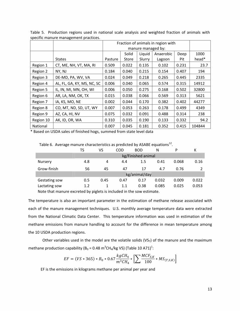
Table 5. Production regions used in national scale analysis and weighted fraction of animals with specific manure management practices.

Fraction of animals in region with manure managed by:

States Pasture

Solid Store

Liquid Slurry

Anaerobic Lagoon

Deep Pit

1000 head*

Region 1 CT, ME, NH, VT, MA, RI 0.509 0.022 0.135 0.102 0.231 23.7

Region 2 NY, NJ 0.184 0.040 0.215 0.154 0.407 194

Region 3 DE-MD, PA, WV, VA 0.024 0.049 0.218 0.265 0.445 2335

Region 4 AL, FL, GA, KY, MS, NC, SC 0.006 0.040 0.065 0.574 0.315 14912

Region 5 IL, IN, MI, MN, OH, WI 0.006 0.050 0.275 0.168 0.502 32800

Region 6 AR, LA, NM, OK, TX 0.015 0.038 0.066 0.569 0.313 5621

Region 7 IA, KS, MO, NE 0.002 0.044 0.170 0.382 0.402 44277

Region 8 CO, MT, ND, SD, UT, WY 0.007 0.053 0.263 0.178 0.499 4349

Region 9 AZ, CA, HI, NV 0.075 0.032 0.091 0.488 0.314 238

Region 10 AK, ID, OR, WA 0.310 0.035 0.190 0.133 0.332 94.2

National

0.007 0.045 0.181 0.352 0.415 104844

* Based on USDA sales of finished hogs, summed from state level data

Table 6. Average manure characteristics as predicted by ASABE equations12.

TS VS COD BOD N P K

kg/Finished animal

Nursery 4.8 4 4.4 1.5 0.41 0.068 0.16

Grow-finish 56 45 47 17 4.7 0.76 2

kg/animal/day

Gestating sow 0.5 0.45 0.47 0.17 0.032 0.009 0.022

Lactating sow 1.2 1 1.1 0.38 0.085 0.025 0.053

Note that manure excreted by piglets is included in the sow estimate.

14

MCF is the methane conversion factor (percent)- a function of both temperature and manure

management system.

MS is the fraction of volatile solids that is handled by each manure management system.

Based on herd demographics data

obtained from the census of agriculture in

2007 (Figure 6), and information provided

from the EPA Greenhouse Gas Emission

Inventroy13 regarding the fraction of

operations that utilize specific manure

management practices by state. The data

presented in the EPA document is based on

the number of operations utilizing each

practice, however, for an accurate analysis, it

is necessary to estimate the number of

animals associated with each management practice. In this report, we have followed the USDA

production regions defined in Table 5.

To estimate the number of animals associated with each manure management practice, the

following assumptions were made: regional averages for percent adoption of each manure management

system were calculated by summing the state by state reported values13; operations with 50 or fewer

head were assumed to be pasture based; operations between 50 and 200 head were assumed to be

distributed as reported (that is by number of operations reporting each practice); operations with more

than 200 head were assumed to have no animals on pasture, and the management systems were

distributed according to a re-normalized adoption rate. This renormalization ensures that the total

animal population is fully accounted. Animal numbers were estimated from both the agriculture census

(2007) and from federally inspected slaughter data. Both sources correlate well with the food availablity

data estimate of 47.3 lb pork consumed per capita in the US.

Nitrogen containing compounds found in manure can be converted to nitrous oxide and

released to the atmosphere by both direct and indirect routes. Nitrous oxide (N2O) and nitrogen gas

(N2) are both produced in the denitrification step of the nitrogen cycle. Nitrous oxide emissions are

strongly dependent on the specific conditions encountered in the manure management system. The

presence of oxidized forms of nitrogen is necessary, and therefore significant nitrous oxide release only

occurs in circumstances where anaerobic conditions which produce oxidized forms of nitrogen are

Figure 6. Distribution of hogs in the U.S.

15

followed by anaerobic conditions necessary for the denitrification step. For this study, we followed the

IPCC tier two recommendations in that US specific nitrogen excretion rates were adopted2. Direct

emissions were calculated by:

[∑ ]

Where head is the number of animals with an annual nitrogen excretion rate given by Nex which

is handled in manure management system MSi with an emission factor for the management system of

EFi. The factor 44/28 converts nitrogen in the manure to nitrous oxide emissions through the ratio of

molecular weights. As indicated above, we are considering two primary manure management systems.

The emission factor for deep pits is 0.002 (lb N2O-N)/(lb N excreted), and the emission factor for

liquid/slurry ponds or tanks is zero if no natural crust cover is present and is 0.005 (lb N2O-N)/(lb N

excreted) for cases when a natural crust cover forms on the surface.

Indirect emissions of N2O result from ammonia and NOx volatilization followed by deposition

onto soil where denitrification occurs. Indirect emissions were calculated by:

[∑ ]

Where Nvol is the quantity of nitrogen volatilized from manure management system, MSi, and EFi

is the fraction of all volatilized nitrogen converted to N2O. A similar expression is used to estimate

indirect N2O emissions associated with leaching and runoff of nitrates. The fraction of nitrogen lost by

volatilization from deep pits is estimated to be 25% with a range of 15 to 30%. For anaerobic lagoons,

the volatilization losses are expected to be 40% with a range of 25 to 75%. The conversion factor, EF, to

N2O for volatilization losses is 0.01 (lb N2O-N)/ (lb N volatilized) and for leaching and runoff it is 0.0075

(lb N2O-N)/(lb N leached).

2.3.3 Biogenic carbon

For the purpose of this study, we have assumed most crop land under cultivation in support of

the pork production has seen stable production practices in recent history. Because of this it is believed

that there is relatively little change in soil carbon content, and therefore sequestration of carbon dioxide

by the plants as they are growing has not been accounted. This simplifies the modeling of the system

because it is not necessary to account for respiration by the animals, nor for subsequent respiration by

humans as the meat is consumed. There is also some long term storage of carbon in parts of the pig

that are not consumed but the end up as for example leather or wasted me meat in a landfill. This

represents a small quantity of carbon which is not released back to the atmosphere; however the effects

of this long-term storage were not accounted in this study.

16

It is well documented that when tillage practices change from conventional to conservation or

no till then there can be measurable increases in the carbon content of the soil14,15,16,17. Thus for site

specific conditions where tillage practices have changed, it would be appropriate to include

sequestration of below ground biomass to the extent that it can be documented; however, at the scale

of this analysis, inclusion of site-specific tillage practice was not feasible. One particular point regarding

biogenic emissions in the pork industry is that a portion of the carbon which has been sequestered

during plant growth is released to the atmosphere as methane as a result of manure management

practices. Because of the difference in global warming potential of methane and carbon dioxide it is

clear that the methane cannot be treated as a carbon-neutral emission; therefore biogenic methane is

accounted, both as enteric methane (very small amount as pigs are non-ruminant animals) and methane

released during manure management.

2.3.4 Farm to Processor Transportation

Discussions with industry experts provided insight into the structure and characterization of

transportation from farm to processor. We used an estimate of 500 miles transportation distance

between the farm and the pork processor. These calculations are based on an average of 160 head with

a mean weight of 268 pounds per truck for delivery of finished hogs.

2.4 Pork Processing and Packaging

Data were obtained from industrial sources, and aggregated to mask confidential, business

sensitive data. We received data from over 10 meat processing facilities. The information included the

quantity of processed meat leaving the facility, the amount of electricity, natural gas, and other fuels

consumed for the entire facility. Estimates of greenhouse gas emissions from onsite waste water

treatment facilities, and loss of refrigerants were also reported. Industrial GHG reporting is typically

based on finished product leaving the facility and does not specifically account for rendering products;

however, in life cycle assessment, when a system has multiple products, each of which have economic

value, it is standard practice to assign some of the environmental impact burden from that process to

each of the co-products. The question of how to allocate among the co-products can be difficult to

answer. International standards recommend system expansion, where credit is taken for production of

an item that is equivalent to the environmental burdens associated with production of that same item

from a different and independent system. However, in this situation, because all processing facilities

had associated rendering facilities, and the specific co-products and quantities were not reported,

determining the products substituted for the application of system expansion was not possible. Some

17

standards recommend a physical causality modeling approach, a reasonably detailed engineering model

of the entire processing facility is necessary to implement this recommendation; a complete mass and

energy balance is used to determine precisely how much energy is associated with each co-product from

the facility. This approach is beyond the scope of the current project. An economic allocation among

the co-products is often the most practical approach to this allocation of environmental burden, and

was adopted for this analysis. One approach to arrive at an economic allocation is to consider data from

the US economic census18. Although these in NAICS codes include meats other than pork, as the basis

for an initial allocation ratio, in the absence of other data, these values can be used. The allocation ratio

calculated using this method assigns 89% of the greenhouse gas burden to the meat processing and 11%

assigned to the products from rendering operations. We have also included an export stream in the

analysis; however, on a per serving (or kilogram) basis, this does not affect the result. There are

differences in the cut of exported meat as well as its packaging. However, differences in impacts

associated with different cuts of meat are not available, and very likely to be extremely small. Packaging

for exported meat is outside the system boundary for domestic consumption. The export volume does

not affect the overall contribution per pound of domestic pork consumed in the US, as the burden of the

exported pork can be considered to follow the meat to its point of consumption.

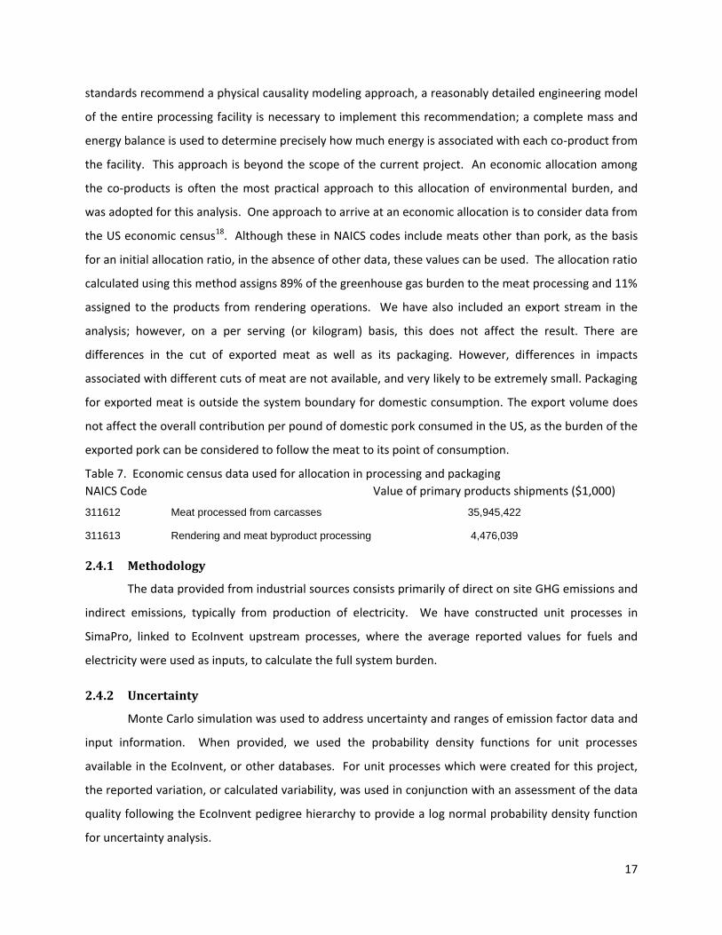
Table 7. Economic census data used for allocation in processing and packaging

NAICS Code

Value of primary products shipments ($1,000)

311612 Meat processed from carcasses 35,945,422

311613 Rendering and meat byproduct processing 4,476,039

2.4.1 Methodology

The data provided from industrial sources consists primarily of direct on site GHG emissions and

indirect emissions, typically from production of electricity. We have constructed unit processes in

SimaPro, linked to EcoInvent upstream processes, where the average reported values for fuels and

electricity were used as inputs, to calculate the full system burden.

2.4.2 Uncertainty

Monte Carlo simulation was used to address uncertainty and ranges of emission factor data and

input information. When provided, we used the probability density functions for unit processes

available in the EcoInvent, or other databases. For unit processes which were created for this project,

the reported variation, or calculated variability, was used in conjunction with an assessment of the data

quality following the EcoInvent pedigree hierarchy to provide a log normal probability density function

for uncertainty analysis.

18

2.4.3 Electricity

There are three electricity production regions in the U.S.; these regions are Eastern

Interconnection, Western Interconnection, and the Electric Reliability Council of Texas (ERCOT)

Interconnection19. Use of the three main interconnections as the basis for calculating environmental

burdens from electricity production are better than national, state, or even utility-level emission factors

because there is virtually no electricity energy transfer between the interconnect grids, so at this level

there is some certainty about the actual fuel mix used to provide electricity. In practice, for this model,

we generally do not know which the appropriate grid region is, and therefore, with the exception of

regional crop production have used the US national primary fuel mix for calculation of GHG emissions

associated with electricity consumption. In addition, while we have used US primary electricity unit

processes for foreground processes (those created for this project), we have not modified the entire

EcoInvent database, and thus most background processes are still linked to EU electricity processes.

2.4.4 Fuel Energy

Ecoinvent fuel energy unit process emissions include pre-combustion (that is emissions from

production and delivery of the fuel) and on-site combustion. The majority of fuel energy in pork

processing comes from natural gas and electricity.

Emissions from transportation were calculated using EcoInvent unit processes combined with

industry estimates for haul distances for feed to milling and from the mill to the farm. Industry reported

fuel consumption was used to estimate transportation mileage, which is the basic unit for consumption

of transportation fuels in the EcoInvent database.

2.4.5 Packaging Materials

For retail distribution in the United States, most meats, including pork, are packed on a

polystyrene plate with an absorbent pad and wrapped with a stretch wrap plastic film. We have

estimated 8.8 g of polystyrene20 and ½ g of stretch wrap material per pound of packaged pork. The

specific makeup of absorbent pads is generally proprietary. We used information in a patent21 to

represent a typical absorbent pad made from Vicose and expanded Vicose as the basis for the

calculations.

2.5 Retail

After distribution from the processor to the retail gate, pork is displayed for consumer purchase.

During this phase, there are four distinct emissions streams: refrigerant leakage, refrigeration electricity,

19

store overhead electricity and fuel (natural gas). Estimates of the sales volume, space occupancy, and

energy demands of pork were used to determine the burden of this supply chain stage. Overhead

electricity demand activities allocated to pork include ventilation, lighting, cooling, space heating, water

heating, and other miscellaneous electrical loads (e.g., free standing refrigerators). Based on the 2007

National Meat Case Study22 pork products occupy 19 - 20% of shelf space in the meat/poultry/fish

category; based on a combination of information from the Food Marketing Institute (price data) and

meat sales volumes (USDA), we estimated that 21.5% of meat sales. Using this information in

combination with data from the Food Marketing Institute23 on the fraction of grocery sales by

department and the average supermarket size, we calculated that pork represents approximately 2.7%

of typical supermarket sales and 6.3% of refrigerated sales. These fractions were used as allocation

fractions for refrigerated space. Buzby et al., in a study on the loss of perishables in supermarkets,

reported average loss of pork is 4.4%24. We also evaluated the allocation of retail emissions on a space

occupied basis. Information from a proprietary study reports that approximately 57 linear feet of

refrigerated shelf space is devoted to pork products in a typical grocery configuration with a total of

4300 refrigerated linear shelf feet and 21980 linear feet of total shelving. This results in 1.32% of total

refrigerated store shelving and 0.258% of total shelving space. We have included a sensitivity analysis of

these allocation approaches (economic and physical) § 3.4, Figure 14.

2.5.1 Refrigerated Space Burden

The storage and sales of pork to the retail consumer carries a GHG burden from energy use

(electricity and natural gas), and fugitive emissions associated with refrigerant loss. Based on average

store square footage, consumer-facing shelf space, and end-use energy demands25,26,27, average

electricity, refrigerant, and natural gas activity flows per lb pork sold were developed. An average yearly

loss of refrigerants was included in the GHG emissions estimate25,27. R22 and R404A were assumed to

be used at 54% and 46%, respectively25.

2.6 Consumer

Impacts accounted in this phase include transport from retail to home, refrigeration and cooking

energy and food loss or waste. Consumer transportation related emissions were allocated using the

same economic and space based allocation fractions (whole store allocation basis – 0.258% with an

assumed 5 mile round trip for grocery store purchases). The fundamental assumption in this allocation

approach is that the composition of the products on supermarket or grocery store shelves is an

approximation of the average US household purchasing and storage. We also took either the economic

20

or shelf space estimates from supermarket refrigerated space as the allocation fractions for in-home

refrigeration electricity. Estimates of the consumer cooking energy for gas and electric ovens were

made. Cooking energy requirements were estimated using information from the US EPA Energy Star

program. Both pre-heat and cooking times were included, but assumed no additional idle time. Also

assumed was that the cooking energy was based on cooking eight 4-ounce servings (e.g., as a 2 pound

tenderloin to be cut into individual servings after being cooked). Cooking yield for pork depends on the

method, but ranges from 71 to 75%28,29. The Economic Research Service of the USDA provides annual

estimates of loss-adjusted food availability. The estimated loss at consumer phase is 39%; some current

research suggests that this may be closer to 29%30. This includes spoilage, plate waste, and cooking

weight loss. As indicated above there is a 21 to 25% weight loss due to cooking, and we have not

included this weight loss in the model calculations; we assumed a combined 10% spoilage and plate loss.

2.6.1 Post-Consumer Solid Waste

There is a relatively small quantity of post-consumer waste generated, and it is modeled using

an EcoInvent process for landfill disposal. We estimated the potential methane emission from meat

disposed in landfills using information reported by Cho and Park31. The elementary flow estimate from

these data is 0.344 lb CH4 per lb volatile solids disposed. Cooked pork meat is 97% volatile solids. This

estimate likely represents an upper limit to the methane generated when meat is disposed in landfills

because the study was focused on energy recovery from anaerobic digestion, and did not replicate

conditions in a landfill.

2.7 Software, Database and Model Validation

The LCA model was created using the SimaPro Software system for life cycle engineering,

developed by Pre, a Netherlands based company. The EcoInvent database was used for the life cycle

inventory data of the raw and process materials needed for background processes. All computational

modules are documented with reference citations to external source data also available in the literature

review5.

3 Scan level carbon footprint results

The model for the footprint is based on a 2 barn system: Breeding/Gestation/Lactation barn (or

Sow Barn) followed by a Nursery/Finish (N/F) barn. We recognize that this is not representative of all

configurations; however, addition of a third nursery barn and changing the N/F barn to a Grow/Finish

barn will have relatively small impact in terms of a high level scan. Transportation of animals between

21

the nursery and grow-finish barns will be the major additional source of emissions in this case. The

model is built to account for an entire life cycle of a single sow, and specifically includes gilt

development and multiple litters (parities). The N/F barn accounts for all the piglets from all parities

grown to full weight. Tables 1 through 4 present the model diets.

3.1 Life Cycle Phases

The model follows the structure shown in Figure 2. Each unit process, or stage, has inputs and

outputs that contribute to calculation of the overall GHG emissions of the system. The model

parameters are listed in Tables A-1 and A-2. In the following sections, we present the overall footprint

and several gate-to-gate partial footprints to provide a reference to other published LCA results.

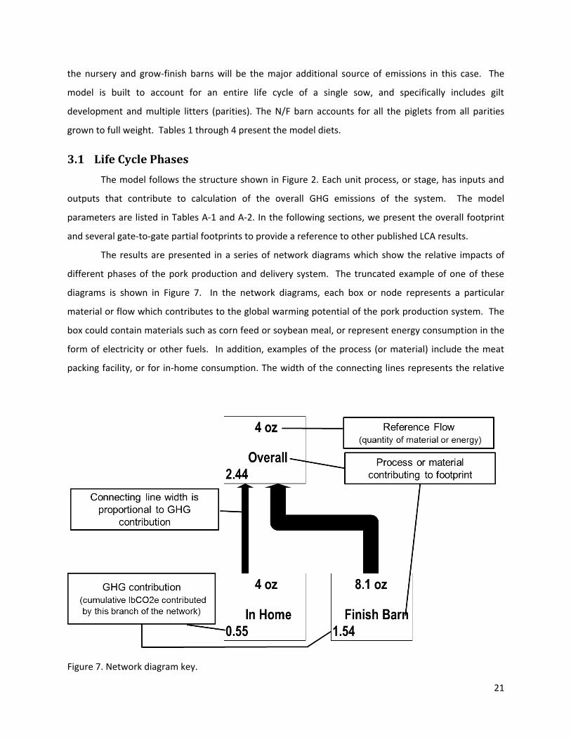
The results are presented in a series of network diagrams which show the relative impacts of

different phases of the pork production and delivery system. The truncated example of one of these

diagrams is shown in Figure 7. In the network diagrams, each box or node represents a particular

material or flow which contributes to the global warming potential of the pork production system. The

box could contain materials such as corn feed or soybean meal, or represent energy consumption in the

form of electricity or other fuels. In addition, examples of the process (or material) include the meat

packing facility, or for in-home consumption. The width of the connecting lines represents the relative

Figure 7. Network diagram key.

22

contribution from the particular unit to the whole global warming impact. The contribution shown in

each box is the cumulative contribution from all of the network nodes upstream in the supply chain plus

the contribution occurring at that node. Note that the reference flows do not necessarily represent

material or energy balances for the pork functional unit, and therefore may not sum to the value of the

reference flow of the receiving process.

Table 8 presents a list of the node names used in the network diagrams along with a definition

describing the materials or process which are encompassed by that node. Tables B-1 and B-2 in

Appendix B present a list of the parameters used in the model to characterize the base case system.

3.2 Overall Cradle-to-Grave GHG emissions.

Figure 8 and present the breakdown of the domestic pork supply chain GHG emissions. In

Figure 8, each major supply chain stage has been subdivided into the primary contributing activities. The

categories presented capture the supply chain activities that are unique to each stage of the supply

chain. The chemicals classification does not include fertilizers, which are accounted for in the feed bar.

The electricity shown at each level is the direct electrical contribution from that phase, thus electricity

Table 8 Unit Process Names and Descriptions for Network Diagrams

Cooking Includes energy for oven preheat and cooking

Corn Feed Combination of feed produced in different regions

Corn Grain Production of crops (region specific)

DDGs Dry Distillers Grains – includes allocation from ethanol production

Deep Pit Includes emissions associated with deep pit manure management system

Electricity Includes fuel mix, production, and distribution

Finish Barn Includes Nursery and Finish barn operations

In Home Includes transport from retail, in-home electricity for refrigeration and cooking burden

Lagoon Includes emissions associated with lagoon manure management system

Natural Gas Production, delivery, and combustion

Nitrogen Natural mix of nitrogen fertilizer production

Overall Cradle to grave; top level process

Processing Includes all processes from farm gate to preparation of carcass for packaging

Packaging Includes preparation of meat cuts and packaging on Styrofoam boat

Refrigerants Includes production and fugitive emissions

Retail Includes electricity for refrigeration, a share of store overhead electricity, and fugitive refrigerant emissions

Sow Barn Includes facilities used for breeding, gestation, and lactation

Soy Meal Includes processing of soybeans to oil and meal co-products

Soybeans On-farm production of soybeans

23

for crop irrigation is included in the feed bar. For each barn phase shown, the manure management is

the largest single contributor. In combination with Figure 9, it is apparent that much of the remaining

contribution is associated with production of the animal’s rations. Piglets are not included (contrast

with Figure 1) as s separate bar in the finish barn as that is the simply the contribution of the sow barn.

The primary contribution from retail and home consumption is associated with electricity used

for refrigeration, with some loss of refrigerants at retail; in addition, the waste emission at consumption

includes an estimate of the methane released from landfill disposal of spoiled and plate waste meat.

Because it is a legal requirement that refrigerants be captured from disposed household refrigerators,

we have assumed that there is no significant GHG emissions associated with end of life appliance

disposal.

In this analysis, we have not included weight loss on cooking, which can range between 20 to 30

percent due to a combination of water evaporation and loss of fat28,29. The USDA ERS is in the process of

revising, from 39% to 29%, the consumer phase loss of pork due to the combination of cooking weight

loss, spoilage, and plate loss (cooked, but discarded)30. Based on the proposed revision to consumer

Figure 8. Cumulative GHG emissions associated with consumption of pork in the US. The legend entries are discussed in the text. The estimates in this analysis do not include GHG emissions from pork destined for overseas consumption or food service industry emissions.

24

waste rates and the fact that weight loss during cooking does not induce additional production in the

supply chain, we have used an estimated value of 10% for consumer phase waste. The overall

cumulative GHG emissions for consumption of one 4-oz serving of US domestic pork based on reported

manure management practices and accounting for an assumed 10% waste of product by consumers is

2.48 lb CO2e. This model assumes a gas oven is used for cooking in the home; if in-home cooking is by

an electric oven, the overall impact increases to 2.54 lb CO2e per 4oz serving.

3.3 Scenario Analysis:

A series of scenarios are presented with alternate LCA models. The purpose of these alternate

models used to highlight the impact that some choices have on results of the carbon footprint. These

scenarios are focused on ration and manure management options at the live animal production phase of

the supply chain. Scenarios for the post-farm supply chain are also presented. In addition to scenario

testing, we conducted a sensitivity analysis.

The sensitivity of results to the main model parameters can be analyzed by adjusting parameters

up and down 10 percent and observing the change in the model result. Thus, the sensitivity of the LCA

to the most important input parameters can be evaluated.32 These analyses can be used to target data

collection, identify sources of improvement in process or analytical resolution, and to validate structures

of LCAs. Sensitivity analysis is important for conducting a consistency check on the model/LCA.

3.3.1 Animal Rations

Biofuels are a significant factor in US agriculture, and corn ethanol is a particularly important

contributor of distiller’s grains to animal husbandry. Although at present, only approximately 1% of the

distillers grains produced in the United States annually are fed to swine, the nutrient characteristics are

favorable and the usage of distiller's grains in the swine production industry is expected to increase in

future33. Evaluation of the difference in carbon intensity of different rations is therefore important. As

models that account for the manure characteristics with different rations are created, this will be an

even more important area of study.

25

A

B

Figure 9. A: Percentage contribution of the major life cycle stages for consumption of pork. Analysis is based on the national average manure management profile, and assumes gas oven cooking. B: GHG emissions from the supply chain. Values in the lower left corner of each box are lbs CO2e per 4oz serving prepared for consumption.

26

Figure 10 presents a comparison of rations which include or exclude distiller’s grains. There is

an approximately 6% reduction in the overall footprint when distiller’s grains are not included in the

ration. The additional processing of the corn to produce ethanol and DDGs results in DDGs having a

larger GHG emissions profile than corn grain or soy meal. This is true for both wet and dry DDGs

because approximately twice the mass of wet (~50% dry matter) DDGs is required to provide the same

nutrient density as a ration using dry DDGs (~92% dry matter), and this approximately offsets the energy

used for drying, that is, on a per lb (as-fed) basis, dry DDGs have double the footprint due to additional

energy for drying, but only ½ the mass (as-fed) is necessary to provide the same nutritional content to

the ration. UA swine specialists indicated that the majority of DDGs used are dry, rather than wet. The

slightly larger bar for feed in the no-DDG case arises from an allocation decision in the model.

Specifically, because of the economic allocation used at the distillery (98.3% allocation of the incoming

corn to ethanol), the change from DDGs to a corn soy mixture results in higher footprint of those feeds.

3.3.2 Regional Analysis

Based on the information presented in Table 5 and region-specific Simapro simulations the

Figure 10 Comparison of lifecycle emissions with or without DDGs included in the ration. The rations were modeled to provide necessary energy and protein content. Most categories are similar except for energy consumption, which is larger when DDGs are included in the diet.

27

cumulative GHG emissions associated with live animal production (cradle to farm gate) by USDA

production region are presented in Figure 11. Two factors are principally responsible for the differences

between regions: first, and most important, is the number of animals sold to market in each region, and

second is differences in the manure management profiles typical of the region. This is discussed in a

later section.

Figure 12 presents a comparison of the five manure management practices reported by in the

EPA GHG inventory13. In these comparisons, the only parameter changed was the type of manure

management used for each of the barns modeled. The ‘piglet’ contribution is different between the

scenarios as a result of the manure management. It is not surprising that anaerobic lagoons make a

larger contribution to GHG emissions than other management options. It is interesting to note that the

Figure 11. Cumulative metric tons of CO2e associated with pork production in the U.S. These estimates are based on federally inspected units reported for the regions shown in the legend. The total boneless weight estimated from these data correlate very closely to the per capita pork consumption reported by the Economic Research Service (47 lb/person/year). This analysis does not account for the structure of the industry where sow operations are not necessarily near the nursery finish operations. For purposes of this analysis, the sow operation footprint was estimated as coming from the same region as the finished animals. The region and production weighted national average carbon footprint is 2.87 lb CO2e per lb live weight at the farm gate (equivalent to 3.83 lb/lb dressed carcass or 5.9 lb CO2e/lb boneless meat).

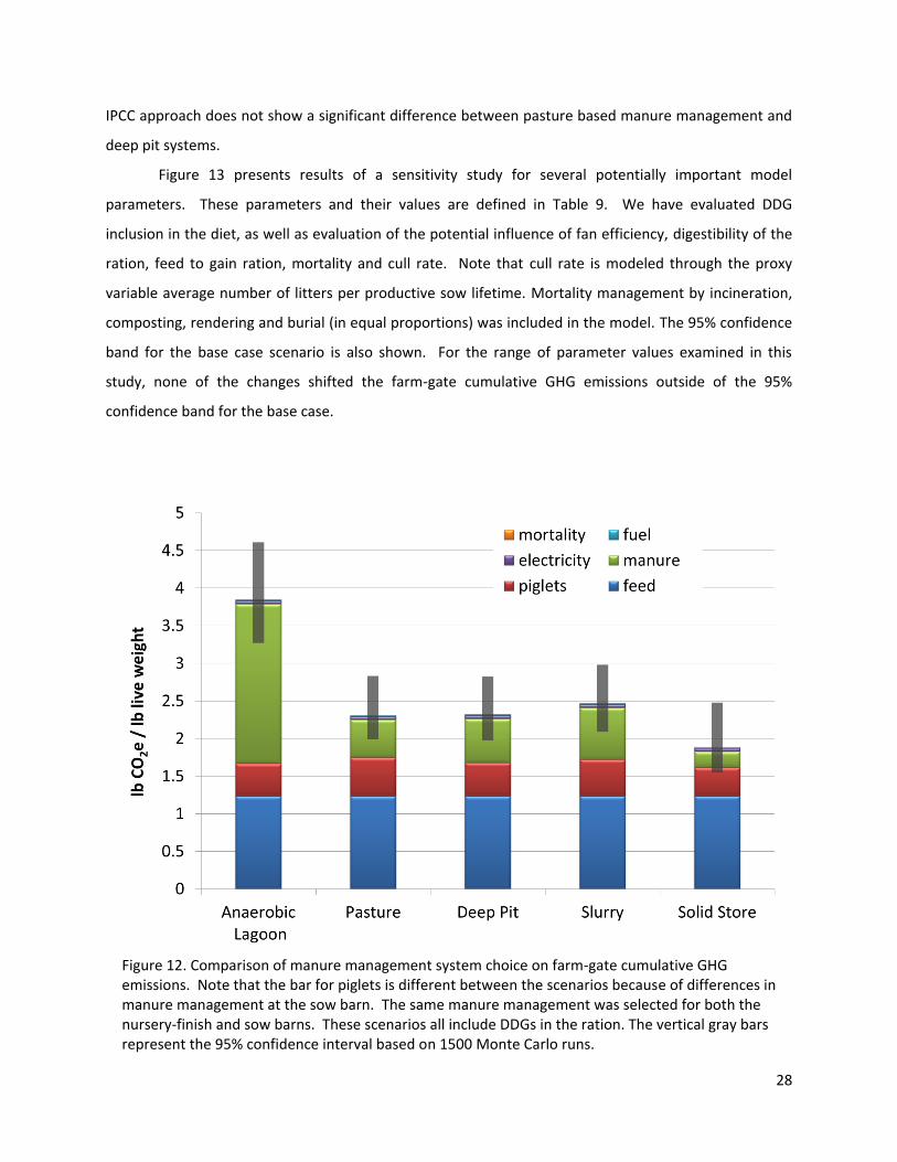
28

IPCC approach does not show a significant difference between pasture based manure management and

deep pit systems.

Figure 13 presents results of a sensitivity study for several potentially important model

parameters. These parameters and their values are defined in Table 9. We have evaluated DDG

inclusion in the diet, as well as evaluation of the potential influence of fan efficiency, digestibility of the

ration, feed to gain ration, mortality and cull rate. Note that cull rate is modeled through the proxy

variable average number of litters per productive sow lifetime. Mortality management by incineration,

composting, rendering and burial (in equal proportions) was included in the model. The 95% confidence

band for the base case scenario is also shown. For the range of parameter values examined in this

study, none of the changes shifted the farm-gate cumulative GHG emissions outside of the 95%

confidence band for the base case.

Figure 12. Comparison of manure management system choice on farm-gate cumulative GHG emissions. Note that the bar for piglets is different between the scenarios because of differences in manure management at the sow barn. The same manure management was selected for both the nursery-finish and sow barns. These scenarios all include DDGs in the ration. The vertical gray bars represent the 95% confidence interval based on 1500 Monte Carlo runs.

29

3.4 Post farm supply chain

We performed a similar scenario analysis for post-farm supply chain model parameters. These

parameters are given in Table 10; as a test of sensitivity of the results to variation in the parameter

values, we have taken a plus/minus range of 10% of the baseline value, and the results shown in Figure

14. The range of GHG emissions associated with the high and low parameter combinations remain

within the 95% confidence interval estimate for the base case (mean). The trends identified in these

scenarios suggest that while improvements are possible that significant reductions in the sector’s overall

GHG emissions will be derived from on-farm innovation. Again, the expected range of emissions is

captured effectively by the 95% confidence bands that result from the Monte Carlo simulation.

Table 9. Cradle to farm gate sensitivity parameters. Each row has parameters for a simulation. Shaded cells were the only parameter changed during each run (defined by a row).

Model Parameter

Scenario

Digestible Fraction

Conversion Efficiency

Finish /Sow Mortality

Live Piglets / litter

CFM / watt

Average Parities / Sow

CFM / sow

CFM / pig

Base Case 0.82 1 4 9.5 0.012 3.5 200 60

Low Digest 0.738 1 4 9.5 0.012 3.5 200 60

High F/G 0.82 1.05 4 9.5 0.012 3.5 200 60

Low F/G 0.82 0.95 4 9.5 0.012 3.5 200 60

High Mortality

0.82 1 10 9.5 0.012 3.5 200 60

Low Mortality

0.82 1 2 9.5 0.012 3.5 200 60

Low Piglet Mortality

0.82 1 4 10.45 0.012 3.5 200 60

High E Fan 0.82 1 4 9.5 0.0108 3.5 200 60

Low E Fan 0.82 1 4 9.5 0.0132 3.5 200 60

High Litter 0.82 1 4 9.5 0.012 3.85 200 60

Low Litter 0.82 1 4 9.5 0.012 3.15 200 60

Low Ventilation

0.82 1 4 9.5 0.012 3.5 180

54

High Ventilation

0.82 1 4 9.5 0.012 3.5 220 66

30

3.4.1 Meat Processing

Figure 15 presents the details of the meat processing stage of the supply chain. The most

significant contributors are natural gas and electricity. The diesel shown represents the fuel consumed

in transport of live animals to the processing and packaging plant. Despite the relatively low

contribution to the supply chain, there is still a large amount of energy and GHG emissions associated

with processing and continued efforts to increase efficiency both for cost savings and reduction in GHG

emissions are warranted.

Figure 13. Sensitivity analysis for farm gate production. Reported on a boneless meat basis

Table 10. Parameters evaluated in post-farm gate scenario testing. Scenario Parameter Value

Low Mean High

Cooking Gas Gas Electric

Allocation of consumer electricity 0.0117 0.013 0.0143 Annual consumer refrigeration electrical usage (kWh) 1213 1348 1483

In-home product waste 0.09 0.1 0.11

Retail loss fraction 0.0396 0.044 0.0484

Boneless fraction of carcass 0.7 0.65 0.6

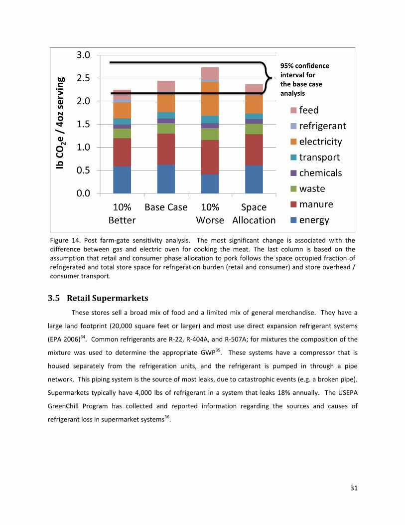
31

3.5 Retail Supermarkets

These stores sell a broad mix of food and a limited mix of general merchandise. They have a

large land footprint (20,000 square feet or larger) and most use direct expansion refrigerant systems

(EPA 2006)34. Common refrigerants are R-22, R-404A, and R-507A; for mixtures the composition of the

mixture was used to determine the appropriate GWP35. These systems have a compressor that is

housed separately from the refrigeration units, and the refrigerant is pumped in through a pipe

network. This piping system is the source of most leaks, due to catastrophic events (e.g. a broken pipe).

Supermarkets typically have 4,000 lbs of refrigerant in a system that leaks 18% annually. The USEPA

GreenChill Program has collected and reported information regarding the sources and causes of

refrigerant loss in supermarket systems36.

Figure 14. Post farm-gate sensitivity analysis. The most significant change is associated with the difference between gas and electric oven for cooking the meat. The last column is based on the assumption that retail and consumer phase allocation to pork follows the space occupied fraction of refrigerated and total store space for refrigeration burden (retail and consumer) and store overhead / consumer transport.

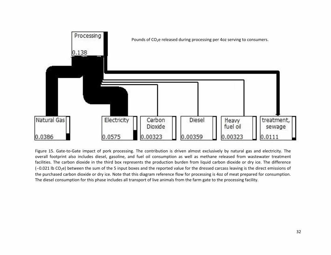
32

Figure 15. Gate-to-Gate impact of pork processing. The contribution is driven almost exclusively by natural gas and electricity. The overall footprint also includes diesel, gasoline, and fuel oil consumption as well as methane released from wastewater treatment facilities. The carbon dioxide in the third box represents the production burden from liquid carbon dioxide or dry ice. The difference

(~0.021 lb CO2e) between the sum of the 5 input boxes and the reported value for the dressed carcass leaving is the direct emissions of

the purchased carbon dioxide or dry ice. Note that this diagram reference flow for processing is 4oz of meat prepared for consumption. The diesel consumption for this phase includes all transport of live animals from the farm gate to the processing facility.

Pounds of CO2e released during processing per 4oz serving to consumers.

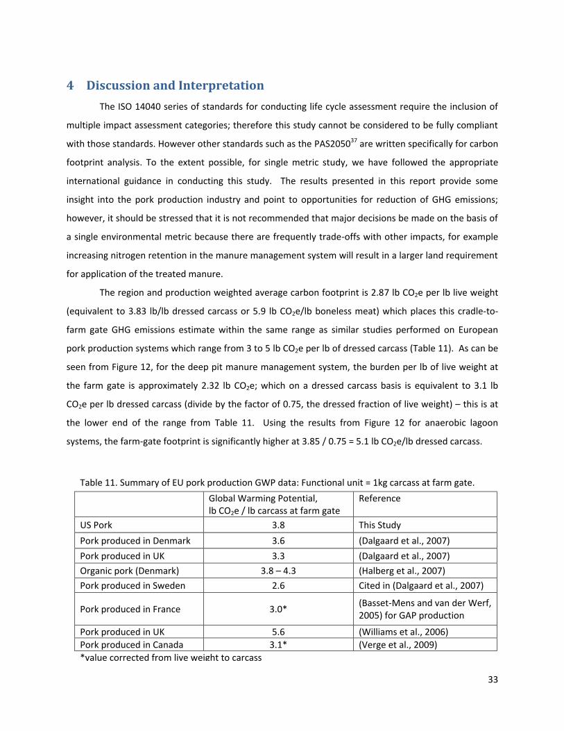
33

4 Discussion and Interpretation

The ISO 14040 series of standards for conducting life cycle assessment require the inclusion of

multiple impact assessment categories; therefore this study cannot be considered to be fully compliant

with those standards. However other standards such as the PAS205037 are written specifically for carbon

footprint analysis. To the extent possible, for single metric study, we have followed the appropriate

international guidance in conducting this study. The results presented in this report provide some

insight into the pork production industry and point to opportunities for reduction of GHG emissions;

however, it should be stressed that it is not recommended that major decisions be made on the basis of

a single environmental metric because there are frequently trade-offs with other impacts, for example

increasing nitrogen retention in the manure management system will result in a larger land requirement

for application of the treated manure.

The region and production weighted average carbon footprint is 2.87 lb CO2e per lb live weight

(equivalent to 3.83 lb/lb dressed carcass or 5.9 lb CO2e/lb boneless meat) which places this cradle-to-

farm gate GHG emissions estimate within the same range as similar studies performed on European

pork production systems which range from 3 to 5 lb CO2e per lb of dressed carcass (Table 11). As can be

seen from Figure 12, for the deep pit manure management system, the burden per lb of live weight at

the farm gate is approximately 2.32 lb CO2e; which on a dressed carcass basis is equivalent to 3.1 lb

CO2e per lb dressed carcass (divide by the factor of 0.75, the dressed fraction of live weight) – this is at

the lower end of the range from Table 11. Using the results from Figure 12 for anaerobic lagoon

systems, the farm-gate footprint is significantly higher at 3.85 / 0.75 = 5.1 lb CO2e/lb dressed carcass.

Table 11. Summary of EU pork production GWP data: Functional unit = 1kg carcass at farm gate.

Global Warming Potential, lb CO2e / lb carcass at farm gate

Reference

US Pork 3.8 This Study

Pork produced in Denmark 3.6 (Dalgaard et al., 2007)

Pork produced in UK 3.3 (Dalgaard et al., 2007)

Organic pork (Denmark) 3.8 – 4.3 (Halberg et al., 2007)

Pork produced in Sweden 2.6 Cited in (Dalgaard et al., 2007)

Pork produced in France 3.0* (Basset-Mens and van der Werf, 2005) for GAP production

Pork produced in UK 5.6 (Williams et al., 2006)

Pork produced in Canada 3.1* (Verge et al., 2009)

*value corrected from live weight to carcass

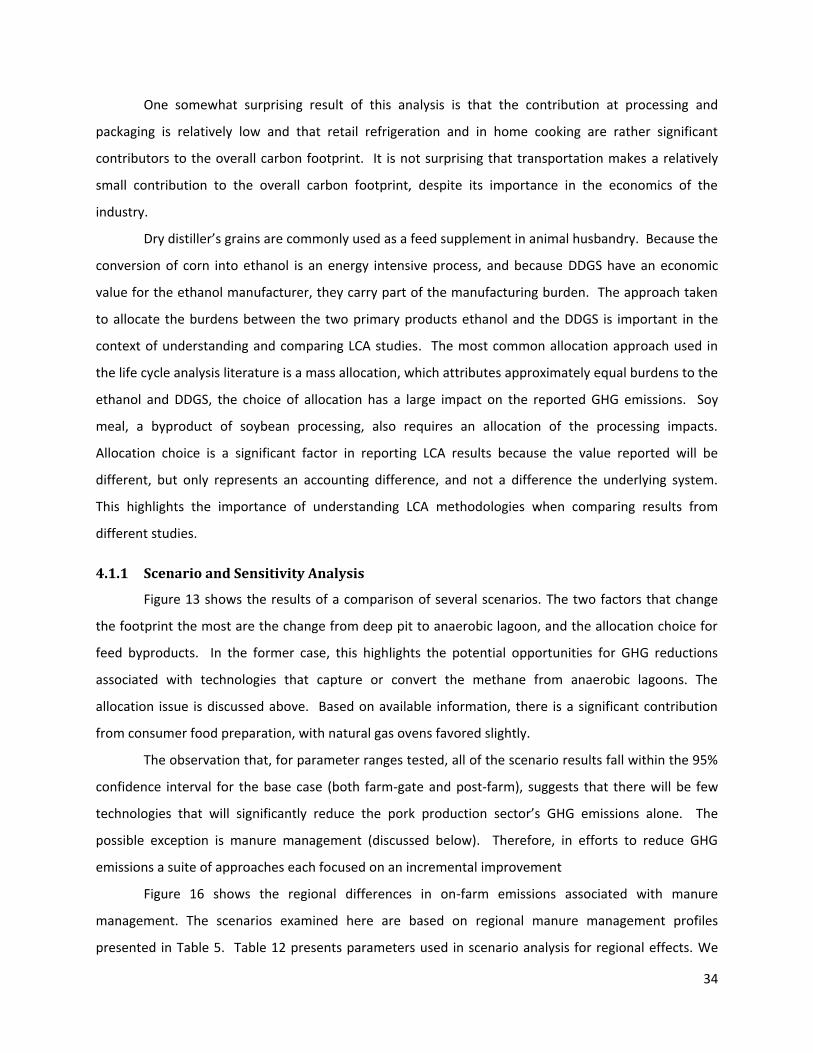
34

One somewhat surprising result of this analysis is that the contribution at processing and

packaging is relatively low and that retail refrigeration and in home cooking are rather significant

contributors to the overall carbon footprint. It is not surprising that transportation makes a relatively

small contribution to the overall carbon footprint, despite its importance in the economics of the

industry.

Dry distiller’s grains are commonly used as a feed supplement in animal husbandry. Because the

conversion of corn into ethanol is an energy intensive process, and because DDGS have an economic

value for the ethanol manufacturer, they carry part of the manufacturing burden. The approach taken

to allocate the burdens between the two primary products ethanol and the DDGS is important in the

context of understanding and comparing LCA studies. The most common allocation approach used in

the life cycle analysis literature is a mass allocation, which attributes approximately equal burdens to the

ethanol and DDGS, the choice of allocation has a large impact on the reported GHG emissions. Soy

meal, a byproduct of soybean processing, also requires an allocation of the processing impacts.

Allocation choice is a significant factor in reporting LCA results because the value reported will be

different, but only represents an accounting difference, and not a difference the underlying system.

This highlights the importance of understanding LCA methodologies when comparing results from

different studies.

4.1.1 Scenario and Sensitivity Analysis

Figure 13 shows the results of a comparison of several scenarios. The two factors that change

the footprint the most are the change from deep pit to anaerobic lagoon, and the allocation choice for

feed byproducts. In the former case, this highlights the potential opportunities for GHG reductions

associated with technologies that capture or convert the methane from anaerobic lagoons. The

allocation issue is discussed above. Based on available information, there is a significant contribution

from consumer food preparation, with natural gas ovens favored slightly.

The observation that, for parameter ranges tested, all of the scenario results fall within the 95%

confidence interval for the base case (both farm-gate and post-farm), suggests that there will be few

technologies that will significantly reduce the pork production sector’s GHG emissions alone. The

possible exception is manure management (discussed below). Therefore, in efforts to reduce GHG

emissions a suite of approaches each focused on an incremental improvement

Figure 16 shows the regional differences in on-farm emissions associated with manure

management. The scenarios examined here are based on regional manure management profiles

presented in Table 5. Table 12 presents parameters used in scenario analysis for regional effects. We

35

evaluated the GHG emissions for regional profiles of manure management with an appropriate average

annual temperature for each location. The main effects are associated with nitrous oxide and methane

from the manure management systems as shown below in comparison of the base case for each region.

The significantly larger emissions from Region 4 point to an opportunity for GHG emissions reductions

associated with a shift away from anaerobic lagoons.

There are additional uncertainties in calculation of a carbon footprint associated with the values

of emission factors used to predict the quantity of GHG emitted for a given management system. The

most sensitive parameters are the fraction of volatile solids in the manure available for conversion to

methane (B0), and the rates of nitrogen volatilization from the manure management system. The ranges

of these parameters are given in Table 12. The ranges selected are not intended to represent the full

range of possible values, but represent, in combination, three cases that demonstrate the range of

uncertainty associated with the IPCC emission factors.

The sensitivity results show that Region 4 has larger GHG emissions, approximately 1 and ½ lb

CO2e per lb live weight compared to Regions 5 and 7 respectively. This is primarily driven by increased

Table 12. Parameter ranges for manure management systems sensitivity analysis

Sensitivity Parameter Parameter function in model Low Mean High

Methane Conversion Potential

Fraction of volatile solids that could be converted to methane

0.41 0.48 0.52

Lagoon volatilization

Fraction of N lost by volatilization

0.32 0.4 0.48

Pasture volatilization 0.24 0.3 0.36

Deep pit volatilization 0.2 0.25 0.3

Liquid slurry volatilization

0.41 0.48 0.52

Solid store volatilization 0.4 0.45 0.5

Lagoon leaching Fraction of N lost by leaching into the ground

0.0025 0.005 0.01

Slurry leaching 0.0025 0.005 0.01

Deep pit leaching 0.0025 0.005 0.01

Pit direct N2O Fraction of N converted directly to N2O

0.001 0.002 0.004

Slurry direct N2O 0.0025 0.005 0.01

Indirect N2O (volatilized) Fraction of N converted to N2O

after loss from MMS

0.005 0.01 0.02

Indirect N2O (leached) 0.0075 0.0075 0.0075

Field Application Fraction of N converted to N2O after land application (inorganic fertilizer and plant residue)

0.004 0.0208 0.061

36

methane production as a result of higher average annual temperature and higher adoption rate of

anaerobic lagoons for manure management. The large difference in the feed contribution to the

footprint is associated, primarily, with the large uncertainty in the nitrous oxide emission rates

associated with nitrogen fertilizer application (Table 12). The 95% confidence band for the base case is

shown as a gray bar. In all three regions, the 95% confidence band is approximately the same as the

expected range of emissions. In region 4, the feed and manure contributions are approximately equal,

while in the other regions, feed is a more significant contributor to GHG emissions than manure

management. This is the result of a larger proportion of anaerobic lagoons in region 4 combined with

slightly lower average annual temperatures in the other two regions. The primary reason for differences

in the feed contribution between scenarios in a region is the sensitivity to the N2O emission factor for

field application of nitrogen and crop residues.

4.2 Data Quality, Uncertainty and Reconciliation

4.2.1 Uncertainty in Input Variables

All data points have some uncertainty about them. The higher the uncertainty associated with

an input variable, the less certain any results derived from that variable. Sources of uncertainty are a

function of many facets of data, including reliability of measurements, sample size relative to total

populations, representativeness of the sample, geographic variability, and many other characteristics.

Sources of uncertainty can generally be categorized as variability and knowledge uncertainty.38

Variability is the inherent noisiness of a system, the stochastic nature of a process. An example would

be rainfall intensity; no matter how much you measure rainfall intensity, it will still vary over time and

space because rainfall is inherently variable, though the characterization of the distribution of probable

outcomes can be enhanced. Knowledge uncertainty is a measure of our ignorance of a system; it could

be defined, given knowledge about the system, but those data are not available for the given analysis.

Each type of uncertainty exists in any complex analysis, especially in LCA. The major sources of

uncertainty in LCA are knowledge uncertainty associated with LCI data. Honest assessment of the

impact of LCA requires quantifying both types of uncertainty in the output.

4.2.2 Monte Carlo Simulation

Propagation of uncertainty in mathematical models such as life cycle analyses are frequently

performed using a process of iterative random sampling commonly called Monte Carlo simulation. The

process is very simple in concept: a variable or set of variables in an equation are represented as

distributions rather than discrete numbers. These distributions can be as simple as a uniform

37

distribution, where the variable has an equal probability of being any number between a minimum and

a maximum. They can be more complex such as a log-normal probability distribution, bounded by zero

and positive infinity. Each time the model is executed (iteration) the software randomly selects from the

assigned distribution for each variable (roles the dice, as it were), records the value, and calculates the

outcome (results). This process can be repeated thousands of times to create a distribution of outputs

rather than a single number. This allows the analyst to determine the probable outcome of a model or

scenario, based upon a critical assessment of uncertainty about the inputs. Other techniques for

propagation of uncertainty in LCA exist39,40,41; however, in this study Monte Carlo Simulation was used.

4.2.3 Assigning Distributions to Variables

Each of the model parameters as well as values of other input parameters has been assigned a

probability density function which represents our best estimate of the potential range for that

parameter. In addition to the basic or inherent variability in the system, we are following the EcoInvent

protocol for assigning a pedigree to these data. The pedigree matrix considers factors such as the

temporal and geographical relevance of the life cycle inventory data to the study at hand, the number of

samples, the validity of the data with regard to verification as opposed to expert judgment, and the

Figure 16. Comparison of regional differences and the effects of uncertainty in emission factors for manure management systems. Region 4 has a larger fraction of anaerobic lagoons than reported for regions 5 or 7, and thus has a markedly lager GHG emissions profile.

38

representativeness of the life cycle inventory data. Most of the distributions are considered to be log

normal, which prevents selection of negative values during the Monte Carlo simulations, and has the

added feature that the squared geometric standard deviation represents the 95% confidence band for

the distribution. 1500 Monte Carlo simulation runs were performed to assess the confidence band of

the estimated GHG emissions.

Variables in a model are assigned distributions based on a set of pre-determined criteria.

SimaPro provides four distribution choices: Range (uniform), triangular, normal, and log-normal. These

four distributions are adequate for propagation of knowledge uncertainty. A uniform distribution would

be applied to a variable where only the minimum and maximum range of possible values is known.

When a central tendency is known as well as the range, a triangular distribution can be applied. For

data with more than five observations, a normal or log-normal distribution can be applied. If the data

have a central tendency, normal distributions are appropriate. If there is an explicit lower bounded of

zero (very common in natural resources data) a log-normal distribution should be applied. We have

assigned uncertainty ranges to most variables; however there are some which have not been assigned.

In particular, variables that have been parameterized to allow sensitivity analysis do not have

distributions assigned as the Simapro software does not support this feature; the result of this limitation

of the software is that the range of uncertainty in the final result is underestimated. In addition most of

the allocation parameters are fixed because they are inter dependent and inaccurate simulations can

result.

4.2.4 Data Quality Assessment

We have adopted the EcoInvent pedigree approach for assigning data quality indicators.

Because most of the data for this project was derived from the literature, we have made estimated of

the base uncertainty prior to application of the pedigree matrix. The uncertainty distributions are not

based on extensive data collection, but on the best judgment of the research team and ranges observed

in the literature.

4.2.5 Consistency assessment

There are some additional points regarding consistency of the modeling that should be pointed

out. To the extent feasible we have used EcoInvent unit processes, used unit processes created at the

University of Arkansas for other LCA projects (most of the crop production information) or created new

unit processes specific to this project, however there were some instances where unit processes were

modeled with economic input output (EIO) data. Differences in system boundary particularly between

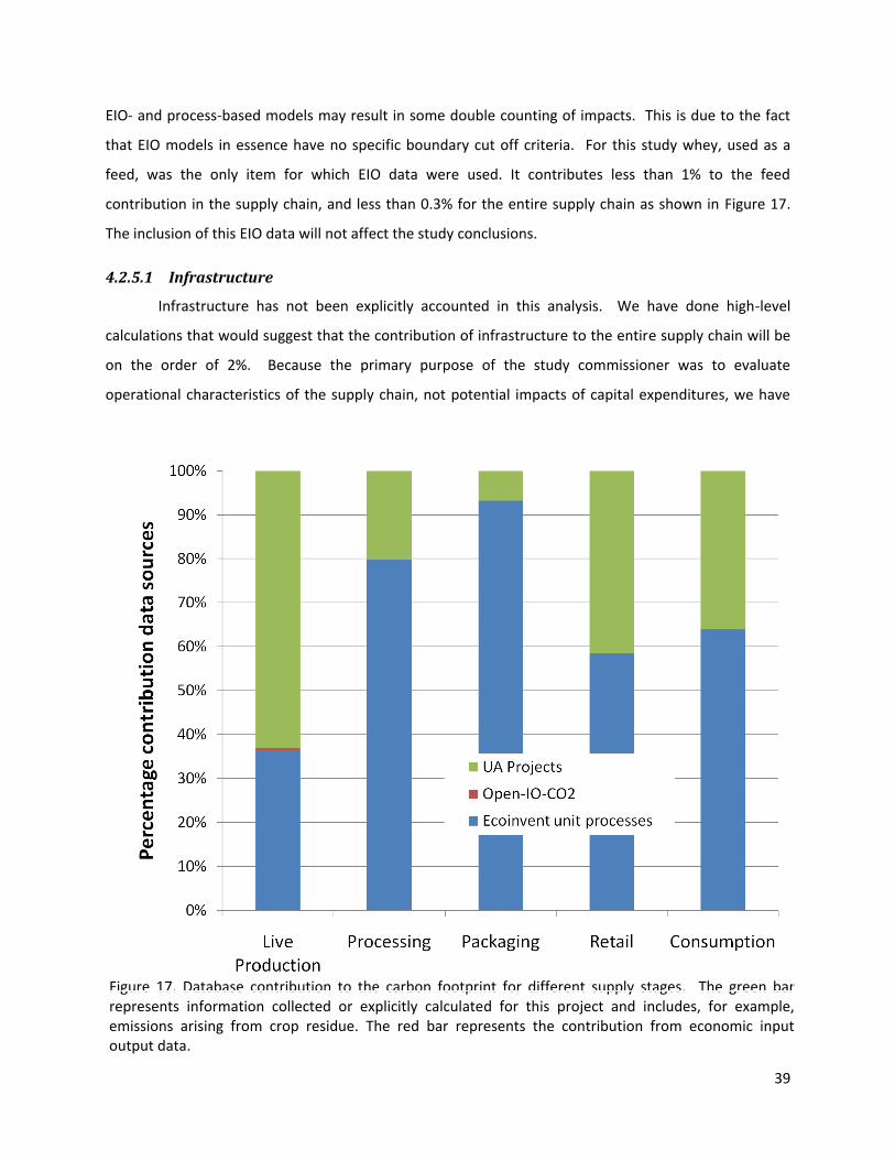
39

EIO- and process-based models may result in some double counting of impacts. This is due to the fact

that EIO models in essence have no specific boundary cut off criteria. For this study whey, used as a

feed, was the only item for which EIO data were used. It contributes less than 1% to the feed

contribution in the supply chain, and less than 0.3% for the entire supply chain as shown in Figure 17.

The inclusion of this EIO data will not affect the study conclusions.

4.2.5.1 Infrastructure

Infrastructure has not been explicitly accounted in this analysis. We have done high-level

calculations that would suggest that the contribution of infrastructure to the entire supply chain will be

on the order of 2%. Because the primary purpose of the study commissioner was to evaluate

operational characteristics of the supply chain, not potential impacts of capital expenditures, we have

Figure 17. Database contribution to the carbon footprint for different supply stages. The green bar represents information collected or explicitly calculated for this project and includes, for example, emissions arising from crop residue. The red bar represents the contribution from economic input output data.

40

excluded infrastructure because it is relatively small (although potentially just above the cut off

criterion). Thus the focus is to identify the opportunities for operational innovation. To ensure the

greatest degree of consistency possible regarding infrastructure, all unit processes used in the SimaPro

model were of type ‘U’ (unit) rather than type ‘S’ (system) so that when infrastructure processes are

excluded from the analysis, they are excluded over the entire lifecycle, including deep background

processes, compared to utilization of the integrated ‘S’ processes which were created with

infrastructure included. Since the model was constructed in this manner, and because the background

processes from the EcoInvent database do include infrastructure impacts, we performed a comparison

with and without the background process infrastructure to estimate the effect of excluding

infrastructure. The result of this analysis showed that including infrastructure impacts for background

processes increases the footprint by approximately 2%. The overall conclusions of the study are

unaffected by this because this impact is distributed throughout the supply chain, and the major impacts

are not shifted.

One potential consequence of not including infrastructure is that economies of scale associated

with large farming operations will not be completely captured because, in general, there are significant

efficiencies in capital expenditures with increasing size of the facility. Because this analysis did not

include the infrastructure burden, conclusions regarding the effect of farm size on the cumulative GHG

emissions must be made cautiously.

4.2.5.2 Allocation

We have used different allocation procedures at different stages in the supply chain. For

specific stages we have made every effort to apply the same allocation procedure uniformly to prevent

bias. As an example, for feed by products like grain meal and distiller’s grains we have applied an

economic value allocation for each of the byproducts; for scenario analysis, we compared to a uniformly

applied a mass allocation. In order to do this, for some products, we retrieved the multi-output process

from the EcoInvent web site and modified the default allocation fractions.

4.3 Model Validation

The LCA model was created using the SimaPro software system for life cycle engineering,

developed by Pre, The Netherlands. The EcoInvent database provides the life cycle inventory data for

upstream burdens of most of the raw and process materials used as inputs. Our goal is to provide a

transparent model for calculating the GHG emissions of the pork industry using a functional unit of 1

serving of pork consumed. All computational modules are documented with reference citations to

41

external sources. Spreadsheet computations are documented with the supporting logic. All formulas

have been checked by both the author of the module and at least one additional team member.

Because the intended audience of this study includes the general marketplace, an independent,

third-party critical review was conducted. In order to prepare a defensible GHG emissions baseline and

a transparent methodology that can be used to assess progress towards achieving a sustainable value

chain in the pork industry, it is important to have a consensus regarding the sources and types of data

used to develop the baseline, as well as general methodology.

5 Conclusions

In conclusion, the results of this scan analysis demonstrate that the mean value for cradle to

farm gate production of pork in the US is within the range reported in the literature for pork produced

elsewhere in the world, and is similar to other animal proteins. The results also show that both retail

and in-home electricity use for refrigeration are non-trivial contributions to the overall footprint, while

processing/packaging contributes a relatively smaller amount. Based on IPCC recommended

calculations, the deep pit system is preferred to anaerobic lagoons due to reduced methane production.

The issue of allocation of burdens for feeds is an important one regarding reporting of carbon

footprints, and it is recommended that a standard approach for handling agricultural byproducts like

soybean meal and DDGS be agreed upon across the industries involved. This national scale analysis

provides a baseline GHG emissions estimate against which the sector can benchmark future reductions.

Finally, the choice of manure management system is crucial in determining the carbon footprint.

The contribution of on-farm energy consumption represents about 25% of the farm contribution for

deep pit systems and only about 10% for anaerobic lagoon systems. The resolution of this scan does not

allow us to highlight clear energy saving opportunities; however, efforts at energy conservation are

simultaneously good for the environment and offer potential cost savings.

42

6 Literature Cited

1 Dong, H., Mangino, J., Mcallister, T., Hatfield, J. L., Johnson, D., Lassey, K. R., et al. (2006) Chapter 10 emissions from livestock and manure management. 2006 IPCC Guidelines for National Greenhouse Gas Inventories.

2 American Society of Agricultural Engineers, (2005) ASAE D384.2 MAR2005. Manure Production and Characteristics.

3 Purdue Pork Industry Handbook, (2009) Purdue University Extension Service, West Lafayette, IN 4 Forster, P., V. Ramaswamy, P. Artaxo, T. Berntsen, R. Betts, D.W. Fahey, J. Haywood, J. Lean, D.C. Lowe,

G. Myhre, J. Nganga, R. Prinn, G. Raga, M. Schulz and R. Van Dorland, (2007) Changes in Atmospheric Constituents and in Radiative Forcing. In: Climate Change 2007: The Physical Science Basis. Contribution of Working Group I to the Fourth Assessment Report of the Intergovernmental Panel on Climate Change [Solomon, S., D. Qin, M. Manning, Z. Chen, M. Marquis, K.B. Averyt, M.Tignor and H.L. Miller (eds.)]. Cambridge University Press, Cambridge, United Kingdom and New York, NY, USA.

5 Frank, Maxwell, and Thoma (2009) Greenhouse Gas Emissions and Global Warming Potential of the U.S. Swine Industry: Review of the Literature from a Life Cycle Perspective. www.npb.org

6 Kansas State Swine Nutrition Guide. 2007, http://www.ksre.ksu.edu/library/lvstk2/mf2301.pdf 7 H. H. Stein and G. C. Shurson. Board-Invited Review: The use and application of distillers dried grains

with solubles in swine diets. J Anim Sci 2009 87: 1292-1303. 8 USDA NASS, (2009) United States Department of Agriculture, National Agricultural Statistics Service,

Agricultural Chemical Usage Summary; Crop Production Summary, http://www.nass.usda.gov/ 9 http://agmrc.org/renewable_energy/ethanol/ethanol__prices_trends_and_markets.cfm, Accessed

March 2011 10 United Soybean Board, (2009) Data update of soybean and soy feedstocks production and life cycle

assessment of soy-based products and petroleum-based alternatives. Peer Reviewed Final Report. October, 2009.

11 De Klein, C., Novoa, R. S. A., Ogle, S., Smith, K. A., Rochette, P., Wirth, T. C., et al. (2006) “CHAPTER 11 N2O Emissions from Managed Soils and CO2 Emissions from Lime and Urea Application” in 2006 IPCC Guidelines for National Greenhouse Gas Inventories. IPCC.

12 American Society of Agricultural Engineers, (2005) ASAE D384.2 MAR2005 Manure Production and Characteristics.

13 USEPA (2009), Inventory of U.S. Greenhouse Gas Emissions and Sinks: 1990-2008; Annex A, Table 182. 14 West, T. O., & Six, J. (2006). Considering the influence of sequestration duration and carbon

saturation on estimates of soil carbon capacity. Climatic Change, 80(1-2), 25-41. doi: 10.1007/s10584-006-9173-8.

15 Christopher, S., & Lal, R. (2007). Nitrogen Management Affects Carbon Sequestration in North American Cropland Soils. Critical Reviews in Plant Sciences, 26(1), 45-64. doi: 10.1080/07352680601174830.

16 Johnson, J. M., Franzluebbers, A. J., Weyers, S. L., & Reicosky, D. C. (2007). Agricultural opportunities to mitigate greenhouse gas emissions. Environmental pollution (Barking, Essex : 1987), 150(1), 107-24. doi: 10.1016/j.envpol.2007.06.030.

17 West, T. O., & Marland, G. (2002). A synthesis of carbon sequestration, carbon emissions, and net carbon flux in agriculture: comparing tillage practices in the United States. Agriculture, Ecosystems & Environment, 91(1-3), 217-232. doi: 10.1016/S0167-8809(01)00233-X.

43

18 US Economic Census, Animal slaughter sector (31161), http://factfinder2.census.gov/ 19 Deru, M. and Torcellini, P., (2007) Source energy and emission factors for energy use in buildings,

Technical Report NREL/TP-550-38617, National Renewable Energy Laboratory, June 2007. 20 Genpak® (2011) polystyrene tray model number TR02P (7.8 lb/400 trays)

http://www.genpak.com/product/processor-supermarket-trays/ 21 Elves, J., Ley, S. J. (1985) Absorbent pads United States Chicopee (New Brunswick, NJ) 4551377

http://www.freepatentsonline.com/4551377.html 22 National Meat Case Study (2007)

http://www.porkretail.org/filelibrary/Retail/NMCS_execSum100710small.pdf 23 FMI, (2008) Supermarket Sales by Department – Percent of Total Supermarket Sales,

http://www.fmi.org/docs/facts_figs/grocerydept.pdf 24 Buzby, .J C., Wells,H.F., Axtman, B. and Mickey, J. (2009) Supermarket Loss Estimates for Fresh

Fruit, Vegetables, Meat, Poultry, and Seafood and Their Use in the ERS Loss-Adjusted Food Availability Data. EIB-44, U.S. Dept. of Agriculture, Econ. Res. Serv. March 2009, http://www.ers.usda.gov/Publications/EIB44/EIB44.pdf

25 USEPA (2005) Revised draft analysis of U.S. commercial supermarket refrigeration systems, U.S. EPA's Stratospheric Protection Division, November 30, 2005 http://www.epa.gov/Ozone/partnerships/greenchill/

26 Energy Information Administration, Commercial Building Energy Consumption Survey, (2003) http://www.eia.doe.gov/

27 Energy Star Grocery and Convenience Stores, Building Upgrade Manual, http://www.energystar.gov/ia/business/ EPA_BUM_CH11_Supermarkets.pdf

28 Hamouz, F., Batenhorst, J, Driskell, J. and Mandigo, R. (1996) Impact of Cooking Method on Quality of Boneless Pork Loin Roasts. http://digitalcommons.unl.edu/cgi/viewcontent.cgi?article=1183&context=coopext_swine.

29 Bertram, H. C., H. J. Andersen, A. H. Karlsson, P. Horn, J. Hedegaard, L. Nørgaard, and S. B. Engelsen (2003), Prediction of technological quality (cooking loss and Napole Yield) of pork based on fresh meat characteristics, Meat Sci., 65, 707-712.

30 Muth, M. K., Karns, S.A., Nielsen, S.J. Buzby, J.C. and Wells, H.F. (2011). Consumer-Level Food Loss Estimates and Their Use in the ERS Loss-Adjusted Food Availability Data, TB-1927, U.S. Dept. of Agr., Econ. Res. Serv. January 2011.

31 Cho, J.K., Park, S.C. and Chang, H.N. (1995) Biochemical methane potential and solid state anaerobic digestion of Korean food wastes, Bioresource Technology, 52:245-253

32 Bjorklund, A.E. (2002) Survey to Improve Reliability in LCA. International Journal of LCA 7(2): 62-72.

33 Distillers Grains In Livestock And Poultry Feeds (University of Minnesota) http://www.ddgs.umn.edu/overview.htm, accessed March 26, 2011

34 USEPA (2006) Emissions from the U.S. Transportation Sector 1990 – 2003, Office of Transportation and Air Quality (6401A), EPA 420 R 06 003, March 2006

35 http://www.refrigerants.com/refrigerants.htm 36 Whitman, K., Thomas-Arkema, C., O'Shea, K., Strickland, N., Vogl, R., Cunningham, S., et al. (2009).

GreenChill Best Practices Guideline Commercial Refrigeration Retrofits. Environmental Protection Agency. Washington, D.C.

44

37 PAS 2050:2008 Specification for the assessment of the life cycle greenhouse gas emissions of goods and services British Standards Institute ISBN 978 0 580 50978 0 http://www.bsigroup.com/upload/Standards%20&%20Publications/Energy/PAS2050.pdf

38 Ling, C. W. (1993) Characterizing Uncertainty: A taxonomy and an analysis of extreme events. MS Thesis, Systems Engineering Department, University of Virginia, Charlottesville, VA.

39 Heijungs, R., (2010) Sensitivity coefficients for matrix-based LCA, International Journal of Life Cycle Assessment, 15:511-520

40 Heijungs R, Tan RR. Rigorous proof of fuzzy error propagation with matrix-based LCI. The International Journal of Life Cycle Assessment. 2010;15(9):1014-1019. Available at: http://www.springerlink.com/index/10.1007/s11367-010-0229-7 [Accessed December 10, 2010].

41 Hong, J., Shaked, S., Rosenbaum, R.K., and Jolliet, O. (2010) Analytical uncertainty propagation in life cycle inventory and impact assessment: application to an automobile front panel. International Journal of Life Cycle Assessment 15:499-510.

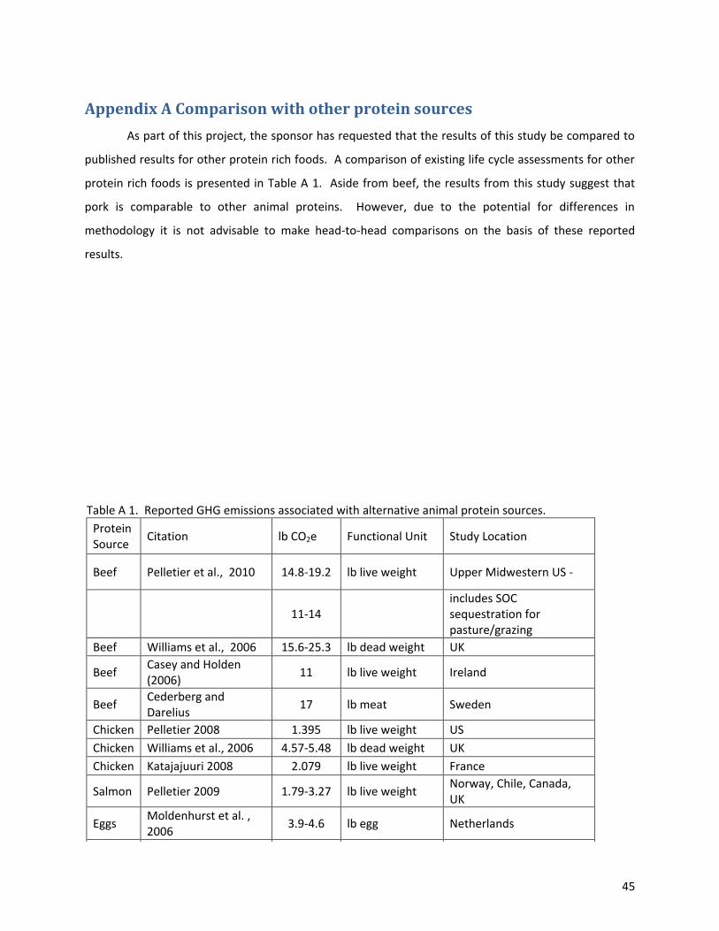
45

Appendix A Comparison with other protein sources

As part of this project, the sponsor has requested that the results of this study be compared to

published results for other protein rich foods. A comparison of existing life cycle assessments for other

protein rich foods is presented in Table A 1. Aside from beef, the results from this study suggest that

pork is comparable to other animal proteins. However, due to the potential for differences in

methodology it is not advisable to make head-to-head comparisons on the basis of these reported

results.

Table A 1. Reported GHG emissions associated with alternative animal protein sources.

Protein Source

Citation lb CO2e Functional Unit Study Location

Beef Pelletier et al., 2010 14.8-19.2 lb live weight Upper Midwestern US -

11-14

includes SOC sequestration for pasture/grazing

Beef Williams et al., 2006 15.6-25.3 lb dead weight UK

Beef Casey and Holden (2006)

11 lb live weight Ireland

Beef Cederberg and Darelius

17 lb meat Sweden

Chicken Pelletier 2008 1.395 lb live weight US

Chicken Williams et al., 2006 4.57-5.48 lb dead weight UK

Chicken Katajajuuri 2008 2.079 lb live weight France

Salmon Pelletier 2009 1.79-3.27 lb live weight Norway, Chile, Canada, UK

Eggs Moldenhurst et al. , 2006

3.9-4.6 lb egg Netherlands

Eggs Williams et al., 2006 0.62-0.68 per egg UK

46

Appendix B. Model parameters used for sensitivity and scenario

analysis Table B 2. Input parameters used for the base case scenario

Parameter Value Description

B_0 0.48 Fraction of VS available for conversion to methane

bgl_days 143 Breeding/Gestation/Lactation period (days)

meal_nf 1 lb/pig feed req'd per pig, nursery to finish, also used for gilt development

carcass_boneles 0.65 Carcass to boneless conversion

cfm_nf 60 cfm for ventilation in nursery-finish barn; Purdue handbook

cfm_sow 200 cfm for ventilation in sow barn; Purdue handbook

cfm_watts 0.012 Watts per cfm, assuming 0.1 inches water column pressure drop.

cons_alloc 0.013 (allocation of consumer refrigeration to pork products (approx. same as refrigeration space allocated to pork in supermarket refrigerated space - ignores items sold at ambient then refrigerated at home)

cons_pork 47.3 lbs pork consumed per capita in US (2005 ERS food availability data)

cons_refrig 1348 kWh/yr US household electricity used for refrigeration

cons_waste 0.1 Fraction of purchased meat disposed as waste

cooking 1 kWh to operate electric oven at 350

oF for 1 hour

http://michaelbluejay.com/electricity/cooking.html

days_in_nf 165 Nursery to finish - (days)

digest 0.82 Digestibility of feed; est. ASABE manure handbook

EF3_pit 0.002 IPCC emission factor for direct N20 from pit systems

EF3_slurry 0.005 IPCC emission factor for direct N20 from slurry systems

EF4 0.01 IPCC emission factor for N20-N from volatilized NH3-N

EF5 0.0075 IPCC emission factor for indirect N20 from leaching

fin_weight 268 Live weight, per pig, in lbs

hd_sow 1200 Number of sows in farrow - wean barn

heat_days 70 Heating days (dependent on average temperature)

leach_N_lagoon 0.005 IPCC fraction N lost through leaching

leach_N_pit 0.005 IPCC fraction N lost through leaching

leach_N_slurry 0.005 IPCC fraction N lost through leaching

live_carcass 0.75 Dressed carcass yield

N2O_residue 0.020821 kg N2O per kg N in crop residue

npg_sow 9.5 Number of piglets per litter

num_house 3 Number of people consuming pork per household

litter 3.5 Average number of litters per sow

sow_barn_area 7.5 Area (in square feet) of barn per animal, sow barn

sow_weight 450 Live weight (in pounds), sow, at cull

suppl_nf 8 lb/pig feed req's per pig, nursery to finish, including gilt development

suppl_sow 6 lb/pig feed req's per pig, nursery to finish, including gilt development

vol_nh3_lagoon 0.4 Fraction of NH3-N +NOx-N volatilized in lagoon mgmt systems

vol_nh3_pit 0.25 Fraction of NH3-N +NOx-N volatilized in lagoon mgmt systems

vol_nh3_slurry 0.48 Fraction of NH3-N +NOx-N volatilized in slurry mgt systems

vs_frac 0.8 Fraction of total manure solids that are volatile solids

weaned_weight 11 Weight of weaned piglet, entering nursery, in pounds

whey_nf 3 lb/pig feed requirement per pig, nursery to finish, also used for gilt development

0.48 fraction of VS available for conversion to methane

47

*Brumm, M. 2008. Hog Barns Don’t Come With Owner’s Manuals. Pork Congress 2008 Producer Education Seminars, Minnesota Pork

Producers Association. January 16-17

Table B 3. Calculated parameters

hd_nf hd_sow*npg_sow Nursery/Finish barn entering head for one parity

heat_litter 0.250*24*14 supplemental heat per litter (14 days heat needed ) kWh required per 250watts lamp (1 lamp per 2 sow)

light_sow 1.72*sow_barn_area*bgl_days* 24/1000

1.72watts/ft2;

lpg_gpd 100/5000*hd_nf Brumm, M.*

MCF_lagoon -0.000527*T_avg^2+0.026993* T_avg+0.449*1.1

CH4 conversion factor for lagoons manure systems IPCC Chap 10; Table 10A-7 10% correction factor to match Mangino (2001) which is the basis for the IPCC table.

MCF_pit_slurry Exp(T_avg*0.0884)*0.0712 CH4 conversion factor for liquid manure systems (both deep pit and liquid slurry systems) IPCC Table 10A-7

nf_barn_manure hd_nf*(corn_nf+sbm_nf+ddgs_nf)* (1-digest)

dry matter in manure (lbs); all nursery and finish (N/F) pigs for one parity

nf_barn_N 5.11*2.205*hd_nf pounds nitrogen excreted per finished animal litter; nursery + finish Table 18a ASABE

nf_barn_P 0.828*hd_nf*2.205 pounds phosphorus (same ref. as above)

sow_barn_manure hd_sow*(corn_sow+sbm_sow+ ddgs_sow)*(1-digest)

dry matter in manure (pounds); all sows breeding, gestation, and lactation (b/g/l), one parity

sow_barn_N hd_sow*bgl_days*0.117*2.205 0.117 kg/sow/day for 135 days b/g/l ASABE Table 18a converted to pounds

sow_barn_P 0.036*hd_sow*bgl_days*2.205 0.036 kg/sow/day for 135 days breeding, gestation, and lactation (b/g/l), ASABE Table 18a

vent_nf cfm_nf*cfm_watts*days_in_nf* 24/1000/.6/.8

Electricity (in kWh) for ventilation for 160 days in nursery and finish barns, fan efficiency 60%, motor efficiency 80%, per nursery and finish (N/F) pig

vent_sow cfm_sow*cfm_watts*bgl_days* 24/1000/.6/.8

Electricity (in kWh) for ventilation for 135 days in breeding, gestation, and lactation (b/g/l), fan efficiency 60%, motor efficiency 80%, per sow

48

Appendix C Third party critical review

First Round Critical Review Life Cycle Greenhouse Gas Emissions Baseline Study for the U.S. Pork Industry

Reviewers: please insert your comments in the second column of the table below, Indicating section, paragraphs and page in the first column.

Please use a new table cell for any new comment, to enable separate responses and action taken from authors to each individual comment. This

Appendix includes two rounds of review comments.

Comments and suggested changes by reviewers Response from author & Implemented changes

2.1 General comments

--- General comment 1

Please specify in the report that reviewers had access to the

model.

Response:

Action taken:

Added with description of review process § 2

--- General comment 2

The study is intended for communication to third parties, but

is not a comparative assertion. This confers some reporting

requirements (ISO 14044, §5.2). The following seem to be

missing for compliance:

description of cut-offs (not just the 1% rule used, but

what this meant in the actual study, e.g., which

elements were excluded, and also “de facto”

exclusions such as infrastructure);

description of effect of cut-offs on results;

quantitative description of unit processes (not all

available);

data quality assessment;

treatment of missing data (specifically, i.e., beyond

statement that “sometimes” IO data were used);

description of critical review process.

Response:

Action taken:

We have added a description of processes not included in the

analysis as a result of the cut-off criterion in §3.1.7.

We have also added §4.8 which includes the remaining information

required.

Description of review process included

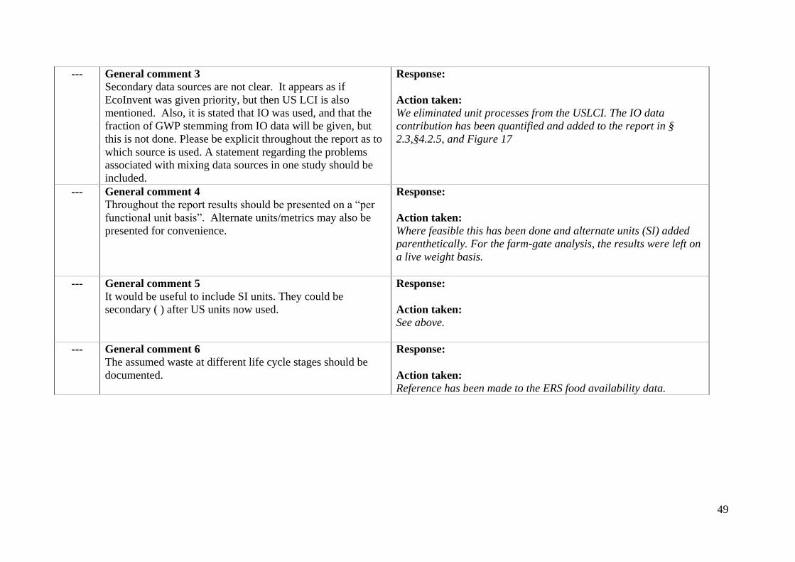
49

--- General comment 3

Secondary data sources are not clear. It appears as if

EcoInvent was given priority, but then US LCI is also

mentioned. Also, it is stated that IO was used, and that the

fraction of GWP stemming from IO data will be given, but

this is not done. Please be explicit throughout the report as to

which source is used. A statement regarding the problems

associated with mixing data sources in one study should be

included.

Response:

Action taken:

We eliminated unit processes from the USLCI. The IO data

contribution has been quantified and added to the report in §

2.3,§4.2.5, and Figure 17

--- General comment 4

Throughout the report results should be presented on a “per

functional unit basis”. Alternate units/metrics may also be

presented for convenience.

Response:

Action taken:

Where feasible this has been done and alternate units (SI) added

parenthetically. For the farm-gate analysis, the results were left on

a live weight basis.

--- General comment 5

It would be useful to include SI units. They could be

secondary ( ) after US units now used.

Response:

Action taken:

See above.

--- General comment 6

The assumed waste at different life cycle stages should be

documented.

Response:

Action taken:

Reference has been made to the ERS food availability data.

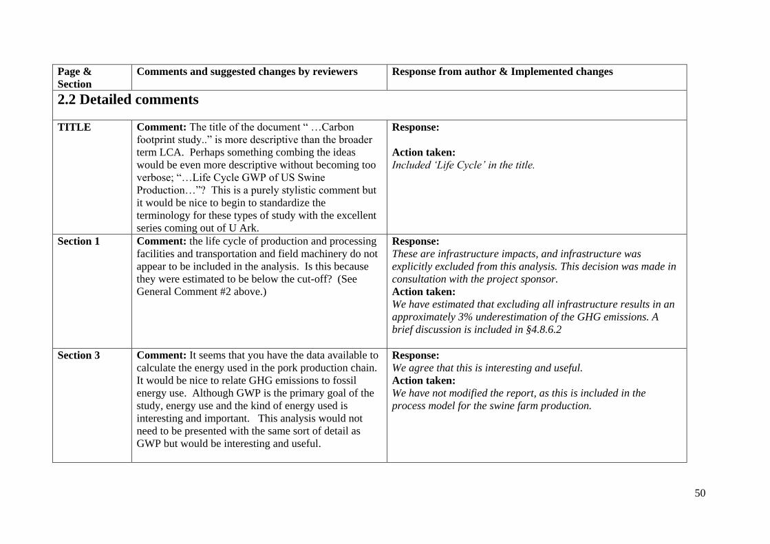
50

Page &

Section

Comments and suggested changes by reviewers Response from author & Implemented changes

2.2 Detailed comments

TITLE Comment: The title of the document “ …Carbon

footprint study..” is more descriptive than the broader

term LCA. Perhaps something combing the ideas

would be even more descriptive without becoming too

verbose; “…Life Cycle GWP of US Swine

Production…”? This is a purely stylistic comment but

it would be nice to begin to standardize the

terminology for these types of study with the excellent

series coming out of U Ark.

Response:

Action taken:

Included ‘Life Cycle’ in the title.

Section 1 Comment: the life cycle of production and processing

facilities and transportation and field machinery do not

appear to be included in the analysis. Is this because

they were estimated to be below the cut-off? (See

General Comment #2 above.)

Response:

These are infrastructure impacts, and infrastructure was

explicitly excluded from this analysis. This decision was made in

consultation with the project sponsor.

Action taken:

We have estimated that excluding all infrastructure results in an

approximately 3% underestimation of the GHG emissions. A

brief discussion is included in §4.8.6.2

Section 3 Comment: It seems that you have the data available to

calculate the energy used in the pork production chain.

It would be nice to relate GHG emissions to fossil

energy use. Although GWP is the primary goal of the

study, energy use and the kind of energy used is

interesting and important. This analysis would not

need to be presented with the same sort of detail as

GWP but would be interesting and useful.

Response:

We agree that this is interesting and useful.

Action taken:

We have not modified the report, as this is included in the

process model for the swine farm production.

51

Section 3.1.3

Figure 3

Comment: It would be helpful to see system

boundaries and all products/coproducts crossing these

boundaries (coproducts of abattoir and feed

processing). Also, the term “energy inputs” for, e.g.

pesticides, material inputs and refrigerants seems ill-

chosen. Consider using ISO nomenclature (reference

flows, intermediate flows, etc.).

Response:

Action taken:

We have modified the system diagram to show the broad classes

of co-products from the abattoir (figure 4) and feed processing

stages of the system which are primarily meat/bone meal and

tallow. These are used in a variety of downstream processes

which are outside the system boundary.

Section 3.1.3

Figure 3

Comment: “processing and transport” of crops has no

fossil fuel inputs and no GHG emissions?

Exports are shown but it is unclear how they are

handled: inventoried as U.S. consumption? Ignored?

Both of the comments in this box refer to the figure and

the associated text. Please be clear as to how these

were handled.

Response:

Explanation of exports was presented in §3.4. at the processing

plant gate, the difference between export and domestic pork is 2-

fold: different cut and different packaging. On a FU basis, the

export stream has no effect on the result; at the resolution of this

analysis, we did not have information specific to the impacts of

different cuts of meat, and packaging of exported meat is out of

the system boundary

Action taken:

The figure was updated to include inputs to processing and

transport. Additional discussion of export added to §3.4

Section 3.1.4 Comment: The functional unit definition is “prepared

for consumption” but this is not clearly defined. Later

(e.g., Section 4.2) there is discussion of different means

of cooking. Text also describes eight 4-ounce servings,

but it is unclear if they cut and then cooked, or cooked

as larger piece of meat and THEN cut?

Response:

We believe that the reviewers are concerned that the energy

requirements will be different depending on how the meat is

prepared, and agree that this is the case. However, this work is

not focused on the use phase, and the analysis of cooking options

is included primarily to illustrate that there are measurable and

significant emissions from this life cycle stage. Clearly

additional research and analysis is necessary to achieve the

resolution indicated by the comment.

Action taken:

For clarity, our assumption was that the meat was cooked and

then cut, and this has been included in the discussion (§ 3.6)

52

Section 3.1.5 Comment: It is stated that the ISO hierarchy was used,

and yet the preferred approach to deal with

multifunctional processes in this assessment is

economic allocation (third and final option in ISO) for

both feed processing by-products and rendering

products.

A mention that the actually chosen approach is the last

option according to the ISO hierarchy should be

included. A justification of why the preferred options

were not possible is also required.

Response:

Action taken:

Explanation added in §3.1.5

Section 3.1.6 Comment: A discussion on how biogenic carbon (in

CO2 and CH4) was dealt with is important in

agricultural product LCA. (Suggest referring to or

moving text from 3.3.3). Also, the justification for not

adjusting the biogenic CH4 characterization factor (to

account for initial uptake of CO2) should be given.

Response:

We are not clear why the reviewers believe an adjustment to the

methane GWP factor is needed. In the analysis published by the

IPCC the final degradation product of methane in the

atmosphere is carbon dioxide, which is persistent in the

atmosphere, and therefore a separate accounting of the

sequestration at crop growth would result in an under counting

of the GWP (that is the sequestered co2 ends back in the

atmosphere, just like for corn ethanol)

Action taken:

We have expanded the discussion in §2.3.3 to address biogenic

emissions more clearly.

Section 3.1.6 Comment: This section refers only to CO2, CH4 and

N2O, but introduction states inventory includes

refrigerants.

Response:

Refrigerants are mentioned in this section, and were included in

the analysis. The specific refrigerants used are available in the

model unit processes. It is not clear what action the review panel

expects based on this comment

Action taken:

None.

53

Section 3.2,

Figure 4

Comment: Replacement gilts are included in the

graphic, but these are not mentioned in the text, and do

not appear in the farm-gate GWP equation. They do,

however, appear in the model to which the critical

review team had access.

Response:

Action taken:

Added explanation that the inputs in the equation include the

replacement gilts, as modelled in the simapro model that was

reviewed.

Section 3.3 Comment: It is stated “A previously conducted

literature review is used as the basis for much of the

life cycle inventory data”. Please cite and, if helpful,

make available.

Response:

Action taken:

Citation added. This document should be available on the NPB

website.

Section 3.3.1 Comment: It is stated “we have identified the most

common feeds”. Is what is being considered in the

study an estimation of most common feeds, or an actual

production-weighted average? If an estimation of most

common feeds, then a measure of variability should be

included in subsequent uncertainty calculations.

Response:

The rations used in the model are estimated from swine nutrition

and typical growth rates. We have included effects of change in

the diet associated with replacement of ddgs with corn and soy.

Adding a PDF to the feed consumed without also changing the

live weight production is similar to changing the feed conversion

ratio; which confounds the results (that is the uncertainty in

variability of the ration is potentially amplified when the animal

weight is not also varied. Thus we have not added this analysis,

but have indicated in the discussion that the uncertainty ranges

are not fully reflective of the interdependent mechanisms due to

the fact that this is not a dynamic model.

The difference in the diet with and without DDG can be taken as

an expected range of variation of the ration composition

Action taken:

We have added references to typical swine diets.

54

Section 3.3.1.1 Comment: “Input data for fuels and electricity

consumption for crop production were obtained from

the technical literature, state agricultural extension

services, the US Department of Energy, the USDA, and

other academic institutions”: Please cite.

Response:

Action taken:

Citations added.

Section 3.3.1.1 Comments: “The EcoInvent database was used to

provide upstream information (i.e., production of

fertilizer)”: However, a review of the actual SimaPro

model reveals that the ecoinvent database was used for

more than only fertilizer production. Suggest replacing

“i.e.” with “e.g.”.

Response:

Action taken:

Corrected and clarified.

Section 3.3.1.1 Comments: “Industry estimates” often cited. Please

provide some details on how “industry estimates” were

derived (interviews? With whom? Actual data

collection templates or ad hoc telephone

conversations?)

Response:

Action taken:

Explanatory text added (e.g., §3.4) NDA in place for this project

prevent disclosure of the specific companies that provided data.

Section 3.3.1.1 Comments: It is not clear how the accounting was

done for distillers grains. All of the drying energy is

allocated to DDG. It seems that 98.6% of all other

inputs were allocated to ethanol, leaving 1.4%

allocated to DDG. Does this represent the economic

value of the DDG v. ethanol? If economic allocation

was used, provide justification for its use. Text is

ambiguous. Please clarify.

Response:

The unit process for DDG was adapted directly from the multi

output process, for US conditions, available from ecoinvent. The

only modifications made were to create a new unit process for

wet DDGs by removing the natural gas used for drying the DDGs

(system separation per ISO). The majority of the remaining

emissions were allocated economically by the EcoInvent center,

and this was directly adopted for this scan level work.

Action taken:

Section 3.3.1.2 Comments: Is footnote in first sentence of section

correct? The IPCC N2O emissions factors are found in

Chapter 10 which covers livestock and manure

management?

Response:

Chapter 11 covers field emissions and crop residues

Action taken:

The citation should be to chapter 11 of volume 4; corrected.

55

Section 3.3.1.2 Comments: Given the importance of the N2O

emissions and the uncertainly associated with the 1%

estimate, please report how the variability of this input

was handled in the sensitivity analysis. Variability due

N2O, as seen in SimaPro model, seems very small.

Response:

Agreed.

Action taken:

We have modified the geometric standard deviation for the

parameter N2O_residue which is used to convert N application to

N2O emissions. Based on the ranges for direct and indirect N2O

emissions, we defined the GSD so that the maximum emission

rate estimated (in which scenario only 40% of applied N is

available for plant growth, which on a national scale represents

extremely poor N management) fell at the 99th

percentile of the

associated distribution. The revised report includes this

additional uncertainty in the MCS and reported confidence

ranges.

Section 3.3.1.3 Comments: It is assumed that distiller‟s grains are

used in all rations (although different amounts are

considered). Is it the case that all or most swine are fed

DDGs, and if so is there a reference to support it? Do

you have data regarding what proportion of swine are

fed DDGs?

Response:

DDGS use in the swine industry is a moving target. As more

corn is converted to ethanol, DDGS production will increase and

so will it's use in swine diets. Use is dictated by the farms

relative location to an ethanol plant and cost of DDGS relative to

corn. Subsequently not all producers have access to DDGS. To

account for this, estimates of the carbon footprint were

calculated for both scenarios.

Action taken:

Section 3.3.1.3 Comments: “30 finished pigs plus one sow”: we

calculate 3.5x9.5=33.25 pigs. Perhaps one is used as

“sow replacement” (replacement gilts), but we still

have 32.25 pigs, not 30. Please explain the

discrepancy.

Response:

Action taken:

The figure ‘30’ corrected to the actual value used in the simapro

model of 32.25

56

Section 3.3.1.3 Comments: Some confusion exists around the

mortality of sows. If sows are expected to produce 3.5

parities at 9.5 piglets/parity, then shouldn‟t the

percentage sow mortality per (number of parities *

piglets per parity) be 100% ? It is much lower in

model.

Response:

Mortality refers only to those sows that are not sent to market,

but whose carcass is disposed.

Action taken:

Additional explanation added in the text in §4.2

Tables 1-4 Comments: Unit expressing feed rate is missing a unit:

Est. feed, lb/sow per how much time? For Table 3-4, a

“per life” figure is conceivable (about 2.8 lb ingested/lb

gained). For sows (Tables 1 and 2), one would need to

know if these values are for the average 3.5 parities

Response:

Action taken:

Heading was updated to clarify.

Section 3.3.2 Comments: Re. different manure management

systems, the text indicates that “Each can be modeled

separately.” It would be more useful to indicate what

was actually done in the study at this point. A review

of the model indicates that each was indeed modelled

separately.

Response:

Each system has a separate unit process in the model, and thus

different scenarios with single systems can be simulated. For the

national scale analysis, all of the management systems were

included in proportion to the fraction of manure managed, by

region (see Table 6).

Action taken:

We have added clarification to the discussion in this section

.

Section 3.3.2 Comments: The manure management of the “sow

barn” accounts for manure from sows but not from

piglets. How is this handled? Model and report are not

clear.

Response:

The ASABE reference indicates that the sow manure estimate

includes piglet manure.

Action taken:

Better documentation added to both.

Section 3.3.2.1

p. 13

Comments: Something seems wrong with the first

sentence …EF use the emissions in kilograms

…Should it perhaps be …EF is the emissions in

kilograms…

Response:

Action taken:

Corrected.

57

Section 3.3.3 Comments: The last sentence in this section is not

strictly correct. While methane is a more potent GHG,

it degrades in the atmosphere to less potent gasses

(~CO2). The 25 factor is the 100 year cumulative

GWP of methane as it is released (with a much higher

multiplier) and as it degrades into less potent GHGs.

Clarify assumption regarding plant fixation of CO2

versus release as methane and subsequent degradation

into CO2. (Also, see comment above on Section 3.1.6).

Response:

Action taken:

This was revised to clarify the role of biogenic methane.

Section 3.4.2

(and Section

4.5.2)

Comments: A log normal distribution is a very flexible

and useful, but is only appropriate when the variable is

restricted to positive values or the result of the

multiplication of two normally distributed variables. Is

this the case for all variables included in the Monte

Carlo analysis? Clarify which distributions were used,

what parameters were chosen, and how parameters

were chosen.

Response:

All of the material and energy flows in this model are positive-

definite, and therefore we judged that log-normal distributions

were most appropriate.

Action taken:

Section 3.4.2

and Section

4.5.2

Comments: A table that presents contribution and

sensitivity results side-by-side is recommended to

provide an overview of parameters contributing to

overall uncertainty. Are the numbers in Tables 9 and 12

representative of the variability‟s assigned for the

Monte Carlo simulation?

Response:

Action taken:

We have modified most of the figures in the report to make clear

which processes are contributing to the GHG emissions. The

values in the tables are representative of the distributions used in

the model. Some sensitivity analysis was restricted to evaluate,

comparatively, the impacts of different variables.

Section 3.4.3.1 Comments: Were the state production volumes (Table

6) used properly to allocate production to each

interconnect region? From where were the data on

electricity production (cradle-to-plug) taken? From a

review of the Simapro model, it appears only Eastern

Response:

As the reviewers indicate, electricity is a relatively minor

contributor to the footprint, and for consistency we modified the

model to use the national average electricity mix.

58

electricity was used for all life cycle stages (Western

set at 0, Texan not considered). Please address.

Also, the regionalisation of electricity data was only

done for foreground processes, i.e. the background

ecoinvent processes all use default (i.e. mostly

European) electricity. This should be clear in the

report. Note that the reviewers are conscious that the

impacts of this electricity use are minor and changing

this aspect of the model would probably not change the

outcome of the study.

Action taken:

Interconnect data replaced with national average primary energy

mix for electricity production. The report has been modified to

indicate this and to mention the reliance on background EU

processes.

Section 3.4.3.2 Comments: Provide source for both combustion and

pre-combustion emissions.

Response:

This language was intended to be explanatory of the processes

included by default in the Ecoinvent datasets for fuels consumed

in industrial settings. We did not in fact, in the model, separate

precombustion from combustion emissions.

Action taken:

We have re written this section to avoid the confusion introduced

by separation of life cycle phases of the fuel.

Section 3.4.3.3 Comments: What unit processes were used to

represent transport, and was the load factor adapted?

Response:

We did not adapt the load factor. We used a combination of

EUR3 transport and fleet average transport from the Ecoinvent

database.

Action taken:

None.

Section 3.4.3.4 Comments: Provide information in the report on data

sources for packaging (reference flows and inventory

data).

Response:

Action taken:

Added

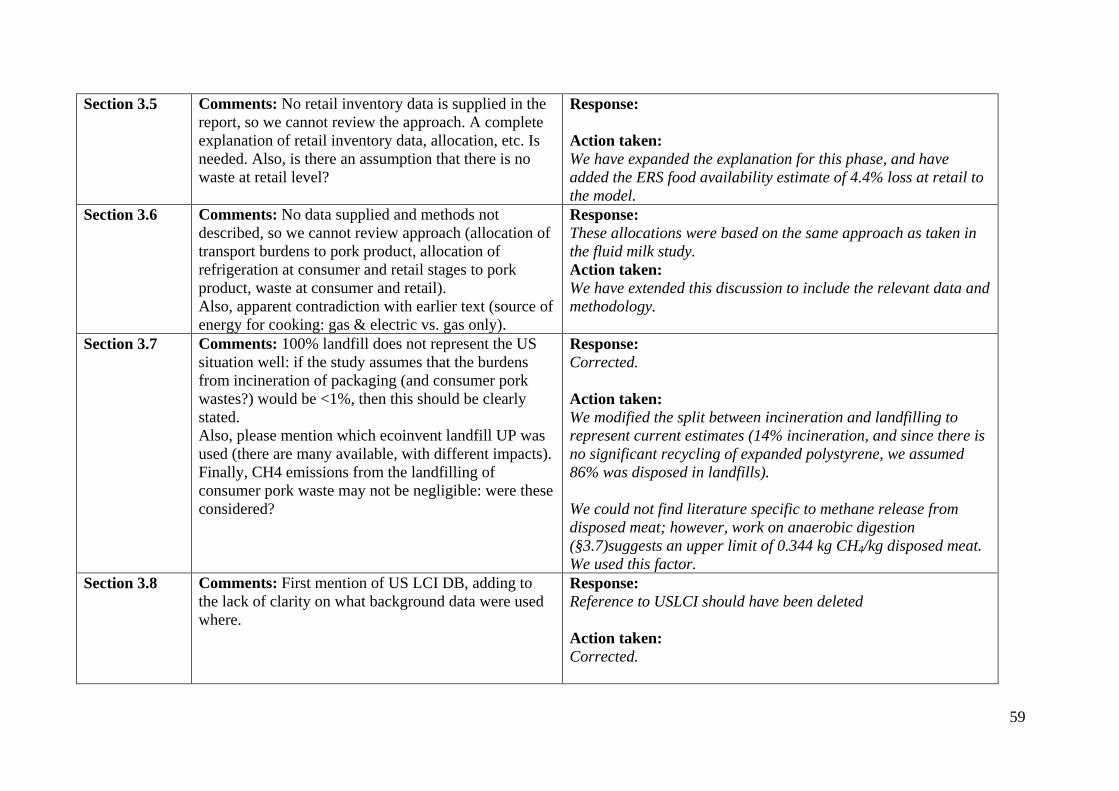
59

Section 3.5 Comments: No retail inventory data is supplied in the

report, so we cannot review the approach. A complete

explanation of retail inventory data, allocation, etc. Is

needed. Also, is there an assumption that there is no

waste at retail level?

Response:

Action taken:

We have expanded the explanation for this phase, and have

added the ERS food availability estimate of 4.4% loss at retail to

the model.

Section 3.6 Comments: No data supplied and methods not

described, so we cannot review approach (allocation of

transport burdens to pork product, allocation of

refrigeration at consumer and retail stages to pork

product, waste at consumer and retail).

Also, apparent contradiction with earlier text (source of

energy for cooking: gas & electric vs. gas only).

Response:

These allocations were based on the same approach as taken in

the fluid milk study.

Action taken:

We have extended this discussion to include the relevant data and

methodology.

Section 3.7 Comments: 100% landfill does not represent the US

situation well: if the study assumes that the burdens

from incineration of packaging (and consumer pork

wastes?) would be <1%, then this should be clearly

stated.

Also, please mention which ecoinvent landfill UP was

used (there are many available, with different impacts).

Finally, CH4 emissions from the landfilling of

consumer pork waste may not be negligible: were these

considered?

Response:

Corrected.

Action taken:

We modified the split between incineration and landfilling to

represent current estimates (14% incineration, and since there is

no significant recycling of expanded polystyrene, we assumed

86% was disposed in landfills).

We could not find literature specific to methane release from

disposed meat; however, work on anaerobic digestion

(§3.7)suggests an upper limit of 0.344 kg CH4/kg disposed meat.

We used this factor.

Section 3.8 Comments: First mention of US LCI DB, adding to

the lack of clarity on what background data were used

where.

Response:

Reference to USLCI should have been deleted

Action taken:

Corrected.

60

Section 3.8 Comments: Since readers will not have access to the

computational model, the citations would be better

placed in the actual report.

Response:

The majority of these are available in the literature review.

Action taken:

Added citation to literature review

It is confusing and inconsistent that the reader must do

a division to obtain the results per the stated functional

unit. If the functional unit is not actually used in the

study, why not use kg CO2eq/kg boneless pork

instead?

Response:

Agreed.

Action taken:

Except for gate-to-gate sections of the report (e.g., live weight at

farm gate) we have changed to functional unit basis with

parenthetical units in SI

Section 4 Comments: The SimaPro model refers to sows in

farrow/wean farms. These are not mentioned in the

report, or at least not under this name. Are these the

“Breeding/Gestation/Lactation” farms (also referred to

as sow barn?) of Chapter 4 of the report or

Nursery/Finish farms? Consistent nomenclature should

be used throughout report and models.

Response:

Farrow/wean actually refers to a barn, not a farm. It is the same

as breeding/gestation/lactation barn.

Action taken:

We have modified the terminology to be consistent across the

model and report.

Section 4.2 Comments: Review paragraph for clarity: “The overall

cumulative GHG emissions for consumption of one 4-

oz serving of US domestic pork using based on

reported manure management practices and accounting

for an estimated 10% waste of product by consumers

2.25 lb CO2e.. This model assumes gas oven cooking

in the home; if in-home cooking is assumed an electric

oven, the overall impact increases to 2.31 kg CO2e per

4oz serving. increases to 0.195 kg CO2e. In this

analysis, we have not accounted for any weight loss on

cooking. .” Also, note the mix-up in units (should say

2.31 lb CO2e, not kg).

Response:

Thank you.

Action taken:

Corrected §4.2

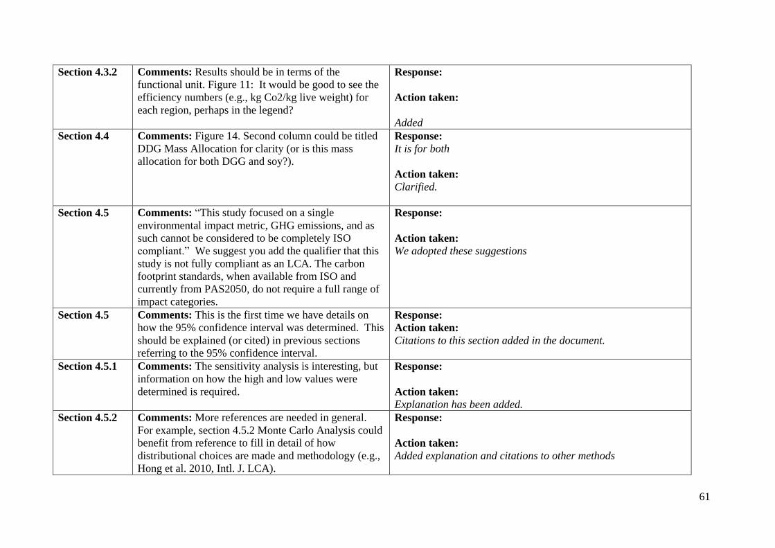
61

Section 4.3.2

Comments: Results should be in terms of the

functional unit. Figure 11: It would be good to see the

efficiency numbers (e.g., kg Co2/kg live weight) for

each region, perhaps in the legend?

Response:

Action taken:

Added

Section 4.4

Comments: Figure 14. Second column could be titled

DDG Mass Allocation for clarity (or is this mass

allocation for both DGG and soy?).

Response:

It is for both

Action taken:

Clarified.

Section 4.5 Comments: “This study focused on a single

environmental impact metric, GHG emissions, and as

such cannot be considered to be completely ISO

compliant.” We suggest you add the qualifier that this

study is not fully compliant as an LCA. The carbon

footprint standards, when available from ISO and

currently from PAS2050, do not require a full range of

impact categories.

Response:

Action taken:

We adopted these suggestions

Section 4.5 Comments: This is the first time we have details on

how the 95% confidence interval was determined. This

should be explained (or cited) in previous sections

referring to the 95% confidence interval.

Response:

Action taken:

Citations to this section added in the document.

Section 4.5.1 Comments: The sensitivity analysis is interesting, but

information on how the high and low values were

determined is required.

Response:

Action taken:

Explanation has been added.

Section 4.5.2

Comments: More references are needed in general.

For example, section 4.5.2 Monte Carlo Analysis could

benefit from reference to fill in detail of how

distributional choices are made and methodology (e.g.,

Hong et al. 2010, Intl. J. LCA).

Response:

Action taken:

Added explanation and citations to other methods

62

Section 4.5.2 Comments: The 95% confidence interval is based on

the use of lognormal distributions in Monte Carlo

(again, were they all lognormal?), but the choice of the

mean and variance of the underlying distributions were

chosen how? The confidence interval reported is based

on the assumption that the distributions accurately

represent reality AND that no other important variables

that are uncertain exist. More discussion and

qualifications are necessary. The 95% confidence

applies to the distribution as defined – and does not

include uncertainty in the estimation of the

distributional parameters.

The attribution of uncertainty factors is not consistent.

Most are based on the pedigree matrix, but some

appear baseless (e.g. for refrigeration) and others are

simply missing (when “calculations” are used in

SimaPro, which would require authors to enter

parameters in the equation in the parameter page and

enter the uncertainty on each parameter individually).

More importantly, the so-called "basic uncertainty" (or

intrinsic variability) factors used in the model do not

appear to reflect real-life variability of parameters.

Although the actual results of the LCA are not affected

by this, the uncertainty is (probably very importantly)

underestimated

Response:

Some of the Ecoinvent datasets have uniform or normal

distributions, but all distributions created for this project were

log normal. The mean was taken as the best estimate we could

find from the literature or from data provided specifically for this

project from NPB or stakeholders. The industrial data is covered

by non-disclosure agreement that does not allow release of the

participating company names.

We agree that the uncertainty analysis is not fully complete –

there may be variables that we have not included that are

important; however, we have made every effort to create a

complete model, subject to the cut-off criteria specified in the

goal and scope.

Action taken:

We have checked uncertainty attribution and added pedigree

matrix where relevant. We have added discussion of the

limitations of the uncertainty ranges reported due to the use of

parameters in the calculations in the report.

Without additional feedback, it is difficult to address the concern

that ‘basic uncertainty’ factors do not reflect actual variability.

All of the concerns raised in this context point to a lower than

actual range for the 95% confidence band, and we have indicated

this in the report; with regard to N2O, specifically, we have

increased the variance of the distribution significantly, and the

current CI include this effect.

Tables 10, 11 Comments: Include full units. Response:

Most of table 10 is dimensionless

Action taken:

Units added.

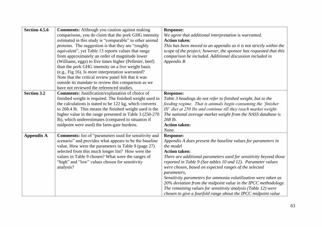
63

Section 4.5.6

Comments: Although you caution against making

comparisons, you do claim that the pork GHG intensity

estimated in this study is “comparable” to other animal

proteins. The suggestion is that they are “roughly

equivalent”, yet Table 13 reports values that range

from approximately an order of magnitude lower

(Williams, eggs) to five times higher (Pelletier, beef)

than the pork GHG intensity on a live weight basis

(e.g., Fig 16). Is more interpretation warranted?

Note that the critical review panel felt that it was

outside its mandate to review this comparison as we

have not reviewed the referenced studies.

Response:

We agree that additional interpretation is warranted.

Action taken:

This has been moved to an appendix as it is not strictly within the

scope of the project; however, the sponsor has requested that this

comparison be included. Additional discussion included in

Appendix B

Section 3.2 Comments: Justification/explanation of choice of

finished weight is required. The finished weight used in

the calculations is stated to be 122 kg, which converts

to 268.4 lb. This means the finished weight used is the

higher value in the range presented in Table 3 (250-270

lb), which underestimates (compared to situation if

midpoint were used) the farm-gate burdens.

Response:

Table 3 headings do not refer to finished weight, but to the

feeding regime. That is animals begin consuming the ‘finisher

III’ diet at 250 lbs and continue till they reach market weight.

The national average market weight from the NASS database is

268 lb.

Action taken:

None.

Appendix A Comments: list of “parameters used for sensitivity and

scenario” and provides what appears to be the baseline

value. How were the parameters in Table 9 (page 27)

selected from this much longer list? How were the

values in Table 9 chosen? What were the ranges of

“high” and “low” values chosen for sensitivity

analysis?

Response:

Appendix A does present the baseline values for parameters in

the model

Action taken:

There are additional parameters used for sensitivity beyond those

reported in Table 9 (See tables 10 and 12). Parameter values

were chosen, based on expected ranges of the selected

parameters,

Sensitivity parameters for ammonia volatilization were taken as

20% deviation from the midpoint value in the IPCC methodology.

The remaining values for sensitivity analysis (Table 12) were

chosen to give a fourfold range about the IPCC midpoint value

64

Second Round Critical Review Life Cycle Greenhouse Gas Emissions Baseline Study for the U.S. Pork Industry

Comments and suggested changes by reviewers Response from author & Implemented changes

Title Consider changing „Swine‟ to “Pork”. Pork is the

functional unit and most of the discussion uses the term

Pork rather than Swine. Per the functional unit, the report

addresses the production of pork – the flesh of a pig used

as food – rather than the animal. The report conclusion

section (§ 5) uses the word “pork” exclusively.

Response:

Action taken:

We have made this replacement.

Additional General

Comment

Upon reviewing the revised report the panel came to

recognize that the subject of this study is the full dressed

carcass. This fact is implicit in Figure 2 as well as Table

7 that shows that the animal is divided into two

categories: (1) meat; and (2) rendering and meat

byproduct. However, it is not explicitly stated in the

report that the subject is undifferntiated pork meat.

Although the functional unit is “one 4 ounce serving of

boneless pork”, the only explicit mention of a specific

type of pork meat product is the “2 pound tenderloin”

mentioned as an example of meat preparation by the

consumer. As this is among the more valuable cuts,

economic allocation using more disaggregated data

would have yielded a higher impact for tenderloin than

for generic, average meat. The approach taken is

appropriate for a scan study of this type, but a statement

should be included in § 2.1.3 that makes it clear that the

study does not differentiate between different types of

pork meat and that there is no attempt to account for

inputs to processed pork products such as bacon,

Response:

Action taken:

We have added this caveat to both section §2.1.2

(functional unit), and included more discussion in the

interpretation section of the report.

Regarding the variable allocation factor. The report

simply states that fixed allocation factors were used,

not that they could not be included in a Monte Carlo

analysis. The allocation for distillers grains was

calculated outside of SimaPro because individual line

items (natural gas for drying) have different allocation

factors, and SimaPro only allows a single allocation

factor between coproducts for all of the activity flows

in that unit process. Thus in a specific instance a

Monte Carlo simulation is not possible without also

manually manipulating an external spreadsheet for

each run of the Monte Carlo simulation.

With regard to the question about “sensitivity and

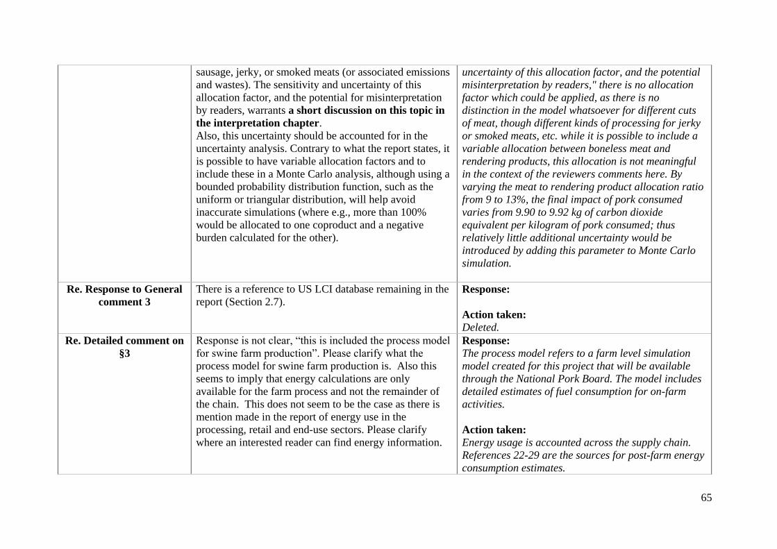
65

sausage, jerky, or smoked meats (or associated emissions

and wastes). The sensitivity and uncertainty of this

allocation factor, and the potential for misinterpretation

by readers, warrants a short discussion on this topic in

the interpretation chapter.

Also, this uncertainty should be accounted for in the

uncertainty analysis. Contrary to what the report states, it

is possible to have variable allocation factors and to

include these in a Monte Carlo analysis, although using a

bounded probability distribution function, such as the

uniform or triangular distribution, will help avoid

inaccurate simulations (where e.g., more than 100%

would be allocated to one coproduct and a negative

burden calculated for the other).

uncertainty of this allocation factor, and the potential

misinterpretation by readers," there is no allocation

factor which could be applied, as there is no

distinction in the model whatsoever for different cuts

of meat, though different kinds of processing for jerky

or smoked meats, etc. while it is possible to include a

variable allocation between boneless meat and

rendering products, this allocation is not meaningful

in the context of the reviewers comments here. By

varying the meat to rendering product allocation ratio

from 9 to 13%, the final impact of pork consumed

varies from 9.90 to 9.92 kg of carbon dioxide

equivalent per kilogram of pork consumed; thus

relatively little additional uncertainty would be

introduced by adding this parameter to Monte Carlo

simulation.

Re. Response to General

comment 3

There is a reference to US LCI database remaining in the

report (Section 2.7).

Response:

Action taken:

Deleted.

Re. Detailed comment on

§3

Response is not clear, “this is included the process model

for swine farm production”. Please clarify what the

process model for swine farm production is. Also this

seems to imply that energy calculations are only

available for the farm process and not the remainder of

the chain. This does not seem to be the case as there is

mention made in the report of energy use in the

processing, retail and end-use sectors. Please clarify

where an interested reader can find energy information.

Response:

The process model refers to a farm level simulation

model created for this project that will be available

through the National Pork Board. The model includes

detailed estimates of fuel consumption for on-farm

activities.

Action taken:

Energy usage is accounted across the supply chain.

References 22-29 are the sources for post-farm energy

consumption estimates.

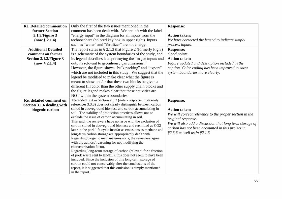
66

Re. Detailed comment on

former Section

3.1.3/Figure 3

(now § 2.1.4)

Only the first of the two issues mentioned in the

comment has been dealt with. We are left with the label

"energy input" in the diagram for all inputs from the

technosphere (colored key box in upper right). Inputs

such as “water” and “fertilizer” are not energy.

Response:

Action taken:

We have corrected the legend to indicate simply

process inputs.

Additional Detailed

comment on former

Section 3.1.3/Figure 3

(now § 2.1.4)

The report states in § 2.1.3 that Figure 2 (formerly Fig 3)

is a schematic of the system boundaries of the study, and

its legend describes it as portraying the “major inputs and

outputs relevant to greenhouse gas emissions.”

However, the figure shows “bulk packing” and “export”

which are not included in this study. We suggest that the

legend be modified to make clear what the figure is

meant to show and/or that these two blocks be given a

different fill color than the other supply chain blocks and

the figure legend makes clear that these activities are

NOT within the system boundaries.

Response:

Good points.

Action taken:

Figure updated and description included in the

caption. Color coding has been improved to show

system boundaries more clearly.

Re. detailed comment on

Section 3.1.6 dealing with

biogenic carbon

The added text in Section 2.3.3 (note - response mistakenly

references 3.3.3) does not clearly distinguish between carbon

stored in aboveground biomass and carbon accumulating in

soil. The stability of production practices allows one to

exclude the issue of carbon accumulating in soil.

This said, the reviewers have no issue with the exclusion of

carbon stored in aboveground biomass and reemitted as CO2

later in the pork life cycle insofar as emissions as methane and

long-term carbon storage are appropriately dealt with.

Regarding biogenic methane emissions, the reviewers agree

with the authors' reasoning for not modifying the

characterization factor.

Regarding long-term storage of carbon (relevant for a fraction

of pork waste sent to landfill), this does not seem to have been

included. Since the inclusion of this long-term storage of

carbon could not conceivably alter the conclusions of the

report, it is suggested that this omission is simply mentioned

in the report.

Response:

Action taken:

We will correct reference to the proper section in the

original response.

We will also add a discussion that long term storage of

carbon has not been accounted in this project in

§2.3.3 as well as in §2.1.3

67

Re. §3.3.1 The response is a bit unclear. Perhaps what you intended to

say is that there are not a big differences in swine diets by

region (e.g. compared to dairy?). Please clarify response.

Response:

Original comment: “It is stated “we have identified

the most common feeds”. Is what is being considered

in the study an estimation of most common feeds, or

an actual production-weighted average? If an

estimation of most common feeds, then a measure of

variability should be included in subsequent

uncertainty calculations.”

Action taken:

We used an estimated ration, not a production

weighted ration. This comment relates to the

composition of the ration which has an influence on

the time in the barn and final weight of the finished

animals. Because this LCA model is not structured to

include indirect, and linked effects, we have not

explicitly modelled the uncertainty associated with

variation in ration. However, as the final weight is a

stochastic variable in the MCS, a portion of this

variability is in fact captured in the simulations with

uncertain final animal weight.

Re. §3.3.1.3 Although DDG feeding to swine is a „moving target”, it seems

to be a very small moving target. I found reference to 1% and

11% of DDGs produced in the US fed to swine. The 1%

figure seemed to imply a national average while the 11%

seemed to imply an average in Iowa and MN where swine

facilities are in close proximity to Ethanol plants. We suggest

mention the fact that feeding DDGs to swine is done but

represents a small fraction of the nationally aggregated diet at

present, and that this percentage may increase in future.

Response:

Action taken:

We have incorporated these suggestions into the

document in § 3.3.

NEW COMMENTS:

§2.2

Figure 4: “9.5 weaned piglets per sow” should read

“33.25 weaned piglets per sow” (9.5 figure is “per

litter”).

Response:

Action taken:

Corrected

68

§2.6 Transport from retail to home is included: there should

be some description of how the impact of this transport,

where one can assume that often full groceries will be

transported, is allocated to pork.

Response:

Action taken:

We have included more detail in the discussion (§2.5

and §3.4)

§2.3 Reference to §4.8 is incorrect, should be to §4.2.5. Also,

please consistently refer to economic input output

data/databases as IO or EIO to minimize confusion.

Response:

Action taken:

Corrected.

§4 First sentence doesn‟t scan. Some words were dropped? The

intent seems to be to state that LCA requires multiple

performance metrics, while carbon footprint standards like

PAS 2050 do not. As currently written it doesn‟t make sense.

Response:

Action taken:

Rephrased

§4.2.3 The report states that "variables that have been parameterized

to allow sensitivity analysis do not have distributions assigned

as the Simapro software does not support this feature". There

is a quick work-around for this problem: one simply needs to

add the uncertainty to the parameters themselves, in the

"parameters" window. This is a simple process that we

estimate can be completed in approximately 30 minutes for the

parameters in question. It should be done and the Monte Carlo

re-run.

Response:

Action taken:

In fact, the majority of parameters for which a pdf is

relevant did have assigned values, and thus the effect

of uncertainty in parameter values is substantially

included.

§4.3 This section seems to be a straight cut and paste from a former

project. The milk project is discussed, the functional unit is

identified as a gallon of fluid milk consumed, and the wrong

audience is identified (general market, rather than the

"stakeholders in the swine industry value chain" mentioned in

§ 2.1.7).

Response:

Thanks.

Action taken:

Corrected.