NBER WORKING PAPER SERIES

DO SCHOOL SPENDING CUTS MATTER? EVIDENCE FROM THE GREAT RECESSION

C. Kirabo JacksonCora WiggerHeyu Xiong

Working Paper 24203http://www.nber.org/papers/w24203

NATIONAL BUREAU OF ECONOMIC RESEARCH1050 Massachusetts Avenue

Cambridge, MA 02138January 2018

The statements made and views expressed are solely the responsibility of the authors. Wigger andXiong are grateful for financial support from the US Department of Education, Institute of EducationSciences through its Multidisciplinary Program in Education Sciences (Grant Award # R305B140042).The views expressed herein are those of the author and do not necessarily reflect the views of the NationalBureau of Economic Research.

At least one co-author has disclosed a financial relationship of potential relevance for this research.Further information is available online at http://www.nber.org/papers/w24203.ack

NBER working papers are circulated for discussion and comment purposes. They have not been peer-reviewed or been subject to the review by the NBER Board of Directors that accompanies officialNBER publications.

© 2018 by C. Kirabo Jackson, Cora Wigger, and Heyu Xiong. All rights reserved. Short sections oftext, not to exceed two paragraphs, may be quoted without explicit permission provided that full credit,including © notice, is given to the source.

Do School Spending Cuts Matter? Evidence from The Great Recession C. Kirabo Jackson, Cora Wigger, and Heyu XiongNBER Working Paper No. 24203January 2018, Revised August 2019JEL No. H0,H61,I2,I20,J0

ABSTRACT

During The Great Recession, national public-school per-pupil spending fell by roughly seven percent,and took several years to recover. The impact of such large and sustained education funding cuts isnot well understood. To examine this, first, we document that the recessionary drop in spending coincidedwith the end of decades-long national growth in both test scores and college-going. Next, we showthat this stalled educational progress was particularly pronounced in states that experienced largerrecessionary budget cuts for plausibly exogenous reasons. To isolate budget cuts that were unrelatedto (a) other ill-effects of the recession or (b) endogenous state policies, we use states’ historical relianceon State taxes (which are more sensitive to the business cycle) to fund public schools interacted withthe timing of the recession as instruments for reductions in school spending. Cohorts exposed to thesespending cuts had lower test scores and lower college-going rates. The test score impacts were largerfor children in poor neighborhoods. Evidence suggests that both test scores and college-going weremore adversely affected for Black and White students than Latinx students.

C. Kirabo JacksonNorthwestern UniversitySchool of Education and Social Policy2040 Sheridan RoadEvanston, IL 60208and NBERkirabo-jackson@northwestern.edu

Cora WiggerNorthwestern University2120 Campus DriveEvanston IL 60208CoraWigger2021@u.northwestern.edu

Heyu XiongSchool of BusinessCase Western Reserve Universityheyuxiong2018@u.northwestern.edu

I IntroductionDuring The Great Recession, real pre-tax income fell by almost seven percent (Larrimore et al.

2015), national consumption as a percentage of GDP fell by 6 percentage points (Petev and Pista-ferri 2012), and property values fell by about 18 percent.1 Public schools are largely funded by acombination of property, income, and sales taxes. As such, public-school per-pupil spending fellby roughly seven percent nationally, by over ten percent in 7 states, and more than twenty percentin 2 states (Leachman et al. 2017). While per-pupil spending growth slowed during previous reces-sions, the Great Recession represents the largest and most sustained decline in national per-pupilspending in over a century (NCES 2017; Jackson et al. 2014).2 While compelling recent evidencebased on localized quasi-experimental variation indicates that increased school spending typicallyimproves child outcomes (Jackson 2018a), the sheer magnitude of this historical episode allowsfor a unique examination of the extent to which large-scale and persistent education budget cutsmay harm students in general, and poor children in particular. In this paper, we exploit plausiblyexogenous reductions in public school spending induced by the Great Recession and examine theeffect of school spending cuts on student test scores, and college-going rates.

We document that, nationally, the decline in school spending beginning with the onset of therecession is associated with the first time that average national test scores declined (in both mathand reading) in the past 50 years (Figure 1). The stalled progress in the National Assessment ofEducational Progress (NAEP) after 2009 has been documented by education scholars (e.g. West2018, Loeb 2018) and has been dubbed the “Lost Decade” in educational progress (Petrilli, 2018).The timing of the recessionary spending cuts also coincides slower growth in the number of first-time college entrants in the united states (Figure 1). A “naive” estimate based on the coincident timetrends, is that a $1,000 reduction in per-pupil spending (about an 8.3 % increase) was associatedwith an 8.7 percent of a standard deviation reduction in test scores and a 13.7 percent reduction inthe number of first-time college entrants. While these patterns are suggestive, one must interpretcoincident national trends with caution (Jackson et al., 2015). Because many other things mayhave changed nationally after the recession that could drive these associations, these relationshipsmay not be causal.3 To address these concerns and to isolate the impact of recession-induced schoolspending cuts from the broader impacts of the recession itself, we propose an instrumental variablesapproach that uses plausibly exogenous state-level variation in public K12 school spending.

1This is based on the Case-Shiller Index at the start and end of the recession. Note that housing prices has been onthe decline before the onset of the Great Recession, so that this does not reflect the full peak to trough decline.

2Indeed, as of 2016, 25 states had not recovered to their inflation adjusted per-pupil spending levels, and by 2019(more than a decade later) 12 states spent below their 2007 levels (link).

3In related work, Shores and Steinberg (2017) find that school districts in locations that were hardest hit by therecession had larger test score reductions when these districts hired fewer teachers and spent less on schools. However,they do not isolate the impact of school spending from that of other impacts of the recession.

1

Our identification strategy relies on the fact that states that were more reliant on state-collectedrevenues to fund public education (due to the particulars of their funding formulas) tended to ex-perience larger school-spending reductions during the recession. This is for two distinct reasons:First, during the Great Recession, as payments increased for Medicaid and Unemployment Insur-ance, states allocated a smaller share of their budgets to K12 education – a crowd-out effect. Thisreduction is illustrated in the left panel of Figure 2. Second, state-collected revenues are based ontax bases that are more responsive to market fluctuations than are local or federal revenues (Sobeland Wagner; Evans et al. 2017) – a revenue effect. For both these reasons, while overall schoolspending declined after recession onset, revenues from state taxes fell the most sharply (right panelof Figure 2). In Section III, we discuss why this was true even though the Great Recession was asso-ciated with declining house prices. We show that a state’s reliance on state revenues to fund publiceducation is highly predictive of reductions in per-pupil spending after the recession. Exploitingthis pattern, we instrument for per-pupil spending with the share of a state’s public school revenuesthat came from state sources before the recession interacted with the timing of the recession.

Our strategy requires that states with different reliance on state revenues were not differentiallyaffected by the recession for reasons other than through school spending. We show that this is likelyto be true in a few ways. First, our instrument predicts overall school spending primarily throughits predictable impact on state revenues (as opposed to local or federal revenues). Also, conditionalon ex-ante predictors of recession intensity, instrumented school spending is unrelated to measuresof economic conditions such as unemployment or poverty rates. Finally, our main results persist inmodels that control for contemporaneous local economic conditions and even house prices directly.

Our first main outcome of interest is student test scores from the National Assessment of Educa-tional Progress (NAEP). Our other main outcome is college-going obtained from the the IntegratedPostsecondary Education Data System (IPEDS). We link these outcome data to state-level spendingdata from the Census F33 School District Finance Survey (CCD) and our instruments for publicschool K12 spending. Our final dataset straddles the recession and includes data between years2002 and 2017. We proxy for a state’s vulnerability to recessionary budget cuts using its relianceon state revenues to fund public K12 schools in 2008. Relative to each state’s own time trend, wedocument a robust monotonic relationship between greater reliance on state funds in 2008 and theannual decline in per-pupil spending after the onset of the Great Recession. The pattern of greaterdeteriorating outcomes after the recession for states that are more reliant on state revenues is mir-rored for both test scores and college-going rates. These declines in test scores and college-goingtrack the recession-induced decline in per-pupil spending, and do not abate as the economy re-covered – evidence that these impacts are driven by the spending changes rather than other effectsof the recession per se. Using these patterns in an instrumental variables approach, on average, a$1000 reduction in per-pupil spending led to about 0.045 standard deviations lower test scores (p-

2

value<0.01) and between a 2.6 and 6.2 percentage points lower college-going rate (p-value<0.05).

We test for heterogeneous effects in a few ways. First, we use the individual-level NAEP tocompute the relationship between the district poverty rate and NAEP scores in each state in eachyear (following Card and Payne 2002 and Lafortune et al. 2018). We then estimate the impact ofrecession-induced spending changes on this slope. We find a consistent positive impact of spendingon this slope – indicating that test scores in high-poverty areas were more adversely effected by thespending cuts than in low-poverty areas. We also examine impacts by student race. In general, themarginal impacts are similar for Black and White students. However, impacts are larger for Blackand White students than for Hispanic students. We also explore heterogeneity in the college-goingeffect by institution type. We find increases at both 2-year and 4-year colleges. The 4-year collegeeffects are concentrated at non-selective institutions and those with more part-time than full-timestudents. We also find large increases at minority serving institutions (particularly those servingBlack students)– a pattern consistent with our test-score impacts by race.

To explore mechanisms, we examine what kinds of spending categories were most affected.In general, states cut spending across a broad range of categories. States that cut spending (aspredicted by our instruments) hired fewer teachers, fewer aides, and fewer library staff. However,states responded to spending cuts by disproportionately cutting more from construction expendi-tures and less from core K12 spending. While construction spending makes up 6.9 percent ofthe average school’s budget, it accounted for between 31 and 48 percent of the reduced spending.These patterns differ from those documented for spending increases due to school finance reforms(Jackson et al., 2016), suggesting that the marginal propensity to spend on different inputs may varywhen there are spending increases versus decreases. This may reflect districts attempting to shieldcore operational spending (to some extent) or districts being more constrained in their ability (ordesire) to cut spending on core school operations.4 To determine whether the impact of these largerecessionary spending cuts differ from those found in other studies (based largely on school spend-ing increases and localized quasi-random variation) we summarize the studies outlined in Jackson(2018b).5 Our estimated impacts are near the median effect across quasi-experimental studies thatexamine the impacts of spending (not tied to specific uses) on test scores – suggesting that themarginal effects of education spending cuts are largely symmetric to those of spending increasesdocumented in other settings.

Our results shed some light on how the changing structure of school finance may have madestudent achievement more sensitive to the business cycle. While state taxes account for about

4These different marginal propensities to spending categories could have lead to asymmetric spending impacts ifthe marginal benefit of construction spending differed markedly from that of other kinds of spending. However, asdocumented in Jackson (2018a) construction spending does, at times, affect student outcomes so that this reallocationof budgets may not have changed the marginal impact of school spending (relative to that for a spending increase).

5We are deeply grateful to Claire Mackevicius for coding the studies and running the formal meta-analysis.

3

half of all public school spending, this was not always so. Prior to the 1970s, school districts inthe United States funded public schools mostly through locally raised property taxes (Howell andMiller 1997; Hoxby). As such, poor districts tended to spend less per pupil than wealthier districts.The school finance reform movement (starting in the 1970s) lead to increased state collected taxesto maintain a more equitable distribution of school spending across districts. Because state fundingis more vulnerable to recessionary cuts, one potential “side-effect” of the increased centralization ofschool funding (i.e. use of more state funding) is an increased vulnerability of education spendingand, therefore, student achievement to fluctuations in the business cycle. Our results show this tobe the case. Our results also suggest that this increased sensitivity may be most pronounced forhigh-poverty districts that rely more heavily on state aid.

Broadly, our findings contribute to long-standing debates around whether school spending mat-ters and whether schools make do with less by showing that spending cuts harm students. Ouranalysis contributes to the field of public finance by shedding light on how the revenue sourcesused to fund public schools may have implications for student achievement. Finally, our resultsdeepen our understanding of the long-run effects of growing up during a recession. While it iswell-documented that growing up during a recession can lead to long lasting ill-effects throughchannels such as parental job displacement (Oreopoulos et al. 2008; Ananat et al. 2011; Stevensand Schaller 2011) and increased food insecurity (Gundersen et al. 2011; Schanzenbach and Lau-ren 2017), we provide new compelling evidence that recessions have lasting ill-effects on youngindividuals through their effects on the governments’ abilities to provide public education services.

The remainder of the paper is as follows. Section II describes the data. Section III describes theempirical strategy. Section IV presents the results. Section V concludes.

II DataWe link several data sources for our analysis.6 School finance data come from the Annual

Survey of School System Finances at the U.S. Census Bureau. The surveys contain financial datafor all public school districts in the United States (approximately 13,500). The financial surveysare available from 1987 through 2016. They provide education revenue broken down by source(local, state, and federal), and break down expenditures into broad categories. The share of schoolspending from each source varies substantially by state. Between 2002 and 2016, the average shareof school revenue from federal, state, and local sources were 9.5%, 48.7%, and 41.7%, respectively.While the share of federal revenue varies only between 4% (Connecticut and New Jersey) and 22%(Mississippi), variation in local and state revenue sources is much broader. The share of fundingthat comes from state sources varies between 0% (Washington, D.C.) and 90% (Hawaii). Theshare of revenue coming from state sources is central to our empirical strategy. We discuss in

6We provide more detail on our data sources in the Appendix.

4

detail how we use this variable to classify states in Section III. On average, 85% of public schoolspending goes to current elementary and secondary spending, which broadly includes expenses forinstruction and support services. Ten percent of public K12 education expenditures go towardscapital, which includes construction, land, and equipment. Salaries and benefits (instructional andnon-instructional) make up 68% of public school spending on average.

Test score data come from the NAEP. The NAEP is referred to as the Nation’s Report Card asit tests students across the country on the same assessments and has remained relatively stable overtime. The NAEP is administered every other year to a population-weighted sample of schools andstudents. For the main analyses, we use publicly-available state-year average scores.7 We focuson public school students’ 4th and 8th grade Math and Reading assessment scores. To facilitatecomparisons over time, we report NAEP scores standardized to a base year of 2003. The NAEPsample has been increasing over time and only stabilized after 2000 (Table A1). We focus on theperiod between 2002 and 2017.8 To conduct subsample analyses, we also utilize restricted-use datafiles with student-level scores and demographics. The individual-level NAEP dataset includes 4.3million individual NAEP scores from 11,477 school districts between 2002 and 2015.

Our college-going data are from the the IPEDS. These data report surveys submitted at theaggregate-level from postsecondary institutions. These data do not have student-level informa-tion. Institutions report on the number of first-time college freshman from each state in each year.By aggregating these data to the state of origin level, we obtain counts for the number of first-time freshmen from each state in each year. Using information on postsecondary institutions fromIPEDS and the Carnegie Foundation, we compute enrollments by college type (2-year vs 4-year)and selectivity level. To compute college-going rates for these years, we obtain population countsby age in each state in each year from the American Community Surveys (ACS) from 2000 to 2016.Our college-going measure is the number of first-time college enrollees divided by the number of17-year-olds in the state two years prior.

As additional variables, we obtain estimates on the total population, child population, and childpopulation living in poverty for the geographic areas associated with school districts from theUnited States Census Bureau Small Area Income and Poverty Estimates (SAIPE). We also usearea economic indicators of employment and wages from the Bureau of Labor Statistics (BLS)and an annual measure of home values in each state from Zillow. We also include public schooldistrict staffing and student enrollment information from the Common Core of Data LEA Universesurveys from the National Center for Education Statistics (NCES).9 Our state-year level dataset issummarized is summarized in Table 1.

7Obtained from http://apps.urban.org/features/naep/8Because the 2017 school spending data was not available at the time of our analysis, we use 2016 school spending

data for 2017 test scores.9When these data are missing, we impute with the mean. This does not affect the results.

5

III Empirical StrategyThe Great Recession led to a historic decline in per-pupil spending. As shown in Figure 1, the

decline in school spending during the recession coincides with the first average national test scoredecline (in both math and reading) in the past 50 years, and with a slowing in the number of first-time college entrants in the United States. While these coincident trends are highly suggestive, theymay not reflect causal relationships. As such, we seek to separate the effect of recession-inducedschool spending declines from that of the recession itself (and other potentially confounding policyor demographic changes). To this aim, we employ an instrumental variables approach. Our instru-mental variables strategy relies on the fact that states that were more reliant on states revenues tofund public K12 schools were more likely to experience declines in school spending for reasons un-related to the intensity of the recession in the state or other policy changes that may have occurredat that time. This basic pattern holds true for two related, but distinct reasons.

The first reason is that as the labor market worsened, demand for state-funded services such asunemployment insurance and Medicaid increased (Moffitt 2013). To cover these additional costs,many states cut their education budgets – resulting in a crowding out effect. This pattern is shownin the left panel of Figure V. Prior to the Great Recession, states spent about 27% of their budgetson K12 schools. However, after the Great Recession, this fell to about 23% and remained at thatlevel through 2015. This pattern is not unique to the Great Recession and can also be observed withthe early 2000s recession when the share of state spending going to K12 school fell from about 29%to about 27%. This suggests that, even even if state revenues were unchanged during the recession,states that were more reliant on state taxes to fund K12 schools would be more likely to experienceeducation budget cuts. We refer to this as the crowd-out channel.

The second reason that greater reliance on state revenues to fund public schools was associatedwith deeper education spending cuts has to do with the tax bases. Revenue sources used to collectstate taxes (mostly income and sales taxes) are more variable than revenues used to collect localtaxes (mostly property taxes). Estimates suggest that income and sales taxes have a short-runelasticity (with respect to the tax base) of over 1 (Holcombe and Sobel 1995). In contrast, propertytaxes (which comprise the lion’s share of local revenues) are more stable. Property tax revenueshave a short-run elasticity (with respect to home values) of only between 0 and 0.4 because (a) taxesare collected on assessed values which follow market value with a considerable lag (Lutz 2008),and (b) policy-makers often offset declines in assessed values with higher tax rates (McMillen2011; Lutz et al. 2010).10 The greater sensitivity of state taxes (as opposed to federal or local taxes)to the business cycle suggests that, even if there were no crowd-out channel, states that were morereliant on state taxes to fund K12 school would experience deeper education budget cuts (as shown

10Evans et al. (2017) show that revenues from property taxes actually grew for three years after recession onset.

6

in Chakrabarti et al. 2015; Leachman and Mai 2014). We refer to this as the revenue channel.

We define the parameter Ωs as the share of state K12 revenues in state s that came from statesources in 2008.11 Through both channels, Ωs is meant to capture vulnerability to recessionaryschool spending cuts.12 We classify states based on the source of the revenue as reported in AnnualSurvey of School System Finances at the Census Bureau. For almost all states, this classificationcaptures both channels outlined above. An example of a highly vulnerable state is Hawaii. In 2008,Hawaii received 85% of its education funding from the state (making it vulnerable to the crowd-outeffect), and 75% of its state revenues came from income or sales taxes (making a large share of itsrevenue sensitive to the business cycle).13 An example of a less vulnerable state is Illinois. In 2008,Illinois received 34% of its K12 spending from the state (making it less vulnerable to the crowd-out effect), and only 30% of its revenues come from income or sales taxes (making a relativelysmall share of its revenue sensitive to the business cycle). To further elucidate our instrument,we discuss a slightly less straightforward state – California. Due to California’s Proposition 98,the state collects some (but not all) locally raised property tax revenue that goes into the Stategeneral fund. From the centralization perspective, one may consider the locally raised taxes that arecollected by the state to be state revenue. However, because the Proposition 98 funding is typicallyearmarked specifically for education and cannot be borrowed from, it makes more sense to classifythese funds as local (i.e. less sensitive to the centralization channel). Also, from the revenuecyclicality perspective, these property taxes are less variable than income and sales taxes so thatone may wish to classify them as local taxes. For both these reasons, we follow the Census Bureaucategorization and classify these funds as local funds. Doing so, we classify 58% of California’seducation revenue as coming from state sources. Note that all of our results are robust to how weclassify these potentially ambiguous funds, and to dropping California from the sample.14

11Following Evans et al. (2017), we compute the share of K12 revenues in state s that came from state sources in2007-2008 (determined pre-recession) across all districts in the state as follows:

Ωs =∑d∈s StateRevenued

∑d∈s TotalRevenued

StateRevenued denotes the school revenue in district d which came from state sources in the 2007-2008 school year;and TotalRevenued is the total revenue collected in district d in the same year.

12Figure A3 shows that Ωs is evenly distributed across the geographic regions of the nation.13Information on revenue sources come from (Saito, 2008)14There is one ”state” for which classification is unclear, which is the District of Columbia (DC). In essence, DC is

not a state, so by definition does not have state taxes. Because DC serves as the federal capital, the constitution grantsthe United States Congress jurisdiction over the District. This is evidenced by the fact that the Federal governmentcovers about one-quarter of DC’s budget, and the fact that DC received large amounts of increased Federal fundsduring the recession. As such, from the centralization perspective, we follows the categorization employed by theCensus Bureau and classify municipality funds that support education as “local” and set state revenues equal to 0. Thissuggests that D.C. experiences little vulnerability to recessionary spending cuts due to our instrument. Based on Figure2, this categorization appears to hold empirically. Because this is a judgment call, we show that all of our results arerobust to dropping data from D.C. entirely.

7

Through both the crowd-out and revenue channels, while overall school spending declined afterrecession onset, revenues from state taxes fell most sharply (Figure 2). As such, states that weremore reliant on state revenues to fund public education in 2008 (due to the particulars of their schoolfunding formulas) tended to experience larger school spending reductions during the recession.Figure 3 plots the state-level percent change in per-pupil spending between 2007 and 2011 (pre-and post-recession) against the share of K12 spending in the state that came from state sources in2008. As one might expect, Figure 3 shows a clear tendency for states that were more reliant onstate sources prior to the recession to have larger reductions in K12 spending during the recession.The basic pattern of larger spending cuts in state that were more reliant on state revenues to fundpublic education motivates our instrumental variables approach. We use Ωs as an exogenous shifterof K12 spending within states during the recession. For our approach to uncover a school spendingeffect, Ωs should not be correlated with changes in other policies or economic conditions withinstates. We argue that a state’s reliance on state revenues to fund education prior to the recession isunrelated to the impact of the recession on other dimensions in that state. To asses this, the rightpanel of Figure 3 plots changes in the state unemployment rate between 2007 and 2011 by Ωs.While there was a general increase in unemployment in the average state, Ωs was unrelated to theimpact of the recession in that state. We present more formal tests below.

III.1 Estimation EquationOur empirical approach is to compare the change in outcomes before and after the recession

across states that were more or less reliant on state revenues (and therefore experienced larger orsmaller reductions in school spending). To rely only on within-state variation, we allow each stateto have its own intercept and linear time trend in both spending and in the outcomes.

In our first stage regressions, we show that relative to each state’s own pre-recession trend in

school spending states that were more reliant on state revenues to fund public education (in 2008),had a more negative post-recession time trend in school spending. If school spending affects out-comes, then in a reduced-form model, the change in the trend in school spending should correspondwith a change in the trend in test scores and college-going. We show that this is the case.

In Figure V, we present an event-study for the recession’s effect on K12 spending, averageNAEP scores, and college-going rates by states’ reliance on state revenue sources. We estimatemodels as below on our state-level panel for various outcomes Y for each state s in each year t, Yst .

Yst =2017

∑t=2002

βt · (Ig>1,s× IT=t)+ γs +(τs×T )+υst (1)

In 1, IT=t is an indicator denoting if the observation is for calendar year t and Ig=1,s denotes thestates that are more reliant on state revenues for public schools (that is, states that relied on state

8

revenues for more than one third of education spending in 2008). To account for differences acrossstates we include state fixed effects γs. To compare changes in each state’s outcome to its own timetrend, we include the state-specific linear time trends τs. The variable υst is a random error term.The coefficients βt map out the differences in outcomes between states with low and high Ωs ineach year (relative to each states own pre-recession intercept and linear time trend). We estimatethis model by OLS on per-pupil spending (in 2015 dollars), average state-level NEAP scores, andcollege-going rates. We plot these coefficients along with the 95% confidence interval for eachcoefficient estimate in Figure 4 where the reference year is 2007.

The event study for test scores are in the top left panel. Prior to the recession, school spendingwas on a similar trajectory in areas with different levels of Ωs, but after the recession, states withheavy reliance on state revenues experienced a clear linear decline in per-pupil spending. Whilethere is no visual evidence of a level shift, the decline appears to be roughly linear in time sincerecession onset. Average NAEP scores (top right) and college-going (bottom left) followed a verysimilar pattern. Student test scores and college-going rates in states with greater dependence onstate revenues to fund public K12 schools declined following the recession, relative to other areas.While the individual point estimates are only significantly different from 2007 levels after 2013, aswe show later, the linear post trend in these outcomes is statistically significantly different from thepre-trend. Overall, the patterns indicate that outcomes in states that relied on revenues raised fromprimarily state sources were on a similar trajectory as other states until the onset of the recession.However, in states with greater reliance on state revenues for public school funding (and whichtherefore saw greater declines in per-pupil school spending), student performance dropped follow-ing 2008, the start of the recession, and continued to decline thereafter. While Figure 4 is helpfulfor presenting the variation used, and providing visual evidence that our estimated relationship maybe causal, we now turn to the formal first stage and reduced form regression results below.

Using this variation, our instrumental variables model compares the change in the trend instudent achievement before and after the recession across states with a high or low fraction ofrevenue from state sources. If the only reason for a change in the trend in outcomes across areaswith high and low Ωs is the differential effect of the recession on public K12 spending across thesestates, our instrument is valid. We present many empirical tests revealing that this condition islikely satisfied. We present three complementary identification strategies that rely on somewhatdifferent sources of variation but all reveal the same overall pattern.

Linear IV with State Linear Trend Controls: Our first approach is to model the change in trendto be linear in state reliance on state revenues. To capture this trend change variation in spendingparametrically, we model school spending as declining linearly starting with recession onset (asindicated in Figure 1). In our first approach we model the change in this linear trend as varyinglinearly with Ωs. Because the slope change may not be linear in Ωs, we relax this restriction in

9

subsequent models for additional precision. We estimate equations of the following form by 2SLS.

PPEst = π1(Ωs× Ipost×T )+ρ11(Ωs× Ipost)+ρ12(Ipost)+δ1Cst +α1s +(τ1s×T )+ ε1st (2)

Yst = β · (PPEst)+ρ21(Ωs× Ipost)+ρ22(Ipost)+δ2Cst +α2s +(τ2s×T )+ ε2st (3)

The endogenous treatment, PPEst , is per-pupil school spending in state s during year t. The out-come Yst is either (a) the average standardized NAEP test scores for students in state s in year t, or(b) the college-going rate for 17 year olds in year t− 2 who were expected to graduate from highschool in state s in year t. To account for differences across states we include state fixed effects α1s

and α2s in the first and second stage, respectively. T is a scalar in the calendar year, and Ipost is apost-recession indicator denoting all years after 2008. To compare changes in each state’s outcometo its own time trend, we include the state-specific linear time trends τ1s and τ2s in the first and sec-ond stages, respectively. This accounts for any pre-recession time-trend differences between highand low Ωs states. To capture the roughly linear-in-time decline in spending for more reliant statesafter the recession, our excluded instrument is the interaction between reliance on state funding in2008 and the post-recession change in linear time trend, Ωs×T × Ipost . To account for any levelshift in outcomes at recession outset, we also include Ipost and Ωs× Ipost as additional controls. ε2st

and ε2st are random error terms.

Because the recession may have had ill economic effects through channels other than schoolspending, it is important that we control for underlying predictors of recession intensity itself. Inprinciple, the POST indicator would control for changes in outcomes that occur after the recession.However, because the recession was not a permanent shift but a transitory spike in unemploymentit is important to account for this transitory time pattern to control for the impacts of the recessionitself. As such, following (Yagan, 2017) and others, a key conditioning variable in Cst is a Bartikpredictor of the state unemployment rate. To create this key control, we compute the proportionof all workers in each industry in each state in 2007. We multiply these 2007 industry proportionsby the national unemployment rate in that industry for each year. For each state, we sum theseproducts across all industries in each year. Our models include the predicted unemployment inyear t, through t−3 to account for dynamic impacts of unemployment. Appendix Figure A4 showshow the Bartik predictors evolve over time to predict transitory changes in outcomes during therecession. As we show in Section IV, these controls remove any systematic correlation betweenour instrument and economic conditions that may predict our outcomes.

Group IV with State Linear Trend Controls: In our second approach, to increase the precision ofour estimates, we relax the linearity of the relationship between Ωs and the change in the slope afterthe recession. We classify states as low, medium, or high reliance on state taxes to fund public K12schools. Schools that have less than one-third of their revenues from state sources are in the low

10

group (g = 1), those with between one- and two-thirds are in the middle group (g = 2), and thosethat have more than two-thirds of their revenues from state sources are in the high group (g = 3).The group indicator variable Igs connotes the group g of state s. We then replace the single scalarvariable Ωs, with three indicators for states in the low, middle, and high groups. Formally, usingthe state-by year level panel, we estimate systems of equations of the following form by 2SLS.

PPEst = Σ3g=1[π1g · (Igs× Ipost×T )]+Σ

3g=1[φ1g · (Igs× Ipost)]+δ1Cst +α1s +(τ1s×T )+ ε1st (4)

Yst = β · (PPEst)+Σ3g=1[φ2g · (Igs× Ipost)]+δ2Cst +α2s +(τ2s×T )+ ε2st (5)

All common variables are as defined in equation (2) and (3). The three excluded instruments are theinteractions between the group indicators and the post recession linear time trend, Igs×T × Ipost .Models also include a level shift after the recession for each group (Igs× Ipost) as controls.

Group IV with State Linear Trend Controls and Year Fixed Effects: In our third, and mostrestrictive models, we estimate the group IV model while including individual calendar-year fixedeffects (in lieu of the other controls). This is a flexible way to account for any time effects that mayaffect student outcomes across all states. The resulting 2SLS model is as below.

PPEst = Σ3g=2[π1g · (Igs× Ipost×T )]+Σ

3g=2[φ1g · (Igs× Ipost)]+θ1t +α1s +(τ1s×T )+ ε1st (6)

Yst = β · (PPEst)+Σ3g=2[φ2g · (Igs× Ipost)]+θ2t +α2s +(τ2s×T )+ ε2st (7)

All variables are as defined in equations (4) and (5) and θ1t and θ2t are year fixed effects for thefirst and second stage, respectively.15 All our main result are robust across these three models.

III.2 First Stage and Reduced FormTable 2 presents the first-stage relationship between the excluded instruments and per-pupil

spending (in thousands) on our state-year panel. Column 1 presents results from the Linear IVmodel without any controls, and column 2 presents the first stage with the Bartik controls. As onecan see, the point estimates are largely similar. Without controls (column 1) the change in slopeis -0.546 (se=0.069) and with the Bartik controls (column 2) the change in slope is slope is -0.344(se=0.285). while the estimated change in slope is similar across the two models, the standarderror is four-times as large with the Bartik controls. Because the Bartik predictors are constructedto predict the recessionary spike in the unemployment rate, it is very highly correlated with thePOST indicator - which has a p-value above 0.8.16 To remove this likely collinearty, we estimate

15In the interest of parsimony, we do not include the Bartik predictors in these models. Note that the results areunchanged from their inclusion.

16A regression of the Bartik predictor on the Post variable controlling for state-trends yields a t-statistic of 65.74.

11

the same model without the POST indicator. In this model (column 3) the change in slope is -0.402 (se=0.0991) – very similar to the estimates slope with the POST indicator. As we will showin Section IV, all the 2SLS results yield similar point estimates both with and without the POST

indicator, and all our falsification checks look good without the POST indicator. Accordingly,this is our preferred Linear IV model. The fact that the POST indicator is not significant is notsurprising given the visible lack of a level shift at recession onset in Figure V. This point estimatesuggests that a state with a state revenue share 10 points higher (in 2008), would have had per-pupilspending fall by (0.1)× (0.402)× ($1000) = $40 per year. Between 2009 and 2015, this wouldamount to a difference of about $240 per pupil. In this model, the first stage F-statistic is 16.41 –sufficiently large for reliable statistical inference.

Column 4 presents the coefficients on the excluded instruments from the group IV model whenthe dependent variable is the level of spending in thousands without the Bartik controls. Consis-tent with the linear model, there is a monotonic relationship between reliance on state revenuesand the relative decline in per-pupil spending after recession onset. That is, the coefficient onLOW×POST×YEAR is positive and significant, that on MID×POST×YEAR is negative and sig-nificant, and that for HIGH×POST×YEAR is even more negative and significant. The point es-timates indicate that relative to pre-trend, school spending increased by roughly $280 per year instates that were not very reliant on state revenues, declined by about $273 per year in states that hadmoderate reliance on state revenues, and declined by about $524 per year for the states that weremost reliant on state revenues to fund public schools. Column 5 shows the first stage coefficientswith the inclusion of the Bartik controls. In this model all of the slope change coefficients are morepositive, but the monotonic relationship remains– in fact, the differences in slope across the groupsis virtually unchanged with the Bartik predictor. The Kleibergen-Paap rk Wald F statistic for thethree excluded instruments presented is 22.74 – indicating some efficiency gains from using theless restrictive model over the linear IV model. Finally, in our most restrictive models (Group IVwith year fixed effects) the patterns are largely the same. With year fixed effects, all identificationis based on comparisons within each year. As such, there are only two groups for which differentialslopes are estimated. In column 6, relative to the low reliance group (the omitted group), after therecession onset the middle reliance group spent about $553 less per year (p-value<0.01), and thehigh reliance group spend about $805 less per year (p-value<0.01). The F-statistic for the threeexcluded instruments presented is 26.73 – indicating a strong first stage.

Echoing the patterns presented in Figure 4, we present the reduced form estimates for aver-age NAEP scores in columns 7 through 9. The basic pattern of the change in trends in spendingare mirrored for NAEP scores. Conditional on Bartik controls (column 7), the coefficient on theexcluded instrument is -0.0167 indicating that a state with a state revenue share 10 points higher,would have had test scores fall by (0.1)× (0.0.0167) = 0.167 of one percent of a standard devia-

12

tion per year. Between 2009 and 2015, this would amount to a difference of about 1 percent of astandard deviation. This slope change is significant at the 1% level. In the Group IV model, wesee a similar pattern. In the models with the Bartik controls (column 8), and those with year fixedeffects (column 9), the test score declines are larger for the states that are more reliant on staterevenues. Relative to states with low reliance on state revenues, after recession onset NAEP scoresfell by roughly 0.0269σ per year in medium reliance states and fell by by roughly 0.034σ per yearin highly reliant states. In sum, the test score patterns mirror those for spending.

The basic pattern of the change in trends in spending are also mirrored for college-going. Wepresent the reduced form estimates for college-going rates in columns 10 through 12. Conditionalon Bartik controls (column 10), the coefficient on the excluded instrument is -0.0348 indicatingthat a state with a state revenue share 10 points higher, would have had college-going rates fall by(0.1)×(0.0.0348) = 0.348 percentage points per year. Between 2009 and 2015, this would amountto a difference of about 2.1 percentage points. This slope change is significant at the 1% level. Inthe Group IV model, we see a similar pattern. In the models with the Bartik controls (column 8),and those with year fixed effects (column 9), the college-going declines are larger for the statesthat are more reliant on state revenues. Relative to states with low reliance on state revenues, afterrecession onset college-going rates fell by roughly 0.023 per year in medium reliance states andfell by by roughly 0.031 per year in highly reliant states.

IV ResultsTest Scores: The event study plots in Figure 4 shows that the reductions in school spending

during the Great Recession (as predicted by states’ reliance on state revenues) coincided with de-clines in NAEP scores. We now quantify this plausibly causal relationship using our 2SLS models.Models 1 through 6 of Table A17 present the 2SLS estimated effects of the level of spending (inthousands of dollars) on state average standardized NAEP scores. To provide a basis for com-parison we also estimate OLS models that do not instrument for school spending (appendix TableA4). In OLS models with no controls, the estimated coefficient on per-pupil spending is 0.0109(p-value<0.01) – indicating that with no controls a $1000 increase in per pupil spending is associ-ated with about a 1 percent of a standard deviation increase in NAEP test scores. Adding the Bartikcontrols reduces this coefficient to 0.00795, and in models with year fixed effects, the coefficientfalls to 0.00465 and is no longer statistically significant at traditional levels.

Model 1 of Table A17 presents the effect of per-pupil spending on NAEP scores. This is themost parsimonious model with state fixed effects and state-specific linear trends (i.e. no controls).The 2SLS coefficient is 0.0471 (p-value<0.01). Adding the Bartik predictors for state unemploy-ment, the point estimate increases to 0.0698, but is no longer significant owing to a very largestandard error (almost 9 times larger than without controls). To help increase precision, we drop

13

the POST indicator (which is not significant in the NAEP model). The resulting 2SLS estimateis 0.0415 and is significant at the 5 percent level. Column 4 presents the results of the Group IVestimator without Bartik controls (but including the POST indicator), mirroring the specificationin model 1 with the group instrument. The point estimate is .0502 (p-value<0.01). Column 5presents the results of the Group IV estimator with both the Bartik controls and controls for postrecession changes in outcomes. The point estimate is 0.0236 (p-value<0.05). Adding year fixedeffects to this model in column 6, the coefficient on spending is 0.044 (p-value<0.01). Across all6 specifications, the point estimates are largely similar and range between 0.0236 and 0.0689. Wetake models 3, 5, and 6 to be our preferred specifications. Across these models, the point estimateis roughly 0.036. This indicates that a $1000 reduction in per-pupil spending dues to the recession,led to a decline in test scores of about 3.6 percent of a standard deviation.17

College-Going Rates: We show the estimated 2SLS results on college-going in Table A17. Aswith test scores, as a basis for comparison we also estimate OLS models that do not instrument forschool spending (appendix Table A4). In OLS models with no controls, the estimates coefficient onper-pupil spending is 0.0112 (p-value<0.01) – indicating that with no controls a $1000 increase inper pupil spending is associated with about a 1.1 percentage-points higher college-going. Addingthe Bartik controls has little effect on this estimate, and in models with year fixed effects, thecoefficient falls to 0.00868 and remains statistically significant at the 5 percent level.

As with the NAEP results, the 2SLS estimates on college-going are larger than the OLS. Model7 of Table A17 presents the most parsimonious 2SLS model with state fixed effects and state-specific linear trends (i.e. no controls). The 2SLS coefficient is 0.0426 (p-value<0.01). Adding theBartik predictors for state unemployment, the point estimate increases to 0.0574, (p-value<0.10).When we drop the POST indicator (which is not significant in the college-going model), the pointestimate is 0.0624 (p-value<0.01). Column 11 presents the results of the Group IV estimatorwith both the Bartik controls and the post recession indicator. The point estimate is 0.026 (p-value<0.01). Adding year fixed effects to in column 12, the coefficient on spending is 0.0279(p-value<0.01). Across the three preferred models (9, 11, and 12), the point estimate is roughly0.039. This indicates that a $1000 reductions in per-pupil spending due to the recession, led to adecline in the college-going rate of about 3.9 percentage points. In our most conservative model, a$1000 reduction in per-pupil spending led to a 2.6 percentage points decline in the college-goingrate.

The national trends in Figure 1, the event-study plots presented in Figure 4, the reduced formpatterns in Table 2, and the 2SLS results presented in Table 4 all indicate a strong and robust as-sociation between recession induced spending reductions and deteriorating test scores and college-

17As is found in other settings, our test score impacts are larger for math than for reading. We also find evidence thatimpacts are larger on 4th grade scores than 8th grade scores. See Appendix Table A16.

14

going. However, if our results are to be interpreted causally, it is important that our effects workthrough the proposed channels, and are driven by any other ill-effects of the recession. We presentseveral empirical tests to support a causal interpretation in Section IV.1 below.

IV.1 Robustness checks and Falsification TestsA. Our identification strategy relies on the assumption that the reason for the systematic as-

sociation between school spending and test scores is a school spending effect driven primarily bychanges in state revenues. To show that this is the case, we estimate our first stage model on rev-enues collected from different sources (state, local, federal). We report the coefficients in Table 3.We present our three preferred models (Linear IV excluding the POST indicator, the Group IV withall controls, and the Group IV with year fixed effects). Columns 1 through 3 present the reducedform impacts on federal revenues, columns 4 through 6 present the reduced form impacts on staterevenues, and columns 7 through 9 present the reduced form impacts on local revenues. To sum-marize the results, for each specification we test whether the slope is the same for the high and lowreliance groups (for the linear IV this is simply the test of significance of the excluded instrument).In none of the models, can one reject that the slope is the same for local revenues. For federalrevenues, the slope is statistically significant in the Linear IV model but have p-values above 0.3in both the Group IV models. In contrast, the slope difference is statistically significant for staterevenues in all models. In sum, consistent with our proposed mechanisms, the results reveal thatour instruments operate though their systematic impacts on state revenues.

B. We now test whether instrumented school spending predicts economic conditions. We haveseveral variables that measure economic conditions, so to avoid problems with multiple hypothesistesting we create predicted NAEP scores and college-going rates based on these economic condi-tions. We regress each outcome on the state unemployment rate, the 4-year moving average of thestate unemployment rate (to account for cumulative exposure), the total county employment, thepercentage of residents living in poverty, the percentage of children living in poverty, and the logs ofthe child population, total population, and child population living in poverty. To capture the within-state variation in outcomes associated with these economic variable, this model includes state fixedeffects and state-specific linear time trends. This model yields a within-entity R-Squared of 0.211for NAEP scores and 0.08 for college-going rates – indicating that these economic variables ex-plain a meaningful fraction of the within state variation over time (after accounting for shared timeeffects).18 If our instruments impact predicted scores similarly to actual scores it would imply thatmuch our our main effects were through economic conditions. However, if we find no impact onpredicted scores and sizable impacts on actual scores, it would be compelling evidence that our test

18The estimation results for the predicted scores are presented in Appendix Table A2. A binned scatter-plot of actualoutcomes against the predicted outcomes are in Appendix Figure D.

15

score impacts are not driven by underlying economic conditions. We present estimated impacts onpredicted outcomes for the same specifications as our main results in the lower panel of Table A17.In models with controls, school spending (as predicted by our instruments) is unrelated to predictedNAEP scores across all specifications. Moreover, the magnitudes are small. Looking to predictedcollege-going, the Linear IV yields small positive impacts on predicted college-going while in theGroup IV models, the estimated impacts on predicted outcomes is small and not statistically signif-icant – suggesting no systematic association between instrumented school spending and economicconditions that predict outcomes.19 This stands on stark contrast to the large and robust impacts onactual outcomes– lending further credibility to our research design.

C. Despite the previous tests, one may still worry that other state-level changes drive our es-timates. If true, one would observe similar patterns in both public and private schools. However,if our effects operate through reductions in public-school spending, we should observe test scoreeffects for public schools but not for private schools. We show this in Appendix Table A9, columns1 through 3. While the estimated impacts are noisy, there is no evidence of any systematic impactson private school scores. That is, while the impacts on public school scores are consistent (andsignificant) across all specifications, the impacts on private scores are never statistically significantand change sign across specifications– precisely what one would observe if there were no effect.

D. To assuage lingering concerns that our estimates are confounded by underlying recession in-tensity, Appendix Table A11 presents results that control for economic conditions directly. We alsoadd an annual housing value index as an additional “control.” Note that because school spendingis capitalized in housing prices (Barrow and Rouse 2004; Cellini et al. 2010), observing a positiveassociation between instrumented school spending and house prices is not indicative of bias. Thisis why we do not estimate impacts of our instrument on house values. We consider these modelsto be “over controlling”, but present it to establish the robustness of our result. The fully saturatedmodels (columns 4, 8, and 12) include total population, child population, state unemployment rate,the state employment level, child poverty rate, total poverty rate, and average house values. Inmodels with these controls, the estimates are largely similar to that of our preferred models.

E. Another concern readers may have is that our estimated impacts are driven by comparisonsacross a small number of highly influential states. For example, both Hawaii and D.C. are likelyto be influential states because they have very high and low values of our exogenous instrument.Because our Group IV model puts states into groups rather than using the continuous measure,that model is less susceptible to outlier bias. However, to systematically show that our results are

19We also present impacts on the individuals economic outcomes in Appendix Table A10. As one might expect,there is no consistent association between economic conditions and our instrumented school spending. In many cases,the impacts on employment and unemployment go in opposite directions, and the signs for many economic variablesflip from one model to the next. Most importantly, across all models, there is no systematic relationship betweeninstrumented school spending and predicted outcomes based on all of the economic variables.

16

not driven by some small number of states, we conduct permutation tests in which we estimateour least restricted Linear IV models and our most restricted Group IV with Year effects models,excluding one state at time, two states at a time and three states at a time (note that this involvesrunning about 250 thousand regressions). In sum, in none of the models is the estimated coefficienton spending negative. While not all models yield statistically significant impacts, there is no com-bination of three excluded states that will yield a negative spending effect (this includes HI, DC,or any other state).20 To be more representative of the student population and address any concernthat small states (in term of population) drive the findings, we also estimate our main models usingpopulation-weighted least squares. We use both person weights as well as weights derived fromthe child population in the state. The results are presented in Appendix Table A14. The results arequalitatively similar. We take the robustness of the positive relationship across the different modelsfor both outcomes and samples to be compelling evidence that our estimated impacts are not drivenby any single group of states, but rather reflects a general pattern.

IV.2 Evidence on Spending MechanismsTo better understand mechanisms, we use our 2SLS specification to estimate the extent to which

different spending and staffing categories were reduced in response to recession-induced expendi-ture decreases. Table 5 reports the results of the 2SLS models. Using our three preferred models,we regress the level of spending in each sub category (in per-pupil units) on the overall (instru-mented) level of spending (in thousands per-pupil). The resulting coefficient reveals the marginalpropensity to spend in each category. This specification allows for a formal test of whether themarginal and average propensities to spend in any category are equal. If the marginal and averagepropensities differ, it may suggest that districts respond differently to spending increases than theydo to spending reductions. The vast majority (95%) of overall spending is divided between capital(9.6%) and operating (85.3%) expenditures. For every dollar in per-pupil spending cuts, districtsdecrease capital spending by $0.27-$0.57 and current elementary/secondary spending by $0.35-$.78. While capital spending accounted for 9.6% of overall annual spending, it made up 27-57% ofoverall reductions, suggesting that districts cut capital spending more than other forms of spendingon the margin. In contrast, Jackson et al. (2016) find that each dollar increase in total spending wasassociated with $0.1 increased spending on capital (a marginal propensity similar to the average).An examination of the types of capital spending affected reveals that all of the reduction in cap-ital spending was from construction (columns 7-9). The disproportionate cutting of constructionprojects is consistent with the descriptive patterns documented in Leachman et al. (2016) and re-ports in the press that budget shortfalls forced schools to defer maintenance and construction. Bycutting disproportionately more from construction, states may be able to cut disproportionately less

20We present results dropping DC, HI, or CA specifically in Appendix Table A13.

17

from core operating expenses. Indeed, elementary and secondary current spending accounts for85.3% of overall spending, but only about 35-78% of spending cuts.

Columns 10 to 12 and Appendix Table A8 show effects across additional spending sub-categories.For every dollar in spending cuts, districts reduced instructional spending by $0.45-$0.62 on aver-age. Roughly half of this reduction can be accounted for by reduced instructional salaries, whilereduced instructional benefits make up most of the rest of these cuts (see Appendix Table A8).While support services account for about 30 percent of spending on average, each dollar of cutswas associated with, at most, 0.17 fewer dollars spent on support services (columns 1-3 of Ta-ble A8). In contrast to Jackson et al. (2016) who demonstrate that funding shocks that increasedspending resulted in disproportionately higher increases to both instructional spending and supportservices, we find that spending cuts are disproportionately smaller in support services.

Because reductions in instructional salaries and benefits could have been due to the hiring offewer staff (which would likely affect outcomes) or the hiring of cheaper staff (which could havelittle effect on outcomes), we look at staffing directly in Table 6. The top panel examines impacton the log of overall staff counts. Looking at the most conservative model, on average a $1000decline in spending was associated with hiring 4% fewer teachers, 5.8% fewer teachers aides 13%fewer guidance councilors, and 10% fewer library staff. If one controls for student enrollment,these effect are smaller and are only marginally statistically significant. In the conservative model,conditional on total enrollment, a $1000 decline in spending was associated with hiring 2% fewerteachers, 3% fewer teachers aides 11.6% fewer guidance councilors, and 10% fewer library staff.The bottom panel shows the 2SLS estimates of per-pupil spending on student:staff ratios. Theseimpacts are less precise but are consistent with the reduction in staffing conditional on enrollment.21

IV.3 Distributional ImpactsMany of the recent studies on the causal impact of increased school spending based on school

finance reforms find that low income students are most impacted (Jackson et al. 2016 ; Lafortuneet al. 2018). However, Hyman (2017) finds the opposite result in Michigan wherein districts tar-geted the marginal dollar toward schools serving less-poor populations within the district. As such,the extent to which school spending cuts (which occurred primarily at the state level) may dispro-portionately harm the poor remains an open question. To examine this, we follow Lafortune et al.(2018) and measure the relationship between the district poverty rate and test scores within a state.That is, for each year of the NAEP, we use the restricted data to compute the slope between thedistrict poverty rate and individuals NAEP scores. This is a measure of test score regressivity. To

21In conservative models, a $1000 decline in spending led to roughly 0.3 more students per teacher and .877 morestudent per teachers aide (neither effect is statistically significant). However, a $1000 decline in spending led to roughly81 more students per guidance counselor and 66 more students per library staff (both effects are statistically significantat the 10 percent level).

18

avoid using any classification that could have been affected by the recession itself, we use eachdistricts poverty rate in 2007 (before recession onset) in all years. A large negative slope wouldindicate that higher poverty districts perform worse relative to low poverty ones, and a slope ofzero would imply that the district poverty rate is unrelated to NAEP scores. The average slope inour data is -3.55. This suggests that on average, in the typical state a district with a poverty rate ofzero would have test scores about 1 standard deviations higher than a district with a poverty rate of30%. The standard deviation of this slope is 1.17.

The bottom right panel of Figure V presents the event study of this slope. While there is littleevidence of a pre-existing trend differences in high and low Ω states before the recession, there isclear evidence of a more negative slope after the recession for states that were more reliant on statetaxes to fund public schools. We summarize this patters in our 2SLS models in Table 7. Columns1 through 3 show the three main specifications where the dependent variable is the slope. Theestimated slope is large, statistically significant, and similar across all models. Across all models,a $1000 decrease in per-pupil spending led to a decrease in the slope of about 0.4. This is one-thirdof a standard deviation change in the test-score regressivity. For a typical state, this implies thatthe test score gap between district with a poverty rate of zero and one of 30% would fall by about0.12 standard deviations (in student achievement units). In sum, the analysis provides compellingevidence that the achievement losses associated with recessionary public school spending cuts weredisproportionately experienced by those in high poverty districts.

Using state level averages as reported in the publicly available NAEP, we examine impacts bystudent race. Results are reported in Table 7, columns 4-12. Because different states may have verydifferent shares of students by race, we weight each state estimate by the population of residentsof that race (from the IPUMS). The point estimates do vary across models, but one key patterndoes emerge. While the spending effects are positive for both whites and blacks, they are small andof inconsistent sign for Hispanic students. This suggests that the test score reductions are drivenlargely by Black and White students. Among White and Black students, the point estimates do notallow one to reject that they marginal spending effects were the same.

IV.4 College TypeUsing the IPEDS data, we are able to shed further light on the kinds of colleges that students

were less likely to attend due to the recessionary spending cuts. We estimate our main specifica-tions on the percentage of age-eligible students who attend colleges of a particular type. The resultsare in Table 8. For each institutional category, we calculate the share of all students who attendedthat type of college by students’ home states (we also report marginal impacts as percent changesrelative to the average enrollment share for each category). The overall decrease in college-going(associated with a $1,000 decline in per-pupil spending) was about 2.8 percentage points – a 5.3%

19

decline relative to the mean (column 3, panel 1). The results in Table 8 suggest that the overall de-crease in college going was roughly similar in magnitude across 2-year, 4-year, public, and privateinstitutions. In our most conservative model with the group IV and year fixed effects, enrollmentsdeclined by 4.1-6.7% for each of these types of institutions when students experienced a $1,000decline in per-pupil spending, though not all estimates are statistically significant. However, wedo find some differences by school selectivity. Enrollment declines were relatively larger at 4-yearinstitutions where more than 40% of students are attending part-time (32.5% decline per every$1,000 in spending cuts) than at 4-year institutions where less than 40% of students are part-time(3.5% decline per every $1,000 in spending cuts) – only the effect for the less selective schools issignificant at the 10 percent level. At selective or highly selective 4-year institutions, effects werealso relatively small and insignificant (2.9% decline per every $1,000 in spending cuts), suggestingthat enrollment declines were not concentrated in higher selectivity institutions. 22

Given that there were test score effects for both minority students and white students, onemight expect college-going impacts on both Minority Serving Institutions (MSIs) and non-MinorityServing Institutions. While we do find effects for both MSI’s and non-MSI’s, enrollment declineswere much larger at MSI’s. Across all specifications, a $1000 reduction in spending led to abouta 17% relative decline in attendance at MSI’s (p-value<0.01 or p-value<0.1). At non-MSI’s,the same spending reduction was only associated with between a 2.1 and 9.2% relative decline inenrollments. Given that the test score impacts were larger for Black students and near-zero forHispanic students, one might expect the college-going impacts to be driven by MSIs that enrolllower shares of Hispanic students. To test this, we compute the effect on enrollments at specificallyHispanic-Serving Institutions (HSI’s) and MSI’s that were not also HSI’s. Using this measure(columns 4-9 of panel 4), we find large, significant effects on enrollments at non-HSI MSI’s andsmaller, insignificant impacts at HSIs – consistent with the larger test score impacts for Blackstudents. In our most conservative model with group IV and year fixed effects, a $1,000 decline inper-pupil spending led to a 20.2% decline in enrollment at non-HSI MSI’s (p-value<0.05) and astatistically insignificant 10% decline in enrollment at HSI’s. 23

V Discussion and ConclusionsThe policy and scholarly debates regarding whether public school spending matters have been

going on for decades. Recent studies using idiosyncratic quasi-random variation in school spendingtend to find that increased school spending improves student outcomes (Jackson et al. 2016; Can-delaria and Shores 2017; Lafortune et al. 2018; Card and Payne 2002 Hyman 2017; Miller 2017;Gigliotti and Gigliotti 2017). However, despite a growing consensus that money can matter, there

22Selective/Most Selective institutions have incoming student with test scores between the 40th and 100th per-centiles. Additional enrollment breakdowns by selectivity are shown in Appendix Table A15.

23We also compute the enrollment rate for Black Serving Institutions (see Table A15). Results are similar.

20

has been no study on how schools respond to large persistent cuts to spending and large spendingcuts impact student outcomes. The Great Recession led to the largest and most sustained decline innational per-pupil spending in decades. The sheer magnitude of this historical episode allows fora unique examination of the extent to which large-scale and persistent education budget cuts mayharm students in general, and poor children in particular.

Making use of this episode, we exploit plausibly exogenous reductions in public school spend-ing induced by the Great Recession and examine the effect of school spending cuts on student testscores, and college-going rates. Overall, a $1000 decline in per-pupil spending reduced test scoresby about 0.045σ and reduced college-going rates by about 3 percentage points. Consistent withthese education cuts having disproportionate impact on the poor, states that had deeper recessionarycuts saw a widening of the test score gap between high- and low-poverty districts. We also findthat while Latinx student outcomes were largely unaffected, test scores were lower for both Blackand White students. Consistent with this, we find that college going fell mainly in non-MinorityServing colleges and universities, and in Black serving colleges and universities.

Given the unique and historic nature of our variation, it is helpful to put our results in contextof existing work. Borrowing from data collected in Jackson (2018a), we summarize all papers thatrely on causal variation to identify school spending impacts on standardized tests. To focus ongeneral budget increases (as in our setting) we exclude studies that increase spending for a veryspecific use (such as textbooks or new buildings). Figure V, presents the estimated impact of a$1000 spending increase (that persists for 4 years) for each study of the 11 such studies.24 Themedian effect across all studies of a $1000 spending change is 0.0595σ . Our estimated populationeffect for the four-year moving average of spending is about 0.048σ (See Table A7)– well withinthe range of estimates across these well-identified studies. Looking at college-going, our college-going estimate of 3 percent per $1000 is virtually identical to that reported in Hyman (2017).Overall, this suggests that the marginal effect of school spending increases (using school financereforms and other highly localized sources of variation) are largely similar to those based on largeschool spending reductions. This speaks to questions regarding whether school spending effects aresymmetric. Importantly, we show that school districts respond to budget cuts by disproportionatelyreducing non-core operational spending.

Our results provide further evidence that money matters in education. Moreover they suggestthat school spending cuts do matter. Given that the education spending cuts that occurred at reces-sion onset have yet to be fully restored the ill-effects of the recession on the affected youth (throughreduced public school spending) may be felt for years to come.

24We estimate four year spending impacts because many studies rely on spending changes that take a few years tomaterialize.

21

ReferencesElizabeth Oltmans Ananat, Anna Gassman-Pines, Dania Francis, and Christina Gibson-Davis.

Children Left Behind: The Effects of Statewide Job Loss on Student Achievement. Technicalreport, National Bureau of Economic Research, Cambridge, MA, 6 2011.

Lisa Barrow and Cecilia Elena Rouse. Using market valuation to assess public school spending.Journal of Public Economics, 88(9-10):1747–1769, 2004.

Christopher A. Candelaria and Kenneth A. Shores. Court-Ordered Finance Reforms in The Ade-quacy Era: Heterogeneous Causal Effects and Sensitivity. Education Finance and Policy, pages1–91, 6 2017.

David Card and A. Abigail Payne. School finance reform, the distribution of school spending, andthe distribution of student test scores. Journal of Public Economics, 83(1):49–82, 10 2002.

Stephanie Riegg Cellini, Fernando Ferreira, and Jesse Rothstein. The Value of School FacilityInvestments: Evidence from a Dynamic Regression Discontinuity Design. Quarterly Journal of

Economics, 125(1):215–261, 2 2010.

Rajashri Chakrabarti, Max Livingston, Elizabeth Setren, Jason Bram, Erica Groshen, AndrewHaughwout, James Orr, Joydeep Roy, Amy Ellen Schwartz, and Giorgio Topa. The Impactof the Great Recession on School District Finances: Evidence from New York. 2015.

William N. Evans, Robert M. Schwab, and Kathryn L. Wagner. The Great Recession and PublicEducation. Education Finance and Policy, pages 1–50, 9 2017.

Philip Gigliotti and Philip Gigliotti. Education Expenditures and Student Performance: Evidencefrom the Save Harmless Provision in New York State. 11 2017.

Craig Gundersen, Brent Kreider, and John Pepper. The Economics of Food Insecurity in the UnitedStates. Applied Economic Perspectives and Policy, 33(3):281–303, 2011.

Randall G. Holcombe and Russell S. Sobel. The relative variability of state income and sales taxesover the revenue cycle. Atlantic Economic Journal, 23(2):97–112, jun 1995.

Penny L. Howell and Barbara B. Miller. Sources of Funding for Schools. The Future of Children,7(3):39, 1997.

Caroline Minter Hoxby. Are Efficiency and Equity in School Finance Substitutes or Complements?Journal of Economic Perspectives, (4):51–72, nov . ISSN 0895-3309.

Joshua Hyman. Does money matter in the long run? Effects of school spending on educationalattainment. American Economic Journal: Economic Policy, 9(4):256–280, 11 2017.

C. Kirabo Jackson. Does School Spending Matter? The New Literature on an Old Question.Technical report, National Bureau of Economic Research, Cambridge, MA, dec 2018a.

22

C Kirabo Jackson. Does School Spending Matter? The New Literature on an Old Question. Tech-nical report, 2018b.

C. Kirabo Jackson and Claire Mackevicius. School Resources, Student Outcomes, and Equality ofOpportunity? An Examination of the New Literature. 2020.

C. Kirabo Jackson, Rucker Johnson, and Claudia Persico. The Effect of School Finance Reformson the Distribution of Spending, Academic Achievement, and Adult Outcomes. Technical report,National Bureau of Economic Research, Cambridge, MA, may 2014.

C. Kirabo Jackson, Rucker C. Johnson, and Claudia Persico. Money Does Matter After All - Educa-tion Next : Education Next, 2015. URL https://www.educationnext.org/money-matter/.

C. Kirabo Jackson, Rucker C. Johnson, and Claudia Persico. The Effects of School Spending onEducational and Economic Outcomes: Evidence from School Finance Reforms. The Quarterly

Journal of Economics, 131(1):157–218, 2 2016.

Julien Lafortune, Jesse Rothstein, and Diane Whitmore Schanzenbach. School Finance Reformand the Distribution of Student Achievement. American Economic Journal: Applied Economics,0(0), 2018.

Jeff Larrimore, Richard Burkhauser, and Philip Armour. Accounting for Income Changes overthe Great Recession (2007-2010) Relative to Previous Recessions: The Importance of Taxes andTransfers. National Tax Journal, 68(2):281–318, 2015.

Michael Leachman and Chris Mai. Most States Still Funding Schools Less Than Before the Re-cession. 2014.

Michael Leachman, Nick Albares, Kathleen Masterson, and Marlana Wallace. Most States HaveCut School Funding, and Some Continue Cutting. 2016.

Michael Leachman, Kathleen Masterson, and Eric Figueroa. A Punishing Decade for SchoolFunding. Technical report, Center on Budget and Policy Priorities, 2017. URL https:

//www.cbpp.org/sites/default/files/atoms/files/11-29-17sfp.pdf.

Susanna Loeb. Low-Performing Students No Longer Making Gains on NAEP - Ed-ucation Next : Education Next, 2018. URL https://www.educationnext.org/

low-performing-students-no-longer-making-gains-naep/.

Byron Lutz, Raven Molloy, and Hui Shan. The Housing Crisis and State and Local GovernmentTax Revenue: Five Channels. Technical report, 2010. URL https://www.federalreserve.

gov/pubs/feds/2010/201049/201049pap.pdf.

Byron F Lutz. The Connection Between House Price Appreciation and Property Tax Rev-enues. Technical report, Federal Reserve Board, Washington, D.C., 2008. URL https:

//www.federalreserve.gov/pubs/feds/2008/200848/200848pap.pdf.

23

Daniel P. McMillen. Declining House Prices and Property Taxes in Illinois. Technical report, TheIllinois Report, 2011. URL https://igpa.uillinois.edu/sites/igpa.uillinois.edu/

files/reports/IR11-Ch3_HousePrices.pdf.

Corbin Miller. The Effect of Education Spending on Student Achievement: Evidence from PropertyWealth and School Finance Rules. 2017.

Robert A Moffitt. The Great Recession and the Social Safety Net. The Annals of the American

Academy of Political and Social Science, 650(1):143–166, nov 2013. ISSN 0002-7162.

NCES. Digest of Education Statistics, 2017. 2017. URL https://nces.ed.gov/programs/

digest/d17/tables/dt17_236.55.asp?current=yes.

Philip Oreopoulos, Marianne Page, and Ann Huff Stevens. The Intergenerational Effects of WorkerDisplacement. Journal of Labor Economics, 26(3):455–000, 7 2008.

Ivaylo D. Petev and Luigi. Pistaferri. Consumption in the Great Recession. Technical report,Stanford Center on Poverty and Inequality, 2012. URL https://inequality.stanford.edu/

sites/default/files/Consumption_fact_sheet.pdf.

Michael J. Petrilli. NAEP 2017: America’s &quot;Lost Decade&quot; of educational progress— The Thomas B. Fordham Institute, 2018. URL https://edexcellence.net/articles/

naep-2017-americas-lost-decade-of-educational-progress.

Russ K Saito. STATE OF HAWAII COMPREHENSIVE ANNUAL FINANCIAL REPORT FORTHE FISCAL YEAR ENDED. Technical report, 2008. URL https://ags.hawaii.gov/

wp-content/uploads/2012/09/cafr2008.pdf.

Diane Schanzenbach and Bauer Lauren. Food Insecurity among Children in Massachusetts, 2017.URL http://brook.gs/2s6Xzkz.

Kenneth Shores and Matthew Steinberg. The Impact of the Great Recession on Student Achieve-ment: Evidence from Population Data. 8 2017.

Russell S. Sobel and Gary A. Wagner. Cyclical Variability in State Government Revenue: Can TaxReform Reduce it? State Tax Notes, (8).

Ann Huff Stevens and Jessamyn Schaller. Short-run effects of parental job loss on children’sacademic achievement. Economics of Education Review, 30(2):289–299, 2011.

Martin R. West. A Disappointing National Report Card - Education Next: Education Next, 2018. URL https://www.educationnext.org/

disappointing-national-report-card-2017-naep-results-editor-west/.

Danny Yagan. Employment Hysteresis from the Great Recession. 9 2017.

24

Tables and FiguresFigure 1. School Spending and NAEP Scores Over Time.

Notes: Left: This figure plots 4-year national averages of per-pupil spending in 2015 dollars (dotted line) and NAEP math (gray line) and reading (black line) scoresstandardized to a base year of 2003, from the 2000 to 2017 school years. Right: This figure plots 4-year national averages of per-pupil spending in 2015 dollars(dotted line) and the number of first-time college enrollees in thousands from the 2000 to 2017 school years.

Figure 2. Source of Revenues for K12 Education after the recession.

Notes: Left: This figure plots the share of all state spending in each year that went to K12 public schools over time. The grey areas indicate recession periods. Weobtain state finance data from the U.S. Census Bureau Annual Survey of State and Local Finances (obtained through the Urban Institute-Brookings Institution StateLocal Government Finance Data Query System) combined with Census F33 data on Local School District Finances. Right: This figure plots the change in nationalaggregate revenue (summed over all available districts in the CCD data) for public schools relative to 2008 levels. The total revenue numbers are broken down bythe source of funding (federal, state, and local); changes in each of which is also shown separately. Due to the American Recovery and Reinvestment Act of 2009(ARRA), which sought to temporarily offset for the loss in state funding, education spending from federal sources increased in 2010 and 2011 and then fell back topre-recession levels thereafter.

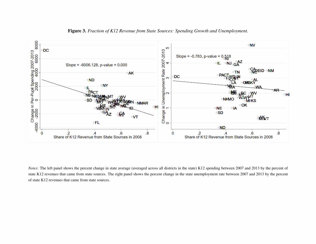
Figure 3. Fraction of K12 Revenue from State Sources: Spending Growth and Unemployment.

Notes: The left panel shows the percent change in state average (averaged across all districts in the state) K12 spending between 2007 and 2013 by the percent ofstate K12 revenues that came from state sources. The right panel shows the percent change in the state unemployment rate between 2007 and 2013 by the percentof state K12 revenues that came from state sources.

Figure 4. Difference in Spending and Outcomes Between States with High and Low Reliance on State Revenues Over Time

Notes: The dashed connected lines depicts the coefficients on the individual calendar year indicators interacted with an indicator for hight reliance on state revenuein 2008, lnΩs > 0.33. The solid lines represent the linear fit during the pre-recession period/cohorts (negative values of exposure) and post recession periods/cohorts(non-negative values of exposure). The pattern for log per-pupil spending is presented in top-left panel; the pattern for test scores is presented in top-right panel; thepattern for college-going is in the bottom-left; and the slope between the poverty rate and NAEP scores is shown in the bottom-right.

Figure 5. Forrest Plot of Existing Studies

Notes: The Forrest plot comes from Jackson and Mackevicius (2020), an ongoing meta-analysis of school spendingstudies being conducted by Kirabo Jackson and Claire Mackevicius. To facilitate comparison across studies we willconvert each study’s outcome into standardized units. Standardize the treatment: When the effect of spending isreported, we record that estimate of the change in spending directly. However, some studies report the impacts of aparticular spending policy on outcomes. To allow for comparison across studies, we define each policy based on thechange in per-pupil spending (CPI adjusted to 2018 dollars) that results from that policy. Many studies measure studentoutcomes some years after the policy change so that the duration of exposure needs to be standardized across studies.To standardize both spending and duration of exposure to said spending, for each study, we compute the average changein per-pupil spending for the four years preceding the observed outcome induced by the policy. Standardized Effect:After standardizing both the outcome and the treatment, for each study, we compute the change in the standardizedoutcome per $1000 policy-induced increase in school spending averaged over four years. We report this effect for thefull population in each study along with the 95% confidence interval. For some studies, the policy induced spendingchange is very small so that the confidence intervals are very wide.

Table 1: Summary Statistics

(1) (2) (3)N Mean SD

School SpendingPer-pupil spending (2015 dollars) 459 13,355 3,841Share of revenue from state sources in 2008 (IV) 51 0.493 0.137Share of revenue from federal sources 459 0.0954 0.0334Share of revenue from state sources 459 0.487 0.139Share of revenue from local sources 459 0.417 0.144

Per-Pupil Spending By Use (2015 dollars per pupil)Elementary/Secondary (Operations) 459 11,364 3,196

Instructional 459 6,872 2,064Services 459 4,011 1,230

Capital 458 1,280 806.3Construction 456 918.6 609.5

Non-Construction 459 331.7 175.0Other 459 481.3 106.3Salaries/Benefits

Instructional Salaries 459 4,548 1,189Non-Instructional Salaries 459 2,208 560.2

Benefits 459 2,140 875.5

Students Per StaffTeachers 446 15.42 2.526Aides 427 66.29 26.44Guidance Counselors 440 446.67 146.15Library Staff 447 653.2 829.99

Demographics & Economic IndicatorsK12 Enrollment 459 943.6 1,113Total Population (thousands) 459 5,868.8 6,613.7Child-Age Population (thousands) 459 1,025.5 1,186.9% Total Population in Poverty 459 13.51 3.282% Child-Age Population in Poverty 459 17.00 5.240Unemployment Rate (Contemporaneous) 459 5.910 2.006Annual Average Employment (thousands) 459 2,610.7 2,830.6Zillow Home Value Index 456 179,170 83,884

OutcomesAverage NAEP Score 459 0.125 0.211Slope 390 -3.552 1.171College-Going Rate 408 0.526 0.0926

4-year schools 408 0.359 0.08002-year school 408 0.152 0.0638

Notes: All dollar amounts are CPI-adjusted to 2015. All variables are col-lected for each state in 2002, 2003, 2005, 2007, 2009, 2011, 2013, 2015, and2017. 2017 data was not available for school spending so we use 2016 datainstead. College enrollment rates were not available for 2016 or 2017. TheZillow Housing Value Index was not available for North Dakota in 2002, 2003,or 2005. NAEP Scores are standardized to 2003 scores using restricted-useindividual-level data.

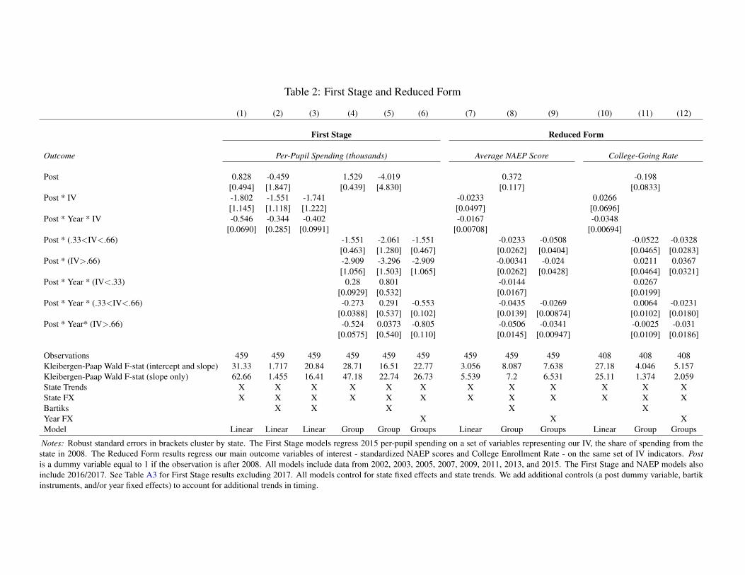
Table 2: First Stage and Reduced Form

(1) (2) (3) (4) (5) (6) (7) (8) (9) (10) (11) (12)

First Stage Reduced Form

Outcome Per-Pupil Spending (thousands) Average NAEP Score College-Going Rate

Post 0.828 -0.459 1.529 -4.019 0.372 -0.198[0.494] [1.847] [0.439] [4.830] [0.117] [0.0833]

Post * IV -1.802 -1.551 -1.741 -0.0233 0.0266[1.145] [1.118] [1.222] [0.0497] [0.0696]

Post * Year * IV -0.546 -0.344 -0.402 -0.0167 -0.0348[0.0690] [0.285] [0.0991] [0.00708] [0.00694]

Post * (.33<IV<.66) -1.551 -2.061 -1.551 -0.0233 -0.0508 -0.0522 -0.0328[0.463] [1.280] [0.467] [0.0262] [0.0404] [0.0465] [0.0283]

Post * (IV>.66) -2.909 -3.296 -2.909 -0.00341 -0.024 0.0211 0.0367[1.056] [1.503] [1.065] [0.0262] [0.0428] [0.0464] [0.0321]

Post * Year * (IV<.33) 0.28 0.801 -0.0144 0.0267[0.0929] [0.532] [0.0167] [0.0199]

Post * Year * (.33<IV<.66) -0.273 0.291 -0.553 -0.0435 -0.0269 0.0064 -0.0231[0.0388] [0.537] [0.102] [0.0139] [0.00874] [0.0102] [0.0180]

Post * Year* (IV>.66) -0.524 0.0373 -0.805 -0.0506 -0.0341 -0.0025 -0.031[0.0575] [0.540] [0.110] [0.0145] [0.00947] [0.0109] [0.0186]

Observations 459 459 459 459 459 459 459 459 459 408 408 408Kleibergen-Paap Wald F-stat (intercept and slope) 31.33 1.717 20.84 28.71 16.51 22.77 3.056 8.087 7.638 27.18 4.046 5.157Kleibergen-Paap Wald F-stat (slope only) 62.66 1.455 16.41 47.18 22.74 26.73 5.539 7.2 6.531 25.11 1.374 2.059State Trends X X X X X X X X X X X XState FX X X X X X X X X X X X XBartiks X X X X XYear FX X X XModel Linear Linear Linear Group Group Groups Linear Group Groups Linear Group Groups

Notes: Robust standard errors in brackets cluster by state. The First Stage models regress 2015 per-pupil spending on a set of variables representing our IV, the share of spending from thestate in 2008. The Reduced Form results regress our main outcome variables of interest - standardized NAEP scores and College Enrollment Rate - on the same set of IV indicators. Postis a dummy variable equal to 1 if the observation is after 2008. All models include data from 2002, 2003, 2005, 2007, 2009, 2011, 2013, and 2015. The First Stage and NAEP models alsoinclude 2016/2017. See Table A3 for First Stage results excluding 2017. All models control for state fixed effects and state trends. We add additional controls (a post dummy variable, bartikinstruments, and/or year fixed effects) to account for additional trends in timing.

Table 3: Revenue Sources

(1) (2) (3) (4) (5) (6) (7) (8) (9)

Per-Pupil Revenue by Source: Federal State Local

Post * IV 161 -969.7 -2,179[383.0] [1,424] [1,017]

Post * Year * IV -127.4 -173 -34.94[42.11] [81.72] [109.8]

Post * (.33<IV<.66) -41 55.64 -452.1 -409.7 -1,173 -756.7[158.6] [234.4] [200.0] [168.9] [1,378] [687.5]

Post * (IV>.66) 0.447 74.39 -2,439 -2,408 -1,319 -997.9[210.2] [256.9] [1,179] [1,200] [1,448] [920.7]

Post * Year * (IV<.33) 58.5 165.2 461[149.1] [132.4] [482.8]

Post * Year * (.33<IV<.66) 24.03 -41.88 19.41 -152.9 298.4 -197.8[119.5] [58.27] [131.9] [74.97] [419.9] [138.8]

Post * Year * (IV>.66) -5.634 -70.56 -457.4 -629.3 561.1 67.73[134.2] [68.81] [226.8] [196.8] [436.2] [187.1]

P(Post*Year*IV) 0.00393 0.0393 0.752P(Low=High) 0.306 0.31 0.00287 0.00241 0.527 0.719

Observations 459 459 459 459 459 459 459 459 459State Trends X X X X X X X X XState FX X X X X X X X X XPost*IV X X X X X X X X XPost X X XBartiks X X X X X XYear FX X X XModel Linear Group Group Linear Group Group Linear Group Group

Notes: Robust standard errors in brackets cluster by state. Data are collected from the F33 School District Finance survey. Allmodels include state-by-year observations for 2002, 2003, 2005, 2007, 2009, 2011, 2013, 2015, and 2016. All models control forstate fixed effects and state trends. Models 1, 2, 4, 5, 7, and 8 also include a state-level bartik instrument and 3 year-lagged bartikinstruments to control for additional economic timing trends. Models 3, 6, and 9 include year fixed effects in place of the bartikinstruments. Post is a dummy variable equal to 1 if the observation is after 2008. For models using the linear IV, P(Post*Year*IV)tests whether states with a higher reliance on state funds for K12 education in 2008 experienced a decline in the trend of eachrevenue source in the years after the Great Recession. In the Group IV models, P(Low=High) tests whether states with the highestreliance on state-funds experienced greater declines in each revenue source in the years post-Recession than the states with thelowest reliance on state funds.

Table 4: 2SLS Main Results

(1) (2) (3) (4) (5) (6) (7) (8) (9) (10) (11) (12)

Average NAEP Score College Enrollment Rate

Per-Pupil Spending (thousands) 0.0471 0.0698 0.0415 0.0502 0.0236 0.0441 0.0426 0.0574 0.0624 0.0384 0.026 0.0279[0.0103] [0.0925] [0.0190] [0.00966] [0.0106] [0.0131] [0.00693] [0.0331] [0.0159] [0.00584] [0.00856] [0.0106]

Pr(underid) 3.82E-07 0.182 0.00103 8.10E-07 0.0907 0.0505 9.84E-08 0.0373 0.00184 3.21E-07 0.09 0.0794Kleibergen-Paap Wald F-stat 62.66 1.455 16.41 47.18 22.74 26.73 78.85 8.281 21.45 52.29 7.886 10.17Pr(Endog) 5.63E-05 0.28 0.0597 1.03E-05 0.829 0.0708 2.91E-07 0.127 0.0027 2.45E-07 0.115 0.101

Predicted NAEP Score Predicted College Enrollment Rate

Per-Pupil Spending (thousands) 0.0187 -0.00844 0.00752 0.016 0.00037 0.000704 0.0139 -0.000392 0.00723 0.0112 0.00113 0.00144[0.00405] [0.0127] [0.00637] [0.00346] [0.00348] [0.00318] [0.00307] [0.00794] [0.00446] [0.00287] [0.00277] [0.00354]

Observations 459 459 459 459 459 459 408 408 408 408 408 408

State Trends X X X X X X X X X X X XState FX X X X X X X X X X X X XPost*IV X X X X X X X X X X X XPost X X X X X X X XBartiks X X X X X XYear FX X XModel Linear IV Linear IV Linear IV Group IV Group IV Group IV Linear IV Linear IV Linear IV Group IV Group IV Group IV

Notes: Robust standard errors in brackets cluster by state. Data are collected from the F33 School District Finance survey, IES NAEP results, and IPEDS. All models include state-by-year observations for 2002, 2003, 2005, 2007, 2009, 2011, 2013, and 2015. NAEP models also include 2016/2017. Post is a dummy variable equal to 1 if the observation is after 2008.We instrument for per-pupil spending here using Post*Year*IV in Linear models (columns 1-3 and 7-9) and Post*Year*[IV Group] in Group models (columns 4-6 and 10-12). The toppanel presents our main results regressing Average NAEP Scores and College Enrollment Rates on instrumented per-pupil spending. The bottom panel regresses the same outcomes aspredicted by economic and demographic variables (see table A2) on instrumented spending to demonstrate that instrumented spending is not endogenous to economic and demographiccharacteristics that are also correlated with academic outcomes.

Table 5: Spending Categories

(1) (2) (3) (4) (5) (6) (7) (8) (9) (10) (11) (12)

Overall Spending Category: Total Expenditures Capital Spending Elem/Sec Operating

Subset Spending Category: Capital Elem/Sec Operating Construction Instructional

Per-Pupil Spending (thousands) 267.3 571.1 482.9 778.6 353.4 475.4 306.7 478.5 441.7 618.8 446.9 472.3[130.9] [234.8] [223.4] [179.0] [189.1] [193.6] [137.6] [201.5] [190.6] [158.5] [51.40] [55.60]

Mean(Dependent Var.) 1280 1280 1280 11364 11364 11364 918.6 918.6 918.6 6872 6872 6872Average Share 0.0962 0.0962 0.0962 0.853 0.853 0.853 0.0691 0.0691 0.0691 0.515 0.515 0.515P(Average=Marginal) 0.197 0.0485 0.0896 0.679 0.011 0.0566 0.0905 0.0475 0.0562 0.515 0.193 0.449Observations 458 458 458 459 459 459 456 456 456 459 459 459

State Trends X X X X X X X X X X X XState FX X X X X X X X X X X X XPost*IV X X X X X X X X X X X XPost X X X XBartiks X X X X X X X XYear FX X X X XModel Linear IV Group IV Group IV Linear IV Group IV Group IV Linear IV Group IV Group IV Linear IV Group IV Group IV

Notes: Robust standard errors in brackets cluster by state. Data are collected from the F33 School District Finance survey. All models include state-by-year observations for 2002, 2003,2005, 2007, 2009, 2011, 2013, 2015, and 2016. Post is a dummy variable equal to 1 if the observation is after 2008. We instrument for per-pupil spending using Post*Year*IV in Linearmodels and Post*Year*[IV Group] in Group models. Coefficients on per-pupil spending can be interpreted as the amount of additional funds cut from each category for every one thousanddollars in exogenous educational spending cuts. More spending categories are reported in table A8.

Table 6: Staffing (2SLS)

(1) (2) (3) (4) (5) (6) (7) (8) (9) (10) (11) (12)

Teachers Aides Guidance Counselors Library Staff

Outcome: Log(Staff)

Per-Pupil Spending (thousands) 0.0763 0.0474 0.0407 0.092 0.0844 0.0587 0.0688 0.123 0.132 0.0669 0.033 0.102[0.0400] [0.0121] [0.00987] [0.0655] [0.0211] [0.0347] [0.0355] [0.0363] [0.0649] [0.0426] [0.0241] [0.0474]

Outcome: Log(Staff), controlling for Log(Enrollment)

Per-Pupil Spending (thousands) 0.0388 0.0152 0.0208 0.0551 0.0507 0.0307 0.0462 0.0893 0.116 0.0597 0.0137 0.1[0.0222] [0.0186] [0.0121] [0.0448] [0.0283] [0.0250] [0.0320] [0.0393] [0.0530] [0.0400] [0.0273] [0.0443]

Outcome: Students per Staff

Per-Pupil Spending (thousands) -0.5 -0.211 -0.292 -4.292 -2.443 -0.877 4.088 -66.41 -81.93 -22.16 -9.067 -66.23[0.302] [0.280] [0.206] [4.571] [1.469] [1.637] [21.55] [32.64] [39.65] [34.14] [21.76] [34.96]

Observations 446 446 446 427 427 427 440 440 440 447 447 447

State Trends X X X X X X X X X X X XState FX X X X X X X X X X X X XPost*IV X X X X X X X X X X X XPost X X X XBartiks X X X X X X X XYear FX X X X XModel Linear IV Group IV Group IV Linear IV Group IV Group IV Linear IV Group IV Group IV Linear IV Group IV Group IV

Notes: Robust standard errors in brackets cluster by state. Data are collected from the F33 School District Finance survey and the NCES Common Core of Data LEA Universe Survey.All models include state-by-year observations for 2002, 2003, 2005, 2007, 2009, 2011, 2013, 2015, and 2016/2017. Post is a dummy variable equal to 1 if the observation is after 2008.We instrument for per-pupil spending using Post*Year*IV in Linear models and Post*Year*[IV Group] in Group models. For each staff category (teachers, aides, guidance counselors, andlibrary staff) we estimate three panels. The first and second panels regresses the log of the staff count on instrumented per-pupil spending. The second panel also controls for the log of K12student enrollment. The third panel regresses the student:staff ratio on instrumented spending. For instance, the coefficient -.5 in column 1 panel 3 indicates that a $2,000 decline in per-pupilspending increases class size by one student per teacher on average. Not all states reported staff counts for each category in every year, but all states and years are represented in the sample.

Table 7: Race and Income (2SLS)

(1) (2) (3) (4) (5) (6) (7) (8) (9) (10) (11) (12)

Slope Average NAEP Score by Race

White Black Hispanic

Per-Pupil Spending (thousands) 0.412 0.428 0.386 0.099 0.0446 0.0296 0.0159 0.0353 0.0353 0.000587 0.0223 -0.00574[0.240] [0.158] [0.151] [0.0442] [0.0201] [0.00820] [0.0299] [0.0318] [0.0151] [0.0890] [0.0252] [0.0133]

Observations 390 390 390 452 452 452 392 392 392 402 402 402State Trends X X X X X X X X X X X XState FX X X X X X X X X X X X XPost*IV X X X X X X X X X X X XPost X X X XBartiks X X X X X X X XYear FX X X X XModel Linear IV Group IV Group IV Linear IV Group IV Group IV Linear IV Group IV Group IV Linear IV Group IV Group IV

Notes: Robust standard errors in brackets cluster by state. Data are collected from the F33 School District Finance survey and the NCES Public and restricted-use NAEP Data. All modelsinclude state-by-year observations for 2002, 2003, 2005, 2007, 2009, 2011, 2013, and 2015. Average NAEP Score by race results also include 2016/2017. Average NAEP Scores by raceare not available in every year for every state, though most states are represented in each sub-sample. Exceptions are Idaho, Montana, and Wyoming (no reported scores for black students)and Maine, Vermont, and West Virginia (no reported scores for hispanic students). The variable “Slope” is computed by regressing individual-level NAEP scores on the district povertyrate (in 2007) for each year in each state. Post is a dummy variable equal to 1 if the observation is after 2008. We instrument for per-pupil spending using Post*Year*IV in Linear modelsand Post*Year*[IV Group] in Group models. All models control for state fixed effects and state trends and include a subset of bartik instruments, year fixed effects, and/or a post dummyindicator to control for additional economic characteristics correlated with years.

Table 8: 2SLS: College Going by Institution Type

(1) (2) (3) (4) (5) (6) (7) (8) (9)

Overall 2-Year 4-Year

Per-Pupil Spending (thousands) 0.056 0.026 0.0279 0.035 0.0068 0.0102 0.0207 0.0171 0.0159[0.0107] [0.00856] [0.0106] [0.00656] [0.00493] [0.00482] [0.00781] [0.00997] [0.0119]

Average rate 0.526 0.152 0.359Effective % change 0.106 0.0495 0.0531 0.231 0.0448 0.0673 0.0578 0.0476 0.0443

Public (2 or 4 year) Private (2 or 4 year) More than 40% Part-Time (4 year)

Per-Pupil Spending (thousands) 0.0423 0.0191 0.0211 0.0134 0.00475 0.00499 0.00539 0.00326 0.00359[0.00834] [0.00379] [0.00355] [0.00333] [0.00567] [0.00653] [0.00199] [0.00181] [0.00199]

Average rate 0.388 0.122 0.011Effective % change 0.109 0.0493 0.0544 0.11 0.0388 0.0408 0.488 0.295 0.325

Less than 40% Part-Time (4 year) Selective/Most Selective (4 year) Minority Serving Institution (2 or 4 year)

Per-Pupil Spending (thousands) 0.0131 0.0134 0.0117 0.00881 0.00993 0.00846 0.0163 0.0169 0.0171[0.00663] [0.00806] [0.00972] [0.00555] [0.00616] [0.00733] [0.00696] [0.00672] [0.00787]

Average rate 0.333 0.294 0.0948Effective % change 0.0394 0.0403 0.0351 0.0299 0.0337 0.0287 0.172 0.178 0.18

Non-MSI (2 or 4 year) Hispanic-Serving Institutions (2 or 4 year) Non-HSI MSI (2 or 4 year)

Per-Pupil Spending (thousands) 0.0397 0.00915 0.0109 0.0045 0.0016 0.00206 0.0118 0.0153 0.015[0.0104] [0.00399] [0.00568] [0.00323] [0.00270] [0.00293] [0.00638] [0.00590] [0.00702]

Average rate 0.431 0.0205 0.0743Effective % change 0.092 0.0212 0.0252 0.219 0.0781 0.1 0.159 0.206 0.202

Observations 408 408 408 408 408 408 408 408 408State Trends X X X X X X X X XState FX X X X X X X X X XPost*IV X X X X X X X X XPost X X XBartiks X X X X X XYear FX X X XModel Linear IV Group IV Group IV Linear IV Group IV Group IV Linear IV Group IV Group IV

Notes: Robust standard errors in brackets cluster by state. Data are collected from the F33 School District Finance survey, IPEDS, IPUMS, and the CarnegieFoundation. All models include state-by-year observations for 2002, 2003, 2005, 2007, 2009, 2011, 2013, and 2015. Enrollment rates are calculated from the numberof first time enrollees at institutions meeting the stated criteria (e.g. public or 4-year) that graduated from high school in the past year, by which state the studentslived at the time of application (IPEDS), divided by the number of 17 year-olds 2 years prior to the enrollment year (IPUMS). We report the average enrollment rateat each type of institution over all states and years to scale the effects to be respective to each institution type’s representation in overall enrollment rates. Post is adummy variable equal to 1 if the observation is after 2008. We instrument for per-pupil spending using Post*Year*IV in Linear models and Post*Year*[IV Group] inGroup models. All models control for state fixed effects and state trends and include a subset of bartik instruments, year fixed effects, and/or a post dummy indicatorto control for additional economic characteristics correlated with years. Minority Serving Institutions and Hispanic-Serving Institutions are defined according to IESdefinitions (page V) using 2005 undergraduate enrollment data from IPEDS. Selective/Most Selective schools are those 4-year institutions that enroll fewer than 40%part-time students and admissions test scores are in the 40th to 100th percentile of selectivity. We use the Carnegie Classifications from 2005 for all institutions.Additional results by college type are reported in table A15.

Appendix

A Data on School Spending and ResourcesThe data on district level school finances is collected from the Census website.25 The underlying data comes from

the Common Core of Data (CCD) School District Finance Survey (F-33). It consists of data submitted annually to theNational Center for Education Statistics (NCES) by state education agencies (SEAs) in the 50 states and the Districtof Columbia. The purpose of the survey is to provide finance data for all local education agencies (LEAs) that providefree public elementary and secondary education in the United States. Both NCES and the Governments Division of theU.S. Census Bureau collect public school system finance data, and they collaborate in their efforts to gather these data.The F-33 data provides information on revenues, expenditures, and the number of students enrolled. Expendituresare reported in a number of categories including instructional spending, capital outlays, and administrative spending.Revenues are reported in several fine categories and aggregated to local, state, and federal sources. We CPI-adjust allspending variables to be in 2015 dollars and divide by district enrollment in the given year to obtain per-pupil spendingvariables.

The surveys are administered annually from 1992 onward. The last year for which data is available is the 2015-2016 academic year. We link together multiple years of data to create a balanced state-year panel (summarizing firstacross school districts). In constructing the data set, we found that the financial data contained some extremely largeand small values. These values could be valid, but it is more likely that some districts incorrectly reported enrollmentsor expenditures. We therefore censored the data by winsorizing extreme values. First, we calculated the (unweighted)99th and 1st percentile district in total per-pupil current expenditures for each state and year. We then capped valuesof districts with per-pupil expenditures at greater than 200 per-cent of the 99th percentile of per-pupil revenues or lessthan 50 percent of the 1st percentile.

For school spending categories (such as capital or instructional salaries), we replace values with missing wherethe CPI-adjusted per-student categorical spending value is more than twice the 99th percentile. We follow a similarstrategy for reported staffing categories, which come from the NCES Common Core of Data LEA Universe surveys(CCD), replacing staffing values with missing if the total staffing variable or the staffing per student (or students perstaff) is more than twice the 99th percentile. Note that not all states report staffing data in every year, and so ourstate-by-year analytic sample for staffing estimates is not balanced.

B Recession Intensity & Employment DataImportant to our identification strategy is controlling for the direct effect of broader recessionary economic condi-

tions. For this purpose, we construct an index of recession severity and exposure. We exploit the fact that the impact ofrecession varied on basis of local industrial compositions and create a shift-share instrument, along the lines of Bartik(1991), which captures changes in economic conditions attributable to the onset of the recession.

To do so, we follow the steps broadly outlined in Yagan (2017). We retrieve average annual county-level em-ployment data from the Quarterly Census of Employment and Wages (QCEW).26 Each state’s time-varying shift-share

25For instance, data for the school year 2015-2016 is available at https://www.census.gov/data/tables/2015/econ/school-finances/secondary-education-finance.html and data for the other years can be re-trieved by modifying the appropriate part of the url.

26The QCEW program publishes an annual count of employment and wages reported by employers covering 98 per-cent of U.S. jobs, available at the county, MSA, state and national levels by industry. Average annual data were down-loaded from the Bureau of Labor Statistics for each county and year from https://www.bls.gov/cew/datatoc.

shock is computed as the projected unemployment in each year, based on the interaction between the 2007 (pre-recession) employment composition by two-digit NAICS industry categories and the nationwide unemployment by thesame groupings in that year. Formally, in state s during year t the instrument equals:

Bartik Predictorst = ∑j

(E js2007

∑ j′ E j′s2007×National Unemployment jst

)(8)

where j denotes a two-digit industry, E js2007 denotes total employment in industry j in state s in 2007, andNational Unemployment jt is the nationwide unemployment rate in industry j in state s in year t.

From the same dataset (QCEW) above, we also compile the annual total employment number in each county as anadditional measure of economic status. As an additional economic indicator, we obtain state-level estimates of housingvalues from Zillow and use the January index for each year as an annual indicator of home prices.

C NAEP DataFor our main analyses, we use publicly available state-level NAEP test score data from the National Center for

Education Statistics. The NAEP is administered every other year to a population-weighted sample of schools andstudents. Schools are selected from 94 geographic areas, 22 of which are always the same major metropolitan areas.Students are selected randomly within the selected schools to complete the assessments. Note that our main results areinvariant to the use of sampling weights.

We use restricted-use individual-level for three purposes: 1) to compute average private school scores, 2) to com-pute the relationship between district poverty rates and NAEP scores, and 3) to compute the mean and standard devi-ation of all scores in 2003 for standardization. We infix the raw files to Stata, including all plausible score values perstudent, and restricting the sample to the NAEP reporting sample and public private school students (for 2 and 3) orprivate school students (for 1). The restriction to the reporting sample and public school students corresponds directlyto the sample used to calculate state averages as reported publicly by NCES.

Our dependent variable in all public-school NAEP estimations is the average of all publicly available scores perstate, year, grade, and subject, standardized to the base year of 2003 (determined from the restricted-use individual-level scores). We also use publicly available scores by race in the same way. We restrict our analyses to the years 2002and later, as NAEP sampling increased dramatically after 2001 and testing years became more consistent at this time.

D College Enrollment DataOur college-going data are obtained from the the Integrated Postsecondary Education Data System (IPEDS). These

data report surveys submitted at the aggregate-level from postsecondary institutions. These data do not have student-level information. Institutions report on the number of first-time college freshman from each state in each year whograduated high school in the past 12 months. By aggregating these data to the state of origin level, we obtain countsfor the number of first-time freshmen from each state in each year. We drop years where the survey was optional,and match each year of college enrollment to spending data from the year prior (when enrolling students would havegraduated high school). To compute college-going rates for these years, we obtain population counts by age in eachstate in each year from the American Community Surveys (ACS) from 2000 to 2016. Our college-going measure isthe number of first-time college enrollees divided by the number of 17-year-olds in the state two years prior to the yearof enrollment. We use this lagged cohort measure instead of 18-year olds in the year prior to minimize measurementerror from counting individuals who had already enrolled in college or moved away from home.

htm

Using information on postsecondary institutions from IPEDS and the Carnegie Foundation, we are able to computeenrollments by college type (2-year vs 4-year), selectivity level, and other characteristics about populations served. Weuse information on institution characteristics from Carnegie in 2005. Given that some institutional classifications arebased on the populations served, which may be endogenously affected by the recession and K12 spending cuts, weclassify institutions based on their 2005 categories for every year in our data. The Carnegie data provides informationfrom IPEDS on the level served (2 or 4 year) and control (public or private), as well as its own selectivity and part-time enrollment categories. Per their definitions, Inclusive 4-year institutions are those for whom test score data wasnot available or otherwise indicated that admissions were offered inclusively. Selective 4-year institutions were thosewith test scores that placed them between the 40th and 80th percentiles in selectivity, and More/Most Selective 4-yearinstitutions were those with thest scores that placed them between the 80th and 100th percentiles in selectivity.

The Carnegie data also includes IPEDS categories to note Historically Black Colleges and Universities (HBCU’s)and Tribal Colleges. However, we use 2005 IPEDS fall enrollment data by race to define categories for MinorityServing Institutions, Hispanic Serving Institutions, and Black Serving Institutions using IES definitions (page V ofthis document). We define these categories ourselves because exact definitions for 2005 were not available and thedata reported by Carnegie did not seem to match any known definitions precisely (for example, not all HBCU’s weredesignated as MSI’s).

Table A1: NAEP Availability

4th Grade 8th Grade 4th Grade 8th Grade TestedYear Math Math Reading Reading Students2015 X X X X 43043820142013 X X X X 57529820122011 X X X X 61978920102009 X X X X 57130820082007 X X X X 62022020062005 X X X X 58945820042003 X X X X 6422442002 X X 24022820012000 X X X 2224619991998 X X 1539119971996 X X 1080519951994 X 603019931992 X X X 16719

Notes: This table reports the availability of NAEP scores by year, grade,and subject using restricted-use individual NAEP data.

Table A2: Predicted Outcomes

(1) (2)Outcome Average

NAEP ScoreCollegeEnrollmentRate

Unemployment Rate (4yr) 0.0163 -0.00753[0.00451] [0.00405]

Unemployment Rate (1yr) 0.0064 -0.000171[0.00195] [0.00272]

% Total Population in Poverty 0.00572 0.013[0.00980] [0.00751]

% Child Population in Poverty -0.0166 -0.00601[0.00919] [0.00928]

Log (Child Population) -0.525 -0.512[0.222] [0.261]

Log (Total Population) 0.364 -0.0499[0.411] [0.376]

Log (Child Population in Poverty) 0.176 0.109[0.102] [0.133]

Annual Average Employment 5.08E-08 4.68E-08[1.82e-08] [2.63e-08]

Constant -0.461 6.7[5.301] [4.758]

Observations 459 408R-squared 0.963 0.839Within R-Squared 0.211 0.0853State FX X XState Trends X X

Notes: Robust standard errors in brackets cluster by state. Weregress outcomes on economic and demographic covariates, statefixed effects, and state trends and create linear predictions of theoutcomes based on the model. The samples here include state byyear observations for 2002, 2003, 2005, 2007, 2009, 2011, 2013,and 2015. Column 1 also includes data from 2017. Predicted out-comes are used as placebo outcome measures in our main resultsreported in table A17.

Table A3: First Stage, College-Going Sample (No 2017)

(1) (2) (3) (4) (5) (6)

Per-Pupil Spending (thousands)

Post 0.309 0.136 1.103 -5.62[0.603] [1.483] [0.263] [4.554]

Post * IV -0.56 -0.417 -0.373[1.297] [1.279] [1.081]

Post * Year * IV -0.677 -0.576 -0.558[0.0763] [0.200] [0.120]

Post * (.33<IV<.66) -0.992 -1.67 -0.992[0.297] [0.969] [0.300]

Post * (IV>.66) -2.312 -2.811 -2.312[1.009] [1.291] [1.018]

Post * Year * (IV<.33) 0.493 1.143[0.316] [0.614]

Post * Year * (.33<IV<.66) -0.339 0.395 -0.833[0.0427] [0.481] [0.322]

Post * Year* (IV>.66) -0.61 0.107 -1.103[0.0638] [0.481] [0.326]

Observations 408 408 408 408 408 408Kleibergen-Paap Wald F-stat (all) 40.58 4.163 17.52 32.26 6.914 9.891Kleibergen-Paap Wald F-stat (slope only) 78.85 8.281 21.45 52.29 7.886 10.17State Trends X X X X X XState FX X X X X X XBartiks X X X XYear FX XInstrument Linear Linear Linear Groups Groups Groups

Notes: Robust standard errors in brackets cluster by state. This table replicates the first stage panel oftable 2 dropping 2017 in order to correspond to the college-going sample. These results can be interpretedas the first stage for the 2SLS models when we examine the outcome College Enrollment Rate.

Table A4: OLS Models

(1) (2) (3) (4) (5) (6)

Average NAEP Score College Enrollment Rate

Per-Pupil Spending (thousands) 0.0109 0.00795 0.00465 0.0112 0.0124 0.00868[0.00364] [0.00359] [0.00314] [0.00268] [0.00294] [0.00439]

Observations 459 459 459 408 408 408State Trends X X X X X XState FX X X X X X XBartiks X XYear FX X X

Notes: Robust standard errors in brackets cluster by state. State-by-year observations include all states in years2002, 2003, 2005, 2007, 2009, 2011, 2013, and 2015. Models predicting NAEP scores also include 2016/2017.For each column, we regress the outcome (Average NAEP Score or College Enrollment Rate) on per-pupilspending, state fixed effects, and state trends. Models 2 and 5 also control for a series of bartik instruments,and models 3 and 6 include year fixed effects.

Table A5: 2SLS Models with Year Fixed Effects and Linear IV

(1) (2)

AverageNAEP Score

CollegeEnrollmentRate

Per-Pupil Spending (thousands) 0.00146 0.0374[0.0357] [0.0102]

Observations 459 408Pr(underid) 0.0759 0.129Kleibergen-Paap Wald F-stat 8.495 5.332Pr(Endog) 0.92 0.135State Trends X XState FX X XPost*IV X XYear FX X XModel Linear IV Linear IV

Notes: Robust standard errors in brackets cluster by state. State-by-year observations include all states in years 2002, 2003, 2005,2007, 2009, 2011, 2013, and 2015. Models predicting NAEP scoresalso include 2016/2017. Each column reports 2SLS results for theeffect of instrumented per-pupil spending on outcomes, using ourlinear instrument for spending (share of state spending in 2008).The excluded instrument in these models is Post*Year*IV. Modelshere include state fixed effects, state trends, and year fixed effects.The Kleibergen-Paap Wald F-stat reports the first stage F-statisticfor each model.

Table A6: 2SLS Main Effects, Log Specification

(1) (2) (3) (4) (5) (6) (7) (8) (9) (10) (11) (12)

Average NAEP Score College Enrollment Rate

Log (Per-Pupil Spending) 0.567 0.691 0.436 0.621 0.505 0.618 0.513 0.727 0.758 0.494 0.437 0.444[0.128] [0.697] [0.191] [0.126] [0.187] [0.215] [0.0804] [0.422] [0.181] [0.0757] [0.204] [0.221]

Pr(underid) 2.99E-07 0.0583 0.000329 4.45E-07 0.133 0.0674 6.49E-08 0.0329 0.000598 1.64E-07 0.137 0.0843Kleibergen-Paap Wald F-stat 67.61 3.749 28.3 31.79 17.46 28.56 90.41 8.548 30.82 35.93 11.73 10.58Pr(Endog) 5.33E-05 0.276 0.0755 5.68E-06 0.393 0.0634 8.31E-07 0.117 0.00213 1.94E-07 0.0705 0.0767

Predicted NAEP Score Predicted College Enrollment Rate

Log (Per-Pupil Spending) 0.225 -0.0836 0.0791 0.205 0.00095 0.00682 0.167 -0.00497 0.0879 0.152 0.0166 0.0217[0.0480] [0.107] [0.0665] [0.0431] [0.0496] [0.0463] [0.0361] [0.101] [0.0529] [0.0350] [0.0475] [0.0568]

Observations 459 459 459 459 459 459 408 408 408 408 408 408

State Trends X X X X X X X X X X X XState FX X X X X X X X X X X X XPost*IV X X X X X X X X X X X XPost X X X X X X X XBartiks X X X X X XYear FX X XModel Linear IV Linear IV Linear IV Group IV Group IV Group IV Linear IV Linear IV Linear IV Group IV Group IV Group IV

Notes: This table replicates table A17 using the Log of Per-Pupil Spending (2015 dollars) instead of Per-Pupil Spending (2015 thousands of dollars). Robust standard errors inbrackets cluster by state. Data are collected from the F33 School District Finance survey, IES NAEP results, and IPEDS. All models include state-by-year observations for 2002,2003, 2005, 2007, 2009, 2011, 2013, and 2015. NAEP models also include 2016/2017. We instrument for the log of per-pupil spending here using Post*Year*IV in Linear models(columns 1-3 and 7-9) and Post*Year*[IV Group] in Group models (columns 4-6 and 10-12). The top panel presents our main results regressing Average NAEP Scores and CollegeEnrollment Rates on instrumented log spending. The bottom panel regresses the same outcomes as predicted by economic and demographic variables (see table A2) on instrumentedlog spending to demonstrate that instrumented spending is not endogenous to economic and demographic characteristics that are also correlated with academic outcomes.

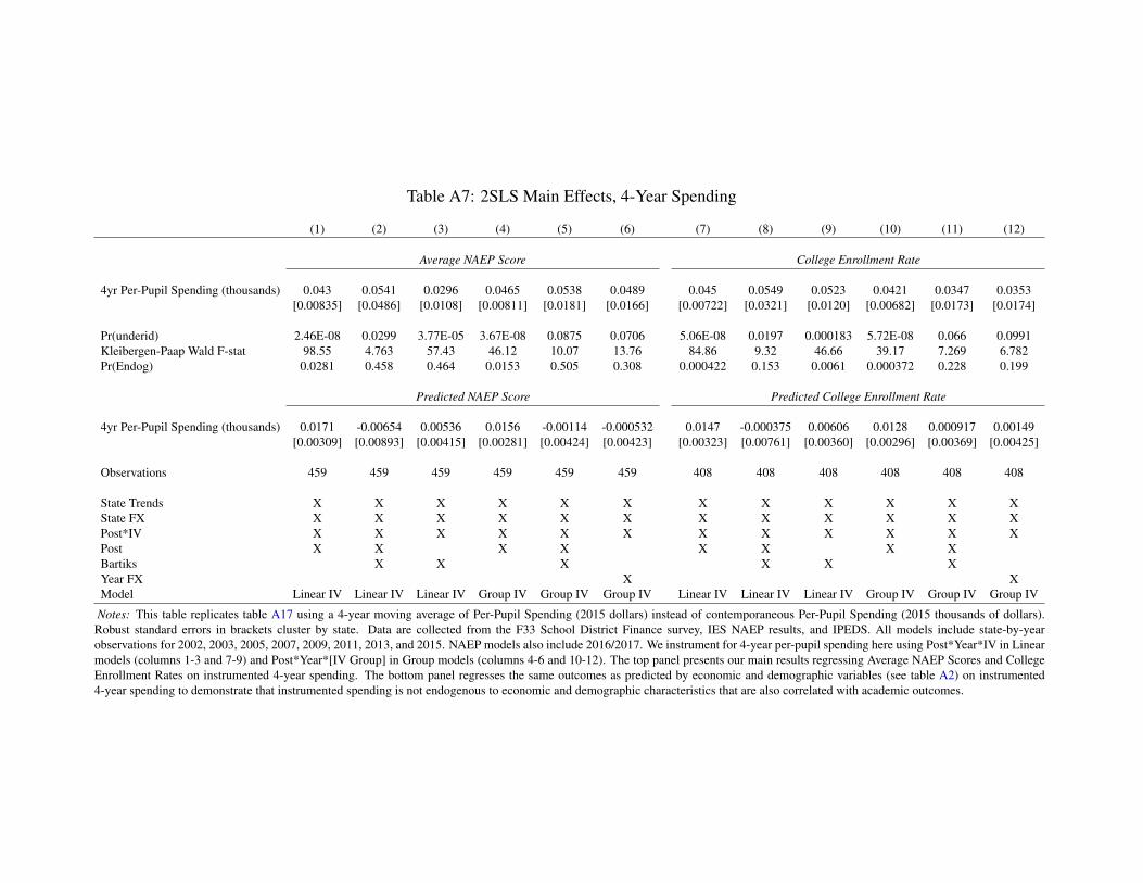
Table A7: 2SLS Main Effects, 4-Year Spending

(1) (2) (3) (4) (5) (6) (7) (8) (9) (10) (11) (12)

Average NAEP Score College Enrollment Rate

4yr Per-Pupil Spending (thousands) 0.043 0.0541 0.0296 0.0465 0.0538 0.0489 0.045 0.0549 0.0523 0.0421 0.0347 0.0353[0.00835] [0.0486] [0.0108] [0.00811] [0.0181] [0.0166] [0.00722] [0.0321] [0.0120] [0.00682] [0.0173] [0.0174]

Pr(underid) 2.46E-08 0.0299 3.77E-05 3.67E-08 0.0875 0.0706 5.06E-08 0.0197 0.000183 5.72E-08 0.066 0.0991Kleibergen-Paap Wald F-stat 98.55 4.763 57.43 46.12 10.07 13.76 84.86 9.32 46.66 39.17 7.269 6.782Pr(Endog) 0.0281 0.458 0.464 0.0153 0.505 0.308 0.000422 0.153 0.0061 0.000372 0.228 0.199

Predicted NAEP Score Predicted College Enrollment Rate

4yr Per-Pupil Spending (thousands) 0.0171 -0.00654 0.00536 0.0156 -0.00114 -0.000532 0.0147 -0.000375 0.00606 0.0128 0.000917 0.00149[0.00309] [0.00893] [0.00415] [0.00281] [0.00424] [0.00423] [0.00323] [0.00761] [0.00360] [0.00296] [0.00369] [0.00425]

Observations 459 459 459 459 459 459 408 408 408 408 408 408

State Trends X X X X X X X X X X X XState FX X X X X X X X X X X X XPost*IV X X X X X X X X X X X XPost X X X X X X X XBartiks X X X X X XYear FX X XModel Linear IV Linear IV Linear IV Group IV Group IV Group IV Linear IV Linear IV Linear IV Group IV Group IV Group IV

Notes: This table replicates table A17 using a 4-year moving average of Per-Pupil Spending (2015 dollars) instead of contemporaneous Per-Pupil Spending (2015 thousands of dollars).Robust standard errors in brackets cluster by state. Data are collected from the F33 School District Finance survey, IES NAEP results, and IPEDS. All models include state-by-yearobservations for 2002, 2003, 2005, 2007, 2009, 2011, 2013, and 2015. NAEP models also include 2016/2017. We instrument for 4-year per-pupil spending here using Post*Year*IV in Linearmodels (columns 1-3 and 7-9) and Post*Year*[IV Group] in Group models (columns 4-6 and 10-12). The top panel presents our main results regressing Average NAEP Scores and CollegeEnrollment Rates on instrumented 4-year spending. The bottom panel regresses the same outcomes as predicted by economic and demographic variables (see table A2) on instrumented4-year spending to demonstrate that instrumented spending is not endogenous to economic and demographic characteristics that are also correlated with academic outcomes.

Table A8: 2SLS: Additional Spending Categories

(1) (2) (3) (4) (5) (6) (7) (8) (9) (10) (11) (12) (13) (14) (15)

Overall Spending Category: Elem/Sec Operating Salaries & Benefits

Subset Spending Category: Support Services Instructional Salaries Non-Instructional Salaries Instructional Benefits Non-Instructional Benefits

Per-Pupil Spending (thousands) 166.6 -93.45 -3.721 228.7 243.4 282.9 113.5 -32.08 -0.191 312.5 196 228.2 119.4 -33.98 -43.37[110.9] [161.2] [162.2] [78.59] [55.23] [85.64] [49.88] [61.48] [58.74] [101.2] [65.84] [96.78] [104.4] [82.68] [93.84]

Mean(Dependent Var.) 4011 4011 4011 4548 4548 4548 2208 2208 2208 1408 1408 1408 732.3 732.3 732.3Average Share 0.3 0.3 0.3 0.344 0.344 0.344 0.168 0.168 0.168 0.105 0.105 0.105 0.055 0.055 0.055P(Average=Marginal) 0.233 0.0181 0.0666 0.149 0.0745 0.479 0.281 0.00205 0.00615 0.0457 0.173 0.209 0.54 0.287 0.3Observations 459 459 459 459 459 459 459 459 459 459 459 459 459 459 459

State Trends X X X X X X X X X X X X X X XState FX X X X X X X X X X X X X X X XPost*IV X X X X X X X X X X X X X X XPost X X X X XBartiks X X X X X X X X X XYear FX X X X X XModel Linear IV Group IV Group IV Linear IV Group IV Group IV Linear IV Group IV Group IV Linear IV Group IV Group IV Linear IV Group IV Group IV

Notes: Robust standard errors in brackets cluster by state. Data are collected from the F33 School District Finance survey. All models include state-by-year observations for 2002, 2003, 2005, 2007, 2009, 2011, 2013, 2015, and2016. We instrument for per-pupil spending using Post*Year*IV in Linear models and Post*Year*[IV Group] in Group models. Coefficients on per-pupil spending can be interpreted as the amount of additional funds cut fromeach category for every one thousand dollars in exogenous educational spending cuts. More spending categories are reported in table 5.

Table A9: Private School NAEP Scores (2SLS)

(1) (2) (3)

Private School NAEP Score

Per-Pupil Spending (thousands) -0.134 -0.0111 0.0429[0.116] [0.0394] [0.0343]

Observations 388 388 388

State Trends X X XState FX X X XPost*IV X X XPost XBartiks X XYear FX XModel Linear IV Group IV Group IV

Notes: Robust standard errors in brackets cluster by state. Spendingdata come from the F33 School District Finance survey. We calcu-late private school NAEP scores using the restricted-use NAEP data.We calculate NAEP scores for private school students, standardizingto 2003 private school NAEP scores. We take the mean for each stateand year, weighting by the ORIGWT sampling weight. We are notable to calculate a mean private school NAEP score for every state andyear, but all states and years are represented in the sample. All modelsinclude state-by-year observations for 2002, 2003, 2005, 2007, 2009,2011, 2013, and 2015. We instrument for per-pupil spending here us-ing Post*Year*IV in the Linear model (column 1) and Post*Year*[IVGroup] in Group models (columns 2 and 3).

Table A10: Exogeneity Test of Instrument (2SLS)

(1) (2) (3) (4) (5) (6)

Unemployment Rate (1yr) Unemployment Rate (4yr)

Per-Pupil Spending (thousands) 0.179 -0.0111 0.0607 -0.0729 -0.0267 -0.0476[0.496] [0.166] [0.187] [0.267] [0.146] [0.155]

Child Poverty Population Log(Child Poverty Population)

Per-Pupil Spending (thousands) -9,471 -1,789 -4,645 0.0112 -0.00872 -0.0162[7,689] [4,197] [5,139] [0.0311] [0.0291] [0.0373]

Annual Average Employment Employment Ratio*

Per-Pupil Spending (thousands) 50,695 12,664 15,640 0.0244 -0.00441 0.00429[56,942] [15,134] [13,721] [0.00976] [0.00781] [0.00883]

K12 Enrollment Log(K12 Enrollment)

Per-Pupil Spending (thousands) 15,732 -54.94 -3,537 0.042 0.0328 0.0221[8,236] [8,158] [9,379] [0.0353] [0.0178] [0.0215]

White Population Black Population

Per-Pupil Spending (thousands) 7,988 595.3 3,557 316,019 -53,132 5,954[6,144] [5,211] [5,668] [214,896] [87,864] [93,591]

Observations 459 459 459 459 459 459

State Trends X X X X X XState FX X X X X X XPost*IV X X X X X XPost X XBartiks X X X XYear FX X XModel Linear IV Group IV Group IV Linear IV Group IV Group IV

Notes: Robust standard errors in brackets cluster by state. Spending data are collected from the F33 SchoolDistrict Finance survey. Other data sources include BLS, SAIPE, NCES CCD, Zillow, and ACS. All mod-els include state-by-year observations for 2002, 2003, 2005, 2007, 2009, 2011, 2013, 2015, and 2016/2017.We instrument for per-pupil spending here using Post*Year*IV in Linear models (columns 1 and 4) andPost*Year*[IV Group] in Group models (columns 2-3 and 5-6). We regress each economic of demographicvariable on instrumented per-pupil spending. All models include state fixed effects and state trends. Columns1, 2, 4, and 5 also control for a series of lagged bartik instruments. Columns 3 and 6 instead control for yearfixed effects.*Employment ratio = Log(Annual Average Employment) - Log(Total Population)

Table A11: Saturated Models (2SLS)

(1) (2) (3) (4) (5) (6) (7) (8) (9) (10) (11) (12)

Model 1 Model 2 Model 3

Average NAEP Score

Per-Pupil Spending (thousands) 0.0415 0.0463 0.0691 0.106 0.0236 0.0331 0.00688 0.0036 0.0441 0.0568 0.0648 0.0607[0.0190] [0.0200] [0.0356] [0.0649] [0.0106] [0.0156] [0.0160] [0.0157] [0.0131] [0.0310] [0.0296] [0.0249]

Observations 459 459 459 456 459 459 459 456 459 459 459 456

College Enrollment Rate

Per-Pupil Spending (thousands) 0.0624 0.0659 0.0867 0.0617 0.026 0.0273 0.0268 0.0273 0.0279 0.0296 0.0297 0.0279[0.0159] [0.0172] [0.0310] [0.0329] [0.00856] [0.0139] [0.0125] [0.0127] [0.0106] [0.0173] [0.0160] [0.0154]

Observations 408 408 408 405 408 408 408 405 408 408 408 405

State Trends & State FX X X X X X X X X X X X XPost*IV X X X X X X X X X X X XPost X X X XBartiks X X X X X X X XYear FX X X X XPopulation Controls X X X X X X X X XEconomic Controls X X X X X XHousing Values X X XModel Linear IV Linear IV Linear IV Linear IV Group IV Group IV Group IV Group IV Group IV Group IV Group IV Group IV

Notes: Robust standard errors in brackets cluster by state. All models include state-by-year observations for 2002, 2003, 2005, 2007, 2009, 2011, 2013, and 2015. NAEP models alsoinclude 2016/2017. We instrument for per-pupil spending here using Post*Year*IV in Linear models (columns 1-3 and 7-9) and Post*Year*[IV Group] in Group models (columns 4-6and 10-12). The top and bottom panels present results regressing Average NAEP Scores or College Enrollment rates on instrumented per-pupil spending. Each set of models builds ona preferred specification from our main results in table A17. Column (1) directly replicates the results presented in columns (3) and (9) from table A17. Column (2) adds populationcontrols (total population and child population), column (3) adds economic controls (1 and 4 year unemployment rates, child poverty rate, total poverty rate, and log(employment)), andcolumn (4) adds a control for the housing value index (not available for North Dakota in 2002, 2003, or 2005). COlumn (5) replicates the model from columns (5) and (11) from tableA17. Column (9) here replicates models from columns (6) and (12) from A17. We add additional population and economic controls to each of these preferred specficications followingthe same progression as in columns (1) through (4).

Table A12: 2SLS Main Results: Alternative IV for California

(1) (2) (3) (4) (5) (6) (7) (8) (9) (10) (11) (12)

Average NAEP Score College Enrollment Rate

Per-Pupil Spending (thousands) 0.047 0.0706 0.0413 0.0503 0.0221 0.0441 0.0427 0.0598 0.0638 0.0387 0.0265 0.0285[0.0103] [0.103] [0.0194] [0.00987] [0.0116] [0.0139] [0.00689] [0.0343] [0.0160] [0.00587] [0.00849] [0.0106]

Observations 459 459 459 459 459 459 408 408 408 408 408 408Pr(underid) 3.54E-07 0.234 0.00135 8.27E-07 0.126 0.0713 9.32E-08 0.0396 0.00166 3.30E-07 0.0854 0.0779Kleibergen-Paap Wald F-stat 60.63 1.133 13.35 29.43 16.69 19.17 78.72 7.098 18.63 42.09 6.726 7.4Pr(Endog) 5.47E-05 0.319 0.0689 1.07E-05 0.558 0.129 2.73E-07 0.113 0.0017 2.14E-07 0.0836 0.0706

State Trends X X X X X X X X X X X XState FX X X X X X X X X X X X XPost*IV X X X X X X X X X X X XPost X X X X X X X XBartiks X X X X X XYear FX X XModel Linear IV Linear IV Linear IV Group IV Group IV Group IV Linear IV Linear IV Linear IV Group IV Group IV Group IV

Notes: This table replicates the top panel of table A17 using an alternative specification of our instrument for California. The majority of school district property tax revenue inCalifornia is collected and redistributed by the State. In our main models, we classify this revenue as ”local.” In results presented here, we re-classify property tax revenue reported byindependent school districts as ”state” revenue instead. This causes our instrument for California (share of 2008 education revenues from state sources) to increase from .58 to .78.Robust standard errors in brackets cluster by state. Data are collected from the F33 School District Finance survey, IES NAEP results, and IPEDS. All models include state-by-yearobservations for 2002, 2003, 2005, 2007, 2009, 2011, 2013, and 2015. NAEP models also include 2016/2017. We instrument for per-pupil spending here using Post*Year*IV in Linearmodels (columns 1-3 and 7-9) and Post*Year*[IV Group] in Group models (columns 4-6 and 10-12). We regress Average NAEP Scores and College Enrollment Rates on instrumentedspending.

Table A13: 2SLS Main Results: Dropping States

(1) (2) (3) (4) (5) (6) (7) (8) (9) (10) (11) (12)

Average NAEP Score College Enrollment Rate

Dropping DC

Per-Pupil Spending (thousands) 0.0471 0.0181 0.0374 0.05 0.055 0.0368 0.0426 0.0339 0.0688 0.0399 0.0164 0.015[0.0103] [0.0319] [0.0178] [0.00991] [0.0202] [0.0166] [0.00693] [0.0264] [0.0199] [0.00619] [0.0102] [0.00903]

Observations 450 450 450 450 450 450 400 400 400 400 400 400Pr(underid) 3.82E-07 0.04 0.000827 1.25E-06 0.0874 0.0758 9.84E-08 0.0646 0.00148 4.20E-07 0.132 0.0787Kleibergen-Paap Wald F-stat 62.63 6.352 23.08 45.59 14.55 20.84 78.81 5.407 23.36 51.92 10.94 15.62Pr(Endog) 5.66E-05 0.691 0.101 1.89E-05 0.00303 0.111 2.96E-07 0.21 0.00583 3.39E-07 0.311 0.316

Dropping CA

Per-Pupil Spending (thousands) 0.0474 0.0696 0.0411 0.0505 0.0232 0.0442 0.0422 0.0551 0.0613 0.0381 0.0263 0.0279[0.0105] [0.0902] [0.0189] [0.00979] [0.0106] [0.0131] [0.00705] [0.0325] [0.0159] [0.00590] [0.00854] [0.0106]

Observations 450 450 450 450 450 450 400 400 400 400 400 400Pr(underid) 5.18E-07 0.168 0.000809 1.08E-06 0.0922 0.0509 1.55E-07 0.0356 0.00169 4.94E-07 0.0892 0.0796Kleibergen-Paap Wald F-stat 61.5 1.543 17.08 46.74 22.76 26.69 75.21 8.517 21.67 51.25 7.886 10.12Pr(Endog) 6.80E-05 0.272 0.0591 1.30E-05 0.828 0.0713 4.96E-07 0.142 0.00314 3.95E-07 0.107 0.0992

Dropping HI

Per-Pupil Spending (thousands) 0.0489 0.103 0.0413 0.0522 0.0189 0.0479 0.0423 0.0517 0.0572 0.0379 0.0243 0.0268[0.0110] [0.176] [0.0239] [0.0103] [0.0116] [0.0138] [0.00742] [0.0448] [0.0182] [0.00622] [0.00908] [0.0116]

Observations 450 450 450 450 450 450 400 400 400 400 400 400Pr(underid) 4.53E-07 0.353 0.00156 1.31E-06 0.136 0.0792 8.80E-08 0.0576 0.00292 5.06E-07 0.111 0.12Kleibergen-Paap Wald F-stat 55.24 0.628 10.27 35.78 20.13 22.22 70.11 4.453 14.88 52.14 11.05 8.57Pr(Endog) 8.90E-05 0.3 0.106 1.47E-05 0.453 0.0492 4.26E-07 0.251 0.00397 4.03E-07 0.229 0.224

State Trends X X X X X X X X X X X XState FX X X X X X X X X X X X XPost*IV X X X X X X X X X X X XPost X X X X X X X XBartiks X X X X X XYear FX X XModel Linear IV Linear IV Linear IV Group IV Group IV Group IV Linear IV Linear IV Linear IV Group IV Group IV Group IV

Notes: This table replicates the top panel of table A17 dropping individual states from the analysis. Robust standard errors in brackets cluster by state. Data are collected from the F33School District Finance survey, IES NAEP results, and IPEDS. All models include state-by-year observations for 2002, 2003, 2005, 2007, 2009, 2011, 2013, and 2015. NAEP modelsalso include 2016/2017. We instrument for per-pupil spending here using Post*Year*IV in Linear models (columns 1-3 and 7-9) and Post*Year*[IV Group] in Group models (columns4-6 and 10-12). We regress Average NAEP Scores and College Enrollment Rates on instrumented spending, dropping either DC, California, or Hawaii from the sample to demonstratethe robustness of the main findings.

Table A14: Main Results (Weighted)

1 2 3 4 5 6 7 8 9 10 11 12

Average NAEP Score College Going Rate

Weight = K12 EnrollmentPer-Pupil Spending (thousands) 0.0603 -0.00329 0.0537 0.0565 0.0469 0.0255 0.0412 0.0218 0.054 0.0349 0.00332 0.00537

[0.0163] [0.0481] [0.0187] [0.0153] [0.0199] [0.00884] [0.00746] [0.0436] [0.0284] [0.00680] [0.00768] [0.00511]

Pr(underid) 7.26E-05 0.314 0.0278 0.000368 0.129 0.191 0.000105 0.228 0.00252 0.000315 0.183 0.183Kleibergen-Paap Wald F-stat 27.27 0.99 3.349 47.46 48.16 68.54 56.97 1.529 6.459 60.48 48.01 73.3Pr(Endog) 0.00325 0.714 0.0386 0.0285 0.00414 0.15 0.000143 0.463 0.00601 2.40E-05 0.193 0.12

Weight = Total PopulationPer-Pupil Spending (thousands) 0.06 0.00469 0.0566 0.0563 0.0479 0.0259 0.0405 0.0195 0.0504 0.0344 0.00356 0.00667

[0.0151] [0.0469] [0.0189] [0.0142] [0.0206] [0.00887] [0.00757] [0.0416] [0.0262] [0.00688] [0.00747] [0.00648]

Pr(underid) 9.30E-05 0.349 0.028 0.000503 0.141 0.183 9.13E-05 0.231 0.0021 0.000304 0.188 0.171Kleibergen-Paap Wald F-stat 25.27 0.852 3.49 48.3 49.84 70.79 51.03 1.524 7.184 56.91 44.37 67.13Pr(Endog) 0.00144 0.867 0.0278 0.0125 0.00386 0.138 0.000116 0.497 0.00639 2.33E-05 0.164 0.0845

Weight = Child-Aged PopulationPer-Pupil Spending (thousands) 0.0598 -0.00168 0.0526 0.0561 0.0467 0.0255 0.0411 0.0205 0.0529 0.0348 0.00324 0.00575

[0.0158] [0.0478] [0.0181] [0.0149] [0.0199] [0.00872] [0.00739] [0.0422] [0.0273] [0.00673] [0.00753] [0.00566]

Pr(underid) 6.90E-05 0.322 0.0261 0.000339 0.138 0.187 9.04E-05 0.223 0.00199 0.000265 0.188 0.177Kleibergen-Paap Wald F-stat 27.55 0.962 3.466 49.16 50.37 71.6 57.02 1.582 6.879 60.27 47.47 72.15Pr(Endog) 0.00253 0.748 0.0401 0.0231 0.00409 0.153 0.000124 0.478 0.00585 2.31E-05 0.184 0.105

Observations 459 459 459 459 459 459 408 408 408 408 408 408State Trends X X X X X X X X X X X XState FX X X X X X X X X X X X XPost*IV X X X X X X X X X X X XPost X X X X X X X XBartiks X X X X X XYear FX X XModel Linear IV Linear IV Linear IV Group IV Group IV Group IV Linear IV Linear IV Linear IV Group IV Group IV Group IV

Notes: This table replicates the top panel of table A17, weighting the regressions by population measures. Robust standard errors in brackets cluster by state. Data are collected fromthe F33 School District Finance survey, IES NAEP results, and IPEDS. All models include state-by-year observations for 2002, 2003, 2005, 2007, 2009, 2011, 2013, and 2015. NAEPmodels also include 2016/2017. We instrument for per-pupil spending here using Post*Year*IV in Linear models (columns 1-3 and 7-9) and Post*Year*[IV Group] in Group models(columns 4-6 and 10-12). We regress Average NAEP Scores and College Enrollment Rates on instrumented spending, weighting by either K12 enrollment, total population, or childpopulation in the state-year.

Table A15: 2SLS: College Going by Institution Type, Continued

(1) (2) (3) (4) (5) (6)

Black-Serving Institution Inclusive (4-year)

Per-Pupil Spending (thousands) 0.00617 0.00845 0.00792 0.00431 0.00349 0.00321[0.00209] [0.00431] [0.00497] [0.00182] [0.00204] [0.00247]

Average rate 0.047 0.0385Effective % change 0.131 0.18 0.168 0.112 0.0906 0.0834

Selective (4-year) Most Selective (4-year)

Per-Pupil Spending (thousands) 0.0109 0.00428 0.00435 -0.00212 0.00564 0.00411[0.00452] [0.00413] [0.00472] [0.00232] [0.00229] [0.00281]

Average rate 0.184 0.11Effective % change 0.0594 0.0233 0.0236 -0.0192 0.0512 0.0373

Observations 408 408 408 408 408 408State Trends X X X X X XState FX X X X X X XPost*IV X X X X X XPost X XBartiks X X X XYear FX X XModel Linear IV Group IV Group IV Linear IV Group IV Group IV

Notes: This table is a continuation of table 8. Robust standard errors in brackets cluster by state. Data are col-lected from the F33 School District Finance survey, IPEDS, IPUMS, and the Carnegie Foundation. All modelsinclude state-by-year observations for 2002, 2003, 2005, 2007, 2009, 2011, 2013, and 2015. Enrollment ratesare calculated from the number of first time enrollees at institutions meeting the stated criteria (e.g. inclusive)that graduated from high school in the past year, by which state the students lived at the time of application(IPEDS), divided by the number of 17 year-olds 2 years prior to the enrollment year (IPUMS). We report theaverage enrollment rate at each type of institution over all states and years to scale the effects to be respectiveto each institution type’s representation in overall enrollment rates. We instrument for per-pupil spending usingPost*Year*IV in Linear models and Post*Year*[IV Group] in Group models. All models control for state fixedeffects and state trends and include a subset of bartik instruments, year fixed effects, and/or a post indicatorto control for additional economic characteristics correlated with years. Black-Serving Institutions are definedaccording to IES definitions (page V) using 2005 undergraduate enrollment data from IPEDS. BSI’s includeHistorically Black Colleges and Universities or institutions where undergraduate enrollment is at least 25%black, and no other minority group makes up more than 25% of the undergraduate student body. Inclusive,Selective, and Most Selective schools are defined by Carnegie Classifications from 2005 for all institutions. In-clusive institutions are those for whom test scores are not available or suggests that admission is offered broadly.Selective institutions are those whose incoming test scores classify the institutions between the 40th and 80thpercentile of selectivity. Most Selective institutions fall between the 80th and 100th percentile in selectivity.

Table A16: NAEP by Grade and Subject (2SLS)

(1) (2) (3) (4) (5) (6)

Average NAEP Score

Math Reading

Per-Pupil Spending (thousands) 0.201 0.0017 0.063 -0.0258 0.0067 0.0169[0.0452] [0.0228] [0.0280] [0.0181] [0.00537] [0.00421]

Observations 408 408 408 454 454 454

4th Grade 8th Grade

Per-Pupil Spending (thousands) 0.0818 0.025 0.0511 0.0194 0.0209 0.0368[0.0224] [0.0152] [0.0187] [0.0175] [0.0110] [0.0108]

Observations 454 454 454 453 453 453

State Trends X X X X X XState FX X X X X X XPost*IV X X X X X XPost X XBartiks X X X XYear FX X XModel Linear IV Group IV Group IV Linear IV Group IV Group IVRobust standard errors in brackets

Notes: Robust standard errors in brackets cluster by state. Data are collected from the F33 School DistrictFinance survey and the NCES Public NAEP Data. All models include state-by-year observations for 2002,2003, 2005, 2007, 2009, 2011, 2013, 2015, and 2016/2017. There was no Math NAEP test in 2002 (see tableA1. Not all NAEP by grade/subject scores were available for every state in 2002 (AK, CO, NH, NJ, and SD donot have any grade/subject specific scores for 2002, Iowa does not report 8th grade specific scores for 2002). Weinstrument for per-pupil spending using Post*Year*IV in Linear models and Post*Year*[IV Group] in Groupmodels. All models control for state fixed effects and state trends and include a subset of bartik instruments,year fixed effects, and/or a post dummy indicator to control for additional economic characteristics correlatedwith years.

Table A17: 2SLS Main Results, Controlling for Predicted Outcomes

(1) (2) (3) (4) (5) (6) (7) (8) (9) (10) (11) (12)

Average NAEP Score College Enrollment Rate

Per-Pupil Spending (thousands) 0.0283 0.0733 0.0382 0.0336 0.0234 0.0437 0.0372 0.0575 0.0608 0.0341 0.0259 0.028[0.00901] [0.0909] [0.0192] [0.00924] [0.0109] [0.0136] [0.00756] [0.0328] [0.0152] [0.00633] [0.00859] [0.0107]

Pr(underid) 6.20E-06 0.162 0.00212 4.78E-07 0.0993 0.0594 4.73E-06 0.0376 0.000603 7.56E-07 0.0894 0.0787Kleibergen-Paap Wald F-stat 42.86 1.649 11.98 42.32 23 26.58 47.85 8.207 29.57 45.53 7.95 9.958Pr(Endog) 0.0118 0.264 0.081 0.00239 0.749 0.0601 3.39E-05 0.126 0.00279 3.19E-05 0.125 0.102

Observations 459 459 459 459 459 459 408 408 408 408 408 408

State Trends X X X X X X X X X X X XState FX X X X X X X X X X X X XPredicted Outcome X X X X X X X X X X X XPost-2008*IV X X X X X X X X X X X XPost-2008 X X X X X X X XBartiks X X X X X XYear FX X XModel Linear IV Linear IV Linear IV Group IV Group IV Group IV Linear IV Linear IV Linear IV Group IV Group IV Group IV

Notes: This table replicates the top panel of table A17, including additional controls for the predicted outcomes (predicted NAEP scores or predicted college enrollment). Robuststandard errors in brackets cluster by state. Data are collected from the F33 School District Finance survey, IES NAEP results, and IPEDS. All models include state-by-year observationsfor 2002, 2003, 2005, 2007, 2009, 2011, 2013, and 2015. NAEP models also include 2016/2017. We instrument for per-pupil spending here using Post*Year*IV in Linear models(columns 1-3 and 7-9) and Post*Year*[IV Group] in Group models (columns 4-6 and 10-12). We regress Average NAEP Scores and College Enrollment Rates on instrumented spending.

Figure A1 Predicted Scores Versus Actual Scores.

Notes: The two figures are binned scatter plots of the actual annual standardized NAEP test scores and actual college enrollment rates on the predicted annual NAEPscores and college enrollment rates respectively. To construct these binned scatter plots, we first predict the x-axis variable using measures of state-level population,poverty, and (un)employment. We next residualize all variables with respect to state trends. We then divide the predicted outcomes into fifty equal-sized groups andplot the means of the y-variable residuals within each bin against the mean value of the predicted outcome within each bin.

Figure A2 Outcome Impacts under Permutation Test.

Notes: This density plot depict the distribution of estimated impacts while dropping states. The dashed black line depicts the distribution of estimated coefficient oflog spending on NAEP scores if one drops any single state in the main model. The dashed gray line depicts the distribution of estimated coefficient of log spendingon NAEP scores if one drops any two states in the main model. The solid black line depicts the distribution of estimated coefficient of log spending on NAEP scoresif one drops any three states in the main model. Finally, the solid gray line depicts the distribution of estimated coefficients of log spending on NAEP scores if onedrops any three states in the conservative model.

Figure A3. Fraction of Education Revenue from State Sources

Notes: This map shows the extent of variation in (%)States across the United States.

Figure A4. Bartik Predictors Over Time

Notes: To create this Bartik predictor, we compute the proportion of all workers in each industry in each state in 2007. We multiply these 2007 industry proportionsby the national unemployment rate in that industry for each year. For each state, we sum these products across all industries in each year. See the data appendix forfurther detail. Using this approach we predicted unemployment in year t, through t−3 to account for dynamic impacts of unemployment.