NASA Technical Memorandum 105548

COMGEN-BEM: Boundary Element Model Generation for Composite Materials Micromechanical Analysis

Robert K. Goldberg Lewis Research Center Cleveland, Ohio

March 1992

NASA

https://ntrs.nasa.gov/search.jsp?R=19920010537 2018-06-13T19:44:46+00:00Z

COMGEN-BEM BOUNDARY ELEMENT MODEL GENERATION FOR COMPOSITE

MATERIALS MICROMECHANICAL ANALYSIS

Robert K. Goldberg National Aeronautics a d Space Ad~~~kistratior?

Lewis Research Center Cleveland, Ohio 44135

SUMMARY

COMGEN-BEM (Empos i t e Model =eration-Boundary Element Method) is a pro- gram developed in PATRAN Command Language (PCL) which generates boundary element models of continuous fiber composites at the micromechanical (constituent) scale. Based on the entry of a few simple parameters such as fiber volume fraction and fiber diameter the model geometry and boundary element model are generated. In addition, various mesh densities, mate- rial properties, fiber orientation angles, loads and boundary conditions can be specified. The generated model can then be translated to a format consistent with a boundary element analysis code such as BEST-CMS.

4

b Q)

I3

INTRODUCTION

In conducting a boundary element analysis, much of the time and effort spent often is involved with developing the boundary element model, either manually or by using a graphical preprocessor. The FORTRAN program COMGEN (ref. 1) had already been developed in order to create finite element models of composites in conjunction with the preprocessor PATRAN (ref. 2) based on user supplied geometric and mesh density parameters. The purpose of the present effort was to adapt and modify COMGEN in order to create boundary element models of composite materials. The result is the development of the COMGEN-BEM (COmposite - Model GENeration-Boundary - Element Method) - program.

The original COMGEN program is a FORTRAN program which generates a PATRAN session file based on the user defined parameters. The PATRAN session file is a sequence of PATRAN commands which is executed by PATRAN in a batch computing mode. From the session file, the model geometry, finite element mesh and loads are created and stored in the PATRAN database. COMGEN-BEM was written in PATRAN Command Language (PCL) (ref. 3), a programming language which is executed within the PATRAN program. In using PCL, programming statements are combined with the usual PATRAN commands. Therefore, the model generation commands that are present in the database and session files of the original COMGEN program are directly incorporated into the COMGEN-BEM program. By using PCL, several purposes are served. First, the user can interactively enter the parameters used to create the model within PATRAN, without having to use a separate code first. Second, since the program execution takes place within PATRAN, programming structures such as loops and conditional statements are used in the process of constructing a boundary element model. Finally, since the model generation takes place interactively within PATRAN, database informa- tion created earlier in the model generation process (such as node numbers) can be used in later stages of the model generation.

The boundary element models created by COMGEN-BEM are directly compatible with the BEST-CMS (ref. 4) boundary element code for composite micromechanical analyses. In the

boundary element method, only the outer surface of the structure is discretized. This concept varies from the traditional finite element method, in which the entire volume of the structure is discretized. In BEST-CMS, the matrix of the composite is modeled by discretizing the outer sur- face of the material. The fibers of the material are modeled by placing one-dimensional line ele- ments along the centerline of each fiber. The outer surface of the fiber is generated internally within BEST-CMS. A restriction of BEST-CMS is that the fibers must lie entirely within the surface of the matrix, and cannot intersect the outer surface.

Another feature of BEST-CMS is that the boundary element model is divided up into sub- regions called Generic Modeling Regions (GMRs). Each model must include at least one named and defined GMR. Each GMR is a self-contained, closed subregion. When two GMRs intersect in a model, the interface is described in the BEST-CMS input file by listing the elements of the two GMRs that lie along the interface surface. The elements and nodes in one GMR must be unique from the nodes and elements in other GMRs.

Once the models are generated, the model information is complete and can be converted into the appropriate BEST-CMS input file format through the use of an appropriate interface program. However, the user is free to adjust the model through the addition of complex loading conditions, etc. before the model is translated into an input file for a boundary element analysis code.

The purposes of this paper are twofold. First, this paper is intended to serve as a user’s manual for those users wishing to create composite models by using the COMGEN-BEM pro- gram. Second, this work shows how the original concept of the COMGEN program can be expanded to uses beyond those provided in the original program.

MODEL TYPES

There are four model types currently implemented in COMGEN-BEM. The model types are based on the concept of a composite unit cell with a single fiber embedded in a matrix. The four model types are: (1) a square packing arrangement, (2) a hexagonal packing arrangement, (3) a cylindrical hexagonal packing arrangement, and (4) a rectangular packing arrangement. For the square packing arrangement, the user can select a one cell model (fig. l(a)) or a four cell model (fig. l(b)). The rectangular packing arrangement is similar to the four cell square model, except that the horizontal distance between fibers is not equal to the vertical distance between fibers (fig. l(c)). For the hexagonal packing arrangement, a one cell model (fig. 2(a)) or a seven cell model (fig. 2(b)) are available. The cylindrical hexagonal packing arrangement consists of a seven cell hexagonal model surrounded by a cylindrical surface in order to create a smoother outer surface (fig. 2(c)). The models are all three-dimensional.

USING COMG EN-BEM

There are several steps in the process of assembling a boundary element model by using COMGEN-BEM. First, the model type to be used is defined. Next, the geometric data for the model, including the fiber volume ratio, fiber diameter and model thickness is entered. Once all of the geometric data is defined, the user enters information on the density of the boundary de- ment mesh. After the mesh data is defined, COMGEN-BEM generates the geometric model and boundary element mesh. Information defining the GMRs of the model is also generated at this

2

time. Once the GMRs are defined, the user is prompted to enter material property data for both the fiber and the matrix. After the material properties are assigned, the fiber nodes are renumbered in order to differentiate between fiber nodes and matrix nodes. The user is then prompted to enter the fiber orientation angle. Finally, the user is prompted to enter information on the loads and boundary conditions that are to be applied to the model.

Model Type

When COMGEN-BEM is executed, the first request of the user is to select the desired model type. The appropriate entries for the four model types are: “SQU” for a square model, “HEX” for a hexagonal model, “CHX” for a cylindrical hexagonal model, and “RGL” for a rec- tangular model. If one of these choices is not entered, the prompt will be repeated until an allowable entry is supplied. If a square model is selected, the user is prompted to enter a “1” for a one cell model or a “2” for a four cell model. Again, the prompt is repeated until an allowable entry is supplied. If a hexagonal model is selected, the user is prompted to enter “1” for a one cell model and “2” for a seven cell model. Once the user completes the process of selecting the model, the complete description is presented to the user. The user is then prompted to enter “Y” if the model description is correct or “N” if the model description is incorrect. If the user enters “N” the model type definition process is repeated.

Model Geometry

After the model type is defined, information pertaining to the model geometry is supplied by the user. First, the user is prompted to enter the fiber volume fraction (FVR) of the com- posite. The fiber volume fraction is defined as the ratio of the volume of the fibers in the com- posite divided by the total volume of the composite.

Next, the user is prompted to enter the fiber diameter. The diameter can be in any units of measurement system , but the user must be consistent with the units for the remainder of the data entry (material property values, load values, etc.). For rectangular models, the user is prompted to enter the horizontal distance between fiber centers. The horizontal spacing between fiber centers must be greater than the vertical spacing between fiber centers, and the fibers must not overlap. If either of these conditions is violated, the user is prompted again to enter the horizontal distance between the fiber centers.

Finally, the user is prompted to specify whether or not the model is a cubic model. For square and rectangular models, a cubic model is defined as one in which the model thickness is equal to the model width. For hexagonal and cylindrical hexagonal models, a cubic model is defined as one in which the model thickness is equal to the largest width parameter in the model. If the model is not specified to be cubic, the user is prompted to enter the model thick- ness. After these geometry parameters have been entered by the user, all remaining geometric parameters required to construct the model are calculated by COMGEN-BEM.

Mesh Density

After the geometric data for the model is defined, the next step in the model generation process is to specify the boundary element mesh density data. Since only the outer surface of

3

the matrix is discretized in BEST-CMS, the geometry of the matrix is defined in PATRAN by two-dimensional patches. As discussed before, the geometry of the fibers is defined by placing one-dimensional lines along the centerline of each fiber. The topologies of the geometric patches for the various models are shown in figures 3 to 7. It is important to note that while the topol- ogies of the square, hexagonal and cylindrical hexagonal models may give the impression that fibers are present on the outer surface, in actuality the outer surface of the model is composed entirely of matrix material. The matrix topology is defined in this manner due to the fact that the COMGEN-BEM models are based on the finite element models in the original COMGEN program. A comparison study showed that the topologies used here gave more accurate boundary element results than less complex topologies. For the rectangular model, however, a boundary element model based on the original finite element model would require more nodes than is permissible in BEST-CMS, even for the lowest mesh density level. Therefore, a less com- plex topology is used for this model type. It should also be noted that for the square models two different topologies are given. COMGEN-BEM will automatically select which topology to use based on the fiber volume ratio selected. The two different topologies are meant to preserve good element aspect ratios. The mesh density is defined by entering the number of elements present along the edges of the patches and lines.

The user is first prompted to enter the number of elements desired along the thickness dimension of the model. Next, the user is prompted to enter the number of elements along each of the directions indicated in figures 8 and 9. For the square models, COMGEN-BEM will indi- cate which topology (case 1 or 2) should be used in entering the mesh density data. In deciding on the mesh density level, it is important to keep in mind that in BEST-CMS there is a limita- tion of 600 nodes and 300 elements per GMR (see Named Component Definition section for GMR assignments) and a limit of 1200 nodes and 600 elements for an entire model. Once the mesh density values for the front and back face are entered, these values are presented to the user. The user is then prompted to enter “Y” if the mesh density values are correct or “N” if the values are incorrect. If the user enters “N,” the mesh density selection process is repeated. Once the surface mesh density values are specified, the user is then prompted to select the number of elements desired along each fiber.

Geometry and Mesh Generation

Once the geometry and mesh density information is entered, COMGEN-BEM generates the model geometry and boundary element mesh based on the given information. The graphics are turned off in order to speed up the model generation process. The surface geometry is described by two-dimensional patches as described before. When the lines representing the fibers are generated, they are scaled to 98 percent of the model length. The scaled lines are then trans- lated so that they are entirely within the model surface, and do not touch the model outer surface. The purpose of the scaling and translating of the lines is to meet the BEST-CMS requirement that the fibers lie entirely within the interior of the model, and do not intersect the outer surface.

When the model is meshed, the outer surface is meshed using eight noded quadrilateral elements, and the fibers are meshed using three noded bar elements. When the bar elements are meshed, the vector defining the x-y plane of the “bar” is defined by COMGEN-BEM as a vector in the vertical direction with a length equal to the radius of the fiber. This information can be used by a translator program to write out the fiber radius to the input file.

4

Named Component Definition

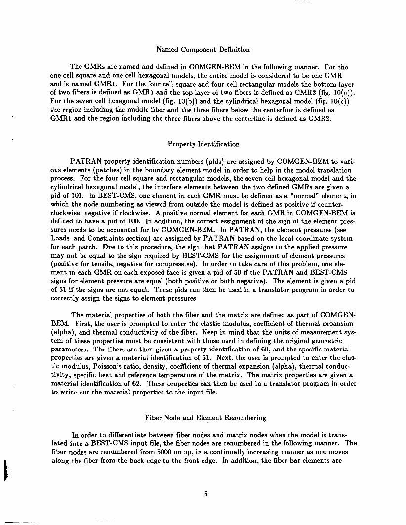
The GMRs are named and defined in COMGEN-BEM in the following manner. For the one cell square and one cell hexagonal models, the entire model is considered to be one GMR and is named GMR1. For the four cell square and four cell rectangular models the bottom layer of two fibers is defined as GMRl and the top iayer of two fibers is defined as GMR2 (fig. lO(a)). For the seven cell hexagonal model (fig. 10(b)) and the cylindrical hexagonal model (fig. lO(c)) the region including the middle fiber and the three fibers below the centerline is defined as GMRl and the region including the three fibers above the centerline is defined as GMR2.

Property Identification

PATRAN property identification numbers (pids) are assigned by COMGEN-BEM to vari- ous elements (patches) in the boundary element model in order to help in the model translation process. For the four cell square and rectangular models, the seven cell hexagonal model and the cylindrical hexagonal model, the interface elements between the two defined GMRs are given a pid of 101. In BEST-CMS, one element in each GMR must be defined as a “normal” element, in which the node numbering as viewed from outside the model is defined as positive if counter- clockwise, negative if clockwise. A positive normal element for each GMR in COMGEN-BEM is defined to have a pid of 100. In addition, the correct assignment of the sign of the element pres- sures needs to be accounted for by COMGEN-BEM. In PATRAN, the element pressures (see Loads and Constraints section) are assigned by PATRAN based on the local coordinate system for each patch. Due to this procedure, the sign that PATRAN assigns to the applied pressure may not be equal to the sign required by BEST-CMS for the assignment of element pressures (positive for tensile, negative for compressive). In order to take care of this problem, one ele- ment in each GMR on each exposed face is given a pid of 50 if the PATRAN and BEST-CMS signs for element pressure are equal (both positive or both negative). The element is given a pid of 51 if the signs are not equal. These pids can then be used in a translator program in order to correctly assign the signs to element pressures.

The material properties of both the fiber and the matrix are defined as part of COMGEN- BEM. First, the user is prompted to enter the elastic modulus, coefficient of thermal expansion (alpha), and thermal conductivity of the fiber. Keep in mind that the units of measurement sys- tem of these properties must be consistent with those used in defining the original geometric parameters. The fibers are then given a property identification of 60, and the specific material properties are given a material identification of 61. Next, the user is prompted to enter the elas- tic modulus, Poisson’s ratio, density, coefficient of thermal expansion (alpha), thermal conduc- tivity, specific heat and reference temperature of the matrix. The matrix properties are given a material identification of 62. These properties can then be used in a translator program in order to write out the material properties to the input file.

Fiber Node and Element Renumbering

In order to differentiate between fiber nodes and matrix nodes when the model is trans- lated into a BEST-CMS input file, the fiber nodes are renumbered in the following manner. The fiber nodes are renumbered from 5000 on up, in a continually increasing manner as one moves along the fiber from the back edge to the front edge. In addition, the fiber bar elements are

5

renumbered from 1000 on up, to differentiate fiber elements from matrix elements in the node renumbering process.

Fiber Rotation

In COMGEN-BEM, it is possible to define nonzero fiber rotation angles for the various models. This capability is available for situations where the model thickness is greater than or equal to the model width (or the largest width parameter for hexagonal and cylindrical hexa- gonal models). However, in order to maintain accurate fiber volume fractions in the model, it is recommended that the fiber rotation angle be varied only if the model thickness is equal to or slightly greater than the model width. If the thickness is greater than the width, lower angles of rotation give better results. For the four cell square and rectangular models, the user can vary the fiber rotation angle in each fiber layer independently. In the other models, all of the fibers are rotated together.

The user is first prompted to indicate whether or not the fiber orientation angle is non- zero. For the four cell square and rectangular models, the prompt is given separately for the bottom ply and the top ply. If the orientation angle is to be nonzero, the user is prompted to enter the fiber orientation angle. The angle may range from -89” to 90”. The positive direc- tion of the rotation angle is indicated in figure 11.

Since the fiber (and its generated circumference) cannot be clipped in BEST-CMS and must fit entirely inside the outer surface, the rotated fiber is scaled in size such that the rotated fiber will fit inside the model. For the hexagonal and cylindrical hexagonal models, extra care is given to insure that the fibers will also fit in the vertical direction, since the height of the model varies across the width.

Loads and Constraints

The final step in the model generation process is the specifications of the loads and con- straints that are to be applied to the model. The available load types are element pressures/ tractions, nodal forces/tractions, nodal temperatures and nodal displacements. In boundary element analysis, the applied forces are traction forces and must be entered in units of weight/ length squared. The user is first prompted to indicate whether or not loads (or other boundary conditions) are to be applied to the model. If loads are to be added, the user is prompted to indicate the load type which is to be applied (“PRES”-element pressure, “F0RC”-nodal forces, “D1SP”-nodal displacement or “TEMP”-nodal temperatures).

Once the load type is entered, the user is then prompted to enter the face (or load plane) number to which the boundary condition is to be applied. Figure 12 shows the load plane con- ventions for the square and rectangular models, figure 13(a) shows the load plane conventions for the hexagonal models and figure 13(b) shows the load plane conventions for the cylindrical hexagonal models. Note that for the hexagonal models only the front and back faces can be loaded due to the irregular shape of the other edges of the model. Once the load plane number is defined, the user is then prompted to enter the load set number. This is an integer number which is used to differentiate between different applied loadings. In order to be sure that all of the boundary conditions are translated correctly to the input file, it is recommended that each applied load be given a unique load set number.

6

i

I .

If element pressure (“PRES”) is chosen as the load type, the user will be prompted to enter the normal pressure acting on the indicated face. At this time, only normal pressures are permitted. The user should enter the applied pressure as positive if the load is tensile, negative if the load is compressive. For nodal forces and displacements, the user should enter the mag- nitude of the load along the global x, y, and z directions when prompted (positive for along the positive axis, negative for the opposite direction). If the boundary condition in a part.iciilar direction is to be specified to be zero, zero (0 ) should be entered at the prompt. If no boundary condition is to be imposed in a particular direction, a blank (pressing the space bar and then enter) should be entered. For nodal temperatures, the temperature should be given in the prompt for the x direction boundary condition and blanks should be entered in the other two directions. Once the specific load is applied, the user is again asked if loads are to be applied. If more loads are to be applied, “Y” should be entered at the prompt, otherwise “N” should be entered.

EXECUTING COMGEN-BEM

To run COMGEN-BEM, first a file (STARTUP.PCL or its equivalent, depending on the computer system) needs to be created in the same directory as the program file with the fol- lowing statement:

!! INPUT COMGEN - BEM

where comgenbem.pc1 is the name of the program file. This startup file is examined when PATRAN is executed, and will compile the PCL program into PATRAN. PATRAN is executed by entering “PATRAN” at the operating system prompt, and entering the terminal device number when prompted. At the next prompt, the user should enter “GO” and specify that a new file is to be created.

Once inside PATRAN, COMGEN-BEM can be executed by entering the following com- mand at the prompt:

! combem()

which will cause the PCL program to be executed. If the user desires, the program execution can be included in the PATRAN main menu by entering the following statements in a file called PATUSER.EMN.

MENU COMGEN BEM

PCL ! combem() ITEM MESH GENERATION

To execute COMGEN-BEM in from menu choices the user only has to select the “COMGEN BEM” option from the main PATRAN menu, and select the “MESH GENERATION” option from the submenu.

Once the program is executed, the user input and model generation proceeds as described above. A sample session showing user input and computer responses is shown in the appendix. Once the program has completed executing, the model will be plotted onto the screen. At this point, the user can make any fine adjustments needed to the model, or go ahead and utilize a

7

translator program to convert the model information into a BEST-CMS (or other boundary ele- ment code) input file. For help with PATRAN, an on-line help system is available and is accessed by entering “HELP” and then proceeding through the information screens until the desired topic is encountered.

CONCLUDING REMARKS

The COMGEN-BEM code allows the creation of boundary element models for composite micromechanics through the entry of a few simple parameters by the user. This program also allows users with a minimal knowledge of PATRAN to create a fairly complicated boundary ele- ment model. In this manner, parametric studies can be quickly and easily conducted, with effort spent in the interpretation of results instead of the creation of boundary element models.

a

APPENDIX-COMGEN-BEM SAMPLE SESSION

The following example shows a sample COMGEN-BEM session. The sample shows the generation of a one cell square model with the loads and constraints applied as shown in fig- ure 14. User inputs are indented and in bold face in the example. This example starts up from the point after the program is executed (either from the PATRAN command line or from a PATRAN menu).

9

ENTER MODEL TYPE (SQU/HEX/CHX/RGL)

SQU

Enter 1 for 1 cell, 2 for 4 cell

1

YOU HAVE CHOSEN A 1 CELL SQU MODEL

IS THIS CORRECT (Y/N)

Y

PLEASE ENTER THE FIBER VOLUME RATIO

0.34

PLEASE ENTER THE FIBER DIAMETER

0.145

DO YOU WANT A CUBIC MODEL (Y/N)

Y

ENTER NUMBER OF ELEMENTS THROUGH THE THICKNESS

1

ENTER NUMBER OF ELEMENTS IN THE FOLLOWING DIRECTIONS (CASE2)

B:

2

C:

2

D:

2

B= 2 C= 2 D= 2

ARE THESE VALUES CORRECT (Y/N)

Y

ENTER NUMBER OF ELEMENTS PER FIBER/INSERT

1

INPUT FIBER MODULUS

393.Ei-06

10

I .

INPUT FIBER ALPHA

2.23-06

INPUT FIBER CONDUCTIVITY

0.806

INPUT MATRIX MODULUS

88.E-

INPUT MATRIX POISSON’S RATIO

0.32

INPUT MATRIX DENSITY

4.7613-06

INPUT MATRIX ALPHA

8.13-06

INPUT MATRIX CONDUCTIVITY

8.101E+03

INPUT MATRIX SPECIFIC HEAT

5.024Ei-08

INPUT MATRIX TEMPERATURE

70.0

IS PLY ORIENTATION NONZERO(Y/N)

Y

INPUT FIBER ORIENTATION ANGLE

30

DO YOU WISH TO ADD LOADS (Y/N)

Y

ENTER THE TYPE OF LOAD (PRES,FORC,DISP,TEMP)

PRES

WHAT PLANE IS TO BE LOADED

1

ENTER LOAD SET ID NUMBER

11

1

ENTER NORMAL PRESSURE ACTING ON INDICATED FACE

lo00

DO YOU WISH TO ADD LOADS (Y/N)

Y

ENTER THE TYPE OF LOAD (PRES,FORC,DISP,TEMP)

DISP

WHAT PLANE IS TO BE LOADED

2

ENTER LOAD SET ID NUMBER

2

ENTER MAGNITUDE IN X DIRECTION OR BLANK

0.0

ENTER MAGNITUDE IN Y DIRECTION OR BLANK

0.0

ENTER MAGNITUDE IN Z DIRECTION OR BLANK

0.0

DO YOU WISH TO ADD LOADS (Y/N)

N

REFERENCES

1. Melis, M.E.: COMGEN: A Computer Program for Generating Finite Element Models of Composite Materials at the Micro Level. NASA TM-102556, 1990.

2. PATRAN Plus, User Manual. Release 2.4. BDA Engineering, Costa Mesa, C-4, 1990.

3. PATRAN Command Language (PCL) Guide. Release 2.4. PDA Engineering, Costa Mesa, CA, 1989.

4. Banerjee, P.K., et al.: BEST-CMS User’s Manual. Version 2.0. Computational Engineering Mechanics Laboratory, Department of Civil Engineering, State University of New York at Buffalo, Buffalo, NY, 1991.

13

(a) One cell square model.

0 .

e . I

(b) Four cell square model.

a . 0 .

I I

(c) Four cell rectangular model.

Figure 1 .-Bask square models.

(a) One cell hexagonal model.

/-----7

/- (b) Seven cell hexagonal model.

0 0 0

(c) Cylindrical hexagonal model.

Figure 2.-Bask hexagonal models.

14

(a) One cell square model-case I . (a) Four cell square model-case 1.

(b) One cell square model-case 2.

Figure 3.-Topological layout for one cell square model.

(b) Four cell square model-case 2.

Figure 4.-Topological layout for four cell square model.

(a) One cell hexagonal model.

@) Seven cell hexagonal model.

Figure B.-Topological layout for hexagonal models. Flgure 5.-TopologIcal layout for four cell rectangular model.

16

I---B+C+

(a) Mesh density directions-case 1.

Figure 7.-Topological layout for cylindrical hexagonal model.

(b) Mesh density directions-case 2.

Figure 8.-Mesh density directions for square models.

17

I-----;+ (a) Hexagonal models.

(b) Rectangular models.

Figure 9.-Mesh density directlons for hexagonal, cyllndrlcal hexagonal and rectangular models.

(a) Four cell square and four cell rectangular models.

4' i \ G M R 2

\

(b) Seven cell hexagonal model.

/---

-. .. '---I

(c) Cylindrlcal hexagonal model.

Flgure 1 O.-Modeling region deflnltions.

Model centerline

L

Figure 11 .-Positive direction for fiber rotation angle.

L .

,-

Figure 12.-Load plane conventions for square and rectangular models.

19

I

(a) One and seven cell hexagonal models.

(b) Cylindrical hexagonal model.

Figure 13.-Load plane conventions for hexagonal models.

ZL-1; c- ' z 3 Flgure 14.-Load and COnStralntS aPPlled to sample problem.

20

REPORT DOCUMENTATION PAGE

I I

I. TITLE AND SUBTITLE

COMGEN-BEM: Boundary Element Model Generation for Composite Materials Micromechanical Analysis

Form Approved OMB NO. 0704-0188

i. AUTHOR(S)

Robert K. Goldherg

I. AGENCY USE ONLY (Leave blank)

1. PERFORMING ORGANIZATION NAME(S) AND ADDRESS(ES)

2. REPORT DATE 3. REPORT TYPE AND DATES COVERED

March 1992 Technical Memorandum

National Aeronautics and Space Administration Lewis Research Center Cleveland, Ohio 44135-3191

128- DlSTRlBUTlON/AVAlLABlLlTY STATEMENT

3. SPONSORING/MONITORING AGENCY NAMES(S) AND ADDRESS(ES)

12b. DISTRIBUTION CODE

National Aeronautics and Space Administration Washington, D.C. 20546-0001

Boundary element mcthod; Composite materials; Preprocessing

17. SECURITY CLASSIFICATION 18. SECURITY CLASSIFICATION 19. SECURlTy CLASSIFICATION OF REPORT OF THIS PAGE OF ABSTRACT

Unclassified Unclassified Unclassified

11. SUPPLEMENTARY NOTES

Responsible person Robert K. Goldberg, (21 6) 433-3330.

27

A03 16. PRICE CODE

20. LIMITATION OF ABSTRACT

5. FUNDING NUMBERS

WU -5 1 0-01 -50

8. PERFORMING ORGANIZATION REPORT NUMBER

E-6871

10. SPONSORlNGlMONlTORlNG AGENCY REPORT NUMBER

NASA TM- 105548

I I I NSN 7540-01 -280-5500 Standard Form 298 (Rev. 2-89)

prescribed by ANSI Std 239-18 298-102

~

Unclassified -Unlimited Subject Category 39

13. ABSTRACT (Maximum 200 words)

COMGEN-BEM ( a m p o s i t e Model mera t ion-Boundary Element Method) is a program developed in PATRAN Command Language (PCL) which generates boundary element models of continuous fiber composites at thc micromechanical (constituent) scale. Based on the entry of a few simple parameters such as fihcr volume fraction and fiber diameter the model geometry and boundary clement model arc generated. In addition, various mesh densities, material properties, fiber orientation angles, loads and boundary conditions can he specified. The gener- ated model can then be translated to a format consistcnt with a boundary element analysis code such as BEST-CMS.

14. SUBJECT TERMS 115. NUMBER OF PAGES