NASA-CR-202063/

/ /_ _.:/ , V L..i"

0 c-IF-_

NASA TREETOPS

FINAL REPORT

Prepared by:

Oakwood College/Dynamic Concepts, Inc.June 1996

CONTRACT NAS8-40194

https://ntrs.nasa.gov/search.jsp?R=19960047074 2020-02-23T08:32:22+00:00Z

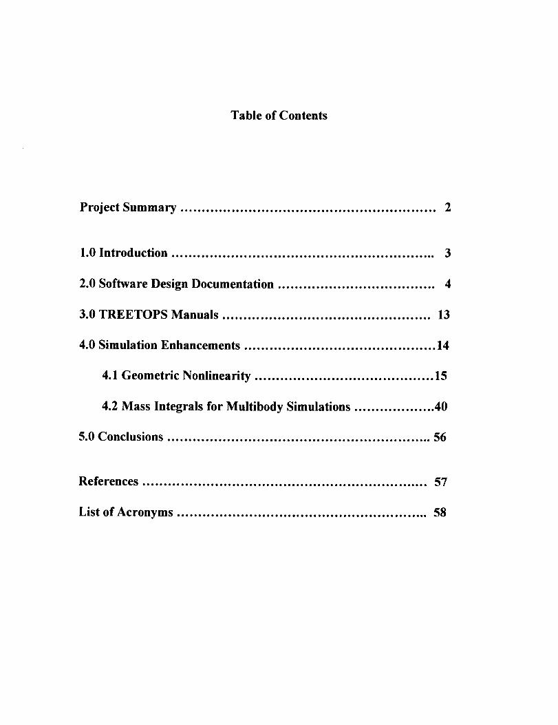
Table of Contents

Project Summary ............................................................ 2

1.0 Introduction .............................................................. 3

2.0 Software Design Documentation ..................................... 4

3.0 TREETOPS Manuals ................................................. 13

4.0 Simulation Enhancements ............................................. 14

4.1 Geometric Nonlinearity .......................................... 15

4.2 Mass Integrals for Multibody Simulations ................... 40

5.0 Conclusions .............................................................. 56

References ................................................................... 57

List of Acronyms ........................................................... 58

Project Summary

Under the provisions of contract number NAS8-40194, which was entitled

"TREETOPS Structural Dynamics and Controls Simulation System Upgrade', Oakwood

College contracted to produce an upgrade to the existing TREETOPS suite of analysis

tools. This suite includes the main simulation program, TREETOPS, two interactive

preprocessors, TREESET and TREEFLX, an interactive post processor, TREEPLOT, and

an adjunct program, TREESEL.

The capability of the TREETOPS simulation package was extended by providing

the ability to handle geometrically nonlinear problems through the use of a specially

designed "User Controller'. Software for computing the modal integrals from any finite

element code (e.g., NASTRAN, ANSYS, etc.) was developed in two forms--Fortran source

code and a MATLAB script file.

A "Software Design Document", which provides descriptions of the argument lists

and internal variables for each subroutine in the TREETOPS suite, was established.

Additionally, installation guides for both DOS and UNIX platforms were developed. Finally,

updated User's Manuals, as well as a Theory Manual, were generated under this contract.

2

1.0 Introduction

The TREETOPS simulation package is a multibody dynamics tool capable of

formulating and integrating the equations of motion for a wide variety of aerospace and

mechanical systems. Special attention to implementation and integration of controllers

(passive and/or active) into the state equations was paid in the initial formulation of the

code--which sets it apart form other mechanical dynamics codes.

Over time, certain deficiencies and limitations in the TREETOPS code have been

noted in the user community. Among these deficiencies was a lack of software control

documents, limitations to geometrically linear response regimes, and a lack of user friendly

modal integral tools. NASA contract number NAS8-40194 was established to address

these concerns.

This report will detail the activities undertaken in pursuit of the goals established

for contract NAS8-40194. The Software Design Document, not included here for the sake

of brevity, will be discussed in Section 2 of this report. The updates and additions to the

TREETOPS Manuals are presented in Section 3. Section 4 details the simulation

enhancements_ich include the addition of geometric stiffening to the code as well as

the development of user-friendly modal integral software tools. Section 5 will conclude this

report.

3

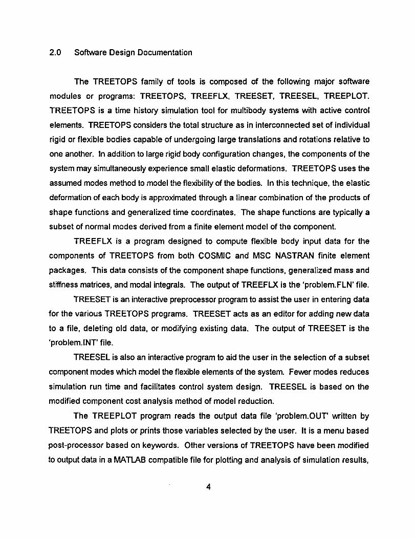
2.0 Software Design Documentation

The TREETOPS family of tools is composed of the following major software

modules or programs: TREETOPS, TREEFLX, TREESET, TREESEL, TREEPLOT.

TREETOPS is a time history simulation tool for multibody systems with active control

elements. TREETOPS considers the total structure as in interconnected set of individual

rigid or flexible bodies capable of undergoing large translations and rotations relative to

one another. In addition to large rigid body configuration changes, the components of the

system may simultaneously experience small elastic deformations. TREETOPS uses the

assumed modes method to model the flexibility of the bodies. In this technique, the elastic

deformation of each body is approximated through a linear combination of the products of

shape functions and generalized time coordinates. The shape functions are typically a

subset of normal modes derived from a finite element model of the component.

TREEFLX is a program designed to compute flexible body input data for the

components of TREETOPS from both COSMIC and MSC NASTRAN finite element

packages. This data consists of the component shape functions, generalized mass and

stiffness matrices, and modal integrals. The output of TREEFLX is the 'problem.FLN' file.

TREESET is an interactive preprocessor program to assist the user in entering data

for the various TREETOPS programs. TREESET acts as an editor for adding new data

to a file, deleting old data, or modifying existing data. The output of TREESET is the

'problem.INT' file.

TREESEL is also an interactive program to aid the user in the selection of a subset

component modes which model the flexible elements of the system. Fewer modes reduces

simulation run time and facilitates control system design. TREESEL is based on the

modified component cost analysis method of model reduction.

The TREEPLOT program reads the output data file 'problem.OUT' written by

TREETOPS and plots or prints those variables selected by the user. It is a menu based

post-processor based on keywords. Other versions of TREETOPS have been modified

to output data in a MATLAB compatible file for plotting and analysis of simulation results,

4

thereby minimizing the use of TREEPLOT.

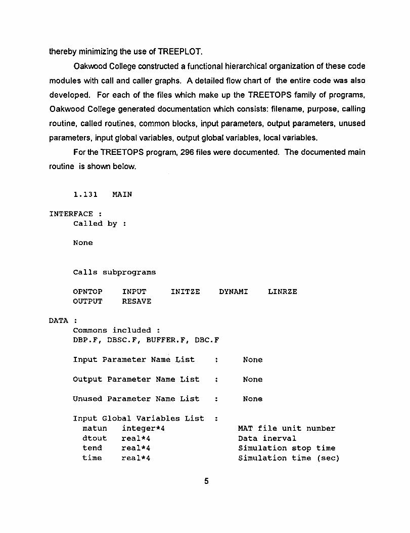
Oakwood College constructed a functional hierarchical organization of these code

modules with call and caller graphs. A detailed flow chart of the entire code was also

developed. For each of the files which make up the TREETOPS family of programs,

Oakwood College generated documentation which consists: filename, purpose, calling

routine, called routines, common blocks, input parameters, output parameters, unused

parameters, input global variables, output global variables, local variables.

For the TREETOPS program, 296 files were documented. The documented main

routine is shown below.

1.13 1 MAIN

INTERFACE :

Called by :

None

DATA

Calls subprograms

OPNTOP INPUT INITZE DYNAMI LINRZE

OUTPUT RESAVE

Commons included :

DBP.F, DBSC.F, BUFFER.F, DBC.F

Input Parameter Name List None

Output Parameter Name List : None

Unused Parameter Name List : None

Input Global Variables List

matun integer*4

dtout real*4

tend real*4

time real*4

MAT file unit number

Data inerval

Simulation stop time

Simulation time (sec)

5

tlin real*4

linearization option,

data

(is

Time used in the

=0 if L is chosen, =TEND + 1 for Z and N

toend real*4

plotting, =TEND

tostrt real*4

usually equal to 0)

End of the time interval for

Start time for data plotting

Output Global Variables List : None

DESCRIPTION :

Found in file :

maintops.for

Purpose :

This is the main program of treetops and it calls seven other

major

subprograms to perform the task of TREETOP software. The

subprograms

are:

-- OPNTOP

and

-- INPUT

calling

-- INITZE

-- DYNAMI

vector.

-- LINRZE

-- OUTPUT

Both

: Open necessary files to support TREETOPS input

output data.

: Drive the data input function for TREETOPS by

the appropriate input routines.

: Initialize the simulation and perform initial

computation of simulation data.

: Execute the simulation dynamics by performing

integration and propagation of the system state

: Generate the linearized system dynamics.

: Store simulation output data in two data files.

files contain identical information, but one file is

formated and the other is unformated.

-- RESAVE : Outputs event information at the end of the

simulation.

8

For the TREEFLX program, 119 files were documented. The documentation for the

main routine of TREEFLX is as follows.

3.118 TREFLX

INTERFACE ."

Called by :

None

Calls subprograms :

DEDAMP ERRWRT EXTDAT MEMCHK NODCHK

OPNFACE

RDAGMT RDNAST RDRTMD TMCALC WRTFLX

DATA ."

Commons included

PARI.F PAR2.F

Input Parameter Name List

Output Parameter Name List :

Unused Parameter Name List :

Input Global Variables List :

augy

bbid

bbnu

flxbnm

flxid

nmodbj

nnodbj

nuflbd

dammth

redmth

error

doesex

integer*4(pnbb)

integer*4

integer*4

integer*4 (pnbb)

integer*4 (pnbb)

integer*4 (pnbb)

integer*4(pnbb)

integer*4

character*2(pnbb)

character*l(pnbb)

logical*4

logical*4

Output Global Variables List :

None

None

None

OPNDAF

7

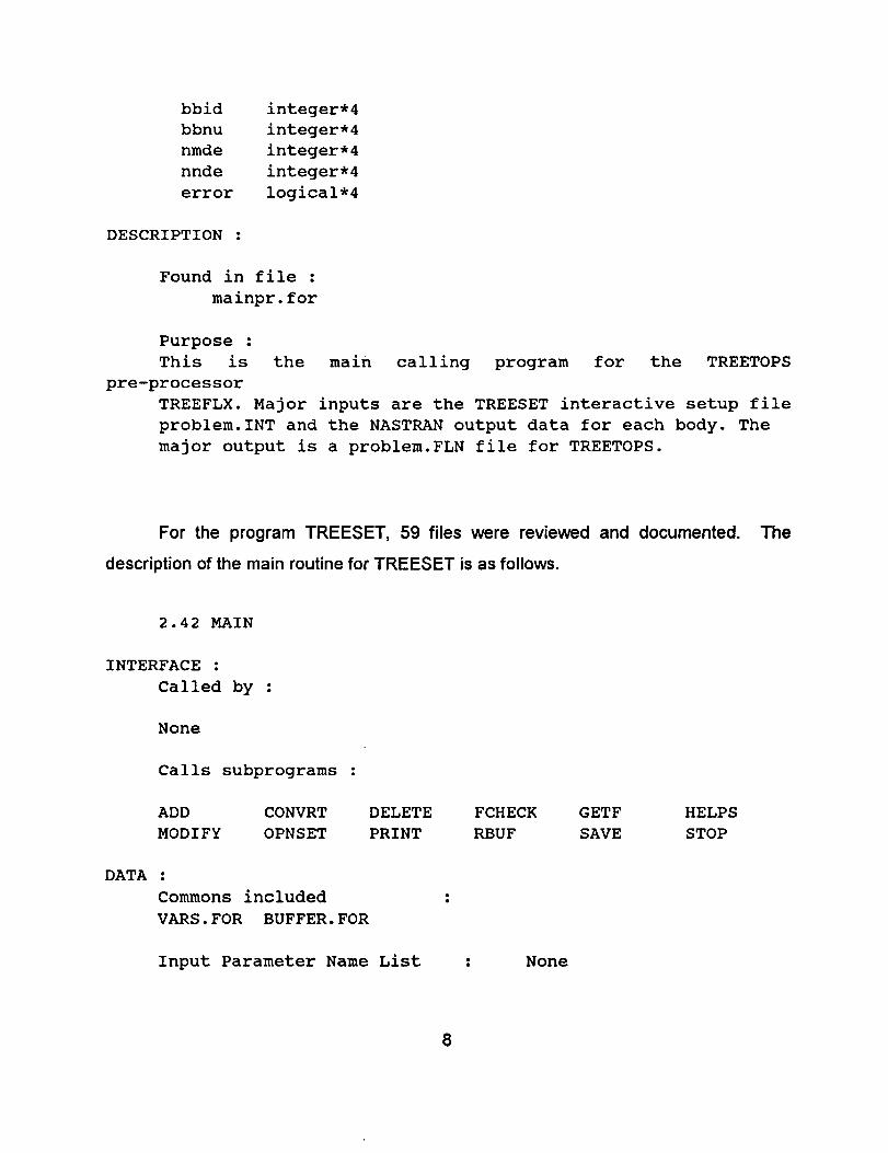
bbid integer*4

bbnu integer*4

nmde integer*4

nnde integer*4

error logical*4

DESCRIPTION :

Found in file :

mainpr.for

Purpose :

This is the main calling program for the TREETOPS

pre-processor

TREEFLX. Major inputs are the TREESET interactive setup file

problem. INT and the NASTRAN output data for each body. The

major output is a problem. FLN file for TREETOPS.

For the program TREESET, 59 files were reviewed and documented. The

description of the main routine for TREESET is as follows.

2.42 MAIN

INTERFACE :

Called by :

None

Calls subprograms :

ADD CONVRT DELETE FCHECK GETF HELPS

MODIFY OPNSET PRINT RBUF SAVE STOP

DATA :

Commons included

VARS.FOR BUFFER.FOR

Input Parameter Name List : None

8

Output Parameter Name List : None

Unused Parameter Name List : None

Input Global Variables List

revno integer*4

revdat character*8

ifunct integer*4

Output Global Variables List :

revno integer*4

revdat character*8

DESCRIPTION :

Found in file :

main.for

Purpose :

This is the main routine for TREETOPS pre-processor TREESET.

The output of TREESET is the problem. INT file which is read

by TREETOPS.

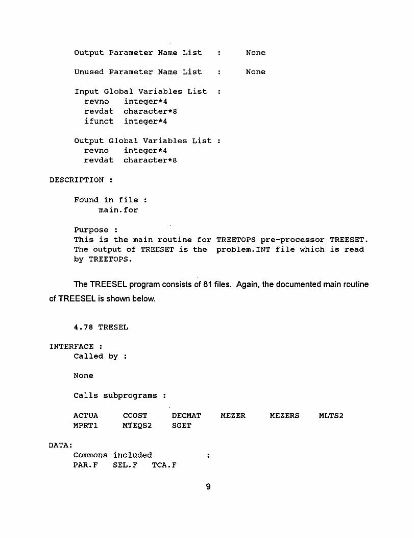
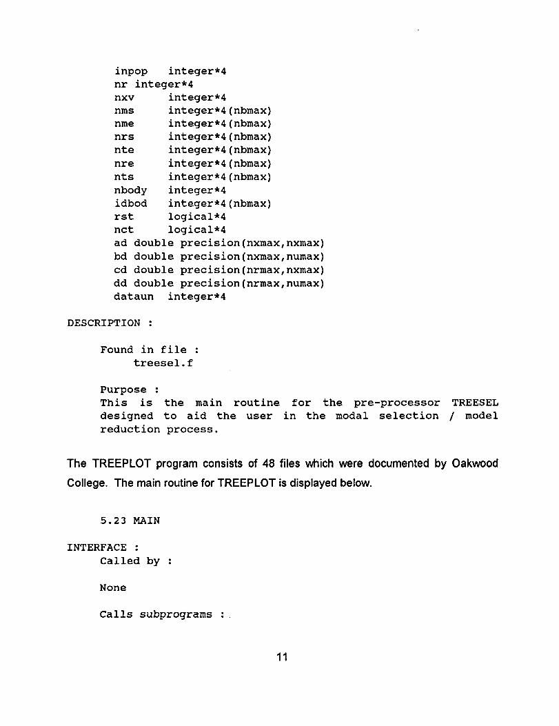
The TREESEL program consists of 81 files. Again, the documented main routine

of TREESEL is shown below.

4.78 TRESEL

INTERFACE :

DATA:

Called by :

None

Calls subprograms :

ACTUA CCOST

MPRTI MTEQS2

DECMAT MEZER MEZERS MLTS2

SGET

Commons included

PAR.F SEL.F TCA.F

9

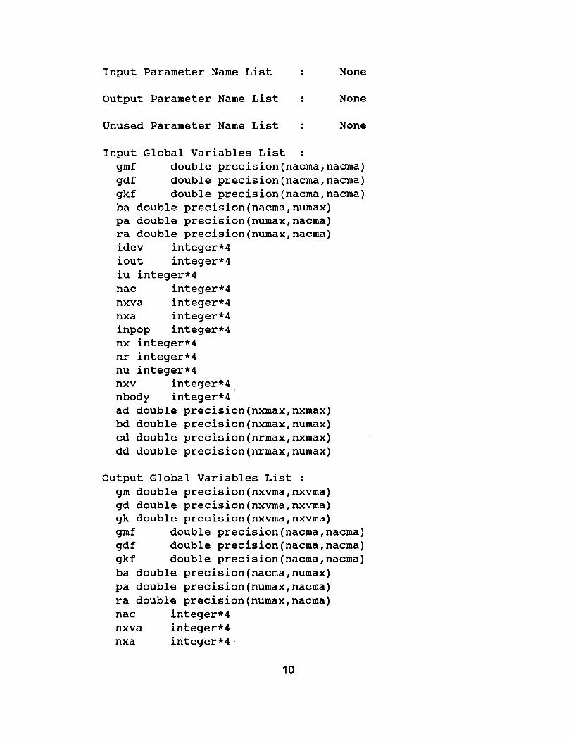
Input Parameter Name List : None

Output Parameter Name List : None

Unused Parameter Name List : None

Input Global Variables List :

gmf double precision(nacma,nacma)

gdf double precision(nacma,nacma)

gkf double precision(nacma,nacma)

ba double precision(nacma,numax)

pa double precision(numax,nacma)

ra double precision(numax,nacma)

idev integer*4

iout integer*4

iu integer*4

nac integer*4

nxva integer*4

nxa integer*4

inpop integer*4

nx integer*4

nr integer*4

nu integer*4

nxv integer*4

nbody integer*4

ad double precision(nxmax,nxmax)

bd double precision(nxmax,numax)

cd double precision(nrmax,nxmax)

dd double precision(nrmax,numax)

Output Global Variables List :

gm double precision(nxvma,nxvma)

gd double precision(nxvma,nxvma)

gk double precision(nxvma,nxvma)

gmf double precision(nacma,nacma)

gdf double precision(nacma,nacma)

gkf double precision(nacma,nacma)

ba double precision(nacma,numax)

pa double precision(numax,nacma)

ra double precision(numax,nacma)

nac integer*4

nxva integer*4

nxa integer*4.

I0

inpop integer*4

nr integer*4

nxv integer*4

nms integer*4(nbmax)

nme integer*4(nbmax)

nrs integer*4(nbmax)

nte integer*4(nbmax)

nre integer*4(nbmax)

nts integer*4(nbmax)

nbody integer*4

idbod integer*4(nbmax)

rst logical*4

nct logical*4

ad double precision(nxmax,nxmax)

bd double precision(nxmax,numax)

cd double precision(nrmax,nxmax)

dd double precision(nrmax,numax)

dataun integer*4

DESCRIPTION :

Found in file :

treesel.f

Purpose :

This is the main routine for the pre-processor TREESEL

designed to aid the user in the modal selection / model

reduction process.

The TREEPLOT program consists of 48 files which were documented by Oakwood

College. The main routine for TREEPLOT is displayed below.

5.23 MAIN

INTERFACE :

Called by :

None

Calls subprograms :

11

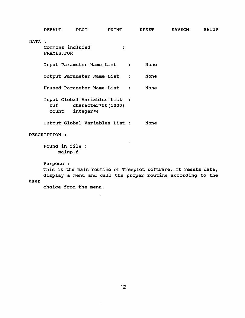
DEFALT PLOT PRINT

DATA :

Commons included

FRAMES.FOR

Input Parameter Name List

Output Parameter Name List :

Unused Parameter Name List :

Input Global Variables List :

buf character*50(1000)

count integer*4

Output Global Variables List :

DESCRIPTION :

user

RESET SAVECM SETUP

: None

None

None

None

Found in file :

mainp.f

Purpose :

This is the main routine of Treeplot software. It resets data,

display a menu and call the proper routine according to the

choice from the menu.

12

3.0 TREETOPS Manuals

Revised TREETOPS theoretical and user manuals were developed by Oakwood

College under this effort. The User's Manual was prepared in a format approved by the

NASA COTR to allow the user to exercise the TREETOPS package. Additionally, the

User's Manual modified to correct current deficiencies and changes. The manual

presents detailed information necessary to use all options available in the program.

Various examples which cover the main features were included as well as trouble shooting

information and software compilation and installation notes. Example problems were

worked in the manual and supplied on disk to validate the operation of TREETOPS.

The current TREETOPS Theory Manual was reviewed and revised. Parts of the

TREETOPS and CONTOPS User's Manuals were included in the revised Theory Manual

to provide background on how TREETOPS works. The notation within the Theory Manual

was changed to be consistent. A section on geometric non-linearities was added to the

manual.

13

4.0 Simulation Enhancements

Under this contract, a general procedure for incorporating geometric stiffening into

the TREETOPS simulation package was developed. An algorithm, FORTRAN program,

and MATLAB M file were also developed to compute the modal integrals and other data

required for the 'problem.FLX' file. These accomplishments are discussed in Sections 4.1

and 4.2 through documents previously distributed to NASA and reprinted here in entirety.

14

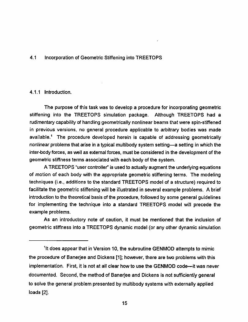
4.1 Incorporation of Geometric Stiffening into TREETOPS

4.1.1 Introduction.

The purpose of this task was to develop a procedure for incorporating geometric

stiffening into the TREETOPS simulation package. Although TREETOPS had a

rudimentary capability of handling geometrically nonlinear beams that were spin-stiffened

in previous versions, no general procedure applicable to arbitrary bodies was made

available. 1 The procedure developed herein is capable of addressing geometrically

nonlinear problems that arise in a typical multibody system settingma setting in which the

inter-body forces, as well as external forces, must be considered in the development of the

geometric stiffness terms associated with each body of the system.

A TREETOPS "user controller" is used to actually augment the underlying equations

of motion of each body with the appropriate geometric stiffening terms. The modeling

techniques (i.e., additions to the standard TREETOPS model of a structure) required to

facilitate the geometric stiffening will be illustrated in several example problems. A brief

introduction to the theoretical basis of the procedure, followed by some general guidelines

for implementing the technique into a standard TREETOPS model will precede the

example problems.

As an introductory note of caution, it must be mentioned that the inclusion of

geometric stiffness into a TREETOPS dynamic model (or any other dynamic simulation

lit does appear that in Version 10, the subroutine GENMOD attempts to mimic

the procedure of Banerjee and Dickens [1]; however, there are two problems with this

implementation. First, it is not at all clear how to use the GENMOD code---it was never

documented. Second, the method of Banerjee and Dickens is not sufficiently general

to solve the general problem presented by multibody systems with externally applied

loads [2].

15

package) is generally a task that should be undertaken only by individuals with a relatively

high degree of experience in both TREETOPS modeling and the finite element method.

Whereas the required additions to the TREETOPS model ( <...>.int and <...>.fix files) are

straightforward, the preparation of the required generalized geometric stiffness matrices

is somewhat laborious and typically requires the use of a finite element package (e.g.,

NASTRAN) capable of solving geometrically nonlinear problems.

4.1.2 Brief Theoretical Background.

This section presents a synopsis of the underlying mechanics associated with the

inclusion of geometric stiffness into TREETOPS. A complete derivation of the associated

nonlinear equations can be found in Reference [1]. For the sake of clarity, the inclusion

of geometric stiffness in the =standard" structural dynamics problem, i.e.,

M_ + Kx = F (1)

will be used to develop the salient features of the new TREETOPS procedures. =

stiffness matrix in the above equation can be broken down into two parts,

The

K = K L + K o (2)

where K. is the usual linear stiffness matrix and K o is the geometric stiffness matrix.

The geometric stiffness matrix is a function of the internal (stress) loads acting in

the body (i.e., K o = Ko(o)). For linear structures, the internal loads are a linear function

of the applied loads. In other words, o = o(f_.,., f_). If we make the assumption that the

inertial loads' contribution to K o is due to the rigid body motions of the body in question,

then the inertial loads can be developed directly from Newton's 2nd Law and Euler's

equation for the lumped mass case, e.g.,

= Reference [1] contains the analogous development for the fully nonlinear

multibody equations of motion; however, the simpler development presented herein

should allow the user sufficient depth of knowledge to address a wide range of

geometrically nonlinear problems.

16

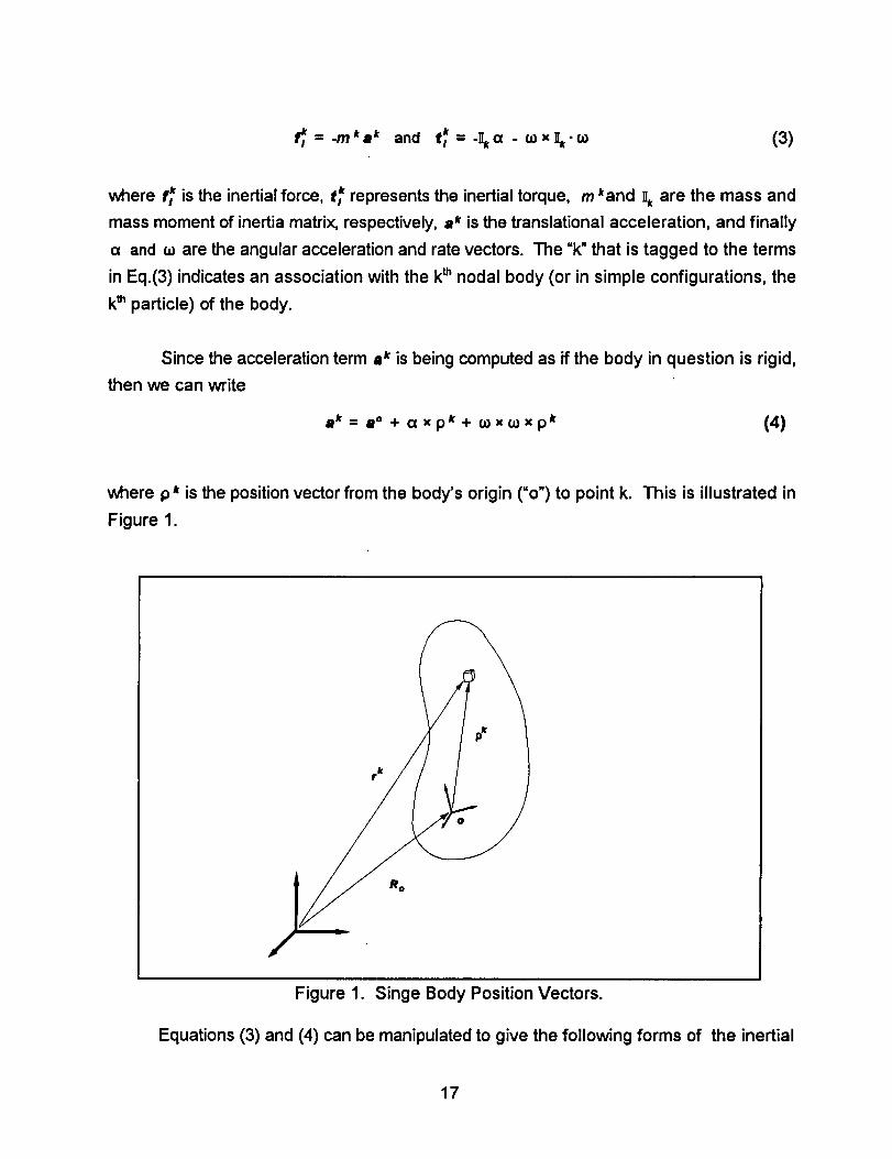
: -m'a* and tl* = -]_a - £oxl,-_o (3)

where f_ is the inertial force, t_' represents the inertial torque, m *and _, are the mass and

mass moment of inertia matrix, respectively, a s is the translational acceleration, and finally

a and ¢o are the angular acceleration and rate vectors. The "k" that is tagged to the terms

in Eq.(3) indicates an association with the kth nodal body (or in simple configurations, the

kth particle) of the body.

Since the acceleration term a s is being computed as if the body in question is rigid,

then we can write

aS = @o + G xpk+ O) XO)Xp k (4)

where p* is the position vector from the body's origin ("o") to point k. This is illustrated in

Figure 1.

Figure 1. Singe Body Position Vectors.

Equations (3) and (4) can be manipulated to give the following forms of the inertial

17

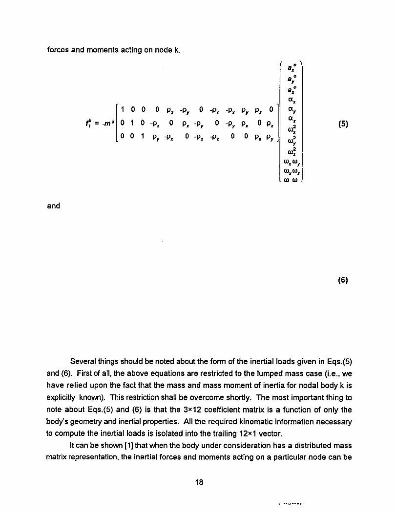
forces and moments acting on node k.

r_l " -m k

1 0 0 0 p= -py 0 -Px -Px Py Pz 0

0 1 0 "Pz 0 Px-Py 0 -py Px 0 Pz

0 0 1 Py-Px 0-Pz -Pz 0 0 Px Py

a,"a x

ay

Qz (5)

and

(6)

Several things should be noted about the form of the inertial loads given in Eqs.(5)

and (6). First of all, the above equations are restricted to the lumped mass case (i.e., we

have relied upon the fact that the mass and mass moment of inertia for nodal body k is

explicitly known). This restriction shall be overcome shortly. The most important thing to

note about Eqs.(5) and (6) is that the 3x12 coefficient matrix is a function of only the

body's geometry and inertial properties. All the required kinematic information necessary

to compute the inertial loads is isolated into the trailing 12xl vector.

It can be shown [1] that when the body under consideration has a distributed mass

matrix representation, the inertial forces and moments acting on a particular node can be

18

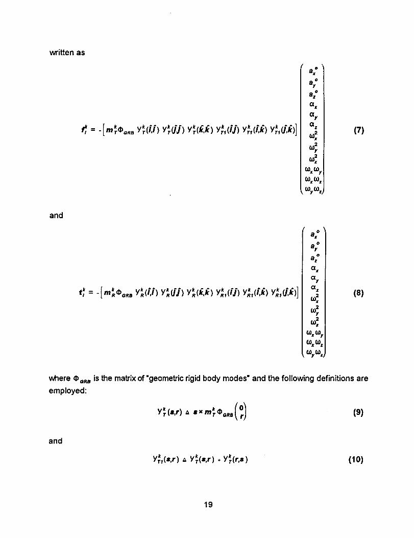
written as

ax"

a."G x

Gy

G z

<

20.1z

0) x (JOy

oJxo)z

(7)

and

G x

Gy

G z

<

<00,%%%

,%%,

(8)

where _ e_,

employed:

is the matrix of "geometric rigid body modes" and the following definitions are

Y_(=,r) = SXmreo_ a (9)

and

Yrk,(s,r) = Y_(s,r)+ Ykr(r,s ) (10)

19

The Y_ (s,r)are Y*,I (s,r)terms are defined analogously.

The form of Eqs.(7) and (8) appear somewhat unwieldy, but in fact the procedures

followed to compute the inertial loads are straightforward. It should also be noted that

Eqs.(7) and (8), which are sufficiently general to address the distributed mass case,

collapse to the simpler forms of Eqs.(5) and (6) when a lumped mass representation is

assumed.

For brevity, Eqs.(7) and (8) can be stacked and written as

(11)

* 6xl vector, F_ is a 6x12 coefficient matrix, and A_ is the 12xl vector ofwhere f_,t is a

kinematic variables. The above equation can be generalized to compute the inertial load

vectors for the entire body (i.e., all nodes, not just node k) by essentially =stacking up" all

of the nodal inertial loads. This process leads to the following equation,

_',_ = F_. A, (12)_=1 n=12 12=1

where f_,_t is the nxl vector of inertial loads acting on the body, F_ is a nx12 coefficient

matrix, and A, is the usual 12xl vector of kinematic variables. At this point, it is useful to

think of the F_ matrix as simply the container for 12 nxl inertial load vectors--each

associated with a particular kinematic quantity contained in the .4_ vector.

We are now in a position to expand the geometric stiffness matrix into a form that

will be appropriate for introduction into the dynamic simulation. Since the K o matrix is

function of the loads acting on the body (inertial and external), it can be expanded into the

following form

K o = Ke(f_ + f..,) = Ke(f_,,) + Ke(f., ) (13)

By substituting Eq.(12) into Eq.(13), the geometric stiffness matrix that accounts for the

inertial loading (i.e., the "motion stiffness') can be written as

20

where the Fl(i ) vectors are simply columns of the F I matrix. Note that there are 12

geometric stiffness matrices associated with the inertial loads, namely K o (F, (i)), I = 1,12.

The geometric stiffening due to external loading can be expanded in a manner

similar to the inertial loading, i.e.,

K e (f,,,) = K= _ F,=t(i). f,x,(i ) = K o (F=t (i)). f,,(i ) (151I"t I

The external loads in the above equation have been expanded into ne =locator" vectors

(F,,(i)) and associated magnitudes (f,=t(i)). It should be noted that there are ne

geometric stiffness matrices, each associated with one of the ne external loads. For the

multibody case, all inter-body forces acting through joints or hinges are considered

externally applied forces as far as the geometric stiffening is concerned.

By expanding the K o matrix into the forms represented by Eqs.(14) and (15), the

time-varying nature of K o is isolated to the A_(i) = Aj(i,t) and f,t(i) = f,,t(i,t) terms. This

allows the 12 K o (F_(i)) and ne K o (F,=t (i)) matrices to be computed in advance of any

simulation effort. Any finite element code capable of producing geometric stiffness

matrices should be able to provide the required data.

As is typical in the consideration of flexibility of multibody systems, we will consider

the flexibility of any particular body to be expressed as a linear combination of shape

vectors (e.g., modeshapes). Hence, a need arises for the calculation of generalized or

modal stiffness matrices. For TREETOPS, the linear modal stiffness matrix is input

through the <...>.fix file. The modal geometric stiffness terms, which are defined below,

are read into the user controller wherein they are multiplied by the appropriate modal

coordinates. Elements of the modal geometric stiffness matrices are defined as:

K'=,_qj A 4)_Ke(Fl(i))dp 1 (16)

and

TK _2_q1 A (l)'qKe (F,=,(i)) (1)1 (17)

where ¢)/ is the j_ modeshape vector. The modal force associated with the geometric

stiffening terms can now be written as

21

._r= K_,°Al(i,t ) + _ K I "o2"r,.t(I,t)Ll'1 1-1

n (18)

where q is the vector of modal coordinates. The calculation of the modal force terms

given in Eq.(18) is performed in the user controller. This will be demonstrated in the

example problems presented later in this report.

4.1.3 General Implementation Discussion.

As a prerequisite to actually incorporating the geometrically nonlinear capabilities

into TREETOPS for a particular dynamic system, the analyst should go through a mental

screening process to determine the necessity of the nonlinear analysis. The essence of

this screening test is the question, "Is a geometrically nonlinear response likely from this

system?" In general, this question is very difficult to answer. For relatively stiff structures,

geometrically nonlinear responses are uncommon. However, there are several situations

in which geometric stiffening may play a significant role in the system response. For

rotating structures, if the spin rate approaches (or exceeds) the first natural frequency of

the structure, then the geometric stiffness terms are necessary in the analysis. For

structures constructed from beams and plates, compressive loading in the body can

significantly modify the stiffness of the structure. When the user finds himself in the

unfortunate position of not knowing whether or not to expect a geometrically nonlinear

response, the inclusion of the nonlinear stiffening terms is the safest course to follow

despite the not insigficant effort involved.

The initial step in building the geometrically nonlinear TREETOPS model is to

decide which of the bodies in the system require the geometric stiffening terms. Consider

a satellite/antenna system during a slewing manuever. Since the core body (satellite) is

likely to be much stiffer than the antenna, only the antenna body would be considered

likely to produce a geometrically nonlinear response. Hence, the geometric stiffening

terms utilized in Eq.(18) need only be computed for the antenna body, not the core body.

The overall procedure for integrating the geometric stiffening terms into TREETOPS

is presented in Figure 2. For each body requiring geometric stiffening terms, the first step

in the analysis is to compute the F_(i) inertial load vectors. A Matlab m-file (fimake5.m)

has been created which will produce these inertial load vectors. The initial portion of this

Matlab function is shown below.

22

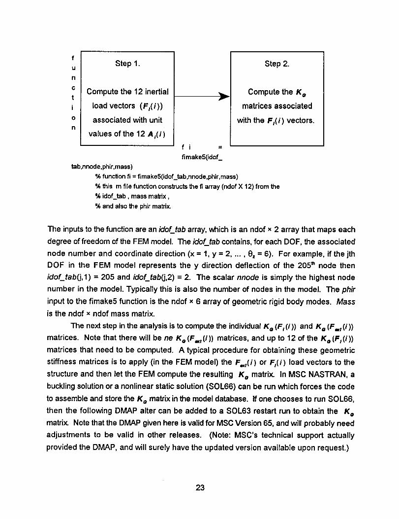
Step 1.

Compute the 12 inertial

load vectors (F_(i))

associated with unit

values of the 12 A_(i)

f

f i =

fimakeS(idof_

Step 2.

Compute the K o

matrices associated

with the F_(i) vectors.

tab,nnode,phir,mass)

% function fi = fimake5(idof_tab,nnode,phir,mass)

% this m file function constructs the fi array (ndof X 12) from the

% idof_tab, mass matrix,

% and also the phir matrix.

The inputs to the function are an idof_tab array, which is an ndof x 2 array that maps each

degree of freedom of the FEM model. The idof_tab contains, for each DOF, the associated

node number and coordinate direction (x = 1, y = 2 ..... ez = 6). For example, if the jth

DOF in the FEM model represents the y direction deflection of the 205 = node then

idof_tabG,1) = 205 and idof_tab_j,2) = 2. The scalar nnode is simply the highest node

number in the model. Typically this is also the number of nodes in the model. The phir

input to the fimake5 function is the ndof x 6 array of geometric rigid body modes. Mass

is the ndof x ndof mass matrix.

The next step in the analysis is to compute the individual !( e (Fl(i)) and K o (F=t(i))

matrices. Note that there will be ne K o (F,t (i)) matrices, and up to 12 of the K o (F_ (i))

matrices that need to be computed. A typical procedure for obtaining these geometric

stiffness matrices is to apply (in the FEM model) the F,t(i ) or F,(i) load vectors to the

structure and then let the FEM compute the resulting K o matrix. In MSC NASTRAN, a

buckling solution or a nonlinear static solution (SOL66) can be run which forces the code

to assemble and store the K o matrix in the model database. If one chooses to run SOL66,

then the following DMAP alter can be added to a SOL63 restart run to obtain the K o

matrix. Note that the DMAP given here is valid for MSC Version 65, and will probably need

adjustments to be valid in other releases. (Note: MSC's technical support actually

provided the DMAP, and will surely have the updated version available upon request.)

23

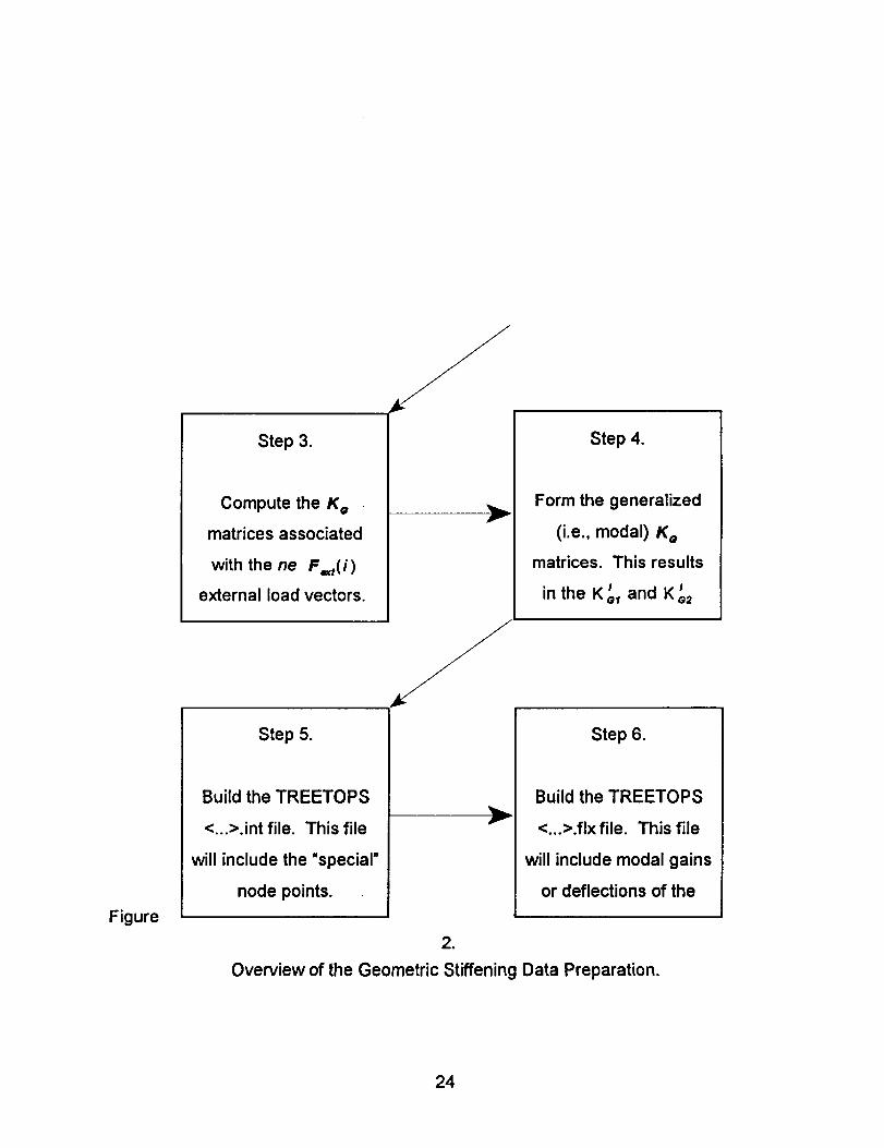
Figure

Step 3.

Compute the K o

matrices associated

with the ne F =t( i )

external load vectors.

Step 5.

Build the TREETOPS

<...>.int file. This file

will include the "special"

node points.

Step 4.

Form the generalized

(i.e., modal) K o

matrices. This results

in theKol_ andK_2

Step 6.

Build the TREETOPS

<...>.fix file. This file

will include modal gains

or deflections of the

,

Overview of the Geometric Stiffening Data Preparation.

24

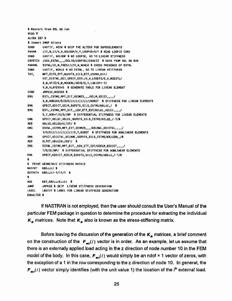
$ Restart from SOL 66 run

READ 9

ALTER 287 $

$ Insert DMAP Atters

COND

PARAM

COND

DBFETCH

PARAML

COND

TA1,

COND

EMG

EMA

EMG

EMA

ADD

EMG

EMA

ADD

EMG

EMA

$

$ PRINT GEOMETRIC STIFFNESS MATRIX

NATPRT KBDJJ// $

OUTPUT4 KBDJJ//-1/11/1 $

$

ADD KB1,KBDJJ/KJJZ/ $

JUMP JMPKGG $ SKIP LINEAR STIFFNESS GENERATION

LABEL LNSTIF $ LABEL FOR LINEAR STIFFNESS GENERATION

ENDALTER $

LNSTIF, ACON $ SKIP THE ALTERS FOR SUPERELEHENTS

//C,N.LT/V,N,NOLOOP/V,Y,LOOPID=O/1 $ READ LOOPID CARD

LNSTIF, NOLOOP $ NO LOOPID, GO TO LINEAR STIFFNESS

/UGV,ESTNL,,,/SOLID/LOOPID//DBSET] $ DATA FROH SOL 66 RUN

ESTNL//C,N,PRES////V,N,NONLK $ CHECK PRESENCE OF ESTNL

LNSTIF, NONLK $ NO ESTNL, GO TO LINEAR STIFFNESS

MPT,ECTS,EPT,BGPDTS,SILSoETT,CSTMS,DIT/

ESToDESTNL,GEI,GPECT,ESTL/V,N,LUSETS/S,N,NOESTL/

S,N,NP/2/S.N,NOGENL/SEID/S°Y,LGDISP=-I/

V,NoNLAYERS=5 $ GENERATE TABLE FOR LINEAR ELEMENT

JMPKGG.NOKGGX $

ESTL,CSTNS,MPT,DIT,GEOH2S,,,/KELM#KDICT_,,,/

S,N,NOKGXXIOIO/OIIIII//II/IIIK6ROT $ STIFFNESS FOR LINEAR ELEMENTS

GPECT,KDICT°KELH_BGPDTS,SILS,CSTHS/KBJJZJ $

ESTL,CSTMS,MPToDIT,#UGVoETT,EDT/KDLEL,KDLDI°°_°/

S,Y,NOO=I/O/O//NP $ DIFFERENTIAL STIFFNESS FOR LINEAR ELEMENTS

GPECT,KDLDI,KDLEL,BGPDTS,SILS,CSTNS/KDLGG,/-1/$

KBJJZoKDLGG/KLTOT/ $

ESTNL,CSTMS,MPToDIT,GEOM2S,,,/KELHNLoKDICTNL,,,,/

1/O/O//////////////V,Y°K6ROT $ STIFFNESS FOR NONLINEAR ELEMENTS

GPECTeKDICTNL,KELMNL°BGPDTS.SILS,CSTHS/KBJJZNL./$

KLTOT.KBJJZNL/KB1/ $

ESTNL°CSTMS,MPT,DIT,,UGV,ETT,EDT/KDELM,I(DDICT,,,,/

1/O/O//NP/ $ DIFFERENTIAL STIFFNESS FOR NONLINEAR ELEMENTS

GPECToKDDICT,KDELM°BGPDTS°SILS,CSTHS/KBDJJJ-1/$

ff NASTRAN is not employed, then the user should consult the User's Manual of the

particular FEM package in question to determine the procedure for extracting the individual

K o matrices. Note that K o also is known as the stress-stiffening matrix.

Before leaving the discussion of the generation of the K o matrices, a brief comment

on the construction of the F.t(i ) vector is in order. As an example, let us assume that

there is an externally applied load acting in the z direction of node number 10 in the FEM

model of the body. In this case, F,=t(i ) would simply be an ndof x 1 vector of zeros, with

the exception of a 1 in the row corresponding to the z direction of node 10. In general, the

F.t(i ) vector simply identifies (with the unit value 1) the location of the in external load.

25

It should be recognized that often it is not necessary to compute all 12 of the

K o(F_(i)) matrices due to the natural constraints of the system. For example, if the

problem at hand is a planar problem (e.g., x-y plane) then a_, ¢ox , COy,a x , and ay are all

zero, as well as any term that contains them in the A I vector. In the case of a planar

problem, since only 4 of the AI elements can be non-zero, only the 4 corresponding

K o (F_(i)) matrices need be computed. Recognition of the system constraints reduces

(in the planar case) the computation burden by 66%.

Step 4 in Figure 2 is carried out by simply pre- and post-multiplying the individual K o

matrices by the matrix of modal vectors. In other words, the modal geometric stiffness

matrices are simply computed as indicated in Eqs.(16) and (17). The modal geometric

stiffness matrices should be saved to disk since they will be required in the user controller

employed by the TREETOPS model.

The next step in the modeling process of geometrically nonlinear problems is to

build the <...>.int file. Only a few additions to the normal <...>.int file have to be made to

accommodate the geometric stiffening procedure. The first is that nmode+l =special"

nodes must be added to the body, where nmode is the number of flexible modes used to

model the flexibility of the body. A =jet" actuator must be located at each special node.

The modal deflections of the special nodes (contained in the <...>.fix file) are designed

such that the first special node can observe (and effect) only the rigid body modes, the

second special node can observe only the 1st flexible modemand no others, and so on.

This concept is illustrated in the example problems. A set of translational accelerometers,

rate gyros, and rotational accelerometers are attached to the first special node to measure

the rigid body accelerations and angular rates of the body. A Matlab function called

modall.m has been produced which will aid in the development of the <...>.fix file for the

geometrically nonlinear problem. Provisions have been made in this function to

incorporate the special nodes into the model.

Before presenting the example problems, a brief discussion of the =user controller"

which actually computes the geometrically nonlinear terms for the body is in order.

Essentially, the purpose of the user controller is to carry out the operations indicated in

Eq.(18). In order to do this, the user controller must be implemented to accept the

ao, a, and co sensors as inputs and drive the =jet" modal actuators with the geometric

modal forces as outputs. Internally, the ao, a, and co can be combined into the required A_

components inside the user controller. For example, the input to the user controller from

a sensor may be (oz, but the A_(9) = ¢o_. These ideas are consolidated in the following

26

example problems.

27

4.1.4 Example Problems

The following examples of geometrically stiffened problems illustrate the techniques

discussed in this document. All supporting models and software are included in the

accompanying disk.

4.1.4.1 Beam Spin-Up.

This problem concerns itself with computing the response of a planar beam being

smoothly spun up about a pinned hub. This is illustrated in Figure 3. The beam hub is

constrained to follow the profile given below.

0_ t- -_--

[a) i' t= °

e o = (19)

where the maximum spin rate is % = 4 rad/sec and the ramp time is T, = 15 seconds.

: j._,x

Figure 3. Beam Spin-Up

28

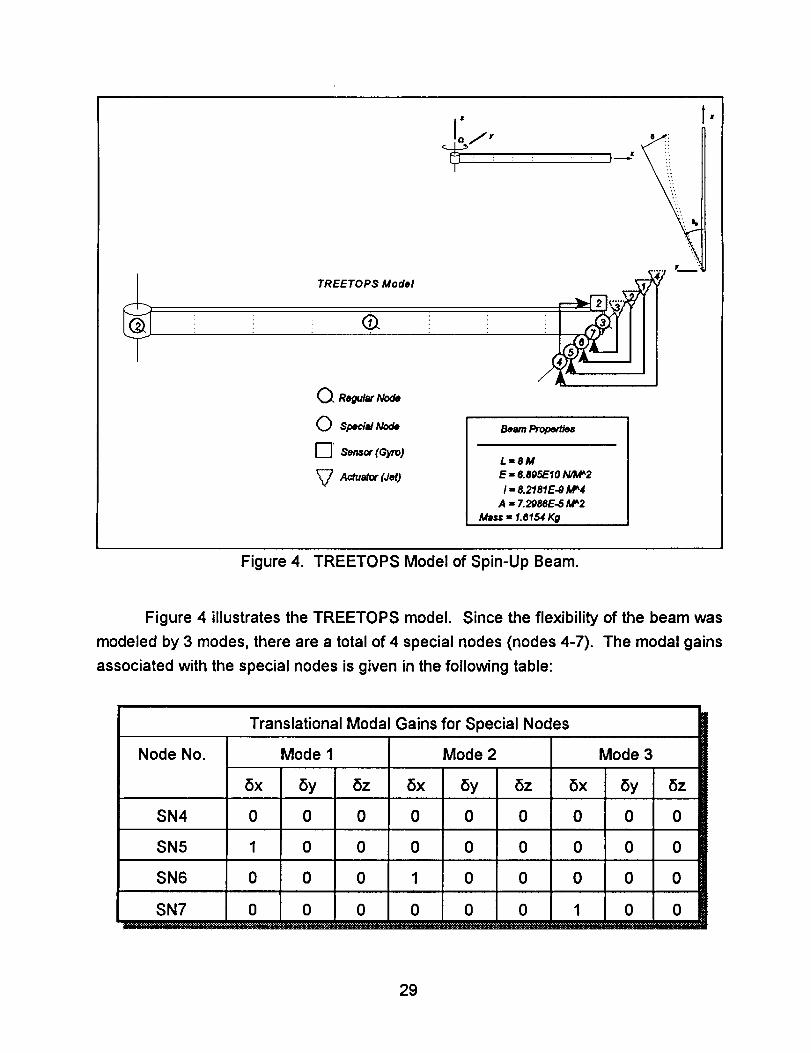
TREETOPS Model

(_ Regular Node

0 Sp_-_,/Node

[]" Sensor (Gyro)

_ Actuator (Jet)

Beam Froperti_

L=SME = 6.895E10 N/IVP2

I - 8.2181E-9 MA4A = 7.2986E-5 IVP2

= 1.6154 Kg

Figure 4. TREETOPS Model of Spin-Up Beam.

Figure 4 illustrates the TREETOPS model. Since the flexibility of the beam was

modeled by 3 modes, there are a total of 4 special nodes (nodes 4-7). The modal gains

associated with the special nodes is given in the following table:

Node No.

SN4

SN5

SN6

SN7

Translational Modal

Mode 1

6x 6y 6z

0 0 0

1 0 0

0 0 0

0 0 0

Gains for Special Nodes

Mode 2

6x 6y 6z

0 0 0

0 0 0

1 0 0

0 0 0

Mode 3

6x 6y 6z

0 0 0

0 0 0

0 0 0

1 0 0

29

All rotational modal deflections (gains) are zero for the special nodes. From the table it

can be seen that special node 4 (SN4) is capable of only sensing rigid body motions since

it has zero gains in each of the flexible modeshapes. SN5 can sense (and effect) motions

associated with mode 1 because of the unit 5x gain in this modeshape. However, SN5

cannot sense modes 2 and 3. The other special nodes have similar modal sensing and

effecting capabilities.

At this point, the reason for "designing" the modal gains associated with the special

points in the way illustrated by the previous table can now be made apparent. Since the

user controller produces the modal forces associated with the geometric stiffening terms,

the model needs to have a node (i.e., a special node) in which only the first mode is

effected by any load applied to this node. Similarly, the model should possess nodes in

which only the second (or third) mode is effected (driven) by an applied load. The reasons

that the first special node has no flexible modal gains is two-fold. First, the motion

stiffening terms need to have access to the rigid body accelerations and angular rates,

thus this special node is the ideal location to place the appropriate sensors. Secondly,

a node is required which can be used to drive only the rigid body motions of the structure.

This is necessary because a force acting on SN5 drives both mode 1 and the rigid body

modes. Since the geometric stiffening terms should not effect the rigid body motions, the

rigid body modes must be undriven. This is accomplished by simply applying the negative

of the load applied to the SN5 node to the SN4 node. Similarly, the negative of the SN6

and SN7 applied geometric stiffening loads is also applied to the SN4 node.

For the spinning beam problem, if Node 2 is considered the origin for the calculationg

of the F I vectors, then the only modal geometric stiffness matrix that is required is KoI,

which is associated with the A/(9 ) = 00z= term. The a, term is not considered is due to the

fact that the angular acceleration does not induce axial loads in the beam--hence the

geometric stiffness matrix associated with a z is zero.

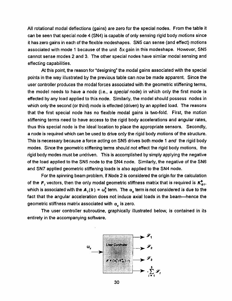
The user controller subroutine, graphically illustrated below, is contained in its

entirety in the accompanying software.

(J_z

m_=,.

!iii!iii!iii!iiiiiiiiii_iiii!iii!ii!i_i!_iiiiii!ii_iiiiiiiiiiii!iii!_iiiiiill_ 3r_

iiiiiii iii_i!iiii:ii:?:ii_il#_i!!iii!:_i!iiii!ii!i!!i! iiiii:

3

/-t

3O

As a final note, it is important that the user include all five of the modal integrals that

TREETOPS accepts in the <...>.fix file. These terms play an especially significant role

in the system response when geometric stiffening is being considered.

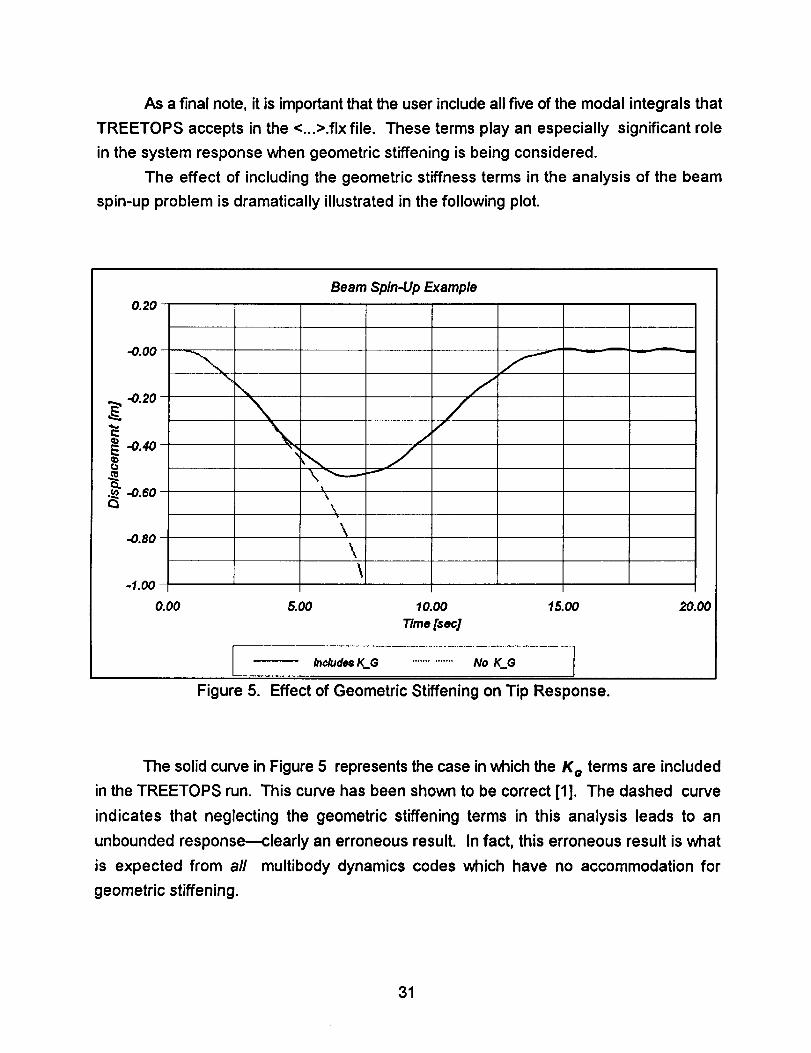
The effect of including the geometric stiffness terms in the analysis of the beam

spin-up problem is dramatically illustrated in the following plot.

Beam Spin-Up Example

0.20-

_.00 -

-0.20- :

_ -0.40-

._ -0.60-

-0.80 -

-1.00-

\\\\

v

0.00 5.00 10.00 15.00 20.00

Time [-_ec]

Include=K_G .............. No K_G

Figure 5. Effect of Geometric Stiffening on Tip Response.

The solid curve in Figure 5 represents the case in which the K o terms are included

in the TREETOPS run. This curve has been shown to be correct [1]. The dashed curve

indicates that neglecting the geometric stiffening terms in this analysis leads to an

unbounded response---clearly an erroneous result. In fact, this erroneous result is What

is expected from all multibody dynamics codes Which have no accommodation for

geometric stiffening.

31

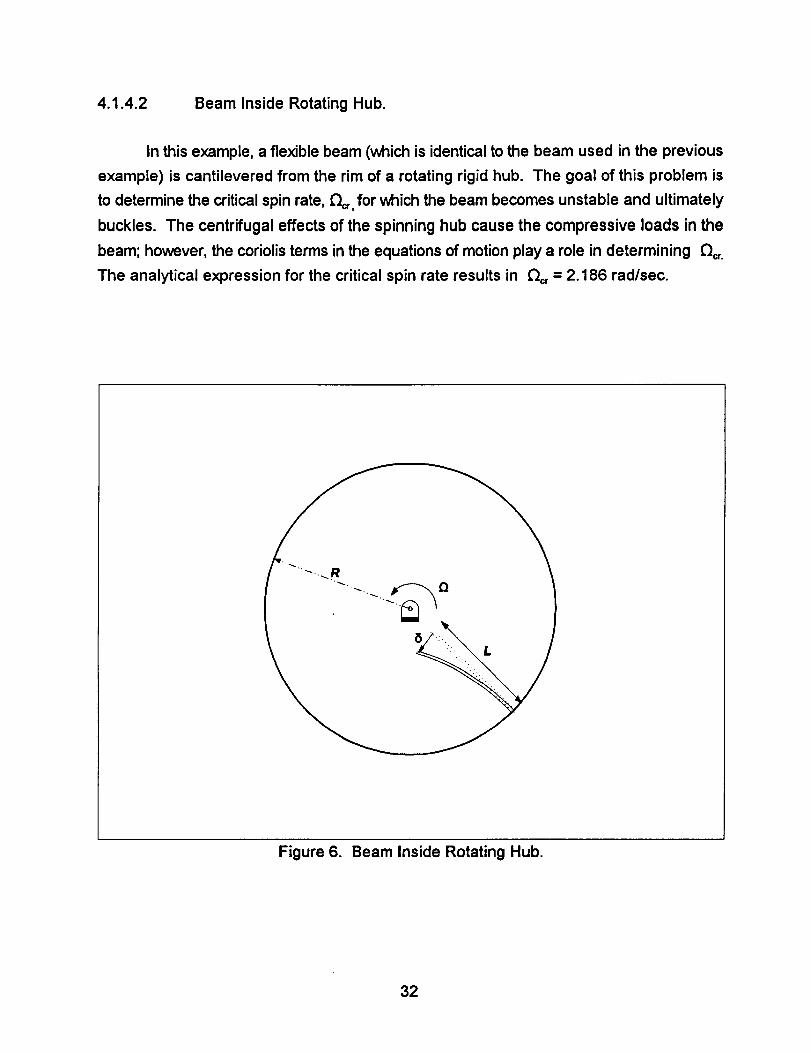
4.1.4.2 Beam Inside Rotating Hub.

In this example,a flexible beam (which is identicalto the beam used in the previous

example) is cantilevered from the rim of a rotating rigid hub. The goal of this problem is

to determine the critical spin rate, _. for which the beam becomes unstable and ultimately

buckles. The centrifugal effects of the spinning hub cause the compressive loads in the

beam; however, the coriolis terms in the equations of motion play a role in determining _°r.

The analytical expression for the critical spin rate results in _"_cr -- 2.186 rad/sec.

Figure 6. Beam Inside Rotating Hub.

32

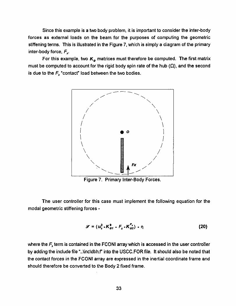
Since this example is a two body problem, it is important to consider the inter-body

forces as external loads on the beam for the purposes of computing the geometric

stiffening terms. This is illustrated in the Figure 7, which is simply a diagram of the primary

inter-body force, Fx.

For this example, two K o matrices must therefore be computed. The first matrix

must be computed to account forthe rigid body spin rate of the hub (Q), and the second

is due to the Fx =contact" load between the two bodies.

//

\

//

!

\\

\

f

• O

\\

\\\I/

//

//

Figure 7. Primary Inter-Body Forces.

The user controller for this case must implement the following equation for the

modal geometric stiffening forces -

= = J=,.fr = (OOz.K= 1 . Fx .K=2) . q (20)

where the Fx term is contained in the FCONI array which is accessed in the user controller

by adding the include file =.._inc\dbh.f"into the USCC.FOR file. It should also be noted that

the contact forces in the FCONI array are expressed in the inertial coordinate frame and

should therefore be converted to the Body 2 fixed frame.

33

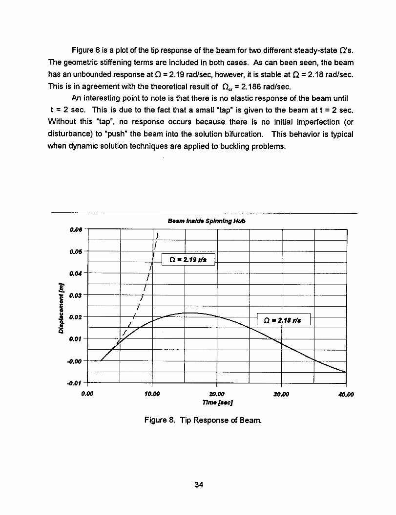
Figure 8 is a plot of the tip responseof the beam for two different steady-state Q's.

The geometric stiffening terms are included in both cases. As can been seen, the beam

has an unbounded response at Q = 2.19 rad/sec, however, it is stable at Q = 2.18 rad/sec.

This is in agreement with the theoretical result of _=r = 2.186 rad/sec.

An interesting point to note is that there is no elastic response of the beam until

t = 2 sec. This is due to the fact that a small =tap" is given to the beam at t = 2 sec.

Without this =tap', no response occurs because there is no initial imperfection (or

disturbance) to =push" the beam into the solution bifurcation. This behavior is typical

when dynamic solution techniques are applied to buckling problems.

Beam Inside Spinning Hub0.06

/

0.05

0.O4

_e 0.03

i 0.02

0.0f

-O.03

I

- /

///

Y)

/

C2: 2.19 r/=

10.00 20.00

T_me[sec]

Figure 8. Tip Response of Beam.

30.00 40.00

34

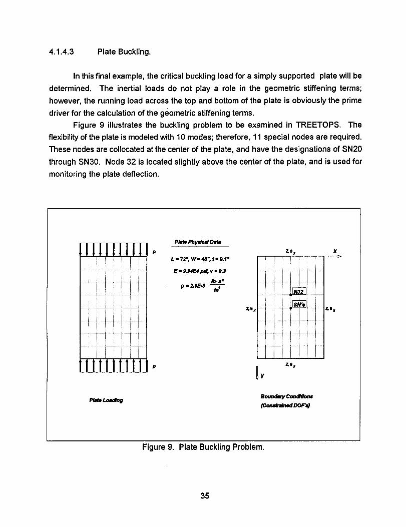
4.1.4.3 Plate Buckling.

In this final example, the critical buckling load for a simply supported plate will be

determined. The inertial loads do not play a role in the geometric stiffening terms;

however, the running load across the top and bottom of the plate is obviously the prime

driver for the calculation of the geometric stiffening terms.

Figure 9 illustrates the buckling problem to be examined in TREETOPS. The

flexibility of the plate is modeled with 10 modes; therefore, 11 special nodes are required.

These nodes are collocated at the center of the plate, and have the designations of SN20

through SN30. Node 32 is located slightly above the center of the plate, and is used for

monitoring the plate deflection.

TNTNTN-_iiiiii

...... ÷-.---.-_---.----_---.---_----..-i.-----._------._ ......

iiiii!i....... _........i.-.....÷......-_..-....._......,_.,...,.t .......

i!iiiii!iiiii!i!iiiil

.......TTTTT[T

i!iiiii!iiiill=::=I=:

...... _ @ i " @ I4 I _I f " I " II I_ " I I " " " l £ " " I " " " IiII ." III_I "I .I "I _ ......

p_ Ph_ O_

p z,e T X

L. 72. W- 44"_ t. 0.1"

E . gJ4E4 psl, v = 0_

/b.=:

p - 2.lIE-.1 /n'

,T,8 x

.......

....... ÷.......e......._.......+...-..._.....--÷_-....._ ........

......................i!i:i..

.......G..---G-.---..i..---.-G---..-I-------¢.-,----_.......

iiiiiili i iii

....... _,.,.,,.;...,...i........;....---;----..-i.-.---.i .......i_'i!!i!

.......i......._..,.....L......i.......J......_.......k.......

1,8 x

(c,=,.w_ DOt=)

Figure 9. Plate Buckling Problem.

35

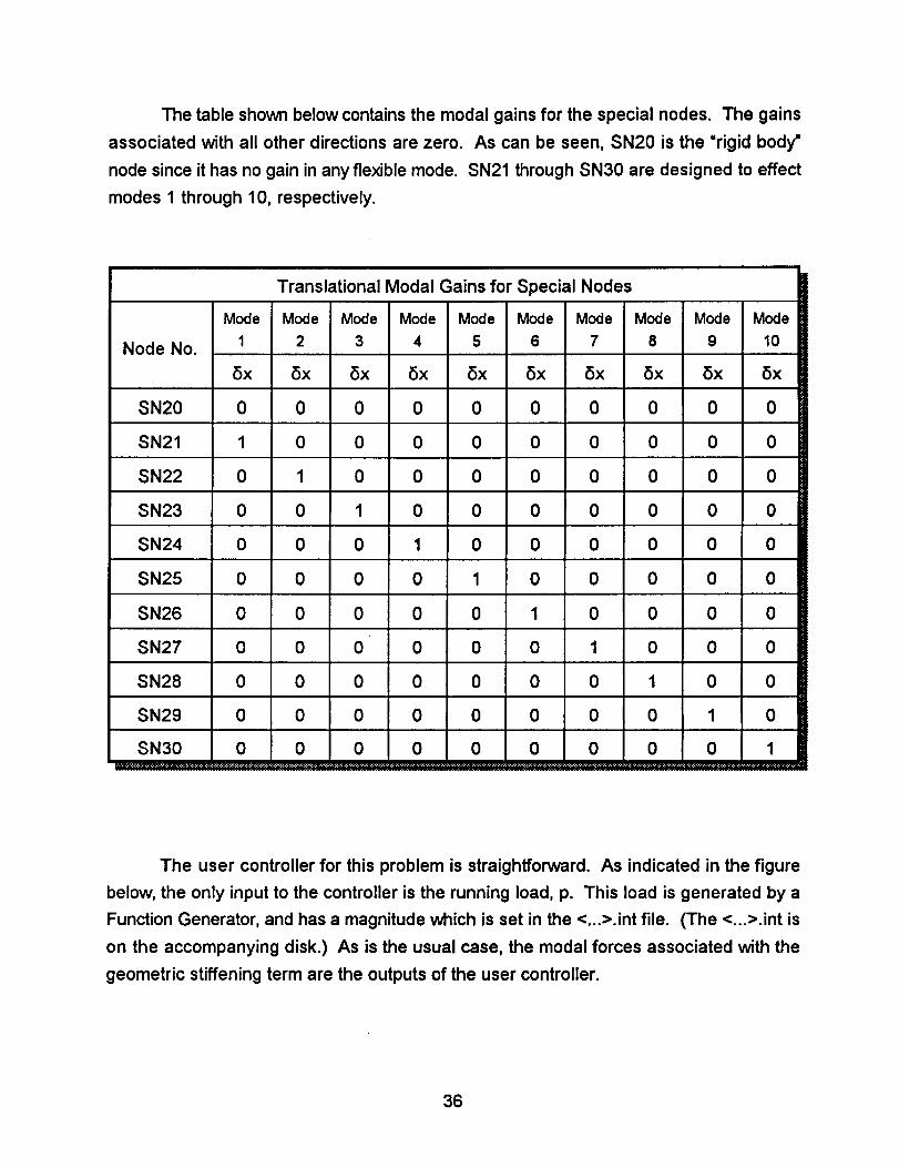
The table shown belowcontains the modal gains for the special nodes. The gains

associated with all other directions are zero. As can be seen, SN20 is the =rigid body"

node since it has no gain in any flexible mode. SN21 through SN30 are designed to effect

modes 1 through 10, respectively.

Translational Modal Gains for Special Nodes

Mode Mode Mode Mode Mode Mode Mode Mode Mode Mode

Node No. 1 2 3 4 5 6 7 8 9 10

8x 8x 8x 8x 8x 8x 8x 8x 8x 8x

SN20 0 0 0 0 0 0 0 0 0 0

SN21 1 0 0 0 0 0 0 0 0 0

SN22 0 1 0 0 0 0 0 0 0 0

SN23 0 0 1 0 0 0 0 0 0 0

SN24 0 0 0 1 0 0 0 0 0 0

SN25 0 0 0 0 1 0 0 0 0 0

SN26 0 0 0 0 0 1 0 0 0 0

SN27 0 0 0 0 0 0 1 0 0 0

SN28 0 0 0 0 0 0 0 1 0 0

SN29 0 0 0 0 0 0 0 0 1 0

SN30 0 0 0 0 0 0 0 0 0 1

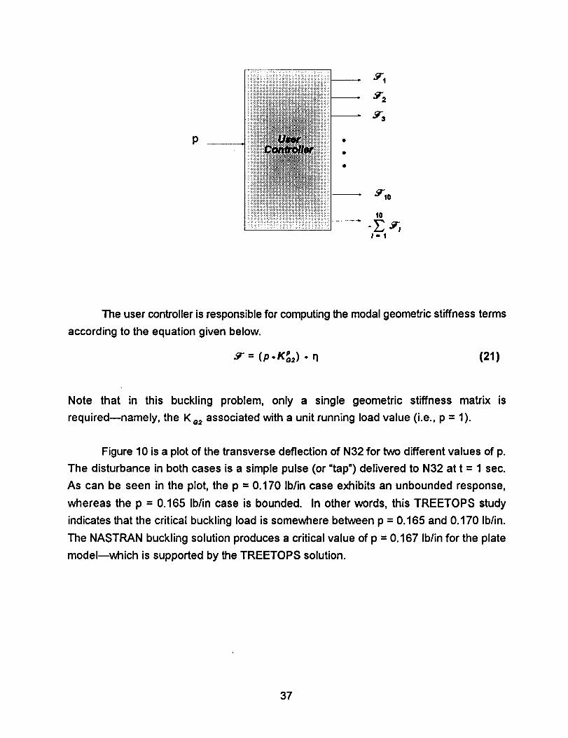
The user controller for this problem is straightforward. As indicated in the figure

below, the only input to the controller is the running load, p. This load is generated by a

Function Generator, and has a magnitude which is set in the <...>.int file. (The <...>.int is

on the accompanying disk.) As is the usual case, the modal forces associated with the

geometric stiffening term are the outputs of the user controller.

36

P

_i!!!iiiiiiiiiiii!iiiiiiii:ii!iiiiiiiiiiiiiiiiiiiiiiiiiiiiiiiiiiiiiiiiiiiiiiiiiii!iiiiiii_i_i

iil.++::++.+++::++i!::++_._+_+I++ +++++++++++++i++++: •+++++++++++_++++++++++++++++++++++++++

;iii!i::_}iii!iiii_!ii::i!!i!_!iiiiiii!!!i!_iiiiiii;!_!i!i1iii_iiiii!i_i!i:.i!i_i!i_i::i_ii_ lO

I-I

The user controller is responsible for computing the modal geometric stiffness terms

according to the equation given below.

._" = (p.K_) • q (21)

Note that in this buckling problem, only a single geometric stiffness matrix

required--namely, the K e= associated with a unit running load value (i.e., p = 1).

is

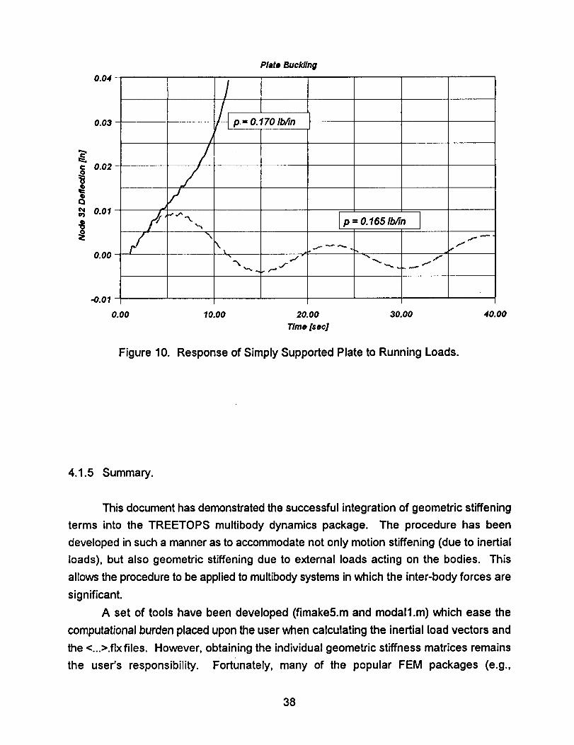
Figure 10 is a plot of the transverse deflection of N32 for two different values of p.

The disturbance in both cases is a simple pulse (or "tap') delivered to N32 at t = 1 sec.

As can be seen in the plot, the p = 0.170 Ib/in case exhibits an unbounded response,

whereas the p = 0.165 Ib/in case is bounded. In other words, this TREETOPS study

indicates that the critical buckling load is somewhere between p = 0.165 and 0.170 Ib/in.

The NASTRAN buckling solution produces a critical value of p = 0.167 Ib/in for the plate

model--which is supported by the TREETOPS solution.

37

0.04 -

0.03 -

0.02-

¢_ O.01-eq

0.00 -

-0.01 -

/\

Plate Buckling

_ p = 0.170/bAn

\\

*'_ .f

p = O.165 Ib/in

fp.

f

0.00 10.00 20.00 30.00 40.00

Time [=ec]

Figure 10. Response of Simply Supported Plate to Running Loads.

4.1.5 Summary.

This document has demonstrated the successful integration of geometric stiffening

terms into the TREETOPS multibody dynamics package. The procedure has been

developed in such a manner as to accommodate not only motion stiffening (due to inertial

loads), but also geometric stiffening due to external loads acting on the bodies. This

allows the procedure to be applied to multibody systems in which the inter-body forces are

significant.

A set of tools have been developed (fimake5.m and modall.m) which ease the

computational burden placed upon the user when calculating the inertial load vectors and

the <...>.flxfiles. However, obtaining the individual geometric stiffness matrices remains

the user's responsibility. Fortunately, many of the popular FEM packages (e.g.,

38

NASTRAN, h,NSYS, etc.) are capable of producing the required geometric stiffness

matrices.

The current methodology for computing the modal geometric stiffening terms is

carried out inside the =user controller" within TREETOPS. The inputs to the controller are

the various rigid body accelerations and angular rate values, as well as the magnitudes

of the external loads. The outputs of the controller are the modal forces associated with

the geometric stiffness terms. The modal forces are applied through a series of =jet"

actuators to a set of special nodes which possess modal gains =designed" in such a way

as to make it possible to selectively drive the individual modes of the body in question.

39

4.2 Mass Integrals for Multibody Simulations

4.2.1 Introduction

This report will present a theoretical discussion on the calculation of mass

or modal integrals common to the equations of motion of multibody systems. An

algorithm and accompanying FORTRAN program will also be described to compute

these terms from lumped Or consistent mass matrices.

4.2.2 Derivation of Mass Integrals

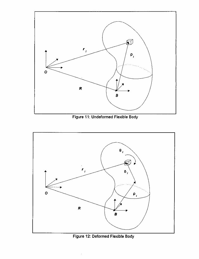
Shown in Figure 11 is an undeformed generic flexible body.

continuous body be discretized into a system of p nodal bodies, with mass

inertia I_ , and n total degrees of freedom; R

inertial frame O to the body fixed frame B; and p

Let the

m_ and

is the position vector from the

is the body fixed vector locating

the undeformed position of the nodal body I relative to B. Body deformation is

defined through degrees of freedom at the nodes. Each node may have up to six

degrees of freedom. The nodal degrees of freedom are placed in a state vector X.

40

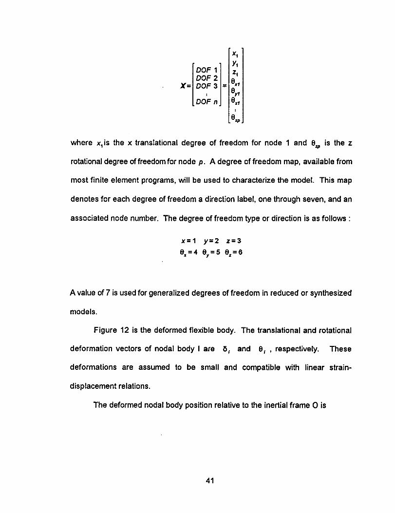
xl

roo lpY'z,I DOF 2 ex'

X= i DOF3= e_[ DOF n 8zl

t

.6z#

where x1is the x translational degree of freedom for node 1 and e_ is the z

rotational degree of freedom for node p. A degree of freedom map, available from

most finite element programs, will be used to characterize the model. This map

denotes for each degree of freedom a direction label, one through seven, and an

associated node number. The degree of freedom type or direction is as follows :

x=l y=2 z=3

e =4 e,=s e,=6

A value of 7 is used for generalized degrees of freedom in reduced or synthesized

models.

Figure 12 is the deformed flexible body.

deformation vectors of nodal body I are 8,

deformations are assumed to be small and

displacement relations.

The translational and rotational

and e_ , respectively. These

compatible with linear strain-

The deformed nodal body position relative to the inertial frame O is

41

I

0

R

B

Figure 11: Undeformed Flexible Body

0

B

Figure 12: Deformed Flexible Body

rl=R÷pl,,81

The inertial translational velocity of nodal body I is

where ¢o is the angular velocity of the bodyfixed frame B with respect to 0 and 8_

is the time rate of change of the deformation relative to B.

The kinetic energy of the system can be written as

p_

I=t 2" + +

The elastic deformations will now be described using the assumed modes

technique. In this technique, the elastic deformations of the flexible body are

approximated through a linear combination

functions and generalized time coordinates.

freedom discretized structure.

nodal body I are written as

of the products of spatial shape

The shape functions are typically a

subset of normal modes derived from a discretized or finite element model of the

component.

For this derivation, there are at most n shape functions for the n degree of

The translational and rotational deformations for

n rood==

,jrll1',t

n mo¢t_

J=l

43

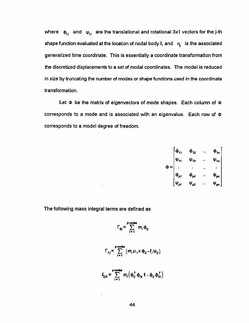
where 4)1] and qJij are the translational and rotational 3xl vectors for the j-th

shape function evaluated at the location of nodal body I, and rlj is the associated

generalized time coordinate. This is essentially a coordinate transformation from

the discretized displacements to a set of modal coordinates. The model is reduced

in size by truncating the number of modes or shape functions used in the coordinate

transformation.

Let 4) be the matrix of eigenvectors of mode shapes. Each column of ¢

corresponds to a mode and is associated with an eigenvalue. Each row of ¢

corresponds to a model degree of freedom.

_11 _12 "'" ¥1n

I I ... I

,i>,,, <l>,,,... ,l>,,,,tlJpl _p2 "-. _m

The following mass integral terms are defined as

p node=

Fill = _ rnilll uI-1

p/l_tll

Flj= I_1 (miplxiliu+lllPu)

p noel=

I,,1

T -

44

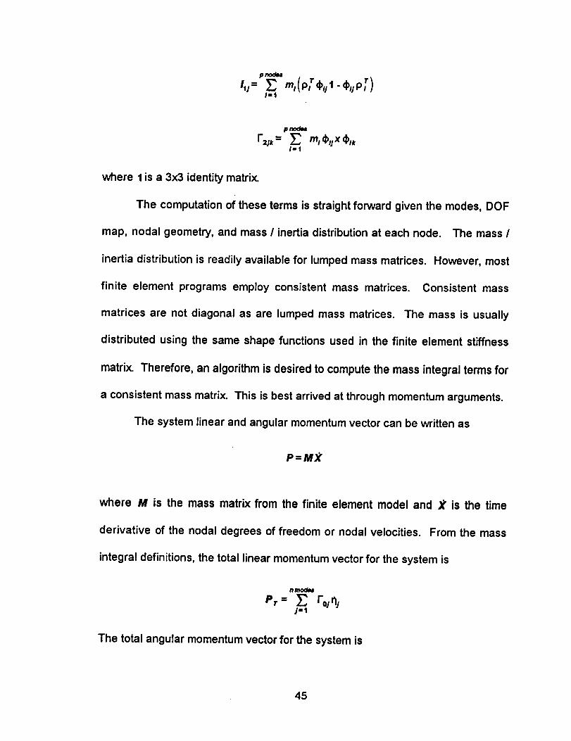
p tmde=

I,.I

pnod_

I,,t

where I is a 3x3 identity matrix.

The computation of these terms is straight forward given the modes, DOF

map, nodal geometry, and mass / inertia distribution at each node. The mass /

inertia distribution is readily available for lumped mass matrices. However, most

finite element programs employ consistent mass matrices. Consistent mass

matrices are not diagonal as are lumped mass matrices. The mass is usually

distributed using the same shape functions used in the finite element stiffness

matrix. Therefore, an algorithm is desired to compute the mass integral terms for

a consistent mass matrix. This is best arrived at through momentum arguments.

The system linear and angular momentum vector can be written as

P=M_'

where M is the mass matrix from the finite element model and X is the time

derivative of the nodal degrees of freedom or nodal velocities. From the mass

integral definitions, the total linear momentum vector for the system is

n mode=

•',r= ro1, 1J=l

The total angular momentum vector for the system is

45

Now, the system momentum vector will be expressed in terms of modal coordinates.

P= M2= MqJ q

pnod_

P_= _ P,u'P,xPrlI-t

The system momentum vector for the j'th mode is simply

I tPTq

Pj=M,jqj=[pfq

where Prq and PA_Sare the system linear and angular momentum vectors for node

I and mode j. The system momentum vector can be written as

n mo¢_

p=EpjJ. 1

The total system linear momentum vector is therefore

n modm p nodm n modm

P,.= E E EJ-t I.t J-t

Now define the product of the mass matrix and the mode shape vector as

Md)j = Aj

The system momentum vector from the j'th mode can then be expressed as

Pj=Ajq I

where

47

and

Au:IATq]LA,,s]

A v qsis the momentum vector at the i'th node from the j'th mode. The total linear

momentum vector for the system is

n moc_ p noz_

PT = __, _, ATIsrlsJ'I I't

The first mass integral for the j-th mode is therefore seen to be

pnodw

FO! = _ AT UI"1

From similar reasoning, the total angular momentum vector of the system is written

as

n modsw p nodew

PA = _, _, (PAIj'PlXPTIJ)J"l I"1

nmodW pno(_

PA= T. T. (A,I,.P,XATIj)n,J"l I=t

The total angular momentum may also be written in terms of the second mass

integral I'ls in modal coordinates as

48

n mode=

PA= r, r,sOsJ=1

The second mass integral is therefore seen to be

p nods=

I',j= i_1 (A,,.V.p, xATv )

The remaining mass integral can be expressed in terms of Aru as

p nod==

f'ajk= _" Arls x ¢'*1.1

pnode=

I=1

,,,,(p;rA_,,1-A_,_P,_)

p nod=_

rI_I(ATTIj¢Ik I -ATIj¢,; )

49

4.2.3 Software User's Guide

A FORTRAN program based on the equations presented in Section 2.0 has

been written to compute the mass integrals for discretized flexible bodies and

output the TREETOPS .FLX file. This program is composed of the following files

"massint8.for, input.for, flx_out.for, lib_flx.for, info.inc,

inpt. inc, outpt, inc. The main program is in the filemassint8, for. Itfirst

calls the subroutine input to read the data, computes the generalized or modal

matrices and mass integrals, and then call the subroutine flx out to write the

.FLX file. The subroutine input is in the file input, for and flx out is in

flx_out, for. libflx, for contains a library of matrix / vector manipulation

routines, info. inc, inpt. inc, and outpt, inc are include files used to

pass the necessary data between the various routines, info. inc contains the

parameter statements for the maximum number of modes, nodes, and degrees of

freedom.

Upon running the program ( type massint depending on the compiler used),

the user will be queried for the names of three files. The first file name is an ascii

file containing information Which describes the model size, degree of freedom map,

discretized model node numbers, number of modes, and assorted output

information. The contents of this file will be described in more detail in the next

paragraph. The second file is also an ascii file which houses the discretized or

finite element model mass, stiffness, and damping matrices. The matrices are read

in input, for as follows •

50

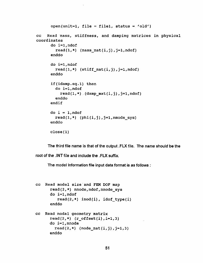
open(unit=l, file = filel, status = 'old')

cc Read mass, stiffness, and damping matrices

coordinates

do i=l,ndof

read(l,*) (mass_mat(i,j),j=l,ndof)

enddo

do i=l,ndof

read(l,*)

enddo

(stiff_mat(i,j),j=l,ndof)

if(idamp.eq.l) then

do i=l,ndof

read(l,*) (damp_mat(i,j),j=l,ndof)

enddo

endif

do i = l,ndof

read(l,*) (phi(i,j),j=l,nmode_sys)

enddo

close(l)

in physical

The third file name is that of the output .FLX file. The name should be the

root of the .INT file and include the .FLX suffix.

The model information file input data format is as follows •

cc

cc

Read model size and FEM DOF map

read(2,*) nnode,ndof,nmode_sys

do i=l,ndof

read(2,*) inod(i), idof_type(i)

enddo

Read nodal geometry matrix

read(2,*) (r offset(i),i=l,3)

do i=l,nnode

read(2,*) (node_mat(i,j),j=l,3)

enddo

51

cc

cc

cc

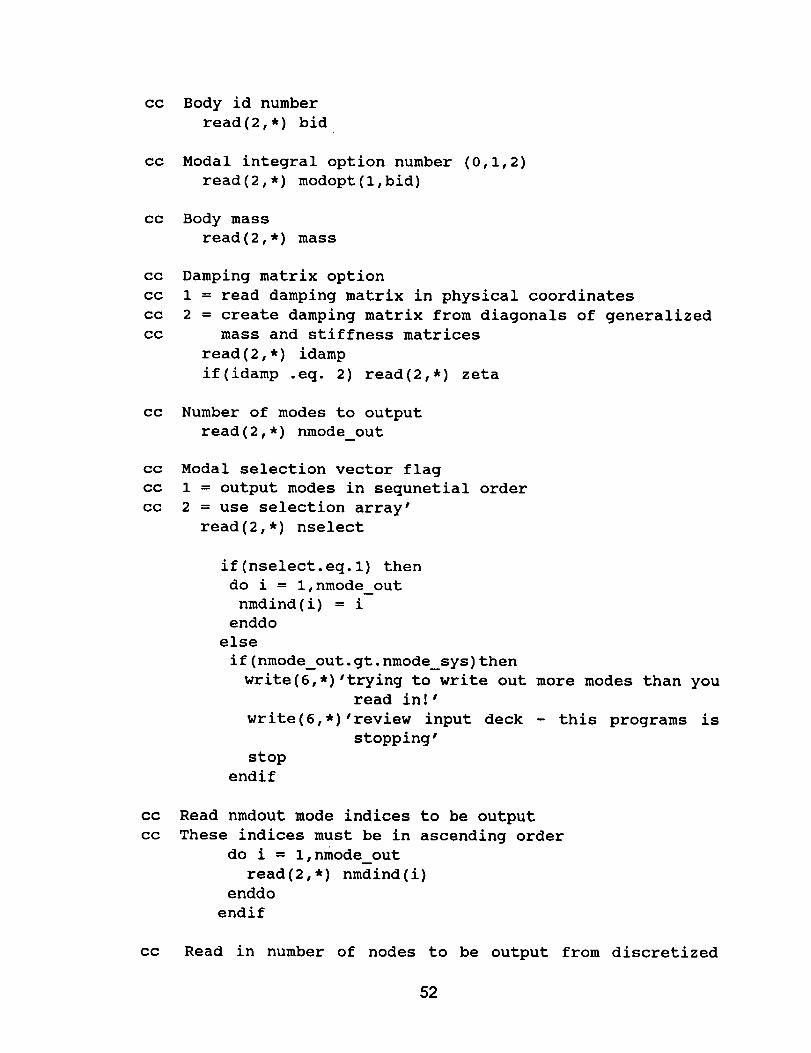
Body id number

read(2,*) bid

Modal integral option number (0,1,2)

read (2,*) modopt (l, bid)

Body mass

read(2,*) mass

cc Damping matrix option

cc 1 = read damping matrix in physical coordinates

cc 2 = create damping matrix from diagonals of generalized

cc mass and stiffness matrices

read(2,*) idamp

if(idamp .eq. 2) read(2,*) zeta

cc Number of modes to output

read(2,*) nmode out

cc Modal selection vector flag

cc 1 = output modes in sequnetial order

cc 2 = use selection array'

read(2,*) nselect

cc

cc

cc

if(nselect.eq.l) then

do i = l,nmode out

nmdind(i) = i

enddo

else

if(nmode_out.gt.nmode_sys)then

write(6,*)'trying to write out more modes than you

read in!'

write(6,*)'review input deck - this programs is

stopping'

stop

endif

Read nmdout mode indices to be output

These indices must be in ascending order

do i = l,nmode out

read(2,*) nmdind(i)

enddo

endif

Read in number of nodes to be output from discretized

52

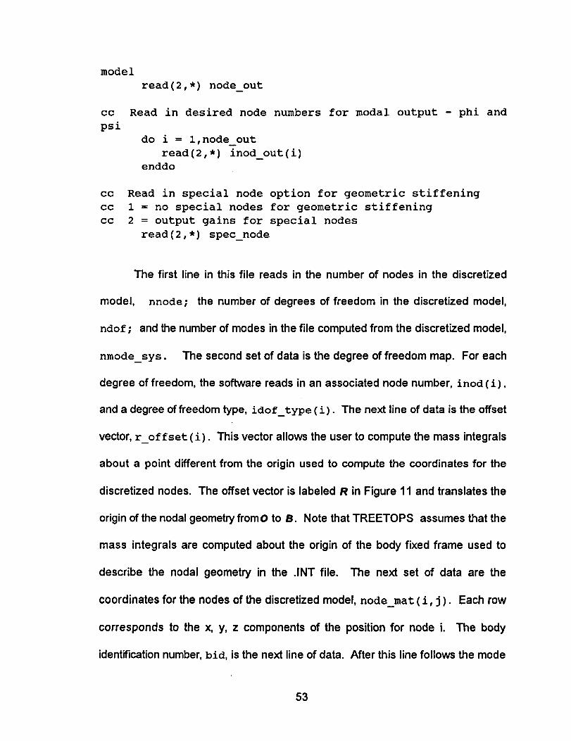
model

read(2,*) node out

CC

psi

Read in desired node numbers for

do i = l,node_out

read(2,*) inod out(i)

enddo

modal output - phi

cc Read in special node option for geometric stiffening

cc 1 = no special nodes for geometric stiffening

cc 2 = output gains for special nodes

read(2,*) spec_node

and

mode{,

ndof;

The first line in this file reads in the number of nodes in the discretized

nnode; the number of degrees of freedom in the discretized model,

and the number of modes in the file computed from the discretized model,

nmode_sys. The second set of data is the degree of freedom map. For each

degree of freedom, the software reads in an associated node number, inod (i),

and a degree of freedom type, idof_type (i). The next line of data is the offset

vector, r_offset (i). This vector allows the user to compute the mass integrals

about a point different from the origin used to compute the coordinates for the

discretized nodes. The offset vector is labeled R in Figure 11 and translates the

origin of the nodal geometry fromO to S. Note that TREETOPS assumes that the

mass integrals are computed about the origin of the body fixed frame used to

describe the nodal geometry in the .INT file. The next set of data are the

coordinates for the nodes of the discretized model, node_mat (i, j ). Each row

corresponds to the x, y, z components of the position for node i. The body

identification number, bid, is the next line of data. After this line follows the mode

53

option number (0,1,2), modopt (1, bid). A value of 0 will direct the software to

compute all mass integrals; a value of 1 will compute only the zero and first order

terms; and a value of 2 will output only the zero order modal integrals. The body

mass, mass, is input next to scale the alpha modal integrals. Following the mass

is the damping matrix option flag idamp. A value of 1 directs the code to read in

a physical damping matrix after the stiffness matrix. A value of 2 will enable the

code to compute a diagonal generalized damping matrix from the product of twice

the input value of zeta and the square root of the ratio of the generalized stiffness

matrix diagonal and the generalized mass matrix diagonal. The next line of data is

the value of zeta, zeta, if the value of idamp is 2. Otherwise, the next line is the

number of modes to be output in the .FLX file, nmode out. The user may select

which modes to output through the modal selection vector. A value of 1 for

nselect will direct the code to output the first nmode out modes in the data file.

A value of 2 will direct the code to read in the selection array nmdind (i)as an

array of ascending output mode numbers, one per line. The next line of data is the

number of discretized model nodes to be output, node_out. After this is the array

of desired output node numbers, inod_out, in ascending order and one per line.

Finally, the last line of data in the special nodes flag, spec_node, for use in

incorporating geometric stiffness matrices into the model. A value of 1 for this flag

will cause the code to output no special nodes. A value of 2 will direct the software

to write out nmode + I special nodes. The first special node is the rigid body node

and will have zero modal gains. The remaining special nodes are given a modal

gain of I for x translation for one mode each. The special nodes are appended to

54

the end of the normal nodes in the .INT file.

The user of this code may readily modify input, for for specific data

bases. A set of example data files is supplied with this software to test it upon

installation to a particular computer system. The model information file name is

test. inp. The discretized data file name is test. mat. The output .FLX file is

test. flx and matches the data computed using modall .m in MATLAB.

55

5.0 Conclusions

This report has described the enhancements and additions to the

TREETOPS suite of dynamic analysis tools by Oakwood College. The Software

DesignDocument, inclusionof geometric stiffness into TREETOPS, as well as the

development of user-friendly modal integral tools have been presented.

The SoftwareDesignDocumentprovides a description of the argument lists

and internal variables used in each subroutine of the TREETOPS suite.

Geometrically nonlinear response problems can be addressed by incorporating a

specially designed =User Controller" into the suite. Both Fortran and MATLAB

forms of user-friendly modal integral tools were delivered under the provisions of

contract NAS8-40194.

Additionally, a new set of User and Theory Manuals were prepared under

this contract. These items, along with the others listed, should provide the

inexperienced user more confidence in the use of the TREETOPS package. The

Software Design Document is intended to allow the advanced user a more rapid

and complete immersion into the code. This will no doubt ease the burden of future

analysts who attempt to provide further enhancements to the TREETOPS suite of

codes.

56

References

[1] Honeywell, =Users Manual for CONTOPS VAX Application," Clearwater,Florida, January, 1987

[2] Honeywell, "Software Design Document," Clearwater, Florida, 1985

[3] Dynacs Engineering Co., "TREETOPS Software Verification Manual,"Florida, 1988

[4] Honeywell, "Users Manual for TREETOPS," Clearwater, Florida, June, 1984

[5] Dynacs Engineering Co., =TREETOPS Theory Manual," Florida, November29, 1990

[6] Dynacs Engineering Co., =Geometric Nonlinearity in TREETOPS," NAS8-

38092, Report Number : r 30-30, December 16, 1991

[7] Howsman, T. G., =Dynamic Analysis of a Class of Geometrically Nonlinear

Multibody Systems," Ph.D. Dissertation, University of Alabama in Huntsville,1993

57

List of Acronyms

NASTRAN

DOS

MSC

COTR

FEM

DMAP

National Aeronautics and Space Administration Structural Analysis

Disk Operating System

MacneaI-Schwendler Corporation

Contracting Officer's Technical Representative

Finite Element Model

Direct Matrix Alter Program

58

Form Approved

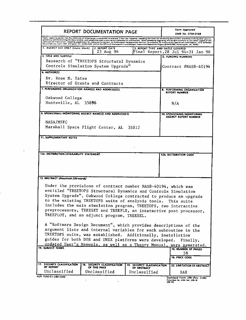
REPORT DOCUMENTATION PAGE OMa_o o704_,8a

P,d_.¢ t_Dor_l_ t_rd_n _ t_,_ (ol_'_Jo_ of w_formBIiOn rt ('stlm.ted 10 .ref=<_. ! hour D_¢ ti_Oe,,_, iflCltd,ng Ih,ip brae Io r *.ev,_*e*r,g ge.tirvctDont. _,e=r¢h,_q _._t,_,g d=tJ to_rce%

q=t_*_ncj h_d _a,n_J,_n 9 Ih_ d=t_ _. _td (e*_esmq a_,d ,_-v,_..m<j |h_ coal.,on of mfo*m=z*on ¢._r.d comm_rntl rd,_ 9 th,t t_urd_ e=sl,m_le ¢_ =n v 01_ .t_-¢_ of t_n(ots_t,o_ of ,_ c.m=¢_on ,r,_lt_/,_ _t,or_ fo* e_dwJ_ th,_ t_rd_n to wmsh,_glC_ N_u,rler_ $e_,¢_'% t_r_<1o_l_ I_fO_mlt,on Ope_t,oe_ _ Re_OnLS. 1715 Jeffe_,on

O_.t _,qhwe_. $_t_ 1204 Arl,_tO_ VA _2 _1_*-1302. _nd to Ct_ Off,ce of kt_n_.w_enl _r_d Bud9_l , Par_ort. R_dtKl_em Pf© eel (0_0al-0 t_l_). Wa.,_*r_ton. O( _0_1].

1. AGENCY USE ONLY (Leave blank) 2. REPORt" DATE 3. REPORT TYPE AND DATES COVERED

23 Aug 96 Final Report,28 Jul 94-31 Jan 964 .;L_ ANDSUaTI;_E s FUND,N_NUMaERS

Research of "TREETOPS Structural Dynamics

Controls Simulation System Upgrade"

6. AUTHOR(S)

Dr. Rose M. Yates

Director of Grants and Contracts

7. PE_ORMING ORGAN_ATION NAME(S) AND ADDRESSES)

Oakwood College

Huntsville, AL 35896

9--_)ONSOmNG/MON_OmNGAGEN_ NAME{S) ANDADDRES$(E$)

NASA/MSFC

Marshall Space Flight Center, AL 35812

!l._P'PtJEMENTARYNO,E$

Contract #NAS8-40194

8. PERFORMING ORGANIZATIONREPORT NUMBER

N/A

10. SPON SORJNG I MONITORINGAGENCY REPORT NUMBER

12a. DISTRIBUTION/AVAILABILITY STATEMENT

13. ABSTRACT (Max*mum 200 words)

12b. OISTPJBUTION CODE

Under the provisions of contract number NAS8-40194, which was

entitled "TREETOPS Structural Dynamics and Controls Simulation

System Upgrade", Oakwood College contracted to produce an upgrade

to the existing TREETOPS suite of analysis tools. This suite

includes the main simulation program, TREETOPS, two interactive

preprocessors, TREESET and TREEFLX, an interactive post processor,

TREEPLOT, and an adjunct program, TREESEL.

A "Software Design Document", which provides descriptions of the

argument lists and internal variables for each subroutine in the

TREETOPS suite, was established. Additionally, installation

guides for both DOS and UNIX platforms were developed. Finally,

updated User's Manuals_ as wel ! as a Theory Manual_ were generated.14._ECT TERMS 1S.NUMBEROFPAGES

17. SECU_/TYCLASSIFICATION. 18. SECURITYCLASSIFICATIONOFREPORT O_T'IS PA_EUnclassified Unclassified

tg. SECURITY CLASSIFICATIONOF ABSTRACT

Unclassified

NSN 7540--01-280-5500

58I£. PRICE CODE

20. LIMITATION OF ABSTRACT

SAR

Standard Form 29B (Rev. _-8g)_e_7,bed by _5_ 51d ZJ_8