Nano-mechanics for Intelligent Materials (1/2)
43
Nano-mechanics for Intelligent Materials (1/2) Giorgio MATTEI
Transcript of Nano-mechanics for Intelligent Materials (1/2)

Nano-mechanics for Intelligent Materials (1/2)
Giorgio MATTEI

From sample mechanical behaviour to properties
Sample
Mechanical
behaviour
Testing type and method
𝜎
𝜀
ሶ𝜀
𝑡
𝜎 𝑓
DMA output
ሶ𝜀𝑀 output
Measured mechanical
behaviour (raw data)
...
𝐸𝑎𝑝𝑝
ሶ𝜀
𝑓
𝐸′
𝐸′′
𝐸
Apparent modulus
Storage & Loss moduli
Mechanical properties
...
𝑡
𝜀
ሶ𝜀
Bulk
Indentation
Frequency
(DMA)
Strain rate ( ሶ𝜀𝑀)
... ...
𝑡
𝜀 𝑓
Type Method
Analysis
model

Material mechanical properties
• Little consensus in the literature
S Marchesseau et al, Progr in Biophys and Mol Biol 103:185-96 (2010) G Mattei and A Ahluwalia, Acta Biom 45:60-71 (2016)

Elastic, viscous and visco-elastic response
Deborah Number
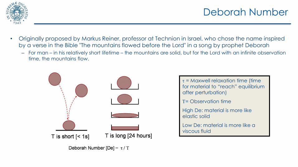
• Originally proposed by Markus Reiner, professor at Technion in Israel, who chose the name inspired by a verse in the Bible "The mountains flowed before the Lord" in a song by prophet Deborah
– For man – in his relatively short lifetime – the mountains are solid, but for the Lord with an infinite observation
time, the mountains flow.
= Maxwell relaxation time (time
for material to “reach” equilibrium
after perturbation)
= Observation time
High De: material is more like
elastic solid
Low De: material is more like a
viscous fluid

Examples of viscoelastic materials

Stress Relaxation
When a body is deformed (or strained) and that deformation (or strain) is held constant,
stresses in the body reduce with time.
Figure from Fung “Biomechanics” 2nd ed.

Creep
When a body is loaded (or stressed) and the stress is held constant, the body continues to
deform (or strain) with time.
Figure from Fung “Biomechanics” 2nd ed.

Hysteresis
When a body subjected to cyclic loading, load-displacement (or stress-strain) behavior for increasing
loads is different than behavior for decreasing loads.
The area between the curves represents energy loss (dissipation).
Figure from Fung “Biomechanics” 2nd ed.
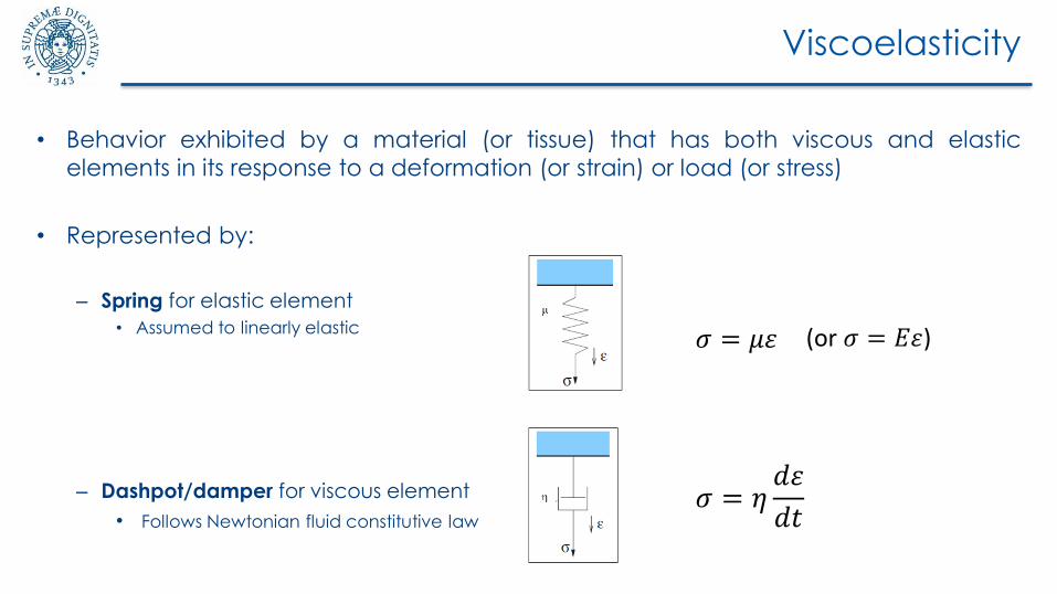
Viscoelasticity
• Behavior exhibited by a material (or tissue) that has both viscous and elastic
elements in its response to a deformation (or strain) or load (or stress)
• Represented by:
– Spring for elastic element
• Assumed to linearly elastic
– Dashpot/damper for viscous element
• Follows Newtonian fluid constitutive law 𝜎 = 𝜂
𝑑𝜀
𝑑𝑡
𝜎 = 𝜇𝜀 (or 𝜎 = 𝐸𝜀)

Lumped parameter models
The Maxwell, Voigt and Kelvin (SLS)
models are all composed of
combinations of linear springs (µ or E)
and dashpots (η).
A linear spring with spring constant
theoretically produces a deformation
proportional to the load.
A linear dashpot with coefficient of
viscosity produces a velocity
proportional to the load.

Maxwell model
• Represented by a purely viscous damper (η) and a purely elastic spring (E) connected in series
• The model can be represented by the following differential equation (DEQ):
• Predicts/models a stress that decays exponentially with time to zero with permanentdeformation
• Model doesn’t accurately predict creep (constant stress). Predicts that strain will increaselinearly with time. Actually strain rate decreases with time
Stress relaxation experiment
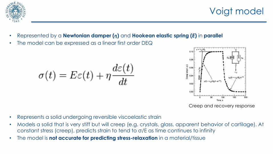
Voigt model
• Represented by a Newtonian damper (η) and Hookean elastic spring (E) in parallel
• The model can be expressed as a linear first order DEQ
• Represents a solid undergoing reversible viscoelastic strain
• Models a solid that is very stiff but will creep (e.g. crystals, glass, apparent behavior of cartilage). Atconstant stress (creep), predicts strain to tend to σ/E as time continues to infinity
• The model is not accurate for predicting stress-relaxation in a material/tissue
Creep and recovery response

Standard Linear Solid (SLS) model
• Represented by a Hookean spring in parallel to a Newtonian damper + Hookean spring arm
• The model can be expressed as a linear first order DEQ:
• Represents a solid undergoing an elastic and a reversible viscoelastic strain
• At constant stress (creep), predicts an initial strain from the spring which will creep over time until the parallel spring carries all the applied load
• The model is a linear approximation of viscoelastic materials/tissues that are time dependent but completely recover from applied loads
010 1
1 1
1
+ = + +
Creep and recovery response

Summary: creep and relaxation responses
xx

Generalized Models
• Generalized Maxwell model consists of Maxwell elements in parallel to a pure spring
• Generalized Voigt model consists of Voigt elements in series to a pure spring

Maxwell model creep

Creep functions
• Solving the DEQs for the Maxwell, Voigt, and Kelvin models for displacement ε = c(t), when thestress (t) is a unit step function 1(t)
• We obtain a set of results known as the creep functions
• These functions represent the elongation (strain) in the viscoelastic material which is produced by asudden application of unit stress at time = 0
c(t) = (1/ + t/)1(t) Maxwell
c(t) = 1/ (1-e-(/)t)1(t) Voigt
c(t) = 1/ER [ 1 – (1-/)e-t/]1(t) SLS
where = 1/1 , = (1/0)(1 + 0/1), and ER = 0

Maxwell model relaxation

Relaxation Functions
• Solving the DEQs for stress [(t) = k(t)] when the applied strain is a unit step function ε(t) =1(t) yields the relaxation functions
• These represent the resisting stress as a function of time
k(t) = e-(/)t1(t) Maxwell
k(t) = (t) + 1(t) Voigt
k(t) = ER [ 1 – (1 - /)e-t/]1(t) SLS
where = 1/1 , = (1/0)(1 + 0/1), and ER = 0
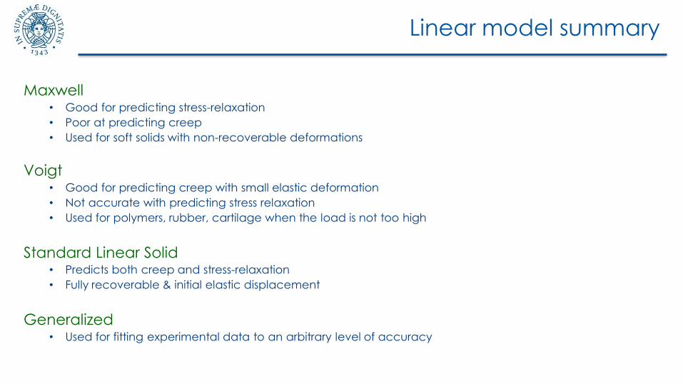
Linear model summary
Maxwell• Good for predicting stress-relaxation
• Poor at predicting creep
• Used for soft solids with non-recoverable deformations
Voigt• Good for predicting creep with small elastic deformation
• Not accurate with predicting stress relaxation
• Used for polymers, rubber, cartilage when the load is not too high
Standard Linear Solid• Predicts both creep and stress-relaxation
• Fully recoverable & initial elastic displacement
Generalized• Used for fitting experimental data to an arbitrary level of accuracy

Nano-indentation
• A popular technique to characterise material mechanical properties at the micro-scale
• Typically, a probe is brought in contact with a surface, pushed into the material and then retracted,recording load (P) and displacement (h) over time (t)
• The P-h-t data are then analysed with a range of models, such as elastic, elastoplastic, viscoelasticor poroviscoelastic, to derive material mechanical properties

Why nanoindentation?
• Ideal for probing local gradients and heterogeneities (typical of e.g. natural materials) andinvestigating their hierarchical multi-scale organization
• Does not require extensive sample preparation prior to testing (in contrast with most classicaltechniques, e.g. tensile testing which requires “dog-bone” shaped samples)
• Allows the measurement of very small forces and displacements (generally in the range of µN ÷ mNand nm ÷ µm, respectively)
• Requires small volumes of materials, and is thus particularly suitable for valuable samples
• Very small forces are applied, thus the technique is well suited for soft biomaterials (e.g. hydrogels),which due to their pliable and highly hydrated nature, are a challenge to characterise usingmacro-scale techniques

Why nanoindentation?
• A variety of deformation modes can be studied at typical cell length-scales by changingexperimental time scales, indenter tip geometry and loading conditions
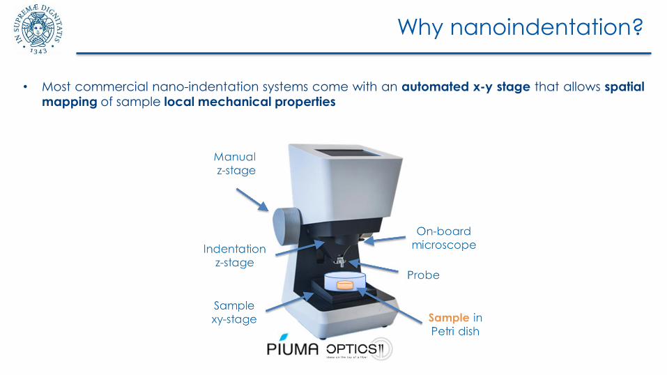
Why nanoindentation?
• Most commercial nano-indentation systems come with an automated x-y stage that allows spatialmapping of sample local mechanical properties

Why nanoindentation?
• The mechanical behavior of biological tissues generally changes with
• Thus, nanoindentation can also be attractive in the biomedical context as a potential diagnostic tool or for engineering smart cell culture scaffold based on intelligent materials
development ageing disease

ELASTIC PROPERTIES

Elastic properties: unloading curve analysis
Oliver-Pharr model
• Introduced in 1992 and revised in 2004, it is based on an elastic–plastic contact model and uses three key parameters from the indentation test:
– the peak indenter force (𝑃𝑚𝑎𝑥)
– the peak indenter displacement (ℎ𝑚𝑎𝑥)
– the unloading slope or stiffness (𝑆 = 𝜕𝑃/𝜕ℎ)

Elastic properties: unloading curve analysis
Oliver-Pharr model
• The Oliver–Pharr method begins by fitting the unloading portion of the indentation load–depthdata to the power-law relation shown below:
• Once the three fitting parameters α, m and hf are obtained, the contact stiffness S, which isdefined as the slope of the unloading curve at the maximum indentation depth, can be computedfrom
• The contact depth of the spherical indentation hc can be calculated by following the Oliver–Pharrmethod as

Elastic properties: unloading curve analysis
Oliver-Pharr model
• The contact area Ac can be computed directly from the contact depth hc and the radius of theindenter tip R
• The contact stiffness S and the contact area Ac are then used to calculate the reduced (oreffective) modulus
where β is a dimensionless correction factor which accounts for the deviation in stiffness due to thelack of axisymmetry of the indenter tip, with β=1.0 for axisymmetric indenters, β=1.012 for a square-based Vickers indenter, and β=1.034 for a triangular Berkovich punch
• β = 1 for spherical indenter tips

Elastic properties: unloading curve analysis
Oliver-Pharr model
• After obtaining the reduced modulus Er, the indentation modulus from the Oliver–Pharr methodcan be finally determined by
where vs is Poisson's ratio of the specimen, Ei and vi are respectively the elastic modulus andPoisson's ratio of the indenter. For ordinary single phase materials, the indentation modulusobtained is the elastic modulus of the specimen.
• If the indenter elastic modulus Ei is much larger than that of the specimen (e.g., SMAs, hydrogels,soft (bio)materials), the indenter can be treated as a rigid body and Eop can be simplified as

Elastic properties: loading curve analysis
Hertz model
• The analysis of the loading portion of nano-indentation data collected with a spherical tip is generally based on the Hertz model, assuming a linear elastic and isotropic material response.
• The load 𝑃 is expressed as:
where 𝑹 is the radius of the spherical indenter tip, 𝒉 is the penetration depth and 𝑬𝒆𝒇𝒇 denotes the
effective composite elastic modulus of the indenter and specimen system given by:
𝐸′ and 𝜐′ respectively refer to the modulus and Poisson’s ratio of the indenter, while the other terms refer to those of the sample
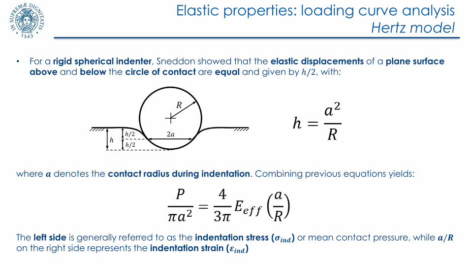
Elastic properties: loading curve analysis
Hertz model
• For a rigid spherical indenter, Sneddon showed that the elastic displacements of a plane surface above and below the circle of contact are equal and given by ℎ/2, with:
where 𝒂 denotes the contact radius during indentation. Combining previous equations yields:
The left side is generally referred to as the indentation stress (𝝈𝒊𝒏𝒅) or mean contact pressure, while 𝒂/𝑹on the right side represents the indentation strain (𝜺𝒊𝒏𝒅)
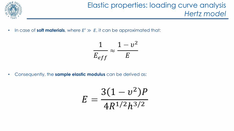
Elastic properties: loading curve analysis
Hertz model
• In case of soft materials, where 𝐸′ ≫ 𝐸, it can be approximated that:
• Consequently, the sample elastic modulus can be derived as:

Loading analysis issue: initial contact point
Ideal tests should start out of sample contact need of displacement-controlled experiments and post-measurement identification of the initial contact point
Commercial load-
controlled nano-
indenters
Load-based contact
point determination
Even small trigger load can cause
a significant pre-stress on soft samples
Cao Y et al., J Mater Res 20 (2011)
Kaufman et al.,
J Mater Res 23 (2008)

Loading analysis issue: initial contact point
• A possible solution…
Tirella A et al., JBMR A 102 (2014) Mattei G et al., J Biomech 47 (2014) Mattei G et al., JMBBM (2015)
Last point at which the
load crosses the P-h abscissa during loading
𝑷
𝒉
Unique identification of the contact point both when
✓ Snap into contact is poorly
evident
✓ Noise around zero load is present

Advantages of loading curve analysis
• Mechanical properties representative of those of the virgin material, returning a constant modulus value regardless of the maximum load (or displacement) chosen for the measurements.

Advantages of loading curve analysis
• Moreover, during unloading it is assumed that only the elastic displacements are recovered, thus methods based on the unloading curve are unsuitable for testing viscoelastic materials.
𝑺 < 0 !!!

VISCO-ELASTIC PROPERTIES

Creep
• A creep test is based on applying a constant load and measuring the change in displacementover time due to viscoelastic phenomena
• Hertz-type viscoelastic theory can be used to obtain the effective creep compliance of a materialunder a step load (𝑃0, constant over time) imposed by a spherical indenter, obtaining:
In case of soft materials where 𝐸′ ≫ 𝐸, the creepcompliance becomes:

Stress-relaxation
• Stress-relaxation can be considered the dual of creep test. It consists of measuring the loadrelaxation over time in response to a constant step indentation input (ℎ0). Assuming 𝐸′ ≫ 𝐸, therelaxation modulus can be expressed as:
Notably, in general 𝐸(𝑡) ≠ 1/𝐽(𝑡),except for 𝑡 = 0 where 𝐸 0 = 1/𝐽(0).

Useful references
• G. Mattei, G. Gruca, N. Rijnveld, A. Ahluwalia, The nano-epsilon dot method for strain rate viscoelastic
characterisation of soft biomaterials by spherical nano-indentation, J. Mech. Behav. Biomed. Mater. 50 (2015)
150–159. doi:10.1016/j.jmbbm.2015.06.015.
• M.L. Oyen, Nanoindentation of biological and biomimetic materials, Exp. Tech. 37 (2013) 73–87.
doi:10.1111/j.1747-1567.2011.00716.x.
• G. Mattei, A. Ahluwalia, Sample, testing and analysis variables affecting liver mechanical properties: A review,
Acta Biomater. 45 (2016) 60–71. doi:10.1016/j.actbio.2016.08.055.
• D. Roylance, Engineering viscoelasticity, Dep. Mater. Sci. Eng. Inst. Technol. Cambridge MA. 2139 (2001) 1–37.
• G. Mattei, L. Cacopardo, A. Ahluwalia, Micro-Mechanical Viscoelastic Properties of Crosslinked Hydrogels Using
the Nano-Epsilon Dot Method, Materials (Basel). 10 (2017) 889. doi:10.3390/ma10080889.
• H. van Hoorn, N.A. Kurniawan, G.H. Koenderink, D. Iannuzzi, Local dynamic mechanical analysis for
heterogeneous soft matter using ferrule-top indentation, Soft Matter. 12 (2016) 3066–3073.
doi:10.1039/C6SM00300A.
• M.L. Oyen, R.F. Cook, A practical guide for analysis of nanoindentation data, J. Mech. Behav. Biomed. Mater. 2
(2009) 396–407. doi:10.1016/j.jmbbm.2008.10.002.
• G. Mattei, A. Tirella, G. Gallone, A. Ahluwalia, Viscoelastic characterisation of pig liver in unconfined
compression, J. Biomech. 47 (2014) 2641–2646. doi:10.1016/j.jbiomech.2014.05.017.

Contacts
Giorgio MATTEI
Assistant Professor in Bioengineering
University of Pisa
Dept. of Information Engineering
Largo Lucio Lazzarino 1
56122 Pisa – Italy
Phone: +39 050 2218239
Mail: [email protected]