Name Your Own Price at Priceline.com:

Strategic Bidding and Lockout Periods

Chia-Hui Chen�

Academia Sinica

First version received May 2009; �nal version accepted October 2011

Abstract

A buyer suggests prices to N sellers in a time period and buys from the

seller who accepts the bid �rst. The number of bidding rounds is determined

by how frequently the buyer can make an o¤er. We show that with no limit

on the frequency and without discounting, the price path is either kept �at

initially with large jumps at the end or increasing steadily over time. Which

class of path occurs in equilibrium depends on the buyer�s trade-o¤ between

committing to a price ceiling versus �nely screening the sellers� costs. With

discounting, limiting the number of rounds mitigates the delay caused by the

reluctance to raise bids in the �rst class of equilibrium, and therefore can bene�t

the buyer. This result suggests why, in reality, bargaining parties often take

measures to make their o¤ers rigid and consequently force themselves to make

fewer o¤ers.�This paper is a revision of the �rst chapter of my dissertation submitted to MIT in 2009.

I am indebted to Glenn Ellison, Bengt Holmstrom, and David McAdams for their support andvaluable discussions. I am deeply grateful to the editor and the referees for detailed and helpfulcomments that have greatly improved this paper. I would also like to thank Junichiro Ishida, Kong-Pin Chen, Parag Pathak, Muhamet Yildiz, Sergei Izmalkov, Cyrus Chu, Chyi-Mei Chen, Ying-JuChen, Filippo Balestrieri, and participants at the MIT theory lunch seminars in 2007 and 2008,the 2009 International Conference on Game Theory, and seminars at Academia Sinica, NationalTaiwan University, and Osaka University for many suggestions and comments. Financial supportfrom my joint-a¢ liation in Academia Sinica, Research Center for Humanities and Social Sciences,is gratefully acknowledged. All remaining errors are my own.

1

1 Introduction

Priceline.com, known for its Name Your Own Price (NYOP) system, is a website

devoted to helping travelers to obtain discount rates for travel-related items such

as airline tickets and hotel stays. The NYOP mechanism works as follows. First, a

customer enters a bid that speci�es the general characteristics of the desired item

(travel dates, location, hotel rating, etc.) and the price that he is willing to pay.

Next, Priceline.com either communicates the customer�s bid to participating sellers

or accesses their private database to determine whether Priceline.com can satisfy

the customer�s speci�ed terms and the bid price. If a seller accepts the bid, the o¤er

cannot be cancelled. If no seller accepts the bid, the customer can rebid either by

changing the desired speci�cations or by waiting for a minimum period of time, the

lockout period, before submitting a new, higher price o¤er.1

To represent the Priceline auction, we use a dynamic model in which a single

buyer suggests prices to N potential sellers for a �nite number of rounds. The

number of rounds T determines the length of the lockout period. By letting T go

to in�nity, we can consider the case of no lockout period. For simplicity, we assume

that the buyer�s valuation is known. The sellers� costs are privately known and

independently drawn from a common distribution. We characterize the equilibrium

bidding path and the timing of the transaction. We also show that the lockout

period may often bene�t the buyer, because it allows the buyer to commit to fewer

rounds of bidding.

It is important to note that, although we build on the NYOP mechanism as a

motivating example, the implications obtained here are not necessarily limited to this

trading platform. The current analysis can be applied to a broad range of bargaining

settings in which an uninformed buyer needs to screen out potential trading partners

competing for providing a good/service: for instance, when a company chooses an

outsourcing partner among several external providers, when a government agency

procures goods and services among a pool of potential sellers, or when an employer

makes o¤ers to job candidates. In many of those situations, there is a deadline:

after all, few negotiations, if any, can continue forever. Moreover, in virtually any

bargaining process, it is time-consuming to make and/or respond to an o¤er because

it takes time to fully understand possible consequences of the o¤er or because it

1To make a bid at Priceline, a customer must enter his credit card number, billing address,phone number, and email address. This requirement helps Priceline to identify each customer andmakes it di¢ cult for a customer to create fake identities.

2

takes time to reach a consensus within the party (when the party making o¤ers is an

organization like a �rm). At �rst glance, more chances to make o¤ers should help the

uninformed party to better screen the informed parties, and hence the uninformed

party should try hard to alleviate any frictions which might cause delays in making

o¤ers. In reality, however, this does not seem to be the case, as the bargaining parties

often take measures to make their o¤ers more rigid: the parties hire intermediaries

and let them bargain, often without conferring full authority;2 negotiations often

take place during periodic meetings while communication outside the meetings is

prohibited (or prohibitively costly). This rigid nature of bargaining is analogous to

the lockout period in Priceline�s case. Our analysis suggests that the mechanisms

that reduce the chances of making o¤ers may actually enhance the welfare of the

uninformed party, as it allows the party to commit to fewer rounds of o¤er revisions.3

By reversing the roles of buyer and seller in the model, we can also consider the

case where a seller with an indivisible unit makes price o¤ers to several interested

buyers, so the seller is confronted with a dilemma similar to the one in a durable

goods monopoly. However, there are two di¤erences between our setting and a

durable goods monopoly. First, there is a deadline in our environment, so that

the seller can wait until the end to set a monopoly price and is thus endowed

with some commitment power. Second, the seller cannot produce additional units,

so the scarcity of the good causes competition among buyers. Due to these two

di¤erences, our model has very di¤erent equilibrium paths than in models of the

Coase conjecture and yields a positive pro�t for the seller.4 Applications include an

airline or a cruise line selling a seat to travelers, or a landlord renting his apartment

to tenants, etc. In those applications, there exists a deadline after which the object

becomes valueless. It used to be the case that the seller could only advertise the

price of the object in newspapers or on �yers; nowadays, the seller can post the

price on his own website or other bulletin websites such as Craigslist. Hence, the

2For instance, a car dealership hires salesmen without delegating much authority to slow downthe bargaining process with customers. Similarly, a business �rm hires a professional debt collectorto collect its debts. There is now a large literature on delegated bargaining as a commitment device;see Schelling (1960) for more examples of delegated bargaining.

3This type of reasoning can also be applied to other situations where the lockout period isexogenously imposed. For instance, an unsuccessful takeover bidder is prohibited from launching anew bid for a period of twelve months in countries such as the United Kingdom, Austria, Sweden,and China. While it seems to be a restriction on the bidder, it could actually bene�t him as acommitment device.

4The Coase conjecture asserts that with no constraint on the rate of sales, the monopolist�s pricewill fall immediately to the marginal cost in an in�nite-period setting.

3

price can be updated much more frequently than before. Our result provides an

indication of how the price paths can be expected to change, e.g., why last-minute

deals have become more prevalent with the advent of the Internet.

Our paper has three main �ndings. First, we start the paper by showing that

without a lockout period and with no discounting, the equilibria can be classi�ed

into two classes:

� the fully screening equilibrium in which the buyer keeps raising the bid until

a seller accepts or until the price reaches the maximum cost level;

� the price ceiling equilibrium in which the buyer keeps the bids close to the

price accepted by the minimum-cost seller until the very end and then reaches

a price ceiling, which is lower than the maximum cost level, by jumps.

In the fully screening equilibrium, as the number of rounds T goes to in�nity, sellers�

types are almost fully separated through a sequence of gradually increasing bids by

the buyer. That is, as T increases, sellers�types are separated more and more �nely,

and will be fully separated in the limit. The equilibrium is therefore e¢ cient in the

sense that the object is allocated to the seller with the highest valuation for the

object. By contrast, in the price ceiling equilibrium, the bidding path is convexly

increasing with most of the trades (if any) realized at the end. Sellers with costs

bounded away from the minimum cost level are roughly partitioned into a �nite

number of groups depending on the interval in which a seller�s cost falls, even in

the limit where T goes to in�nity. This equilibrium, which is ine¢ cient, will be our

main focus.

Which class of path arises in equilibrium is determined by the buyer�s trade-

o¤ between �nely screening the sellers�costs and successfully committing to a price

ceiling. Ideally, to maximize his payo¤, the buyer would like to commit to a strategy

in which he gradually raises the bid to price-discriminate among the sellers and stops

at the optimal reserve price, much like in a Dutch auction with a reserve price, but

in reverse. The implementation of this optimal mechanism, however, requires full

commitment power on the buyer�s part. In the absence of commitment power, if

the buyer gradually raises the bids and screens out the sellers �nely, he inevitably

obtains information about the distribution of the sellers�costs along the way, thereby

making him unable to stop at the optimal reserve price. The only way to avoid this

and successfully commit to the reserve price is by keeping the bids low until the

4

very end and making serious bids only in the last few rounds: that way, the buyer

does not obtain much useful information to react to in early rounds. This strategy

obviously comes with a cost, as it virtually wastes early bidding opportunities to

screen out the sellers. The price ceiling equilibrium emerges when the bene�t of

committing to a reserve price outweighs the cost of wasting bidding opportunities.

The net bene�t of committing to a reserve price largely depends on two factors,

the buyer�s valuation for the object and the number of sellers. The price ceiling

equilibrium emerges either when the buyer�s valuation is su¢ ciently low or when

the number of sellers is su¢ ciently small. When the buyer�s valuation is low, he

cares less about not obtaining the object, which essentially lowers the cost of setting

a reserve price.5 When the number of sellers is small, competition among the sellers

becomes less intense; in that case, a reserve price is valuable since it forces sellers

to accept below what otherwise would have been accepted from the competition.

After characterizing the equilibrium path, we next show that without a lockout

period, the expected payo¤ of a buyer is weakly higher than that in a �rst-price

reverse auction (where sellers submit their bids to a buyer) without a reserve price,

but lower than that in a �rst-price reverse auction with the optimal reserve price.

The �rst part of the result (that the expected payo¤ is higher than a �rst-price

auction without a reserve price) comes from the fact that even though the buyer

cannot commit to any bidding path, the presence of a deadline endows him with

some commitment power, which enables him to achieve a payo¤(weakly) higher than

in a simple �rst-price auction.6 Moreover, the expected payo¤ is strictly higher than

that in a reverse auction without a reserve price when the price ceiling equilibrium

occurs.

Finally, we show that the lockout period a¤ects the process of information rev-

elation by reducing the number of bidding rounds. The lockout period restriction

makes the buyer bid more aggressively early on, because the buyer does not need

to be as concerned about the detrimental e¤ects of learning the sellers�information

when he only has a few bidding opportunities left. This can be especially valuable if

the buyer discounts the future enough that he wants to learn early about bookings.

Thus, the lockout period can be advantageous to the buyer because it permits the

buyer to commit to fewer rounds of bidding. The result that the lockout period can

5Note that the probability of not obtaining the object increases as the reserve price decreases.6The second part (that the expected payo¤ is lower than a �rst-price auction with the optimal

reserve price) should be obvious from the discussion made thus far, as it simply indicates that thebuyer cannot implement the optimal mechanism.

5

be valuable is in line with McAdams and Schwarz�s (2007) view that an intermediary

can create value by o¤ering a credible commitment device.

The inability to make a commitment has been studied in the literature on con-

tract theory and mechanism design. In contract theory, the possibility of renegotia-

tion is shown to slow down the speed of information revelation, because information

revealed through contract execution leads to recontracting opportunities that are

detrimental to the principal from the ex ante point of view (see, e.g., Freixas, Gues-

nerie, and Tirole (1985), La¤ont and Tirole (1987, 1988), Hart and Tirole (1988),

and Dewatripont (1989)). This intention to suppress information revelation is also

observed in the price ceiling equilibrium characterized in our model. In mechanism

design, McAfee and Vincent (1997) and Skreta (2006, 2011) examine the situation

where an uninformed seller can commit to a mechanism for the current round, but

cannot make a commitment for future rounds if the object is not sold. McAdams

and Schwarz (2007) further consider a seller who cannot commit to a mechanism

even for the current round; the seller in their model conducts a �rst-price auction,

but after observing the buyers�bids, the seller cannot commit not to asking for more

rounds of bids. They show that when the cost of delay is substantial but not very

large, the lack of commitment results in multiple rounds of bidding and causes sig-

ni�cant loss to the seller due to delay.7 With the roles of buyer and seller reversed

in our model, our paper is another exploration of the environment in which the

seller cannot commit to the current mechanism. The seller in our setting conducts

a Dutch auction in a given time period; it takes the seller a short amount of time to

revise his asking price, so that the seller has a �nite, but large, number of chances

to revise the price. While in a Dutch auction the optimal price path simply consists

of prices steadily increasing to the optimal reserve price level, this paper shows that

without a commitment to the optimal path, the path realized will be very di¤erent

from the optimal path, and as in McAdams and Schwarz (2007) the seller su¤ers

from the inability to commit.

In addition to the literature on contract theory and mechanism design with

limited commitment, our analysis is related to two other strands of the literature,

namely, bargaining and the Coase conjecture. With regard to bargaining, the con-

vexly increasing path characterized in the price ceiling equilibrium is related to the

deadline e¤ect observed in many bargaining processes and also in experiments (see,

7When the cost of delay is very large, the seller can credibly commit to a �rst-price auction; andwhen the cost of delay is very small, the outcome approximates that of an English auction.

6

e.g., Roth, Murnighan, and Schoumaker (1988)). The experimental evidence shows

that a high percentage of agreements are reached just before the deadline, and the

frequency of disagreements is non-negligible. Among the explanations provided in

the literature, the environments and rationales proposed by Hart (1989) and Spier

(1992) on strikes and pretrial negotiations are the closest to ours. Both consider

bilateral sequential bargaining models with one-sided incomplete information and

a deadline. Hart (1989) assumes the existence of a crunch, after which a deadline

(when the �rm becomes valueless) arrives with positive probability. The stochas-

tic arrival of a deadline is equivalent to having a higher discount factor after the

crunch, and so the deadline e¤ect disappears when the time interval goes to zero.

By contrast, both Spier�s model and ours assume a �xed deadline, which is essential

in giving rise to the deadline e¤ect even when the time interval approaches zero.8

With regard to the Coase conjecture, the environment studied here is similar

to a durable goods monopoly, but with the roles of buyer and seller reversed. To

avoid confusion, let us call the uninformed side, which is also the side determining

the price, �the principal� and the other side �the agents�. Much of the durable

goods theory explores the conditions under which a monopolist makes a positive

pro�t. Kahn (1986) and McAfee and Wiseman (2008) show that with a capacity

cost (i.e., an increased cost of increased production speed), the principal has the

ability to restrict future sales and thus makes a positive pro�t. Nevertheless, the

static monopoly pro�t cannot be reached because the principal cannot help but

eventually trade with every type of agent. In our setting, the unit demand of the

principal is like a capacity constraint, which endows the principal with commitment

power and induces competition among agents. Moreover, the presence of a deadline

further helps the principal to commit to stopping the trade even though his demand

is not ful�lled.9 The two features in our setting, competition among agents due to

the principal�s capacity constraint and the presence of a deadline, put the principal

in a favorable position and allow for a pro�t higher than the static monopoly pro�t.

8See Fuchs and Skrzypacz (2011) for a discussion on the essential role of a stochastic deadlinein this type of setup.

9Stokey�s (1981) discrete-time model also considers the case with a deadline and shows thatthe Coase conjecture still holds when the length of the period shrinks. Her conclusion is di¤erentfrom ours because in our model, (i) the concern over losing a chance to trade serves as a screeningdevice, and (ii) an agent derives the same utility regardless of when the good is received, whereasin Stokey�s model, (i) an agent discounts the future so that time behaves as a screening device,and (ii) an agent derives less utility if the trade occurs close to the deadline, and this reduces theinclination to trade at the end.

7

Lastly, our paper is closely related to Horner and Samuelson (2011). While our

papers were developed independently, both identify and characterize the two classes

of equilibrium paths. Assuming that the agents� types are uniformly distributed,

Horner and Samuelson prove the uniqueness of the equilibrium and show that the

price ceiling equilibrium arises when the number of agents is large enough. Our

paper proves that the equilibrium paths must be one of the two classes for a large

set of distributions including the uniform distribution, and show that the price

ceiling equilibrium arises when the principal�s (buyer�s) valuation is su¢ ciently low.

We also study discounting and discuss the ine¢ ciency caused by late transactions,

which is an important feature of the class of the price ceiling equilibrium.

The remainder of this paper is organized as follows. Section 2 describes the

model and presents an example that motivates our research. Section 3 derives the

equilibrium path. Section 4 characterizes the equilibrium bidding behavior. Section

5 incorporates waiting cost into the model to characterize the optimal lockout period

for the buyer. Section 6 discusses extensions and concludes.

2 The Model and an Example

There are N � 2 sellers and one buyer in the market. The buyer demands one unitof the good provided by one of the sellers. The buyer�s reservation value for the good

is v, which is common knowledge. Seller i privately knows his cost �i of providing

the good. Each �i is independently and identically distributed on the interval [c; c];

where c � 0 and c � v; according to a distribution function F . F is smooth, i.e., ofclass C1, and has a density f with full support. We further assume that x + F (x)

f(x)

strictly increases in x. The buyer�s payo¤ is v � b, where b is his payment to theseller, if he gets the object, and zero otherwise. All the players are risk neutral.

There are T rounds. In each round the buyer can make exactly one o¤er to all

sellers. In round t, the buyer announces a price, the bid, and each seller decides

whether to accept it or not. As soon as a seller accepts a bid, the game ends. If

n sellers accept the bid in a round, each of them gets to provide the good with

probability 1n . If no seller accepts and t < T , the process proceeds to the next

round, with the buyer submitting a new bid. If t = T , the market closes.

8

2.1 Equilibrium concept

The equilibrium concept used in this paper is the Perfect Bayesian Equilibrium

(PBE). Only symmetric pure strategy equilibria are considered. Let pt be the bid

that the buyer o¤ers the sellers in round t, and denote by ht = (p1; p2; � � � ; pt) thehistory of the bids submitted by the buyer in the �rst t rounds.

The buyer�s strategy is a set of functions fbt (ht�1)gTt=1, where bt (ht�1) is the bidthat the buyer plans to submit in round t given the price history ht�1 and the fact

that no seller accepts in the �rst t� 1 rounds. One can show that in equilibrium, ifa seller with cost x accepts in round t, a seller with cost x0 < x also accepts in round

t (see Appendix B for detail). Therefore, a seller�s strategy can be summarized

by a set of cuto¤ values of cost, fxt (ht)gTt=1, where xt (ht) is such that in roundt, given ht, a seller accepts the buyer�s o¤er if and only if his cost is less than

xt (ht). Conditional on the fact that no seller accepts in the �rst t � 1 rounds, letyt (ht�1) be the greatest lower bound of a seller�s cost believed by the other players

given history ht�1. Denote by u0t (b; x j ht�1; yt (ht�1)) the buyer�s expected utility,and uit

�b; x�i; xi j ht; �i; yt (ht�1)

�seller i�s expected utility, where x�i is the other

sellers�strategy, xi is seller i�s strategy, and �i is the realization of seller i�s cost.10

De�nition 1 A symmetric equilibrium is a (b; y; x) that satis�es

(a) yt+1 (ht) = max fxt (ht) ; xt�1 (ht�1) ; � � � ; x1 (h1)g ;8t; ht, and

(b) u0t (b; x j ht�1; yt (ht�1)) � u0t (b0; x j ht�1; yt (ht�1)) anduit�b; x; x j ht; �i; yt (ht�1)

�� uit

�b; x; x0 j ht; �i; yt (ht�1)

�;8b0; x0; t; ht; ht�1:

A seller with cost below max fxt (ht) ; xt�1 (ht�1) ; � � � ; x1 (h1)g would have ac-cepted a bid occurring in the �rst t rounds. So if seller i has not accepted any bid in

the �rst t rounds, the other players believe that his cost is abovemax fxt (ht) ; xt�1 (ht�1) ; � � � ; x1 (h1)g,as characterized in Condition (a). Condition (b) means that players cannot achieve

more by deviating from the equilibrium strategy.

2.2 An Example

We use a simple example in which N = 2; v = 1; and F is a uniform distribution

on [0; 1] to illustrate the derivation of the equilibrium path and the main results de-

veloped in the following sections. Given this setting, in a �rst-price reverse auction,10x�i is a tuple consisting of the other sellers�strategies. In a symmetric equilibrium, x�i can

be represented by a single function.

9

the buyer�s expected payo¤ is 13 . If the buyer is allowed to set a reserve price, on

the other hand, he sets the price at 12 and the expected payo¤ is

512 , which is the

same as the expected payo¤ in Myerson�s optimal mechanism.

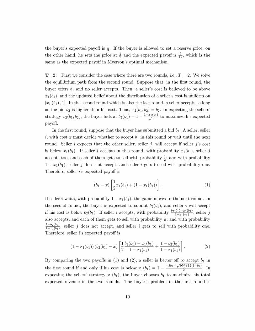
T=2: First we consider the case where there are two rounds, i.e., T = 2. We solve

the equilibrium path from the second round. Suppose that, in the �rst round, the

buyer o¤ers b1 and no seller accepts. Then, a seller�s cost is believed to be above

x1(b1), and the updated belief about the distribution of a seller�s cost is uniform on

[x1 (b1) ; 1]. In the second round which is also the last round, a seller accepts as long

as the bid b2 is higher than his cost. Thus, x2(b1; b2) = b2. In expecting the sellers�

strategy x2(b1; b2), the buyer bids at b2(b1) = 1� 1�x1(b1)p3

to maximize his expected

payo¤.

In the �rst round, suppose that the buyer has submitted a bid b1. A seller, seller

i, with cost x must decide whether to accept b1 in this round or wait until the next

round. Seller i expects that the other seller, seller j, will accept if seller j�s cost

is below x1(b1). If seller i accepts in this round, with probability x1(b1), seller j

accepts too, and each of them gets to sell with probability 12 ; and with probability

1 � x1(b1), seller j does not accept, and seller i gets to sell with probability one.Therefore, seller i�s expected payo¤ is

(b1 � x)�1

2x1(b1) + (1� x1(b1))

�: (1)

If seller i waits, with probability 1� x1(b1), the game moves to the next round. Inthe second round, the buyer is expected to submit b2(b1), and seller i will accept

if his cost is below b2(b1). If seller i accepts, with probabilityb2(b1)�x1(b1)1�x1(b1) , seller j

also accepts, and each of them gets to sell with probability 12 ; and with probability

1�b2(b1)1�x1(b1) , seller j does not accept, and seller i gets to sell with probability one.

Therefore, seller i�s expected payo¤ is

(1� x1(b1)) (b2(b1)� x)�1

2

b2(b1)� x1(b1)1� x1(b1)

+1� b2(b1)1� x1(b1)

�: (2)

By comparing the two payo¤s in (1) and (2), a seller is better o¤ to accept b1 in

the �rst round if and only if his cost is below x1(b1) = 1 ��3b1+

p9b21+12(1�b1)2 . In

expecting the sellers� strategy x1(b1), the buyer chooses b1 to maximize his total

expected revenue in the two rounds. The buyer�s problem in the �rst round is

10

Table 1: Equilibrium outcomes for T = 1; 2; 3; 4; 5:Buyer�s Payo¤ E (�) xT�4 xT�3 xT�2 xT�1 xT

(bT�4) (bT�3) (bT�2) (bT�1) (bT )

T = 1 0:38490 0 0:4225(0:4225)

T = 2 0:40024 0:2972 0:1709 0:5212(0:4214) (0:5212)

T = 3 0:40111 0:4563 0:0597 0:2165 0:5475(0:4099) (0:4538) (0:5475)

T = 4 0:40115 0:5826 0:0154 0:0597 0:2165 0:5475(0:4007) (0:4127) (0:4538) (0:5475)

T = 5 0:40115 0:6626 0:0070 0:0154 0:0597 0:2165 0:5475(0:3990) (0:4021) (0:4127) (0:4538) (0:5475)

de�ned as

maxb1[1� b1]

h1� (1� x1(b1))2

i+ [1� b2 (b1)]

h(1� x1 (b1))2 � (1� b2 (b1))2

i:

So, in equilibrium, b1 = 0:4214; b2 = 0:5212; x1 = 0:1709; x2 = 0:5212, and the

buyer�s payo¤ is 0:40024.

T=1�5: Table 1 shows the equilibrium paths of the cuto¤ xt and the bid bt, and

the buyer�s expected payo¤s when the number of rounds T = 1; 2; 3; 4; and 5.

Column E (�) lists the expected transaction time conditional on the transaction

occurring. We assume that the game begins at time 0 and ends at time 1. If the

buyer�s bid in the tth round is accepted, the transaction occurs at (t�1)T : There are

several points worth noting:

1. The cost cuto¤ in round T�� , xT�� , increases in T and converges when T goesto in�nity.1112 The buyer�s payo¤ increases in T , but the increment shrinks

as T increases. Therefore, the pro�t from having one more bidding chance

shrinks as T increases.

2. Given T , the cuto¤ path xt and the bidding path bt are increasing. With a

larger T , however, the rate of increase is small in the �rst few rounds, and

11The numerical results have four digits of precision, so the numbers in the table might not besu¢ ciently accurate to show small di¤erences.12This is proved in Lemma 1 in Appendix A.

11

large jumps occur in the last few rounds. This represents one class of the

equilibrium path. If we consider another example with v = 1:5, then the

sequence of xt when T = 5 becomes f0:1318; 0:2823; 0:4600; 0:6678; 0:9125g.This represents another class of the equilibrium path along which xt increases

steadily over time (as characterized in Theorem 1).

3. The payo¤ is lower than the payo¤ in a reverse auction with the optimal

reserve price for all values of T ; and when T is large enough (in this example,

when T � 1), the payo¤ is higher than the payo¤ in a reverse auction with noreserve price (as shown by Theorem 2).

4. In equilibrium, the buyer does not get the object only if both sellers� costs

are above xT . Therefore, the probability of the buyer getting the object in-

creases in T , but the increment shrinks as T increases. From the table, we see

that when T increases from 3 to 4, and to 5, neither the buyer�s payo¤ nor

the probability that the buyer gets the object increases much. However, the

expected transaction time is much later. This fact suggests that if the buyer

has waiting cost and prefers earlier transactions, having fewer rounds might

be good for him. The analysis in Section 5 con�rms the conjecture.

3 Derivation of the Equilibrium Path

In this section, we brie�y describe how we obtain the equilibrium path of this dy-

namic game and show its existence. The complete construction of the equilibrium

strategy and belief is shown in the online appendix.

First, let�F (x) = 1� F (x)

be the counter-cumulative distribution function. In the last round t = T , a seller

accepts the last-round bid bT as long as his cost is below bT , so the cost cuto¤

xT = bT . Knowing this, and given the belief that all the sellers have costs higher

than xT�1, the buyer chooses bT to maximize his payo¤:

VT (xT�1) = maxbT2[xT�1;c];xT

(v � bT )P (xT�1; xT )

s:t: bT = xT :

P (xT�1; xT ) � �F (xT�1)N � �F (xT )

N is the probability that all the sellers� costs

12

are above xT�1 and that the demand is ful�lled, given that sellers with costs be-

tween xT�1 and xT are willing to provide the good. The maximizers, bT (xT�1)

and xT (xT�1), are the buyer�s bid and the sellers�cost cuto¤ in the continuation

equilibrium given belief xT�1:�bT (xT�1) ; xT (xT�1)

�2 arg max

bT ;xT2[xT�1;c](v � bT )P (xT�1; xT ) (P1)

s:t: bT = xT :

Next we proceed backward to round t = T � 1. Given belief xt�1, suppose thatthe buyer chooses bt 2 [xt�1; c]. The cost cuto¤ xt in round t is determined by

�nding the type of seller who is indi¤erent between accepting in round t and round

t+ 1:

xt 2 � (bt; xt�1) �(x 2 [xt�1; c] j (bt � x)

G (xt�1; x)

NF (xt�1)N�1 =

Ct+1 (x)

NF (xt�1)N�1

); (3)

whereG (xt�1; x) �PN�1n=0

�F (x)N�1�n �F (xt�1)n and Ct+1 (x) = (bt+1 (x)�x)G (x; xt+1 (x)).Given belief xt�1,

G(xt�1;xt)

NF (xt�1)N�1 is the conditional probability that a seller with cost xt

gets to sell the good if he accepts in round t; Ct+1(xt)

NF (xt�1)N�1 and (bt�xt) G(xt�1;xt)

NF (xt�1)N�1 are

the expected payo¤s of a seller with cost xt if he accepts in round t+1 and in round

t, respectively. By expecting the other sellers to apply the cuto¤ strategy with cuto¤

xt 2 � (bt; xt�1), a seller with cost x gets expected payo¤s (bt+1 (xt)�x)G(xt;xt+1(xt))NF (xt�1)N�1

and (bt � x) G(xt�1;xt)

NF (xt�1)N�1 if accepting in round t+ 1 and in round t, respectively. In

comparing the two payo¤s, a seller is better o¤ by accepting bt in round t if and

only if his cost is below xt.13

By expecting (3), the buyer chooses bt (xt�1) to maximize his expected payo¤

13For some values of bt, � (bt; xt�1) in (3) might be empty. In the online appendix, we constructa continuation equilibrium for the case when � (bt; xt�1) is empty and show that choosing bt 2fb j � (b; xt�1) = �g is not an optimal strategy for the buyer. So, without loss of generality, we canfocus on bt 2 fb j � (b; xt�1) 6= �g when deriving the equilibrium path.

13

Vt (xt�1):

Vt (xt�1) = maxbt;xt2[xt�1;c]

(v � bt)P (xt�1; xt) + Vt+1 (xt)

s:t: (bt � xt)G (xt�1; xt) = Ct+1 (xt) ;�bt (xt�1) ; xt (xt�1)

�2 arg max

bt;xt2[xt�1;c](v � bt)P (xt�1; xt) + Vt+1 (xt) (P2)

s:t: (bt � xt)G (xt�1; xt) = Ct+1 (xt) :

Applying the same procedure backward, we obtain a sequence of bt (xt�1) and

xt (xt�1), for t = 1; 2; � � �T . However, we need to make sure that solutions to

(P1) and (P2) exist. This is proved in the following proposition. Note that there

might be multiple solutions to programs (P1) and (P2). In that case, only those

that ensure the existence of equilibrium can be candidates for bt (xt�1) and xt (xt�1)

(see the proof of Proposition 1 for more details).

Proposition 1 There exists a set of solutions�bt (xt�1) ; xt (xt�1)

tthat solves pro-

grams (P1) and (P2) for all t.

Sketch of Proof. The details of the proof are in Appendix A. Here is the outline.

First, by Berge�s maximum theorem, VT (xT�1) is continuous, and the solution set

of xT for program (P1) is upper hemi-continuous. Therefore, we are able to pick

xT (xT�1) from the solution set such that CT (xT�1) is lower semi-continuous. Next,

by substituting the constraint into the objective function in round T �1 in program(P2), the objective function is graph-continuous as de�ned in Leininger (1984),

and by Leininger�s generalized maximum theorem, VT�1 is upper semi-continuous,

and the solution set of xT�1 exists and is upper hemi-continuous. Applying the

same procedure backward, we guarantee the existence of a solution to each round-t

program.

The following remark summarizes the procedure adopted to derive the equilib-

rium path:

Remark 1 The equilibrium path f(b1; � � � ; bT ) ; (x1; � � � ; xT )g can be found by solv-ing the recursive program

Vt (xt�1) = maxbt;xt2[xt�1;c]

(v � bt)P (c; xt) + Vt+1 (xt) (P3)

s:t: (bt � xt)G (xt�1; xt) = Ct+1 (xt) ;

14

where x0 = c, VT+1 (xT ) = 0, and CT+1 (xT ) = 0. The value of the program with

t = 1 is the buyer�s payo¤ in equilibrium.

Program (P3) shows that the equilibrium path f(b1; � � � ; bT ) ; (x1; � � � ; xT )g max-imizes the buyer�s payo¤ subject to two constraints. The �rst one is the sellers�

incentive-compatibility constraint, which ensures that sellers with di¤erent values

will not deviate from their equilibrium choices. This constraint exists in every mech-

anism and is shown in the constraint part of the program. The second constraint is

the buyer�s inability to commit to a bidding path over time, which amounts to the

recursive form of the program where the buyer utilizes all of the available informa-

tion to set a bid in each round. While this allows the buyer to adopt the ex post

optimal strategy, the lack of commitment on his part changes the prices that a seller,

who expects the buyer�s strategy correctly, is willing to accept in early rounds, and

hence prevents the buyer from achieving the ex ante optimal outcome derived in

Myerson (1981).

4 Equilibrium Bidding Behavior with No Lockout Pe-

riod

In this section, we analyze the equilibrium bidding path when there is no lockout

period so that the buyer can submit as many bids as desired, i.e., T !1. Two ofour main results are established here. First, we characterize the equilibrium bidding

path and show that any equilibrium can be classi�ed into one of the following two

classes: (i) a fully screening equilibrium and (ii) a price ceiling equilibrium. Second,

we show that without a lockout period, the expected payo¤ of a buyer is weakly

higher than that in a reverse auction without a reserve price, but lower than that

in a reverse auction with the optimal reserve price.

4.1 Commitment and optimality

Before proceeding to the main result, we �rst consider the benchmark case where

the buyer can commit to a bidding path in advance. We characterize the optimal

path under commitment and show that, without commitment, Myerson�s optimal

outcome for the buyer might not be attainable, even though the buyer can adjust

the bid as frequently as he likes.

15

In our setting, a reverse Dutch auction with a reserve price r such that r+ Fi(r)fi(r)

=

v implements Myerson�s optimal mechanism.14 In such a reverse Dutch auction,

the price is continuously increased and stops at the reserve price. Therefore, if

the buyer can commit and the number of rounds is large enough, the buyer can

roughly duplicate the price path in a reverse Dutch auction and receive a payo¤

approximately the same as in an optimal mechanism.

Nonetheless, when commitment is not possible, the maximum payo¤ resulting

from the optimal mechanism is not approximately achievable if the optimal auction

design involves setting a reserve price. To see this, recall that on the equilibrium

path, the last-round bT and xT can be found by solving

xT = bT = argmaxb(v � b)

h�F (xT�1)

N � �F (b)Ni:

A necessary condition for bT is

�F (xT�1)N = �F (bT )

N + (v � bT )N �F (bT )N�1 f (bT ) : (4)

Suppose that the optimal auction involves setting a reserve price r < c. If the

optimal auction can be approximately implemented when T goes to in�nity, then it

must be that limT!1 bT = limT!1 xT = r and limT!1 xT�1 = r. Nevertheless,

by equation (4), if limT!1 bT = r, limT!1 xT�1 < r, so that the optimal auction

cannot be approximately implemented.

4.2 Characterization of the equilibrium paths

In characterizing the equilibrium path, the key question is how the buyer designs the

bidding path to screen out the sellers. When it is possible to commit to the entire

bidding path, it is optimal for the buyer to di¤erentiate the sellers by gradually

raising the bid. However, this strategy of �nely screening out the sellers may not be

optimal when the buyer is unable to commit, as he would inevitably react to any

new information that can be gained along the way. We show that, in general, all

the possible equilibrium paths can be classi�ed into two classes: either the sellers

with di¤erent costs are almost fully separated so the sellers�private information is

revealed gradually over time, or they are pooled into several cost intervals and most

information about the sellers�costs is revealed just before the deadline.

14 If v � c+ 1fi(c)

, no reserve price is required to implement the optimal mechanism.

16

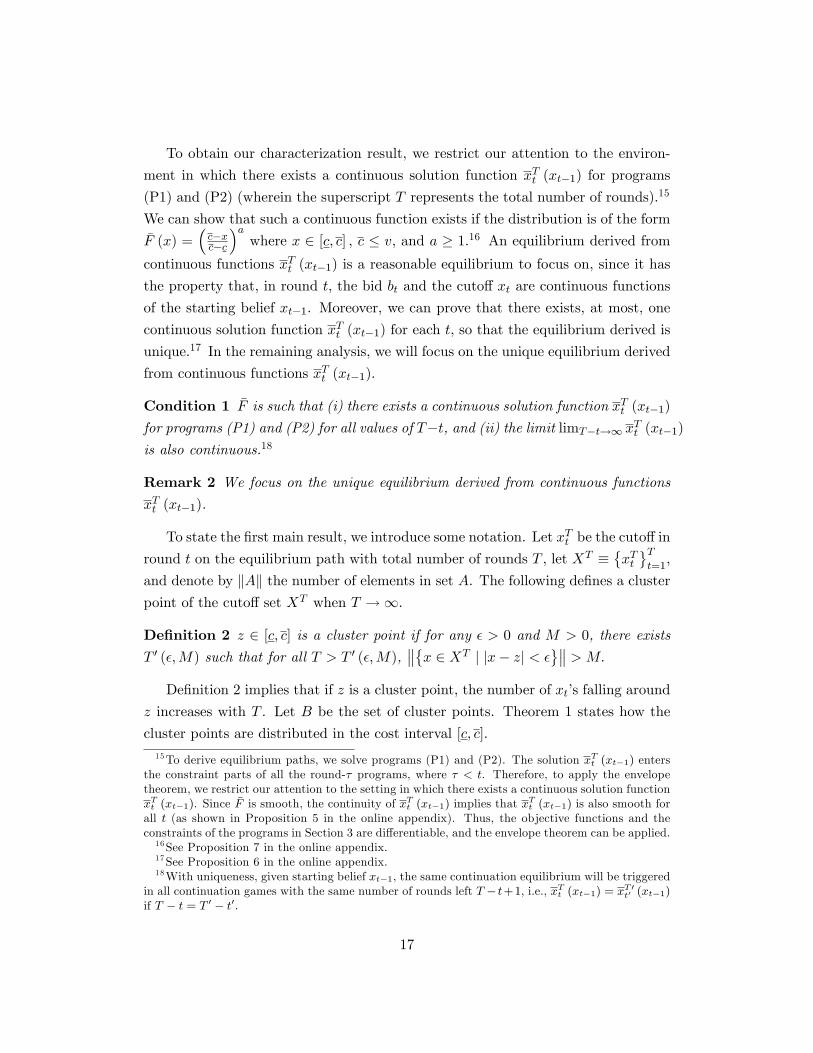
To obtain our characterization result, we restrict our attention to the environ-

ment in which there exists a continuous solution function xTt (xt�1) for programs

(P1) and (P2) (wherein the superscript T represents the total number of rounds).15

We can show that such a continuous function exists if the distribution is of the form�F (x) =

�c�xc�c

�awhere x 2 [c; c] ; c � v; and a � 1.16 An equilibrium derived from

continuous functions xTt (xt�1) is a reasonable equilibrium to focus on, since it has

the property that, in round t, the bid bt and the cuto¤ xt are continuous functions

of the starting belief xt�1. Moreover, we can prove that there exists, at most, one

continuous solution function xTt (xt�1) for each t, so that the equilibrium derived is

unique.17 In the remaining analysis, we will focus on the unique equilibrium derived

from continuous functions xTt (xt�1).

Condition 1 �F is such that (i) there exists a continuous solution function xTt (xt�1)

for programs (P1) and (P2) for all values of T�t, and (ii) the limit limT�t!1 xTt (xt�1)is also continuous.18

Remark 2 We focus on the unique equilibrium derived from continuous functions

xTt (xt�1).

To state the �rst main result, we introduce some notation. Let xTt be the cuto¤ in

round t on the equilibrium path with total number of rounds T , let XT ��xTtTt=1,

and denote by kAk the number of elements in set A. The following de�nes a clusterpoint of the cuto¤ set XT when T !1.

De�nition 2 z 2 [c; c] is a cluster point if for any � > 0 and M > 0, there exists

T 0 (�;M) such that for all T > T 0 (�;M), �x 2 XT j jx� zj < �

> M:De�nition 2 implies that if z is a cluster point, the number of xt�s falling around

z increases with T . Let B be the set of cluster points. Theorem 1 states how the

cluster points are distributed in the cost interval [c; c].15To derive equilibrium paths, we solve programs (P1) and (P2). The solution xTt (xt�1) enters

the constraint parts of all the round-� programs, where � < t. Therefore, to apply the envelopetheorem, we restrict our attention to the setting in which there exists a continuous solution functionxTt (xt�1). Since �F is smooth, the continuity of xTt (xt�1) implies that x

Tt (xt�1) is also smooth for

all t (as shown in Proposition 5 in the online appendix). Thus, the objective functions and theconstraints of the programs in Section 3 are di¤erentiable, and the envelope theorem can be applied.16See Proposition 7 in the online appendix.17See Proposition 6 in the online appendix.18With uniqueness, given starting belief xt�1, the same continuation equilibrium will be triggered

in all continuation games with the same number of rounds left T � t+1, i.e., xTt (xt�1) = xT 0t0 (xt�1)if T � t = T 0 � t0.

17

Theorem 1 Assume Condition 1.

1. The cluster point set B is either the whole interval [c; c] or a single point fcg,i.e., B = [c; c] or fcg.

2. The cluster point set B is a single point fcg if and only if the last periodcuto¤ xTT is bounded away from c when T ! 1, i.e., B = fcg if and only iflimT!1 x

TT < c:

3. If B = [c; c], the buyer�s payo¤ is approximately the same as that in a reverse

auction without a reserve price.

Sketch of Proof. The details of the proof are in Appendix A. Here is the sketch.

We �rst show that if the number of rounds left in a continuation game starting with

belief xt�1 goes to in�nity, then the di¤erence between xt and xt�1 goes to zero. So,

if a 2 [c; c] is a cluster point, any point x < a must be a cluster point, too. However,we can also show that it cannot be the case wherein a 2 (c; c), [c; a] belongs to thecluster point set B, and (a; c] belongs to the complement of B because such a path

implies that the buyer does not choose the optimal strategy in a certain round, and

thus cannot be an equilibrium path. Therefore, the cluster point set is either [c; c]

or fcg. The third statement follows from the revenue equivalence theorem.

The theorem states that any equilibrium can be classi�ed into either one of the

two classes, each of which exhibits di¤erent properties and o¤ers di¤erent implica-

tions. For expositional purposes, we refer to the equilibrium with the cluster point

set [c; c] as the fully screening equilibrium and refer to the equilibrium with the

cluster point set fcg as the price ceiling equilibrium. To see why these two classes ofpaths arise in equilibrium, notice that in our setting, a reverse Dutch auction with

the optimal reserve price implements Myerson�s optimal mechanism: if the buyer

can commit, it is in his best interest to commit to a strategy in which he gradually

raises the bid to fully price discriminate among the sellers until it reaches the opti-

mal reserve price. This is not implementable, however, when the buyer is unable to

commit to a bidding path because he cannot avoid responding to the information

revealed by sellers�rejections. To commit to a price ceiling, therefore, it is impera-

tive to ensure that the buyer does not gain much information from rejections, which

can be achieved by keeping the bids low enough because rejecting a low bid does

not reveal much about the sellers�costs. With the lack of commitment, the buyer

18

thus faces a cumbersome trade-o¤: on the one hand, he would like to raise the bid

gradually to better screen out the sellers; on the other hand, he also needs to keep

the bids low enough not to gain much information to respond to. If the bene�t of

having a price ceiling dominates the bene�t of �ne screening, the buyer will keep

the bids su¢ ciently low in initial rounds, followed by large jumps at the end to the

reserve price; if not, the buyer will increase the bid steadily over time until it reaches

the upper bound c.

The distribution of the cluster points also indicates several notable properties of

each class of equilibrium. First, in the fully screening equilibrium where the cluster

point set spans over the whole interval [c; c], the cuto¤s are more evenly distributed

over the interval. The sellers are more �nely screened as the number of rounds T

increases, and fully separated in the limit. Information is revealed more gradually

over time, and a transaction is more likely to occur earlier than in the price ceiling

equilibrium.

By contrast, in the price ceiling equilibrium where the cluster point set is a single

point fcg, while the number of cuto¤s falling in interval [c; c+ �) for an arbitrarilysmall � increases with T , the number falling in [c+ �; c] does not. Only those sellers

with costs arbitrarily close to c are more �nely separated, but all other types are

roughly partitioned into a �nite number of groups. Most information is revealed

in the last few rounds, but in a rough manner because those remaining sellers are

partially pooled, even in the limit. This also means that most types accept in the

last few rounds, and a transaction is more likely to occur late. Moreover, since the

bids are kept low in initial rounds followed by large discrete jumps at the end, the

bidding path is convexly increasing. By doing so, the buyer can successfully commit

to a price ceiling, i.e., limT!1 xTT < c.

These properties of the price ceiling equilibrium seem to capture important facets

of real bargaining situations well. Spann and Tellis (2006) analyze bidding patterns

in the data of a NYOP retailer in Germany that sells airline tickets for various airlines

and allows multiple bidding. They argue that: (i) with a positive bidding cost, the

pattern should be concavely increasing, because at the beginning consumers try to

increase the probability of successful bidding by bidding higher, but when the bids

are closer to their reservation value, the rate of increase slows down; (ii) with zero

bidding cost, the pattern should be linearly increasing. They �nd, however, that

only 36% of the data �t the �rst pattern (concavely increasing) and 5% �t the second

pattern (linearly increasing). Moreover, they even �nd that 23% of the data �t the

19

pattern which is convexly increasing, prompting them to conclude that consumer

behavior on the Internet is not so rational. Our analysis provides an explanation

for this seemingly puzzling observation, i.e., a convexly increasing bidding path can

actually occur in a fully rational environment. In addition to this, in the price

ceiling equilibrium, a transaction is more likely to occur in the last few rounds.

This is related to the deadline e¤ect that has been observed in many negotiation

processes such as bargaining during strikes and pretrial negotiations.

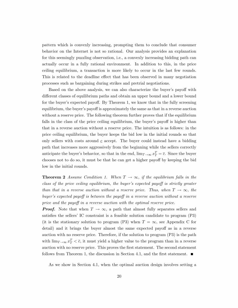
Based on the above analysis, we can also characterize the buyer�s payo¤ with

di¤erent classes of equilibrium paths and obtain an upper bound and a lower bound

for the buyer�s expected payo¤. By Theorem 1, we know that in the fully screening

equilibrium, the buyer�s payo¤ is approximately the same as that in a reverse auction

without a reserve price. The following theorem further proves that if the equilibrium

falls in the class of the price ceiling equilibrium, the buyer�s payo¤ is higher than

that in a reverse auction without a reserve price. The intuition is as follows: in the

price ceiling equilibrium, the buyer keeps the bid low in the initial rounds so that

only sellers with costs around c accept. The buyer could instead have a bidding

path that increases more aggressively from the beginning while the sellers correctly

anticipate the buyer�s behavior, so that in the end, limT!1 xTT = c. Since the buyer

chooses not to do so, it must be that he can get a higher payo¤ by keeping the bid

low in the initial rounds.

Theorem 2 Assume Condition 1. When T ! 1, if the equilibrium falls in the

class of the price ceiling equilibrium, the buyer�s expected payo¤ is strictly greater

than that in a reverse auction without a reserve price. Thus, when T ! 1, thebuyer�s expected payo¤ is between the payo¤ in a reverse auction without a reserve

price and the payo¤ in a reverse auction with the optimal reserve price.

Proof. Note that when T ! 1, a path that almost fully separates sellers andsatis�es the sellers�IC constraint is a feasible solution candidate to program (P3)

(it is the stationary solution to program (P3) when T = 1, see Appendix C for

detail) and it brings the buyer almost the same expected payo¤ as in a reverse

auction with no reserve price. Therefore, if the solution to program (P3) is the path

with limT!1 xTT < c, it must yield a higher value to the program than in a reverse

auction with no reserve price. This proves the �rst statement. The second statement

follows from Theorem 1, the discussion in Section 4.1, and the �rst statement.

As we show in Section 4.1, when the optimal auction design involves setting a

20

reserve price, the inability to commit to a bidding path prevents the buyer from

achieving the outcome derived from Myerson�s optimal mechanism, which can be

implemented by a reverse auction with the optimal reserve price. However, the

presence of a deadline endows the buyer with certain commitment power and thus

enables the buyer to achieve a payo¤ higher than in a reverse auction without any

reserve price.

4.3 Factors in determining the class of the equilibrium path

Which class of equilibrium would occur depends on the distribution of the sellers�

cost �F , the buyer�s value v, and the number of sellers N , parameters that a¤ect

the buyer�s trade-o¤ between �nely screening the sellers�costs and having a reserve

price. With a higher v, the buyer values the good more highly and cannot stand the

risk of not getting the good, so setting a reserve price is less pro�table for the buyer.

On the other hand, when N is larger, the probability that there exists a seller with

a low cost increases, and competition among the sellers forces them to accept lower

prices, too, so that a buyer also bene�ts less from setting a reserve price. We know

that if the bene�t of screening �nely dominates the bene�t of having a reserve price,

the fully screening equilibrium arises. Therefore, we expect that the fully screening

equilibrium is more likely to occur when v is large and when N is large.19

The relationship between v and the class of the equilibrium path is illustrated

in Figure 1. Figure 1 shows the path of xt for di¤erent values of v when T = 20;

N = 2, and a seller�s cost is uniformly distributed on [0; 1]. With v = 1; v = 1:2; and

v = 1:4, the optimal reserve prices are 0:5; 0:6; and 0:7, respectively. So when v = 1,

the buyer is more inclined to have xT much lower than c = 1, and the price ceiling

equilibrium arises; in equilibrium, a seller with a cost higher than 0:1 will not sell

the good until the last two rounds, which implies that transactions are much more

likely to occur in the last two rounds. On the other hand, when v = 1:4, the loss

from having xT much lower than c = 1 dominates the bene�t, so the fully screening

equilibrium arises; in equilibrium, the buyer raises bids gradually to a price close to

1, and a transaction is almost equally likely to occur in every round. The result that

the fully screening equilibrium is more likely to occur when v is large is formally

proved in Proposition 2.

19The intuition regarding how N a¤ects the equilibrium path is con�rmed in Horner and Samuel-son (2011). They prove that when v = 1 and a seller�s cost is uniformly distributed on [0; 1], anequilibrium path with limT!1 x

TT < c occurs if and only if N < 6.

21

0 2 4 6 8 10 12 14 16 18 200

0.1

0.2

0.3

0.4

0.5

0.6

0.7

0.8

0.9

1

xt

t

v=1v=1.2v=1.4

Figure 1: Path of xt

Proposition 2 Assume Condition 1. There exists a threshold �v such that the priceceiling equilibrium occurs if and only if v < �v.

Proof. In round T � 1, given v and belief xT�2, the buyer�s payo¤ is

VT�1 (xT�2; v) = (v � xT�1 (xT�2; v))h�F (xT�2)

N � �F (xT�1 (xT�2; v))Ni

�CT (xT�1 (xT�2; v))��F (xT�2)� �F (xT�1 (xT�2; v))

�+ VT (xT�1 (xT�2; v) ; v) ;

where VT�1 (xT�2; v) and xT�1 (xT�2; v) are as de�ned in (P2) but with one more

argument v. By the envelope theorem, @VT�1@v =��F (xT�2)

N � �F (xT�1)N�+ @VT

@v ,

where @VT@v = �F (xT�1)N � �F (xT )

N , so @VT�1@v = �F (xT�2)

N � �F (xT )N . For clari�ca-

tion, given v, let xTT (v) be the equilibrium cuto¤ in round T , and �T (v) and � (v)

be the buyer�s payo¤s in our model with T rounds and in a reverse auction without

a reserve price, respectively. Applying similar procedures to derive @VT�2@v , @VT�3@v ,

� � � , we can conclude that d�T (v)dv = 1� �F

�xTT (v)

�N � 1. Note that d�dv = 1.We next show that it cannot be the case that for v0 > v, limT!1 xTT (v

0) < c and

limT!1 xTT (v) = c. If that is the case, by Theorem 2, limT!1 �T (v0) > � (v0) and

22

limT!1 �T (v) = � (v).

limT!1

�T (v) = limT!1

�T�v0��Z v0

v

d limT!1 �T (x)

dxdx (5)

and

� (v) = ��v0��Z v0

v

d� (x)

dxdx: (6)

Since limT!1 �T (v0) > � (v0) andd limT!1 �T (x)

dx � d�(x)dx , by (5) and (6), limT!1 �T (v) >

� (v), a contradiction. Therefore, there is a threshold �v such that limT!1 xTT (v) < c,

i.e., the price ceiling equilibrium occurs, if and only if v < �v.

5 The Role of the Lockout Period

In this section, we extend the model to consider the situation in which the buyer

discounts the future, i.e., the buyer wants to close the transaction as early as pos-

sible.20 We show that with discounting, setting an appropriate lockout period rule

may bene�t the buyer, and we use numerical examples to examine the conditions

under which having a lockout period bene�ts the buyer.

5.1 Model with discounting

The model is modi�ed as follows. The buyer realizes his demand for the good at

time 0 and tries to ful�ll the demand in time period [0;M ]. After time M , the

buyer no longer needs the good. If the buyer gets the good at price B at time t,

his utility is �tM (v �B), where � 2 (0; 1) is the discount factor for the whole time

period [0;M ]. A lockout period rule is set to regulate how frequently the buyer can

submit a bid. If the lockout period is s, the buyer can submit bids for bMs c times,that is, T = bMs c.

With discounting, the buyer is more anxious to close the transaction early, but

the buyer�s trade-o¤ between �nely screening the sellers�costs and successfully com-

mitting to a reserve price still exists. If the buyer tries to commit to a reserve price,

he has to bear the cost of delaying the transaction as well as not being able to screen

the sellers. On the contrary, if the buyer gives up having a reserve price, he can

raise the bid aggressively to close the transaction; moreover, if the buyer can revise

20We continue to assume that the sellers have no preference for early or late transactions.

23

0 5 10 15 20 25 30 35 40 45 500

0.1

0.2

0.3

0.4

0.5

0.6

0.7

0.8

0.9

1

t

xt

delta=.30delta=.80delta=.95delta=1

Figure 2: Path of xt with di¤erent values of �

his bids extremely frequently, the sellers�costs can be �nely screened in a minute.

Example 1 To see how � a¤ects the equilibrium path, Figure 2 shows the paths

of xt for di¤erent values of � when v = 1, T = 50, N = 2, and a seller�s cost is

uniformly distributed on [0; 1]. We can see that with lower �, the path becomes

more concave, and a trade is more likely to occur in early rounds. This is consistent

with our intuition because a buyer with a lower � (who discounts the future more

heavily) will �nd delaying the transaction to commit to a reserve price more costly,

and hence will choose to raise bids aggressively.

Summary of Example 1 A buyer with a lower � raises bids more aggressively,

and the equilibrium path of xt becomes more concave.

5.2 Examples for the optimal lockout period

When there is no discounting, having more rounds does not hurt the buyer because

the buyer can choose to waste the additional bidding chances in the beginning.

However, this strategy postpones the trade and cannot be implemented without

24

cost when the buyer discounts the future. Therefore, with a discount factor � < 1,

the buyer�s payo¤might not monotonically increase with the number of rounds, and

setting a lockout period might increase the buyer�s payo¤.

We use numerical examples to illustrate the circumstances under which having

a lockout period bene�ts the buyer. We consider scenarios with di¤erent values

of � and N , and summarize the results of the numerical examples in Summary of

Example 2 and Summary of Example 3. Notice that we focus on the environment

in which Myerson�s optimal mechanism involves setting a reserve price. If setting a

reserve price is unnecessary, having more rounds always bene�ts the buyer because

it helps the buyer to separate the sellers better and to close the transaction earlier.

Example 2 Suppose that N = 2; v = 1:2; and a seller�s cost is uniformly dis-

tributed on [0; 1] : We consider the cases with � = 1, 0:96, 0:9, and 0:85, and the

results are shown in the following table. The second column of the table shows the

cost cuto¤ in the last round when T goes to in�nity.21 When � = 0:9 and 0:85,

limT!1 xT = 1, so the buyer raises the bid aggressively to c from the beginning,

and the equilibrium paths of xt are concave. The third column shows the number of

rounds T � that maximizes the buyer�s payo¤, and the corresponding buyer�s payo¤

given T � is shown in the last column.22

� limT!1 xT T � � (T �)

1:00 0:680 1 0:5556

0:96 0:808 3 0:5473

0:90 1 2 0:5399

0:85 1 1 0:5333

The result shows that when � = 0:96 and 0:9, setting a lockout period to allow

the buyer to bid three and two times respectively maximizes the buyer�s payo¤.

With � = 0:96, when there is no lockout period, limT!1 xT < 1, so the equilibrium

path of xt is mostly convex, and the transaction is very likely to occur late. This is

21We derive the results numerically, so T cannot increase unboundedly. However, we check allthe cases when T � 1000 and �nd that the last-round cuto¤s xT are constant for T � 25.22We know that for � = 1, the buyer�s payo¤ increases with T . For � = 0:96, 0:9, and 0:85,

although we do not derive the buyer�s payo¤s when T goes to in�nity, we check how the payo¤schange when T increases from 1 to 1000. For � = 0:96, when T � 10, the payo¤ falls below 0:54and shows a trend of decline in T . For � = 0:9 and 0:85, the payo¤s show a trend of increase whenT is large enough, and since limT!1 xT = 1, the payo¤s converge to the payo¤ in a reverse auctionwith no reserve price.

25

illustrated by the dotted line in Figure 3, which shows the cuto¤ path when there

are 50 rounds. The three stars in Figure 3 represent the equilibrium path when

there are only 3 rounds. By comparing the two paths, we can see that by setting

a lockout period so that the buyer is allowed to bid three times, the buyer bene�ts

from having early transactions but su¤ers from not being able to separate sellers

with costs around c. When � = 1, limT!1 xT < 1 as well, so the pros and cons

of a lockout period rule are similar. However, waiting is more costly in the case

of � = 0:96 than in the case of � = 1. Therefore, when � = 0:96, the bene�t of

setting an appropriate lockout period dominates the loss; but when � = 1, the loss

dominates the bene�t.

With � = 0:9, when there is no lockout period, limT!1 xT = 1, so the equilib-

rium path of xt is concave, and transactions occur early. This is illustrated by the

dotted line in Figure 4, which shows the cuto¤ path when there are 50 rounds. The

two stars in Figure 4 represent the equilibrium path when there are only 2 rounds.

We can observe that, by setting a lockout period, the buyer bene�ts from having a

last-round bid lower than c, which functions like a reserve price, but su¤ers from not

being able to close the transaction early and separate sellers �nely. When � � 0:85,limT!1 xT = 1 as well, so the pros and cons of the lockout period rule are similar.

Since waiting is more costly when � is smaller, the loss caused by not being able to

close the transaction early dominates the bene�t when � � 0:85, while the bene�tdominates the loss when � = 0:9. The example thus indicates that the buyer bene�ts

from setting an appropriate lockout period when � is in the middle range.

Summary of Example 2 Setting an appropriate lockout period increases the buyer�spayo¤ when � is in the middle range.

In addition to the situation mentioned above, if having a reserve price is valuable

for the buyer (so that even with only one bidding chance allowed and no other chance

to screen the sellers, the buyer still gets a higher payo¤ than in a reverse auction

with no reserve price), then setting an appropriate lockout period bene�ts the buyer

when � is not too large. For instance, consider the case where v = 1; N = 2; and

a seller�s cost is uniformly distributed on [0; 1]. The optimal reserve price is 0:5.

Having a reserve price can improve the buyer�s payo¤ greatly. When � is lower than

0:62, limT!1 xT = 1, so that the buyer�s payo¤ when there is no lockout period

is at most 13 (the payo¤ in a reverse auction with no reserve price). On the other

hand, the buyer�s payo¤ when only one bidding chance is allowed is 0:3849 for all

26

0 5 10 15 20 25 30 35 40 45 500

0.1

0.2

0.3

0.4

0.5

0.6

0.7

0.8

0.9

Figure 3: Path of xt when there are 50 rounds and when there are 3 rounds, � = 0:96.

0 5 10 15 20 25 30 35 40 45 500.1

0.2

0.3

0.4

0.5

0.6

0.7

0.8

0.9

1

t

xt

Figure 4: Path of xt when there are 50 rounds and when there are 2 rounds, � = 0:9.

27

�. Therefore, when � < 0:62, setting an appropriate lockout period always bene�ts

the buyer.

Example 3 Suppose that v = 1, � = 0:95, and a seller�s cost is uniformly distrib-

uted on [0; 1] : We consider the cases with N = 2, 3, and 4, and as in the previous

example, the following table shows the limit of the last round cuto¤ when T goes

to in�nity limT!1 xT , the number of rounds that maximizes the buyer�s payo¤ T �,

and the corresponding buyer�s payo¤ � (T �).23

N limT!1 xT T � � (T �)

2 0:630 2 0:3949

3 0:917 4 0:5065

4 1 1 0:6000

The result shows that when the number of sellers is 2 or 3, setting an appropriate

lockout period so that the buyer has only a few bidding chances increases the buyer�s

payo¤; however, if the number of sellers is larger than 3, having more rounds is better

for the buyer. The reasoning is as follows. As we discussed in Section 4.3, when

N is large, having a reserve price does not increase the buyer�s payo¤ much, so

without a lockout period, the buyer does not hesitate to raise the bid from the

beginning. Therefore, limT!1 xT = 1, the equilibrium path of xt is concave, and

transactions occur early. Similar to what is shown in Figure 4, by setting a lockout

period, the buyer bene�ts from having a last-round bid lower than c, which functions

like a reserve price, but su¤ers from not being able to close the transaction early

and separate sellers �nely. However, when N is large, having a reserve price is not

important to the buyer, so that the loss dominates the bene�t, and the buyer is

better o¤ without a lockout period.

Summary of Example 3 Setting a lockout period increases the buyer�s payo¤ whenN is small.

The above discussion shows that the optimal lockout period varies with the

environment. An appropriate lockout period increases the buyer�s payo¤ when the

23We derive the last-round cuto¤s and the payo¤s numerically when T increases from 1 to 1200.For N = 2, the cuto¤ and the payo¤ converge to 0:63 and 0:3834, respectively; and for N = 3, thecuto¤ and the payo¤ converge to 0:917 and 0:5, respectively. For N � 4, the cuto¤ converges to 1,and the payo¤ converges to the payo¤ in a reverse auction with no reserve price.

28

number of sellers is small and when the buyer�s discount factor is in the middle

range. Priceline�s lockout period rule seems to hurt customers by restricting their

rebidding opportunities, but in fact, a customer with waiting costs might �nd it

bene�cial.

6 Conclusion and Discussion

This paper analyzes the Name Your Own Price (NYOP) mechanism adopted by

Priceline. We characterize the buyer�s and the sellers� equilibrium strategies and

show that Priceline�s lockout period restriction, a design alleged to protect sellers,

can actually bene�t customers with moderate discount factors. The analysis also

suggests why, in reality, bargaining parties often take measures to make their o¤ers

rigid and consequently force themselves to make fewer o¤ers, and why last-minute

deals have become more prevalent with the advent of the Internet.

We show that when there is no lockout period and no waiting cost, the equilibria

can be classi�ed into two classes: (i) a fully screening equilibrium and (ii) a price

ceiling equilibrium. In the fully screening equilibrium, sellers with di¤erent costs are

almost fully separated with information about the sellers�cost revealed gradually

over time. In this case, the buyer raises bids continuously, ending, if necessary, with

a price equal to the highest possible cost c. In this equilibrium, which is e¢ cient, the

buyer�s payo¤ is approximately the same as the payo¤ in a reverse auction without

a reserve price. In the price ceiling equilibrium, while sellers with costs arbitrarily

close to the minimum cost level are �nely separated, all other types of sellers are

roughly partitioned into a �nite number of groups, and information about the sellers�

costs is barely revealed in the initial rounds. In this case, the buyer does not raise the

bid much until the very end, the ending bid is lower than c, and the buyer�s payo¤

is greater than the payo¤ in a reverse auction without a reserve price. In the price

ceiling equilibrium, most transactions occur just before the deadline. The delay of

transactions incurs waiting cost if the buyer discounts the future. Therefore, setting

a lockout period might actually bene�t a buyer by moving transactions forward.

Discussion on the modeling approach and Priceline�s mechanism As in

many other applied papers, our model is an abstraction of the real world, so it

misses many features of reality. First of all, the buyer�s value is probably not

known by the sellers. In reality, however, the information seems less imperfect

29

than the information about the sellers�costs (the lowest prices they are willing to

accept), which depend on the amounts of the excess inventory left over from their

traditional retail channels. Therefore, while assuming that the sellers� costs are

private information, we assume that the buyer�s valuation is publicly known. This

assumption also allows us to get around the signaling issue and focus on how the

bidding path is designed to elicit the sellers�information.

Next, although Priceline classi�es hotels into di¤erent star ratings to ease cus-

tomers� quality concerns when buying through NYOP, there might still be some

diversity within the same rating class. Hence, a customer might worry about the

adverse selection problem, that is, if he bids low, only those whose quality is at

the low end will accept. The adverse selection problem might increase a customer�s

starting bid as well as add twists to the subsequent bidding path. By accounting for

the quality dimension, as suggested in the procurement literature (see, e.g., Manelli

and Vincent (1995), Morand and Thomas (2002), and Asker and Cantillon (2010)),

a more sophisticated trading procedure might be necessary to increase the total

surplus and possibly achieve full e¢ ciency. This can explain why we have recently

seen o¤er-counter-o¤er negotiation mechanisms arising on eBay and iO¤er.com.

Extensions This paper indicates several interesting directions for future research.

In addition to the adverse selection problem indicated previously, based on our

analysis, one might be curious about whether Priceline could do better by adopting

other measures, such as restricting the number of bidding chances instead of the

frequency of bidding. Moreover, one might extend the model to consider the cases

where the buyer has private information and where there are multiple buyers bidding

at the same time. The following are some of our conjectures about the equilibrium

path in such extended circumstances.

When the buyer�s value is private information, signaling issues arise. Since types

with lower value are more inclined to bid low and have xT lower than c, if sellers

know that the buyer is of a lower type, they will accept lower prices. Knowing this,

high types might try to imitate low types, and low types might try to bid lower in

order to be distinguished from high types. Therefore, a convexly increasing path is

still likely to occur, and the lockout period rule might still bene�t the buyer.

When there are multiple buyers bidding at the same time (but the number of

sellers is still larger than the number of buyers), everyone will try to get a unit from

the seller with the lowest cost �rst. In the beginning, competition among the buyers

30

raises the price higher than it would have been if there were only one buyer, and

the sellers also raise the price thresholds that they are willing to accept. Once a

buyer�s o¤er is accepted by a seller, both leave the market, and the price drops to

a new level. Note that the price drops suddenly and is lower than it would have

been if no buyer had obtained a unit, which also means that the remaining sellers

are willing to accept a lower price after a buyer and a seller leave the market. This

is because the remaining sellers have rejected all prices o¤ered before, so all players

believe that the remaining units will be sold at higher costs; if at the same time,

the sellers asked for a higher price after a buyer had left, then the remaining buyers

would have to pay an even higher price. This would make the buyers try harder

to get the �rst unit, and the prices in the beginning would be driven up further.

Therefore, along the equilibrium path, when there are more buyers staying in the

market, the sellers ask for higher prices but the units sold are provided by sellers

with lower costs; and when fewer buyers are left in the market, the sellers ask for

lower prices and the units are sold by sellers with higher costs. This is an interesting

phenomenon waiting for future theoretical and empirical investigation.

Exploring these extensions will bring us one step closer to reality and a bet-

ter understanding of the NYOP mechanism as well as other bargaining and price

determination processes.

A Appendix: the proofs

In this Appendix, we provide the proofs of Proposition 1 and Theorem 1.

Proof of Proposition 1. In the last round, recall that

VT (xT�1) = maxxT2[xT�1;c]

(v � xT )P (xT�1; xT ) ;

xT (xT�1) 2 XT (xT�1) = arg maxxT2[xT�1;c]

(v � xT )P (xT�1; xT ) ;

and CT (xT�1) = (xT (xT�1)� xT�1)G (xT�1; xT (xT�1)) :

By Berge�s maximum theorem, we know that VT (xT�1) is continuous andXT (xT�1)

31

is upper hemi-continuous. In round t; t < T; let

�t (xt�1; xt) = (v � xt)h�F (xt�1)

N � �F (xt)Ni

�Ct+1 (xt)��F (xt�1)� �F (xt)

�+ Vt+1 (xt) ;

� (xt�1) = [xt�1; c] :

Then

Vt (xt�1) = maxxt2�(xt�1)

�t (xt�1; xt) ;

xt (xt�1) 2 Xt (xt�1) = arg maxxt2�(xt�1)

�t (xt�1; xt) :

We show that by picking a proper xt (xt�1) from Xt (xt�1) ; t � T , each round-t

program has a solution.

First, observe that for the upper hemi-continuous correspondence XT , we are

able to �nd (i) nT closed intervals [ak; ak+1] ; k = 1; � � � ; nT ; such that [k [ak; ak+1] =[c; c], and (ii) nT continuous functions xT;k : [ak; ak+1]! [ak; c] ; k = 1; � � � ; nT ; suchthat xT;k (x) 2 XT (x) ;8x 2 [ak; ak+1]. Let

xT (xT�1) =

(xT;k (xT�1) ; if xT�1 2 (ak; ak+1)

argminx2fxT;k(xT�1);xT;k+1(xT�1)g(x� xT�1)G (xT�1; x) ; if xT�1 = ak+1; k < nT;

CT (xT�1) = (xT (xT�1)� xT�1)G (xT�1; xT (xT�1)) ;

bT (xT�1) = xT (xT�1) :

CT is lower semi-continuous and VT is continuous, so �T�1 is upper semi-continuous.

Note that �T�1 is graph-continuous with respect to �, which is de�ned in Leininger

(1984). So by Leininger�s generalized maximum theorem, VT�1 is upper semi-

continuous, and XT�1 is upper hemi-continuous.

Similarly, since XT�1 is upper hemi-continuous, we are able to �nd (i) nT�1closed intervals

�a0k; a

0k+1

�; k = 1; � � � ; nT�1; such that [k

�a0k; a

0k+1

�= [c; c], and (ii)

nT�1 continuous functions xT�1;k :�a0k; a

0k+1

�! [a0k; c] ; k = 1; � � � ; nT�1; such that

32

xT�1;k (x) 2 XT�1 (x) ;8x 2�a0k; a

0k+1

�. Let

xT�1 (xT�2) =(xT�1;k (xT�2) ; if xT�2 2

�a0k; a

0k+1

�argminx2fxT�1;k(xT�2);xT�1;k+1(xT�2)g(x� xT�2)G (xT�2; x) + CT (x) ; if xT�2 = a

0k+1

;

CT�1 (xT�2) = (xT�1 (xT�2)� xT�2)G (xT�2; xT�1 (xT�2)) + CT (xT�1 (xT�2)) ;

bT�1 (xT�2) = xT�1 (xT�2) +CT (xT�1 (xT�2))

G (xT�2; xT�1 (xT�2)):

CT�1 is lower semi-continuous and VT�1 is upper semi-continuous, so �T�2 is upper

semi-continuous. Note that �T�2 is graph-continuous with respect to �. Apply-

ing the same procedure backward, we conclude that there exists a set of solutions�bt (xt�1) ; xt (xt�1)

tthat solves programs (P1) and (P2) for all t.

Proof of Theorem 1. There are three statements made in Theorem 1. Among

them, the third statement follows directly from the revenue equivalence theorem, so

we only provide the proofs of the other two statements in this appendix.

Proof of the �rst statement. Since the proof for this statement is rather long,we divide it into the following steps:

Step 1: establish the existence of lim�!1 limT!1 xTT�� , which we denote by a.

Step 2: characterize the distribution of the cuto¤s xTT�� on (a; c] when T !1.Step 3: characterize the distribution of the cuto¤s xTT�� on [c; a) when T !1.Step 4: show that the cluster point set is either [c; c] or fcg.

In the following proof, we occasionally add superscript T to Vt (x) and Ct (x) (de�ned

in Section 3) for clari�cation. Note that for two sets (t; T ) and (t0; T 0) such that

T � t = T 0 � t0, V Tt (x) = V T0

t0 (x) and CTt (x) = CT

0t0 (x) : So, we let ck (x) �

CTT�k+1 (x), for k � T .

Step 1: Under Condition 1, the following result shows a convergence property ofxTT�� when T goes to in�nity.

Lemma 1 Assume Condition 1. Then limT!1 xTT�� exists for all � 2 f0; 1; � � � g :Proof. We �rst show that xTt (xt�1) (de�ned in program (P2)) increases in xt�1under Condition 1. To show this, it is easy to check that xTT (xT�1) de�ned in

program (P1) increases in xT�1. For t < T , xTt (xt�1) is derived from program (P2).

33

Let

' (xt; xt�1) � (v � bt (xt;xt�1))��F (xt�1)

N � �F (xt)N�+ V Tt+1 (xt) ;

where bt (xt;xt�1) =CTt+1 (xt)

�F (xt)N�1 + �F (xt)N�2 �F (xt�1) + � � �+ �F (xt�1)N�1+ xt:

Then

@' (xt; xt�1)

@xt= �

��F (xt�1)� �F (xt)

� "��F (xt�1)

N�1 + � � �+ �F (xt)N�1

�+dCTt+1 (xt)

dxt

#+f (xt) (xt+1 (xt)� xt)

hN �F (xt)

N�1 ���F (xt+1 (xt))

N�1 + � � �+ �F (xt)N�1�i

and@2' (xt; xt�1)

@xt@xt�1= f (xt)

"N �F (xt�1)

N�1 +dCTt+1 (xt)

dxt

#:

For any xt, xt�1, and x0t�1 2 (xt�1; xt), if@'@xt

�xt; x

0t�1�� 0, which implies that�

�F�x0t�1

�N�1+ � � �+ �F (xt)

N�1�+dCTt+1(xt)

dxt> 0, then @2'(xt;x)

@xt@xt�1> 0 for x 2

�xt�1; x0t�1

�,

and hence, @'@xt (xt; xt�1) < 0. Therefore,@'@xt(xt; xt�1) > 0 implies

@'@xt

�xt; x

0t�1�>

0. Since, given xt�1 and x0t�1, ' (x; xt�1) and '�x; x0t�1

�are maximized at x =

xTt (xt�1) and x = xTt�x0t�1

�, respectively, the facts that (i) @'

@xt(xt; xt�1) > 0 im-

plies @'@xt

�xt; x

0t�1�> 0 and that (ii) xTt (xt�1) is continuous lead to the conclusion

that xTt (xt�1) increases in xt�1.

Given this, we can prove the lemma. Note that given any t and T , xTt (�) =xT+1t+1 (�) (de�ned in program (P2) on page 14). When we increase the number of

rounds from T to T + 1, xT+10 = xT0 = c and xT+11 � xT+10 , so xT+11 � xT0 : Since

xTt (xt�1) increases in xt�1, xT+11 � xT0 implies that xT+1T+1�� � xTT�� for all � � T .

Hence, xTT�� increases in T . Furthermore, xTT�� has an upper bound c, and so we

conclude that limT!1 xTT�� exists.

Since the sequence�limT!1 x

TT��

�is weakly decreasing and bounded, lim�!1 limT!1 xTT�� ,

which we denote by a, exists. This concludes Step 1.

Step 2: Given the existence of a, we now characterize how the cuto¤s xTT�� are

distributed on (a; c] when T !1. The following results are useful to this end.

Lemma 2 Assume Condition 1. Let � � xTt+1 � xTt and � � xTt � xTt�1. In

equilibrium, if � > 0, � > 0. Given xTt , �, and T � t, the value of � is determined.

34

Proof. When deriving the equilibrium path, we solve the �rst-order condition of

program (P2). From the �rst-order condition, we show that if the di¤erence between

the two cuto¤s xTt+1 and xTt is positive, then the di¤erence between x

Tt and x

Tt�1 is

also positive.

Given any t, T and given belief xt�1, the continuation equilibrium x�t and b�t are

derived from

V Tt (xt�1) = maxxt(v � bt (xt;xt�1))

��F (xt�1)

N � �F (xt)N�+ V Tt+1 (xt) ; (P4)

where bt (xt;xt�1) =CTt+1 (xt)

�F (xt)N�1 + �F (xt)N�2 �F (xt�1) + � � �+ �F (xt�1)N�1+ xt:

The solution x�t must satisfy the �rst-order condition

0 =��F (xt�1)� �F (x�t )

� h���F (xt�1)

N�1 + � � �+ �F (x�t )N�1

�� CT 0t+1 (x�t )

i�CTt+1 (x�t ) f (x�t ) +N (v � x�t ) �F (x�t )

N�1 f (x�t ) + VT 0t+1 (x

�t ) : (7)

Note that

V Tt+1 (xt) = maxfbt+1;xt+1g

(v � bt+1 (xt+1;xt))��F (xt)

N � �F (xt+1)N�+ V Tt+2 (xt+1) ;(8)

where bt+1 (xt+1;xt) =CTt+2 (xt+1)

�F (xt+1)N�1 + �F (xt+1)N�2 �F (xt) + � � �+ �F (xt)N�1+ xt+1:

Let x�t+1 (xt) be the solution to program (8). By the envelope theorem,

V T 0t+1 (xt) = �N �F (xt)N�1 f (xt)

�v � x�t+1

�+ f (xt)C

Tt+2

�x�t+1

�: (9)

Plugging into (7), we get

0 =��F (xt�1)� �F (x�t )

� h�CT 0t+1 (x�t )�

��F (xt�1)

N�1 + � � �+ �F (x�t )N�1

�i��CTt+1 (x

�t )� CTt+2

�x�t+1

��f (x�t )�N �F (x�t )

N�1 f (x�t )�x�t � x�t+1

�= �

��F (xt�1)� �F (x�t )

� h��F (xt�1)

N�1 + � � �+ �F (x�t )N�1

�+ c0T�t (x

�t )i

+f (x�t )�x�t+1 � x�t

� hN �F (x�t )

N�1 ���F (x�t+1)

N�1 + � � �+ �F (x�t )N�1�i :(10)

If x�t+1 � x�t = � > 0;�x�t+1 � x�t

� hN �F (x�t )

N�1 ���F (x�t+1)

N�1 + � � �+ �F (x�t )N�1�i is strictly positive, and

35

so by (10),��F (xt�1)� �F (x�t )

� h��F (xt�1)

N�1 + � � �+ �F (x�t )N�1

�+ c0T�t (x

�t )iis strictly posi-

tive. Condition 1 and Proposition 5 in the online appendix imply that c0T�t (x) exists

and is bounded. Therefore, by (10), if x�t+1 � x�t > 0, x�t � xt�1 > 0. Moreover, thedi¤erence between xt�1 and x�t only depends on x

�t , � (� = x

�t+1� x�t ), and T � t.

Lemma 3 Given any T and � <1, if xTT�� < c, then xTT < c and xTT � xTT�1 > 0.Proof. Suppose that xTT�� < c. When � = 1, given that x

TT�1 < c, by (4), x

TT < c

and xTT � xTT�1 > 0. When � = 2, given that xTT�2 < c, if xTT�1 = c, then xTT = c.This implies that the buyer pays for the good at a price higher than or equal to c,

which is not optimal for the buyer and cannot happen in equilibrium. Therefore,

xTT�1 < c, and then we can apply the previous result for the case where � = 1.

Applying the same argument for � = 3; 4; � � � , we can conclude that, for any � ,if xTT�� < c, then x

TT < c and x

TT � xTT�1 > 0.

If a < c, there exists s < 1 such that c � limT!1 xTT�s > 0. By Lemma 3,

limT!1 xTT < c and limT!1 x

TT�limT!1 xTT�1 > 0. By Lemma 2, limT!1 xTT��+1�

limT!1 xTT�� > 0; for all � <1. The two lemmas thus imply that either limT!1 xTT�� =

c for all � 2 f0; 1; � � � g, or limT!1 xTT < c and limT!1 xTT�� � limT!1 xTT���1 > 0for all � 2 f0; 1; � � � g. Therefore, (a; c] � [c; c] nB, which concludes step 2.

Step 3: To characterize how the cuto¤s are distributed on [c; a), we �rst show

that in a sequence of continuation games with increasing numbers of rounds and

with convergent starting beliefs, the di¤erence between the �rst-round cuto¤ and

the starting belief converges to zero.

Lemma 4 Assume Condition 1. Consider a set of continuation games starting withbelief x and indexed by the number of rounds left, T . In the continuation equilibrium,

the cuto¤ in the �rst round of the continuation game approaches x when T ! 1,i.e., limT!1 xT1 (x)� x = 0 (xT1 (x) is de�ned in (P2)).Proof. As T !1, the buyer�s payo¤converges, so the additional payo¤a buyer canget by adding one more round goes to 0. In the following proof, we show that when

one more round is added to the continuation game, the additional payo¤ the buyer

can get does not go to 0 as T !1 if there exists � > 0 such that xT1 (x)� x � � foran unlimited number of T�s. Since the buyer�s payo¤ must converge, when T !1;xT1 (x)! x:

36

Suppose that in the continuation game with T rounds left, xT1 (x)�x = �. Thenwhen there are T + 1 rounds left, if we impose a constraint x1 = x, where x1 is

the cuto¤ in the �rst round of the continuation game, while deriving the remaining

continuation path from program (P4), then the buyer�s payo¤ is the same as when

there are T rounds left, and xT+12 (x1) � x1 = �. In (10), if we let t = 1, and let

x0 = x1 = x and x2 = xT+12 (x1), then

���F (x)� �F (x1)

� h��F (x)N�1 + � � �+ �F (x1)

N�1�+ c0T (x1)

i(11)

+f (x1)�xT+12 (x1)� x1

� hN �F (x1)

N�1 ���F (xT+12 (x1))

N�1 + � � �+ �F (x1)N�1

�i> 0:

By Condition 1, c0T (�) exists, and fc0T gT is uniformly bounded. Therefore, thereexists a � such that for x1 2 (x; x+�), (11) still holds for all T . This impliesthat choosing x1 = x + � instead of x1 = x can increase the buyer�s payo¤ by a

positive number, which does not vanish when T !1. Therefore, if xT1 (x)� x � �,increasing the number of rounds from T to T+1 strictly increases the buyer�s payo¤,

and the additional payo¤ does not go to 0 as T !1.

Corollary 1 Assume Condition 1. Consider a set of continuation games indexed bythe number of rounds left, T , and starting with belief xT such that limT!1 xT = x.

In the continuation equilibrium, the cuto¤ in the �rst round of the continuation

game approaches x when T !1, i.e., limT!1 xT1�xT�� x = 0.

Proof. By Condition 1, which implies the continuity of the value function, and thefact that given starting belief x, the buyer�s payo¤converges as the number of rounds

left T goes to in�nity, it is implied that in the set of continuation games indexed by

the number of rounds left T and starting with belief xT such that limT!1 xT = x,

the buyer�s payo¤ also converges as T ! 1. Then, by applying similar argumentsto those in the proof of Lemma 4, we can conclude that limT!1 xT1

�xT�� x = 0.

With the result of Corollary 1, we now show that the cuto¤s are distributed

more and more densely on [c; a) when T ! 1. The following two results can beused to prove this.

Lemma 5 The set of cluster points B is closed.

Proof. If B is not closed, there exists y 2 [c; c] nB such that for any � > 0, there isz 2 B such that jz � yj < �

2 . Since z 2 B, given �, for any M , there exists T0 such

37

that for all T > T 0, �x 2 XT j jx� zj < �

2

> M . However, then for all T > T 0, �x 2 XT j jx� yj < � > M , so y 2 B, a contradiction. Therefore, B is closed.

Lemma 6 Assume Condition 1. [c; a] � B:Proof. We prove the lemma by contradiction. First, assume that not the whole in-terval [c; a] is contained in the cluster point set. Then we �nd an interval (z � �1; z + �) �[c; a] such that for T = R1; R2; � � � (an in�nite sequence), the number of cuto¤sfalling in (z � �1; z + �) does not exceed a �nite number M +1, and moreover, there

exists a sequence�yi j yi 2 XRi

i2N such that limi!1 yi = z� �1. Since a is a clus-

ter point, an unbounded number of cuto¤s will fall in (z � �1; c) when T ! 1. Soby Corollary 1, unboundedly many cuto¤s will approach z � �1, and the number ofcuto¤s in (z � �1; z + �) will exceed M +1 when T is large enough, a contradiction.

The details of the proof are shown below.

By Lemma 4, c 2 B. If not the whole interval [c; a] belongs to B, by Lemma5, there exist b; c such that (b; c) � [c; c] n B and b; c 2 B. For any z 2 (b; c),

there exist � and M such that we cannot �nd such T 0 so that for all T > T 0, �x 2 XT j jx� zj < � > M .

Given z; �; and M , let E1 ���1 j There does not exist T 0 such that for all T > T 0,

�x 2 XT j x 2 (z � �1; z + �) > M:

and let �1 � sup (E1).24 Note that there exists an in�nite sequence fT1; T2; � � � g suchthat

�x 2 XT j x 2 (z � �1; z + �) �M +1 for T = T1; T2; � � � . Since a 2 B (the

number of xt�s falling around a increases as T !1), there exists an in�nite subse-quence fS1; S2; � � � g � fT1; T2; � � � g such that for those T = S1; S2; � � � , the numberof xt�s falling in (z � �1; c) increases with T .25 Moreover, since �1 � sup (E1), thereexists a sequence

�yi j yi 2 XRi

i2N, where fR1; R2; � � � g � fS1; S2; � � � g, such that

limi!1 yi = z � �1. So, we can consider continuation games starting with belieffyigi2N and apply Corollary 1. By Corollary 1, unboundedly many xt�s 2 (z � �1; c)will approach z � �1 when T = R1; R2; � � � goes to in�nity. Therefore, the numberof xt�s falling in (z � �1; z + �) cannot be bounded, a contradiction.

It follows from Lemma 6 and Step 2 that [c; a] is the cluster point set, and (a; c]

24E1 is not empty because � 2 E1.25 If there does not exist such a subsequence, this implies that the number of xt�s in [z � �1; c] is

bounded as T ! 1. Therefore, the number of xt�s in [z � �1; c] n (a� "; a+ "), where " is a smallpositive number, decreases as T ! 1, but this cannot be true because T is unbounded, and thenumber of xt�s in [z � �1; c] n (a� "; a+ ") is non-negative.

38

is the complement, which concludes step 3.

Step 4: To prove the theorem, we establish Lemma 9 with the assistance of Lemma7 and Lemma 8. First let C 0 (x) = lim�!1 c0� (x) (where c� (x) is de�ned on page

33).

Lemma 7 Assume Condition 1. When � !1 and lim�!1 x� = a, if c0��1 (x�1 (x� ))

does not converge to �N �F (a)N�1, then x� 01 (x� ) converges to 1.

Proof. We apply the Implicit Function Theorem to derive lim�!1 x� 01 (x� ). By the

�rst-order condition (10)

0 = ��+1 (x�1 (x� ) ; x� )

= ���F (x� )� �F (x�1 (x� ))

� h��F (x� )

N�1 + � � �+ �F (x�1 (x� ))N�1

�+ c0��1 (x

�1 (x� ))

i+f (x�1 (x� )) [(x

�2 (x

�1 (x� ))� x�1 (x� ))]

�hN �F (x�1 (x� ))

N�1 ���F (x�2 (x

�1 (x� )))

N�1 + � � �+ �F (x�1 (x� ))N�1�i

and the Implicit Function Theorem, dx�1 (x� )dx�

= �@��+1(x�1 (x� );x�)=@x�@��+1(x�1 (x� );x�)=@x�1

. When � !1and lim�!1 x� = a, by Corollary 1, x�1 (x� ) and x

�2 (x

�1 (x� )) both converge to a.

Therefore,@��+1(x�1 (x� );x�)

@x�and �@��+1(x�1 (x� );x�)

@x�1both converge to

f (a)hN �F (a)N�1 + lim�!1 c0��1 (x

�1 (x� ))

i, and dx�1 (x� )

dx�= �@��+1(x�1 (x� );x�)=@x�

@��+1(x�1 (x� );x�)=@x�1con-

verges to 1.

Lemma 8 Assume Condition 1. Given a � lim�!1 limT!1 xTT�� , if limx#aC 0 (x) 6=�N �F (a)N�1, then C 0 (x) is continuous at a.

Proof. Note that c� (x) = CTT��+1 (x) = C�1 (x), so

c1 (x) = C11 (x) = (x

11 (x)� x)G

�x; x11 (x)

�;

and for � � 2

c� (x� ) = C�1 (x� ) = (x�1 (x� )� x� )G (x� ; x�1 (x� )) + C�2 (x�1 (x� ))

= (x�1 (x� )� x� )G (x� ; x�1 (x� )) + c��1 (x�1 (x� )) :

39

Then

c0� (x� ) =��x� 01 (x� )� 1

�G (x� ; x

�1 (x� )) (12)

+(x�1 (x� )� x� )�@G

@x�+@G

@x�1x� 01 (x� )

��+ c0��1 (x

�1 (x� ))x

� 01 (x� ) :

First, let x� = a for all � � 2. Because x�1 (x� ) > a, given the assumption that

limx#aC0 (x) = limx#a lim�!1 c

0� (x) 6= �N �F (a)N�1, c0��1 (x

�1 (x� )) does not con-

verge to �N �F (a)N�1 when � ! 1. Thus by Lemma 7, x� 01 (x� ) converges to 1.Moreover, lim�!1 x�1 (x� ) = x� = a, and fG (x� ; x�1 (x� ))g� and

n@G@x�

+ @G@x�1x� 01 (x� )

o�

are uniformly bounded, so (12) implies that lim�!1 c0� (a) = limx#a lim�!1 c0� (x).

Next, because [c; a] � B and lim�!1 limT!1 xTT�� = a, we can �nd a sequence

fx� 2 X�g� such that x� < a, lim�!1 x� = a, x�1 (x� ) � a, and lim�!1 x�1 (x� ) = a.Similarly, lim�!1 x� 01 (x� ) = 1, lim�!1 x�1 (x� ) = a, and fG (x� ; x�1 (x� ))g� andn@G@x�

+ @G@x�1x� 01 (x� )

o�are uniformly bounded, so (12) implies that limx"a lim�!1 c0� (x) =

limx#a lim�!1 c0� (x). Therefore, C

0 (x) = lim�!1 c0� (x) is continuous at a.

These two results lead to the following lemma which can be used to prove the

theorem.

Lemma 9 Assume Condition 1. Either a = c or a = c:Proof. The proof is by contradiction. Suppose that a 2 (c; c). By the facts that[c; a] = B, lim�!1 limT!1 xTT�� = a, and the �rst-order condition (10), we �rst

conclude that limx#a lim�!1 c0� (x) 6= limx"a lim�!1 c0� (x) = �N �F (a)N�1. How-

ever, Lemmas 7 and 8 show that lim�!1 c0� (x) is continuous at a, a contradiction.

The details of the proof are shown below.

Since [c; a] = B and lim�!1 limT!1 xTT�� = a, we can rewrite the necessary

condition (10) for the optimality problem as

0 =��F�x� dx�

�� �F (x)

� h� �F

�x� dx�

�N�1 � � � � � �F (x)N�1 � C 0 (x)i

�f (x) dx+h�F�x+ dx+

�N�1+ � � �+ �F (x)N�1 �N �F (x)N�1

i(13)

where x 2 [c; a], C 0 (x) = lim�!1 c0� (x), and dx� and dx+ are two positive numberswhich can be arbitrarily small. For x 2 (c; a), since [c; a] = B, dx� 2 O (dx+) anddx+ 2 O (dx�), i.e., dx+ and dx� converge to 0 at the same rate. Therefore, an

40

approximation of equation (13) is

) 0 = f (x) dx���N �F (x)N�1 � (N � 1)N

2�F (x)N�2 f (x) dx� � C 0 (x)

��f (x) dx+

�N �F (x)N�1 � (N � 1)N

2�F (x)N�2 f (x) dx+ �N �F (x)N�1

�;

and it implies C 0 (x) = �N �F (x)N�1 for x 2 (c; a).Since (a; c] = [c; c]nB and [c; a] = B, if the starting belief of a continuation game

decreases from a to a��, where � is a small positive number, limT!1 xTT�� does notchange for all � ; but if the starting belief increases from a to a+ �, limT!1 xTT�� in-

creases as well for all � . Given starting belief x, C 0 (x) is composed of limT!1dxTT��dx

and limT!1 xTT�� , � = 1; 2; � � � .26 Therefore, the asymmetric behavior of xTT�� whenthe starting belief changes from a to a � � and from a to a + � leads to the result

that limx#aC 0 (x) 6= limx"aC 0 (x) = �N �F (a)N�1, and C 0 (x) is not continuous at a.

However, by Lemma 8, C 0 (x) should be continuous at a, a contradiction. Therefore,

a 2 (c; c) cannot occur in equilibrium.

As we have seen in step 3, B = [c; a] for some a 2 [c; c]. Lemma 9 shows that acan only be c or c which proves the �rst statement.

Proof of the second statement. For the second statement, note that if

limT!1 xTT < c, B cannot be [c; c], so B = fcg. On the other hand, if B = fcg,

there exists � <1 such that c� limT!1 xTT�� > 0. By Lemma 3, limT!1 xTT < c:

B Appendix: the cuto¤ property of a seller�s strategy

Proposition 3 In a symmetric pure strategy equilibrium, if a seller with cost xaccepts in round t, then a seller with cost x0 < x also accepts in round t.

Proof. Suppose that at the beginning of round t, a seller believes that the othersellers�costs are in set St � [c; c]. After seeing the current bid bt, it is expected thata seller with cost in set At � St accepts in round t; if no seller accepts, the buyer26

c0t (x) =

TXt=1

�dxTT�t+1dx

� dxTT�tdx

�G�xTT�t; x

TT�t+1

�+(xTT�t+1�xTT�t)

�@G

@xTT�t

dxTT�tdx

+@G

@xTT�t+1

dxTT�t+1dx

�:

41

will o¤er bt+1 in round t+ 1, and a seller with cost in set At+1 � St+1 � StnAt willaccept. If a seller with cost x accepts in round t instead of round t+1, it implies that

the seller gets a higher expected payo¤ by accepting in round t than by accepting

in round t+ 1, i.e.,

(bt � x)N�1Xn=0

1

n+ 1

(N � 1)!n! (N � n� 1)! Pr(x 2 At j x 2 St)

n (1� Pr(x 2 At j x 2 St))N�n�1

> Pr (x 2 St+1 j x 2 St)N�1 (bt+1 � x)�N�1Xn=0

1

n+ 1

(N � 1)!n! (N � n� 1)! Pr(x 2 At+1 j x 2 St+1)

n (1� Pr(x 2 At+1 j x 2 St+1))N�n�1

) (bt � x)PN�1n=0 (Pr (x 2 St)� Pr (x 2 At))

N�n�1 Pr (x 2 St)n

N Pr (x 2 St)N�1(14)

> (bt+1 � x)PN�1n=0 (Pr (x 2 St+1)� Pr(x 2 At+1))

N�n�1 Pr (x 2 St+1)n

N Pr (x 2 St)N�1:

Since Pr (x 2 St) � Pr (x 2 At) > Pr (x 2 St+1) � Pr(x 2 At+1) and Pr (x 2 St) >Pr (x 2 St+1), if x0 < x,

�x� x0

� PN�1n=0 (Pr (x 2 St)� Pr (x 2 At))

N�n�1 Pr (x 2 St)n

N Pr (x 2 St)N�1(15)

>�x� x0

� PN�1n=0 (Pr (x 2 St+1)� Pr(x 2 At+1))

N�n�1 Pr (x 2 St+1)n

N Pr (x 2 St)N�1.

By (14) and (15),

�bt � x0

� PN�1n=0 (Pr (x 2 St)� Pr (x 2 At))

N�n�1 Pr (x 2 St)n

N Pr (x 2 St)N�1

>�bt+1 � x0

� PN�1n=0 (Pr (x 2 St+1)� Pr(x 2 At+1))

N�n�1 Pr (x 2 St+1)n

N Pr (x 2 St)N�1;

so a seller with cost x0 also gets a higher expected payo¤ by accepting in round t

than by accepting in round t + 1. The same arguments apply when we compare a

seller�s payo¤s if he accepts in round t and round � � t+ 1. So, if a seller with costx accepts in round t, a seller with cost x0 < x also accepts in round t.

42

C Appendix: the stationary solution when T =1

Proposition 4 A path that fully separates sellers is a stationary solution to program(P3) when T =1.Proof. If the buyer fully separates sellers, we can rewrite the necessary condition(10) for a stationary solution as

0 =��F (x� dx)� �F (x)

� h� �F (x� dx)N�1 � � � � � �F (x)N�1 � C 0 (x)

i�f (x) dx

h�F (x+ dx)N�1 + � � �+ �F (x)N�1 �N �F (x)N�1

i) 0 = f (x) dx

��N �F (x)N�1 � (N � 1)N

2�F (x)N�2 f (x) dx� C 0 (x)

��f (x) dx

�N �F (x)N�1 � (N � 1)N

2�F (x)N�2 f (x) dx�N �F (x)N�1

�;

where dx is a positive number that can be arbitrarily small. Note that C(x)N can

be regarded as the information rent given to a seller with cost x. In our setting,

in an incentive compatible mechanism that fully separates sellers with di¤erent

costs, the information rent R (x) has the property that R0 (x) = � �F (x)N�1, so thatC0(x)N = � �F (x)N�1. Therefore, the necessary condition holds. Given xt�1 and thatdx = xt+1 � xt is arbitrarily small, if xt � xt�1 does not go to 0 at the same rate asdx, then (10) is negative. So the necessary condition is also su¢ cient, and a path

that fully separates sellers is a stationary solution.

References

[1] Amaldoss, W. and S. Jain (2008), �Joint Bidding in the Name-Your-Own-Price

Channel: A Strategic Analysis,�Management Science, 54(10), 1685�1699.

[2] Asker, J. and E. Cantillon (2010), �Procurement When Price and Quality Mat-

ter,�RAND Journal of Economics, 41(1), 1-34.

[3] Ausubel, L. M. and R. J. Deneckere (1989), �Reputation in Bargaining and

Durable Goods Monopoly,�Econometrica, 57, 511-531.

[4] Bagnoli, M., S. W. Salant, and J. E. Swierzbinski (1989), �Durable-Goods

Monopoly with Discrete Demand,�Journal of Political Economy, 97(6), 1459-

1478.

43

[5] Bulow, J. (1982), �Durable Goods Monopolists,�Journal of Political Economy,

90, 314-332.

[6] Bulow, J. and P. Klemperer (1996), �Auctions Versus Negotiations,�American

Economic Review, 86(1), 180-194.

[7] Cai, G., X. Chao, and J. Li (2009), �Optimal Reserve Prices in Name-Your-

Own-Price Auctions with Bidding and Channel Options,�Production and Op-

erations Management, 18(6), 653-671.

[8] Cramton, P. C. (1992), �Strategic Delay in Bargaining with Two-Sided Uncer-

tainty,�Review of Economic Studies, 59(1), 205-225.

[9] Cramton, P. C. and J. S. Tracy (1992), �Strikes and Holdouts in Wage Bar-

gaining: Theory and Data,�American Economic Review, 82(1), 100-121.

[10] Dewatripont, M. (1989), �Renegotiation and Information Revelation over Time:

The Case of Optimal Labor Contracts,� Quarterly Journal of Economics,

104(3), 589-619.

[11] Fay, S. (2004), �Partial-Repeat-Bidding in the Name-Your-Own-Price Chan-

nel,�Marketing Science, 23(3), 407-418.

[12] Fershtman, C. and D. J. Seidmann (1993), �Deadline E¤ects and Ine¢ cient De-

lay in Bargaining with Endogenous Commitment,�Journal of Economic The-

ory, 60, 306-321.

[13] Freixas, X., R. Guesnerie, and J. Tirole (1985), �Planning under Incomplete

Information and the Ratchet E¤ect,�Review of Economic Studies, 52(2), 173-

191.

[14] Fuchs, W. and A. Skrzypacz (2011), �Bargaining with Deadlines and Private

Information,�mimeo.

[15] Fudenberg, D. and J. Tirole (1991), �Game Theory,�MIT Press, Cambridge.

[16] Gul, F. and H. Sonnenschein (1988), �On Delay in Bargaining with One-Sided

Uncertainty,�Econometrica, 56(3), 601-611.

[17] Gul, F., H. Sonnenschein, and R. Wilson (1986), �Foundations of Dynamic

Monopoly and the Coase Conjecture,� Journal of Economic Theory, 39, 155-

190.

44

[18] Hart, O. (1989), �Bargaining and Strikes,� Quarterly Journal of Economics,

104, 25-43.

[19] Hart, O. and J. Tirole (1988), �Contract Renegotiation and Coasian Dynam-

ics,�Review of Economic Studies, 55(4), 509-540.

[20] Horner, J. and L. Samuelson (2011), �Managing Strategic Buyers,�Journal of

Political Economy, 119(3), 379-425.

[21] Kahn, C. (1986), �The Durable Goods Monopolist and Consistency with In-

creasing Costs,�Econometrica, 54(2), 275-294.

[22] Karp, L. S. (1993), �Monopoly Extraction of a Durable Non-Renewable Re-

source: Failure of the Coase Conjecture,�Economica, 60, 1-11.

[23] Kennan, J. and R. Wilson (1993), �Bargaining with Private Information,�Jour-

nal of Economic Literature, 31(1), 45-104.

[24] Krishna, V. (2002), �Auction Theory,�Academic Press, New York.

[25] La¤ont, J.-J. and J. Tirole (1987), �Comparative Statics of the Optimal Dy-

namic Incentive Contract,�European Economic Review, 31(4), 901-926.

[26] La¤ont, J.-J. and J. Tirole (1988), �The Dynamics of Incentive Contracts,�

Econometrica, 56(5), 1153-1175.

[27] Leininger, W. (1984), �A Generalization of the �Maximum Theorem�,� Eco-

nomics Letters, 15, 309-313.

[28] Ma, C. A. and M. Manove (1993), �Bargaining with Deadlines and Imperfect

Player Control,�Econometrica, 61(6), 1313-1339.

[29] Manelli, A. and D. Vincent (1995), �Optimal Procurement Mechanisms,�

Econometrica, 63, 591-620.

[30] McAdams, D. and M. Schwarz (2007), �Credible Sales Mechanisms and Inter-

mediaries,�American Economic Review 97, 260-276.

[31] McAfee, R. P. and D. Vincent (1997), �Sequentially Optimal Auctions,�Games

and Economic Behavior, 18, 246-276.

45

[32] McAfee, R. P. and T. Wiseman (2008), �Capacity Choice Counters the Coase

Conjecture,�Review of Economic Studies, 75, 317-332.

[33] Milgrom, P. and I. Segal (2002), �Envelope Theorems for Arbitrary Choice

Sets,�Econometrica, 70(2), 583-601.

[34] Milgrom, P. and C. Shannon (1994), �Monotone Comparative Statics,�Econo-

metrica, 62, 157-80.

[35] Morand, P.-H. and L. Thomas (2002), �Optimal Procurement Rules with Asym-

metries on Quality and E¢ ciency,�CRESE, 2002.

[36] Myerson, R. B. (1981), �Optimal Auction Design,�Mathematics of Operations

Research, 6(1), 58-73.

[37] Roth, A. E., J. K. Murnighan, and F. Schoumaker (1988), �The Deadline E¤ect

in Bargaining: Some Experimental Evidence,�American Economic Review, 78,

806-823.

[38] Roth, A. E. and A. Ockenfels (2002), �Last-Minute Bidding and the Rules for

Ending Second-Price Auctions: Evidence from eBay and Amazon Auctions on

the Internet,�American Economic Review, 92, 1093-1103.

[39] Simsek, A. and M. Yildiz (2007), �Durability of Bargaining Power, Learning,

and Deadline E¤ect,�mimeo, MIT.

[40] Sobel, J. and I. Takahashi (1983), �A Multistage Model of Bargaining,�Review

of Economic Studies, 50(3), 411-416.

[41] Schelling, T.C. (1960), �The Strategy of Con�ict,�Harvard University Press.

[42] Skreta, V. (2006), �Sequentially Optimal Mechanisms,� Review of Economic

Studies, 73(4), 1085-1111.

[43] Skreta, V. (2011), �Optimal Auction Design under Non-Commitment,�mimeo,

New York University.

[44] Spann, M. and G. J. Tellis (2006), �Does the Internet Promote Better Con-

sumer Decisions? The Case of Name-Your-Own-Price Auctions,� Journal of

Marketing, 70, 65-78.

46

[45] Spier, K. E. (1992), �The Dynamics of Pretrial Negotiation,�Review of Eco-

nomic Studies, 59, 93-108.

[46] Stokey, N. L. (1981), �Rational Expectations and Durable Goods Pricing,�Bell

Journal of Economics, 12, 112-128.

[47] Terwiesch, C., S. Savin, and I.-H. Hann (2005), �Online Haggling at a Name-

Your-Own-Price Retailer: Theory and Application,� Management Science,

51(3), 339-351.

[48] Von der Fehr, N. and K. Kuhn (1995). �Coase versus Pacman: Who Eats Whom

in the Durable-Goods Monopoly?�Journal of Political Economy, 103(4), 785-

812.

[49] Waldman, M. (2003), �Durable Goods Theory for Real World Markets,�Jour-

nal of Economic Perspectives, 17(1), 131-154.

47