Naked Exclusion under Exclusive-offer Competition∗

Hiroshi Kitamura† Noriaki Matsushima‡ Misato Sato§

July 10, 2017

Abstract

This study constructs a model of anticompetitive exclusive-offer competition be-tween two existing suppliers. Although previous studies assume that one of the suppliersis a potential entrant, which cannot make an exclusive offer, we assume that all suppliersare existing firms. When suppliers compete imperfectly, the exclusive-offer competitionreduces the supplier’s profit for the case where it fails to exclude the rival supplier, whichinduces each supplier to make a better exclusive offer. We point out that this leads to anexclusion of the existing supplier even when there is no exclusion of the potential entrant.

JEL classifications code: L12, L41, L42.Keywords: Antitrust policy; Exclusive dealing; Exclusive-offer competition; Imperfect com-petition.

∗We thank Masaki Aoyagi, Atsushi Kajii, Toshihiro Matsumura, Stuart McDonald, conference participantsat 15th Annual International Industrial Organization Conference (Renaissance Boston Waterfront Hotel), andseminar participants at Kyoto Sangyo University, Osaka University, and Tohoku University. We gratefully ac-knowledge financial support from JSPS KAKENHI Grant Numbers JP15H03349, JP15H05728, JP15K17060,JP17H00984, JP17J03400, and JP17K13729, and the program of the Joint Usage/Research Center for ‘Behav-ioral Economics’ at ISER, Osaka University. The usual disclaimer applies.

†Faculty of Economics, Kyoto Sangyo University, Motoyama, Kamigamo, Kita-Ku, Kyoto, Kyoto 603-8555,Japan. Email: hiroshikitamura@cc.kyoto-su.ac.jp

‡Institute of Social and Economic Research, Osaka University, 6-1 Mihogaoka, Ibaraki, Osaka 567-0047,Japan. Email: nmatsush@iser.osaka-u.ac.jp

§Postdoctoral Research Fellow of the Japan Society for the Promotion of Science (JSPS), Faculty of Eco-nomics, Kyoto Sangyo University, Motoyama, Kamigamo, Kita-Ku, Kyoto, Kyoto 603-8555, Japan. Email:smisato@gwmail.gwu.edu

1 Introduction

Exclusive contracts have been a controversial issue in the field of competition policy be-

cause such contracts are seemingly anticompetitive due to exclusion of rival firms. However,

by taking into account all members’ participation constraints for such exclusive dealing in

the contract party under one-supplier-one-buyer framework, Posner (1976) and Bork (1978)

show that such contracts do not exist and conclude that rational economic agents do not

engage in anticompetitive exclusive dealing.1 In rebuttal to the Chicago School argument,

post-Chicago economists indicate specific circumstances under which anticompetitive exclu-

sive dealing occurs (Aghion and Bolton, 1987; Rasmusen, Ramseyer, and Wiley, 1991; Segal

and Whinston, 2000; Simpson and Wickelgren, 2007; Abito and Wright, 2008).

The common feature of these studies by the post-Chicago economists is that the entrant

is a potential entrant, which cannot make an exclusive offer. However, in real business sit-

uations, exclusive contracts can be signed to deter existing firms. For example, in the Intel

antitrust case, AMD and Transmeta, already in the market, are excluded.2 Furthermore, in the

case of Virgin Atlantic Airways v. British Airways, Virgin Atlantic Airways charges that it is

excluded.3 In these cases, excluded firms might also be able to make exclusive offers. More

importantly, in ‘Cola Wars’ between Pepsi-Cola and Coca-Cola, both firms actually make ex-

clusive offers.4 Thus, this study aims to ascertain how the exclusive-offer competition affects

anticompetitive exclusive dealing.

In this study, we construct a model of anticompetitive exclusive contracts to deter an exist-

ing firm. Following Wright (2008), upstream firms produce horizontally differentiated prod-

1 For analysis of the impact of this argument on antitrust policies, see Motta (2004) and Whinston (2006).2 Intel was accused of awarding rebates and various other payments to major original equipment manufac-

turers (e.g., Dell and HP). See Gans (2013) for an excellent case study on the Intel case.3Virgin Atlantic Airways charges that British Airways grants rebates to travel agents or corporate customers

only if they purchase all or a certain percentage of their travel requirements from British Airways. See “VirginAtlantic Airways v. British Airways, 872 F. Supp. 52 (S.D.N.Y. 1994)” JUSTIA US LAW, December 30,1994.(http://law.justia.com/cases/federal/district-courts/FSupp/872/52/1442497/).

4See, for example, “‘Cola Wars’ Foaming On College Campuses” Chicago Tribune, November 6, 1994.(http://articles.chicagotribune.com/1994-11-06/news/9411060065 1 pepsi-cola-coke-cola-wars).

1

ucts; the upstream duopoly leads to the higher industry profits than the upstream monopoly

does. Although Wright (2008) assumes multiple downstream firms, playing an essential role

for exclusion, we assume a single downstream firm to clarify the essential role of exclusive-

offer competition. We compare the case where one of the upstream firms is a potential entrant

(benchmark analysis) with the case where both upstream firms are existing firms (main anal-

ysis).

In a setting of general demand function and negotiations between the downstream firm

and each upstream firm through Nash bargaining under two-part tariff, we first show that

exclusion never occurs in the benchmark analysis, and then upstream duopoly occurs; that

is, the Chicago School argument can be applied. When the exclusive offer is rejected, up-

stream competition induces the downstream firm to earn higher profits as long as upstream

entry increases the industry profits. The upstream incumbent cannot compensate the down-

stream firm for such profits; thus, there exists no exclusive contract to satisfy all participation

constraints in the contracting party.

We then show that in the main analysis, exclusion can be an equilibrium outcome if the

downstream firm has weak bargaining power. Under exclusive-offer competition, an up-

stream supplier’s profit depends on not only its exclusive offer but also its rival’s offer. When

the rival upstream firm makes an exclusive offer which is acceptable for the downstream firm,

the upstream firm cannot earn positive profits for the case where it fails to induce the down-

stream firm to accept its exclusive offer, which implies that each upstream firm’s profit gain

under exclusive dealing becomes higher. Hence, compared with the benchmark analysis, the

exclusive-offer competition induces each upstream firm to make a higher exclusive offer. As

the downstream firm has weak bargaining power, the downstream firm earns lower profits and

its profit loss under exclusive dealing becomes smaller; namely, the amount of compensation

for exclusive dealing becomes smaller. Therefore, exclusion can be an equilibrium outcome.

We also check the robustness of the above exclusion outcome by extending the model.

First, our exclusion logic can be applied in the case of linear wholesale pricing. The exclusion

equilibrium exists when upstream firms are sufficiently differentiated. Second, in appendix,

2

we show that the exclusion equilibrium exists for the case where downstream firms competing

in quantity make exclusive supply offers to a single upstream firm. Note that in both cases,

exclusion cannot be an equilibrium outcome in the absence of exclusive-offer competition.

Therefore, the exclusion outcome identified in this study can be widely applied to diverse

real-world vertical relationships.

This study is related to the literature on anticompetitive exclusive contracts to deter so-

cially efficient entry. First, by extending the Chicago School arguments single-buyer model to

a multiple-buyer model, these studies introduce scale economies, wherein the entrant needs a

certain number of buyers to cover fixed costs (Rasmusen, Ramseyer, and Wiley, 1991; Segal

and Whinston, 2000) and competition between the buyers (Simpson and Wickelgren, 2007;

Abito and Wright, 2008).5 These studies share a common feature: reaching the exclusion re-

sult requires multiple downstream buyers.6 In contrast, this study shows that anticompetitive

exclusive contracts can be signed even under a single-buyer model.

In the framework of a single downstream firm, this study is related to the literature on anti-

competitive exclusive contracts focusing on the nature of upstream competition.7 The studies

in this literature point out that the intensity of upstream competition plays a crucial role in

the Chicago school critique. These studies show that the exclusion result is obtained in the

cases where the incumbent sets liquidated damages for the case of entry (Aghion and Bolton,

1987), where the entrant is capacity constrained (Yong, 1996), where suppliers compete a

5 In the literature on exclusion with downstream competition, Fumagalli and Motta (2006) show that theexistence of participation fees to remain active in the downstream market plays a crucial role in exclusion ifbuyers are undifferentiated Bertrand competitors. See also Wright’s (2009) study, which corrects the result ofFumagalli and Motta (2006) in the case of two-part tariffs.

6 For extended models of exclusion with downstream competition, see Wright (2008), Argenton (2010),and Kitamura (2010). Whereas these studies all show that the resulting exclusive contracts are anticompetitive,Gratz and Reisinger (2013) show potentially pro-competitive effects if downstream firms compete imperfectlyand contract breaches are possible. See also DeGraba (2013), who consider a situation in which a small rivalthat is more efficient at serving a portion of the market can make exclusive offers.

7 For another mechanism of anticompetitive exclusive dealing, see Fumagalli, Motta, and Rønde (2012)focus on the incumbent supplier’s relationship-specific investments. See also Kitamura, Matsushima, and Sato(2016) who focus on the existence of complementary input supplier with market power.

3

la Cournot (Farrell, 2005), and where suppliers can merge (Fumagalli, Motta, and Persson,

2009).8 Our study is a complement with these studies in the sense that we show an alternative

route in which the less intensity of upstream competition leads to anticompetitive exclusive

dealing in the presence of the exclusive-offer competition.

Few studies address exclusive dealing to exclude existing firms.9 By extending the model

of Wright (2008), Shen (2014) explores the exclusive-offer competition. In his study, exclu-

sion arises because of downstream competition. In contrast, this study explores anticompeti-

tive exclusive dealing in the absence of downstream competition and shows that the exclusive-

offer competition increases the possibility of anticompetitive exclusive dealing.

In terms of exclusive-offer competition, this study is also close to the benchmark model of

Berheim and Whinston (1998, Sections II and III).10 In their study, the exclusive offer involves

wholesale price contracts, which is suitable to explore short-term exclusive contracts.11 In

such offers, upstream firms can commit not to sell their products to the downstream firm if

the downstream firm rejects the exclusive offer. In contrast, following the standard naked

exclusion literature, we assume that when the exclusive offer is made, each upstream firm

cannot commit to wholesale prices when its exclusive offer is rejected, which is suitable

for long-term exclusive contracts.12 In reality, for example, in the ‘Cola Wars’, Pepsi-Cola

outbids Coca-Cola for a $14 million to be 12-year monopoly at Pennsylvania State University,

which implies that it is a long-term exclusive contract. In this setting, when the downstream

8 See also Kitamura, Matsushima, and Sato (2017a) who show that anticompetitive exclusive dealing canoccur if the downstream buyer bargains with suppliers sequentially.

9 See Choi and Stefanadis (fothcoming) who explore the exclusive offer competition between suppliersbefore they enter the market. By extending the model of exclusion with scale economies, they point out thatexclusion becomes a unique coalition-proof subgame-perfect equilibrium outcome when a derivative innovatorcan enter the market only if the incumbent innovator enters the market.

10 See also Calzolari and Denicolo (2013, 2015) who explore upstream firms make exclusive offer in thepresence of adverse selection, while we assume the complete information.

11 See the discussion on p.166 in Whinston (2006).12 In addition to the commitment problem, we also consider cases in which each upstream firm does not

always have full bargaining power over the downstream firm when they determine their wholesale prices.

4

firm rejects the exclusive offer, it can deal with both upstream firms and earn considerably

higher profits, under which anticompetitive exclusive dealing is difficult. Therefore, this study

is suitable for exclusive dealing in the industry where the commitment on wholesale prices

are difficult. It also clarifies the role of exclusive-offer competition in the literature of naked

exclusion.

The remainder of this paper is organized as follows. Section 2 constructs a model. Sec-

tion 3 analyzes the existence of exclusion outcomes under two-part tariffs. Section 4 provides

the analysis under linear wholesale pricing. Section 5 offers concluding remarks. Appendix

A provides proofs of results. Appendix B provides parametric results when manufacturers

operate at same marginal costs under linear demand. Appendix C introduces parametric re-

sults when manufacturers operate at different marginal costs under linear demand. Appendix

D explores the case of exclusive supply agreements.

2 Model

This section develops the basic environment of the model. The upstream market consists of

two manufacturers U1 and U2. Following Wright (2008), each manufacturer operates at the

same marginal cost c ≥ 0 and each manufacturer produces a final product, which is differ-

entiated. We explore the case of asymmetric cost function in Section 3.4. Given the pair of

manufacturers’ product prices (p1, p2), the demand for U1’s product is denoted by Q(p1, p2).

By assuming the symmetric demand, the demand for U2’s product is denoted by Q(p2, p1).

When the prices between manufacturers’ products are sufficiently close, both obtain positive

demand. However, when the prices differ sufficiently, the higher priced manufacturer loses

demand while the lower priced manufacturer obtains all demand.

The degree of product substitution between manufacturers’ products is represented by

γ ∈ (0, 1). Manufacturers’ products become homogeneous as the value of γ increases. For

γ = 0, manufacturers produce independent goods. Alternatively, for γ = 1, manufacturers

produce perfectly substitute goods. In addition, when U j is excluded, the demand for Ui’s

5

product does not depend on γ, where i, j ∈ {1, 2} and i , j. We denote the demand for Ui’s

product in the monopoly case by Q(pi) ≡ Q(pi,∞).

For the sake of the analysis under generalized Nash bargaining, we introduce an as-

sumption on the demand system. We assume that industry profits under exclusive dealing

(pi − c)Q(pi), and those under non-exclusion cases (pi − c)Q(pi, p j) + (p j − c)Q(p j, pi) are

globally and strictly concave and satisfy the second-order conditions. We define pm and pd

as follows.

pm ≡ arg maxpi

(pi − c)Q(pi),

(pd, pd) ≡ arg maxpi,p j

(pi − c)Q(pi, p j) + (p j − c)Q(p j, pi)

We define Πm and Πd be the net profit of each vertical chain under monopoly and under

duopoly;

Πm ≡ (pm − c)Q(pm), Πd ≡ (pd − c)Q(pd, pd).

We assume the following relationship:

Assumption 1. For all 0 < γ < 1,

2Πd > Πm > Πd, (1)

where ∂Πm/∂γ = 0, ∂Πd/∂γ < 0, Πd → Πm as γ → 0, and 2Πd → Πm as γ → 1.

The first inequality of condition (1) is the key property in this study, which implies that

an increase in the number of product varieties generates an additional industry value except

γ = 1. In addition, the second inequality implies that the increase in the number of product

varieties reduces the net profit per vertical chain except γ = 0. Note that the properties

introduced above hold under the standard linear demand with a representative consumer,

which is introduced when we explore the case of linear wholesale pricing in Section 4.

The downstream market is composed of a downstream retailer D, which sells the manu-

facturers’ products. This modeling strategy clarifies the role of exclusive-offer competition

because we can easily compare the result of this study with that of the Chicago School argu-

ment; exclusion never occurs in the benchmark analysis. To simplify the analysis, we assume

6

that D incurs no operating cost aside from paying for the product of Ui. Therefore, given

wholesale price wi, resale cost of D when it sells qi amount of Ui’s final product to final

consumers is given by CD(q1, q2) =∑

i wiqi.

The model contains three stages. In Stage 1, U1 and U2 make an exclusive offer to D

with fixed compensation xi ≥ 0. Following the standard literature on naked exclusion, we

assume that each exclusive offer does not contain the term of wholesale prices.13 D can reject

both offers or it can accept one of the offers. Let ω ∈ {R, E1, E2} be D’s decision in Stage 1.

D immediately receives xi if it accepts Ui’s exclusive offer. If D is indifferent between two

exclusive offers and the acceptance leads to higher profits, it accepts one of the offers with

probability 1/2. In Stage 2, active manufacturers offer a two-part tariff contract. We extend

the model to the case of linear wholesale pricing in Section 4. In Stage 3, D orders the final

product and sells it to consumers at pωi . Ui’s profit is denoted by πωUi. Likewise, D’s profit is

denoted by πωD.

3 Two-part tariffs

This section analyzes the existence of anticompetitive exclusive contracts under two-part tar-

iffs, which consist of a linear wholesale price and an upfront fixed fee; the two-part tariff of-

fered by Ui when D’s decision is ω ∈ {R, E1, E2} is denoted by (wωi , F

ωi ), where i ∈ {1, 2}. We

assume that the industry profit allocation after Stage 1 is given by Nash bargaining solution

and that the net joint surplus is divided between D and each manufacturer in the proportion β

to 1 − β, where β ∈ (0, 1) represents D’s bargaining power.

The rest of this section is organized as follows. In Section 3.1, we first derive the equi-

librium outcomes after the game in Stage 1 by using backward induction. In Section 3.2, we

then examine the game in Stage 1 by introducing the benchmark analysis in which one of the

13 Rasmusen, Ramseyer, and Wiley (1991) and Segal and Whinston (2000) point out that price commitmentsare unlikely if the product’s nature is not precisely described in advance. In the naked exclusion literature, itis known that if the incumbent can commit to wholesale prices, then anticompetitive exclusive dealings areenhanced. See Yong (1999) and Appendix B of Fumagalli and Motta (2006).

7

manufacturers is a potential entrant as in the Chicago School model. We finally explore the

case where both manufacturers make exclusive offers in Section 3.3.

3.1 Equilibrium outcomes after Stage 1

We first consider the case in which Ui’s exclusive offer is accepted in Stage 1. Note that for

notational simplicity, we do not discuss explicitly how the wholesale price is determined in

each instance of bargaining because we can easily show that marginal cost pricing is achieved

in all cases by using the envelope theorem. In Stage 2, D negotiates with Ui and makes a the

two-part tariff contract, (c, FEii ). The bargaining problem between D and Ui is described by

the payoff pairs (Πm − FEii , F

Eii ) and the disagreement point (0, 0). The solution is given by:

FEii = arg max

Fiβ log[Πm − Fi] + (1 − β) log Fi.

The maximization problem leads to

FEii = (1 − β)Πm.

The firms’ equilibrium profits, excluding the fixed compensation xi, are

πEiUi = (1 − β)Πm, π

EiU j = 0, πEi

D = βΠm. (2)

Depending on the bargaining power β, Ui and D split the monopoly profit, Πm.

We next consider the case in which D rejects both exclusive offers in Stage 1. In this case,

D sells both manufacturers’ products. We assume that the bargaining in Stage 2 takes a form

of simultaneous bilateral negotiation; that is, when negotiating with two manufacturers, D

simultaneously and separately negotiates with each of the manufacturers, U1 and U2. D and

Ui make a two-part tariff contract, (c, FRi ). The outcome of each negotiation is given by Nash

bargaining solution, based on the belief that the outcome of bargaining with the other party

is determined in the same way. The bargaining problem between D and Ui is described by

the payoff pairs (2Πd − FRi − FR

j , FRi ) and the disagreement point (z j, 0), where z j ≡ Πm − FR

j

8

is D’s profit when it sells only U j’s product at two-part tariff contract (c, FRj ). The solution is

given by:FR

i = arg maxFi

β log[2Πd − Fi − F j − z j] + (1 − β) log Fi.

The maximization problem leads to

FRi = (1 − β)(2Πd − Πm),

for each i ∈ {1, 2}. The resulting profits of firms are given as

πRUi = (1 − β)(2Πd − Πm), πR

D = 2((1 − β)(Πm − Πd) + βΠd). (3)

Ui obtains its additional contribution weighted by its bargaining power (1−β), and D earns the

remaining duopoly profit subtracted by the payments for U1 and U2 (that is, 2Πd−πRU1−π

RU2).

3.2 Benchmark analysis

Assume that U j is a potential entrant and only Ui can make an exclusive offer as in the

Chicago School model. In this subsection, we modify the timing of Stage 1 as follows. In

Stage 1.1, Ui makes an exclusive offer xi and D decides whether to accept the offer. After

observing D’s decision, U j decides whether to enter the upstream market in Stage 1.2. The

fixed cost of entry is sufficiently small that U j earns positive profits.

To start analysis, we derive the essential conditions for an exclusive contract when only

one manufacturer makes exclusive offers. For an exclusion equilibrium to exist, the equilib-

rium transfer x∗i must satisfy the following two conditions.

First, the exclusive contract must satisfy individual rationality for D; that is, the amount

of compensation x∗i induces D to accept the exclusive offer:

πEiD + x∗i ≥ π

RD or x∗i ≥ ∆πD ≡ π

RD − π

EiD , (4)

where ∆πD is the absolute value of D’s profit loss under exclusive dealing.

Second, it must satisfy individual rationality for Ui; that is, Ui earns higher profits under

exclusive dealing:

πEiUi − x∗i ≥ π

RUi or x∗i ≤ ∆πU ≡ π

EiUi − π

RUi, (5)

9

where ∆πU is Ui’s profit increase under exclusive dealing. Note that ∆πU = πE1U1 − π

RU1 =

πE2U2 − π

RU2 .

From the above conditions, it is evident that an exclusion equilibrium exists if and only if

inequalities (4) and (5) simultaneously hold. This is equivalent to the following condition:

∆πU ≥ ∆πD or πEiUi + πEi

D ≥ πRUi + πR

D. (6)

Condition (6) implies that anticompetitive exclusive contracts attain if exclusive contracts

increase the joint profits of Ui and D or equivalently if Ui’s profit increase is higher than D’s

profit loss under exclusive dealing.

By using the subgame outcomes derived in the previous subsection, we now consider the

game in Stage 1. Substituting equations (2) and (3), we have

∆πU − ∆πD = −β(2Πd − Πm) < 0,

under condition (1) holds, which implies that exclusion never occurs:

Proposition 1. Suppose both manufacturers adopt two-part tariffs. If U j is a potential entrant

and only Ui can makes an exclusive offer, Ui cannot exclude U j through exclusive contracts.

Proposition 1 confirms the robustness of the Chicago School argument when we extend

their model to the case where manufacturers produce differentiated products and they adopt

two-part tariffs. Under the non-linear pricing scheme, following the bargaining procedure, the

firms split the total industry profit. Except the cases of β = 0 and γ = 1, entry by U j generates

some additional profits for D, those of which are sufficient to eliminate the incentives of D

and Ui to reach exclusion.14 Therefore, exclusion does not occur when only one manufacturer

can make the exclusive offer.14 When β = 0, U j obtains all its additional contribution, implying that entry leaves nothing to D. When

γ = 1, U j does not add any contribution to the industry due to perfect substitute of products.

10

3.3 When exclusive-offer competition exists

In contrast to the previous subsection, we now assume that both manufacturers are existing

firms and they can make exclusive offers. Compared to the case where exclusive-offer com-

petition does not exist, the difference arises in the upper bound of Ui’s exclusive offer xmaxi ,

which depends on U j’s offer, where

xmaxi ≡

{πEi

Ui if x j ≥ ∆πD,∆πU if x j < ∆πD.

(7)

Note that πEiUi > ∆πU and that xmax

i = ∆πU in the benchmark case. The feature of xmaxi is

explained by D’s decision whether to accept the exclusive offer by U j. Figure 1 summarizes

D’s decision against both manufacturers’ offers in Stage 1. When both exclusive offers are

lower than ∆πD, D rejects both exclusive offers. By contrast, when at least one of the exclu-

sive offers is higher than or equal to ∆πD, D accepts the better offer; more concretely, at least

one of xi and x j satisfies condition (4) in the shadowed area of Figure 1. These D’s behaviors

affect manufacturers’ exclusive offer as follows. When U j offers x j < ∆πD, Ui can be active

and earn πRUi(> 0) even when it fails to exclude U j. By comparing this profit with its net

profit under exclusion πEiUi − xi, Ui does not offer xi(> ∆πU) as in the benchmark case. On the

contrary, when U j’s exclusive offer satisfies x j ≥ ∆πD, Ui is out of market and earns πE jUi = 0

if it fails to exclude U j. In this case, exclusion of U j is profitable for Ui if πEiUi− xi ≥ 0.

Therefore, Ui makes a higher exclusive offer if x j ≥ ∆πD.

[Figure 1 about here]

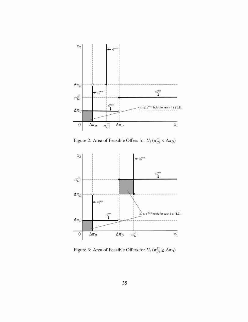
Figures 2 and 3 summarize the set of each manufacturer’s feasible offer (x1, x2) which sat-

isfies xi ∈ [0, xmax] for each i ∈ {1, 2}. Each manufacturer’s offer is feasible at the shadowed

area of Figures 2 and 3, which can be a candidate for the set of exclusion offers in the exclu-

sion equilibrium (x∗∗1 , x∗∗2 ); in other words, other area cannot be the exclusion equilibrium.

Depending on the magnitude relationship between πEiUi and ∆πD, we have two cases. First,

if πEiUi < ∆πD, summarized in Figure 2, each manufacturer’s exclusive offer is feasible at only

one region because D’s rejection profit is considerably high and each manufacturer cannot

11

compensate D profitably when its rival’s makes the higher offer. Second, if πEiUi ≥ ∆πD, sum-

marized in Figure 3, each manufacturer’s exclusive offer is feasible at two regions. Because

D’s rejection profit is not too high in this case, Ui can profitably offer xi(≥ ∆πD) when U j

makes the high offer x j ≥ (∆πD).

[Figures 2 and 3 about here]

To explore the existence of an exclusion equilibrium, we now combine the results in

Figures 1, 2, and 3. Figures 4 and 5 combine these figures and D’s decision at the shadowed

areas in Figures 2 and 3. Figures 4 implies that exclusion never occurs if πEiUi < ∆πD. In this

case, there exist only non-exclusion equilibria in which each manufacturer offers xi ∈ [0,∆πD)

and D rejects both offers. By contrast, Figure 5 shows that an exclusion equilibrium exists if

πEiUi ≥ ∆πD. The candidate for the equilibrium offer is the area in which (x1, x2) ∈ [∆πD, π

EiUi

]2

holds. Obviously, xi > x j ≥ ∆πD and xi = x j < πEiUi

cannot be an equilibrium because at least

one of the manufacturers has an incentive to deviate. There exists the exclusion equilibrium

in which each manufacturer offers x∗∗i = πEiUi and D accepts one of the offers. Note that even

when πEiUi ≥ ∆πD, there also exists the non-exclusion equilibria in which each manufacturer

offers xi ∈ [0,∆πD) and D rejects both offers.

[Figures 4 and 5 about here]

We finally consider the existence of an exclusion equilibrium. From the above discussion,

we need to check whether πEiUi ≥ ∆πD holds. By substituting equations (2) and (3), we obtain

πEiUi − ∆πD = (1 − 2β)(2Πd − Πm) ≥ 0,

if and only if β ∈ (0, 1/2]; which implies that an exclusion equilibrium exists for weak

bargaining power of D:

Proposition 2. Suppose that both manufacturers make exclusive offers in Stage 1 and adopt

two-part tariffs in Stage 2. If D has strong bargaining power (β > 1/2), exclusion cannot be

an equilibrium outcome. By contrast, if D has weak bargaining power (β ≤ 1/2), there exist

both an exclusion equilibrium and non-exclusion equilibria.

12

Proposition 2 shows that under the exclusive-offer competition, an exclusion equilibrium

exists depending on the bargaining power of D over manufacturers. For weak bargaining

power of D, D earns a smaller profit when it rejects both exclusive offers in Stage 1. There-

fore, each manufacturer can compensate D profitably. Moreover, the existence of exclusion

equilibrium does not depend on the degree of product substitution γ under non-linear whole-

sale pricing. Note that the result here highly depends on the assumption that manufacturers’

costs are symmetric. In the following subsection, we explore the case of an asymmetric cost

structure and we show that the exclusion equilibrium is more likely to be observed for lower

γ.

Note that Proposition 2 shows that exclusion is not a unique equilibrium outcome. By

comparing the two types of equilibria, the manufacturers strictly prefer the non-exclusion

equilibria to the exclusion equilibrium. Therefore, they do not have an incentive to yield

the exclusion outcome. By contrast, D has such an incentive. Because condition (4) holds

with strict inequality under the exclusion equilibrium, D prefers the exclusion equilibrium

to the non-exclusion equilibrium. Hence, D may try to do something to yield the exclusion

outcome.

3.4 Cost asymmetry

This subsection briefly discusses the effect of cost asymmetry on the existence of exclusion

equilibrium. Thus far, we assumed that each manufacturer operates at the same marginal cost

c ≥ 0. We now extend the model to the case in which manufacturers operate at different

marginal costs. Without loss of generality, we assume that the marginal cost of U1 is lower

than that of U2; namely, 0 ≤ c1 < c2. We define pmi and pdi as follows.

pmi ≡ arg maxpi

(pi − ci)Q(pi),

(pdi, pd j) ≡ arg maxpi,p j

(pi − ci)Q(pi, p j) + (p j − c j)Q(p j, pi.)

13

We define Πmi and Πdi be the net profit of Ui’s vertical chain under monopoly and under

duopoly;

Πmi ≡ (pmi − ci)Q(pmi), Πdi ≡ (pdi − ci)Q(pdi, pd j).

For the sake of notational convenience, we define ∆Πi ≡ Πdi + Πd j − Πm j, which can be

interpreted as the level of the industry profit increase when Ui’s product is also launched in

the market monopolized by U j. As in Assumption 1, we assume the following relationships:

Assumption 2. Πmi and Πdi have the following properties;

1. U1 earns higher profits than U2;

Πm1 > Πm2, Πd1 > Πd2. (8)

2. For each i ∈ {1, 2} and γ ∈ (0, 1),

Πd1 + Πd2 > Πmi > Πdi, (9)

where ∂Πmi/∂γ = 0, ∂Πdi/∂γ < 0, Πdi → Πmi as γ → 0, and Πd2 → 0 and Πd1 → Πm1

for sufficiently high γ.

3. ∆Π1 is decreasing in c1 but ∆Π2 is increasing in c1;

∂∆Π1

∂c1< 0,

∂∆Π2

∂c1> 0. (10)

Note that conditions (8) and (9) imply that we have ∆Π1 > ∆Π2 > 0, where the upstream

market becomes duopoly in the absence of exclusive dealing.

As in Section 3.1, the wholesale price between the negotiation between D and Ui is ci.

By using above definitions, the firms’ equilibrium profits under exclusive dealing, excluding

the fixed compensation xi, are

πEiUi = (1 − β)Πmi, π

EiU j = 0, πEi

D = βΠmi. (11)

14

By contrast, the firms’ equilibrium profits under non-exclusive dealing are

πRUi = (1 − β)∆Πi, π

RD = (1 − β)(Πmi − Πdi + Πm j − Πd j) + β(Πdi + Πd j). (12)

From condition (10), we have ∂πRU1/∂c1 < 0 but ∂πR

U2/∂c1 > 0, which is observed in the linear

demand model.15

We now consider the existence of exclusion equilibrium. We first explore the case in

which only Ui can make an exclusive offer. Substituting equations (11) and (12), we have

πEiUi + πEi

D − (πRUi + πR

D) = −β∆Π j < 0,

under condition (9), which implies that exclusion never occurs:

Proposition 3. Suppose both manufacturers adopt two-part tariffs. If U j is a potential entrant

and only Ui can makes an exclusive offer, Ui cannot exclude U j through exclusive contracts

even under asymmetric costs.

Proposition 3 implies that U1 cannot deter entry of U2 as long as entry increases the in-

dustry profit. Therefore, the result confirms the robustness of Chicago School argument in

the case where the incumbent manufacturer cannot deter entry of a potential entrant manu-

facturer, which is even less efficient.

We next consider the case in which both manufacturers make exclusive offers. Note that

the exclusion equilibrium exists if and only if πEiUi + πEi

D ≥ πRD holds for each i ∈ {1, 2}.

Substituting equations (11) and (12), we have πEiUi + πEi

D − πRD ≥ 0 if and only if

β ≤ βi ≡∆Πi

∆Πi + ∆Π j. (13)

for each i ∈ {1, 2}. From conditions (8), (9), and (13), βi have the following relationships;

0 < β2 <12< β1 < 1, (14)

where β1 → 1 and β2 → 0 as ∆Π2 → 0. Condition (14) shows that β1 > β2 always holds;

thus, the exclusion equilibrium exists if and only if β ≤ β2. Because β2 < 1/2 always15See Appendix C, which introduces the results under the linear demand model.

15

holds, cost asymmetry reduces the possibility of exclusion equilibrium. More precisely, by

differentiating βi with respect to c1, we have

∂βi

∂c1=

1(∆Πi + ∆Π j)2

(∂∆Πi

∂c1∆Π j −

∂∆Π j

∂c1∆Πi

).

Under condition (10), we have ∂β1/∂c1 < 0 and ∂β2/∂c1 > 0. Therefore, as U1 becomes more

efficient, β2 decreases; namely, the exclusion equilibrium is less likely to exist. The following

proposition summarizes the results provided above.

Proposition 4. Suppose that both manufacturers make exclusive offers in Stage 1 and adopt

two-part tariffs in Stage 2. As the degree of cost asymmetry increases, exclusion is less likely

to be an equilibrium outcome.

The result in Proposition 4 implies that the exclusion mechanism in this study is more

likely to work well when each manufacturer has the similar cost structure. When U1’s effi-

ciency increases, the industry profit under duopoly Πd1+Πd2 increases, which allows D to earn

higher profit under upstream duopoly because ∂πRD/∂c1 = −(1 − β)∂∆Π2/∂c1 + β(∂Πd1/∂c1 +

∂Πd2/∂c2) < 0. By contrast, the increase in U1’s efficiency does not affect U2’s monopoly

profit under exclusive dealing; namely, U2 has difficulty in compensating D. Therefore, the

possibility of exclusion becomes lower under cost asymmetry.

Finally, we explore the relationship between the existence of exclusion equilibrium and

the degree of product substitution γ. By differentiating βi with respect to γ, we have

∂βi

∂γ=

Πm j − Πmi

(∆Πi + ∆Π j)2

(∂Πdi

∂γ+∂Πd j

∂γ

)> 0 if and only if Πmi > Πm j.

From condition (8), we have ∂β1/∂γ > 0 and ∂β2/∂γ < 0, which leads to the following

proposition:

Proposition 5. Suppose that both manufacturers make exclusive offers in Stage 1 and adopt

two-part tariffs in Stage 2. Under cost asymmetry, the exclusion equilibrium is more likely to

be observed for the cases in which manufacturers produce highly differentiated products.

16

The result in Proposition 5 implies that under cost asymmetry, the existence of exclu-

sion equilibrium is determined by the degree of product substitution γ; that is, the result in

Proposition 2 highly depends on the symmetric cost structure. The result here is explained

by the property of bargaining when D rejects both exclusive offers. By differentiating πRD

with respect to γ, we have ∂πRD/∂γ = (2β − 1)(∂Πd1/∂γ + ∂Πd2/∂γ) > 0 for β < 1/2, which

implies that for weak bargaining power of D, its profits under upstream duopoly increases

with γ. Because U2 earns low monopoly profits under exclusive dealing, it has difficulty in

compensating D; thus, the exclusion equilibrium is less likely to be observed as the products

are less differentiated.

4 Linear wholesale pricing

This section explores the existence of anticompetitive exclusive dealing under linear whole-

sale pricing by assuming the standard linear demand with a representative consumer, in which

the demand for Ui’s product is provided by

Q(pi, p j) =

a − pi

bif 0 < pi ≤

−a(1 − γ) + p j

γ,

a(1 − γ) − pi + γp j

b(1 − γ2)if−a(1 − γ) + p j

γ< pi < a(1 − γ) + γp j,

0 if pi ≥ a(1 − γ) + γp j,

(15)

where i, j ∈ {1, 2} and i , j. Like the previous section, we assume that the industry profit

allocation after Stage 1 is given by Nash bargaining solution.

We first explore the case in which Ui’s exclusive offer is accepted in Stage 1. Under

exclusive dealing, the final consumer’s demand for Ui’s product becomes Q(pi) = (a− pi)/b.

We solve the game by using backward induction. In Stage 3, given wi determined in Stage 2,

D optimally chooses the price of Ui’s product; namely, p∗(wi) ≡ arg maxpi(pi − wi)Q(pi) =

(a + wi)/2. The optimal production level of Ui’s product supplied by D given wi becomes

Q∗(wi) ≡ Q(p∗(wi)) = (a−wi)/2b. In Stage 2, Ui and D negotiate and make a contract for the

linear wholesale price wEii . By defining D’s profit given wi as Π∗(wi) ≡ (p∗(wi)−wi)Q∗(wi), the

17

bargaining problem between D and Ui is described by the payoff pairs (Π∗(wi), (wi−c)Q∗(wi))

and the disagreement point (0, 0). The solution is given by:

wEii = arg max

wiβ log Π∗(wi) + (1 − β) log[(wi − c)Q∗(wi)].

The maximization problem leads to

wEii =

a + c − β(a − c)2

.

The firms’ equilibrium profits, excluding the fixed compensation xi, are

πEiUi =

(1 − β2)(a − c)2

8b, πEi

U j = 0, πEiD =

(1 + β)2(a − c)2

16b. (16)

We next explore the case in which D rejects both exclusive offers in Stage 1. In Stage 3,

given wholesale prices wi and w j determined in Stage 2, D optimally chooses the prices of

each manufacturer’s product (p∗(wi,w j), p∗(w j,wi)), where

(p∗(wi,w j), p∗(w j,wi)) ≡ arg maxpi,p j

(pi − wi)Q(pi, p j) + (p j − w j)Q(p j, pi),

where i, j ∈ {1, 2} and i , j. The production level of each final product supplied by D given

wi and w j is given by

Q∗(wi,w j) ≡ Q(p∗(wi,w j), p∗(w j,wi)) =a − wi − γ(a − w j)

2(1 − γ2)b,

In Stage 2, U1, U2, and D makes contract(s) for the linear wholesale prices, wR1 and wR

2 .

By defining D’s profit from selling Ui’s product given (wi,w j) as Π∗(wi,w j) ≡ (p∗(wi,w j) −

wi)Q∗(wi,w j), the bargaining problem between D and Ui is described by the payoff pairs

(Π∗(wRi ,w

Rj ) + Π∗(wR

j ,wRi ), (wR

i − c)Q∗(wRi ,w

Rj )) and the disagreement point (Π∗(wR

j ), 0), where

Π∗(wRj ) is D’s profit when it sells only U j’s product given the linear wholesale price wR

j . The

solution is given by:

wRi = arg max

wiβ log[Π∗(wi,w j) + Π∗(w j,wi) − Π∗(w j)] + (1 − β) log[(wi − c)Q∗(wi,w j)].

18

The maximization problem leads to

wRi =

a(1 − γ) + c − β(a(1 − γ) − c)2 − γ(1 − β)

,

for each i ∈ {1, 2}. The resulting profits of firms are given as

πRUi =

(1 − β2)(1 − γ)(a − c)2

2b(1 + γ)(2 − γ(1 − β))2 , πRD =

(1 + β)2(a − c)2

2b(1 + γ)(2 − γ(1 − β))2 . (17)

We now explore the existence of exclusion. Like the case of two-part tariffs, when only

Ui can make an exclusive offer, exclusion never occurs:

Proposition 6. Suppose both manufacturers offer linear wholesale prices. If U j is a potential

entrant and only Ui can makes an exclusive offer, Ui cannot exclude U j through exclusive

contracts for any pair of bargaining power allocation and the degree of product substitution.

Proof. See Appendix A.1. �

Proposition 6 implies that in the absence of exclusive-offer competition, anticompetitive

exclusive dealing cannot occur, which can be explained by the logic underlying the Chicago

School argument. When D accepts the exclusive offer from Ui in Stage 1.1, Ui can enjoy

monopoly profits. However, Ui cannot maximize the joint profit between Ui and D under

linear wholesale pricing due to the double marginalization problem. On the contrary, when D

rejects Ui’s exclusive offer in Stage 1.1, U j enters the upstream market in Stage 1.2. Because

of upstream competition, Ui ’s wholesale price decreases and D can earn considerably higher

rejection profits; namely, profit loss under exclusive dealing ∆πD is significantly large. In

addition, a higher degree of product substitution allows Ui to earn a higher profit even in

the case of entry, which reduces Ui’s profit increase through exclusion, ∆πU . Therefore, like

the Chicago School argument, Ui cannot profitably compensate D; anticompetitive exclusive

dealing cannot occur.

By contrast, when both manufacturers can make exclusive offers, an exclusion equilib-

rium exists under some conditions:

19

Proposition 7. Suppose that both manufacturers make exclusive offers in Stage 1 and linear

wholesale prices are determined through Nash bargaining in Stage 2. When the products

are less differentiated (γ > γ ' 0.77393), exclusion cannot be an equilibrium outcome. By

contrast, when those are sufficiently differentiated (γ ≤ γ), there exist both an exclusion

equilibrium and non-exclusion equilibria for sufficiently weak bargaining power of D (β ≤

β(γ)), where

β(γ) ≡4φ2 + 2γ(1 + γ)(5γ − 4)φ + 4γ2(1 + γ)(γ3 + 3γ2 + 3γ − 5)

6γ2(1 + γ)φ,

and

φ ≡[γ3(1 + γ)2(γ4 + 4γ3 + 6γ2 − 32γ + 19)

+3√

6γ6(1 + γ)2(1 − γ2)(γ5 + 5γ4 + 10γ3 + 5γ3 − 12γ2 − 11γ + 9

)] 13

.

Proof. See Appendix A.2. �

Note that β(γ) has a single peaked property with β(γ) → 1/3 as γ → 0, β(γ) → 0 as γ → γ,

and the maximized value β(γ∗) ' 0.413049 at γ∗ ' 0.469146.

[Figure 6 about here]

Figure 6 summarizes Proposition 7. The notable result in Proposition 7 is that linear

wholesale pricing leads to the low possibility of the anticompetitive exclusion equilibrium

when the exclusive-offer competition occurs; exclusion never occurs for less differentiated

manufacturers’ products. Note that the major difference between two types of pricing is the

existence of a double marginalization problem, which becomes serious for weak bargaining

power of D. The double marginalization problem occurs not only under exclusive dealing

but also under the case where D deals with both manufacturers. More importantly, when D

deals with both manufacturers, the seriousness of double marginalization problem depends

on the degree of production substitution γ. When the manufacturers produce almost homo-

geneous products, the double marginalization problem is not too serious, which allows D

20

to earn large rejection profits πRD. Hence, the exclusion equilibrium does not exist when the

products are less differentiated. By contrast, as those are differentiated, the double marginal-

ization problem becomes serious; namely, the rent extraction by each manufacture becomes

significant. This prevents D from earning large rejection profits while the industry profit in-

creases. Therefore, the manufacturers can compensate D profitably if those are sufficiently

differentiated.

Figure 6 also shows that β(γ) has the single peaked property, which implies that the pos-

sibility of the exclusion equilibrium is non-monotonic in the degree of product substitution

γ. Because only D’s rejection profit πRD depends on γ in πEi

Ui − ∆πD, this phenomenon can be

explained by the following two effects on πRD. First, as the products are differentiated, the dou-

ble marginalization problem when D deals with both manufacturers becomes serious, which

is pointed out above. This becomes more serious as β is smaller, which enables the manu-

facturers to set higher wi. Second, as those are differentiated, the industry profit increases.

This would allow D to earn higher rejection profits if the wholesale prices were exogenously

fixed. This positive effect is weaker as β is smaller because D’s profit share is small. The

magnitude of these two effects is determined by the degree of product substitution and that

of D’s bargaining power. By differentiating πRD with respect to γ, we obtain the following

relationship;

∂πRD

∂γ=

(1 + β)2(3γ − β(2 + 3γ))b(1 + γ)2(2 − γ(1 − β))3 < 0, if and only if β > β(γ) ≡

3γ2 + 3γ

or γ <2β

3(1 − β).

The properties of β(γ) are summarized in Figure 6. This relationship implies that when

β ≤ 1/2, as manufacturers become differentiated when they produce almost homogeneous

products, D’s rejection profit decreases for all because the double marginalization problem

when D deals with both manufacturers is more serious. By contrast, as manufacturers become

differentiated when they produce sufficiently differentiated products, D’s rejection profit is

more likely to increase for sufficiently strong D’s bargaining power because the increase in

the industry profit is the dominant effect.

21

5 Conclusion

This study has explored the existence of anticompetitive exclusive dealing when all upstream

firms can make exclusive offers. Most of previous studies consider anticompetitive exclusive

dealing to deter a potential entrant, which cannot make an exclusive offer. However, in real-

world situation, existing firms are often excluded. Therefore, we need to consider how the

existence of exclusive-offer competition affects the possibility of exclusion to apply the model

to these cases.

We show that a seemingly small difference in the setting turns out to be crucial. In contrast

to the case where one of the upstream firms is a potential entrant, the existence of exclusive-

offer competition eliminates the upstream firms’ outside option to earn positive profits when

it fails to exclude the rival upstream firm. We point out that this induces upstream firms to

make higher exclusive offers and show that when the downstream firm has weak bargaining

power, anticompetitive exclusive dealing can be an equilibrium outcome in the two-part tariff

setting of general demand function and Nash bargaining. Moreover, this result hold in various

setting; the exclusion outcome identified in this study can be widely applied to diverse real-

world vertical relationships.

The finding here provides new implication for antitrust agencies; anticompetitive exclu-

sive dealing is more likely to be observed when upstream firms are existing firms. In addition,

because the downstream firm has an strong incentive to engage in anticompetitive exclusive

dealing, the downstream firm is more likely to lead the negotiation of anticompetitive exclu-

sive dealing when upstream firms are existing firms.

Several outstanding issues require future research. First, there is a concern about up-

stream firms’ behavior needed to achieve market environment where exclusive dealing is

impossible. Although we assume that the level of product substitution or bargaining power

are exogenously given parameters, upstream firms could control these parameters. Second,

there is a concern about this study’s relationship with other studies on anticompetitive ex-

clusive dealing. We predict that if we add the exclusive-offer competition into the previous

22

studies, exclusion becomes less costly. We hope that this study will assist future researchers

in addressing these issues.

23

A Proofs of Results

A.1 Proof of Proposition 6

We show that condition (6) never holds; that is, by substituting equations (16) and (17), we

have

∆πU − ∆πD = −(a − c)2(1 + β)(8 − (1 + γ)(2 − γ(1 − β))(3 − β))

16b(1 + γ)(2 − γ(1 − β))< 0, (18)

for all (β, γ) ∈ (0, 1)2. Let η(β, γ) ≡ −8 + (1 + γ)(2 − γ(1 − β))(3 − β). Note that η(β, γ) < 0 if

and only if condition (18) holds. By differentiating η(β, γ) with respect to β and γ, we have

ηβ(β, γ) R 0⇔ β Q K(γ) ≡−1 + 2γ

γ,

ηγ(β, γ) R 0⇔ β R L(γ) ≡−1 + 2γ1 + 2γ

.

Note that for γ ∈ (1/2, 1], K′(γ) > L′(γ) > 0 and K(γ) > L(γ) > 0 and that K(1/2) =

L(1/2) = 0 and K(1) = 1 and L(1) = 1/3. Figure 7 summarizes the properties of ηβ(β, γ)

and ηγ(β, γ). There are six regions in (β, γ) ∈ [0, 1]2 such that (i) ηβ(β, γ) = ηγ(β, γ) = 0, (ii)

ηβ(β, γ) < 0, ηγ(β, γ) > 0, (iii) ηβ(β, γ) = 0, ηγ(β, γ) > 0 , (iv) ηβ(β, γ) > 0, ηγ(β, γ) > 0, (v)

ηβ(β, γ) > 0, ηγ(β, γ) = 0, and (vi) ηβ(β, γ) > 0, ηγ(β, γ) < 0. Arrows in Figure 7 indicate the

direction of an increase in η(β, γ) for each region. From Figure 7, for (β, γ) = (0, 1/2), η(β, γ)

takes the locally maximized value in region (i), where we have η(β, γ) = −5/4 < 0. More

importantly, Figure 7 shows that η(β, γ) is globally maximized in the domain (β, γ) ∈ [0, 1]2

when (β, γ) = (1, 1) where we have η(1, 1) = 0. Therefore, η(β, γ) < 0 for all (β, γ) ∈ (0, 1)2.

Q.E.D.

A.2 Proof of Proposition 7

We check whether πEiUi≥ ∆πD holds. By substituting equations (16) and (17), we obtain

πEiUi − ∆πD ≥ 0 if and only if γ ≤ γ and β ≤ β(γ) < 1/2.

Q.E.D.

24

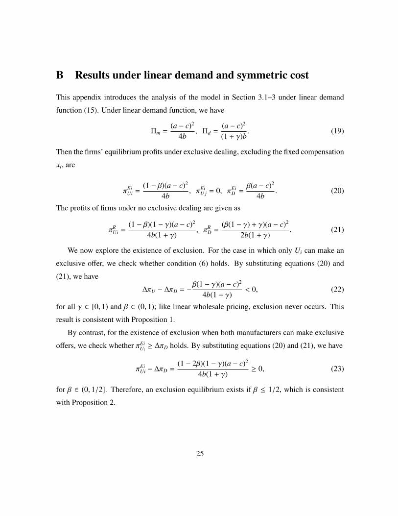
B Results under linear demand and symmetric cost

This appendix introduces the analysis of the model in Section 3.1–3 under linear demand

function (15). Under linear demand function, we have

Πm =(a − c)2

4b, Πd =

(a − c)2

(1 + γ)b. (19)

Then the firms’ equilibrium profits under exclusive dealing, excluding the fixed compensation

xi, are

πEiUi =

(1 − β)(a − c)2

4b, πEi

U j = 0, πEiD =

β(a − c)2

4b. (20)

The profits of firms under no exclusive dealing are given as

πRUi =

(1 − β)(1 − γ)(a − c)2

4b(1 + γ), πR

D =(β(1 − γ) + γ)(a − c)2

2b(1 + γ). (21)

We now explore the existence of exclusion. For the case in which only Ui can make an

exclusive offer, we check whether condition (6) holds. By substituting equations (20) and

(21), we have

∆πU − ∆πD = −β(1 − γ)(a − c)2

4b(1 + γ)< 0, (22)

for all γ ∈ [0, 1) and β ∈ (0, 1); like linear wholesale pricing, exclusion never occurs. This

result is consistent with Proposition 1.

By contrast, for the existence of exclusion when both manufacturers can make exclusive

offers, we check whether πEiUi≥ ∆πD holds. By substituting equations (20) and (21), we have

πEiUi − ∆πD =

(1 − 2β)(1 − γ)(a − c)2

4b(1 + γ)≥ 0, (23)

for β ∈ (0, 1/2]. Therefore, an exclusion equilibrium exists if β ≤ 1/2, which is consistent

with Proposition 2.

25

C Results under linear demand and asymmetric cost

This appendix introduces the analysis of the model in Section 3.4 under linear demand

function (15). We measure U1’s cost advantage by θ, where c2 = θpm1 + (1 − θ)c1 and

pm1 = (a + c1)/2. θ = 0 implies that U1 has no cost advantage. As θ increases, U1 becomes

efficient. We assume the following relationship;

0 < θ < min{2(1 − γ), 1}. (24)

If condition (24) holds, the upstream market becomes duopoly if the exclusive offer is re-

jected. When D accepts U1’s exclusive offer, the firms’ equilibrium profits, excluding the

fixed compensation x1, are

πE1U1 =

(1 − β)(a − c2)2

(2 − θ)2b, πE1

U2 = 0, πE1D =

β(a − c2)2

(2 − θ)2b. (25)

Likewise, when D accepts U2’s exclusive offer, the firms’ equilibrium profits, excluding the

fixed compensation x2, are

πE2U2 =

(1 − β)(a − c2)2

4b, πE2

U1 = 0, πE2D =

β(a − c2)2

4b. (26)

By contrast, when D rejects both exclusive offers, the firms’ equilibrium profits are

πRD =

(θ2 + 4(1 − γ)(2 − θ) − (1 − β)((2(1 − γ) + θγ)2 + (2(1 − γ) − θ)2))(a − c2)2

4b(1 − γ2)(2 − θ)2 ,

πRU1 =

(1 − β)(2(1 − γ) + θγ)2(a − c2)2

4b(1 − γ2)(2 − θ)2 , πRU2 =

(1 − β)(2(1 − γ) + θ)2(a − c2)2

4b(1 − γ2)(2 − θ)2 .

(27)

We now consider the existence of an exclusion equilibrium when both manufacturers

make exclusive offers. By substituting (25), (26) and (27), πEiUi + πEi

D − πRD ≥ 0 if and only if

β ≤ βi(γ, θ), where

β1(γ, θ) ≡(2(1 − γ) + θγ)2

4(1 − γ)2(2 − θ) + θ2(1 + γ2), β2(γ, θ) ≡

(2(1 − γ) − θ)2

4(1 − γ)2(2 − θ) + θ2(1 + γ2).

The following lemma summarizes the properties of βi(γ, θ);

26

Proposition C.1. βi(γ, θ) has the following properties;

1. 0 < β2 < 1/2 < β1 < 1.

2. ∂β1/∂γ > 0 and ∂β2/∂γ < 0.

3. ∂β1/∂θ > 0 and ∂β2/∂θ < 0.

4. As γ → (2 − θ)/2, β1 → 1 and β2 → 0.

5. As θ → 0, β1 → 1/2 and β2 → 1/2.

Proof. We first examine the first property. Note that β2 > 0 is obvious. Then, we have

β1 −12

=12− β2 =

(θ(4 − θ)(1 − γ))2

2(4(1 − γ)2(2 − θ) + θ2(1 + γ2))> 0,

1 − β1 =(2(1 − γ) − θ)2

4(1 − γ)2(2 − θ) + θ2(1 + γ2)> 0.

Therefore, the first property holds. The second and third properties can be derived by the

following results; under condition (24)

∂β1

∂γ=

2θ(4 − θ)(2(1 − γ) + θγ)(2(1 − γ) − θ)4(1 − γ)2(2 − θ) + θ2(1 + γ2)

> 0,

∂β2

∂γ= −

2θ(4 − θ)(2(1 − γ) + θγ)(2(1 − γ) − θ)4(1 − γ)2(2 − θ) + θ2(1 + γ2)

< 0,

∂β1

∂θ=

4(1 − γ2)(2(1 − γ) + θγ)(2(1 − γ) − θ)4(1 − γ)2(2 − θ) + θ2(1 + γ2)

> 0,

∂β2

∂γ= −

4(1 − γ2)(2(1 − γ) + θγ)(2(1 − γ) − θ)4(1 − γ)2(2 − θ) + θ2(1 + γ2)

< 0.

The fourth and fifth properties are obtained by substituting γ = (2 − θ)/2 and θ = 0 into

βi(γ, θ), which is continuous in θ and γ.

�

27

D Exclusive supply contracts when downstream firms com-pete in quantity

This appendix introduces another case where exclusive-offer competition plays an essential

role in exclusive dealing. The upstream market is composed of an upstream monopolist U,

whose marginal cost is c ≥ 0. The downstream market is composed of two downstream

firms which produce homogeneous products. Each downstream firm produces one unit of

final product by using one unit of input produced by U. For simplicity, we assume that the

cost of transformation is zero for each Di; given the input price w, per unit production cost

of Di is given by cDi = wi, where i ∈ {1, 2}. D1 and D2 compete in quantity. Let Qi be the

production level of Di. We assume that the inverse demand for the final product P(Q) is given

by a simple linear function:

P(Q) = a − bQ,

where Q ≡ Q1 + Q2 is the output of the final product, a > c, and b > 0.

The model in this appendix contains three stages. In Stage 1, D1 and D2 make exclusive

supply offers to U with fixed compensation yi ≥ 0, where i ∈ {1, 2}. U can reject both offers or

it can accept one of the offers. As defined in Section 2, let ω ∈ {R, E1, E2} be U’s decision in

Stage 1. If U is indifferent between two exclusive offers and the acceptance is more profitable,

it accepts one of the offers with probability 1/2. In Stage 2, U offers a linear wholesale price

w to active downstream firms. The equilibrium wholesale price offered by U is denoted by

wω. In Stage 3, active downstream firms order input and determine the production level of

the final product Qi. Di’s profit is denoted by πωDi. Likewise, U’s profit is denoted by πωU .

D.1 Equilibrium outcomes after Stage 1

We first explore the case in which Di’s exclusive supply offer is accepted by U in Stage 1.

In Stage 3, given w, Di optimally chooses the production level QEii (w) ≡ arg maxQi(P(Qi) −

w)Qi = (a − w)/2b. Then the input demand for U becomes QEi(w) = QEii (w) = (a − w)/2b.

In Stage 2, by anticipating these results, U optimally choose input price wEi ≡ arg maxw(w −

28

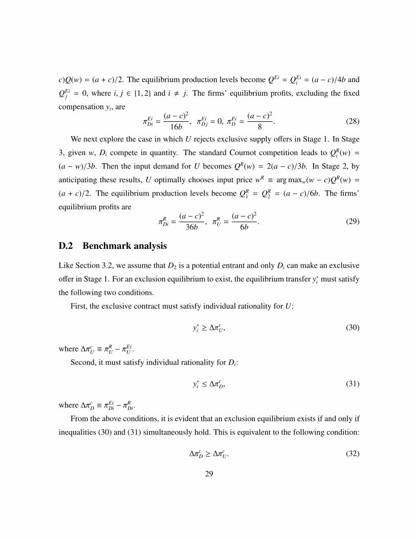
c)Q(w) = (a + c)/2. The equilibrium production levels become QEi = QEii = (a − c)/4b and

QEij = 0, where i, j ∈ {1, 2} and i , j. The firms’ equilibrium profits, excluding the fixed

compensation yi, are

πEiDi =

(a − c)2

16b, πEi

D j = 0, πEiD =

(a − c)2

8. (28)

We next explore the case in which U rejects exclusive supply offers in Stage 1. In Stage

3, given w, Di compete in quantity. The standard Cournot competition leads to QRi (w) =

(a − w)/3b. Then the input demand for U becomes QR(w) = 2(a − c)/3b. In Stage 2, by

anticipating these results, U optimally chooses input price wR ≡ arg maxw(w − c)QR(w) =

(a + c)/2. The equilibrium production levels become QR1 = QR

2 = (a − c)/6b. The firms’

equilibrium profits are

πRDi =

(a − c)2

36b, πR

U =(a − c)2

6b. (29)

D.2 Benchmark analysis

Like Section 3.2, we assume that D2 is a potential entrant and only Di can make an exclusive

offer in Stage 1. For an exclusion equilibrium to exist, the equilibrium transfer y∗i must satisfy

the following two conditions.

First, the exclusive contract must satisfy individual rationality for U:

y∗i ≥ ∆πcU , (30)

where ∆πcU ≡ π

RU − π

EiU .

Second, it must satisfy individual rationality for Di:

y∗i ≤ ∆πcD, (31)

where ∆πcD ≡ π

EiDi − π

RDi.

From the above conditions, it is evident that an exclusion equilibrium exists if and only if

inequalities (30) and (31) simultaneously hold. This is equivalent to the following condition:

∆πcD ≥ ∆πc

U . (32)

29

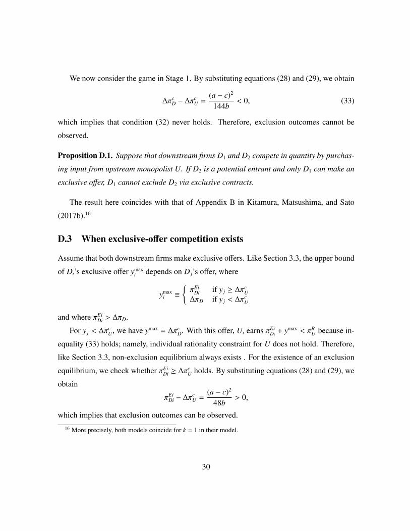
We now consider the game in Stage 1. By substituting equations (28) and (29), we obtain

∆πcD − ∆πc

U =(a − c)2

144b< 0, (33)

which implies that condition (32) never holds. Therefore, exclusion outcomes cannot be

observed.

Proposition D.1. Suppose that downstream firms D1 and D2 compete in quantity by purchas-

ing input from upstream monopolist U. If D2 is a potential entrant and only D1 can make an

exclusive offer, D1 cannot exclude D2 via exclusive contracts.

The result here coincides with that of Appendix B in Kitamura, Matsushima, and Sato

(2017b).16

D.3 When exclusive-offer competition exists

Assume that both downstream firms make exclusive offers. Like Section 3.3, the upper bound

of Di’s exclusive offer ymaxi depends on D j’s offer, where

ymaxi ≡

{πEi

Di if y j ≥ ∆πcU

∆πD if y j < ∆πcU

and where πEiDi > ∆πD.

For y j < ∆πcU , we have ymax = ∆πc

D. With this offer, Ui earns πEiDi

+ ymax < πRU because in-

equality (33) holds; namely, individual rationality constraint for U does not hold. Therefore,

like Section 3.3, non-exclusion equilibrium always exists . For the existence of an exclusion

equilibrium, we check whether πEiDi ≥ ∆πc

U holds. By substituting equations (28) and (29), we

obtain

πEiDi − ∆πc

U =(a − c)2

48b> 0,

which implies that exclusion outcomes can be observed.

16 More precisely, both models coincide for k = 1 in their model.

30

Proposition D.2. Suppose that downstream firms D1 and D2 compete in quantity by purchas-

ing input from upstream monopolist U. When both downstream firms can make exclusive

offers, there exist both an exclusion equilibrium and a non-exclusion equilibrium. In the

exclusion equilibrium, both D1 and D2 offer y∗i = πEiDi> ∆πU and U earns all industry profits.

References

Abito, J.M., and Wright, J., 2008. Exclusive Dealing with Imperfect Downstream Competi-

tion. International Journal of Industrial Organization 26(1), 227–246.

Aghion, P., and Bolton, P., 1987. Contracts as a Barrier to Entry. American Economic Re-

view 77(3), 388–401.

Argenton, C., 2010. Exclusive Quality. Journal of Industrial Economics 58(3), 690–716.

Bernheim, B.D., and Whinston, M.D., 1998. Exclusive Dealing. Journal of Political Econ-

omy 106(1), 64–103.

Bork, R.H., 1978. The Antitrust Paradox: A Policy at War with Itself. New York: Basic

Books.

Calzolari, G., and Denicolo, V., 2013. Competition with Exclusive Contracts and Market-Share

Discounts. American Economic Review 103(6), 2384–2411.

Calzolari, G., and Denicolo, V., 2015. Exclusive Contracts and Market Dominance. Ameri-

can Economic Review 105(11), 3321–3351.

Choi, J.P., and Stefanadis, C., forthcoming. Sequential Innovation, Naked Exclusion, and Up-

front Lump-sum Payments. Economic Theory.

DeGraba, P., 2013. Naked Exclusion by an Input Supplier: Exclusive Contracting Loyalty

Discounts. International Journal of Industrial Organization 31(5), 516–526.

31

Farrell, J., 2005. Deconstructing Chicago on Exclusive Dealing. Antitrust Bulletin 50, 465–

80.

Fumagalli, C., and Motta, M., 2006. Exclusive Dealing and Entry, When Buyers Compete.

American Economic Review 96(3), 785–795.

Fumagalli, C., Motta, M., and Persson, L., 2009. On the Anticompetitive Effect of Exclusive

Dealing When Entry by Merger Is Possible. Journal of Industrial Economics 57(4),

785–811.

Fumagalli, C., Motta, M., and Rønde, T., 2012. Exclusive Dealing: Investment Promotion may

Facilitate Inefficient Foreclosure. Journal of Industrial Economics 60(4), 599–608.

Gratz, L. and Reisinger, M., 2013. On the Competition Enhancing Effects of Exclusive Deal-

ing Contracts. International Journal of Industrial Organization 31(5), 429-437.

Kitamura, H., 2010. Exclusionary Vertical Contracts with Multiple Entrants. International

Journal of Industrial Organization 28(3), 213–219.

Kitamura, H., Matsushima, N., and Sato, M., 2016. Exclusive Contracts with Complemen-

tary Input. mimeo.

http://ssrn.com/abstract=2547416

Kitamura, H., Matsushima, N., and Sato, M., 2017a. Exclusive Contracts and Bargaining Power.

Economics Letters 151, 1–3.

Kitamura, H., Matsushima, N., and Sato, M., 2017b. How Does Downstream Firms’ Efficiency

Affect Exclusive Supply Agreements? mimeo.

http://ssrn.com/abstract=2306922

Motta, M., 2004. Competition Policy. Theory and Practice. Cambridge: Cambridge Univer-

sity Press.

32

Posner, R.A., 1976. Antitrust Law: An Economic Perspective. Chicago: University of Chicago

Press.

Rasmusen, E.B., Ramseyer, J.M., and Wiley Jr., J.S., 1991. Naked Exclusion. American Eco-

nomic Review 81(5), 1137–1145.

Segal, I.R., and Whinston, M.D., 2000. Naked Exclusion: Comment. American Economic

Review 90(1), 296–309.

Shen, B., 2014. Naked exclusion by a manufacturer without a first-mover advantage, mimeo.

Simpson, J., and Wickelgren, A.L., 2007. Naked Exclusion, Efficient Breach, and Downstream

Competition. American Economic Review 97(4), 1305–1320.

Whinston, M.D., 2006. Lectures on Antitrust Economics. Cambridge: MIT Press.

Wright, J., 2008. Naked Exclusion and the Anticompetitive Accommodation of Entry. Eco-

nomics Letters 98(1), 107–112.

Wright, J., 2009. Exclusive Dealing and Entry, when Buyers Compete: Comment. American

Economic Review 99(3), 1070–1081.

Yong, J.S., 1996. Excluding Capacity-Constrained Entrants Through Exclusive Dealing: The-

ory and an Application to Ocean Shipping. Journal of Industrial Economics 44(2),

115–29.

Yong, J.S., 1999. Exclusionary Vertical Contracts and Product Market Competition. Journal

of Business 72(3), 385-406.

33

𝑥1

𝑥2

Δ𝜋𝐷

Δ𝜋𝐷0

𝐸1

𝐸2

𝑅

𝑥1 = 𝑥2 (𝐸𝑖 with probability 1/2)

𝐸1

(𝑥2 > Δ𝜋𝐷 > 𝑥1)

𝐸2(𝑥2 > 𝑥1 > Δ𝜋𝐷)

(𝑥1 > 𝑥2 > Δ𝜋𝐷)

(𝑥1 > Δ𝜋𝐷 > 𝑥2)

(Δ𝜋𝐷 > 𝑥2 > 𝑥1)

𝑅(Δ𝜋𝐷 > 𝑥1 > 𝑥2)

Figure 1: Individual Rationality for D

34

𝑥1

𝑥2

Δ𝜋𝐷

Δ𝜋𝐷0

Δ𝜋𝑈

Δ𝜋𝑈 𝜋𝑈𝑖𝐸𝑖

𝜋𝑈𝑖𝐸𝑖

𝑥1max

𝑥1max

𝑥2max

𝑥2max

𝑥𝑖 ≤ 𝑥max holds for each 𝑖 ∈ {1,2}.

Figure 2: Area of Feasible Offers for Ui (πEiUi < ∆πD)

𝑥1

𝑥2

Δ𝜋𝐷

Δ𝜋𝐷0

Δ𝜋𝑈

Δ𝜋𝑈 𝜋𝑈𝑖𝐸𝑖

𝜋𝑈𝑖𝐸𝑖

𝑥1max

𝑥1max

𝑥2max

𝑥2max 𝑥𝑖 ≤ 𝑥max holds for each 𝑖 ∈ {1,2}.

Figure 3: Area of Feasible Offers for Ui (πEiUi ≥ ∆πD)

35

𝑥1

𝑥2

Δ𝜋𝐷

Δ𝜋𝐷0

Δ𝜋𝑈

Δ𝜋𝑈 𝜋𝑈𝑖𝐸𝑖

𝜋𝑈𝑖𝐸𝑖

𝑥1max

𝑥1max

𝑥2max

𝑥2max

𝑅

Figure 4: Existence of An Exclusion Equilibrium for πEiUi < ∆πD

𝑥1

𝑥2

Δ𝜋𝐷

Δ𝜋𝐷0

Δ𝜋𝑈

Δ𝜋𝑈 𝜋𝑈𝑖𝐸𝑖

𝜋𝑈𝑖𝐸𝑖

𝑥1max

𝑥1max

𝑥2max

𝑥2max

Exclusion Equilibrium

𝑅

𝐸2

𝐸1

𝑥1 = 𝑥2 (𝐸𝑖 with probability 1/2)

Figure 5: Existence of An Exclusion Equilibrium for πEiUi ≥ ∆πD

36

𝛾

𝛽

𝑛𝑜𝐸𝐷

𝐸𝐷𝑖/𝑛𝑜𝐸𝐷 𝛽(𝛾)

𝛽(𝛾)

Figure 6: Existence of An Exclusion Equilibrium under Linear wholesale pricing

37

0.0 0.1 0.2 0.3 0.4 0.5 0.6 0.7 0.8 0.9 1.00.0

0.1

0.2

0.3

0.4

0.5

0.6

0.7

0.8

0.9

1.0

𝛽

𝛾

𝜂𝛽 < 0

𝜂𝛾 > 0

𝜂𝛽 = 0

𝜂𝛾 > 0 𝜂𝛽 > 0

𝜂𝛾 > 0

𝜂𝛽 > 0

𝜂𝛾 < 0

𝜂𝛽 > 0

𝜂𝛾 = 0

𝜂𝛽 = 𝜂𝛾 = 0

𝐾(𝛾)

𝐿(𝛾)

Figure 7: Properties of ηβ(β, γ) and ηγ(β, γ)

38