MorningstarAdvisor.com 25

tails. Well-known examples are Benoit Mandelbrot’s Lévy stable hypothesis (Mandelbrot, 1963), the Student’s t-distribution (Blattberg and Gonedes, 1974), and the mixture-of-Gaussian distributions hypothesis (Clark, 1973). Each, however, has its drawbacks.

The latter two models possess fat tails and finite variance, but they lack scaling properties. In other words, the models do a good job of capturing the outliers and putting bookends around possible results, but the shapes of their distributions change at different time intervals.

A promising alternative is the Lévy stable distribution model (Lévy, 1925). In 1963, Mandelbrot modeled cotton prices with a Lévy stable process, and his finding was later supported by Eugene Fama in 1965. A Lévy stable distribution model has fat tails and obeys scaling properties, but it has an infinite variance—which greatly complicates things. How can an investor model a portfolio’s risk if it has infinite downside or upside returns? In a nutshell, the Lévy model’s tails are too fat.

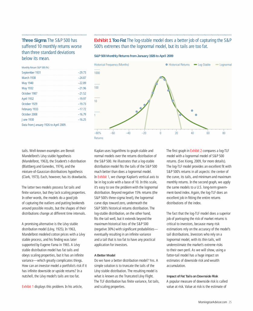
Exhibit 1 displays this problem. In his article,

Kaplan uses logarithms to graph stable and normal models over the returns distribution of the S&P 500. He illustrates that a log-stable distribution model fits the tails of the S&P 500 much better than does a lognormal model. In Exhibit 1, we change Kaplan’s vertical axis to be in log scale with a base of 10. In this scale, it’s easy to see the problem with the lognormal distribution. Beyond negative 15% returns (the S&P 500’s three-sigma level), the lognormal curve dips toward zero, underneath the S&P 500’s historical returns distribution. The log-stable distribution, on the other hand, fits the tail well, but it extends beyond the maximum historical loss of the S&P 500 (negative 30%) with significant probabilities—eventually resulting in an infinite variance and a tail that is too fat to have any practical application for investors.

A Better Model

Do we have a better distribution model? Yes. A simple solution is to truncate the tails of the Lévy stable distribution. The resulting model is what is known as the Truncated Lévy Flight. The TLF distribution has finite variance, fat tails, and scaling properties.

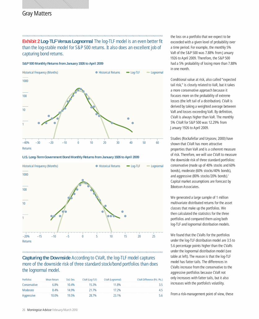
The first graph in Exhibit 2 compares a log-TLF model with a lognormal model of S&P 500 returns. (See Xiong, 2009, for more details). The log-TLF model provides an excellent fit with S&P 500’s returns in all aspects: the center of the curve, its tails, and minimum and maximum monthly returns. In the second graph, we apply the same models to a U.S. long-term govern-ment-bond index. Again, the log-TLF does an excellent job in fitting the entire returns distributions of the index.

The fact that the log-TLF model does a superior job of portraying the risk of market returns is critical to investors, because many risk estimations rely on the accuracy of the model’s tail distributions. Investors who rely on a lognormal model, with its thin tails, will underestimate the market’s extreme risks to their own peril. As we will show, using a fatter-tail model has a huge impact on estimates of downside risk and wealth accumulation.

Impact of Fat Tails on Downside Risk

A popular measure of downside risk is called value at risk. Value at risk is the estimate of

Exhibit 1 Too Fat The log-stable model does a better job of capturing the S&P 500’s extremes than the lognormal model, but its tails are too fat.

S&P 500 Monthly Returns from January 1926 to April 2009

1

10

100

1000

–80% –60 –40 –20 0 20 40 60 80

Log-Stable LognormalHistorical Frequency (Months)

Returns

Historical Returns

Three Sigma The S&P 500 hassuffered 10 monthly returns worse than three standard deviationsbelow its mean.

Monthly Return S&P 500 (%)

September 1931 –29.73

March 1938 –24.87

May 1940 –22.89

May 1932 –21.96

October 1987 –21.52

April 1932 –19.97

October 1929 –19.73

February 1933 –17.72

October 2008 –16.79

June 1930 –16.25

Data from January 1926 to April 2009.

Morningstar Advisor February/March 201026

Gray Matters

the loss on a portfolio that we expect to be exceeded with a given level of probability over a time period. For example, the monthly 5% VaR of the S&P 500 was 7.88% from January 1926 to April 2009. Therefore, the S&P 500 had a 5% probability of losing more than 7.88% in one month.

Conditional value at risk, also called “expected tail risk,” is closely related to VaR, but it takes a more conservative approach because it focuses more on the probability of extreme losses (the left tail of a distribution). CVaR is derived by taking a weighted average between VaR and losses exceeding VaR. By definition, CVaR is always higher than VaR. The monthly 5% CVaR for S&P 500 was 12.29% from January 1926 to April 2009.

Studies (Rockafellar and Uryasev, 2000) have shown that CVaR has more attractive properties than VaR and is a coherent measure of risk. Therefore, we will use CVaR to measure the downside risk of three standard portfolios: conservative (made up of 40% stocks and 60% bonds), moderate (60% stocks/40% bonds), and aggressive (80% stocks/20% bonds).1 Capital market assumptions are forecast by Ibbotson Associates.

We generated a large sample of 1 million multivariate distributed returns for the asset classes that make up the portfolios. We then calculated the statistics for the three portfolios and compared them using both log-TLF and lognormal distribution models.

We found that the CVaRs for the portfolios under the log-TLF distribution model are 3.5 to 5.6 percentage points higher than the CVaRs under the lognormal distribution model (see table at left). The reason is that the log-TLF model has fatter tails. The differences in CVaRs increase from the conservative to the aggressive portfolios because CVaR not only increases with fatter tails, but it also increases with the portfolio’s volatility.

From a risk-management point of view, these

Exhibit 2 Log-TLF Versus Lognormal The log-TLF model is an even better fit than the log-stable model for S&P 500 returns. It also does an excellent job of capturing bond returns.

S&P 500 Monthly Returns from January 1926 to April 2009

1

10

100

1000

–40% –30 –20 –10 0 10 20 30 605040

Log-TLF LognormalHistorical Frequency (Months)

Returns

Historical Returns

U.S. Long-Term Government Bond Monthly Returns from January 1926 to April 2009

1

10

100

1000

–20% –15 –10 –5 0 5 10 15 2520

Log-TLF LognormalHistorical Frequency (Months)

Returns

Historical Returns

Capturing the Downside According to CVaR, the log-TLF model captures more of the downside risk of three standard stock/bond portfolios than does the lognormal model.

Portfolios Mean Return Std. Dev. CVaR (Log-TLF) CVaR (Lognormal) CVaR Difference (Pct. Pts.)

Conservative 6.8% 10.4% 15.3% 11.8% 3.5

Moderate 8.4% 14.9% 21.7% 17.2% 4.5

Aggressive 10.0% 19.5% 28.7% 23.1% 5.6

MorningstarAdvisor.com 27

results are important. The lognormal model can underestimate CVaR by as much as 5.6 percentage points for an aggressive portfolio. That’s a huge margin, and it can mislead advisors as they estimate the downside risk of clients’ portfolios.

Impact of Fat Tails on Wealth Accumulation

To study the impact of fat tails on the portfolios’ wealth accumulation, we next ran two sets of Monte Carlo simulations for each of the three portfolios. The first simulation assumes a lognormal distribution, the second a log-TLF distribution. Each simulation contains 10,000 30-year return scenarios.

The simulated results are similar for the three portfolios, so we only will report the results for the moderate portfolio. Both the log-TLF and lognormal distributions have almost the same wealth at the 50th percentile, but the difference in wealth at the first percentile— the worst-case outcomes—is significant. This makes sense because the log-TLF distribution has a fatter tail and, thus, larger downside risk.

At the first percentile, the moderate portfolio under the log-TLF model can lose 27.5% of its total value in year one. (In other words, the log-TLF model says that in one out of 100 years the moderate portfolio will lose 27.5% of its value.) The lognormal model at the first percentile predicts that the moderate portfolio can lose only 20.1% in one year—a significant difference of 7.4 percentage points. Put slightly differently, the Monte Carlo simulations show that under a log-TLF model it takes the moderate portfolio 40 years to suffer a 20% one-year loss. Under a lognormal model, it takes about 100 years for the moderate portfolio to lose 20% in one year. To test these results, we observed the returns that the moderate portfolio would have earned since 1926. The portfolio would have lost more than 20% in three calendar years: 1931, 1937, and 2008. Thus, the likelihood of the portfolio losing 20% in one year is about three times in

83 years. The estimate from the log-TLF model (two times in 80 years) is much closer to the historical record than that from the lognormal model (one time in 100 years).

In year six at the first percentile, the moderate

For information only.Ibbotson Associates is a registered investment advisor and wholly owned subsididary of Morningstar, Inc.

portfolio under the log-TLF distribution model can lose as much as 33%; in the lognormal distribution model, the highest loss is 28% in the first six years. These results are particularly important for the wealth accumulation of investors who are six years away from retirement. Such an investor holding a moderate portfolio has a 1% probability of losing one third of his or her total wealth.

With this knowledge, advisors could decide to hedge against this extreme downside risk by using a portfolio insurance product—such as an appropriately priced equity-linked certificate of deposit with a maturity of six years or an insurance product that includes guaranteed minimum withdrawal benefits.

Conclusion

We show that returns models that use a lognormal distribution underestimate the downside risk of a portfolio. Models using a log-TLF distribution are superior, as evidenced by the fact that log-TLF models fit well the entire distribution of historical monthly returns.

These fat tails have further impact on a portfolio’s downside risk and wealth accumula-tion. In general, a diversified portfolio’s annualized CVaRs under the log-TLF distribution model are 3.5 to 5.6 percentage points higher than that under the lognormal distribution model. As a result, the lognormal model can mislead advisors and investors when they are considering the risks of their portfolios.

Finally, Monte Carlo simulations using a log-TLF distribution model indicate that investors in a moderate portfolio have a 1% probability that they will lose one third of their portfolio’s total value in six years. Therefore, advisors

would be prudent to add a principal hedge against this downside risk for investors nearing their retirement. K

James X. Xiong, Ph.D, CFA, is a senior research consul-tant at Ibbotson Associates, a Morningstar company. The author thanks Peng Chen, Thomas Idzorek, and Paul Kaplan at Morningstar for their helpful comments.

Footnote 1 Stocks are represented by the S&P 500. Bonds are represented by the BarCap Aggregate Bond, which is backfilled with U.S. intermediate government bonds from 1926 to 1975.

ReferencesBachelier, Louis, 1900. Théorie de la Spéculation. Doctoral dissertation. Annales Scientifiques de l’École Normale Supéieure (ii) 17, 21-86. Translation: Cootner 1964. Cootner, Paul H., ed. 1964. The Random Char-acter of Stock Market Prices. MIT Press, Cambridge, Mass.Blattberg, R.C., and N.J. Gonedes, 1974. “A Compari-son of the Stable and Student Distributions as Statisti-cal Models for Stock Prices.” The Journal of Business, Vol. 47, pp. 244-280. Clark, P.K., 1973. “A Subordinated Stochastic Process Model with Finite Variance for Speculative Prices.” Econometrica, Vol. 41, pp. 135–155.Fama, E. F., 1965. “The Behavior of Stock-Market Prices.” The Journal of Business, Vol. 38, pp. 34-105.Kaplan, P.D., 2009. “Déjà Vu All Over Again.” Morning-star Advisor, February/March 2009, pp. 29-33.Lévy, P., 1925. Calcul des probabilités (Gauthier-Villars, Paris).Mandelbrot, B., 1963. “The Variation of Certain Speculative Prices.” The Journal of Business, vol. 36, pp. 392–417. Mantegna, R.N., H.E. Stanley, 1999. An Introduction to Econophysics: Correlations and Complexity in Finance. Cambridge University Press, Cambridge.Rockafellar, R.T. and S.Uryasev, 2000. “Optimization of Conditional Value-At-Risk.” The Journal of Risk, Vol. 2, No. 3, 2000, pp. 21-41.Xiong, J.X., 2009. “Using Truncated Lévy Flight to Estimate Downside Risk.” Working paper.

An extended version of this article can be found in the Journal of Risk Management June 2010.