N94- 35872

Variations in the Modal Characteristics of

A Telescopically Deploying Beam

Anthony K. Amos t

Penn State University

University Park, PA 16802

.f

!

SUMMARY

The equations of motion for a two-segment deploying telescopic beam are derived through application

of Lagrange's equation. The outer tube of the beam is fixed at one end and the inner tube slides freely

relative to the fixed segment. The resulting nonlinear, non-autonomous set of equations is linearized

and simplified to the standard Euler-Bernoulli partial differential equations for an elastic beam by

freezing the deployment process at various stages of deployment, and examining the small amplitude

and natural modes of vibration of the resulting configuration. Application of the natural boundary

conditions and compatibility of motion relations for the two segments in their common region of

overlap leads to a transcendental characteristic equation in the frequency parameter _L, where

(j_)4 __ O) 2mz4 "

E1L = length ofbeam

m = mass / unit length of fixed beam segment

El = flexural rigidity of the beam

co = frequency

Numerical solution of the equation for the characteristic roots determines the modal frequencies, and

the corresponding mode shapes are obtained from the general solution of the Euler-Bernoulli equationtailored to the natural boundary conditions.

Sample results of modal frequencies and shapes are presented for various stages of deployment and

discussed. It is shown that for all intermediate stages of deployment (between 0% and 100%) the

spectral distribution is drastically altered by the appearance of regions of very closely spaced modalfrequencies. The sources of this modal agglomeration are explored.

t Professor of Aerospace Engineering

115

https://ntrs.nasa.gov/search.jsp?R=19940031365 2018-06-22T01:59:35+00:00Z

INTRODUCTION

The dynamics of spacecraft in earth orbit or interplanetary travel is uniquely different from earth-

bound system dynamics in as much as equilibrium and stability result from the strong interactions

among the laws of rigid body dynamics and those of flexible vibrational motions. If in addition, the

spacecraft undergoes spatial and temporal redistribution of inertial and stiffness properties as during

deployment and assembly operations, the dynamics of this configuration evolution must also be ac-

commodated in this self-contained dynamic system, without uncontrollable deviations from desired

flight paths and attitude configurations.

The material presented in this paper is part of an ongoing basic research effort to develop greater

understanding of and appreciation for these interactions, and in the process to develop analytical pro-

cedures for high fidelity simulations of on-orbit operations needed for the validation of designs of

future systems prior to their construction on-orbit. Both of these research objectives have high rele-

vance to future civilian and military space systems which are expected to be constructed on orbit. For

many of the members used in the construction, critical design loads can be expected to occur from

handling loads during construction.

One major thrust of the ongoing research is the modeling of selected deployment mechanisms isolated

from their orbiting parent spacecraft, and the systematic investigation of their dynamic characteristics

as influenced by design, configurational and deployment parameters. A two-segment telescoping

beam is one such mechanism, and the subject of this paper.

Problem Definition

Determination of the natural modes of vibration of a deploying two-segment telescopic beam at vari-

ous stages of deployment is the specific problem addressed in this paper. The conceptual physical

model is that of a non-uniform beam comprised of an inner tube sliding freely inside an outer tube

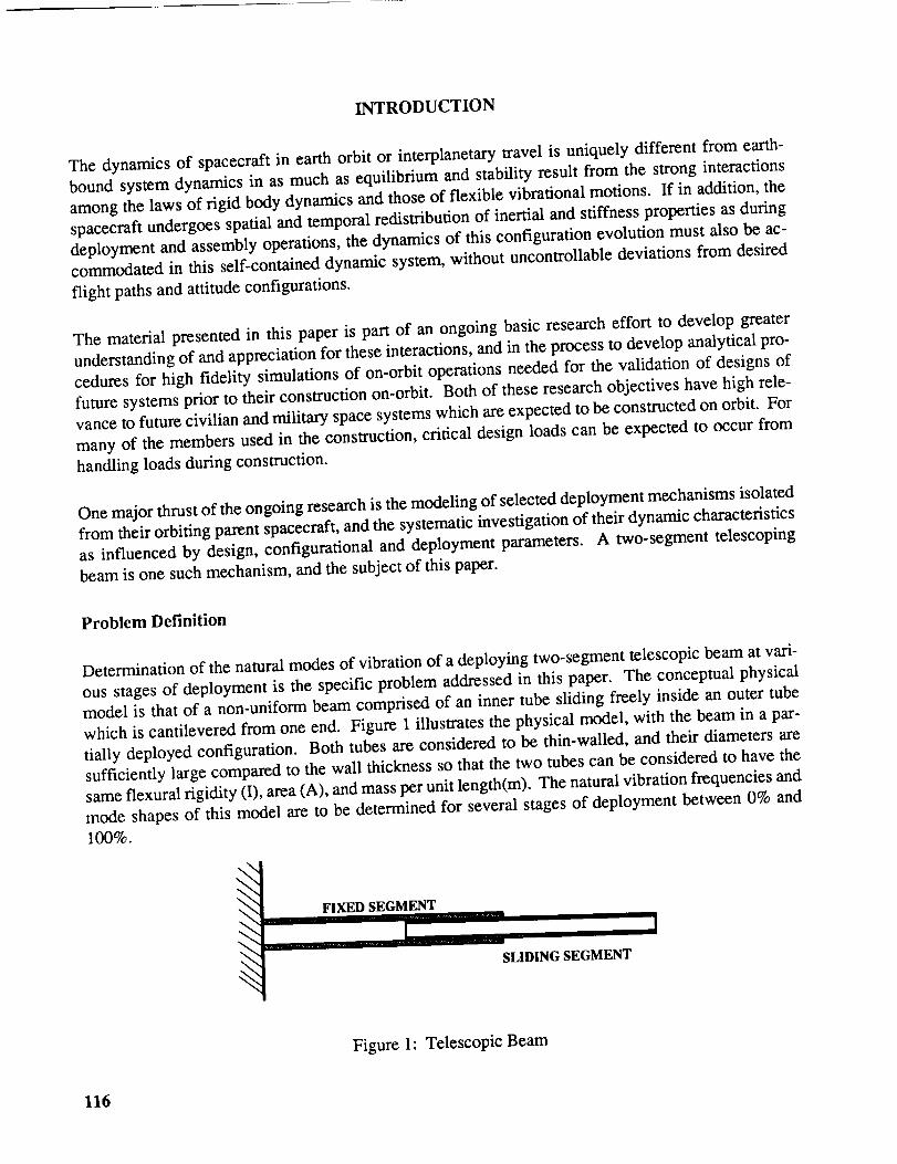
which is cantilevered from one end. Figure 1 illustrates the physical model, with the beam in a par-

tially deployed configuration. Both tubes are considered to be thin-walled, and their diameters are

sufficiently large compared to the wall thickness so that the two tubes can be considered to have the

same flexural rigidity (I), area (A), and mass per unit length(m). The natural vibration frequencies and

mode shapes of this model are to be determined for several stages of deployment between 0% and

100%.

FIXED SEGMENT _1

Figure 1: Telescopic Beam

116

Equationsof Motion

MATHEMATICAL MODELING

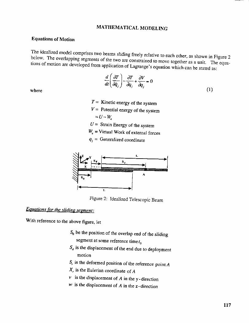
The idealized model comprises two beams sliding freely relative to each other, as shown in Figure 2

below. The overlapping segments of the two are constrained to move together as a unit. The equa-

tions of motion are developed from application of Lagrange's equation which can be stated as:

_" -_+_,=0

where (1)

T = Kinetic energy of the system

V = Potential energy of the system

=U-W

U = Strain Energy of the system

= Virtual Work of external forces

qj = Generalized coordinate

&Z y j_ L I

S0"_1 / A

L

Figure 2: Idealized Telescopic Beam

Equations for the sliding segment:

With reference to the above figure, let

So be the position of the overlap end of the sliding

segment at some reference time t o

S d is the displacement of the end due to deployment

motion

S, is the deformed position of the reference point A

X, is the Eulerian coordinate of A

v is the displacement of A in the y- direction

w is the displacement of A in the z- direction

ll7

Thent

s.=_w#tto

1 x,[-/03VX2 _ 2

whereUo = Deployment velocity

u, = Displacement of A due to elasticity

The velocity vector of A is then given by:

_1 ._ " _ _ __---[Uo +ti, _lv"_+v-_+(v--_+w--_)]'i+_']+¢vk

Now define a displacement u such that

1(¢_+ 030 fi, OW+w°_" ]-- V-_-+

(2)

(3)

(4)

(5)

Then

The kinetic energy of the system can now be determined as

1 L

r=_mJ_._ax1 L

2

The strain energy and virtual work quantities can be expressed as

(6)

(7)

1 LF t'O2v_2 (0_ 2W'_ 2 (8)

wherepy andp_ are external distributed loads.(9)

118

It should be noted that in the above equations, the variable u introduced by definition is not a

state variable like v and w, but is rather a function of the last two and the elastic displacement u e.Hence the generalized coordinates are Ue, v, and w.

Performing the variations indicated in the Lagrange's equations, and noting that, as in Hamilton's

Principle, admissible variations all vanish at the boundaries of the integration domain, thefollowing nonlinear and non-autonomous equations result.

O_ 2Ue

mii - EA---_- = 0

-+

m[w - _- _ti -_-- + _i ._.. + .___. : p,

Equations for the Fixed Segment:

(lO)

(11)

(12)

The above equations are directly applicable to the fixed segments with the modification that thequantity u is defined without the deployment velocity UD, i.e.

1 .&

u = u, -_(v-_+ v_+ w_-+ w_)

Characteristic Equations

(13)

For the purpose of determining the modal characteristics, the above equations of motion are

reduced to a quasi-static form by dropping the deployment velocity related terms and allnonlinear terms to yield

- EA 032u"mii c9x2 = 0

.O_4V

mP + EI-_--g = 0

(14A)

(14B)

_d4w

mCO+ el--_- = O (14C)

119

The equations are completely uncoupled and can be studied independently of one another. The

following treatment is therefore confined to vibrations in the x-z plane, governed by the last of

the three equations above. This is a standard beam equation of the Euler-Bernoulli type. The

homogeneous part defines the modal characteristics of the beam system.

The general solution of the homogeneous equation is given by:

w(x,t) =(a, cosh fix + A2 sinh fix + a 3 cos fix + A, sin fix)sin(tot - q_) (15)

= ¢ (x) sin(a._t - tp)

where

13' = to 2 _// (16)

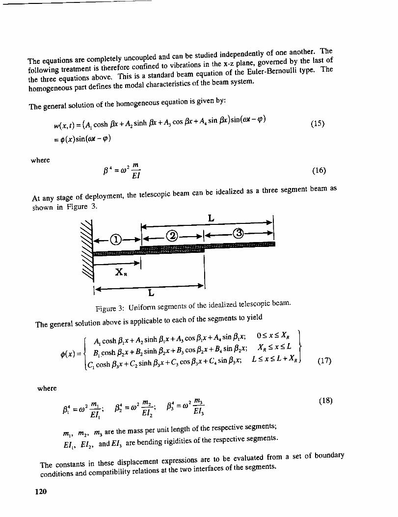
At any stage of deployment, the telescopic beam can be idealized as a three segment beam as

shown in Figure 3.

"': -@

L

Figure 3: Uniform segments of the idealized telescopic beam.

The general solution above is applicable to each of the segments to yield

[ Atcosh/31x+A2sinh/3Lx+A3cos/3tx+A4sin/31x; O<_x<_Xn

_(x) = t Bt cosh/32 x + B2 sinh/32x + B3 cos f12x + B4 sin/32x; X R <_x <_L

[C1 cosh/3sx + C2 sinh/33x + Cs cos/33x + C4 sin/33x; L < x <_L + XR(17)

where

.2 m2 .

___to2 /3;=,o /3;=to2m3el--7'(18)

m_, m2, ms are the mass per unit length of the respective segments;

EI_, EI2, and EI s are bending rigidities of the respective segments.

The constants in these displacement expressions are to be evaluated from a set of boundary

conditions and compatibility relations at the two interfaces of the segments.

120

Theboundaryconditionsaregivenby:

_,(o)=o

a¢(0) =0dr

d%(L+X.)=0

dr2

d303(L+X,,)=0

ddf 3

and the compatibility conditions are given by

(19)

dr dr

ei, d:¢,l(X,,)dr 2 =El2

el_ a_¢(x.)dr3 =El2

¢:(t) = ¢_(L)

a¢:(L) d¢3(L)

dr2

dr3

dr dr

E12 dSq)2(L) d:$3(L )dr2 = EI3 dr2

d3_:(L)=EI3 d3_3 (L)dr3 dr3

(20)

Introducing the appropriate functions into these conditions results in twelve homogeneous

equations. The determinant of the coefficient matrix must vanish for non-trivial solution of theconstants. Hence

=0

(21)

121

where

11° [A]=0 1 0

cosha 1 sinhal cosal sinai 1

B / fllsinhal fllc°shal -fllsinal fllc°sal /

E11 -EI 1cosal -El I sin all[ ]=lEllcosha I sinh al

[.El 1sinhal E1t coshat Ell sinai -EI1 cosal.]

I -c°sh a2 -sinha2 -c°sa2 -sin a2 1

_flEsinha2 -21 cosha2 _sina2 -3"1 c°sa2 |

[C]= __2El2cosha 2 __t2Ei2sinha2 _2EI2cosa 2 _2EIEsina2/

-_3EI2 sinha 2 -_3EI2 cosha 2 -_3EI2 sin a 2 _a3E12 cosa2_l

cosha3 sinha3 cosa3 sina3 1

_ . /sinha3 cosha3 -sinc% c°sa3 /

[D]=/cosha3 sinha3 -cosa3 -sina3|[_sinh a3 cosha3 sina3 -cosa3J

- co sh a4

= [ -22 sinh a4

[El 1-22 2 cosha4

[.-223 sinh a4

_sinha 4 -cosa4 -sina4 1

sin a4 -22 cosa4

-22cosha, 2222-22_ sinh a4 cosa4 22 2 sin a4

_223cosha4 _223sina4 223cosa 4

cosha_ sinha s -cosa s -sina s]

[F] = Lsinha 5 cosha5 sina5 -cosasJ

(22)

(23)

(24)

(25)

(26)

(27)

and_2

a, = #3L; 22=-_

The determinant equation is nondimensionalized by introducing

k =fltL; _R. =

(28)

(29)

122

Then

a 3 = _k; a4 = _ _k; as = Aa _k(l+_.) (30)

SAMPLE RESULTS AND DISCUSSION

A numerical algorithm has been developed for solving the determinant equation for a specified

number of the first consecutive eigenvalues (kn) of the system and the correspondingeigenvectors representing the unknown coefficients of the displacement functions. The modeshapes are also calculated from the eigenvectors.

Table 1 lists the first 10 eigenvalues for a number of deployment stages. The first and last

columns represent data for straight beams at the fully collapsed and at the fully deployed lengths.Figure 4 is a graphical display of the same data.

Mode #

1

2

3

4

5

6

7

8

9

10

IBL for Different De loyment Stages(_)

5 [ i0 I 25 I__ 9-"--'__1.8751 1.7739 1.6959 1.5325 1.3527 1.2115 1.1360 1.11204.6941 4.4846

7.8548 7.5461

10.996 10.400

14.137 10.503

17.279 10.712

20.420 10.812

23.562 10.910

26.704 11.000

29.845 11.100

4.3572

7.3600

9.2000

9.2001

9.7300

9.8100

9.9112

10.010

10.600

4.0142 3.2388

6.4243 5.0683

8.5100 7.2910

8.8400 7.3110

9.0030 7.4015

9.1010 7.5011

9.2004 7.6000

9.6100 8.1545

9.7200 8.2100

2.6482

4.4664

6.2220

7.0904

7.1000

7.9100

8.0100

8.1120

8.2004

100

0.9375

2.ddd2 2.3985 2.3470

4.1495 4.0468 3.9274

5.7000 5.5600 5.4980

6.7390 7.0318 7.0685

6.8010 7.1000 8.6395

7.3003 7.3103 10.210

7.6293 7.8314 11.781

7.7002 8.0000 13.3527.9401 R 1_;t_ la o,_,_

Table 1: Frequency Parameter Variations with Deployment

Two trends are immediately evident from the data:

1. A compaction of the frequencies towards the lower end as deployment proceeds, thus

increasing the modal density in regions of normal dynamic interest, and

2. The appearance of very close, nearly repeated roots from about the third mode upwards,for all the partially deployed configurations

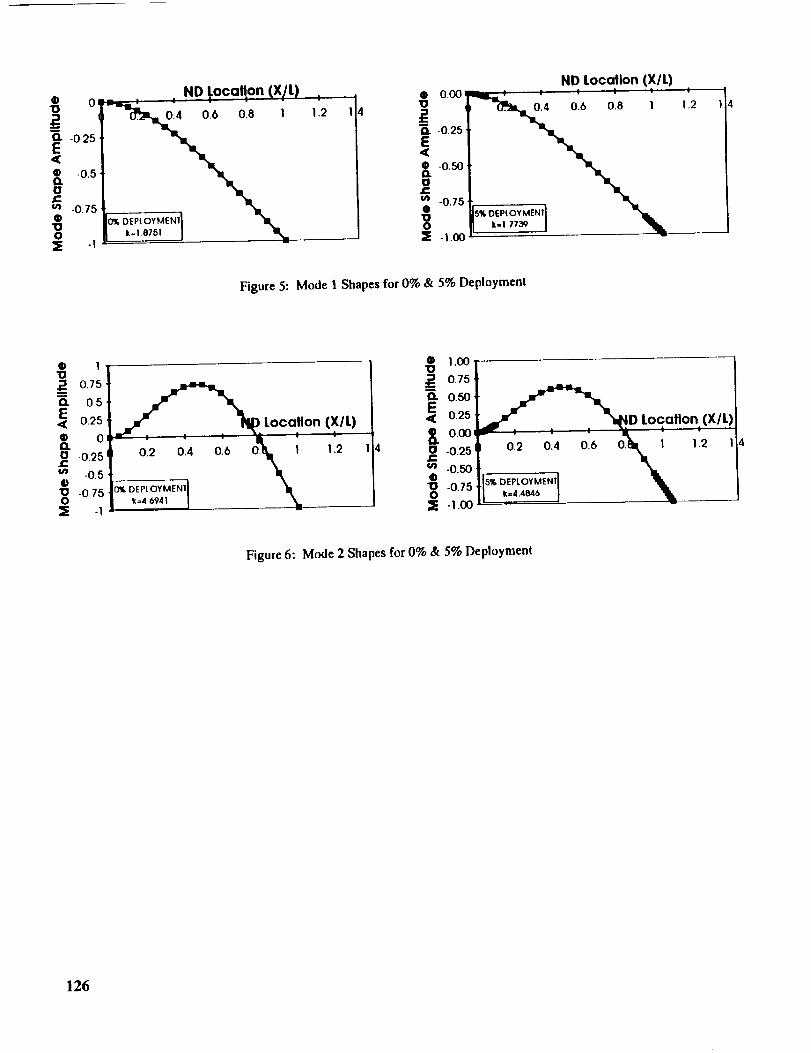
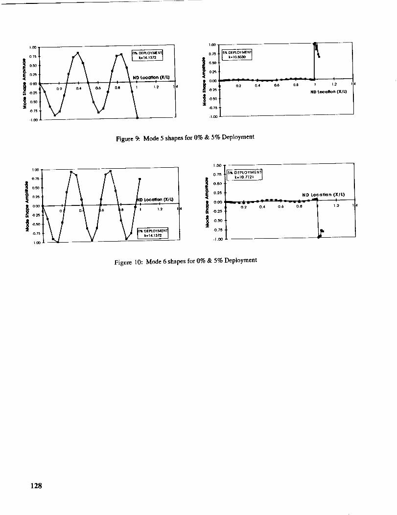
The mode shapes provide clues as to the basis for these trends. Figures 5 through 10 show the

first six mode shapes for the 0% and 5% deployment configurations. The first four mode shapes

are very similar for the two configurations. The fifth and sixth differ markedly between the two

configurations. The partially deployed configuration shows large motions in that portion of the

deploying segment that protrudes from the fixed segment in comparison with the motions of the

fixed segment. These modes can properly be described as "tip whip" modes, in analogy with the

classical "antenna whip "motions of automobile radio antennas. The fixed segment is seen to be

123

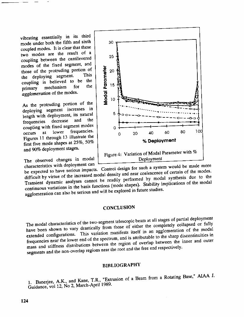
vibrating essentially in its third

mode under both the fifth and sixth

coupled modes. It is clear that thesetwo modes are the result of a

coupling between the cantileveredmodes of the fixed segment, and

those of the protruding portion of

the deploying segment. This

coupling is believed to be the

primary mechanism for the

agglomeration of the modes.

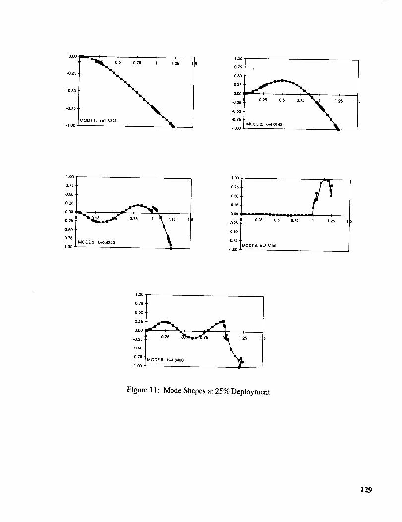
As the protruding portion of the

deploying segment increases in

length with deployment, its natural

frequencies decrease and the

coupling with fixed segment modesoccurs at lower frequencies.

Figures 11 through 13 illustrate thefirst five mode shapes at 25%, 50%

and 90% deployment stages.

The observed changes in modal

characteristics with deployment can

3°I25

•_ 20

5 -o.- !/ ..... "0--

O_ =" I = I • I E I ="_

0 20 40 60 80

% Deployment

Figure 4: Variation of Modal Parameter with %Deployment

be expected to have serious impacts. Control design for such a system would be made more

difficult by virtue of the increased modal density and near coalescence of certain of the modes.

Transient dynamic analyses cannot be readily performed by modal synthesis due to the

continuous variations in the basis functions (mode shapes). Stability implications of the modal

agglomeration can also be serious and will be explored in future studies.

CONCLUSION

The modal characteristics of the two-segment telescopic beam at all stages of partial deployment

have been shown to vary drastically from those of either the completely collapsed or fully

extended configurations. This variation manifests itself in an agglomeration of the modal

frequencies near the lower end of the spectrum, and is attributable to the sharp discontinuities in

mass and stiffness distributions between the region of overlap between the inner and outer

segments and the non-overlap regions near the root and the free end respectively.

BIBLIOGRAPHY

1. Banerjee, A.K., and Kane, T.R., "Extrusion of a Beam from a Rotating Base," AIAA J.

Guidance, vol 12, No 2, March-April 1989.

124

2. Kalaycioglu, S. and Misra, A.K., "Analytical Expressionsfor Vibratory DisplacementsofDeployingAppendages,"AIAA paper88-4250-CP,1988.

3. Modi, V.J., and Ibrahim, A.M., "A General Formulation for Librational Dynamics ofSpacecraft with Deploying Appendages," AA J. Guidance, vol 7, No 5, Sept-Oct 1984.

4. Tsuchiya, K., "Dynamics of a Spacecraft DuringExtension of Flexible Appendages," AIAAJ. Guidance, vol 6, No 2, 1983.

5. Ibrahim, A.E., and Misra, A.K., "Attitude Dynamics of a Satellite During Deployment ofLarge Plate-Type Structures," AIAA J. Guidance, vol 5, No 5, Sep-Oct 1982.

6. Lips, K.W., and Modi, V.J., "Three-Dimensional Response Characteristics for Spacecraftwith Deploying Flexible Appendages," AIAA J. Guidance and Control, vol 4, No 6, Nov-Dec1981.

7. Tabarrok, B., Leech, C.M., and Kim, Y.I., " On the Dynamics of an Axially Moving Beam,"J. Franklin Institute, vol 297, pp 201-220, 1974.

8. Atluri, S.N. and Amos, A.K.,(ed) Large Space Structures: Dynamics and Control, Springer-Verlag, 1988.

ACKNOWLEDGEMENT

This research is sponsored by the Air Force Office of Scientific Research (AFOSR) under Grant

AFOSR-91-0155. The guidance and encouragement of the project director Dr. Spencer Wu aregreatly appreciated.

125

• O:"0

_2D. -0.25E<

@ -0,5nDt-

-0.75®"00=E "!

_ : , ND _oco.on (X/L)

k=,.eTm I ",-

1.2 I i 0.00

(3. -0.25E<@ -0.50

Om-

-0.75®100=E -1.oo

ND toccdlon (X/t)

Figure 5: Mode I Shapes for 0% & 5% Deployment

I _ 1.00

o5i.,,o75 o+O+i..,<E 0.25 Locotlon (X/L) E 0.25 D Locoflon(X/t)

•_ o -- _ , , A. ' .. O.00_r--' ' ' "4 ; " "-.o._o._o.,o+_, , ,._,_ o.+t o.2o.,o.oo.\, ,._,_ -0.7 -0.7 k=4.4846

o :_.,.oo

Figure 6: Mode 2 Shapes for 0% & 5% Deployment

126

1.00.

-_ 0.75

O5O

E 0,25

. 0.000i- -0.25

• -0.50

II-o.z5

-1,00

0% DEPLOYMEN| 1

. _°7._8I

i ___\: ' :o,

Figure 7: Mode 3 Shapes for 0% & 5% Deployment

1.013-

0 75 •

050-

E o25<

a 0._

025

_ .t) 50

IE075

-I.00

_ o_PLoY,.E.4 T

:___/_,o'.' , '""°'77''_:

|00.

0.75 .

0,50.

E o26.

[ 000:

"0.25

-0 15

-I,1_

5% DEPLOYMENT I ]

k.lo_1 /,_ I

04 0._ _ I 12

(x/t)

Figure 8: Mode 4 Shapes for 0% & 5% Deployment

127

l,O0

0 75

i 0,50,

E o2s,

i 000

O, 75

-I.00

_j= JOe. Df PLOYMENTI

' _/: ':" '"i'_'x''

ii!15,°_t°YM,._I k.lo.so3o/o,oo - :---" --- : ..... --: '

0.2 o., 0.6 0.8 ,.2-0.25

NO Location (X/L]

_ -0._

40.75

-1,00

Figure 9:. Mode 5 shapes for 0% & 5% Deployment

|.00.

075 •

I 0.50

"_ 025

i -025-0,50

O. 75 •

-1OO

0.25 I ....

_ k=lO./121 j

0.2

NO Location (X/L]

__..___-_. =_ __.=_,,mi- f0.4 0.6 0.8 1.2

Lz'

Figure 10: Mode 6 shapes for 0% & 5% Deployment

128

°251I

-0.75 IMOD E | : k=1.5325

-I ,00 4.

1.00

0.75

0.50'

0.25 '

0,00

-0.25

-0.50

-0,75

-I .00

_I.MoOE2:k=4.0142 _25

1.00 ¸

0,75 ,

0.50.

0.25

0.00

-0.2,$

-0.50

-0.75

-I .130

_1 "___ I

0.75 I _.25

MO£)E 3:k=6.4243 _

1.00

0.75

0.50

0.25

0,00:

-0.25 1

-0.50

-0.75

-1.00

0.25 0.5 0,75 ! 1,25

_IODE 4:k=8.5100

1,00

0,75

0.50,

0,25

0,00

-0.25

-0,50

-0.75

-I .00 VlODE 5:k=8.8400

Figure 11: Mode Shapes at 25% Deployment

129

0.00

-0.25

-0.50,

-0.75

-I 00

-- : _, I I I 15

MODE I: k:I.3527 _,

1.75

1.00

0.75

0.50

0.25

0.00 q

-0.25 '

-0.50

-0.75

-I .00O : k=

1.00'

0.75

0.50

0,25

0.00

-0.25

-0.50

-0.75

-I,00MODE 3:k=5.0b83

1.00' ._.

0.75 •

0.50'

0.25 ' _ ,_

- _5-0,25

-0,50

-0.75

O k=-I .00

I

1.75

0.25 . .

-0.25

:::I\ / v-I.00 _ MODE 5:_7.311

Figure 12: Mode Shapes at 50% Deployment

130

0.00

-0,25

-0.50

-0.7.5

-1.00

I !

2 2.25

1.00

0.75

0.60.

0.25

0.00

-0.25

-0.50,

-0,75

-I .00

025 05 075 I 125 2 2.25

_IODE 2:k-2.4442

1.00

0.75

0.80

0.25

0.00 :

-025

-0.50

-0.75

-I ,00

25o_oo;__,7_ ; 2,'2°/lODE 3:k_4.1495

1.00

0.76

0.50

0.25

0,00:

-0.25

-0.50

-0.75

-I .00_ODE 4:k=5,7000

i

2 2,25

],C_-

0.75

0.50

0,25

0.00:

-0.25 J

-0.50

-0.75

-1.00

MODE 5:k=6.7390

Figure 13: Mode Shapes at 90% Deployment

131

AEROELASTICITY APPLICATIONS

I:Sq_AII)_N.G P,q;;E _a..';K NOT F,_LI_._

133

/i

/

/'/